nonequilibrium thermodynamics and statistical … · nonequilibrium thermodynamics and statistical...
TRANSCRIPT
NONEQUILIBRIUM THERMODYNAMICS AND STATISTICAL
PHYSICS OF SURFACES
D . BEDEAUX
Department of Physical and Macromolecular Chemistry Gorlixeaus Laboratories. University of Leiden
Leiden. The Netherlands
CONTENTS
I . Introduction ............................................................ A . Historical Remarks .................................................. B . On the Mathematical Description of Interfaces .........................
I1 . Conservation Laws: ...................................................... A . Introduction ........................................................ B . Conservation of Mass ............................................... C . The General Form of Interfacial Balance Equations .................... D . Conservation of Momentum .......................................... E . Conservation of Energy ..............................................
111 . Entropy Balance ........................................................ A . The Second L.aw of Thermodynamics ................................. B . The Entropy .Production .............................................
IV . The Phenomenological Equations ......................................... A . Introduction ........................................................ B . The Curie Symmetry Principle ........................................ C . The Onsager Relations ............................................... D . Symmetric Traceless Tensorial Force-Flux Pairs ........................ E . Vectorial Force-Flux Pairs ........................................... F . Scalar Force-Flux Pairs .............................................. G . The Normal Components of the Velocity Field at the Dividing Surface ... H . The Liquid-Vapor Interface ..........................................
V . Equilibrium Fluctuations of a Liquid-Vapor Interface ....................... A . Introduction ........................................................ B . Fluctuations in the Location of the Dividing Surface .................... C . The Equilibrium Distribution ......................................... D . The Height-Height Correlation Function ............................... E . The Average Density Profile ......................................... F . The Density-Density Correlation Function ............................. G . Spectral Representation of the Density-Density Correlation Function in
47 the Capillary-Wave Model ...........................................
48 48 50 57 57 57 60 61 64 65 65 66 71 71 72 74 75 75 77 80 81 85 85 87 88 91 93 95
97
Advance in Chemical Physics, Volume LXIV Edited by I. Prigogine, Stuart A. Rice
Copyright © 1986 by John Wiley & Sons, Inc.
48 D. BEDEAUX
H. A General Identity for the Density-Density Correlation Function ........ 99 I. The Direct Correlation Function in the Capillary-Wave Model ........... 101
VI. Time-Dependent Fluctuations of a Liquid-Vapor Interface ................... 103 A. Introduction ........................................................ 103 B. Fluctuation-Dissipation Theorems for Excess Random Fluxes at the Inter-
face ................................................................ 105 References.. ............................................................ 107
I. INTRODUCTION
A. Historical Remarks
A consistent phenomenological theory of irreversible processes con- taining both the Onsager symmetry relations and an explicit expression for the entropy production was formulated by Meixner' in 1941 and somewhat later by Prigogine.2 This was the beginning of the field of nonequilibrium thermodynamics, which developed subsequently in many different directions. In 1962 a book on this subject by de Groot and Mazur3 was published, which discussed the developments up to that time; it is still the standard text in this field. The method has also been used to describe transport processes through membranes:
This chapter will discuss the use of this general method in the phenomenological description of irreversible processes that take place at a surface of discontinuity between bulk phases. The equilibrium proper- ties of surfaces of discontinuity were discussed extensively by Gibbs' in the context of his work on the equilibrium thermodynamics of heterogeneous substances. A general method for the application of non- equilibrium thermodynamics to surfaces of discontinuity consistent with the equilibrium theory for surface thermodynamics formulated by Gibbs was given a hundred years later by Bedeaux, Albano, and Mazur.6
One of the dficulties in such an analysis is that the surface of discontinuity not only may move through space but also has a time- dependent curvature. This makes it necessary to use time-dependent orthogonal curvilinear coordinates for the more difficult aspects of the analysis. A shock-wave front, which has no equilibrium analog, may also be described as a moving surface of discontinuity.
The theory gives an explicit expression for the excess production of entropy at the surface of discontinuity. This expression makes it possible to identify the appropriate forces and fluxes. Onsager symmetry relations for the linear constitutive coefficients relating these forces and fluxes are given by the theory. The expression for the fluxes through the surface of discontinuity from one bulk phase to the other lead to the usual boundary
NONEQUILIBRIUM THERMODYNAMICS AND STATISTICAL PHYSICS 49
conditions containing as constitutive coefficients, for example, the slip coefficient and the temperature-jump coefficient. Other fluxes charac- terize the flow along the interface and the flow from the bulk regions into the interfacial region and vice versa. The excess entropy production contains the fluxes through and into the surface of discontinuity in the reference frame in which this surface is at rest. This fact gave rise to considerable discussion among workers in the field of membrane trans- port.7
The tensorial nature of the fluxes and forces contributing to the excess entropy production at the surface of discontinuity differs from the corre- sponding behavior in the bulk regions. The reason for this is that the surface of discontinuity breaks the symmetry; there is still symmetry for translation and rotation along the surface, but not in the direction normal to the surface. As a consequence the force-flux pairs contributing to the excess entropy production at the surface of discontinuity contain 2 X 2 tensors, two-dimensional vectors, and scalars, rather than 3 X 3 tensors, three-dimensional vectors, and scalars as in the bulk regions. The number of force-flux pairs is found to be larger than the number of force-flux pairs in the bulk regions, and as a consequence, the number of indepen- dent constitutive coefficients needed for a complete description of dynamic processes around the surface of discontinuity is much larger than the number of constitutive coefficients needed in the bulk regions. This large number is needed even though, as a consequence of Curie's symmetry principle, fluxes depend only on forces of the same tensorial nature. The resulting large number of different dynamical phenomena in the neigh- borhood of a surface of discontinuity is what makes this such an interest- ing region.
Subsequent work?'' extended the original analysis, which was given for a surface of discontinuity between two immiscible one-component fluid phases, to multicomponent systems with mass transport through the surface of discontinuity' and including electromagnetic effects? The theory was further extended by Zielinska and Bedeauxl' to describe spontaneous fluctuations around equilibrium, in which context fluctuation-dissipation theorems were given.
In Sections, 11, 111, and IV of this chapter we shall discuss, the conservation laws, the entropy balance, and the phenomenological equa- tions for a surface of discontinuity between multicomponent phases in which chemical reactions and mass transport through and into the surface are possible.
In Section V we analyze the equilibrium (equal-time) correlations at a liquid-vapor interface. Expanding the excess entropy of the system to second order in the fluctuations, we find, in addition to the contributions
50 D. BEDEAUX
due to the displacement of the interface and usually given in the capillary- wave theory,12 contributions due to for example, interfacial temperature and velocity fluctuations. These expressions are given in the general case of a nonplanar equilibrium shape of the interface. Some recent work by Bedeaux and Weeks13 on the behavior of the densityaensity correlation function and the direct correlation function in the neighborhood of the interface is discussed. For the density-density correlation function, their expressions are generalized to the case of finite bulk compressibilities.
In Section VI the description is extended by the inclusion of random fluxes. Fluctuation-dissipation theorems for these random fluxes are given.
The general method of nonequilibrium thermodynamics is, as we shall discuss in more detail, inherently limited to the description of time- dependent phenomena over distances large compared with the bulk correlation length. We shall therefore not discuss the behavior near and in the surface of discontinuity on a molecular level. The reader is instead referred to the extensive literature on this subject. l4
B. On the Mathematical Description of Interfaces
We consider here dynamical processes of a system in which two phases coexist. The phases are separated by a moving surface of discontinuity, or interface as we shall often call it, with a time-dependent curvature. The term “surface of discontinuity” does not imply that the discontinuity is sharp, nor that it distinguishes any surface with mathematical pre~is ion.~ It is taken to denote the nonhomogeneous film that separates the two bulk phases. The width of this film is on the order of the bulk correlation length.
In the mathematical description of the dynamical properties of the system, we want to choose a method such that details of the description on length scales smaller than the bulk correlation length do not play a role. In the bulk phases, this implies that one replaces, for example, the molecular density by a continuous field that is obtained after averaging over cells with a diameter of the order of the bulk correlation length. Such a procedure gives an adequate description of the behavior of a bulk phase on a distance scale large compared with the bulk correlation length if the variation of the fields over a bulk correlation length is small. The surface of discontinuity is, in this context, a two-dimensional layer of cells in which the variables change rapidly in one direction over a distance of the order of a bulk correlation length from the value in one phase to the value in the other phase, but change slowly in the other two directions. One now chooses a time-dependent dividing surface in this two- dimensional layer of cells such that the radii of curvature are large compared with the bulk correlation length. Surfaces of discontinuity for
NONEQUILIBRIUM THERMODYNAMICS AND STATISTICAL PHYSICS 51
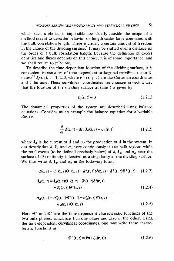
which such a choice is impossible are clearly outside the scope of a method meant to describe behavior on length scales large compared with the bulk correlation length, There is clearly a certain amount of freedom in the choice of the dividing surface.' It may be shifted over a distance on the order of a bulk correlation length. Because the definition of excess densities and fluxes depends on this choice, it is of some importance, and we shall return to it below.
To describe the time-dependent location of the dividing surface, it is convenient to use a set of time-dependent orthogonal curvilinear coordi- n a t e ~ : ~ ~ &(r, t ) , i = I, 2 ,3 , where r = (x, y, z ) are the Cartesian coordinates and t the time. These curvilinear coordinates are choosen in such a way that the location of the dividing surface at time t is given by
The dynamical properties of the system are described using balance equations. Consider as an example the balance equation for a variable d(r, t ) :
a at - d (I, t ) -k div Jd (r, t ) = (r, t ) (1.2.2)
where J d is the current of d and a d the production of d in the system. In our description d, J d and a d vary continuously in the bulk regions while the total excess (to be defined precisely below) of d, J d , and a d near the surface of discontinuity is located as a singularity at the dividing surface. We thus write d, J d , and a d in the following form:
d(r, t ) = &(r, t)W(r, t ) + d"(r, t)as(r, t ) + d+(r, t)O'(r, t ) (1.2.3)
&(I, t ) = &(I, t)@-(r, t ) + Ji(r, t)aS(r, t )
+ &(r, t)@+(r, t ) (1.2.4)
(1.2.5)
Here 0- and 0' are the time-dependent characteristic functions of the two bulk phases, which are 1 in one phase and zero in the other. Using the time-dependent curvilinear coordinates, one may write these charac- teristic functions as
W(r, t ) = 0(*,$l(r7 t ) ) (1.2.6)
52 D. BEDEAUX
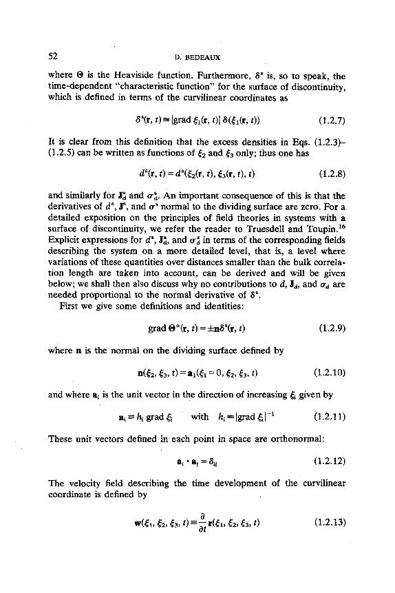
where 0 is the Heaviside function. Furthermore, 8" is, so to speak, the time-dependent "characteristic function" for the surface of discontinuity, which is defined in terms of the curvilinear coordinates as
It is clear from this definition that the excess densities in Eqs. (1.2.3)- (1.2.5) can be written as functions of e2 and t3 only; thus one has
and similarly for J: and u;. An important consequence of this is that the derivatives of d", F, and us normal to the dividing surface are zero. For a detailed exposition on the principles of field theories in systems with a surface of discontinuity, we refer the reader to Truesdell and Toupin. l6 Explicit expressions for d", J:, and CT: in terms of the corresponding fields describing the system on a more detailed level, that is, a level where variations of these quantities over distances smaller than the bulk correla- tion length are taken into account, can be derived and will be given below; we shall then also discuss why no contributions to d, Jd, and ad are needed proportional to the normal derivative of 8'.
First we give some definitions and identities:
grad O*(r, t ) = fnb"(r, t ) (1.2.9)
where n is the normal on the dividing surface defined by
and where ai is the unit vector in the direction of increasing ti given by
ai = hi grad ei with hi = lgrad tit-' (1.2.1 1)
These unit vectors defined in each point in space are orthonormal:
a. 1 a. I = 8.. 11 (1.2.12)
The velocity field describing the time development of the curvilinear coordinate is defined by
NONEQUILIBRIUM THERMODYNAMICS AND STATISTICAL PHYSICS 53
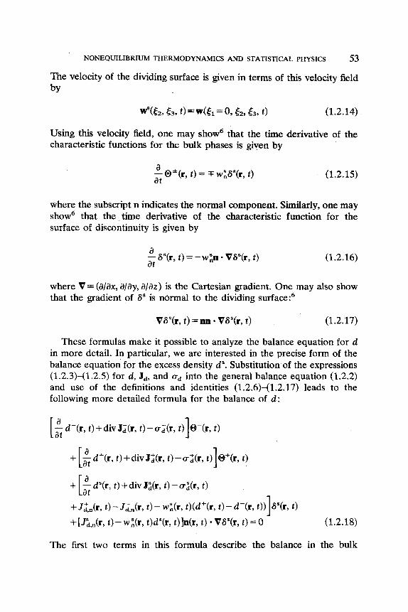
The velocity of the dividing surface is given in terms of this velocity field by
Using this velocity field, one may show6 that the time derivative of the characteristic functions for the bulk phases is given by
- a @*(r, t ) = T w",'(r, t ) at
(1.2.15)
where the subscript n indicates the normal component. Similarly, one may show6 that the time derivative of the characteristic function for the surface of discontinuity is given by
a - iY(r, t ) = -w:n * VSs(r, t ) at
(1.2.16)
where V = (a/&, a/ay, a/az) is the Cartesian gradient. One may also show that the gradient of 6" is normal to the dividing surface?
VS%, t ) = nn Vs'G, t ) (1.2.17)
These formulas make it possible to analyze the balance equation for d in more detail. In particular, we are interested in the precise form of the balance equation for the excess density d". Substitution of the expressions (1.2.3)-(1.2.5) for d, Jd, and a, into the general balance equation (1.2.2) and use of the definitions and identities (1.2.6)-(1.2.17) leads to the following more detailed formula for the balance of d :
The first two terms in this formula describe the balance in the bulk
54
phases :
D. BEDEAUX
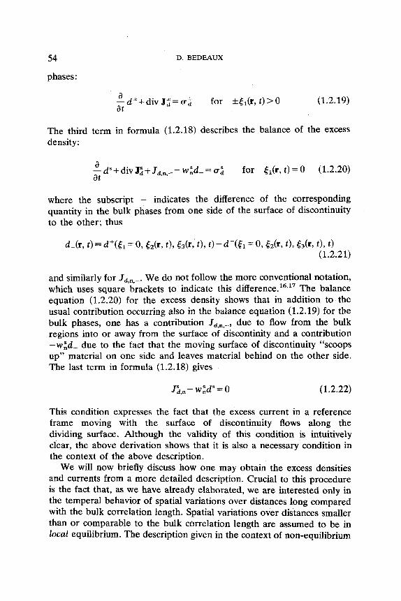
(1.2.19) a at - d* + div J; = CT; for *C1(r, t ) > 0
The third term in formula (1.2.18) describes the balance of the excess density :
a - -d“+divJ~+J, , , , - . -w:d-=u~ for &(r, t ) = O (1.2.20) at
where the subscript - indicates the difference of the corresponding quantity in the bulk phases from one side of the surface of discontinuity to the other; thus
and similarly for Jd,,,-. We do not follow the more conventional notation, which uses square brackets to indicate this diff e r e n ~ e . ~ ~ ” ~ The balance equation (1.2.20) for the excess density shows that in addition to the usual contribution occurring also in the balance equation (1.2.19) for the bulk phases, one has a contribution Jda,-, due to flow from the bulk regions into or away from the surface of discontinity and a contribution -w:d- due to the fact that the moving surface of discontinuity “scoops up” material on one side and leaves material behind on the other side. The last term in formula (1.2.18) gives
J;., - ,Eds = 0 (1.2.22)
This condition expresses the fact that the excess current in a reference frame moving with the surface of discontinuity flows along the dividing surface. Although the validity of this condition is intuitively clear, the above derivation shows that it is also a necessary condition in the context of the above description.
We will now briefly discuss how one may obtain the excess densities and currents from a more detailed description. Crucial to this procedure is the fact that, as we have already elaborated, we are interested only in the tempera1 behavior of spatial variations over distances long compared with the bulk correlation length. Spatial variations over distances smaller than or comparable to the bulk cbrrelation length are assumed to be in local equilibrium. The description given in the context of non-equilibrium
NONEQUILIBRIUM THERMODYNAMICS AND STATISTICAL PHYSICS 55
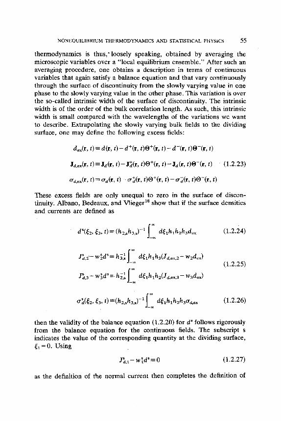
thermodynamics is8 thus,. loosely speaking, obtained by averaging the microscopic variables over a “local equilibrium ensemble.” After such an averaging procedure, one obtains a description in terms of continuous variables that again satisfy a balance equation and that vary continuously through the surface: of discontinuity from the slowly varying value in one phase to the slowly varying value in the other phase. This variation is over the so-called intrinsic width of the surface of discontinuity. The intrinsic width is of the order of the bulk correlation length. As such, this intrinsic width is small compared with the wavelengths of the variations we want to describe. Extrapolating the slowly varying bulk fields to the dividing surface, one may define the following excess fields:
dex(r, t ) = d (r, t ) - d+(r, t)@+(r, t ) - d-(r, t)@-(r, t )
These excess fields are only unequal to zero in the surface of discon- tinuity. Albano, Bedeaux, and Vlieger18 show that if the surface densities and currents are defined as
then the validity of the balance equation (1.2.20) for d“ follows rigorously from the balance equation for the continuous fields. The subscript s indicates the value of the corresponding quantity at the dividing surface,
= 0. Using
J i , l - w;dsG 0 (1.2.27)
as the definition of the normal current then completes the definition of
56 D. BEDEAUX
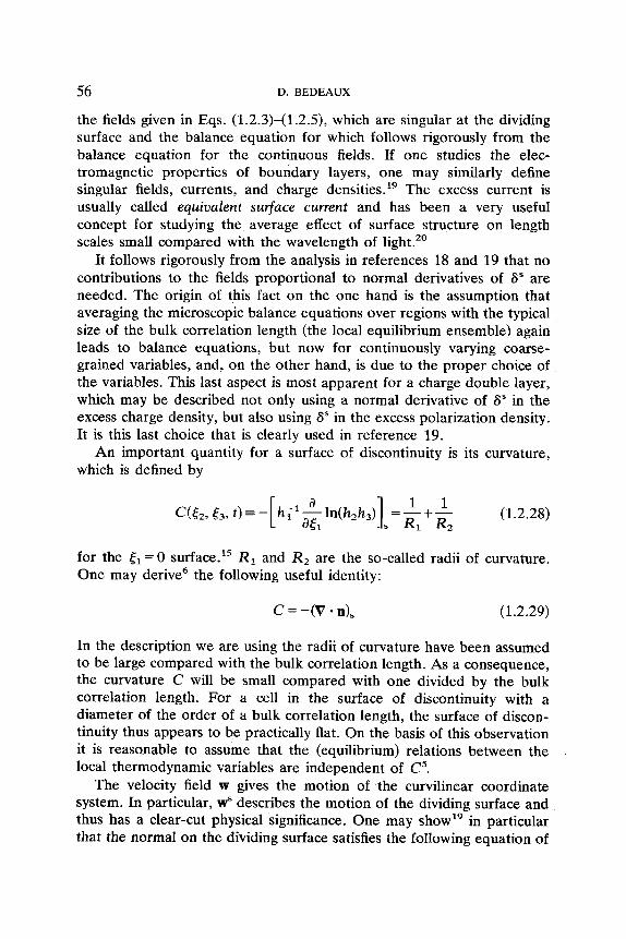
the fields given in Eqs. (1.2.3)-(1.2.5), which are singular at the dividing surface and the balance equation for which follows rigorously from the balance equation for the continuous fields. If one studies the elec- tromagnetic properties of boundary layers, one may similarly define singular fields, currents, and charge densities.lg The excess current is usually called equivalent surface current and has been a very useful concept for studying the average effect of surface structure on length scales small compared with the wavelength of light.20
It follows rigorously from the analysis in references 18 and 19 that no contributions to the fields proportional to normal derivatives of 6" are needed. The origin of this fact on the one hand is the assumption that averaging the microscopic balance equations over regions with the typical size of the bulk correlation length (the local equilibrium ensemble) again leads to balance equations, but now for continuously varying coarse- grained variables, and, on the other hand, is due to the proper choice of the variables. This last aspect is most apparent for a charge double layer, which may be described not only using a normal derivative of 6" in the excess charge density, but also using F s in the excess polarization density. It is this last choice that is clearly used in reference 19.
An important quantity for a surface of discontinuity is its curvature, which is defined by
for the t1 = 0 surface.15 R, and R2 are the so-called radii of curvature. One may derive6 the following useful identity:
c = -(V * n), (1.2.29)
In the description we are using the radii of curvature have been assumed to be large compared with the bulk correlation length. As a consequence, the curvature C will be small compared with one divided by the bulk correlation length. For a cell in the surface of discontinuity with a diameter of the order of a bulk correlation length, the surface of discon- tinuity thus appears to be practically flat. On the basis of this observation it is reasonable to assume that the (equilibrium) relations between the local thermodynamic variables are independent of C5.
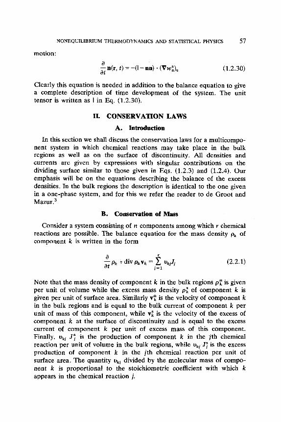
The velocity field w gives the motion of the curvilinear coordinate system. In particular, ws describes the motion of the dividing surface and thus has a clear-cut physical significance. One may showlg in particular that the normal on the dividing surface satisfies the following equation of
NONEQUILIHRIUM THERMODYNAMICS AND STATISTICAL PHYSICS 57
motion: a at - n(r, t ) = -(I - nn) - (Vw:), (1.2.30)
Clearly this equation is needed in addition to the balance equation to give a complete description of time development of the system. The unit tensor is written as I in Eq. (1.2.30).
11. CONSERVATION LAWS
A. Introduction
In this section we shall discuss the conservation laws for a multicompo- nent system in which chemical reactions may take place in the bulk regions as well as on the surface of discontinuity. All densities and currents are given by expressions with singular contributions on the dividing surface similar to those given in Eqs. (1.2.3) and (1.2.4). Our emphasis will be on the equations describing the balance of the excess densities. In the bulk regions the description is identical to the one given in a one-phase system, and for this we refer the reader to de Groot and M a ~ u r . ~
B. Conservation of Mass
Consider a system consisting of n components among which r chemical reactions are possible. The balance equation for the mass density & of component k is written in the form
(2.2.1)
Note that the mass density of component k in the bulk regions p$ is given per unit of volume while the excess mass density pe of component k is given per unit of surface area. Similarly vg is the velocity of component k in the bulk regions and is equal to the bulk current of component k per unit of mass of this component, while vi is the velocity of the excess of component k at the surface of discontinuity and is equal to the excess current of component k per unit of excess mass of this component. Finally, ukl Jf is the production of component k in the jth chemical reaction per unit of volume in the bulk regions, while u k j 7 is the excess production of component k in the jth chemical reaction per unit of surface area. The quantity ukj divided by the molecular mass of compo- nent k is proportional to the stoichiometric coeficient with which k appears in the chemical reaction j.
58 D. BEDEAUX
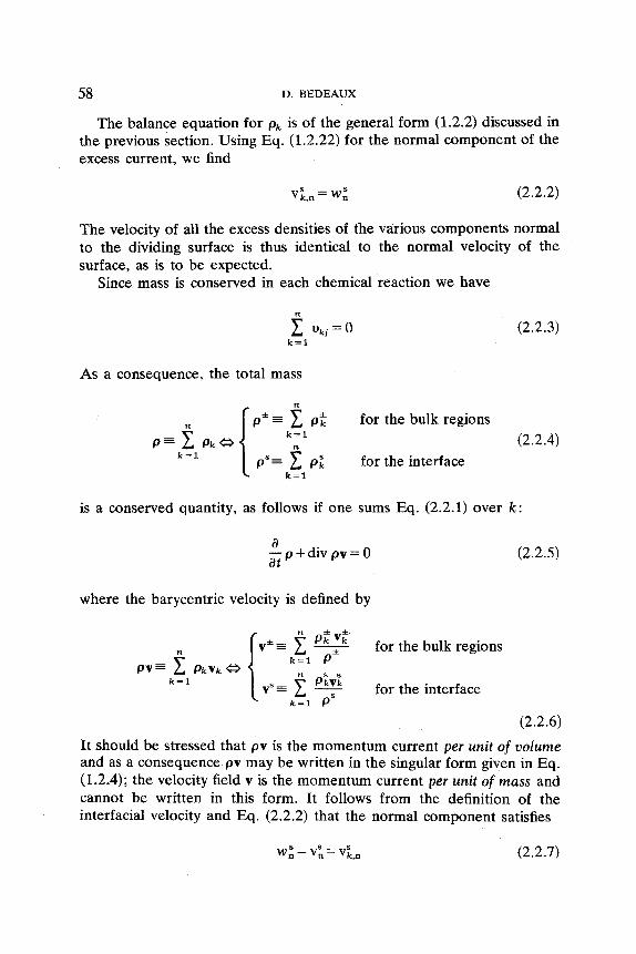
The balance equation for p k is of the general form (1.2.2) discussed in the previous section. Using Eq. (1.2.22) for the normal component of the excess current, we find
v;,n = w; (2.2.2)
The velocity of all the excess densities of the various components normal to the dividing surface is thus identical to the normal velocity of the surface, as is to be expected.
Since mass is conserved in each chemical reaction we have
n
v k j = o k = l
(2.2.3)
As a consequence, the total mass
pc for the bulk regions (2.2.4)
ps= p; for the interface k = l
k = l
is a conserved quantity, as follows if one sums Eq. (2.2.1) over k:
a - p +div pv = 0 at
(2.2.5)
where the barycentric velocity is defined by
p;v;
PSkG
v*= 7 for the bulk regions k = l p
vs= c - for the interface k = l p
k = l
(2.2.6)
It should be stressed that pv is the momentum current per unit of volume and as a consequence pv may be written in the singular form given in Eq. (1.2.4); the velocity field v is the momentum current per unit of mass and cannot be written in this form. It follows from the definition of the interfacial velocity and Eq. (2.2.2) that the normal component satisfies
w ; = vs, = v;,, (2.2.7)
NONEQUILIBRIUhl THERMODYNAMICS AND STATISTICAL PHYSICS 59
Clearly, the dividing surface moves along with the barycentric velocity of the excess mass in the normal direction. We now use the freedom in the choice of curvilinear coordinates to choose them such that this is also the case in the direction parallel to the dividing surface, so that
The advantage of this choice is that the motion of the dividing surface then has a direct physical meaning.
Using the general equation (1.2.20) and Eq. (2.2.7), the balance equation for the excess mass of component k becomes
(2.2.9)
Similarly, one finds for the total excess mass
a - ps + div p%"+ [ p(v,- v31- = 0 at
(2.2.10)
The balance equation for the excess mass of component k can be written in an alternative form if we define the barycentric time derivative for the dividing surface,
d s a --_ = +v".grad dt at
(2.2.1 1)
the bulk and interfacial diffusion flows,
Jc = p:(v: - v*) and J; = pF;(vi - v") (2.2.12)
and the bulk and interfacial mass fractions,
(2.2.13)
Substitution of these definitions into Eq. (2.2.9) and use of Eq. (2.2.10) then gives
60 D. BEDEAUX
It follows from Eq. (2.2.7) that the interfacial diffusion current is along the dividing surface:
n.J;=O (2.2.15)
Furthermore, it follows from Eq. (2.2.6) that
2 J:=O and f: J;=O (2.2.16) k = l k = l
which implies that only n - 1 diffusion currents are independent.
C. The General Form of Interfacial Balance Equations
In the previous section we discussed how the general balance equation (1.2.2) for a quantity d,
(2.3.1) a - d +div Jd =ad at
leads to the following balance equation [cf. Eqs. (1.2.20) and (2.2.7)] for the excess of d :
a -dd”+divJ~+n. [Jd-v”d]-=ai (2.3 -2) a t
Furthermore, one finds the following equation [cf. Eqs. (1.2.22) and (2.2.7)] for the normal component of the excess current:
n [Ji-v”d”l=O (2.3.3)
It is now convenient to define the density of the quantity d per unit of mass by
u* = d*/p*
us= dS/pS for the interface
for the bulk regions (2.3.4) d = p u e
Furthermore, it is convenient to write the current as
Jf = p*u*v* +J*
pd = psusvs + %,
for the bulk region
for the interface (2.3.5) = pQv+ J, e
NONEQUIL~BRIUM THERMODYNAMICS AND STATISTICAL PHYSICS 61
where pav = dv is the convective contribution to the current. Substituting these definitions in Eq. (2.3.2) and using the balance equation (2.2.10) for the excess mass then gives
(2.3.6) d" dt
p s - as + V - J: + n * [ (v - P)p (a - as) + J, 1- = u:
while Eq. (2.3.3) gives
n.J i=O (2.3.7)
These alternative equations, which we shall use often in our further analysis, are, of course, equivalent to the original ones. The results we shall find may also be found using Eqs. (2.3.2) and (2.3.3). In particular, one finds the same results even when the dividing surface can be chosen such that ps = 0. We shall come back to this point below.
D. Conservation of Momentum
The equation of motion of the system
(2.4.1)
where
pvv = p-v-v-0- + p"v"v"8" + p+v+v+o+ (2.4.2)
is the convective contribution to the momentum flow, P is the pressure tensor that gives the rest of the momentum flow, and F, is an external force field acting on component k. The pressure tensor can be written as the sum of the hydrostatic pressures p- and p+ in the bulk regions, minus the surface tension y at the dividing surface and the viscous pressure tensor II both in the bulk regions and on the dividing surface in the following way:
P = p-IO-+p+Io+-y(l-nn)s"+n (2.4.3)
We assume that the system possesses no intrinsic internal angular momentum, so that the pressure tensor and, as a consequence, the viscous contribution are symmetric both in the bulk regions3 and at the inter- face.'l Equation (2.3.7) for the normal component of an interfacial
62 D. BEDEAUX
current gives in this case
where we have used the symmetry. The excess pressure tensor and its viscous part are thus symmetric 2 x 2 tensors. The assumption that scalar hydrostatic pressures and a scalar surface tension can be used limits the discussion to inelastic media. It is easy to extend most formulas to the general case. If a fluid flows along a solid wall it is usually sufficient to take the appropriate fluxes in the wall to be equal to zero in the analysis below.
The forces will be assumed to be conservative and can be written in terms of time-independent potentials:
Fk = -grad $k (2.4.5)
Because of these forces the momentum is not conserved locally, so the equation of motion is a balance equation with xE=lpkFk as source of momentum. Usually the system is contained in a finite box and the total momentum is conserved by interaction with the walls.
Using Eq. (2.3.6) for the momentum density, one finds as the equation of motion for the dividing surface
(2.4.6)
The subscript s indicates, as usual, the value of a field at the dividing surface, obtained by putting el = 0. The limiting value of the field may be different coming from the plus or the minus phase as, for example, for the hydrostatic pressures pf and p;, but may also be the same, as, for example, the forces Fts = FSs = Fk,". Furthermore, it should be stressed that after taking the gradient or divergence of a quantity that is defined oiily on the dividing surface, one should also take the result for ,$*=O. Thus it would, for example, be better to write (VY)~ than Vy; however, for ease of notation we will not usually do this.
Using the fact that the gradient of a quantity defined on the dividing surface (i.e., independent of El) is parallel to this surface, one may write [cf. also Eq. (1.2.29)J
V - y(l -m) = V-y - yn div n = V y + cyn (2.4.7)

NONEQUILIBRIUM THERMODYNAMICS AND STATISTICAL PHYSICS 63
In equilibrium, when v" = 0, IT = 0, and Pi = p*l, Eq. (2.4.6) gives as the balance of the normal components of the forces
n
-C:y + p - = - c y + p z - p l = 2 &Fk,s - n (2.4.8) k = l
This is a direct generalization of Laplace's equation for the hydrostatic pressure difference p z - p ; in terms of the surface tension and the ~urvature. '~ Contraction of Eq. (2.4.6) with the normal gives the generali- zation of Laplace's equation to the dynamic case. In equilibrium Eq. (2.4.6) gives as the balance of the forces along the dividing surface
(2.4.9)
In the general case the normal part of Eq. (2.4.6) describes the motion of the interface through space, while the parallel part describes the flow of mass along the interface.
Using Eq. (2.4.6), one may derive an equation for the rate of change of the kinetic energy of the excess mass:
- n [ (v- v")p(v- vs) + PI- v'
(2.4.10) k = l
The potential energ,y of the excess mass is defined by n
Ps$"E 1 P;$k,k,s (2.4.11)
Using Eq. (2.2.14)' one finds for the rate of change of this potential energy
k = l
(2.4.12) k = l j=l k=l
64 D. BEDEAUX
We shall assume that the potential energy is conserved in a chemical reaction:
n
(2.4.13) k = 1
This is true, for example, in a gravitational field and for charged particles in an electric field. In this case Eq. (2.4.12) reduces to
(2.4.14)
Equations (2.4.10) and (2.4.13) make clear that neither the kinetic energy nor the potential energy, nor, for that matter, their sum, is con- served.
E. Conservation of Energy
According to the principle of conservation of energy, one has” for the total specific energy e
a - pe +div(pev+ J,) = 0 at
(2.5.1)
The total energy density is the sum of the kinetic energy, the potential energy, and the internal energy u :
e* = $(v*I2+ $*+ u*
es= ~lv”I’+ +”+ us
for the bulk regions
for the interface (2.5.2)
Similarly, the energy current may be written as the sum of a mechanical work term, a potential-energy flux due to diffusion, and a heat flow 3,:
(2.5.3)
Equations (2.5.2) and (2.5.3) may be considered as definitions of the internal energy and the heat flow.
* In de Groot and Mazur3 J, contains also the convective contribution.
NONEQUILIBRIUM THERMODYNAMICS AND STATISTICAL PHYSICS 65
The balance equation for the excess energy density is given by [cf. Eq. (2.3.6)1,
(2.5.4) d" dt
p " -- es + V . aS, + n * [ (v - v") p (e - e ") + Je 1- = 0
The excess energy flow is along the dividing surface [cf. Eq. (2.3.7)]:
n.J,s=O (2.5.5)
Using the balance: equations (2.4.10) and (2.4.13) for the kinetic- and potential-energy densities as well as the balance equation (2.5.4) for the total energy, one finds as the balance equation for the excess internal energy
-n - ((v -v")p[ u - us -$\v -v"l"I + Jq + [ (v - V)p (v - v") + PI - (v - V)}- (2.5.6)
It follows from Eqs. (2.2.15), (2.4.4), and (2.5.3) that the excess heat flow is also along the dividing surface:
n*Jt=O (2.5.7)
The internal energy of the system is not conserved, because of conversion of kinetic and potential energy into internal energy. The balance equation (2.5.6) for the excess internal energy gives the first law of ther- modynamics for the interface.
III. ENTROPY BALANCE
A. The Second Law of Thermodynamics
The balance equation for the entropy density is given by
a -pps+div(psv+J)=a (3.1.1) at
where s is the entropy density per unit of mass, J is the entropy current,*
case clearly be confusing. * The subscript s used in de Groot and Mazur3 has been dropped because it would in this
66 D. BEDEAUX
and u is the entropy source. All fields have their usual form (1.2.3)- (1.2.5) containing the excess as a singular contribution at the dividing surface. In the bulk regions, Eq. (3.1.1) gives the usual balance equation for the entropy densities s+ and s-:
(3.1.2)
One may now conclude3 from the second law of thermodynamics that
V*>O (3.1.3)
For the interface, one finds the following balance equation [cf. Eq. (2.3.6)]:
(3.1.4) d" dt
ps - s" = -V - P - n - [ (v - P)p (s - ss) + 31- + us
From the second law of thermodyanics, it now follows that
w S 2 O (3.1.5)
As is to be expected, not only is entropy produced in the bulk regions, but there is also an excess of this production in the interfacial region, which according to the second law is also positive.
B. The Entropy Production
From thermodynamics we know that the entropy for a system in equilibrium is a well-defined function of the various parameters necessary to define the macroscopic state of the system. As discussed already by Gibbs,' this is also the case for a system with two phases separated by a surface of discontinuity. For the system under consideration, we use as parameters the internal energy, the specific volume u* = l /p* or specific surface area us= U p " , and the mass fractions. We may then write
Three different functions are needed to give the entropies for the two bulk phases and for the interface. At equilibrium the total differential of the entropy is given by the Gibbs relation. In the bulk'regions, this
NONEQUILIBRIUM THERMODYNAMICS AND STATISTICAL PHYSICS 67
relation is
n
'P dS'=du*+p* dv'- C p' d? (3.2.2)
where T' is the temperature and p t is the chemical potential of component k in the bulk. For the interface, it is given by5
k = l
n
T S d s S = d u S - y d v S - C FEdcf; (3.2.3)
where T" is the interfacial temperature and p i is the interfacial chemical potential of component k. The Gibbs relation for the interface is in fact similar to the one far the bulk regions if one interprets the surface tension as the negative of the surface pressure, ps=-y.
Though the total system we are describing is not in equilibrium, we assume that the system is in so-called local equilibrium. More particu: larly, we assume that after averaging the microscopic variables over cells with a diameter of the order of the bulk correlation length, one obtains a description in which the local entropy is given, as at equilibrium, by,the functions (3.2.1) in terms of the local values of the internal energy, the specific volume or surface area, and the mass fractions. It is clear that the hypothesis of local equilibrium limits the description to situations where the change of the bulk variables is small over distances of the order of the bulk correlation length in all directions and the change of the excess variables on the dividing surface is small over these distances along the surface. Furthermore, the radii of curvature of the dividing surface must be large compared with the bulk correlation length. This also makes the assumption that s" is not dependent on the curvature a reasonable one. The local-equilibrium hypothesis implies that the Gibbs relation remains valid in the frame moving with the center of mass. We thus have
k = l
in the bulk phases and
(3.2.5)
for the interface. As explained in detail by de Groot and Mazur? one may now find
68 D. BEDEAUX
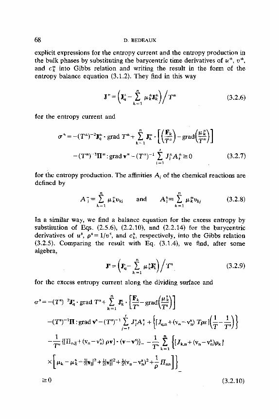
explicit expressions for the entropy current and the entropy production in the bulk phases by substituting the barycentric time derivatives of u*, u*, and c z into Gibbs relation and writing the result in the form of the entropy balance equation (3.1.2). They find in this way
(3.2.6)
for the entropy current and
f
~*=-(T*)-~J$-grad Tf+ J z - [($)-grad($)] k - l
r
-(T*)-lII*:gradv*-(T*)-l 1 JfAfrO (3.2.7) j = l
for the entropy production. The affinities Aj of the chemical reactions are defined by
n n
A;= 1 p* kUkj and c /L+ k vkj (3.2.8) k = l k = l
In a similar way, we find a balance equation for the excess entropy by substitution of Eqs. (2.5.6), (2.2.10), and (2.2.14) for the barycentric derivatives of us7 ps= l /us7 and c i , respectively, into the Gibbs relation (3.2.5). Comparing the result with Eq. (3.1.4), we find, after some algebra,
(3.2.9)
for the excess entropy current along the dividing surface and
-(T")-'II :gradp-(T")-l JsAs t([J,,i(v,-v%) Tpsl($-$)} j = 1
(3.2.10)
NONEQUILIBXUUM THERMODYNAMICS AND STATISTICAL PHYSICS 69
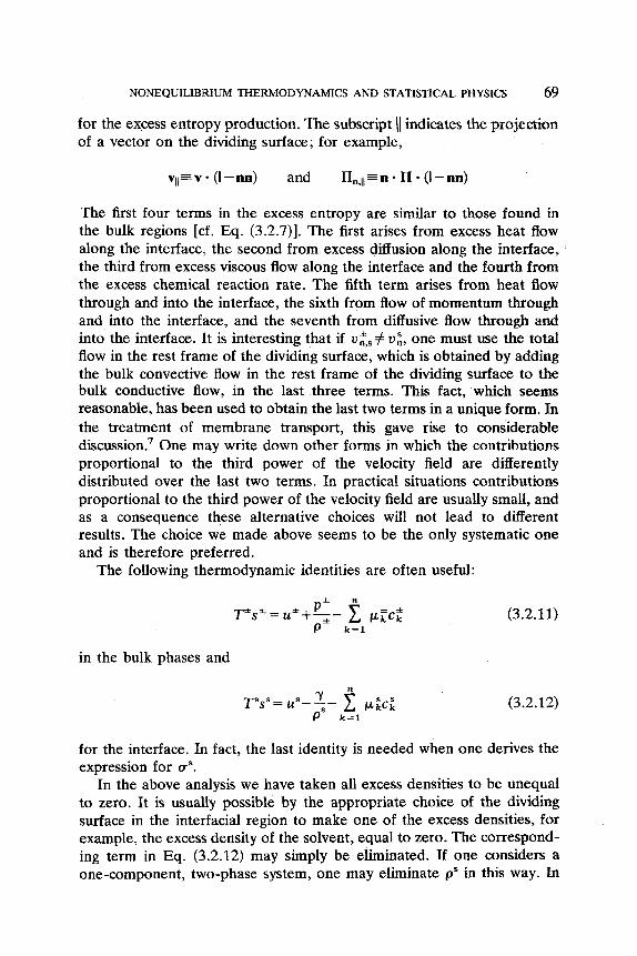
for the excess entropy production. The subscript I\ indicates the projection of a vector on the dividing surface; for example,
VII v - (I - M) and 11,,1, = n ll- (I - M)
The first four terms in the excess entropy are similar to those found in the bulk regions [cf. Eq. (3.2.7)]. The first arises from excess heat Row along the interface, the second from excess diffusion along the interface, the third from excess viscous flow along the interface and the fourth from the excess chemical reaction rate. The fifth term arises from heat flow through and into the interface, the sixth from flow of momentum through and into the interface, and the seventh from diffusive flow through and into the interface. lit is interesting that if II& # vi, one must use the total flow in the rest frame of the dividing surface, which is obtained by adding the bulk convective flow in the rest frame of the dividing surface to the bulk conductive flow, in the last three terms. This fact, which seems reasonable, has been used to obtain the last two terms in a unique form. In the treatment of membrane transport, this gave rise to considerable discussion? One may write down other forms in which the contributions proportional to the third power of the velocity field are differently distributed over the last two terms. In practical situations contributions proportional to the third power of the velocity field are usually small, and as a consequence these alternative choices will not lead to different results. The choice we made above seems to be the only systematic one and is therefore preferred.
The following thermodynamic identities are often useful:
in the bulk phases and
(3.2.11)
(3.2.12)
for the interface. In fact, the last identity is needed when one derives the expression for us.
In the above analysis we have taken all excess densities to be unequal to zero. It is usually possible by the appropriate choice of the dividing surface in the interfacial region to make one of the excess densities, for example, the excess density of the solvent, equal to zero. The correspond- ing term in Eq. (3.2.12) may simply be eliminated. If one considers a one-component, two-phase system, one may eliminate p s in this way. In
70 D. BEDEAUX
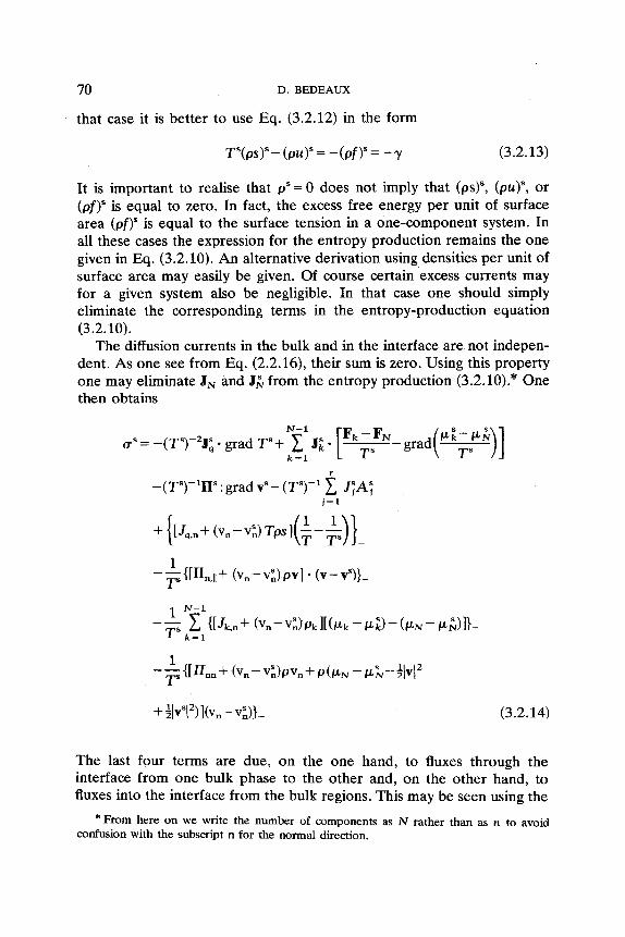
that case it is better to use Eq. (3.2.12) in the form
T"(ps)"- ( p ~ ) " = -(pf)"= -y (3.2.13)
It is important to realise that p s = 0 does not imply that (ps)", (pu)", or (pf)" is equal to zero. In fact, the excess free energy per unit of surface area (pf)" is equal to the surface tension in a one-component system. In all these cases the expression for the entropy production remains the one given in Eq. (3.2.10). An alternative derivation using densities per unit of surface area may easily be given. Of course certain excess currents may for a given system also be negligible. In that case one should simply eliminate the corresponding terms in the entropy-production equation (3.2.10).
The diffusion currents in the bulk and in the interface are not indepen- dent. As one see from Eq. (2.2.16), their sum is zero. Using this property one may eliminate J N and Jh from the entropy production (3.2.10).* One then obtains
N-1
us= - ( T p 2 J ; - grad T s + 1 J i - k = l
r
-( T")-W : grad vs - ( TS)-' 1 JsAs j = 1
1
The last four terms are due, on the one hand, to fluxes through the interface from one bulk phase to the other and, on the other hand, to fluxes into the interface from the bulk regions. This may be seen using the
*From here on we write the number of components as N rather than as n to avoid confusion with the subscript n for the normal direction.
NONEQUILIBRIUM THERMODYNAMICS AND STATISTICAL PHYSICS 71
identity
[ ab]- = a+b- + a-b, (3.2.15)
where the average of the bulk fields at the dividing surface, a+, is defined by
With the above identity one may, for example, write the contribution due to the heat current as the sum of two terms:
The first term is due to the heat current between the two bulk phases and the second is due to the heat current into the interface; the conjugate forces are ( l /T++ l / T ) and [(l/T)+- 1/77, respectively. One may re- write the last three terms as sums of two contributions in a similar way.
N THE PHENOMENOLOGICAL EQUATIONS
A. Introduction
If the system is in equilibrium, the entropy production is zero. This is the case if the thermodynamic forces are zero. As a result, the fluxes are also zero. Sufficiently close to equilibrium, the fluxes are linear functions of the thermodynamic forces. For a large class of irreversible phenomena these linear relations are in fact sufficient. The linear constitutive coeffi- cients will in general depend on the local values of the variables. Thus a coefficient like the viscosity depends on the temperature, and if the temperature is not uniform, neither is the viscosity. The resulting depen- dence on the local variables of the fluxes may in fact be nonlinear. As such there is a crucial difference from the linear dependence of the fluxes on the thermodynamic forces. These thermodynamic forces result from variation of the variables over a distance of a typical bulk correlation length. It is crucial for the hypothesis of local equilibrium that the variation over such distances be small. As a consequence, the linear dependence is already implicit in this hypothesis. The affinities of the chemical reactions are an exception in this context, because they depend
72 D. BEDEAUX
only on the values of variables in the same cell with a diameter of a bulk correlation length; here the hypothesis of local equilibrium implies that the reactions are slow compared with the time the cell needs to reach equilibrium. Though for chemical reactions also the reaction rates will be linear functions of the affinities if the system is sufficiently close to equilibrium, one must usually use nonlinear relations. These nonlinear relations are, as is clear from the discussion above, in agreement with the hypothesis of local equilibrium.
It should be emphasized that linear constitutive relations do not lead to linear equations of motion. Because of convection and the nonlinear nature of the equation of state, the equations of motion are in general highly nonlinear. The fully linearized equations play an important role in some problems, as, for example, in the description of fluctuations around equilibrium.
B. The Curie Symmetry Principle
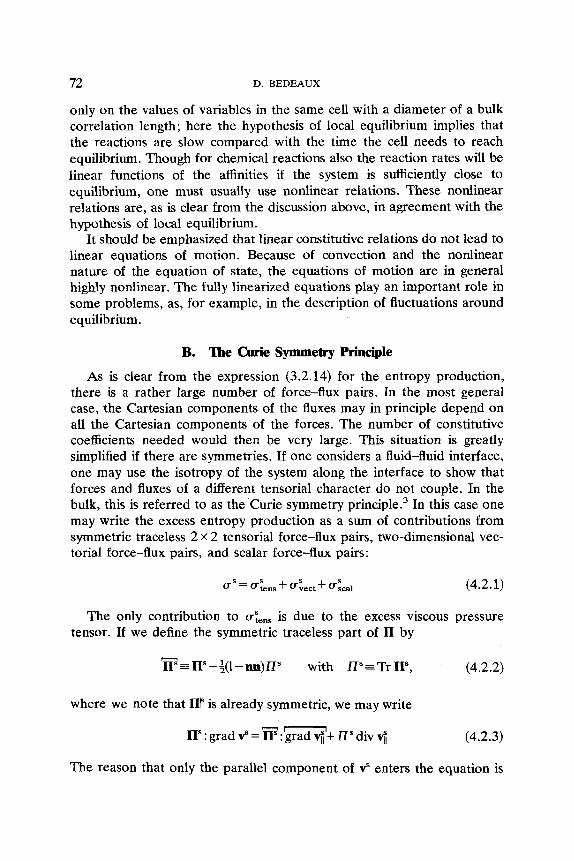
As is clear from the expression (3.2.14) for the entropy production, there is a rather large number of force-flux pairs. In the most general case, the Cartesian components of the fluxes may in principle depend on all the Cartesian components of the forces. The number of constitutive coefficients needed would then be very large. This situation is greatly simplified if there are symmetries. If one considers a fluid-fluid interface, one may use the isotropy of the system along the interface to show that forces and fluxes of a different tensorial character do not couple. In the bulk, this is referred to as the Curie symmetry pr in~iple .~ In this case one may write the excess entropy production as a sum of contributions from symmetric traceless 2 x 2 tensorial force-flux pairs, two-dimensional vec- torial force-flux pairs, and scalar force-flux pairs:
The only contribution to uiens is due to the excess viscous pressure tensor. If we define the symmetric traceless part of II by
where we note that IIP is already symmetric, we may write
n':gradv"=h":'gradflkn'div$ (4.2.3)
The reason that only the parallel component of v" enters the equation is
NONEQUILIBRIUM THERMODYNAMICS AND STATISTICAL PHYSICS 73
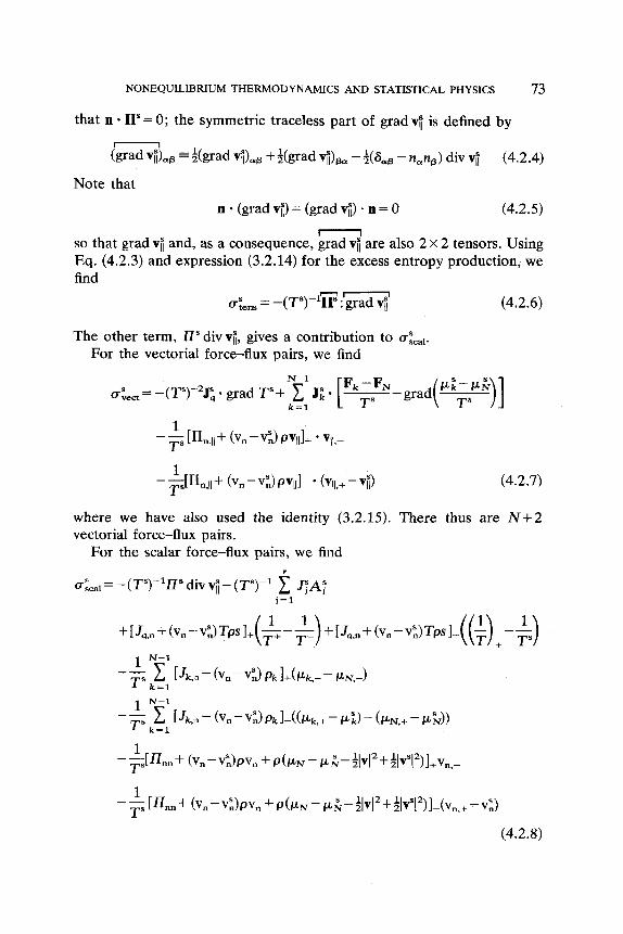
that n - II"= 0; the symmetric traceless part of grad vfi is defined by
(grad vSjmP =&grad v&p +;(grad vi)Pm - $(Sap - n,n,) div vi (4.2.4)
Note that
n * (grad vi) = (grad vfi) - n = 0 (4.2.5) - so that grad vi and, as a consequence, grad vi are also 2 x 2 tensors. Using Eq. (4.2.3) and expression (3.2.14) for the excess entropy production, we find
(4.2.6) usern = -(T s ) -1- IIs?grad 9'
The other term, Dsdivvfi, gives a contribution to u:&. For the vectorial force-flux pairs, we find
where we have also used the identity (3.2.15). There thus are N + 2 vectorial force-flux pairs.
For the scalar force-flux pairs, we find r
uLd = -(Ts)-117s div vfi- (T")-' 2 JsA; i = l
74 D. BEDEAUX
where we have again used the identity (3.2.15). We thus have 3 + r + N scalar force-flux pairs.
It is good to realize that isotropy of the interfacial region differs from isotropy in the bulk phases. In the bulk phase the isotropy implies that the properties of the system are not dependent on the direction. For the interface, isotropy implies that the properties do not depend on the directions along the interface. The properties in the direction orthogonal to the interface are clearly very different, however. The isotropy in the bulk regions is three-dimensional. The isotropy of the interface, which is described as a two-dimensional structure, is two-dimensional. The relev- ant tensors and vectors describing excess flows and forces along the interface are in fact two-dimensional. Because the interface is, of course, embedded in a three-dimensional space, a two-dimensional excess vector flow is written as a three-dimensional vector flow with a zero normal component; similarly one writes the 2 x 2 dimensional tensors as 3 x 3 tensors with five elements that are zero. Whereas the situation for the excess fluxes is reasonably self evident, this is less true of the extrapolated values of the bulk fluxes at the dividing surface. These extrapolated values are given by the usual three-dimensional isotropic linear laws in terms of the extrapolated bulk forces. A complete specification of the dynamical behavior of the bulk phase requires specifying the normal component of this extrapolated flux at the dividing surface, It is this normal component that appears in the excess entropy production. In this specification it becomes important to realize the two-dimensional isotropy of the interface. This results, for example, in the extrapolated values of the normal components of the heat flow and the diffusion flow being scalar in this context. As a consequence, diffusion through the interface may be driven by a finite value of one of the affinities. This process is called active t ran~por t .~ Similarly, extrapolated values of the viscous pressure tensor give the viscous forces of the bulk phases on the dividing surface. The parallel component of this viscous force, JI,,,,, is a two-dimensional vector and contributes to (+:ect, while the normal compo- nent of this force, ITn,, is a scalar and contributes to rid. A consequence of the symmetry breaking in the direction normal to the interface is that many cross effects exist that are impossible in the bulk regions. We shall return to these possibilities in the following sections, where we give the linear constitutive equations.
C. The Onsager Relations
There is one more symmetry property that reduces the number of independent linear constitutive coefficients. This property gives the so-
NONEQUILIBRIUM THERMODYNAMICS AND STATISTICAL PHYSICS 75
called Onsager relations between the linear coefficients describing cross effects, which are based on the time-reversal invariance of the micro- scopic equations of, motion. We refer the reader to de Groot and Mazur3 for a detailed discussion of the Onsager relations. In the following sections we shall simply give the explicit expressions in the various cases.
D. Symmetric Traceless Tensorial Force-Flux Pairs
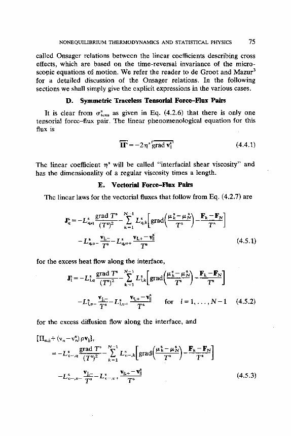
It is clear from as,, as given in Eq. (4.2.6) that there is only one tensorial force-flux pair. The linear phenomenological equation for this flux is
(4.4.1)
The linear coefficient q s will be called "interfacial shear viscosity" and has the dimensionality of a regular viscosity times a length.
E. Vectorial Force-Flux Pairs
The linear laws for the vectorial fluxes that follow from Eq. (4.2.7) are
grad T" N-l
(4.5.1)
for the excess heat flow along the interface,
-L;*u- %- T" LL+ - vr+-vi for 1=1,. . . , i V - l (4.5.2) T"
for the excess diffusion flow along the interface, and
(4.5.3)
76 D. BEDEAUX
and
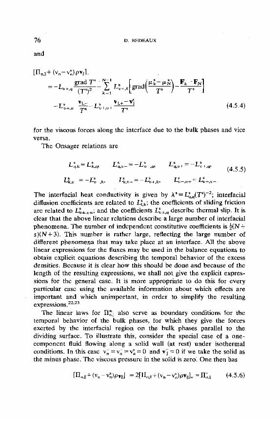
(4.5.4)
for the viscous forces along the interface due to the bulk phases and vice versa.
The Onsager relations are
L i , u - = - G - , k , Lsk,v+= -L:+,k, L:-,u+ L:+,v-
The interfacial heat conductivity is given by A"= L&JT")-'; interfacial diffusion coefficients are related to Li,k; the coefficients of sliding friction are related to L:*,v*; and the coefficients I&q describe thermal slip. It is clear that the above linear relations describe a large number of interfacial phenomena. The number of independent constitutive coefficients is $(N + s ) ( N + 3 ) . This number is rather large, reflecting the large number of different phenomena that may take place at an interface. All the above linear expressions for the fluxes may be used in the balance equations to obtain explicit equations describing the temporal behavior of the excess densities. Because it is clear how this should be done and because of the length of the resulting expressions, we shall not give the explicit expres- sions for the general case. It is more appropriate to do this for every particular case using the available information about which effects are important and which unimportant, in order to simplify the resulting expres~ions.''*'~
The linear laws for II;,,, also serve as boundary conditions for the temporal behavior of the bulk phases, for which they give the forces exerted by the interfacial region on the bulk phases parallel to the dividing surface. To illustrate this, consider the special case of a one- component fluid flowing along a solid wall (at rest) under isothermal conditions. In this case v; = v,' = vS, = 0 and v j = 0 if we take the solid as the minus phase. The viscous pressure in the solid is zero: One then has
NONEQUILIBRIUM THERMODYNAMICS AND STATISTICAL PHYSICS 77
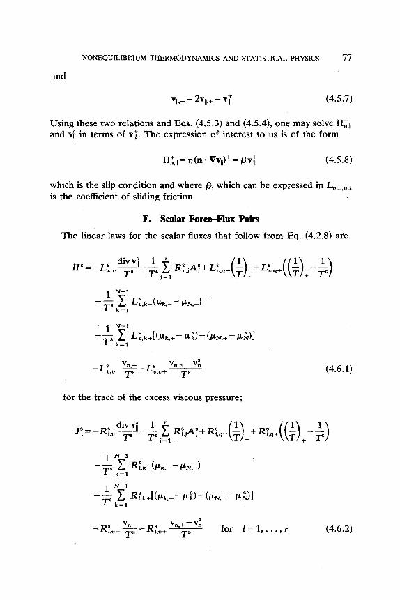
and
Using these two relations and Eqs. (4.5.3) and (4.5.4), one may solve II$l and vfi in terms of vt. The expression of interest to us is of the form
which is the slip condition and where a, which can be expressed in Lu*,v* is the coefficient of sliding friction.
F. Scalar Force-Flux Pairs
The linear laws for the scalar fluxes that follow from Eq. (4.2.8) are
(4.6.1)
for the trace of the excess viscous pressure;
(4.6.2)
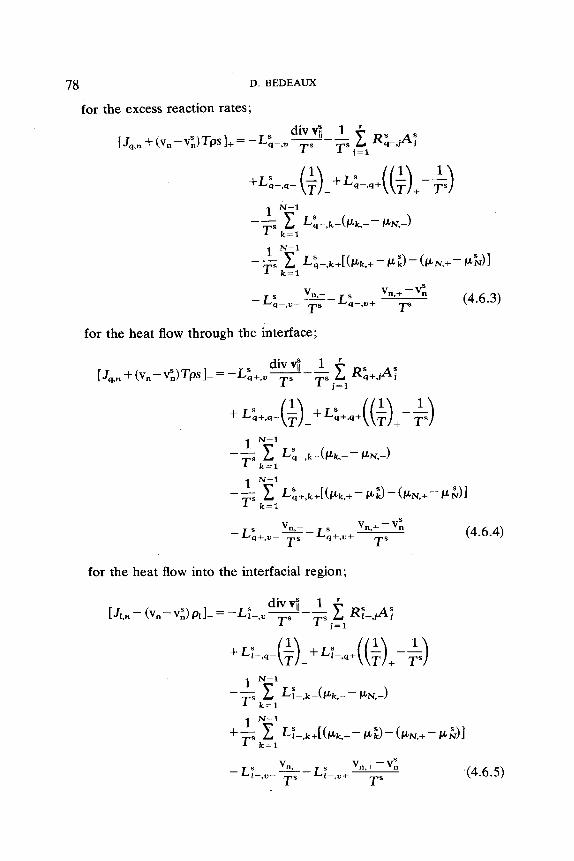
78 D. BEDEAUX
for the excess reaction rates;
(4.6.3) Vn,- vn,+ - vS, - L L v - T"- LSq-.Ll+ T"
for the heat flow through the interface;
(4.6.4) Vn,- vn,+ - v: T" LSq+,v+- T S
- L",,,- --
for the heat flow into the interfacial region;
(4.6.5)
NONEQUILIBKIUM THERMODYNAMICS AND STATISTICAL PHYSICS 79
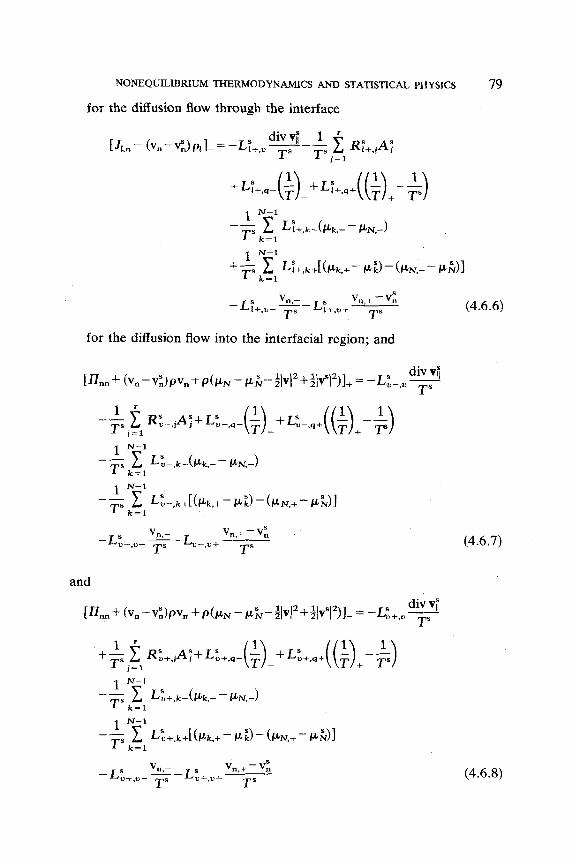
for the diffusion flow through the interface
for the diffusion flow into the interfacial region; and
(4.6.7)
(4.6.8)
80 D. BEDEAUX
for the normal components of the viscous forces on the interface due to the bulk phases and vice versa.
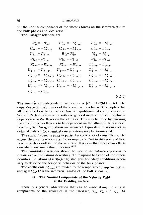
The Onsager relations are
(4.6.9)
The number of independent coefficients is i(3 + r + N)(4 + I + N ) . The dependence on the affinities of the above fluxes is linear. This implies that all reactions have to be rather close to equilibrium. As we discussed in Section 1V.A it is consistent with the general method to use a nonlinear dependence of the fluxes on the affinities. This may be done by choosing the constitutive coefficients to be dependent on the affinities. In that case, however, the Onsager relations are incorrect. Equivalent relations such as detailed balance for chemical rate equations may be formulated.
The scalar force-flux pairs in particular show a lot of cross effects. The excess chemical reactions are, for example, coupled to diffusion and heat flow through as well as into the interface. It is clear that these cross effects describe many interesting p r o c e ~ s e s . ~ . ~ ~
The constitutive relations should be used in the balance equations to obtain explicit equations describing the temporal behavior of the excess densities. Equations (4.6.3)-(4.6.8) also give boundary conditions neces- sary to describe the temporal behavior of the bulk phases.
The coefficients L",,,, are related to the temperature jump coefficient, and qi= L",,/T is the interfacial analog of the bulk viscosity.
G. The Normal Components of the Velocity Field at the Dividing Surface
There is a general observation that can be made about the normal components of the velocities at the interface, v;,, vz, and v;,. At
NONEQUILIBRIUM THERMODYNAMICS AND STATISTICAL PHYSICS 81
equilibrium these velocities are clearly equal to zero. If the system is not in equilibrium these normal velocities will be finite and in general will no longer be equal to each other. Under most conditions the dissipative fluxes given by the linear laws in the preceding paragraphs are relatively small. This implies that the convective contributions in the reference frame of the dividing surface will usually also be small. Thus, for example. [(v,-v:)Tps], is usually small. In view of the fact that the entropy density difference (the latent heat) is usually not small, one may conclude that in most cases the normal components of the velocities at the dividing surface are almost equal:24
(4.7.1)
The importance of the latent heat in the theory of n~cleation,'~ where it leads to growth instabilities and pattern
There are, of course, also phenomena in which the velocities differ considerably. One example is a shock wave, in which the latent heat may lead to such a high temperature in the shock front that it starts fires.27 Another example is explosive crystallization.28
Clearly not only the heat flux but also other fluxes of densities that differ sufficiently in the two phases lead to Eq. (4.7.1) in most cases
is related to this.
H. The Liquid-Vapor Interface
To show how one obtains differential equations for the temporal behavior of the excess densities and the location of the interface, we shall discuss this procedure for the special case of a liquid-vapor interface in a one-component system." In the following sections, we shall also consider both the equilibrium and the nonequilibrium fluctuations of this system in more detail.
We shall further simplify this discussion by considering only small deviations from the equilibrium state and by fully linearizing the equa- tions. As the force on the system, we use a gravitational force along the z axis,
IF = -grad 9 = - g(0, 0 , l ) e + = gz (4.8.1)
The equilibrium dividing surface is assumed to be planar, which is adequate for a large container, and is chosen to coincide with the xy plane. At equilibrium all velocities and other fluxes are zero. Equation (2.4.1) gives for the pressure in the bulk regions
a a - p,',(z> := -gp,',(z) and -pi&) = - g p & ( z ) (4.8.2) az 82
82 D. BEDEAUX
while Eq. (2.4.6) gives as the jump in the pressure at the dividing surface
(4.8.3) - s Peq,- - -Peqg
The surface tension is clearly constant and equal to its equilibrium value [cf. Eq. (2.4.9)]. Because the thermodynamic forces in the entropy production both in the bulk regions [Eq. (3.2.7)], and at the interface [Eq. (3.2.10)] must all be zero at equilibrium, we have
where po is the chemical potential for z = 0. Linearizing Eq. (2.2.10) around equilibrium, we find
a - 6p" = --piq div v" - [ peq(v, - v",)l- a t
(4.8.5)
A deviation from the equilibrium value will be indicated by the prefactor 6. Similarly, we find for the interfacial velocity field, after linearizing Eq. (2.4.6) and using Eqs. (2.4.7) and (4.8.3),
a at
pEq- vs= -VSy-(Cyeq+6p-+g6ps)neq= gpE,6n-neq.n-
(4.8.6)
Here we have used the equilibrium expressions for the curvature and the normal:
C,, = 0 and ne, = (0, 0 , l ) (4.8.7)
Note that to linear order, both V8.y and Sn are in the x y plane, so that we find for the normal component v;, by contracting Eq. (4.8.6) with neq,
a PL, vs, = -Cyeq+6p-+g6p"-nn,n,- (4.8.8)
where we have used the facts that to linear order v; = vz and 17n,n = I&. We find for the parallel components
(4.8.9)
NONEQUILIBEUUM THERMODYNAMICS AND STATISTICAL PHYSICS 83
For the excess internal energy per unit surface area, we find on lineariza- tion of Eq. (2.5.5) and using Eq. (4.8.5)
To obtain more convenient expressions, we shall now use the freedom in the choice of the dividing surface and use
One usually refers to this choice as that made by Gibbs. In fact, he also mentioned the other possible choices.' Substitution of this definition in the above differential equations gives
s - P,',V,+ - P,V, [p,(v,-vj:)]-=O-+v,- + - Peq- Peq
(4.8.12)
SP- + 4 n , - = CYeq (linearized Laplace equation) (4.8.13)
The equation for the internal energy density remains the same. Notice that in view of the fact that we use Eq. (4.8.9), we have implicitly assumed that the excess mass flow is equal to zero, (pv)" = 0.
If we define the interfacial specific heat by
(4.8.15)
and use the fact that (pu)" is now a function of the temperature alone, we find the following equation for the interfacial temperature: l1
a cis -- ST" = -div J i - To(ps)Zq div v"
at
-TOSeq,-[Peq(Vn- v",) I+ - J q m (4.8.16)
To obtain this expression, we also used the thermodynamic relation
Ts(Ps)s = (up)"- Y (4.8.17)
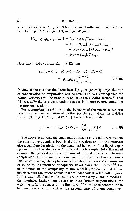
84 D. BEDEAUX
which follows from Eq. (3.2.12) for this case. Furthermore, we used the fact that Eqs. (3.2.12), (4.8.12), and (4.8.4) give
Note that it follows from Eq. (4.8.12) that
(4.8.18)
In view of the fact that the latent heat Toseq,- is generally large, the rate of condensation or evaporation will be small and as a consequence the normal velocities will be practically equal at the dividing surface.= That this is usually the case we already discussed in a more general context in the previous section.
For a complete description of the behavior of the interface, we also need the linearized equation of motion for the normal on the dividing surface [cf. Eqs. (1.2.30) and (2.2.7)], for which one finds
-8n=-(I-%,%,)-Vv;= a - (4.8.19) at
The above equations, the analogous equations in the bulk regions, and the constitutive equations both in the bulk regions and on the interface give a complete description of the dynamical behavior of the liquid-vapor system. It is clear that even for this relatively simple, fully linearized example the general solution in terms of normal modes is extremely complicated. Further simplifications have to be made and in such simp- lified cases one may study phenomena like the reflection and transmission of sound by the interface or capillary waves along the interface.23 The main source of the complexity of the general problem is that at the interface bulk excitations couple that are independent in the bulk regions. In this way bulk shear modes couple with, for example, sound modes at the interface. Rather than discussing these further simplifications, for which we refer the reader to the l i t e r a t ~ r e , ~ ~ * ~ ~ * ~ ~ we shall proceed in the following sections to consider the general case of a one-component
NONEQUILIHRIUM THERMODYNAMICS AND STATISTICAL PHYSICS 85
liquid-vapor interface and to discuss the equilibrium and the nonequilib- rium fluctuations.
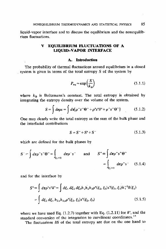
V EQUILIBRIUM FLUCTUATIONS OF A LIQUID-VAPOR INTERFACE
A. Introduction
The probability of thermal fluctuations around equilibrium in a closed system is given in terms of the total entropy S of the system by
(5.1.1)
where kB is Boltzmann's constant. The total entropy is obtained by integrating the entropy density over the volume of the system.
S = drps = dr[p-s-W+ psssSs+ p+s'O+] (5.1.2) I I One may clearly write the total entropy as the sum of the bulk phase and the interfacial contributions
s = s-+ S"+ s+
which are defined for the bulk phases by
(5.1.3)
(5.1.4)
and for the interface by
(5.1.5)
where we have used Eq. (1.2.7) together with Eq. (1.2.11) for S", and the standard conversion of the integration to curvilinear coordinate^.'^
The fluctuations 6s of the total entropy are due on the one hand to
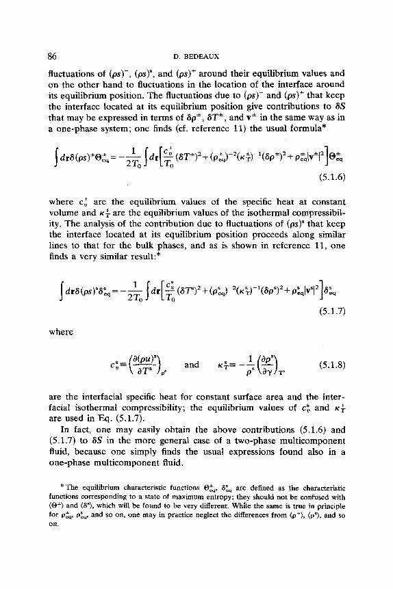
86 D. BEDEAUX
fluctuations of (ps ) - , (ps)", and (ps)' around their equilibrium values and on the other hand to fluctuations in the location of the interface around its equilibrium position. The fluctuations due to ( p s ) - and (ps)' that keep the interface located at its equilibrium position give contributions to SS that may be expressed in terms of S p * , ST*, and v* in the same way as in a one-phase system; one finds (cf. reference 11) the usual formula*
(5.1.6)
where c z are the equilibrium values of the specific heat at constant volume and K $ are the equilibrium values of the isothermal compressibil- ity. The analysis of the contribution due to fluctuations of (ps)" that keep the interface located at its equilibrium position proceeds along similar lines to that for the bulk phases, and as is shown in reference 11, one finds a very similar result:*
(5.1.7)
where
are the interfacial specific heat for constant surface area and the inter- facial isothermal compressibility; the equilibrium values of cS, and K $
are used in Eq. (5.1.7). In fact, one may easily obtain the above contributions (5.1.6) and
(5.1.7) to SS in the more general case of a two-phase multicomponent fluid, because one simply finds the usual expressions found also in a one-phase multicomponent fluid.
* The equilibrium characteristic functions @&, 8% are defined as the characteristic functions corresponding to a state of maximum entropy; they should not be confused with (0') and (8"), which will be found to be very different. While the same is true in principle for p&, p",, and so on, one may in practice neglect the differences from (p*), (p"), and so on.
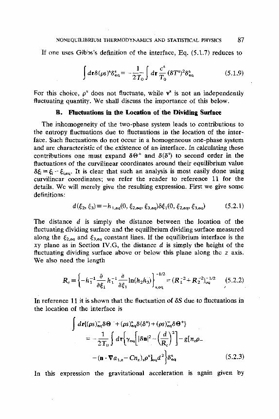
NONEQUILIBRIUM THERMODYNAMICS AND STATISTICAL PHYSICS 87
If one uses Gibbs’s definition of the interface, Eq. (5.1.7) reduces to
For this choice, ps does not fluctuate, while vs is not an independently fluctuating quantity. We shall discuss the importance of this below.
B. Fluctuations in the Location of the Dividing Surface
The inhomogent:ity of the two-phase system leads to contributions to the entropy fluctuations due to fluctuations in the location of the inter- face. Such fluctuations do not occur in a homogeneous one-phase system and are characteristic of the existence of an interface. In calculating these contributions one must expand SO” and S(Ss) to second order in the fluctuations of the curvilinear coordinates around their equilibrium value S t i 3 ti - It is clear that such an analysis is most easily done using curvilinear coordinates; we refer the reader to reference 11 for the details. We will merely give the resulting expression. First we give some definitions:
d (52, ‘53) E -hl,ea(O, SZ,eq, t3,eq)S51(09 52,eq, t3,eq) (5.2.1)
The distance d is simply the distance between the location of the fluctuating dividing surf ace and the equilibrium dividing surface measured along the (2,eq and &eq constant lines. If the equilibrium interface is the xy plane as in Section IV.G, the distance d is simply the height of the fluctuating dividing surface above or below this plane along the z axis. We also need the length
In reference 11 it is shown that the fluctuation of SS due to fluctuations in the location of the interface is
dr{(ps);qSO-+ (ps)~,G(S”) + (~S);~,SO’}
In this expression the gravitational acceleration is again given by
88 D. BEDEAUX
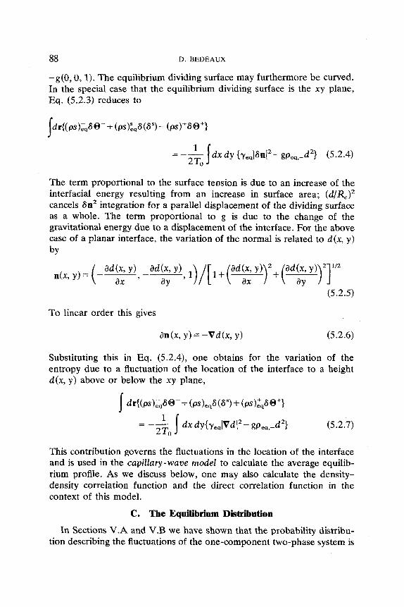
-g(O, 0, l) . The equilibrium dividing surface may furthermore be curved. In the special case that the equilibrium dividing surface is the xy plane, Eq. (5.2.3) reduces to
The term proportional to the surface tension is due to an increase of the interfacial energy resulting from an increase in surface area; (d/R)" cancels an2 integration for a parallel displacement of the dividing surface as a whole. The term proportional to g is due to the change of the gravitational energy due to a displacement of the interface. For the above case of a planar interface, the variation of the normal is related to d(x, y)
by
(5.2.5)
To linear order this gives
Substituting this in Eq. (5.2.4), one obtains for the variation of the entropy due to a fluctuation of the location of the interface to a height d(x, y) above or below the xy plane,
This contribution governs the fluctuations in the location of the interface and is used in the capillary-wave model to calculate the average equilib- rium profile. As we discuss below, one may also calculate the density- density correlation function and the direct correlation function in the context of this model.
C. The Equilibrium Distribution
In Sections V.A and V.B we have shown that the probability distribu- tion describing the fluctuations of the one-component two-phase system is
NONEQUILIBRIUM THERMODYNAMICS AND STATISTICAL PHYSICS 89
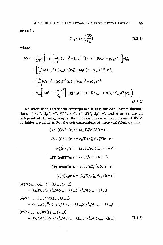
given by
P,=exp(E)
where
(5.3.1)
(5.3.2)
An interesting and useful consequence is that the equilibrium fluctua- tions of ST-, Sp- , v-, ST+, S p + , v+, S T , Sp”, vs, and d or 6n are all independent. In other words, the equilibrium cross correlations of these variables are all zero. For the self correlations of these variables, we find
(Xf-(r)ST-(r’)) = (kBTi/C,)S (r - r’)
(5.3.3)
90 D. BEDEAUX
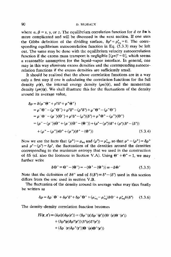
where a, 0 = x, y, or z . The equilibrium correlation function for d or Sn is more complicated and will be discussed in the next section. If one uses the Gibbs definition of the dividing surface, Sp"= pz,= 0. The corre- sponding equilibrium autocorrelation function in Eq. (5.3.3) may be left out. The same may be done with the equilibrium velocity autocorrelation function if the excess mass transport is negligible [ (pv)" = 01, which seems a reasonable assumption for the liquid-vapor interface. In general, one may in this way eliminate excess densities and the corresponding autocor- relation functions if the excess densities are sufficiently small.
It should be realized that the above correlation functions are in a way only a first step if one is calculating the correlation functions for the full density p(r), the internal energy density (pu)(r), and the momentum density (pv)(r). We shall illustrate this for the fluctuations of the density around its average value,
Sp = S ( p 3 - t pSSS+p+@+)
= p-@--(p-@-)+ p"6"-(pSSS)+ p+@+-(p+@+)
= p-@--(p-) (@-)+p"SS-(p")(6")+p+@+-(p+)(@+)
= (p - - (p - ) )@-+(p - ) (@- - (0-))+ (p"-(pS))GS+ (p") (SS- (SS) )
+ ( p + - ( p + ) ) ~ + + (p+)(e+ - (@+)I (5.3.4)
Now we use the facts that (p ' ) = pe4 and (p")- p",, so that p* - (p" ) = 6p* and ps- (p" ) = Sp", the fluctuations of the densities around the densities corresponding to the maximum entropy that we used in the construction of 6s (cf. also the footnote in Section V.A). Using @-+a+= 1, we may further write
6 0- EE 0- - (@-) = - (@+ - (0')) - @+ (5.3.5)
Note that the definition of SO" and of S ( S s ) = S s - ( S s ) used in this section differs from the one used in section V.B.
The fluctuation of the density around its average value may thus finally be written as
The density-density correlation function becomes
NONEQUILIBRIUM THERMODYNAMICS AND STATISTICAL PHYSICS 91
+ ([(Pi,(d - P:,(m@-b) + P:,(r)6(wr>>l x [(piq(r’) - dq(r’))6@-(r? + pZq(r’)Ws(r’))l)
+ (p,+,(r))’(0+(r))~~l6(r-r’)
+ ( [ (P&) - P:q(r))8@-(r) + P~,(r)6(Gs(r))I[fP~,(r’) - p&(r’))6@-kr) + pE4(r”W(r))I)
= k BTo[(Piq (r))’(@-(I))K T + (p$(r))2(8s(r>>K .S-
(5.3.7)
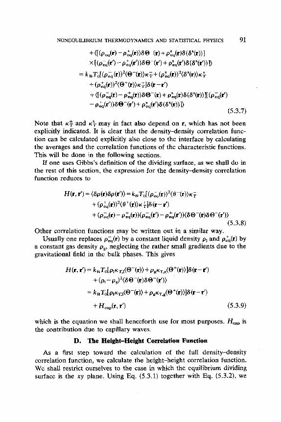
Note that K $ and K; may in fact also depend on r, which has not been explicitly indicated. It is clear that the density-density correlation func- tion can be calculated explicitly also close to the interface by calculating the averages and the correlation functions of the characteristic functions. This will be done in the following sections.
If one uses Gibbs’s definition of the dividing surface, as we shall do in the rest of this sect ion, the expression for the density-density correlation function reduces to
H(r , r’) = (6p(r)6p(r’)) = ksT,[(P,(r))’(e-(r))K,
+ (~&(r>)”(e+(r)>~”T16 (r - r’)
+ (piq(r> - dqWb;,(r’) - dq( r r ) ) (6 @-(rM @-(r’)> (5.3.8)
Other correlation functions may be written out in a similar way. Usually one replaces p;,(r) by a constant liquid density p1 and p&(r) by
a constant gas density pg, neglecting the rather small gradients due to the gravitational field in the bulk phases. This gives
(5.3.9)
which is the equation we shall henceforth use for most purposes. Hap is the contribution due to capillary waves.
D. The Height-Height Correlation Function
As a first step toward the calculation of the full density-density correlation function, we calculate the height-height correlation function. We shall restrict ourselves to the case in which the equilibrium dividing surface is the xy plane. Using Eq. (5.3.1) together with Eq. (5.3.2), we
92 D. BEDEAUX
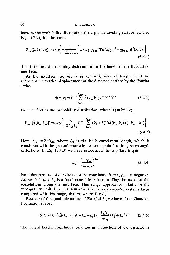
have as the probability distribution for a planar dividing surface [cf. also Eq. (5.2.7)] for this case
(5.4.1)
This is the usual probability distribution for the height of the fluctuating interface.
As the interface, we use a square with sides of length L. If we represent the vertical displacement of the distorted surface by the Fourier series
k."a
k.k,
d(x, y ) = L-2 1 d(k,, k,) ei(k=x+kyy) (5.4.2)
then we find as the probability distribution, where k$= k,2 i k:,
(5.4.3)
Here k,,= 27r/&, where TB is the bulk correlation length, which is consistent with the general restriction of our method to long-wavelength distortions. In Eq. (5.4.3) we have introduced the capillary length
(5.4.4)
Note that because of our choice of the coordinate frame, pq,- is negative. As we shall see, L, is a fundamental length controlling the range of the correlations along the interface. This range approaches infinite in the zero-gravity limit. In our analysis we shall always consider systems large compared with this range, that is, where L >> L,.
Because of the quadratic nature of Q. (5.4.3), we have, from Gaussian fluctuation theory,
S ( k ) = K 2 ( d ( k , , ky )d ( -kx , -k,)) = (kf+L;2)-1 (5.4.5) Yeq
The height-height correlation function as a function of the distance is
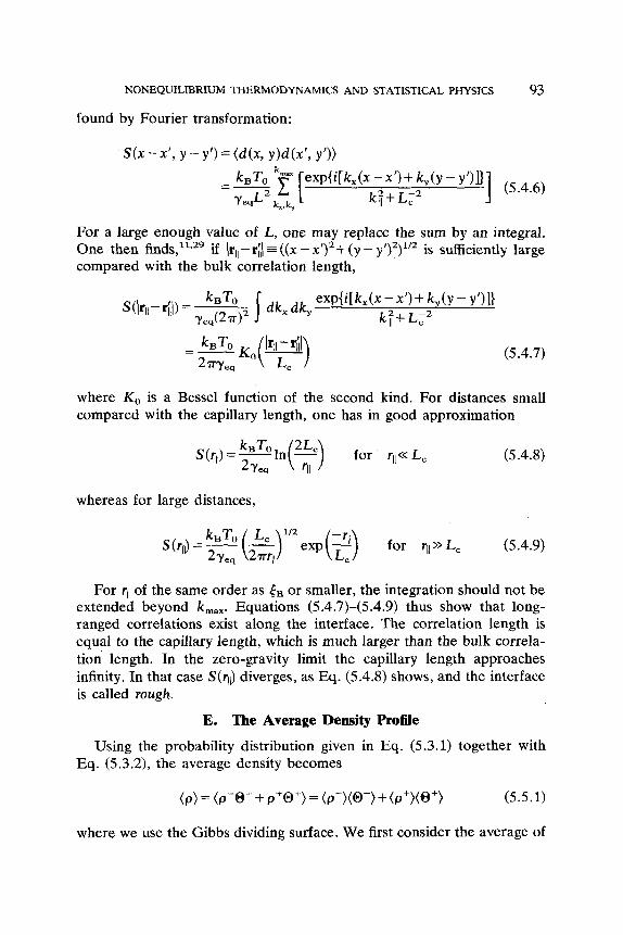
NONEQUILIBRIUM THERMODYNAMICS AND STATISTICAL PHYSICS 93 ’
found by Fourier transformation:
] (5.4.6) exp{i[k,(x-x’)+k,(y-y’)])
k i + L i 2
For a large enough value of L, one may replace the sum by an integral. One then if lrl,-ril = ((x - x ’ ) ~ + (y - Y ’ ) ~ ) ” ~ is sufficiently large compared with the bulk correlation length,
(5.4.7)
where KO is a compared with
Bessel function of the second kind. For distances small the capillary length, one has in good approximation
(5.4.8)
whereas for large distances,
For rll of the same order as & or smaller, the integration should not be extended beyond kmm. Equations (5.4.7)-(5.4.9) thus show that long- ranged correlations exist along the interface. The correlation length is equal to the capillary length, which is much larger than the bulk correla- tion length. In the zero-gravity limit the capillary length approaches infinity. In that case S(rlJ diverges, as Eq. (5.4.8) shows, and the interface is called rough.
E. The Average Density Profile
Using the probability distribution given in Eq. (5.3.1) together with Eq. (5.3.2), the average density becomes
where we use the Gibbs dividing surface. We first consider the average of
94 D. BEDEAUX
the characteristic functions,
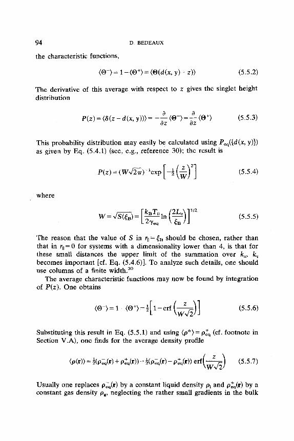
(W) = 1 -(a+) = (O(d(x, y ) - z)) (5.5.2)
The derivative of this average with respect to z gives the singlet height distribution
(5.5.3)
This probability distribution may easily be calculated using P,({d (x, y)}) as given by Eq. (5.4.1) (see, e.g., reference 30); the result is
where
112
(5.5.4)
(5.5.5)
The reason that the value of S in rII = tB should be chosen, rather than that in rll= 0 for systems with a dimensionality lower than 4, is that for these small distances the upper limit of the summation over k,, k, becomes important [cf. Eq. (5.4.6)]. To analyze such details, one should use columns of a finite
The average characteristic functions may now be found by integration of P ( z ) . One obtains
(5.5.6)
Substituting this result in Eq. (5.5.1) and using (p') = p & (cf. footnote in Section V.A), one finds for the average density profile
Usually one replaces pZq(r) by a constant liquid density p, and pt(r) by a constant gas density ps, neglecting the rather small gradients in the bulk
NONEQUILIERIUM THERMODYNAMICS AND STATISTICAL PHYSICS 95
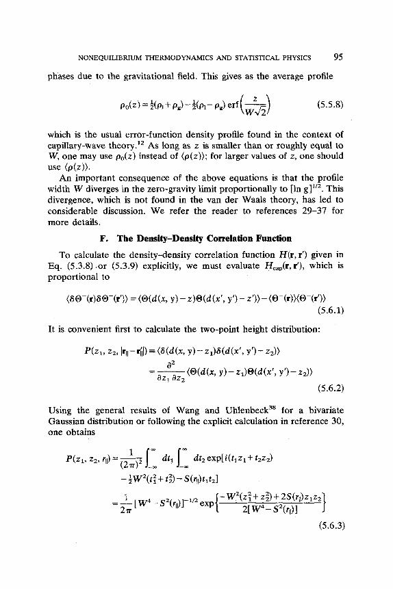
phases due to the gravitational field. This gives as the average profile
(5.5.8)
which is the usual error-function density profile found in the context of capillary-wave theory.12 As long as z is smaller than or roughly equal to W, one may use p&) instead of (p(z) ) ; for larger values of z, one should
An important consequence of the above equations is that the profile width W diverges in the zero-gravity limit proportionally to [In g]1’2. This divergence, which is not found in the van der Waals theory, has led to considerable discussion. We refer the reader to references 29-37 for more details.
use ( ~ ( z ) ) .
F. The Density-Density Correlation Function
To calculate the: density-density correlation function H(r, r’) given in Eq. (5.3.8) .or (5.:3.9) explicitly, we must evaluate HC&, r‘), which is proportional to
(8W(r)8@-(rf)) = (O(d(x, y) - z)O(d(x‘ , y’) - 2‘))- (O-(r))(W(r’)) (5.6.1)
It is convenient first to calculate the two-point height distribution:
Using the general results of Wang and U h l e n b e ~ k ~ ~ for a bivariate Gaussian distribution or following the explicit calculation in reference 30, one obtains
- ;w2ct:+ 6)- S(q,)t1t2]
(5.6.3)
96 D. BEDEAUX
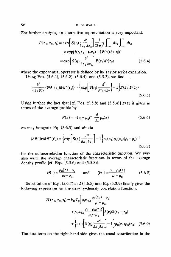
For further analysis, an alternative representation is very important:
(5.6.4)
where the exponential operator is defined by its Taylor series expansion. Using Eqs. (5.6.1), (5.6.2), (5.6.4), and (5.5.3), we find
(5.6.5)
Using further the fact that [cf. Eqs. (5.5.8) and (5.5.4)] P(z) is given in terms of the average profile by
(5.6.6) d
P(Z) = -(PI- Pg)-l-& P o ( Z )
we may integrate Eq. (5.6.5) and obtain
(8@3)8@-(r’)> = p0(z1)po(z2)(pI- pg)-’
(5.6.7)
for the autocorrelation function of the characteristic function. We may also write the average characteristic functions in terms of the average density profile [cf. Eqs. (5.5.6) and (5.581:
Substitution of Eqs. (5.6.7) and (5.6.8) into Eq. (5.3.9) finally gives the following expression for the density-density correlation function:
The first term on the right-hand side gives the usual contribution in the
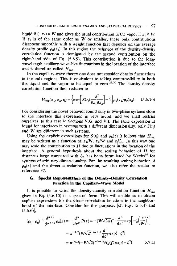
NONEQUILIBRIUM THERMODYNAMICS AND STATISTICAL PHYSICS 97
liquid if (-zl) >> W and gives the usual contribution in the vapor if z1 >> W. If z1 is of the same order as W or smaller, these bulk contributions disappear smoothly with a weight function that depends on the average density profile po(zl). In this region the behavior of the density-density correlation function is dominated by the second contribution on the right-hand side of Eq. (5.6.9). This contribution is due to the long- wavelength capillary-wave-like fluctuations in the location of the interface and is therefore called H,.
In the capillary-wave theory one does not consider density fluctuations in the bulk regions. This is equivalent to taking compressibility in both the liquid and the vapor to be equal to The density-density correlation function then reduces to
For considering the novel behavior found only in two-phase systems close to the interface this expression is very useful, and we shall restrict ourselves to this case in Sections V.G. and V.I. The same expression is found for interfaces in systems with a different dimensionality; only S(rll) and W are different in such systems.
Using the explicit expressions for S(ri,) and po(z) it follows that Hap may be written as a function of zl/W, zz/W and q/LC. In this way one may scale the contribution to H due to fluctuations in the location of the interface. A general hypothesis about the scaling behavior of H for distances large compared with & has been formulated by Weeks36 for systems of arbitrary dimensionality. For the resulting scaling behavior of po(z) and the direct correlation function, we also refer the reader to reference 37.
G. Special Representation of the Density-Density Correlation Function in the Capillary-Wave Model
It is possible to write the density-density correlation function Heap given in Eq. (5.6.10) in a spectral form. This will enable us to obtain explicit expressions for the direct correlation functions in the neighbar- hood of the interface. Consider for this purpose, [cf. Eqs. (5.5.4) and (5.6.6)1,
= T-~"(- W&)-(n+l)Hn(J) exp(- S2) (5.7.1)
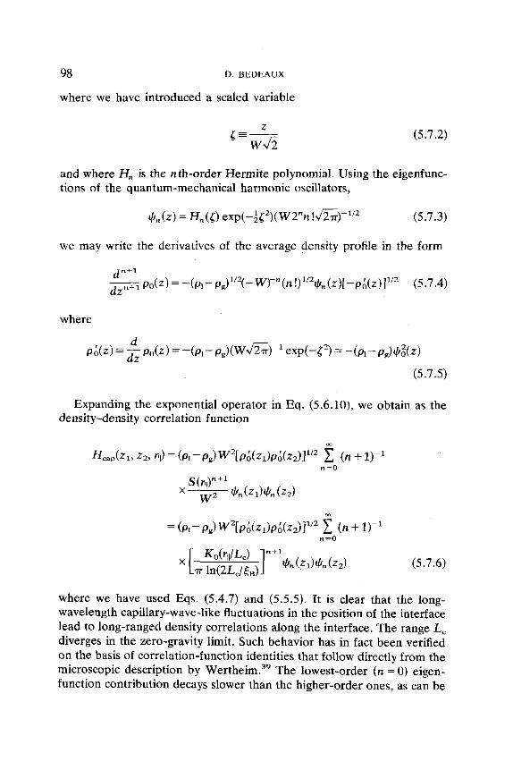
98 D. BEDEAUX
where we have introduced a scaled variable
z c=- W J Z
(5.7.2)
and where H,, is the n th-order Hermite polynomial. Using the eigenfunc- tions of the quantum-mechanical harmonic oscillators,
we may write the derivatives of the average density profile in the form
where
Expanding the exponential operator in Eq. (5.6.10), we obtain as the density-density correlation function
(5.7.6)
where we have used Eqs. (5.4.7) and (5.5.5). It is clear that the long- wavelength capillary-wave-like fluctuations in the position of the interface lead to long-ranged density correlations along the interface. The range L, diverges in the zero-gravity limit. Such behavior has in fact been verified on the basis of correlation-function identities that follow directly from the microscopic description by Wertheim.39 The lowest-order ( n = 0) eigen- function contribution decays slower than the higher-order ones, as can be
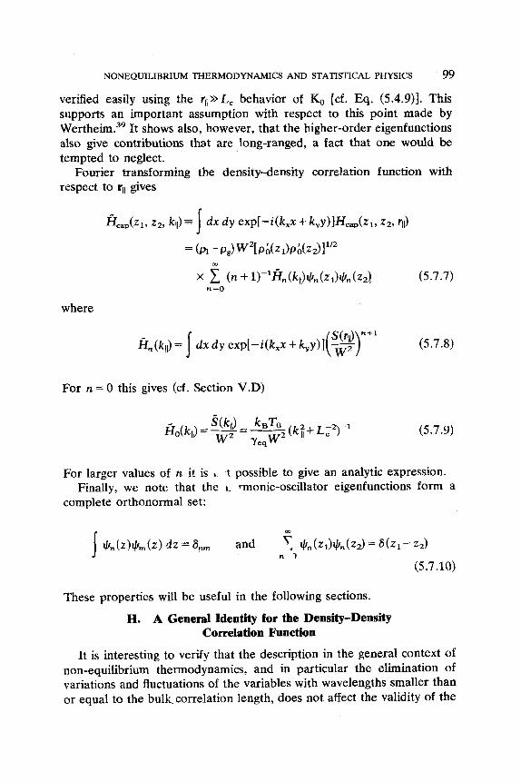
NONEQUILIHRIUM THERMODYNAMICS AND STATISTICAL PHYSICS 99
verified easily using the rll>>L, behavior of KO [cf. Eq. (5.4.9)]. This supports an important assumption with respect to this point made by W e r t h e h ~ . ~ ~ It shows also, however, that the higher-order eigenfunctions also give contributions that are long-ranged, a fact that one would be tempted to neglect.
Fourier transforming the density-density correlation function with respect to rll gives
fiap(z~, z2, kll) = 5 dx dy exp[--i(k,x + ky~)lH,p(zl, 22, q)
= (PI- P3w2[P~(21)P~(~2>1”2 m
x C (n + l ) - l ~ n ( k , , ) + n ( Z l ) + n ( z * ~ (5.7.7) n =O
where
For n = 0 this gives (cf. Section V.D)
(5.7.9)
For larger values of n it is
complete orthonormal set:
t possible to give an analytic expression. Finally, we note that the I. monic-oscillator eigenfunctions form a
These properties will be useful in the following sections.
H. A General Identity for the Density-Density Correlation Function
It is interesting to verify that the description in the general context of non-equilibrium thermodynamics, and in particular the elimination of variations and fluctuations of the variables with wavelengths smaller than or equal to the bulk,correlation length, does not affect the validity of the
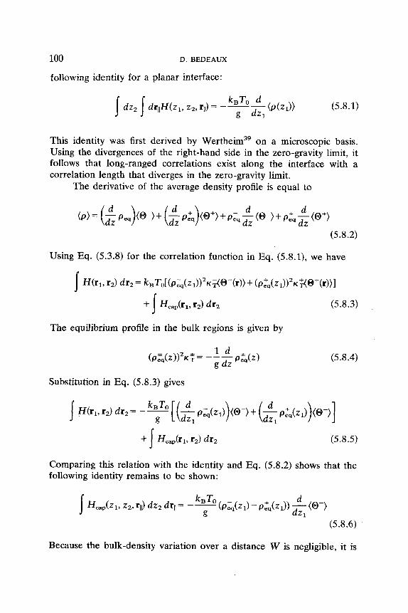
100 D. BEDEAUX
following identity for a planar interface:
This identity was first derived by W e r t h e i ~ n ~ ~ on a microscopic basis. Using the divergences of the right-hand side in the zero-gravity limit, it follows that long-ranged correlations exist along the interface with a correlation length that diverges in the zero-gravity limit.
The derivative of the average density profile is equal to
(5.8.2)
Using Eq. (5.3.8) for the correlation function in Eq. (5.8.1), we have
I ff(ri, f2) drz = k ~ T ~ [ ( ~ ~ q ( Z i ) ) ~ K ~ @ - ( r ) ) + ( P , ' , ( z ~ ) ) ~ K ~ @ + ( r ) ) l
+ Hcap(rl, r2) dr2 (5.8.3)
The equilibrium profile in the bulk regions is given by
(5.8.4)
Substitution in Eq. (5.8.3) gives
Comparing this relation with the identity and Eq. (5.8.2) shows that the following identity remains to be shown:
Because the bulk-density variation over a distance W is negligible, it is
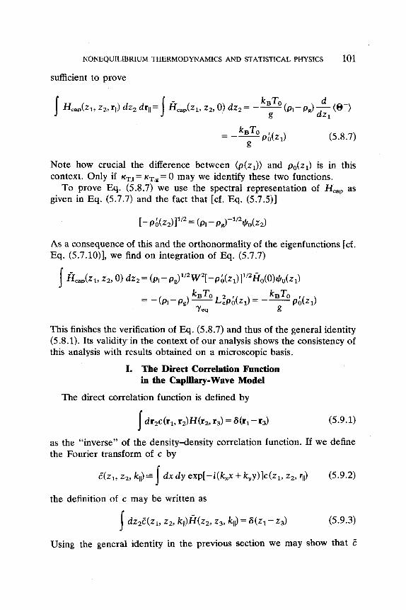
NONEQUILIBRIUM THERMODYNAMICS AND STATISTICAL PHYSICS 101
sufficient to prove
(5.8.7)
Note how crucial the difference between (p(zl)) and po(zl) is in this context. Only if K T , ~ = K T , ~ = 0 may we identify these two functions.
To prove Eq. (5.8.7) we use the spectral representation of Heap as given in Eq. (5.7.7) and the fact that [cf. Eq. (5.7.5)]
As a consequence of this and the orthonormality of the eigenfunctions [cf. Eq. (5.7.10)], we find on integration of Eq. (5.7.7)
This finishes the verification of Eq. (5.8.7) and thus of the general identity (5.8.1). Its validity in the context of our analysis shows the consistency of this analysis with results obtained on a microscopic basis.
I. The Direct Correlation Function in the Capillary-Wave Model
The direct correlation function is defined by
d r2c(rl, r2)H(r2, r3) = 8 (rl - G) (5.9.1)
as the “inverse” of the density-density correlation function. If we define the Fourier transform of c by
c‘(zl, z2, kll)= dxdy exp[-i(k,x+ k,y)]c(zl, z,, rll) (5.9.2) J the definition of c may be written as
j dzzE(z1, 22, kll)mz,, 2% kll) = a h - 23) (5.9.3)
Using the general identity in the previous section we may show that E
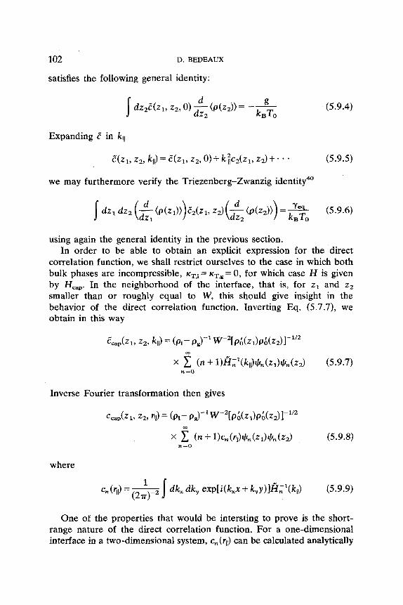
102 D. BEDEAUX
satisfies the following general identity:
Expanding c' in kll
(5.9.4)
we may furthermore verify the Triezenberg-Zwanzig identity4'
using again the general identity in the previous section. In order to be able to obtain an explicit expression for the direct
correlation function, we shall restrict ourselves to the case in which both bulk phases are incompressible, K T , ~ = K T , ~ = 0, for which case H is given by Hap. In the neighborhood of the interface, that is, for z1 and z2 smaller than or roughly equal to W, this should give insight in the behavior of the direct correlation function. Inverting Eq. (5.7.7), we obtain in this way
Inverse Fourier transformation then gives
where
One of the properties that would be intersting to prove is the short- range nature of the direct correlation function. For a one-dimensional interface in a two-dimensional system, cn(rll) can be calculated analytically
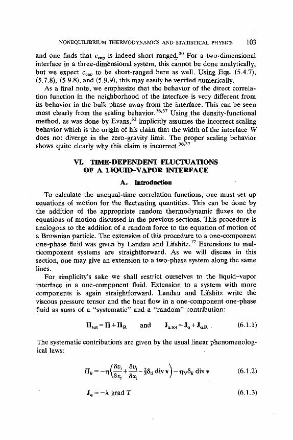
NONEQUILIBRIUM THERMODYNAMICS AND STATISTICAL PHYSICS 103
and one finds that c,, is indeed short ranged.30 For a two-dimensional interface in a three-dimensional system, this cannot be done analytically, but we expect c, to be short-ranged here as well. Using Eqs. (5.4.7), (5.7.8), (5.9.8), and (5.9.91, this may easily be verified numerically.
As a final note, we emphasize that the behavior of the direct correla- tion function in the neighborhood of the interface is very different from its behavior in the bulk phase away from the interface. This can be seen most clearly from the scaling Using the density-functional method, as was done by Evans,32 implicitly assumes the incorrect scaling behavior which is the origin of his claim that the width of the interface W does not diverge in the zero-gravity limit. The proper scaling behavior shows quite clearly why this claim is incorrect.36337
VI. TIME-DEPENDENT F”CTUATI0NS OF A LIQUID-VAPOR INTERFACE
A. Introduction
To calculate the unequal-time correlation functions, one must set up equations of motion for the fluctuating quantities. This can be done by the addition of the appropriate random thermodynamic fluxes to the equations of motion discussed in the previous sections. This procedure is analogous to the addition of a random force to the equation of motion of a Brownian particle. The extension of this procedure to a one-component one-phase fluid was given by Landau and Lifshitz.17 Extensions to mul- ticomponent systems are straightforward. As we will discuss in this section, one may give an extension to a two-phase system along the same lines.
For simplicity’s sake we shall restrict ourselves to the liquid-vapor interface in a one-component fluid. Extension to a system with more components is again straightforward. Landau and Lifshitz write the viscous pressure tensor and the heat flow in a one-component one-phase fluid as sums of a “systematic” and a “random” contribution:
II, = n+ IIR and J,,, = J, + J , , (6.1.1)
The systematic contributions are given by the usual linear phenomenolog- ical laws:
(6.1.2)
Jq := -A grad T (6.1.3)
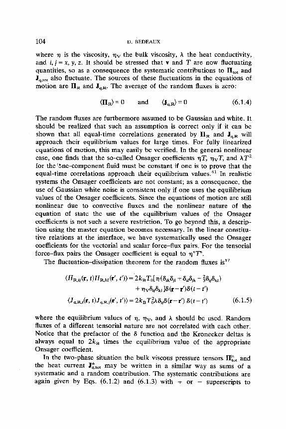
104 D. BEDEAUX
where q is the viscosity, qv the bulk viscosity, A the heat conductivity, and i, j = x, y, z. It should be stressed that v and T are now fluctuating quantities, so as a consequence the systematic contributions to ntot and J,,, also fluctuate. The sources of these fluctuations in the equations of motion are IIR and Jq,R. The average of the random fluxes is zero:
The random fluxes are furthermore assumed to be Gaussian and white. It should be realized that such an assumption is correct only if it can be shown that all equal-time correlations generated by IIR and Jq,R will approach their equilibrium values for large times. For fully linearized equations of motion, this may easily be verified. In the general nonlinear case, one finds that the so-called Onsager coefficients qT, qvT, and AT2 for the ‘Lne-component fluid must be constant if one is to prove that the equal-time correlations approach their equilibrium values?l In realistic systems the Onsager coefficients are not constant; as a consequence, the use of Gaussian white noise is consistent only if one uses the equilibrium values of the Onsager coefficients. Since the equations of motion are still nonlinear due to convective fluxes and the nonlinear nature of the equation of state the use of the equilibrium values of the Onsager coefficients is not such a severe restriction. To go beyond this, a descrip- tion using the master equation becomes necessary. In the linear constitu- tive relations at the interface, we have systematically used the Onsager coefficients for the vectorial and scalar force-flux pairs. For the tensorial force-flux pairs the Onsager coefficient is equal to q T .
The fluctuation-dissipation theorem for the random fluxes is17
where the equilibrium values of q, qv, and A should be used. Random fluxes of a different tensorial nature are not correlated with each other. Notice that the prefactor of the S function and the Kronecker deltas is always equal to 2kB times the equilibrium value of the appropriate Onsager coefficient.
and the heat current JZtot may be written in a similar way as sums of a systematic and a random contribution. The systematic contributions are again given by Eqs. (6.1.2) and (6.1.3) with + or - superscripts to
In the two-phase situation the bulk viscous pressure tensors
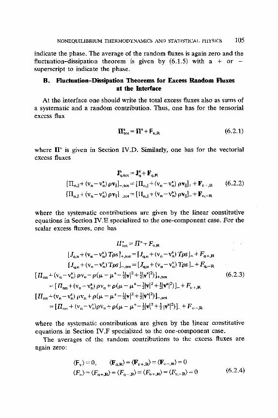
NONEQUILIBRIUM THERMODYNAMICS AND STATISTICAL PHYSICS 105
indicate the phase. The average of the random fluxes is again zero and the fluctuation-dissipation theorem is given by (6.1.5) with a + or - superscript to indicate the phase.
B. Huctuation-Dissipation Theorems for Excess Random Fluxes at the Interface
At the interface one should write the total excess fluxes also as sums of a systematic and a random contribution. Thus, one has for the tensorial excess flux
II:ot = IIs + Fu,R (6.2.1)
where nS is given in Section 1V.D. Similarly, one has for the vectorial excess fluxes
where the systematic contributions are given by the linear constitutive equations in Section N.E specialized to the one-component case. For the scalar excess fluxes, one has
where the systematic contributions are given by the linear constitutive equations in Section 1V.F specialized to the one-component case.
The averages of the random contributions to the excess fluxes are again zero:
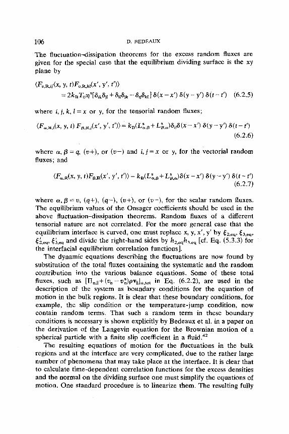
106 D. BEDEAUX
The fluctuation-dissipation theorems for the excess random fluxes are given for the special case that the equilibrium dividing surface is the xy plane by
(Fv,R,ij(X, Y, t)Fv,R,kl(X’? Y’, t‘)>
= 2k~T0V‘[6ik6jr + 6i& - 6y&] 6(X - X’) 6 ( y - y‘) 6(t - t’) (6.2.5)
where i, j , k, 1 = x or y, for the tensorial random fluxes;
where a, p = q, (u+), or (u-) and i, j = x or y, for the vectorial random fluxes; and
where a, p = u, (q+), (q-), (u+), or (u-), for the scalar random fluxes. The equilibrium values of the Onsager coefficients should be used in the above fluctuation-dissipation theorems. Random fluxes of a different tensorial nature are not correlated. For the more general case that the equilibrium interface is curved, one must replace x, y, XI, y’ by t&,, t3,-,
and divide the right-hand sides by h2,eqh3,eq [cf. Eq. (5.3.3) for the interfacial equilibrium correlation functions].
The dynamic equations describing the fluctuations are now found by substitution of the total fluxes containing the systematic and the random contribution into the various balance equations. Some of these total fluxes, such as [11,,11+ (u, - - u ~ ) p ~ , , ] * , ~ ~ ~ in Eq. (6.2.2), are used in the description of the system as boundary conditions for the equation of motion in the bulk regions. It is clear that these boundary conditions, for example, the slip condition or the temperature-jump condition, now contain random terms. That such a random term in these boundary conditions is necessary is shown explicitly by Bedeaux et al. in a paper on the derivation of the Langevin equation for the Brownian motion of a spherical particle with a finite slip coefficient in a
The resulting equations of motion for the fluctuations in the bulk regions and at the interface are very complicated, due to the rather large number of phenomena that may take place at the interface. It is clear that to calculate time-dependent correlation functions for the excess densities and the normal on the dividing surface one must simplify the equations of motion. One standard procedure is to linearize them. The resulting fully
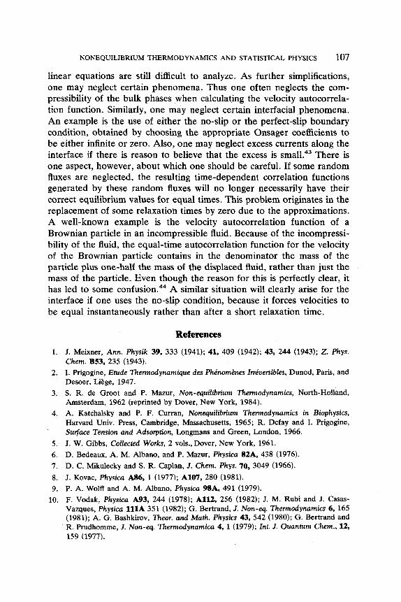
NONEQUILIBRIUM THERMODYNAMICS AND STATISTICAL PHYSICS 107
linear equations are still difficult to analyze. As further simplifications, one may neglect certain phenomena. Thus one often neglects the com- pressibility of the bulk phases when calculating the velocity autocorrela- tion function. Similarly, one may neglect certain interfacial phenomena. An example is the use of either the no-slip or the perfect-slip boundary condition, obtained by choosing the appropriate Onsager coefficients to be either infinite or zero. Also, one may neglect excess currents along the interface if there is reason to believe that the excess is There is one aspect, however, about which one should be careful. If some random fluxes are neglected, the resulting time-dependent correlation functions generated by these random fluxes will no longer necessarily have their correct equilibrium values for equal times. This problem originates in the replacement of some relaxatioh times by zero due to the approximations. A well-known example is the velocity autocorrelation function of a Brownian particle in an incompressible fluid. Because of the incompressi- bility of the fluid, the equal-time autocorrelation function for the velocity of the Brownian particle contains in the denominator the mass of the particle plus one-half the mass of the displaced fluid, rather than just the mass of the particle. Even though the reason for this is perfectly clear, it has led to some confusion.& A similar situation will clearly arise for the interface if one uses the no-slip condition, because it forces velocities to be equal instantaneously rather than after a short relaxation time.
1.
2.
3.
4.
5. 6. 7.
8. 9.
10.
References
J. Meixner, Ann. Physik 39, 333 (1941); 41, 409 (1942); 43, 244 (1943); Z . Phys. Chem. B53, 235 (11943). I. Prigogine, Etude Thermodynamique des Phtnomtnes Irrtversibles, Dunod, Paris, and Desoer, LiBge, 1947. S. R. de Groot and P. Mazur, Non-equilibrium Thermodynamics, North-Holland, Amsterdam, 1962 (reprinted by Dover, New York, 1984). A. Katchalsky and P. F. Curran, Nonequilibrium Thermodynamics in Biophysics, Harvard Univ. Press, Cambridge, Massachusetts, 1965; R. Defay and I. Prigogine, Surface Tension and Adsorption, Longmans and Green, London, 1966. J. W. Gibbs, Collected Works, 2 vols., Dover, New York, 1961. D. Bedeaux, A. M. Albano, and P. Mazur, Physica 8 2 4 438 (1976). D. C. Mikulecky and S . R. Caplan, J. Chem. Phys. 70, 3049 (1966). J. Kovac, Physica A86, 1 (1977); A107, 280 (1981). P. A. Wolff and A. M. Albano, Physica 9 8 4 491 (1979). F. Vodak, Physica A93, 244 (1978); A112, 256 (1982); J. M. Rubi and J. Casas- Vazques, Physica l l l A 351 (1982); G. Bertrand, J. Non-eq. Thermodynamics 6,165 (1981); A. G. Bashkirov, Theor. and Math. Physics 43, 542 (1980); G. Bertrand and R. Prudhomme, J. Non-eq. Thermodynamica 4, 1 (1979); Int. J. Quantum Chem., 12, 159 (1977).
108 D. BEDEAUX
11. B. J. A. Zielinska and D. Bedeaux, Physica 112A, 265 (1982).
12. F. P. Buff, R. A. Lovett, and F. H. Stillinger, Phys. Rev. Lett. 15, 621 (1965).
13. D. Bedeaux and J. D. Weeks, J. Chem. Phys. 82,972 (1985). 14. For this subject and further references, see: J. S. Rowlinson and B. Widon, Molecular
Theory of Capillarity, Clarendon, Oxford, 1982; S. Ono and S. Kondo, in Encyclopedia of Physics, Vol. 10, S. Fliigge, Ed., Springer-Verlag, Berlin, 1960, p. 134; M. S. John, J. S. Dahler, and R. C. Desai, Adu. Chem. Phys. 46,279 (1981); R. Evans, Adu. Phys. 28, 143 (1979); J. K. Percus, in Studies on Statistical Mechanics, Vol. VIII, E. W. Montroll and J. L. Lebowitz, Eds., North-Holland, Amsterdam, 1982, p. 31.
P. M. Morse and H. Feshbach, Methods of Theoretical Physics, Vol. I, McGraw-Hill, New York, 1953.
16. C, Truesdell and R. Toupin, Encyclopedia of Physics, Vol. 111/3, S. Fliigge, Ed., Springer-Verlag, Berlin, 1960.
17. L. D. Landau and E. M. Lifshitz, Fluid Mechanics, Pergamon, Oxford, 1959.
18. A. M. Albano, D. Bedeaux, and J. Vlieger, Physica 99A, 293 (1979).
19. A. M. Albano, D. Bedeaux, and J. Vlieger, Physica 102A, 105 (1980).
20. E. Kroger and E. Kretschmann, 2. Phys. 237, 1 (1970).
21. L. Waldmann, Z. Naturforsch. 22a, 1269 (1967). 22. V. G. Levich, Physicochemical Hydrodynamics, Prentice-Hall, Englewood Cliffs, New
Jersey, 1962.
23. D. Bedeaux and I. Oppenheim, Physica 90A, 39 (1978).
24. L. A. Turski and J. S. Langer, Phys. Rev. A22, 2189 (1980).
25. J. D. Gunton, M. San Miguel, and P. S. Sahni, “The Dynamics of First-Order Phase Transitions,” in Phase Transitions and Critical Phenomena, Vol. 8, C. Domb and J. L. Lebowitz, Eds., Academic, New York, 1983; J. S. Langer, Rev. Mod. Phys. 52, 1 (1980).
26. W. W. Mullins and R. F. Sekerka, 1. Appf. Phys. 34,323 (1963); 35,444 (1964); R. F. Sekerka, “Morphological Stability,” in Crystal Growth: An Introduction, P. Hartman, Ed., North-Holland, Amsterdam, 1973.
27. Ya. B. Zeldovic and Yu. P. Rajzev, Physics of Shockwaues and High Temperature Hydrodynamic Phenomena, Academic, New York, 1966.
28. W. van Saarloos and J. D. Weeks, Physica D12 (Proc. Conf. on Fronts, Interfaces and Patterns), 279 (1984), and references therein.
29. D. Bedeaux and J. D. Weeks, J. Chem. Phys. 82,972 (1985).
30. D. Bedeaux, J. D. Weeks, and B. J. A. Zielinska, Physica 130A, 88 (1985). 31. J. D. Weeks, J. Chem. Phys. 67, 3106 (1977).
32. R. Evans, Mol. Phys. 42, 1169 (1981). 33. D. B. Abraham, Phys. Rev. Lett. 47, 545 (1981).
34. D. Sullivan, Phys. Rev. A25, 1669 (1982).
35. J. D. Weeks, D. Bedeaux, and B. J. A. Zielinska, J. Chem. Phys. 80, 3790 (1984). 36. J. D. Weeks, Phys. Rev. Lett. 52, 2160 (1984).
37. D. Bedeaux, “The Fluid-Fluid Interface,” in Fundamental Problems in Statistical Mechanics VI, E. G. D. Cohen, Ed., North-Holland, Amsterdam, 1985, p. 125.
38. M. C. Wang and G. E. Uhlenbeck, Reu. Mod. Phys. 17, 323 (1945).
15.
NONEQUILIBRIUM THERMODYNAMICS AND STATISTICAL PHYSICS 109
39. M. S. Wertheim, J. Chem. Phys. 65, 2377 (1976). 40. D. G. Triezenberg and R. Zwanzig, Phys. Rev. kit. 28, 1183 (1972). 41. W. van Saarloos, D. Bedeaux, and P. Maxur, Physica A110, 147 (1982); D. Bedeaux,
“Hydrodynamic Fluctuation Theory for a One-Component Fluid in Equilibrium: The Non-Linear Case,’’ in Fundamental Problems in Statistical Mechanics V, E. G. D. Cohen, Ed., North-Holland, Amsterdam, 1980, p. 313.
42. D. Bedeaux, A. M. Albano, and P. Maxur, Physica 88A, 564 (1977). 43. M. Grant and R. C. Desai, Phys. Rev. A27,2577 (1983). 44. See, e.g., D. Bedeaux and P. Mazur, Physica 78,505 (1974), and references therein.