nitrate based high temperature nano-heat-transfer-fluids...

Nitrate based High Temperature Nano-Heat-Transfer-Fluids:

Formulation & Characterisation

Mathieu Lasfargues

Submitted in accordance with the requirements for the degree of

Doctor of Philosophy

The University of Leeds

Institute of Particle Science & Engineering (IPSE)

School of Process, Environmental and Materials Engineering (SPEME)

July, 2014

- ii -

The candidate confirms that the work submitted is his own and that

appropriate credit has been given where reference has been made to the

work of others.

This copy has been supplied on the understanding that it is copyright

material and that no quotation from the thesis may be published without

proper acknowledgement.

© <July, 2014>The University of Leeds <Mathieu Lasfargues>

- iii -

Acknowledgements

I would like to thank my supervisor, Professor Yulong Ding, for giving me the

opportunity to work on such an interesting research project. His constructive

criticisms, inputs, encouragement and supervision have guided me toward

the production of this thesis.

I would also like to express my thanks to the Abengoa Solar New

Technology team particularly Hipolito Lobato Sanchez, Alfonso Rodriguez &

Cristina Prieto for their understanding and patience on this research project

which has seen some highs and lows.

To Hui Cao, Qiao Geng, Christopher Hodges, Salama Omran, Yongliang Li

and Dave Lawlor, thank you for making these four years so interesting. I will

miss our discussions on history, politics and sometimes religion which have

on some occasion turned into heated debates. In many ways, this has

broaden my knowledge and pushed me to be more open-mind.

A big thank you is also in order to Professor Peter J Heggs, for always been

helpful when I approach him.

Finally to my Father, Francis, thanks for teaching me the values of resilience

and hard-work, to my Mother, Marie-Pierre, thanks for the kind words and

encouragement that have carried me through good and bad times, and to

my sister, Anne, thanks for putting up with me.

- iv -

Abstract

This work relates to the development of high temperature heat-transfer-fluid

with enhanced specific heat capacity using nano-particle additives. A

eutectic mixture of nitrate (60 wt% NaNO3 & 40 wt% KNO3) was produced

through ball-milling and characterised on DSC, TGA, Rheometer. The

results obtained showed that the salt mixture melted at 221°C with a heat of

fusion of 97 J/g. Onset of melting was seen at 215°C whilst crystallisation

started at 219°C, reaching a solid state below 217°C with an enthalpy of 97

J/g. Displaying very little overcooling, the salt showed specific heat capacity

of 1.41 J/[°C*g] at 260°C to 1.44 J/[°C*g] at 440°C with viscosity values

changing from 4.8 cP at 250°C to 1.7 cP at 450°C for this Newtonian fluid.

Thermal decomposition of the salt showed that it was stable up to 550°C.

The addition of nano-particles displayed an overall positive effect toward the

specific heat capacity enhancing the latter whilst reducing the onset of

melting due to increased entropy. The addition of 0.1, 0,5 and 1.0 wt%

copper oxide gave the best results with increase of 10.5%, 9,2% and 8,5%

in specific heat capacity respectively. SEM analysis of the samples showed

that the nano-particles clearly disrupted the crystallisation structure showing

a rougher organisation. Rheological tests on 0.1 wt% CuO demonstrated a

slight rise in viscosity due to the addition of nano-particles.

The stability of 0.1 wt% CuO was tested in large scale rigs (>1.0 kg) and

demonstrated that sedimentation of nano-particles did occur. Different

manner of dispersion were tested and revealed that they each affected the

- v -

specific heat capacity differently with some causing negative enhancements

whilst others were positive.

The method of production did not affect the specific heat capacity values,

and current theories point toward the formation of liquid nano-layers as a

reason toward this increase.

- vi -

Table of Contents

Acknowledgements .................................................................................... iii

Abstract ....................................................................................................... iv

Table of Contents ....................................................................................... vi

List of Tables .............................................................................................. ix

List of Figures ............................................................................................. x

Abbreviations ........................................................................................... xix

Chapter 1 Introduction ................................................................................ 1

1.1 Background ................................................................................... 1

1.2 Aims and Objectives ..................................................................... 3

1.3 Layout of Thesis ............................................................................ 3

Chapter 2 Literature Review ....................................................................... 5

2.1 Introduction to the need for Concentrating Solar Power ................ 6

2.2 Concentrating Solar Power Plant .................................................. 7

2.2.1 Line Focusing System: Parabolic Trough & Fresnel Collector ................................................................................ 8

2.2.2 Point Focusing System: Parabolic Dish & Solar Tower ....... 10

2.3 Solar Resources: Direct Normal Irradiance ................................. 12

2.4 Thermal Energy Storage System & CSP Plants .......................... 14

2.5 Types of Thermal Energy Storage Systems ................................ 15

2.6 Form of Thermal Energy Storage ................................................ 21

2.6.1 Thermo-Chemical Heat Storage .......................................... 22

2.6.2 Latent Heat Storage ............................................................ 24

2.6.3 Sensible Energy Storage .................................................... 28

2.7 Heat Transfer Fluids and Thermal Storage Materials for CSP Applications ................................................................................. 29

2.8 Enhancing Thermal Properties of Non-Ionic Fluids with Nano-Particles ............................................................................. 31

2.8.1 Heat Conductivity ................................................................ 31

2.8.2 Specific Heat Capacity ........................................................ 33

2.9 Enhancing Thermal Properties of Ionic Fluids Using Nano-Particles ...................................................................................... 36

2.10 Summary ..................................................................................... 40

Chapter 3 Materials & Methodologies ..................................................... 41

3.1 Preliminary Experimental Results ............................................... 42

- vii -

3.2 Materials: Inorganic Salt & Nano-Particles .................................. 46

3.3 Sample Production ...................................................................... 48

3.3.1 Powder Mixing ..................................................................... 48

3.3.2 Liquid Process ..................................................................... 51

3.4 Experimental Procedures ............................................................ 51

3.4.1 Differential Scanning Calorimeter: Principles & Methodology........................................................................ 52

3.4.1.1 Introduction to DSC ............................................... 52

3.4.1.2 Heat Flow & Enthalpy Measurement ..................... 53

3.4.1.3 Specific Heat Capacity Measurements ................. 54

3.4.1.4 Calibration of DSC ................................................ 58

3.4.1.5 Heat-Flux DSC ...................................................... 60

3.4.1.6 Sample Preparation .............................................. 62

3.4.1.7 Crucible Type: Aluminium ..................................... 62

3.4.1.8 Crucible Type: Stainless Steel .............................. 64

3.4.1.9 Crucible Type: Platinum ........................................ 65

3.4.1.10 Sample Placement & Contact ............................. 67

3.4.1.11 Sample Weighing ................................................ 69

3.4.1.12 Thermal Cycles for DSC ..................................... 70

3.4.2 Thermo-gravimetric Analyser: Principles & Methodology .... 72

3.4.2.1 Introduction to TGA ............................................... 72

3.4.2.2 Balance and Heat Flow Calibration ....................... 73

3.4.2.3 Crucible Type and Sample Preparation ................ 74

3.4.3 Scanning Electron Microscopy ............................................ 75

3.4.4 Rheometer .......................................................................... 76

3.4.4.1 Introduction ........................................................... 76

3.4.4.2 Cone or Flat Plate Setup ....................................... 78

3.4.4.3 Setup .................................................................... 78

3.4.4.4 Calibration Tests : Deionised Water ...................... 81

3.4.4.5 Calibration Tests: Calibration Oil ........................... 82

3.4.4.6 Calibration Tests: Potassium Nitrate ..................... 84

3.4.4.7. Sample Preparation for Rheological Tests ............. 85

Chapter 4 Design and Production of Stability Rigs ................................ 86

4.1 Stability Rigs ............................................................................... 87

4.2 Schematic Design of the 1.6 kg container: .................................. 88

4.3 Schematic Diagram for 1.1 kg container: .................................... 91

- viii -

4.4 Building, Challenges and Alteration ............................................ 92

4.5 Sample Collection ....................................................................... 94

Chapter 5 Results & Discussion: Salt Characterisation without Additives ............................................................................................ 96

5.1 Nitrate Salt Characterisation: ...................................................... 97

5.2 Specific Heat Capacity of Binary Nitrate Salt .............................. 99

5.3 Enthalpy of Change of Binary Nitrate Salt ................................. 102

5.4 Thermo-Gravimetric Analysis of Binary Nitrate Salt .................. 103

5.5 Rheological Analysis of Binary Nitrate Salt ............................... 105

5.6 Summary of Nitrate Salt Characterisation ................................. 107

Chapter 6 Results & Discussion: Salt Characterisation with Additives .......................................................................................... 108

6.1 Zinc Oxide additive (ZnO) ......................................................... 109

6.2 Titanium Dioxide additive (TiO2) ................................................ 111

6.3 Copper additive (Cu) ................................................................. 113

6.4 Silicon dioxide additive (SiO2) ................................................... 115

6.5 Copper Oxide additive (CuO) .................................................... 117

6.6 Summary & Further Discussion ................................................. 119

6.6.1 Summary ........................................................................... 119

6.6.2 Discussion ......................................................................... 122

6.7 Powder vs. Liquid Dispersion .................................................... 126

6.8 Scanning Electron Microscopy Analysis .................................... 129

6.9 Rheological Analysis of 0.1 wt% CuO additives ........................ 134

6.10 Further Discussion & Summary ................................................. 138

Chapter 7 Results & Discussion: Stability Rigs ................................... 140

7.1 Static Rig with Binary Nitrate Salt – No Additives – Negative Control....................................................................................... 141

7.2 Static Rig with Binary Nitrate salt – 0.1 wt% CuO – Positive Control....................................................................................... 144

7.3 Bubbling Rig with Binary Nitrate Salt – 0.1 wt% CuO ................ 146

7.4 Dynamic Rig with Binary Nitrate Salt – 0.1 wt% CuO ................ 148

7.5 Stirring Rig (400 rpm) with Binary Nitrate Salt – 0.1 wt% CuO .. 150

7.6 Further Discussion and Summary ............................................. 152

Chapter 8 Conclusion and Future Work ................................................ 153

List of References ................................................................................... 157

- ix -

List of Tables

Table 1: Degrees of Freedom in Gas ....................................................... 33

Table 2: Percentage difference in Cp between published data compared to HPSS and Pt pans for inorganic carbonate salt mixture without any nano-particles present. .................................. 45

Table 3: Reference materials used by Mettler Toledo for DSC Calibration ......................................................................................... 59

Table 4: TGA/DSC Calibration Metals ...................................................... 73

Table 5: Melting and enthalpy of both salts used in the production of the eutectic mixture ...................................................................... 97

Table 6: Mean percentage enhancement of Cp at 440°C for different type and concentration of nano-particles ...................... 120

Table 7: Onset of Melting ........................................................................ 121

- x -

List of Figures

Figure 1: World Energy Consumption per Year by human in blue compared with estimated renewable and non-renewable resources still available. It can be seen that solar energy outweigh all the other resources by a significant margin [11]. ....... 2

Figure 2: Schematic diagram of CSP [11]. ................................................ 7

Figure 3: Schematic diagram of: a) Parabolic Trough Collector where the receiver tube and the mirrors move in tandem

tracking the sun and b) Fresnel collector display a fixed elevated receiver with a fixed secondary mirror above it to correct the incident light distorted by astigmatism. ........................ 8

Figure 4: Schematic diagram of the absorber tube used in CSP applications. The HTF flows through steel absorber tube [20]. ...... 9

Figure 5: a) Picture of 11 MW PS10 solar tower located in Sanlucar la Mayor, Seville, Spain [18], b) Schematic diagram of Parabolic Dish [25]. ........................................................................... 11

Figure 6: Direct Normal Irradiance of the World. The lighter shade of yellow indicates a higher yearly DNI. .......................................... 12

Figure 7: Left graph shows simulation without thermal storage during cloudy weather, causing fluctuation in solar output (Red) and the use of fossil fuel back-up system (Green) to buffer this. Right graph displays the simulation of the same CSP system but with TES system. No fluctuation in power output (Red) is seen which imply that the backup system not utilized (Green) [33]. .......................................................................... 14

Figure 8: a) Schematic representation of the DSG system [35], b) TES integration in CSP system (Left) [34]....................................... 16

Figure 9: Schematic representation of a thermocline storage system integrated to a CSP Plant [11]. ............................................ 17

Figure 11: Top schematic shows the integration of passive storage to CSP system whilst bottom diagrams display the way in which the materials are put together to create the storage unit........................................................................................ 18

Figure 11: Direct thermal storage [11]. .................................................... 19

Figure 12: Schematic diagram of indirect TES [11]. ............................... 19

Figure 13: Ammonia dissociation used as energy storage[44]. ............ 23

Figure 14: Schematic diagram representing the temperature variation occurring during the melting and crystallisation process. Diagram taken from [58] and edited on paint. ................. 27

Figure 15: Schematic representation of the exposed atoms of a nano-particle which display high surface energy [94]. .................. 38

- xi -

Figure 16: Depiction of the mode of storage in mechanism 2 where the thermal energy would be accumulated at the liquid/solid interface [94]. ................................................................. 38

Figure 17: Graphical representation of liquid layering around nano-particles [94]. ........................................................................... 39

Figure 18: Left picture showed the nano-particle suspension of 1.0 wt % SiO2 in 1 litre of deionised water with a eutectic mixture of carbonate salt (46.6 wt% Li2CO3 + 53.4 wt% K2CO3) dissolved in it. Right picture presented the crystallised carbonate salt where areas of the Petri-dish displayed coarse grain probably caused by faster evaporation rate (red circle) whilst the grain size on the periphery seemed smaller (blue circle). ................................................................................................ 44

Figure 19: Graph displaying the Cp of a binary carbonate salt mixture (46.6 wt% Li2CO3 + 53.4 wt% K2CO3) with and without 1.0 wt% silicone dioxide nano-particles. The black and pink dotted line represent the digitised data from the following paper [13], whilst the red and green squares are results obtained using HPSS pans. The blue and pink triangles were made using of platinum crucibles. .................................................. 45

Figure 20: Top Picture: Different size containers used to produce various amount of salt mixture ranging from a few milligrams to a few kilograms. Bottom-left Picture: Bearing used in the milling process (3 and 9 mm stainless steel, 27 mm ceramic). Bottom-right picture: Milling unit. ................................................... 50

Figure 21: Example of binary nitrate salt doped with copper oxide nano-particles samples produced using the milling process (0.1 wt. % CuO, 0.5 wt. % CuO, 1.0 wt. % CuO and 1.5 wt. % from left to right respectively). In this particular case, a glass jar was used to mix a total amount of 50 grams per batch. 600 grams of 9 mm stainless steel balls were added to grind the powder. .............................................................................................. 50

Figure 22: Graph displaying Heat Flow (mW) against Time (s) for the melting of Indium ........................................................................ 54

Figure 23: Graph displaying the Blank run in Blue, the Sapphire curve in Red (27.737 mg) and the Sample been tested in Black which is also sapphire (27.737). 5 minutes isothermal are used with heating rate of 10°C/min. .......................................... 55

Figure 24: Manually subtracted blank from both sapphires (Black & Red). The orange box represents the dynamic part of the thermal cycle which is used by the software package for specific heat capacity measurements. ............................................ 55

Figure 25: Calculated Cp of Sapphire from 261°C to 444°C. ................. 56

Figure 26: Graph showing the Cp measured using Mettler Toledo Software compared to the calculated values using the raw data. .................................................................................................... 57

- xii -

Figure 27: Indium and Zinc checks confirmed that the instrument was correctly calibrated (In – Hf = -27.88 J/g, Onset = 156.42°C _ Zn – Hf = -107.13 J/g, Onset = 419.44°C). ...................... 59

Figure 28: Schematic diagram of the Mettler Toledo Furnace where S represents the sample and R the reference. .................... 60

Figure 29: Schematic of DSC sensor. Labelled in green (TS& TR) are the areas where the crucibles come into contact with the sensor. The area labelled with the orange arrows is exposed to the chamber. ................................................................................. 61

Figure 30: Damaged sensor due to the contamination of the bottom of the crucible. The red circles represent the areas where the salt has corroded the ceramic surface eventually reaching and damaging the thermocouples embedded below. .... 62

Figure 31: Composite picture of sample production. ............................ 63

Figure 32: Round crimped aluminium crucible on the left prior to tests been carried out whilst on the right is the effect of repeated testing on the shape of the crucible which is distorted (edge is bent). The weight of these aluminium pans is generally located between 49.000 mg to 50.000 mg. .................. 64

Figure 33: 30 µl stainless steel high pressure capsule showing the various parts and how they are assembled (a - c). ........................ 65

Figure 34: Platinum 30 µl pan used for most of the DSC tests. ............ 66

Figure 35: Schematic diagram of pan placement on DSC sensor. The picture on the left portray the perfect positioning of the DSC crucible (orange circle), whereby the flow of heat passes through the pan evenly. The right hand-side picture shows an imperfect placement leading to exposure of some of the sensor (red line) which causes an uneven flow of heat requiring the system to compensate for the irregular thermal flow. .................................................................................................... 67

Figure 36: Contact area between the bottom of the crucibles and the DSC sensor. ................................................................................ 68

Figure 37: Effect of sample placement on heat flow curves for aluminium crucible (Positive curves – Blank, Negative Curves – Sapphire). .......................................................................... 68

Figure 38: Effect of sample placement on heat flow curves for platinum crucible (Positive curves – Blank, Negative Curves – Sapphire)......................................................................................... 69

Figure 39: Ultra-micro-balance set on a granite block and encased in a plastic box to reduce the vibrations coming from the surrounding. ...................................................................................... 70

Figure 40: Thermal cycles used for Cp measurements. ........................ 71

Figure 41: Thermal cycle for enthalpy (J/g) and transition (°C)

tests. ................................................................................................... 71

- xiii -

Figure 42: Schematic diagram of the TGA from Mettler Toledo. ........... 72

Figure 43: Schematic Diagram of SEM .................................................... 75

Figure 44: a) Represents Parallel Plate Model – b & c) Laminar flow of sheared liquid represented by different coloured bands [100]. Two different setups are pictured, cone on plate (b) and plate on plate (c). .................................................................. 76

Figure 47: Graph showing how the shear rate affects the Newtonian and Non-Newtonian behaviour of fluids in relation to both shear stress and viscosity. ................................................. 77

Figure 46: Rheometer setup used to measure viscosity of molten salt. The left picture shows the open two halves of the furnace, with in the middle, either a 65 or 50 mm stainless steel plate onto which the sample is placed with an over-hanging stainless steel cone of 50 mm diameter and 1° angle. The right picture is the setup of the equipment once the furnace is closed. .............................................................................. 79

Figure 47: Schematic diagram of the area of contact between the liquid and the cone & plate setup. Diagram a) has too little fluid between the plate & cone, whilst b) has too much such that the edge of the cone is taken into account (orange circles). Only c) would provide the correct value as only the underside of the cone is utilized for the measurements. .............. 80

Figure 48: Calibration of Rheometer using 0.57 ml of deionised water [101]. The obtained values are significantly accurate (≤ 3.0%) ................................................................................................... 81

Figure 49: Viscosity against shear rate shows that, as expected deionised water behave like a Newtonian liquid [101]. .................. 82

Figure 50: Calibration of Rheometer using Rheotek Calibration Oil 2700-V05 [102]. The obtained values are within 3%. ...................... 83

Figure 51: Viscosity versus shear rate demonstrate the Newtonian character of the calibration fluid used. ........................................... 83

Figure 52: Calibration of Rheometer using KNO3 data from George J. Janz, 1980 published data which shows that the experimental results are within 4.0% of the published data [103]. The following tests were carried out at a constant shear rate of 200 rpm. ....................................................................... 84

Figure 53: The left-hand side represents the dimensions of each of the parts required to produce the tank shown as a 3D sketch on the top-right hand side with the fully build version seen below it...................................................................................... 88

Figure 54: Schematic diagram of the top-plate....................................... 89

Figure 55: Left: Dimension of the impeller blade used. Right: Overhead Stirrer BDC2010 from Caframo utilized in the stirring rig. ......................................................................................... 90

- xiv -

Figure 56: Left: Diagram of the bubbling piece which is centred at the bottom of the tank. Right: Bubbling piece (Red Arrow) connected to 3.0 mm outer diameter tube (Green Arrow) through Swagelok fitting (Orange Line). ......................................... 90

Figure 57: Left: Dimension of each of the three parts soldered together. Top-Right: Dimension of the moving centre-piece providing turbulence in the molten fluid. Bottom-Right: Moving centre-piece in orange is connected to a shaft (blue) which is itself linked to a pneumatic piston providing an up and down motion. ............................................................................. 91

Figure 58: Thermocouples 1 & 2 (Tc 1 & 2 Red box) are attached to wall’s surface of the rig and measure the temperature of the container wall at the bottom (Black Arrow). The orange layer represents the flexible heater band which is in direct contact with the stainless steel wall whilst the blue and green bands are the aluminium foil and the insulating wool respectively. ...................................................................................... 92

Figure 59: Bottom Picture: Heater band damaged through contact with molten salt. Top-left: Newly soldered container. Top-Right: Badly soldered rig with salt leaking through. ..................... 94

Figure 60: Top drawing shows the schematic diagram of the rod which is 200 mm long and 5.8 mm in diameter. The bottom picture displays a collected sample which is roughly 55 mm in length and obtained by dipping the metal rod (red circle) in the container until it touch the bottom. ........................................... 95

Figure 61: Specific heat capacity of each single salt value for both sodium (Red) and potassium (Black) nitrate were measured whilst the theoretical value of the binary mixture (60 wt. % NaNO3& 40 wt. % KNO3) was calculated (Blue). ............................. 98

Figure 62: Specific Heat Capacity of binary combination of nitrate salts (60 wt. % NaNO3 & 40 wt. % KNO3) (Black Square) against results gather from recent literature data [15, 16]. The average specific heat capacity of sapphire (Red Circle) against that of literature value is also showed [109]. .................. 100

Figure 63: Variation of the specific heat capacity of binary nitrate salt (60 wt. % NaNO3& 40 wt. % KNO3) found in the literature [110]. ................................................................................................. 101

Figure 64: Composite diagram showing the specific heat capacity of sapphire reference against measured data with top left drawing displaying the percentage difference between the two [109]. ......................................................................................... 101

Figure 65: Calculated vs. Measured Specific Heat Capacity ............... 102

Figure 66: Melting and crystallisation of binary nitrate salts (60 wt. % NaNO3 & 40 wt. % KNO3). Table within the graph shows the mean value of the 18 tests carried out. ......................................... 103

- xv -

Figure 67: Thermo-gravimetric analysis of binary nitrate mixtures (60 wt. % NaNO3 & 40 wt. % KNO3) where percentage mass loss (left x-axis) and heat flow (right x-axis) are plotted against temperature. ....................................................................... 104

Figure 68: Viscosity measurement with increased temperature of binary nitrate salt mixture (60 wt. % NaNO3 & 40 wt. % KNO3) [116-118]. ......................................................................................... 106

Figure 69: Shear rate plotted against viscosity of the eutectic nitrate salt (60 wt. % NaNO3 & 40 wt. % KNO3) at different temperatures. .................................................................................. 107

Figure 70: Top diagram shows how the addition of various concentrations of ZnO nano-particles to a nitrate blend (60 wt. % NaNO3 & 40 wt. % KNO3) affected the Cp. Bottom left graph is a duplicate of the top but without the error bars, whilst the bottom right display the percentage variation of the mean compared to the salt without additives (cyan). ............ 109

Figure 71: Left hand side diagram showed the variation in melting and crystallisation point with diverse concentration of ZnO nano-particles (0.0 wt%, 0.1 wt%, 0.5 wt%, 1.0 wt% and 1.5 wt%) whilst right hand side diagram demonstrated how the enthalpy of melting or freezing was affected by the nano-additives. ......................................................................................... 110

Figure 72: Top diagram shows how the additions of various concentrations of TiO2 nano-particles to a nitrate blend (60 wt. % NaNO3 & 40 wt. % KNO3) affected the Cp. Bottom left graph is a duplicate of the top but without the error bars, whilst the bottom right display the percentage variation of the mean compared to the salt without additives (cyan). ............ 111

Figure 73: Left hand side diagram showed the variation in melting and crystallisation point with different concentration of TiO2 nano-particles (0.0 wt%, 0.1 wt%, 0.5 wt%, 1.0 wt% and 1.5 wt%) whilst right hand side diagram demonstrated how the enthalpy of melting or freezing was affected by the nano-additives. ......................................................................................... 112

Figure 74: Top diagram shows how the additions of various concentrations of Cu nano-particles to a nitrate mix (60 wt. % NaNO3 & 40 wt. % KNO3) affected the Cp. Bottom left graph is a duplicate of the top but without the error bars, whilst the bottom right display the percentage variation of the mean compared to the salt without additives (cyan). ............................ 113

Figure 75: Left hand side diagram showed the variation in melting and crystallisation point with varied concentration of Cu nano-particles (0.0 wt%, 0.1 wt%, 0.5 wt%, 1.0 wt% and 1.5 wt%) whilst right hand side diagram demonstrated how the enthalpy of melting or freezing was affected by the nano-additives. ......................................................................................... 114

- xvi -

Figure 76: Top diagram shows how the additions of various concentrations of SiO2 nano-particles to a nitrate blend (60 wt. % NaNO3 & 40 wt. % KNO3) affected the Cp. Bottom left graph is a duplicate of the top but without the error bars, whilst the bottom right display the percentage variation of the mean compared to the salt without additives (cyan). ............ 115

Figure 77: Left hand side diagram showed the variation in melting and crystallisation point with varied concentration of SiO2 nano-particles (0.0 wt%, 0.1 wt%, 0.5 wt%, 1.0 wt% and 1.5 wt%) whilst right hand side diagram demonstrated how the enthalpy of melting or freezing was affected by the nano-additives. ......................................................................................... 116

Figure 78: Top diagram shows how the additions of various concentrations of CuO nano-particles to a nitrate mix (60 wt. % NaNO3 & 40 wt. % KNO3) affected the Cp. Bottom left graph is a duplicate of the top but without the error bars, whilst the bottom right display the percentage variation of the mean compared to the salt without additives (cyan). ............................ 117

Figure 79: Left hand side diagram showed the variation in melting and crystallisation point with diverse concentration of CuO nano-particles (0.0 wt%, 0.1 wt%, 0.5 wt%, 1.0 wt% and 1.5 wt%) whilst right hand side diagram demonstrated how the enthalpy of melting or freezing was affected by the nano-additives. ......................................................................................... 118

Figure 80: Illustration of the difference in shape and size of the peaks when nano-particle (1.5 wt% CuO) was present or absent. ............................................................................................. 122

Figure 81: Schematic of heat capacity of Bulk material vs. Nano-particle on the left and on the right a representation of a solid lattice of atoms where the vibrational energy between atoms is responsible for the heat capacity storage. ............................... 123

Figure 82: Schematic diagram of Mode II & III ...................................... 124

Figure 83: Variation in Cp depending on the method used to produce the sample. The bracketed Banerjee name referred to the liquid dispersion whilst the other (Green) was mixed using powder dispersion. ............................................................... 127

Figure 84: Effect of different dispersion method on the melting/crystallisation and enthalpy of change of 1.0 wt% CuO additives compared to binary nitrate salt (60 wt. % NaNO3 & 40 wt. % KNO3) ................................................................. 128

Figure 85: Top-picture: SEM image of non-melted salt crystals containing no additives. Bottom-picture: SEM image of non-melted salt crystal covered with nano-particles (CuO). ............... 129

Figure 86: Scaled up version the bottom picture in Figure 99 (green circle showed the area focused on). ................................. 130

- xvii -

Figure 87: Melted binary nitrate mixture (60 wt. % NaNO3& 40 wt. % KNO3) containing no nano-particle additive. ............................ 131

Figure 88: Melted binary nitrate mixture (60 wt. % NaNO3& 40 wt. % KNO3) containing varied concentration of CuO nano-particle additive (A = 0.1 wt% CuO, B = 0.5 wt% CuO, C = 1.0 wt% CuO & D = 1.5 wt% CuO) ........................................................ 131

Figure 89: Scaled up version the bottom picture in Figure 102 (green circle showed the area focused on). ................................. 132

Figure 90: Scaled up version the bottom picture in Figure 102 (red circle showed the area focused on). ............................................. 132

Figure 91: Viscosity profile of binary nitrate mixture (60 wt. % NaNO3 & 40 wt. % KNO3) containing 0.1 wt% Copper Oxide against increasing shear rate......................................................... 134

Figure 92: Average viscosity taken from 100 - 1000 s-1of binary nitrate mixture (60 wt. % NaNO3 & 40 wt. % KNO3) containing 0.1 wt% Copper Oxide against temperature. ................................ 135

Figure 93: Effect of shear rate on viscosity [126, 127, 129] ................. 136

Figure 94: Difference in specific heat capacity between sample produce in the lab and directly tested on the DSC compared to sample obtained from the rig after different length of time (Standard Deviation <2.0%). ........................................................... 141

Figure 95: Difference in melting point and enthalpy of fusion between sample taken from the rig and salt produced in the lab for binary nitrate mixture containing no additives. ................ 142

Figure 96: Photographs of samples removed from the rigs at different times. ................................................................................ 142

Figure 97: Variation of specific heat capacity of static binary nitrate salt mixture containing 0.1 wt% CuO nano-particles against averages of both static of salt taken from rigs between 0 – 840 hours and salt produced in the lab (Standard Deviation <2.0%). ............................................................................ 144

Figure 98: Melting point and enthalpy of fusion comparison between the presence and absence of CuO with salt taken from the rig and salt made in the lab. ............................................ 145

Figure 99: Photographs of static samples with & without 0.1 wt% CuO removed from the rigs at different times compared to pure binary nitrate salt. Red circle showed accumulation of nano-particles at the tip of the sample. ......................................... 145


- xviii -


Figure 102: Photographs comparing the static sample without additives (Left, 0 hours) to the bubbling rig samples (Right, 0 – 744 hours) removed at different time. ........................................ 147



Figure 105: Photographs comparing the static sample without additives (Left, 0 hours) to the dynamic rig samples (Right, 0 & 168 hours) removed at different time. ........................................ 149



Figure 108: Photographs comparing the static sample without additives (Left, 0 hours) to the stirring (400 rpm) rig samples (Right, 0 – 744 hours) removed at different time. ......................... 151

- xix -

Abbreviations

Cp = Specific Heat Capacity

CSP = Concentrated Solar Power

DNI = Direct Normal Irradiance

DSC = Differential Scanning Calorimeter

DSG = Direct Steam Generation

HTF = Heat-Transfer-Fluid

KNO3 = Potassium Nitrate

NaNO3 = Sodium Nitrate

Solar Salt = Eutectic Binary Mix (60 wt% NaNO3 & 40 wt% KNO3)

SEGS = Solar Energy Generating Station

SEM = Scanning Electron Microscope/Microscopy

TES = Thermal Energy Storage

TGA = Thermo-gravimetric Analyser

- 1 -

Chapter 1 Introduction

1.1 Background

The increased world-wide demand for energy is promoting the research &

development of alternative method of production using renewable sources

(Hydropower, wind farms, photo-voltaics, tidal, CSP) rather than non-

renewable ones (Oil, coal, gas or nuclear) [1-3]. The latter are been utilized

at an increased rate due to the industrial emergence of certain countries

(China, Brazil, India…..) as well as the global rise in population [4]. This is

directly impacting the environment (acid precipitation, ozone depletion and

greenhouse effect) and it is putting pressure on these finite resources which

has led over the last few decades to an increase in fuel prices [5]. Out of all

the renewable energies available, solar energy has the largest potential

(Fig.1), equating about three orders of magnitude that of the world annual

energy consumption [6, 7].

This clean and almost endless source of energy can be transformed into

electricity via two different routes: photovoltaic & concentrated solar power

(CSP). The former technology, which has been widely known and

commercially available for many years, makes use of the short wave region

of solar energy, whilst the latter only utilizes long wave region of the solar

radiation energy.

The research and development of new and more efficient heat transfer fluid

(HTF) is one of the areas which could greatly affect the operation of CSP

- 2 -

plants as the HTF serve a dual purpose of transferring and storing thermal

energy thereby acting as a buffer for power generation [8-10].

Figure 1: World Energy Consumption per Year by human in blue compared with estimated renewable and non-renewable resources still available. It can be seen that solar energy outweigh all the other resources by a significant margin [11].

Currently employed synthetic oil (VP1-Therminol by Solutia Chemistry), is

gradually been replaced with molten salt in CSP plants. Indeed the oil

displays a maximum operating temperature of 400°C, high vapour pressure,

very expensive production costs as well as been environmentally hazardous.

Molten salts on the other hand are cheap, have high operating temperature,

low vapour pressure and are far safer to operate.

However it displays high freezing point and low Cp. Whilst the former can be

solved through heat tracing or altering the ratio and types of salts used, the

latter is more challenging to resolve and will be the basis of this research

[12]. Previous published literatures have shown that the specific heat

capacity of salt mixtures can be altered through the addition of nano-

particles [13-16]. This research will be focused on preparation and screening

- 3 -

of various concentration and types of nano-particles additives to see how

they affect the thermo-physical properties of a binary nitrate mixture of salt

(60 wt. % NaNO3 / 40 wt. % KNO3).

1.2 Aims and Objectives

This work aims to try and understand how the addition of nano-particles will

affect the thermo-physical properties of a eutectic blend of nitrates. The

specific objectives will be as followed:

i. To define the characteristics of a nitrate mixture with the following

composition: 60 wt% NaNO3 + 40 wt% KNO3

ii. To screen a range of nano-particle additives, with concentration

varying from 0.1 wt% to 1.5 wt%

iii. To test if any differences in Cp exist between physical mixing and

dispersion in water followed by evaporation

iv. To characterise the rheology of the selected additive

v. To analyse how nano-particles interact on salt surface before &

after melting of the sample

vi. To investigate how physical dispersion affect the thermal

properties of the blend over time.

1.3 Layout of Thesis

This thesis is composed of 8 Chapters. Chapter 2 provides the reader with a

summary of the relevant literatures regarding the development of renewable

energy and how research within the area of specific heat capacity

- 4 -

enhancement could prove useful both for the renewable energy industries

and for academic understanding.

Chapter 3 describes the materials and methods used in this research. This

include: preliminary data obtained on the DSC, sample production process

for nitrates & carbonates and theories/principles of how the equipments used

function.

Chapter 4 provides details on the dimension of the rigs and how the tests

were conducted.

Chapter 5 presents the results obtained for the analysis of salts without

nano-particles additives.

Chapter 6 looks at the effect of nano-particle additives on the thermo-

physical characteristics of solar salt. It also looks into theoretical aspects

that might explain the underlying physics behind the experimental data

gathered. This chapter will also discuss various variables which might alter

the properties of the doped nano-particle salt blends.

Chapter 7 provides the results of the dispersion rig built to investigate the

effects of physical dispersion on the Cp of salt mixture with and without

additives over time.

Finally Chapter 8 gives a summary of the conclusions obtained in this study

and recommendations of future work to be carried out.

- 5 -

Chapter 2 Literature Review

This chapter contains the relevant literature regarding CSP and its

implementation into the renewable energy field. Sections 2.1-2.3 describe

why solar energy could be a useful alternative to turn to for the production of

electricity, what type of systems are available to achieve this and where can

this technology be implemented around the world. Sections 2.4-2.7 introduce

the reader to the reasons behind the implementation of energy storage

systems, the ways in which thermal energy can be stored and the type of

HTF commonly used. Sections 2.8 & 2.9 relate to non-ionic and ionic nano-

fluid development, how this can be employed for CSP application and the

impact it would have on the technology.

- 6 -

2.1 Introduction to the need for Concentrating Solar Power

Today’s world is driven by energy which is a vital component of the fabric of

our society. Without it, the majority of human activities would cease to

function and the whole world would crumble into pieces, if it was to ever

become unavailable. Given the fact that, the total annual amount of solar

radiation is equal to 2600 times the world annual energy consumption [6],

and that this source of energy is potentially endless, it is not complicated to

see why solar thermal power stations are of great interest in the

development of renewable energy. Furthermore this system of electricity

production releases very little if any gases, fumes or dust in the atmosphere

and would therefore have little or no environmental impact attached to its

operation.

- 7 -

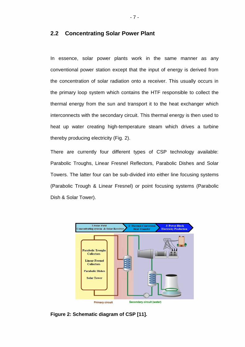
2.2 Concentrating Solar Power Plant

In essence, solar power plants work in the same manner as any

conventional power station except that the input of energy is derived from

the concentration of solar radiation onto a receiver. This usually occurs in

the primary loop system which contains the HTF responsible to collect the

thermal energy from the sun and transport it to the heat exchanger which

interconnects with the secondary circuit. This thermal energy is then used to

heat up water creating high-temperature steam which drives a turbine

thereby producing electricity (Fig. 2).

There are currently four different types of CSP technology available:

Parabolic Troughs, Linear Fresnel Reflectors, Parabolic Dishes and Solar

Towers. The latter four can be sub-divided into either line focusing systems

(Parabolic Trough & Linear Fresnel) or point focusing systems (Parabolic

Dish & Solar Tower).

Figure 2: Schematic diagram of CSP [11].

- 8 -

2.2.1 Line Focusing System: Parabolic Trough & Fresnel

Collector

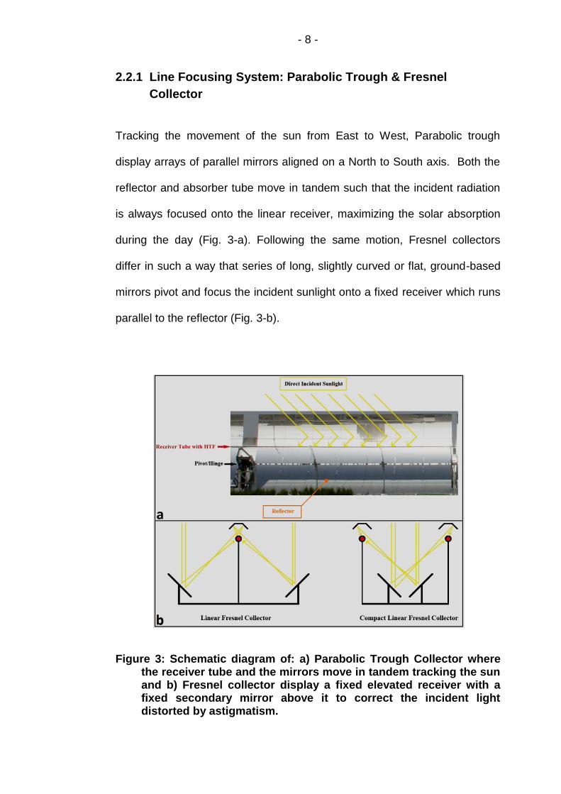
Tracking the movement of the sun from East to West, Parabolic trough

display arrays of parallel mirrors aligned on a North to South axis. Both the

reflector and absorber tube move in tandem such that the incident radiation

is always focused onto the linear receiver, maximizing the solar absorption

during the day (Fig. 3-a). Following the same motion, Fresnel collectors

differ in such a way that series of long, slightly curved or flat, ground-based

mirrors pivot and focus the incident sunlight onto a fixed receiver which runs

parallel to the reflector (Fig. 3-b).

Figure 3: Schematic diagram of: a) Parabolic Trough Collector where the receiver tube and the mirrors move in tandem tracking the sun and b) Fresnel collector display a fixed elevated receiver with a fixed secondary mirror above it to correct the incident light distorted by astigmatism.

- 9 -

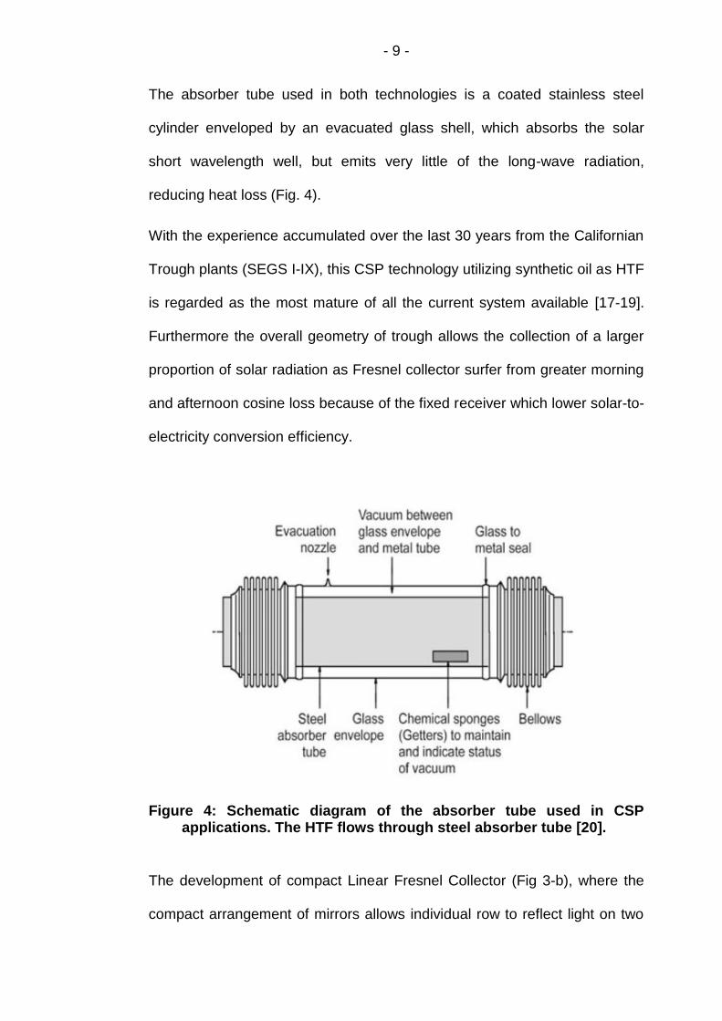
The absorber tube used in both technologies is a coated stainless steel

cylinder enveloped by an evacuated glass shell, which absorbs the solar

short wavelength well, but emits very little of the long-wave radiation,

reducing heat loss (Fig. 4).

With the experience accumulated over the last 30 years from the Californian

Trough plants (SEGS I-IX), this CSP technology utilizing synthetic oil as HTF

is regarded as the most mature of all the current system available [17-19].

Furthermore the overall geometry of trough allows the collection of a larger

proportion of solar radiation as Fresnel collector surfer from greater morning

and afternoon cosine loss because of the fixed receiver which lower solar-to-

electricity conversion efficiency.

Figure 4: Schematic diagram of the absorber tube used in CSP applications. The HTF flows through steel absorber tube [20].

The development of compact Linear Fresnel Collector (Fig 3-b), where the

compact arrangement of mirrors allows individual row to reflect light on two

- 10 -

different linear receivers, could maximise solar collection and minimize

shading and blocking during the operation [21, 22]. Fresnel Collector

development requires cheaper mirrors, less steel and concrete. Furthermore

it displays smaller wind load, greater surface mirror per receptors and a

simpler construction (avoiding the need for rotary joints). However, it still

lacks the accumulated experience of operation and maintenance gathered

by Trough collector over the past few decades. This is reflected by the sheer

number of plants built with 83 world-wide projects, most of which are

commercially producing electricity whilst Fresnel has only 10 working

projects. Leaders in these technologies are Spain and USA.

2.2.2 Point Focusing System: Parabolic Dish & Solar Tower

Using a two axis tracking system (Elevation & Azimuth), this technology

focuses the sun’s radiation onto the receiver with maximal accuracy such

that temperature up to 1000°C can be attained [23, 24]. In parabolic dish

(Fig. 5-b), the sun’s rays are concentrated toward the power conversion unit

(Stirling, micro or Brayton turbine) located at the centre of the parabola. Built

around a light structured frame, this system could potentially operate in

remote location. With research focusing its effort on Stirling engine for power

generation due to its higher solar-to-electricity conversion efficiency, this

technology can offer long-term low maintenance operation [8, 17, 25, 26].

However more research is needed to cut the cost of operation and

maintenance as well as ensure a high level of system reliability.

Solar tower (Fig. 5-a) uses hundreds if not thousands of reflectors called

heliostats which are independently controlled to concentrate the sun’s rays

- 11 -

onto the central receiver located at the top of the tower [27]. This system is

highly flexible in term of design and a variety of heliostats, receivers and

transfer fluids can be used [28]. Currently employed for commercial

production of electricity, power plants are cost efficient and profitable if built

to provide power above 50 MW [29]. Concept of multi-tower solar array are

currently been tested in Australia (Lake Cargelligo) [30].

Figure 5: a) Picture of 11 MW PS10 solar tower located in Sanlucar la Mayor, Seville, Spain [18], b) Schematic diagram of Parabolic Dish [25].

- 12 -

2.3 Solar Resources: Direct Normal Irradiance

CSP technologies rely entirely on DNI which is the fuel of a CSP plant. The

latter is the amount of solar radiation hitting a perpendicular surface tracking

the sun’s movement (pyrheliometer system) and is calculated in kilo-Watts

hour per meter square per year (kWh/m2/year). Thus the design of a CSP

plant is primarily based on this component which can provide an

approximation of the electrical output. It therefore comes as no surprise that

a CSP plant need to be built in a location where the minimum DNI is around

1900 to 2100 kWh/m2/year as any values below that would result in no net

production due constant heat loss through the solar field [8, 17, 18, 27].

Although it might, in the future, be plausible to build CSP plants in lower DNI,

the current estimates (1900 to 2100 kWh/m2/year) are used as standard

throughout the literature. This implies that a cloudy or foggy day will result in

a direct component of zero leading to no electricity production. Hence the

area where a CSP is built is important.

Figure 6: Direct Normal Irradiance of the World. The lighter shade of yellow indicates a higher yearly DNI.

- 13 -

The obtention of a good DNI and reliable clear sky throughout the year lay in

regions between the 15° to 40° in latitude north and south of the equator

where conditions are arid or semi-arid. Regions such as Northern &

Southern Africa, Middle East, Western part of U.S.A, Australia and parts of

South America (Chile, Peru, and Mexico) display the best solar resources for

the installation of such technologies.

The definition of DNI can be based on satellite or ground data. Whilst model

and commercial tools can calculate with good accuracy the solar fraction

available at ground level taking into account atmospheric flux, ground base

measurement provide more accurate data and does not rely on

extrapolation. However, the gathering of such data relies on high quality

measurement devices which most countries within the solar belt lack.

Furthermore if industries or government do have available dataset on a

particular region, they are generally unwilling to share this information with

others [31, 32].

In most cases, the developments of CSP imply extended simulation of the

performance of the plant over several years. In an ideal world, the developer

would have access to dataset of the ground DNI spanning 5 to 10 years

which would give a real estimate of the solar flux from one year to the next.

This would allow to plan and fine tune the simulation accordingly.

Furthermore the localization of the plants needs to be based around the end

users, to meet local energy demands, and has to be optimized and scaled

consequently. This implies developing thermal storage to cope with the

intermittent nature of solar resources.

- 14 -

2.4 Thermal Energy Storage System & CSP Plants

CSP technologies display the advantages of using a form of energy, thermal,

which can easily be coupled to a storage system. The latter is crucial to the

future development and adoption of CSP plants as a general electricity

provider, to solve the intermittency problems encountered by solar

fluctuation. Indeed the DNI varies in intensity during the day and is inexistent

at night.

Figure 7: Left graph shows simulation without thermal storage during cloudy weather, causing fluctuation in solar output (Red) and the use of fossil fuel back-up system (Green) to buffer this. Right graph displays the simulation of the same CSP system but with TES system. No fluctuation in power output (Red) is seen which imply that the backup system not utilized (Green) [33].

This means that production of electricity is only possible during the days if no

energy storage is available. Integrating thermal storage to CSP would allow

the surplus of thermal energy produced to be stored and used during periods

with little or no DNI to drive the generator thereby producing electricity. Such

technology would display several advantageous roles:

- 15 -

Buffering – Any drop in DNI due to transient weather encountered

during the day could be buffered by the storage system. Furthermore

the consumer might not necessarily use the energy when it is

produced. This mismatch between production and utilization would be

solved as the system would store excess energy produced and

release it when needed.

System Stability – Providing enough storage is added to the system,

then the fluctuation in weather would have less impact on the turbine

allowing it to run at a stable rate thereby increasing the overall system

efficiency and probably lifetime of the plant [34].

Increased Annual Capacity Factor – The addition of energy storage

increase the daily usage of the plant as electricity production can be

extended into the night, whereby the TES system takes charge of

production. Therefore the annual capacity factor is increased.

2.5 Types of Thermal Energy Storage Systems

In essence TES systems are very basic and comprise of storage medium,

insulated container and heat exchangers. The design and use of such

technology is in part dictated by the type of material used as well as the way

in which thermal storage is combined to the CSP plants.

Different storage systems will exploit different form of heat storage;

Steam Accumulator (Sensible Heat)

- 16 -

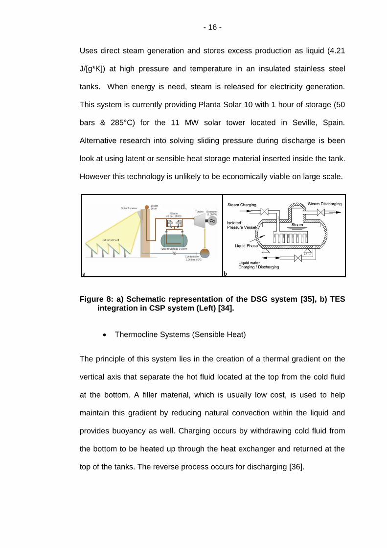
Uses direct steam generation and stores excess production as liquid (4.21

J/[g*K]) at high pressure and temperature in an insulated stainless steel

tanks. When energy is need, steam is released for electricity generation.

This system is currently providing Planta Solar 10 with 1 hour of storage (50

bars & 285°C) for the 11 MW solar tower located in Seville, Spain.

Alternative research into solving sliding pressure during discharge is been

look at using latent or sensible heat storage material inserted inside the tank.

However this technology is unlikely to be economically viable on large scale.

Figure 8: a) Schematic representation of the DSG system [35], b) TES integration in CSP system (Left) [34].

Thermocline Systems (Sensible Heat)

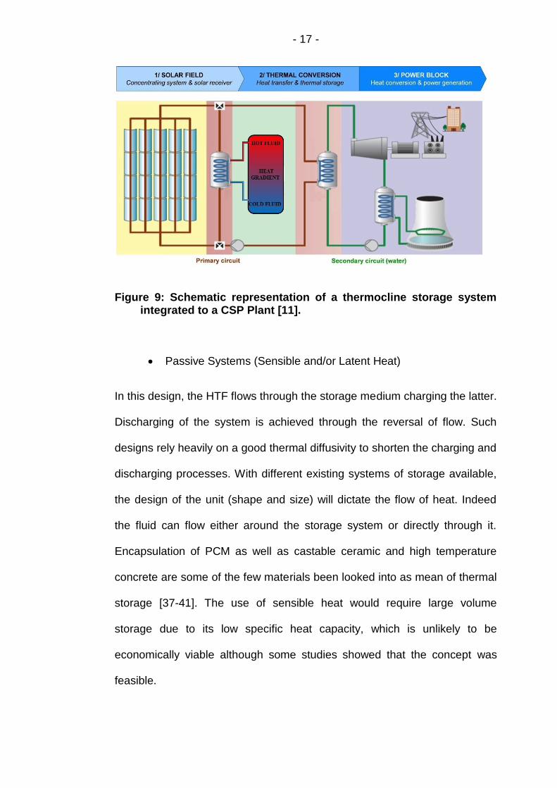
The principle of this system lies in the creation of a thermal gradient on the

vertical axis that separate the hot fluid located at the top from the cold fluid

at the bottom. A filler material, which is usually low cost, is used to help

maintain this gradient by reducing natural convection within the liquid and

provides buoyancy as well. Charging occurs by withdrawing cold fluid from

the bottom to be heated up through the heat exchanger and returned at the

top of the tanks. The reverse process occurs for discharging [36].

- 17 -

Figure 9: Schematic representation of a thermocline storage system integrated to a CSP Plant [11].

Passive Systems (Sensible and/or Latent Heat)

In this design, the HTF flows through the storage medium charging the latter.

Discharging of the system is achieved through the reversal of flow. Such

designs rely heavily on a good thermal diffusivity to shorten the charging and

discharging processes. With different existing systems of storage available,

the design of the unit (shape and size) will dictate the flow of heat. Indeed

the fluid can flow either around the storage system or directly through it.

Encapsulation of PCM as well as castable ceramic and high temperature

concrete are some of the few materials been looked into as mean of thermal

storage [37-41]. The use of sensible heat would require large volume

storage due to its low specific heat capacity, which is unlikely to be

economically viable although some studies showed that the concept was

feasible.

- 18 -

Figure 10: Top schematic shows the integration of passive storage to CSP system whilst bottom diagrams display the way in which the materials are put together to create the storage unit.

Two Tanks Systems (Sensible Heat)

The addition of this system depend on the original design of the plant and

can either be incorporated directly or indirectly:

Direct TES implies that the material flowing and absorbing the solar

radiation is the same as that used in the storage systems. Hence, the

liquid used act as both HTF and TES through the circumvolution of

pipes (Fig. 11).

- 19 -

Indirect TES is where the HTF and TES fluids are different (Fig. 12).

Thus the two loops are interconnected with an extra heat exchanger.

Figure 11: Direct thermal storage [11].

Figure 12: Schematic diagram of indirect TES [11].

- 20 -

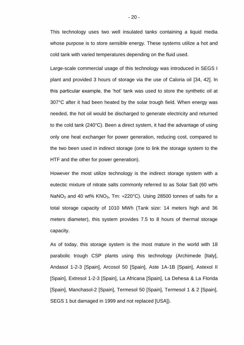
This technology uses two well insulated tanks containing a liquid media

whose purpose is to store sensible energy. These systems utilize a hot and

cold tank with varied temperatures depending on the fluid used.

Large-scale commercial usage of this technology was introduced in SEGS I

plant and provided 3 hours of storage via the use of Caloria oil [34, 42]. In

this particular example, the ‘hot’ tank was used to store the synthetic oil at

307°C after it had been heated by the solar trough field. When energy was

needed, the hot oil would be discharged to generate electricity and returned

to the cold tank (240°C). Been a direct system, it had the advantage of using

only one heat exchanger for power generation, reducing cost, compared to

the two been used in indirect storage (one to link the storage system to the

HTF and the other for power generation).

However the most utilize technology is the indirect storage system with a

eutectic mixture of nitrate salts commonly referred to as Solar Salt (60 wt%

NaNO3 and 40 wt% KNO3, Tm: ≈220°C). Using 28500 tonnes of salts for a

total storage capacity of 1010 MWh (Tank size: 14 meters high and 36

meters diameter), this system provides 7.5 to 8 hours of thermal storage

capacity.

As of today, this storage system is the most mature in the world with 18

parabolic trough CSP plants using this technology (Archimede [Italy],

Andasol 1-2-3 [Spain], Arcosol 50 [Spain], Aste 1A-1B [Spain], Astexol II

[Spain], Extresol 1-2-3 [Spain], La Africana [Spain], La Dehesa & La Florida

[Spain], Manchasol-2 [Spain], Termesol 50 [Spain], Termesol 1 & 2 [Spain],

SEGS 1 but damaged in 1999 and not replaced [USA]).

- 21 -

2.6 Form of Thermal Energy Storage

The design of TES is also dependent on the form of heat used to store

energy which can be: Thermo-Chemical, Latent or Sensible.

Regardless of the form or type of storage employed in the process, there is a

list of desired requirements which the medium should fulfil in order to be of

use [42]:

High Heat capacity (J/g) which is also referred to as energy density.

The higher it is, the smaller the containment unit will be for a given

amount of storage required.

High Thermal conductivity (W/[m2*K]) is extremely important in the

rate of charging and discharging of the unit. This is partly controlled

through the design of the heat exchanger.

Chemical stability implies that the material would not degrade or react

over long period of time.

Mechanical stability of the material refers to its ability to withstand

stress as it is cycled through the heat exchanger at various pressures.

Thermal stability is the operating range of the material. Using a higher

working temperature would result in a higher efficiency.

Compatibility with container material i.e. Corrosive nature of the

medium.

Low environmental impact.

Low cost.

- 22 -

2.6.1 Thermo-Chemical Heat Storage

Based on a reversible reaction, heat is absorbed by an endothermic reaction

leading to the splitting of a compound into separate substances. When heat

needs to be produced, the separate compounds are recombined to give an

exothermic reaction releasing heat.

Potentially, this type of system has the greatest energy density of all of them

as well as the highest efficiency. Indeed breaking molecular bonds require a

large amount of energy, and lead to the production of two separate

substances which can be stored indefinitely and recombined whenever

needed. However the chemical reaction needs to be well understood and

controlled to prevent the creation of undesirable by-products which might

damage the system. Furthermore, if the reaction leads to the production of

gas, then storage become a problem because the units need to be

reinforced and the gas would have to be pumped and therefore pressurized.

This is the case of closed loop system using methane reforming or ammonia

where the products need to be store separately and safely [43, 44].

Methane Reforming:

𝐶𝐻4 + 𝐶𝑂2 + 𝐻𝑒𝑎𝑡 (350°𝐶 − 1000°𝐶) → 2𝐻2 + 2𝐶𝑂

2𝐻2 + 2𝐶𝑂 → 𝐶𝐻4 + 𝐶𝑂2 + 𝐻𝑒𝑎𝑡

Ammonia:

2𝑁𝐻3 + 𝐻𝑒𝑎𝑡 400°𝐶 − 500°𝐶 → 𝑁2 + 3𝐻2

𝑁2 + 3𝐻2 → 𝐻𝑒𝑎𝑡 + 2𝑁𝐻3

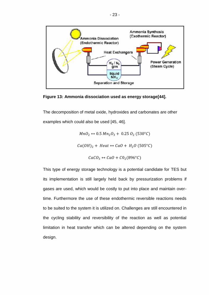
- 23 -

Figure 13: Ammonia dissociation used as energy storage[44].

The decomposition of metal oxide, hydroxides and carbonates are other

examples which could also be used [45, 46].

𝑀𝑛𝑂2 ↔ 0.5 𝑀𝑛2𝑂3 + 0.25 𝑂2 (530°𝐶)

𝐶𝑎(𝑂𝐻)2 + 𝐻𝑒𝑎𝑡 ↔ 𝐶𝑎𝑂 + 𝐻2𝑂 (505°𝐶)

𝐶𝑎𝐶𝑂3 ↔ 𝐶𝑎𝑂 + 𝐶02(896°𝐶)

This type of energy storage technology is a potential candidate for TES but

its implementation is still largely held back by pressurization problems if

gases are used, which would be costly to put into place and maintain over-

time. Furthermore the use of these endothermic reversible reactions needs

to be suited to the system it is utilized on. Challenges are still encountered in

the cycling stability and reversibility of the reaction as well as potential

limitation in heat transfer which can be altered depending on the system

design.

- 24 -

2.6.2 Latent Heat Storage

In latent heat storage, the absorption and release of heat allow the transition

of a material from one phase to the other. The possible transitions are solid-

solid, solid-liquid, solid-gas, liquid-gas and vice-versa. The solid-solid

transition occurs through a structural change as the material accumulates

energy, its molecular arrangement is altered (Amorphous to Crystalline or

the opposite). However this sort of transition only requires a small amount of

energy leading to a limited thermal storage capacity. Solid-gas and liquid-

gas transitions occur with a large volume change and therefore containment

issues often arise as a gas phase is involved, which needs to be

pressurized. Solid-liquid transition is therefore the most favourable option as

this does not suffer from large volume change upon transition and displays a

good energy storage capacity.

Latent heat can be defined by the following equation:

𝑄 = 𝑚 × 𝐿

Q = amount of energy released or absorbed in Joules

m = mass in kg

L = specific latent heat in kJ/kg

Also called phase change material (PCM) or referred to as ‘Heat-of-Fusion

storage’ by A. Abhat 1983, the selection of phase change materials is based

on desirable thermodynamic, kinetic and chemical properties such as [47];

Appropriate phase-transition temperature, which varies with respect

to the system that it is applied to

- 25 -

High specific thermal capacity (kJ/[kg*K]), heat of fusion (J/g), and

density (kg/m3) to lower the size of the thermal unit

High thermal conductivity (W/[m*K]) is important in charging and

discharging phases

Small volume changes upon phase transformation and low pressure

would reduce containment problem of the PCM

Congruent melting, so that phase separation does not take place

Chemical stability of the melts over a long period of time, which

implies reliable changes between solid and liquid form over many

cycles

Low or inexistent super-cooling which hinder the heat extraction

Compatibility with the construction material i.e. not corrosive

They should be resistant to oxidation

Non-toxic

Available and Cheap.

Any chosen PCMs need to fulfil as many of the above conditions as

possible. Because every PCM will have some weaknesses, the development

of a specific storage system will be required, to lower the impact of the latter,

and increase the efficiency of the system [48]. Furthermore the release of

thermal energy from a phase change material is usually an isothermal step

which would offer better quality of heat providing it occurs at a temperature

suited to the system. On CSP application this type of storage technology

would provide a way of maintaining heat production during hours when no

direct sunlight is available. This would allow electricity generation and would

prevent freezing of the HTF within the pipes especially if molten salt are

utilized. Of all the PCMs available, only molten salts seem to fit best toward

- 26 -

the development of such technology. Indeed the availability of a range of salt

whether eutectic or not provides a broad temperature range for its

implementation spanning from low temperature with HITEC (Tm: ≈142°C) (7

wt% NaNO3 – 53 wt% KNO3 – 40 wt% NaNO2) to high temperature with

single salt such as Barium Sulphate (Tm: ≈1680°C) [12]. Been relatively

cheap to purchase and with a low impact on the environment, molten salts

are the best candidates for latent thermal energy storage applications

displaying high latent heat of fusion and relatively low toxicity. However their

corrosive nature and low thermal conductivity need to be addressed through

research. This has been looked at using methods such as encapsulation

(Micro or Macro), impregnation and/or dispersion. Whilst the former method

is more easily applicable to low temperature PCM (<100°C) [49-53],

impregnation [54, 55] and dispersion [56, 57] can be applied to high

temperature.

- 27 -

Figure 14: Schematic diagram representing the temperature variation occurring during the melting and crystallisation process. Diagram taken from [58] and edited on paint.

The use of this technology in CSP application has not yet seen the light of

days, as more research into the storage of PCM and extraction of thermal

energy might be needed. Furthermore development of composite system

(Ceramic/Molten Salt) might provide a way of enhancing the thermal

characteristics of molten salt.

- 28 -

2.6.3 Sensible Energy Storage

It is the ability of a solid, liquid or gas to store energy based on a

temperature difference. The amount of heat stored is directly proportional to

the density, specific heat capacity, and volume as well as temperature

difference such that:

𝑄 = 𝜌 × 𝐶𝑝 × 𝑉 × ∆𝑇

Q = Amount of energy (kJ)

ρ = Density (kg/m3)

Cp = Specific heat capacity (kJ/[kg*K])

V = Volume in (m3)

∆T = Kelvin

This type storage is cheap and can include water, rock, ceramic bricks,

sand, oil, air or any other materials. Each medium displays advantage and

disadvantage such that water has a large thermal capacity, but a low density

compared to rock or ceramic bricks. It is often used as a storage medium in

domestic application such as space heating and to provide warm water at

home or the office [59]. However its operating temperature (20-90°C) makes

it unsuitable for other uses and usual substitutes would be oil or molten salt,

which can function at temperature of up to 400°C for the former, and above

400°C for the latter making them appropriate for use at industrial level or for

thermal solar power station [60, 61]. Both molten salts and oil are used as

heat-transfer-fluids. However, due to their lower price and toxicity, as well as

higher operating temperature, molten salts such as Solar Salts (60%NaNO3-

- 29 -

40%KNO3) are a good alternative. Still one of the disadvantage of using

molten salts is their higher freezing point (≈222°C for Solar Salt) which imply

that heat tracing need to be setup within CSP making use of this technology.

2.7 Heat Transfer Fluids and Thermal Storage Materials for

CSP Applications

There are mainly two types of fluid which can be utilized in CSP applications;

synthetic oil or molten salts. In term of synthetic oil, VP1 is currently the most

utilize type of HTF but the latter displays some disadvantages which is

pushing researchers and industrials to come up with a cheap alternative

material. With an operating range varying between 12°C and 400°C, this

synthetic oil starts to decompose above 400°C creating hydrogen and

various other breakdown products. This is particularly dangerous to the plant

as hydrogen can permeate the stainless steel causing cracks and therefore

leaks to appear within the piping system. This oil is also dangerous to the

environment and will easily pollute the soil which would have detrimental

effect to the surrounding fauna and flora. Furthermore, its high vapour

pressure means that the oil travels through the system as both liquid and

gas phase in a pressurized environment of 25 bars or above. This also

implies that the system has to be topped up with synthetic oil as the

convolution of pipes is not totally hermetic and losses will occur. Finally the

cost of using such material has risen over the years and is now reaching a

significant percent of the total investment cost of the plant. One of the

advantages of this oil is its high specific heat capacity at 400°C which is of

2.628 J/[g*K].

- 30 -

On the other hand, the Cp of molten salt is relatively low compared to VP1

with solar salt displaying a mean value of ≈1.55 J/[g*K]. Furthermore its high

melting point entails heat tracing, such that the system is equipped with back

up heaters to ensure the salt does not freeze within the pipes which would

cause a blockage and would damage the system. However unlike VP1, it is

not toxic and would not penetrate the soil if a leakage were to occur. Instead

the salt would readily crystallize. Providing the system can be safely kept

above crystallization, the maximum operating temperature of this salt is

much greater than that of VP1 with Solar salt capable of handling up to

600°C. As efficiency of CSP plants increases with higher temperature,

inorganic salt are a good alternative to propose. The low vapour pressure of

solar salt also means that the travelling fluid will almost always be in the

liquid phase allowing the system to run with low pressure. Another variable

to take into account is the corrosion of inorganic salt which is highly

dependent on the type of mixture used. Chloride salts are generally very

corrosive whilst carbonate and nitrate salts have a lower corrosive nature

which is why research is focused on the utilization of either nitrate or

carbonate salt as HTF. On top of that, the purchasing price of salt is far

lower than that of VP1 making it attractive to industries and particularly CSP

applications.

However one of the key parameters in HTF is the specific heat capacity of

the material. Indeed, this number relates to the amount of energy the fluid is

capable of storing with an increase in temperature. This will directly affect

the CSP plants providing a decrease in electricity prices as the energy

density of the material is increased. Therefore research into the field of

molten salt nano-fluid is a popular topic which is currently the focus of much

- 31 -

investigation and discussion. Nano-fluid has been a highly researched area

in the last 20 years and discovery of its effects on thermal behaviour of low

temperature fluid has been largely explored. This is not the case for high

temperature materials.

2.8 Enhancing Thermal Properties of Non-Ionic Fluids with

Nano-Particles

2.8.1 Heat Conductivity

Addition of nano-particles into a base liquid forms a two-phase mixture. Such

a mixture (suspension) is termed nano-fluid.

Suspension of minute quantities of nano-particles in liquid solvents was first

coined as ‘nano-fluid’ by Choi in 1995 [62]. With nominal size ranging from

1-100 nm, these nano-particles have been reported to display anomalous

enhancement of the thermal characteristic of the fluid within which they are

suspended. Lee et. Al (1999), reported that the addition of various fraction

(0.1 vol.% to 0.5 vol.%) of Copper Oxide (CuO) and Aluminium oxide (Al2O3)

of 20-40 nm, all increased the thermal conductivity of both ethylene glycol

and water [63]. This was reaffirmed by Das et. Al (2003) who showed a

maximum enhancement of 24.3% with 4.0 vol. % of Al2O3 and 36% with 4.0

vol. % CuO suspended in water [64]. Other base fluids such as pumped oil,

glycerol and toluene have shown enhanced thermal conductivity with the

minute addition (Maximum of 5.0 vol. %) of various nano-particles such as

Al2O3, Au, TiO2, Cu, CuO and Carbon Nano-tube (CNT) [65-72].

- 32 -

The complex nature of nano-fluids has made it difficult to model and

reported data have showed that the size of the particle, concentration,

particle surface properties, interaction between base liquid & particles,

shape of the particles as well as the type of nano-particles utilized could

affect the thermal characteristics in very different manners [64, 69, 73, 74].

The literature is full of papers proving and reporting these atypical

improvements in the thermal conductivity [73], and recent theory &

understanding of the gathered data point toward the effective medium

theory by Maxwell as a good model for the prediction of thermal conductivity

if aggregation of particles is taken into account [75, 76].

Furthermore the stability of a nano-fluid is also affected by the methodology

used to stabilise them. The aim in suspending nano-particles in a fluid is to

prevent their excessive aggregation and sedimentation over time. This can

be achieved via a physical mean which makes use of an ultra-sonicator or

via high-shear rate mixer with the aim of breaking potential agglomerate and

homogenising the fluid [77]. Alternatively chemical stabilizers usually called

dispersants surfactants are added to the mixture to enhance the stability of

the fluid and prevent aggregation. The choice in the latter is highly

dependent on the type of base fluid employed in the process [78].

Furthermore chemical alteration of surface properties of nano-particles (e.g.

SiO2) to enhance stability through the addition of chemically bonded side

chain (e.g. Silane) has also been looked at by Yang et Al. (2010) [79] and

probably others. Finally altering the pH of the solution is one of the ways to

improve the stability of aqueous based nano-fluids [80, 81]. Whilst each of

the method has an impact on the stability of nano-fluids [77, 78, 82], Xuan et

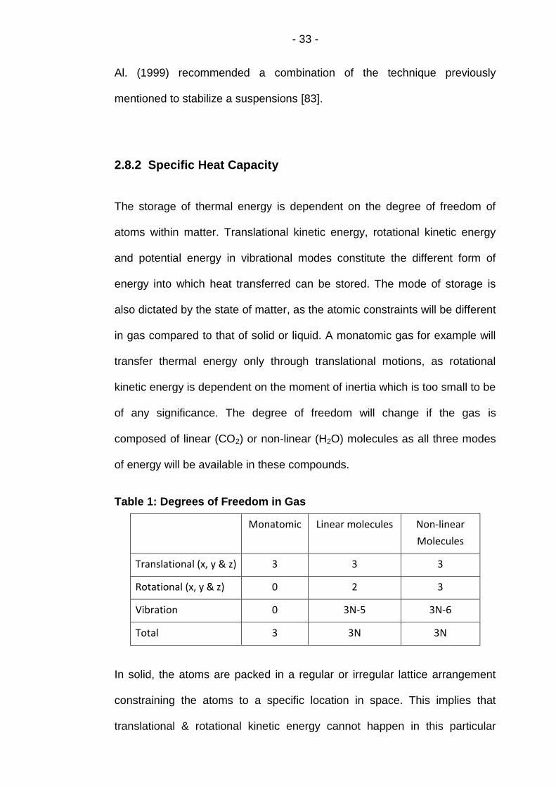
- 33 -

Al. (1999) recommended a combination of the technique previously

mentioned to stabilize a suspensions [83].

2.8.2 Specific Heat Capacity

The storage of thermal energy is dependent on the degree of freedom of

atoms within matter. Translational kinetic energy, rotational kinetic energy

and potential energy in vibrational modes constitute the different form of

energy into which heat transferred can be stored. The mode of storage is

also dictated by the state of matter, as the atomic constraints will be different

in gas compared to that of solid or liquid. A monatomic gas for example will

transfer thermal energy only through translational motions, as rotational

kinetic energy is dependent on the moment of inertia which is too small to be

of any significance. The degree of freedom will change if the gas is

composed of linear (CO2) or non-linear (H2O) molecules as all three modes

of energy will be available in these compounds.

Table 1: Degrees of Freedom in Gas

Monatomic Linear molecules Non-linear

Molecules

Translational (x, y & z) 3 3 3

Rotational (x, y & z) 0 2 3

Vibration 0 3N-5 3N-6

Total 3 3N 3N

In solid, the atoms are packed in a regular or irregular lattice arrangement

constraining the atoms to a specific location in space. This implies that

translational & rotational kinetic energy cannot happen in this particular

- 34 -

state. Thus storage of thermal energy is only attainable through vibrational

mode. The latter is due to connection between atoms which can be

visualized as springs. The amount of oscillation of this lattice (thermal

phonon) is dependent on the temperature and is well described by the

Einstein or Debye theory of heat capacity.

Whilst there is a good theoretical understanding of heat capacity in both

solid and gas, the same cannot be said of liquids. In this state, both

translational and vibrational modes of energy storage take place. Devising a

model for this type of system is difficult as the interactions taking place in

this state are specific to the type of liquid employed. Yakov Frenkel in 1940s

emitted the idea that above a certain frequency, molecule in a liquid could

behave like a solid and therefore support phonon. Due to the increased

mobility of atoms, only frequencies above the relaxation time of liquid

allowed the shear wave to propagate. The model implemented by Bolmatov

et. al 2012 predicted quite accurately the liquid Cp of 21 samples using

Frenkel phonon theory [84].

With the literature agreeing on the positive effect of nano-particles on the

rise of thermal conductivity in non-ionic base fluid, very little research was

carried out on the Cp of such combination [85]. However, one could think of

specific heat capacity as the direct opponent of thermal conductivity. Indeed

measured in W/[m*K], thermal conductivity represents the transfer of energy

whilst Cp (J/[g*K]) is define as storage capacity. If a HTF were to have a

large thermal conductivity, one would think that its capacity to retain heat

would be impaired as any heat stored would be readily given away. This is

usually measured through thermal diffusivity (m2/s) where:

- 35 -

𝛼 = 𝜅

𝜌𝐶𝑝

κ is thermal conductivity (W/[m*K])

ρ is density (kg/m3)

Cp is specific heat capacity (J/[kg*m])

And indeed this seems to be the case in non-ionic fluid where the specific

heat capacity seems to decrease upon the addition of nano-particles and the

increase in thermal conductivity. Measurements done by Zhou et al. 2008

showed that the suspension of Al2O3 nano-particles in water decreased its

Cp with increased volume fraction [85]. This was also used to determine

whether modelling of heat capacity using classical and statistical mechanism

would agree with the obtained data, which it did, with the following equation

[85];

𝐶𝑝 ,𝑛𝑓 = ∅(𝜌𝐶𝑝)𝑛 + (1 − ∅)(𝜌𝐶𝑝)𝑓

∅𝜌𝑛 + (1 − ∅)𝜌𝑓

Where Cp, ∅, ρ, nf, n & f respectively represent specific heat capacity,

volume fraction, density, nano-fluid, nano-particle and fluid. Furthermore

tests carried by Pantzali’s research team showed that the addition of CuO

nano-particles to water also caused a decrease in Cp of 35.4% with the

addition of 8% v/v fraction of nano-particles. Similarly to Zhou et al. 2008, a

decrease in volume fraction of CuO nano-particles cause an increase in Cp

such that 2% v/v of CuO only led to 11% loss in Cp [86]. Both papers [85,

86] argue that the equation from Pak & Cho 1998 [87] for the calculation of

Cp over-estimated its value. This is sustained by Saeedinia et, al. 2012 who

also demonstrated the decrease in Cp of oil when nano-particles of copper

- 36 -

oxide (0.2%, 0.5%, 1.0% & 2.0%) were added [88] and concurred that Pak &

Cho 1998 Cp model over-estimated the results.

It seems that the publications agree on the fact that stable suspension of

nano-particles within a non-ionic fluid leads to a loss of specific heat capacity

which is dependent on the percent present. But report on enhancement of

Cp was observed by Nelson (2007) where the addition of 0.6 weight % of

exfoliated graphite to polyalphaolefin enhanced the specific heat capacity by

50% [89]. The obtention of those results are surprising but could be

explained by the interaction of exfoliated graphite sheets with

polyalphaolefin.

2.9 Enhancing Thermal Properties of Ionic Fluids Using

Nano-Particles

The research into non-ionic nano-fluid has showed us that providing the

nano-powders are well suspended and disperse, there is an increase in the

thermal conductivity and a decrease in specific heat capacity of the fluids.

However research carried out by Shin et al. (2011) on ionic fluid

demonstrated that the addition of 1.0 wt% of silica nano-particles to a binary

mixture of lithium carbonate & potassium carbonate (62:38 ratio) led to a Cp

enhancement of 19-24% in liquid status (525°C - 555°C) compared to the

base salt [90]. With that, it was showed that the size of the nano-particles (5,

10, 30 and 60 nm diameter) did not seem to affect the increase in Cp for

SiO2 [14]. These results are unusual as the specific heat capacity of oxide

nano-particles (≈1.0 J/[g*K]) is lower than that of salts. However experiments

- 37 -

have showed that nano-particles generally display a higher energy structure

than coarse grain due to their high surface area to volume ratio leading a

larger blue shift in infrared spectroscopy [91, 92]. Indeed due to their smaller

size, nano-particles have a greater proportion of exposed atoms and thus an

enhanced surface energy which cannot be neglected. Research by

Tiznobaik et al. 2013 pointed out that the enhancement in Cp might be due

to the formation of nano-structures which can be negated through the

prevention of electrostatic interaction between nano-particles and ions [93].

Indeed the addition of 0.02 wt% of sodium hydroxide to a binary mixture of

carbonates containing 1.0 wt% SiO2 led to similar Cp to that of pure salts

whilst its absence promoted a rise of ~26% [93]. This could imply that

electrostatic forces within ionic fluid might play a role in specific heat

capacity enhancement.

Recent theories points toward three possible mechanisms in the

enhancement of specific heat capacity [94]:

Mechanism 1 relates to the fact that the specific heat capacity of

nano-particles is larger than its bulk value. If one imagine that a

sphere is made up of thousand of atoms, and that the latter are

constrained and held together by spring-like bonds. Then the atoms

on the surface, which are exposed, will have a lower vibrational

energy than those found on the inside of the sphere. Therefore if the

surface area to volume ratio is increase, the amount of ‘exposed’

atoms will drastically rise leading to an increase in specific heat

capacity which would be stored through an increased vibrational

energy of the ‘exposed’ surface atoms of the sphere [91, 95].

- 38 -

Figure 15: Schematic representation of the exposed atoms of a nano-particle which display high surface energy [94].

Mechanism 2 relates the solid-fluid interaction energy, also called

Kapitza resistance, which occurs during the transfer of heat between

the fluid phase (base liquid) and the solid phase (nano-particles). This

thermal resistance could be considered negligible on macro-scale, but

nano-scale displays a large surface area to volume ratio increasing

the effective specific heat capacity. This thermal resistance would act

as a storage unit holding the energy within this boundary [96, 97].

Figure 16: Depiction of the mode of storage in mechanism 2 where the thermal energy would be accumulated at the liquid/solid interface [94].

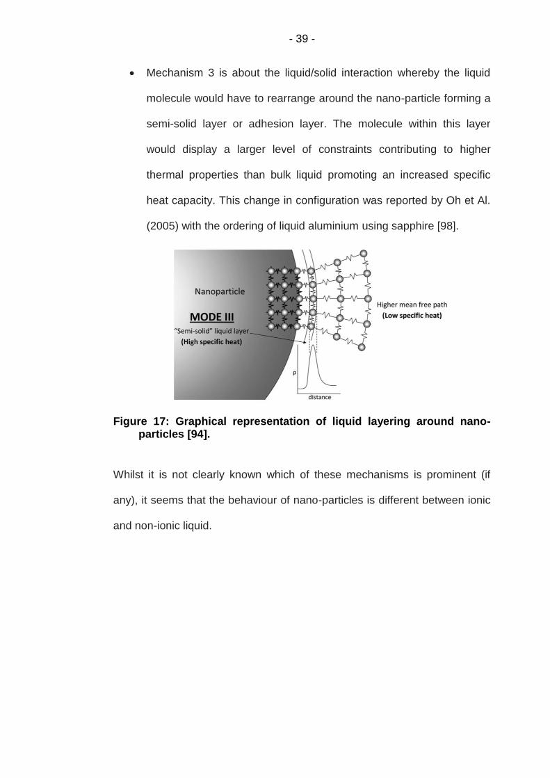
- 39 -

Mechanism 3 is about the liquid/solid interaction whereby the liquid

molecule would have to rearrange around the nano-particle forming a

semi-solid layer or adhesion layer. The molecule within this layer

would display a larger level of constraints contributing to higher

thermal properties than bulk liquid promoting an increased specific

heat capacity. This change in configuration was reported by Oh et Al.

(2005) with the ordering of liquid aluminium using sapphire [98].

Figure 17: Graphical representation of liquid layering around nano-particles [94].

Whilst it is not clearly known which of these mechanisms is prominent (if

any), it seems that the behaviour of nano-particles is different between ionic

and non-ionic liquid.

- 40 -

2.10 Summary

This chapter’s aim was to summarise the relevant literature surrounding

renewable energy technologies, and how the research and development,

within the area of specific heat capacity enhancement of HTF could

positively affect the implementation of CSP around the world. However, a

vast gap in the literature can be seen when it comes to specific heat capacity

measurements, with most of the papers published concentrating on the use

of carbonate salts. Very little has been done on nitrate salts.

Furthermore the basic characteristics of the salt mixtures are difficult to

locate, and no study has concentrated its effort on defining these. Providing

that any enhancements in a material is determined by its baseline, it is

crucial to ensure the results of pure inorganic salt mixture are within an

acceptable range before any other experiments are conducted.

This PhD thesis will therefore concentrate on defining the basic

characteristic of solar salt and investigate the effect of various nano-particles

on the thermo-physical characteristics of the salt with particular attention

paid to specific heat capacity measurements.

- 41 -

Chapter 3 Materials & Methodologies

This chapter starts with a description of preliminary results attained which

provided vital information for future design of the experiments. This is

followed by a description of the materials used as well as the procedure

employed to produce the samples. The chapter is terminated by a

description of the equipments used for characterisation of the salts as well

as an explanation of how they operated and the way in which they were

calibrated for the purpose of the tests.

- 42 -

3.1 Preliminary Experimental Results

The initial first step taken in this research was to try and validate published

data by mimicking the methodology of Banerjee’s 2010 research which was

concentrated on the enhancement of specific heat capacity in binary

carbonate salt using 1.0 wt% silicon dioxide [13]. The reason behind the

choice of this particular paper was the obviously large enhancement seen in

the specific heat capacity which could then be tried on nitrate salts. If the

methodology was successful, the aim was to test it on nitrate salt with a

variety of different nano-particles. Following the paper’s protocol (ratio), 4.59

grams of Li2CO3 and 5.26 grams of K2CO3 were dissolved in 1 litre of

deionised water. Then 0.15 grams of silicon dioxide nano-particles were

added and dispersed through sonication for a couple of hours until a

transparent milky solution was obtained (Fig. 18). In the same manner, a

control exempt of nanoparticles was produced (4.66 grams of Li2CO3 + 5.34

grams of K2CO3 in 1 litre). The dispersion of nano-particles seemed stable

over the next few days with aggregation only starting to appear after a few

weeks without sonication. The aggregates were then easily broken apart

through another round of sonication and re-dispersion of the nano-particles

was easily achieved. The following step was to evaporate (on a hot-plate at

60°C using Petri-dished) and fully dry the crystallised mixtures at

temperature above 150°C to remove any water molecules bound to the salt

forming hydrates. Ensuring that the salt was fully dried was extremely

important so as to prevent the hermetically sealed capsule from blowing up

due to the pressure build up from the vaporization of water molecules.

- 43 -

The crystallised salt obtained (Fig. 18) showed that the rate of evaporation of

water was not homogenous and some areas displayed much finer grain size

than others. The salt crystals were removed using a clean razor blade and

both coarse and fine grains were mixed together and tested.

Whilst the methodology for producing the salt was similar to what was

written in Banerjee’s 2010 paper [13], the actual DSC equipment differed.

Therefore the thermal cycle was altered. When using High Pressure

Stainless Steel (HPSS) 30 µl pan, the following cycle was used:

Isothermal ramp of 5 minutes at 530°C

Dynamic ramp from 530°C to 560°C at 10°C/min


However when platinum pan (30 µl) were utilised a slightly different cycle

was employed:


Dynamic ramp from 520°C to 560°C at 10°C/min


There were no particular reasons behind this slight change of thermal cycle

aside from the fact that more data could be gathered. The obtained results

were very interesting as the variation was extremely different depending on

the type of pans used when nano-particles were present. However little

variation was seen when pure carbonate salt was tested.

Indeed when using HPSS pans (Fig. 19 red and green square), the data was

similar to that of the paper [13] (Fig. 19 pink and black dotted line) as

showed below with enhancement of around 100% seen when nano-particles

- 44 -

were added, although the standard deviation in data was relatively high with

a maximum of ±6.7%.

Figure 18: Left picture showed the nano-particle suspension of 1.0 wt % SiO2 in 1 litre of deionised water with a eutectic mixture of carbonate salt (46.6 wt% Li2CO3 + 53.4 wt% K2CO3) dissolved in it. Right picture presented the crystallised carbonate salt where areas of the Petri-dish displayed coarse grain probably caused by faster evaporation rate (red circle) whilst the grain size on the periphery seemed smaller (blue circle).

Using platinum crucibles painted a totally different picture in term of the

results gathered as a small decrease in Cp (≈ -1.77%) was seen when nano-

particles were utilized. But the results for the pure carbonate salt were

similar regardless of the type of pan used (Table. 2). This was not the case

when nano-particles were involved as the difference between HPSS pan and

Pt pans is around 100% which raised the question as to where did the

difference came from?

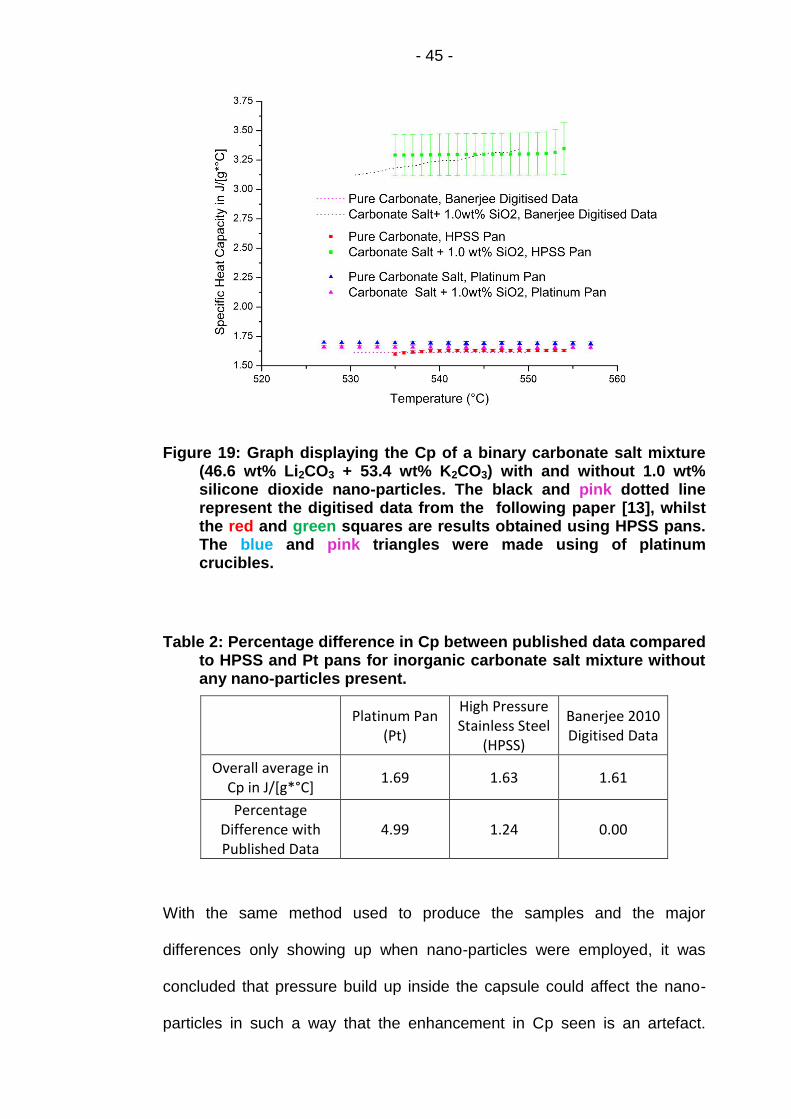
- 45 -

Figure 19: Graph displaying the Cp of a binary carbonate salt mixture (46.6 wt% Li2CO3 + 53.4 wt% K2CO3) with and without 1.0 wt% silicone dioxide nano-particles. The black and pink dotted line represent the digitised data from the following paper [13], whilst the red and green squares are results obtained using HPSS pans. The blue and pink triangles were made using of platinum crucibles.

Table 2: Percentage difference in Cp between published data compared to HPSS and Pt pans for inorganic carbonate salt mixture without any nano-particles present.

Platinum Pan

(Pt)

High Pressure Stainless Steel

(HPSS)

Banerjee 2010 Digitised Data

Overall average in Cp in J/[g*°C]

1.69 1.63 1.61

Percentage Difference with Published Data

4.99 1.24 0.00

With the same method used to produce the samples and the major

differences only showing up when nano-particles were employed, it was

concluded that pressure build up inside the capsule could affect the nano-

particles in such a way that the enhancement in Cp seen is an artefact.

- 46 -

These tests revealed the challenging nature of measuring specific heat

capacity particularly with corrosive material such as inorganic salts.

Furthermore it also questioned the published data and the actual procedure

used to produce the salt mixture. With this in mind, the processes of salt

production, characterisation and testing were re-design to encompass all the

challenges previously encountered when working with carbonate salts.

3.2 Materials: Inorganic Salt & Nano-Particles

The main components used in the development of eutectic salts were either

nitrate or carbonate based compound. Purchased in anhydrous forms with

varying grains size and shape depending on the manufacturer, the powders

were generally grinded using different processes which will be described

later on.

Regarding, the carbonate mixture mentioned above, the following salts and

ratio were used: anhydrous lithium carbonate (99.0 % Pure) (46.6 wt.%)

(MERCK) and potassium carbonate (99.0 % Pure) (53.4 wt.%) (FISHER

BIOREAGENT).

The binary nitrate mixture was composed of anhydrous sodium nitrate

(FISHER) (98% Pure) (60 wt. %) and potassium nitrate (SIGMA-ALDRICH)

(98% Pure) (40 wt. %), this ratio of salt was the basis for all the subsequent

tests carried out.

- 47 -

The other components present in some of the mixtures were nano-particles

with percentage weight ratio varying from 0.1 to 1.5. The specifications of

the nano-particles were taken from the manufacturer sites:

Copper Oxide (CuO):

Producer: Nanophase Technologies Corporation

Purity: 99.0+%

APS: 29 nm (determined from SSA)

SSA: 32 m2/g (BET)

Appearance: Black powder

True Density: 6.5 g/cc

Morphology: Equi-axed and nearly spherical

Crystal Phase: Monoclinic

Titanium Oxide (TiO):

Producer: NanophaseNanoTek

Purity: 99.5+%

APS: 34 nm (determined from SSA)

SSA: 45 m2/g (BET)

Bulk density: 0.25 g/cc

True density: 3.95 g/cc

Morphology is nearly spherical

Crystal phase: 80% anatase and 20% rutile

Zinc Oxide (ZnO):

Producer: Nano-structured and Amorphous materials

Purity: >99%

Bulk Density: 0.30-0.45 g/cm3

APS: 40 nm

SSA: 50-70 m2/g

- 48 -

Silicon Dioxide (SiO2):

Producer: Sigma Aldrich

Assay: 99.5% trace metals basis

Form: Spherical, porous

Particle size: 5-15 nm (TEM)

Surface area: 590-690 m2/g (TEM)

Bp: 2230 °C (lit.)

Mp: >1600 °C (lit.)

Density: 2.2-2.6 g/ml at 25 °C

Bulk density: 0.068 g/ml

Copper (Cu):

Producer: US Research Nanomaterials

Cu purity: >99%

Form: Spherical APS: 70 nm SSA: 6-8 m2/g

3.3 Sample Production

The production of eutectic salt can be done either by physically mixing the

different powders together with the aim of attaining a homogenous mixture

or by taking advantage of the solubility of salts into water.

3.3.1 Powder Mixing

The inorganic salts were weighed and mixed together following the ratios

mentioned above (Section 3.2). Then the powdered mixtures were inserted

into clean glassware. The latter had been sonicated with purified water and

- 49 -

surfactant as well as dried in an oven at 80°C before been used. Stainless

steel (3 or 9 mm diameters) or ceramic (27 mm diameter) ball bearings were

added inside glass or ceramic jar and the latter was placed onto a mill to

physically crush and mix the samples (Fig. 20). The ball bearings were

sonicated in purified water as well as acetone before been dried in the oven

at 80°C prior to their utilization. This step was to ensure the cleanliness of

the bearings and remove any rust particles on their surface to lower

contamination of the salt. The type of bearing or container used depended

entirely on the amount that needed to be produced. Low quantities could be

created using a pestle and mortar whilst larger amounts will have required

the use of vessel with the correct proportion.

The milling process (80-100 rpm) was checked every half-hour to monitor

the consistency of the powders and ensure that it was not sticking to the side

of the wall. Once flour like consistency was attained which roughly equated

to a grain size ranging from 1 µm to 100 µm, the process was stopped. This

took around 2 to 3 hours.

After obtaining a homogenous binary mixture, different types of nano-

particles were introduced in the eutectic salt with the following ratio: 0.1 wt%,

0.5 wt%, 1.0 wt% and 1.5 wt%. This was followed by ball-milling for 30 to 60

minutes to try and ensure that the nano-particles had been well dispersed

within the salt. The mixtures were then sieved to remove the few large

aggregate remaining and kept in labelled jars ready for testing (Fig.21).

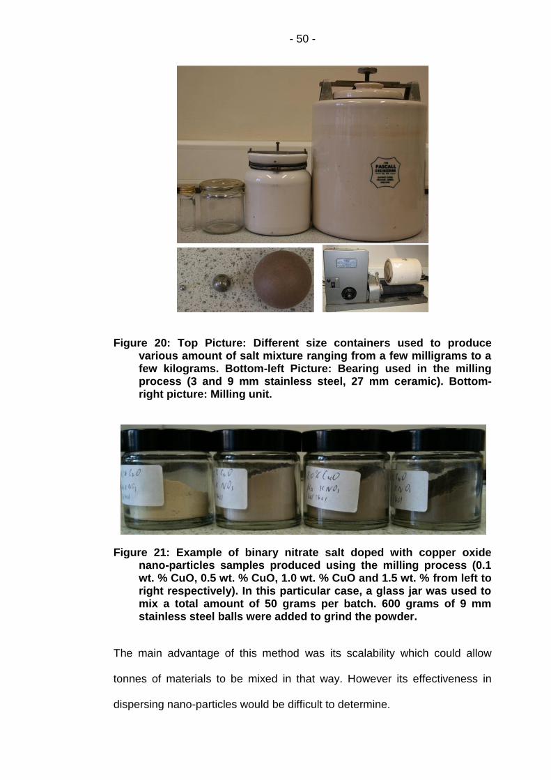
- 50 -

Figure 20: Top Picture: Different size containers used to produce various amount of salt mixture ranging from a few milligrams to a few kilograms. Bottom-left Picture: Bearing used in the milling process (3 and 9 mm stainless steel, 27 mm ceramic). Bottom-right picture: Milling unit.

Figure 21: Example of binary nitrate salt doped with copper oxide nano-particles samples produced using the milling process (0.1 wt. % CuO, 0.5 wt. % CuO, 1.0 wt. % CuO and 1.5 wt. % from left to right respectively). In this particular case, a glass jar was used to mix a total amount of 50 grams per batch. 600 grams of 9 mm stainless steel balls were added to grind the powder.

The main advantage of this method was its scalability which could allow

tonnes of materials to be mixed in that way. However its effectiveness in

dispersing nano-particles would be difficult to determine.

- 51 -

3.3.2 Liquid Process

This method of production involved the dissolution of salts in deionised

water, with nano-particles added to the mix and sonicated for a few hours to

disperse the latter. This was followed by the transfer of this solution into

Petri-dishes for evaporation with further drying to ensure that all the hydrates

were removed. The process which was utilized for the production of

carbonate salt (Section 3.1) was tested with nitrate salt to observe if there

were differences in specific heat capacity between the solid and liquid

method of production. One of the main advantage of this technique was its

ability to allow good dispersion of the nano-particles to be carried out.

However, up-scaling this particular type of production would not be feasible

due to the large expenditure of water and the cost associated to this

process.

3.4 Experimental Procedures

Using differential scanning calorimeter (DSC) (Mettler Toledo, DSC1/700),

thermo-gravimetric analyser (TGA) (Mettler Toledo, LF/1100), scanning

electron microscopy (SEM) (Gemini / Zeiss Leo 1530) and rheometer

(Anton-Paar), various thermo-physical properties of the salts will be tested.

- 52 -

3.4.1 Differential Scanning Calorimeter: Principles &

Methodology

3.4.1.1 Introduction to DSC

This particular apparatus allows the user to analyse the physical or chemical

response taking place within a sample by monitoring the energy changes

occurring throughout heating, cooling or isothermal cycles. It basically tracks

the heat flow into or out of the sample (calorimeter) against that of a

reference (differential) during a constant or dynamic thermal cycle

(scanning) hence the name differential scanning calorimeter (DSC).

Also referred to as enthalpy, these energy changes can be quantitatively

measured and the equipment allows to pin-point at what temperature these

events will occur. The user is therefore able to characterise a range of

chemical or physical changes taking place within the analysed substances

(melting, crystallisation, glass transition, solid-solid transition, enthalpy of

fusion or crystallisation, reaction enthalpy, polymerisation and pyrolysis).

Most of these transitions will either be exothermic or endothermic.

Exothermic: Heat is released from the sample.

Endothermic: Heat is taken into the sample.

The ease of production of sample and the small amount of substances

required makes the use of this equipment a versatile technique which

provides a rapid and efficient way of analysing/characterising any materials.

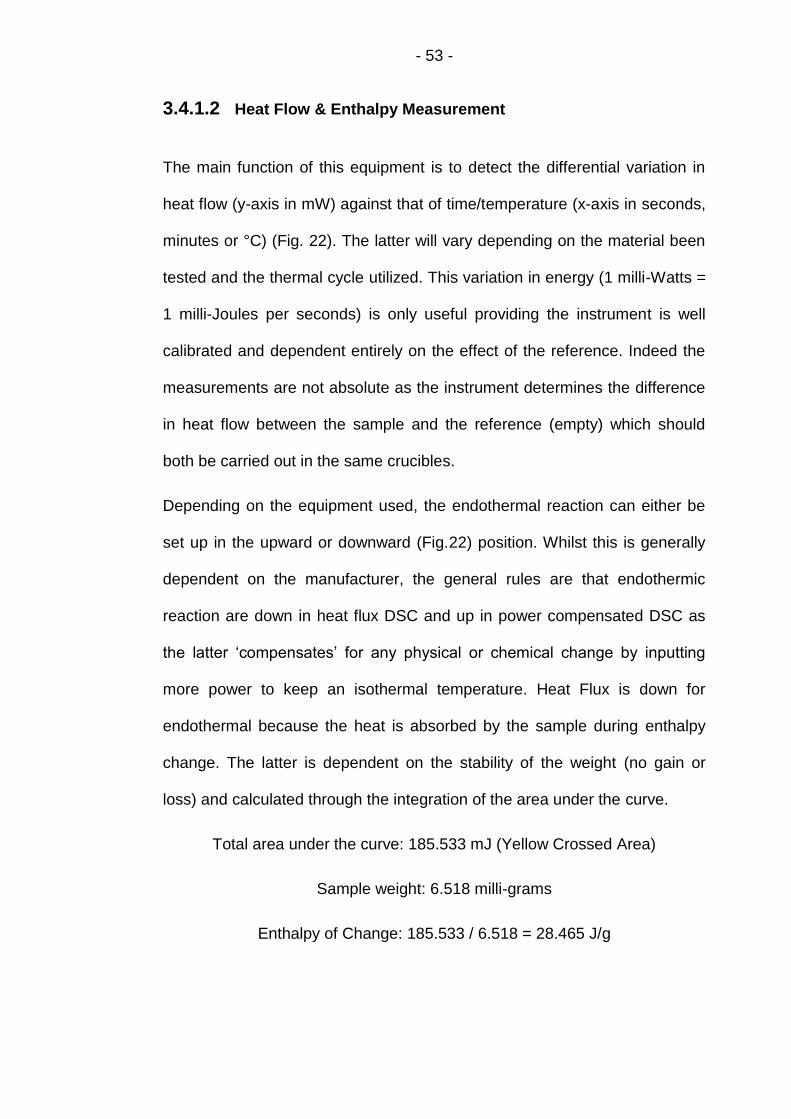
- 53 -

3.4.1.2 Heat Flow & Enthalpy Measurement

The main function of this equipment is to detect the differential variation in

heat flow (y-axis in mW) against that of time/temperature (x-axis in seconds,

minutes or °C) (Fig. 22). The latter will vary depending on the material been

tested and the thermal cycle utilized. This variation in energy (1 milli-Watts =

1 milli-Joules per seconds) is only useful providing the instrument is well

calibrated and dependent entirely on the effect of the reference. Indeed the

measurements are not absolute as the instrument determines the difference

in heat flow between the sample and the reference (empty) which should

both be carried out in the same crucibles.

Depending on the equipment used, the endothermal reaction can either be

set up in the upward or downward (Fig.22) position. Whilst this is generally

dependent on the manufacturer, the general rules are that endothermic

reaction are down in heat flux DSC and up in power compensated DSC as

the latter ‘compensates’ for any physical or chemical change by inputting

more power to keep an isothermal temperature. Heat Flux is down for

endothermal because the heat is absorbed by the sample during enthalpy

change. The latter is dependent on the stability of the weight (no gain or

loss) and calculated through the integration of the area under the curve.

Total area under the curve: 185.533 mJ (Yellow Crossed Area)

Sample weight: 6.518 milli-grams

Enthalpy of Change: 185.533 / 6.518 = 28.465 J/g

- 54 -

Figure 22: Graph displaying Heat Flow (mW) against Time (s) for the melting of Indium

3.4.1.3 Specific Heat Capacity Measurements

The specific heat capacity is referred to as the amount of energy required to

raise the temperature of 1 gram of a substance by 1°C or 1K with units

quoted as J/(g*°C) or J/(g*K). Also designated as Cp, as it is obtained at

constant pressure, the specific heat capacity can be quantitatively measured

using a DSC. The manner in which to achieve that is by measuring the heat

flow of a blank curve, a sapphire standard and a sample on the same

thermal cycles consisting of a dynamic ramp sandwiched between two

isothermal steps (Fig. 23). The blank curve is then manually subtracted from

both the sapphire and the sample (Fig. 24).

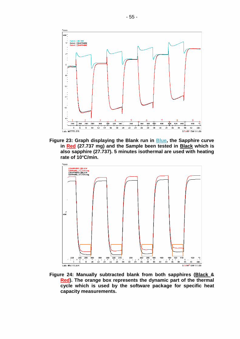
- 55 -

Figure 23: Graph displaying the Blank run in Blue, the Sapphire curve in Red (27.737 mg) and the Sample been tested in Black which is also sapphire (27.737). 5 minutes isothermal are used with heating

rate of 10°C/min.

Figure 24: Manually subtracted blank from both sapphires (Black & Red). The orange box represents the dynamic part of the thermal cycle which is used by the software package for specific heat capacity measurements.

- 56 -

The Mettler Toledo software package allows the user to highlight and

calculate the Cp from the dynamic part of the cycle by boxing and selecting

‘subtracted sample-blank curve’ and ‘sapphire-blank curve’ (Fig. 24).

The software then displays the obtained calculation as specific heat capacity

(J.°C-1.g-1) versus temperature (Fig. 25). The results are usually exported to

excel or origin for further analysis. It is to be noted that the results are taken

a few degrees Celsius after and before the start and end of the dynamic

segment as only the linear part of the curve (Fig. 24: Orange Box) is useful

in the analysis of the data as the equipment needs a bit of time to settle in

this dynamic equilibrium.

Figure 25: Calculated Cp of Sapphire from 261°C to 444°C.

The current setup used to measure Cp follows the ASTM E-1269-05

standard whereby the known value of the sapphire’s Cp standard is used to

calculate the value of measured sample following the equation below:

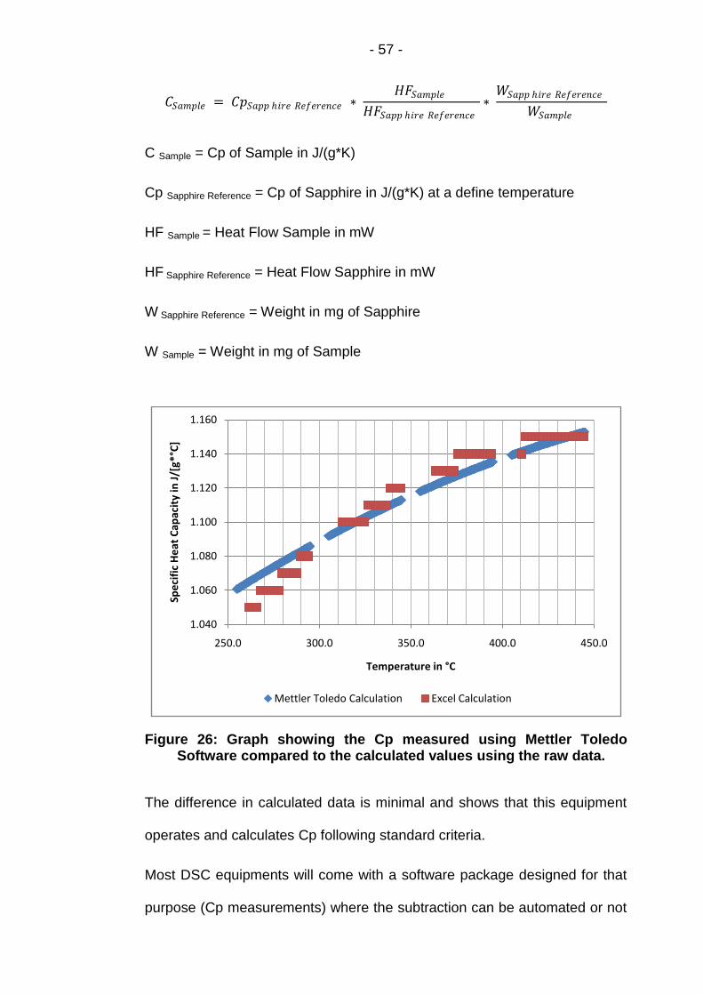
- 57 -

𝐶𝑆𝑎𝑚𝑝𝑙𝑒 = 𝐶𝑝𝑆𝑎𝑝𝑝 ℎ𝑖𝑟𝑒 𝑅𝑒𝑓𝑒𝑟𝑒𝑛𝑐𝑒 ∗ 𝐻𝐹𝑆𝑎𝑚𝑝𝑙𝑒

𝐻𝐹𝑆𝑎𝑝𝑝 ℎ𝑖𝑟𝑒 𝑅𝑒𝑓𝑒𝑟𝑒𝑛𝑐𝑒∗

𝑊𝑆𝑎𝑝𝑝 ℎ𝑖𝑟𝑒 𝑅𝑒𝑓𝑒𝑟𝑒𝑛𝑐𝑒

𝑊𝑆𝑎𝑚𝑝𝑙𝑒

C Sample = Cp of Sample in J/(g*K)

Cp Sapphire Reference = Cp of Sapphire in J/(g*K) at a define temperature

HF Sample = Heat Flow Sample in mW

HF Sapphire Reference = Heat Flow Sapphire in mW

W Sapphire Reference = Weight in mg of Sapphire

W Sample = Weight in mg of Sample

Figure 26: Graph showing the Cp measured using Mettler Toledo Software compared to the calculated values using the raw data.

The difference in calculated data is minimal and shows that this equipment

operates and calculates Cp following standard criteria.

Most DSC equipments will come with a software package designed for that

purpose (Cp measurements) where the subtraction can be automated or not

1.040

1.060

1.080

1.100

1.120

1.140

1.160

250.0 300.0 350.0 400.0 450.0

Spe

cifi

c H

eat

Cap

acit

y in

J/[

g*°C

]

Temperature in °C

Mettler Toledo Calculation Excel Calculation

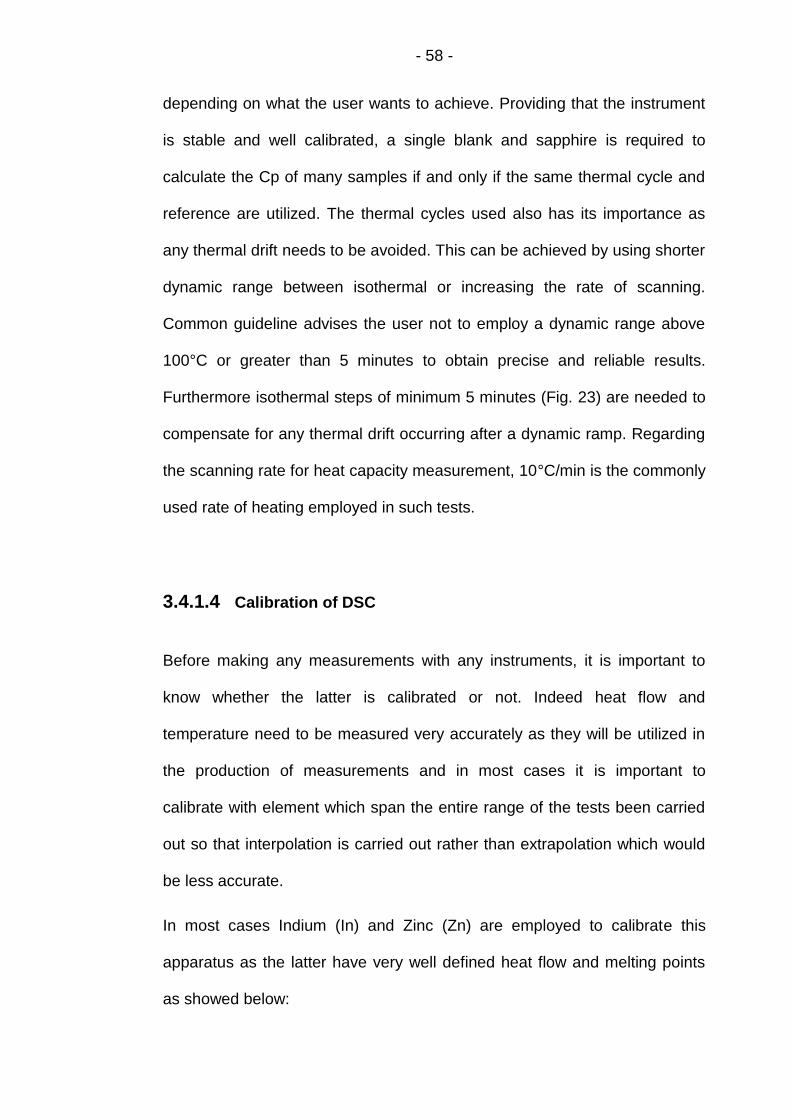
- 58 -

depending on what the user wants to achieve. Providing that the instrument

is stable and well calibrated, a single blank and sapphire is required to

calculate the Cp of many samples if and only if the same thermal cycle and

reference are utilized. The thermal cycles used also has its importance as

any thermal drift needs to be avoided. This can be achieved by using shorter

dynamic range between isothermal or increasing the rate of scanning.

Common guideline advises the user not to employ a dynamic range above

100°C or greater than 5 minutes to obtain precise and reliable results.

Furthermore isothermal steps of minimum 5 minutes (Fig. 23) are needed to

compensate for any thermal drift occurring after a dynamic ramp. Regarding

the scanning rate for heat capacity measurement, 10°C/min is the commonly

used rate of heating employed in such tests.

3.4.1.4 Calibration of DSC

Before making any measurements with any instruments, it is important to

know whether the latter is calibrated or not. Indeed heat flow and

temperature need to be measured very accurately as they will be utilized in

the production of measurements and in most cases it is important to

calibrate with element which span the entire range of the tests been carried

out so that interpolation is carried out rather than extrapolation which would

be less accurate.

In most cases Indium (In) and Zinc (Zn) are employed to calibrate this

apparatus as the latter have very well defined heat flow and melting points

as showed below:

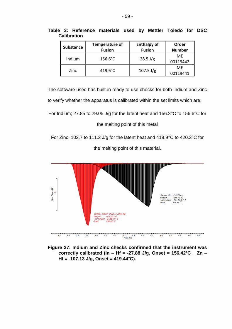
- 59 -

Table 3: Reference materials used by Mettler Toledo for DSC Calibration

Substance Temperature of

Fusion Enthalpy of

Fusion Order

Number

Indium 156.6°C 28.5 J/g ME

00119442

Zinc 419.6°C 107.5 J/g ME

00119441

The software used has built-in ready to use checks for both Indium and Zinc

to verify whether the apparatus is calibrated within the set limits which are:

For Indium; 27.85 to 29.05 J/g for the latent heat and 156.3°C to 156.6°C for

the melting point of this metal

For Zinc; 103.7 to 111.3 J/g for the latent heat and 418.9°C to 420.3°C for

the melting point of this material.

Figure 27: Indium and Zinc checks confirmed that the instrument was

correctly calibrated (In – Hf = -27.88 J/g, Onset = 156.42°C _ Zn –

Hf = -107.13 J/g, Onset = 419.44°C).

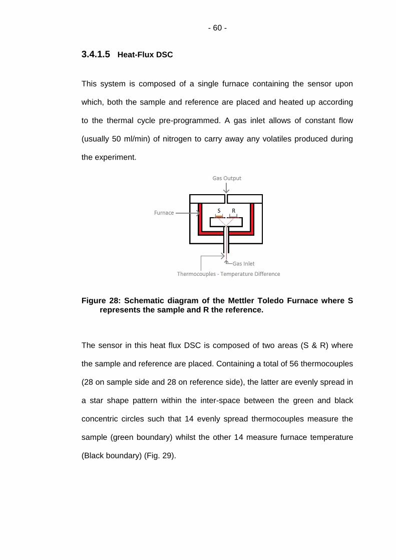
- 60 -

3.4.1.5 Heat-Flux DSC

This system is composed of a single furnace containing the sensor upon

which, both the sample and reference are placed and heated up according

to the thermal cycle pre-programmed. A gas inlet allows of constant flow

(usually 50 ml/min) of nitrogen to carry away any volatiles produced during

the experiment.

Figure 28: Schematic diagram of the Mettler Toledo Furnace where S represents the sample and R the reference.

The sensor in this heat flux DSC is composed of two areas (S & R) where

the sample and reference are placed. Containing a total of 56 thermocouples

(28 on sample side and 28 on reference side), the latter are evenly spread in

a star shape pattern within the inter-space between the green and black

concentric circles such that 14 evenly spread thermocouples measure the

sample (green boundary) whilst the other 14 measure furnace temperature

(Black boundary) (Fig. 29).

- 61 -

Figure 29: Schematic of DSC sensor. Labelled in green (TS& TR) are the areas where the crucibles come into contact with the sensor. The area labelled with the orange arrows is exposed to the chamber.

Based on Georg Ohm law (I = ΔV/Re) which is analogous to Fourier’s law of

heat conduction, the following equation is utilized:

𝑞 = 𝛥𝑇

𝑅

Where q is the heat transferred in watts, ΔT is the temperature difference in

Kelvin or °C whilst R is the resistance K or °C/W. In this system, the heat

flow is impeded by the sample pan, the sample if present and the ceramic

layer covering the thermocouple. Thus R is defined as:

𝑅 = 𝑙

𝑘𝐴

Where l is the length in m, k is the thermal conductivity in W/(m*K or °C) and

A is the area in m2.

In this equipment, the thermocouples average the different in temperature

between the sample and the reference following the equation below:

𝑑𝑞

𝑑𝑡=

1

𝑅 (𝛥𝑇𝑆0)𝑖 −

𝑁

𝑖=1

(𝛥𝑇𝑅0)𝑖

𝑁

𝑖=1

Where N is the number of thermocouple, ΔTS0 equates to difference

between the sample and the furnace temperature whilst ΔTR0 is the

difference in temperature between that of the reference and the furnace.

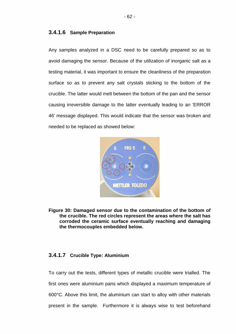
- 62 -

3.4.1.6 Sample Preparation

Any samples analyzed in a DSC need to be carefully prepared so as to

avoid damaging the sensor. Because of the utilization of inorganic salt as a

testing material, it was important to ensure the cleanliness of the preparation

surface so as to prevent any salt crystals sticking to the bottom of the

crucible. The latter would melt between the bottom of the pan and the sensor

causing irreversible damage to the latter eventually leading to an 'ERROR

46' message displayed. This would indicate that the sensor was broken and

needed to be replaced as showed below:

Figure 30: Damaged sensor due to the contamination of the bottom of the crucible. The red circles represent the areas where the salt has corroded the ceramic surface eventually reaching and damaging the thermocouples embedded below.

3.4.1.7 Crucible Type: Aluminium

To carry out the tests, different types of metallic crucible were trialled. The

first ones were aluminium pans which displayed a maximum temperature of

600°C. Above this limit, the aluminium can start to alloy with other materials

present in the sample. Furthermore it is always wise to test beforehand

- 63 -

whether any reactions between the samples and the aluminium might occur

at high temperature to prevent damaging the sensor.

A few samples were prepared in standard 40 µl aluminium pan with their

corresponding top which were pierced with a needle and crimped. This was

done to protect the sensor and prevent any pressure build up which might

have led to the capsules exploding within the furnace.

Figure 31: Composite picture of sample production.

The tests were carried out with 22.000-24.000 mg of samples which were

inserted in the container unless a blank or reference was produced in which

case the crucibles were left empty. Following this the lid was crimped using

Mettler Toledo crimping tool which does not remove any metal in the

process such that the weight of the pan does not vary.

However repeated heating and cooling cycles of the aluminium pan as well

as the force applied on the edge of the crucible by the robotic hand gradually

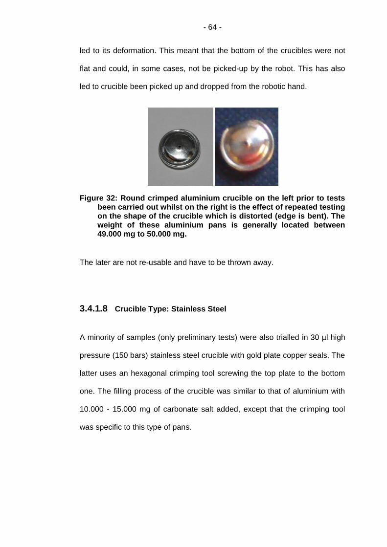
- 64 -

led to its deformation. This meant that the bottom of the crucibles were not

flat and could, in some cases, not be picked-up by the robot. This has also

led to crucible been picked up and dropped from the robotic hand.

Figure 32: Round crimped aluminium crucible on the left prior to tests been carried out whilst on the right is the effect of repeated testing on the shape of the crucible which is distorted (edge is bent). The weight of these aluminium pans is generally located between 49.000 mg to 50.000 mg.

The later are not re-usable and have to be thrown away.

3.4.1.8 Crucible Type: Stainless Steel

A minority of samples (only preliminary tests) were also trialled in 30 µl high

pressure (150 bars) stainless steel crucible with gold plate copper seals. The

latter uses an hexagonal crimping tool screwing the top plate to the bottom

one. The filling process of the crucible was similar to that of aluminium with

10.000 - 15.000 mg of carbonate salt added, except that the crimping tool

was specific to this type of pans.

- 65 -

Figure 33: 30 µl stainless steel high pressure capsule showing the various parts and how they are assembled (a - c).

The production of those samples was closely monitored to prevent the

explosion of the capsule due to a build up in pressure. The latter would have

had a catastrophic effect on the DSC sensor. As salt can absorb moisture

from the air over time and because of the high vapour pressure of water, it

was crucial to melt the samples before sealing them to minimize the

entrapment of water moisture. This type of crucible could only be re-used for

a couple of tests and problem with leaking of sealed capsules was the major

concern when using the latter.

3.4.1.9 Crucible Type: Platinum

The majority of tests were carried out with platinum pans. They display very

high melting point, are resistant to corrosion, do not suffer from distortion

upon repeated heating & cooling and were not affect by the robotic hand

always keeping the same shape.

a

b c

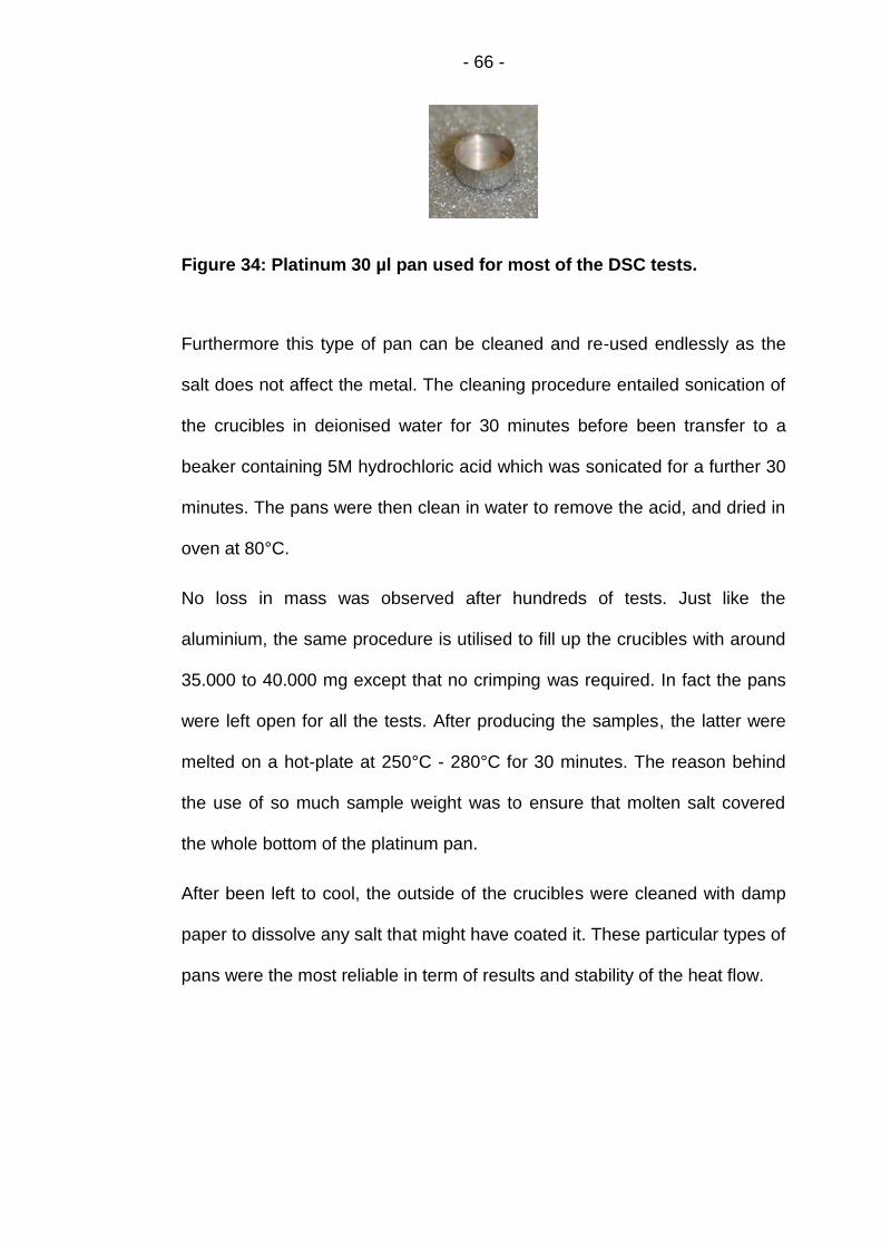
- 66 -

Figure 34: Platinum 30 µl pan used for most of the DSC tests.

Furthermore this type of pan can be cleaned and re-used endlessly as the

salt does not affect the metal. The cleaning procedure entailed sonication of

the crucibles in deionised water for 30 minutes before been transfer to a

beaker containing 5M hydrochloric acid which was sonicated for a further 30

minutes. The pans were then clean in water to remove the acid, and dried in

oven at 80°C.

No loss in mass was observed after hundreds of tests. Just like the

aluminium, the same procedure is utilised to fill up the crucibles with around

35.000 to 40.000 mg except that no crimping was required. In fact the pans

were left open for all the tests. After producing the samples, the latter were

melted on a hot-plate at 250°C - 280°C for 30 minutes. The reason behind

the use of so much sample weight was to ensure that molten salt covered

the whole bottom of the platinum pan.

After been left to cool, the outside of the crucibles were cleaned with damp

paper to dissolve any salt that might have coated it. These particular types of

pans were the most reliable in term of results and stability of the heat flow.

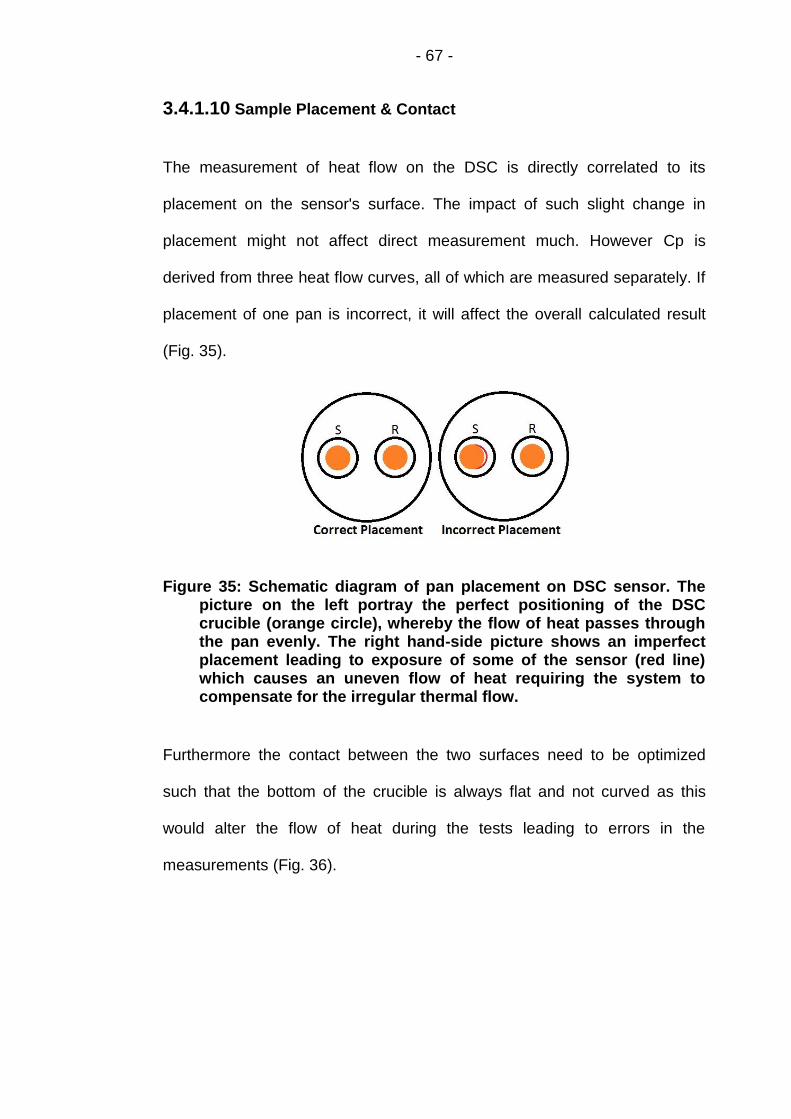
- 67 -

3.4.1.10 Sample Placement & Contact

The measurement of heat flow on the DSC is directly correlated to its

placement on the sensor's surface. The impact of such slight change in

placement might not affect direct measurement much. However Cp is

derived from three heat flow curves, all of which are measured separately. If

placement of one pan is incorrect, it will affect the overall calculated result

(Fig. 35).

Figure 35: Schematic diagram of pan placement on DSC sensor. The picture on the left portray the perfect positioning of the DSC crucible (orange circle), whereby the flow of heat passes through the pan evenly. The right hand-side picture shows an imperfect placement leading to exposure of some of the sensor (red line) which causes an uneven flow of heat requiring the system to compensate for the irregular thermal flow.

Furthermore the contact between the two surfaces need to be optimized

such that the bottom of the crucible is always flat and not curved as this

would alter the flow of heat during the tests leading to errors in the

measurements (Fig. 36).

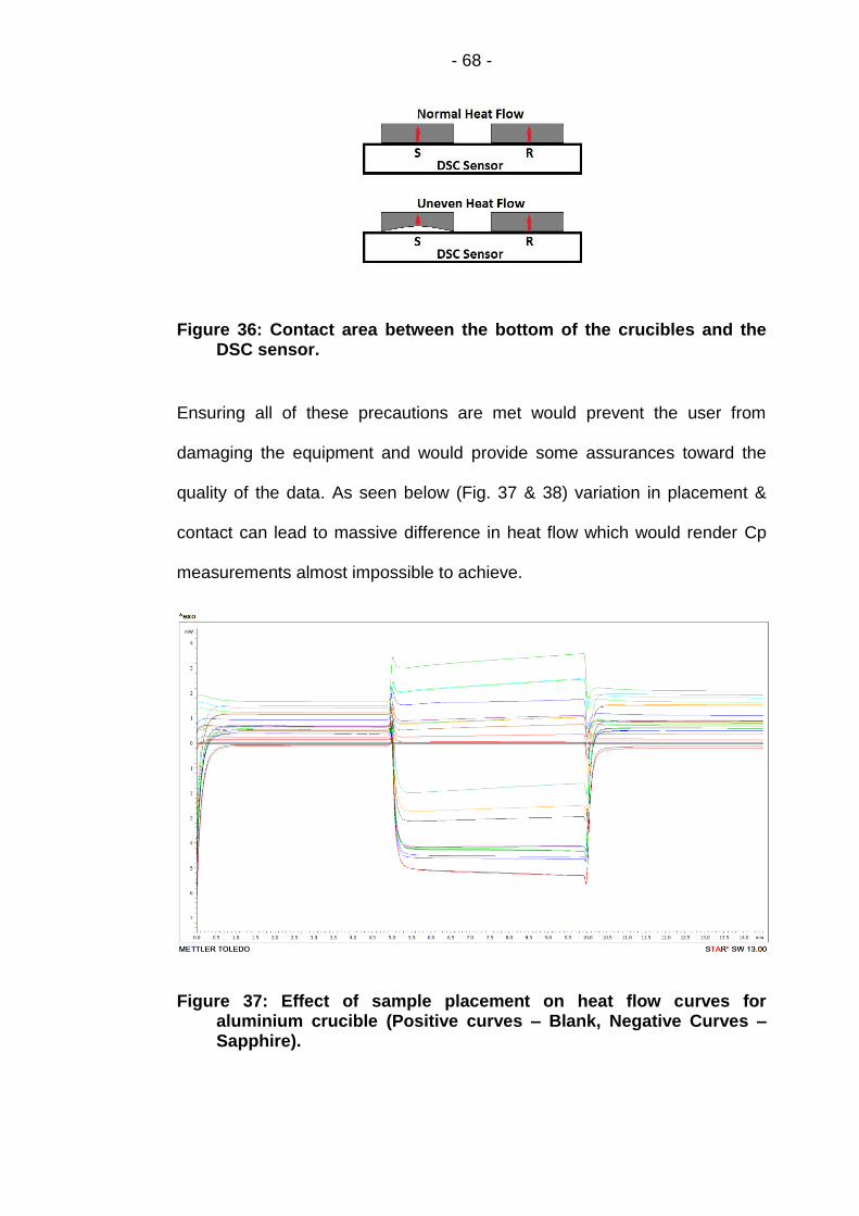
- 68 -

Figure 36: Contact area between the bottom of the crucibles and the DSC sensor.

Ensuring all of these precautions are met would prevent the user from

damaging the equipment and would provide some assurances toward the

quality of the data. As seen below (Fig. 37 & 38) variation in placement &

contact can lead to massive difference in heat flow which would render Cp

measurements almost impossible to achieve.

Figure 37: Effect of sample placement on heat flow curves for aluminium crucible (Positive curves – Blank, Negative Curves – Sapphire).

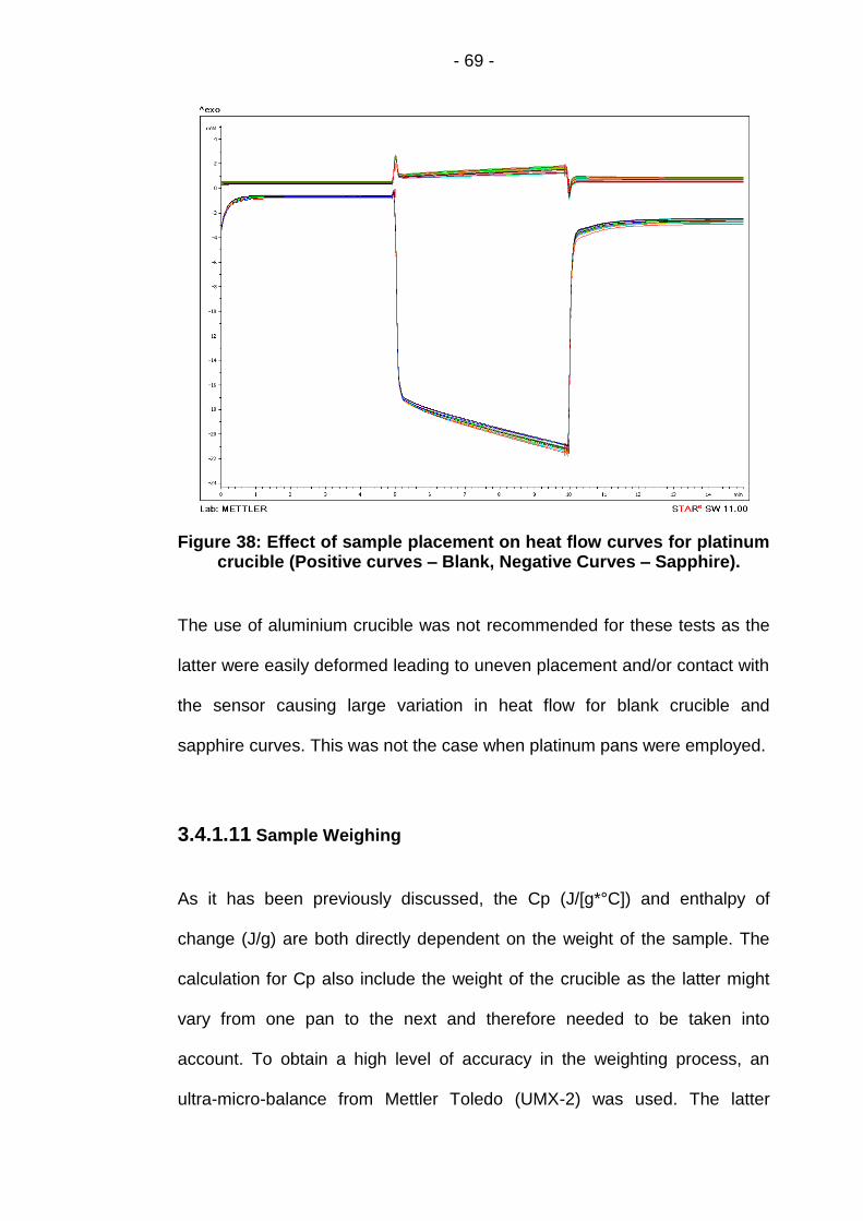
- 69 -

Figure 38: Effect of sample placement on heat flow curves for platinum crucible (Positive curves – Blank, Negative Curves – Sapphire).

The use of aluminium crucible was not recommended for these tests as the

latter were easily deformed leading to uneven placement and/or contact with

the sensor causing large variation in heat flow for blank crucible and

sapphire curves. This was not the case when platinum pans were employed.

3.4.1.11 Sample Weighing

As it has been previously discussed, the Cp (J/[g*°C]) and enthalpy of

change (J/g) are both directly dependent on the weight of the sample. The

calculation for Cp also include the weight of the crucible as the latter might

vary from one pan to the next and therefore needed to be taken into

account. To obtain a high level of accuracy in the weighting process, an

ultra-micro-balance from Mettler Toledo (UMX-2) was used. The latter

- 70 -

displayed an accuracy of 1.0 µg. Both samples and pans weight were

recorded and used in the characterisation of the salts.

Figure 39: Ultra-micro-balance set on a granite block and encased in a plastic box to reduce the vibrations coming from the surrounding.

3.4.1.12 Thermal Cycles for DSC

The creation of a thermal cycle needs to be suited to what the user wants to

achieve. In this research, the main point of interest was Cp but

characteristics such as enthalpy and temperature at which transition from

liquid to solid occurred were also analysed.

The value of Cp was tested between 250°C to 450°C with two different

cycles where thermal cycle 1 was set with a heating rate of 10°C/min whilst

thermal cycle 2 was programmed with a ramp of 40°C/min. Both used 5

minutes isothermal to surround each ramp.

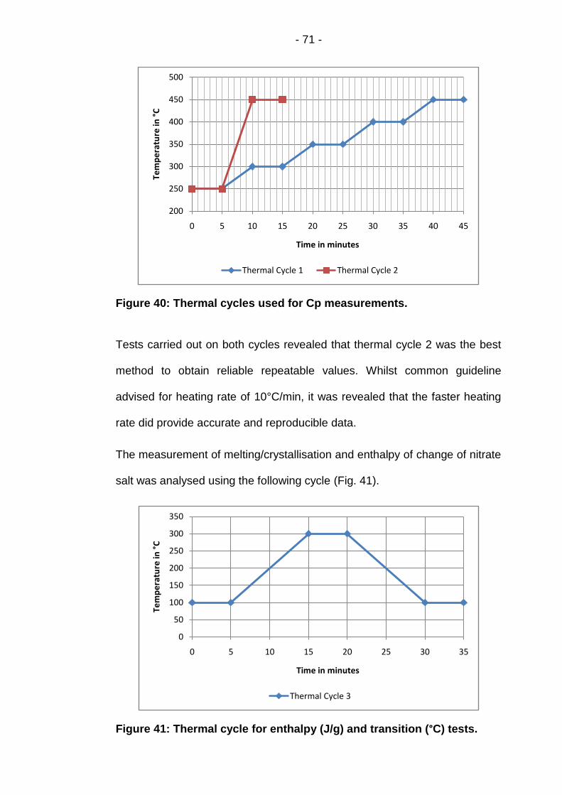
- 71 -

Figure 40: Thermal cycles used for Cp measurements.

Tests carried out on both cycles revealed that thermal cycle 2 was the best

method to obtain reliable repeatable values. Whilst common guideline

advised for heating rate of 10°C/min, it was revealed that the faster heating

rate did provide accurate and reproducible data.

The measurement of melting/crystallisation and enthalpy of change of nitrate

salt was analysed using the following cycle (Fig. 41).

Figure 41: Thermal cycle for enthalpy (J/g) and transition (°C) tests.

200

250

300

350

400

450

500

0 5 10 15 20 25 30 35 40 45

Tem

pe

ratu

re in

°C

Time in minutes

Thermal Cycle 1 Thermal Cycle 2

0

50

100

150

200

250

300

350

0 5 10 15 20 25 30 35

Tem

pe

ratu

re in

°C

Time in minutes

Thermal Cycle 3

- 72 -

3.4.2 Thermo-gravimetric Analyser: Principles & Methodology

3.4.2.1 Introduction to TGA

The primary function of this apparatus is to measure change in mass as a

function of either temperature (with constant heating rate usually

10°C/minute) or time (constant temperature) in a controlled atmosphere.

Many changes whether physical or chemical such as sublimation,

evaporation, absorption, adsorption, oxidation or reduction will affect the

weight of a sample either positively or negatively.

Figure 42: Schematic diagram of the TGA from Mettler Toledo.

Operating at temperature ranging from 25°C to 1100°C, the furnace is

opened, exposing the sample holder where the crucible is placed onto. Prior

to sample insertion, the pans and sample weights are recorded on the Ultra-

- 73 -

micro-balance to verify that there are no discrepancies in weight between

the two equipments (Resolution of 1.0 µg). The advantage of such system

lays in the fact that measurement can be done up to 1100°C which is not the

case of a normal DSC system as it is restricted to 700°C. However the

precision obtained with a single DSC system surpass that of a combined

DSC/TGA.

3.4.2.2 Balance and Heat Flow Calibration

The instrument’s ultra-micro-balance contains two internal weights which

automatically calibrates the system when it is turned on. External calibration

can also be done with standard weight obtained from Mettler Toledo but this

step was not carried out as both ultra-micro-balances gave similar weight

reading when weighting the samples.

Heat flow calibration is done through a similar inbuilt system to that of the

DSC. However the calibration of this system requires the testing of 4 metals

(Indium, Zinc, Aluminium and Gold) that span the entire range of the

equipment.

Table 4: TGA/DSC Calibration Metals

Material

Melting Range Melting Temperature

Heat of Fusion Range

Heat of

Fusion

°C °C J/g J/g

Indium 155.1 - 158.1 (156.6°C)

157.13 24.225 - 32.775 (28.5 J/g)

30.04

Zinc 417.5 - 421.5 (419.5°C)

420.03 91.375 - 123.625 (107.5 J/g)

113.53

Aluminium 657.8 - 662.8 (660.3°C)

660.53 317.6 - 476.4 (397.0 J/g)

386.11

Gold 1061.2 - 1067.2 (1064.2°C)

1065.06 50.96 - 76.44 (63.7 J/g)

67.79

- 74 -

3.4.2.3 Crucible Type and Sample Preparation

The choice of crucible needed to be appropriate to the experiment been

conducted with the TGA. In most cases, alumina samples would be used as

this material can easily withstand the maximum temperature (1100°C).

However, it was discovered that the porosity of the alumina crucible led to

the infiltration of salt through to the sample holder’s surface. This led to the

inability to remove the pan due to crystallisation occurring between the two

surfaces. To dislodge the crucible, the whole sample holder plus the crucible

were removed and placed in deionised water to dissolve the salt. To prevent

this, platinum crucibles were used as they can withstand high temperature

(>1100°C) and are very resistant to corrosion. Furthermore they are not

porous.

Thermal stability tests of the salt were conducted by using 10.000 to 15.000

mg of sample loaded inside the platinum pans. The crucible were placed

onto the carousel and the experiment were programmed. The thermal cycle

used was as followed:

Isothermal at 50°C for 20 minutes

Dynamic from 50°C to 1000°C at 10°C/min

- 75 -

3.4.3 Scanning Electron Microscopy

This system (LEO 1530) was used to analyse the crystallised molten salt

surface and investigate whether or not nano-particles were present to see

how the latter adhered to the crystal’s surface. Using an electron beam,

SEM analysis allows the user to reach resolution within the nano-meters

range. Samples tested on the DSC using aluminium pans were cut open and

stuck onto an SEM stub. The latter was usually coated with a platinum layer

of 5 nm before analysis was to start. Due to the inability to control size and

shape of the sample, most analyses were carried out on uneven surface.

Figure 43: Schematic Diagram of SEM

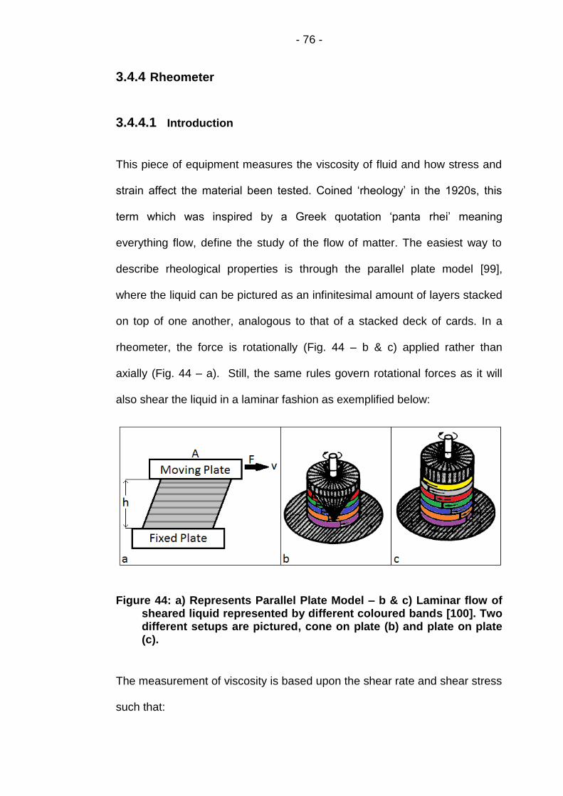
- 76 -

3.4.4 Rheometer

3.4.4.1 Introduction

This piece of equipment measures the viscosity of fluid and how stress and

strain affect the material been tested. Coined ‘rheology’ in the 1920s, this

term which was inspired by a Greek quotation ‘panta rhei’ meaning

everything flow, define the study of the flow of matter. The easiest way to

describe rheological properties is through the parallel plate model [99],

where the liquid can be pictured as an infinitesimal amount of layers stacked

on top of one another, analogous to that of a stacked deck of cards. In a

rheometer, the force is rotationally (Fig. 44 – b & c) applied rather than

axially (Fig. 44 – a). Still, the same rules govern rotational forces as it will

also shear the liquid in a laminar fashion as exemplified below:

Figure 44: a) Represents Parallel Plate Model – b & c) Laminar flow of sheared liquid represented by different coloured bands [100]. Two different setups are pictured, cone on plate (b) and plate on plate (c).

The measurement of viscosity is based upon the shear rate and shear stress

such that:

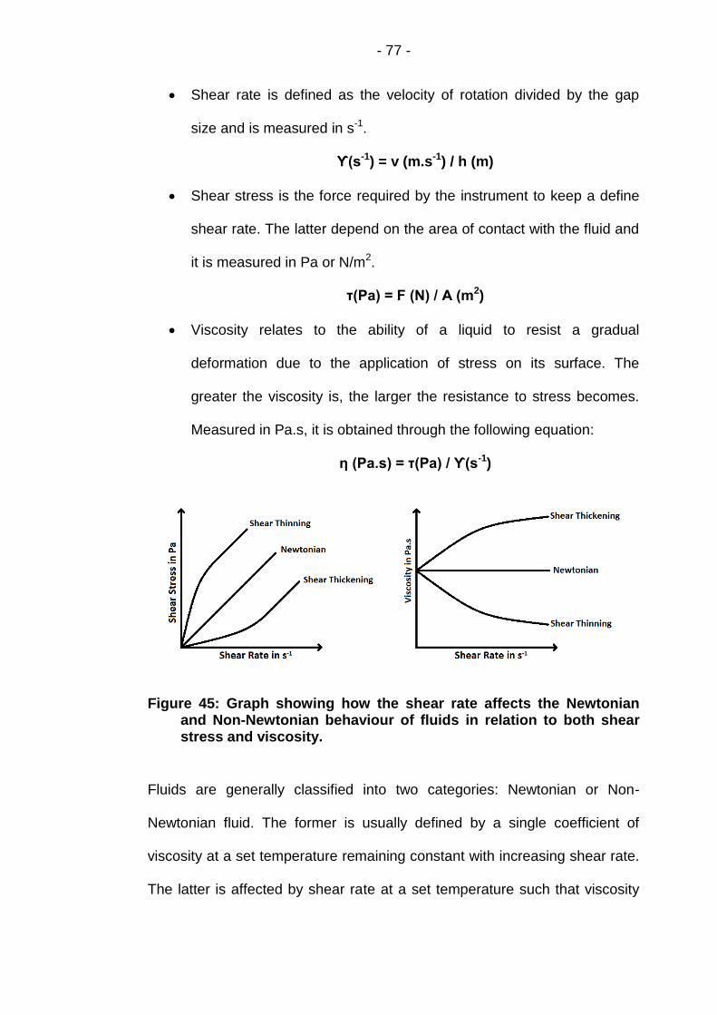
- 77 -

Shear rate is defined as the velocity of rotation divided by the gap

size and is measured in s-1.

ϒ(s-1) = v (m.s-1) / h (m)

Shear stress is the force required by the instrument to keep a define

shear rate. The latter depend on the area of contact with the fluid and

it is measured in Pa or N/m2.

τ(Pa) = F (N) / A (m2)

Viscosity relates to the ability of a liquid to resist a gradual

deformation due to the application of stress on its surface. The

greater the viscosity is, the larger the resistance to stress becomes.

Measured in Pa.s, it is obtained through the following equation:

η (Pa.s) = τ(Pa) / ϒ(s-1)

Figure 45: Graph showing how the shear rate affects the Newtonian and Non-Newtonian behaviour of fluids in relation to both shear stress and viscosity.

Fluids are generally classified into two categories: Newtonian or Non-

Newtonian fluid. The former is usually defined by a single coefficient of

viscosity at a set temperature remaining constant with increasing shear rate.

The latter is affected by shear rate at a set temperature such that viscosity

- 78 -

will either increase or decrease causing either shear-thinning or shear-

thickening of the material in question.

3.4.4.2 Cone or Flat Plate Setup

The geometry of the setup will affect the measurement as the shear stress is

related to the area of contact. In a plate-plate system, the shear rate is not

constant across the radius such that the edge of the plate experiences

maximum velocity whilst the centre displays a velocity of zero. Furthermore

the gap can be altered and depends on the material been tested. In a cone-

plate, the shear rate is uniform across the radius and the gap is pre-set to a

certain standard which depend on the manufacturer. Both system use small

volume and are easy to clean, but the fact that it was not known how shear

rate would affect the material favoured the cone and plate model. Calibration

test with plate-plate setup were not convincing and determining a gap size

which provided accurate data was difficult to achieve hence this type of

setup was discarded.

3.4.4.3 Setup

Viscosity measurements were carried out with an Anton Paar ‘Physica MCR

301 TruGap Ready’ fitted with a furnace and a ‘TC30’ temperature controller

unit (Accurate to 0.1°C). The nature of the sample tested required high

temperature to melt the sample into its liquid form before testing could begin.

However prior to any measurements been made, the rheometer had to be

tested with standard both at low and high temperature to ensure that both

- 79 -

the instrument and this particular setup utilized were calibrated and providing

the correct results.

Figure 46: Rheometer setup used to measure viscosity of molten salt. The left picture shows the open two halves of the furnace, with in the middle, either a 65 or 50 mm stainless steel plate onto which the sample is placed with an over-hanging stainless steel cone of 50 mm diameter and 1° angle. The right picture is the setup of the equipment once the furnace is closed.

Using water, standard oil and published viscosity data from KNO3, the

rheometer was checked to ensure that it was calibrated before any of the

tests were started. As a cone and plate setup was utilized, the gap between

the plate and the flat tip of the cone was pre-set at 0.098 mm. In order to

achieve the test, it is crucial to have the correct amount of liquid in the gap

such that the whole area of the cone (just the underside) is used, however,

too much or too little liquid would lead to a greater or smaller area of contact,

increasing or decreasing the value of viscosity providing misleading

information.

- 80 -

Figure 47: Schematic diagram of the area of contact between the liquid and the cone & plate setup. Diagram a) has too little fluid between the plate & cone, whilst b) has too much such that the edge of the cone is taken into account (orange circles). Only c) would provide the correct value as only the underside of the cone is utilized for the measurements.

The preset volume required is 0.57 ml which is the equivalent of 0.57 cm3

providing the density is 1.00 g/cm3. Therefore, if the density of the liquid is

known, it is possible to back-calculate the amount needed. The calibration

with the mentioned above substances will provide the user with the

assurance that the correct volume/amount is used.

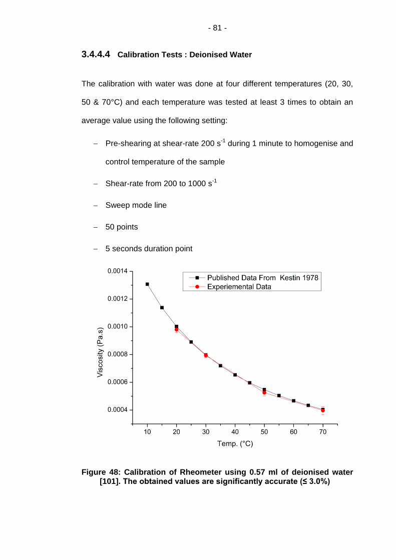
- 81 -

3.4.4.4 Calibration Tests : Deionised Water

The calibration with water was done at four different temperatures (20, 30,

50 & 70°C) and each temperature was tested at least 3 times to obtain an

average value using the following setting:

Pre-shearing at shear-rate 200 s-1 during 1 minute to homogenise and

control temperature of the sample

Shear-rate from 200 to 1000 s-1

Sweep mode line

50 points

5 seconds duration point

Figure 48: Calibration of Rheometer using 0.57 ml of deionised water [101]. The obtained values are significantly accurate (≤ 3.0%)

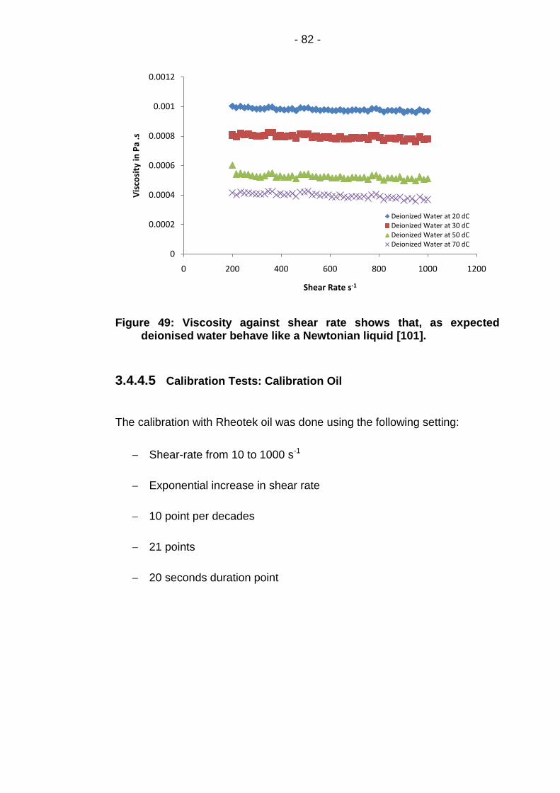
- 82 -

Figure 49: Viscosity against shear rate shows that, as expected deionised water behave like a Newtonian liquid [101].

3.4.4.5 Calibration Tests: Calibration Oil

The calibration with Rheotek oil was done using the following setting:

Shear-rate from 10 to 1000 s-1

Exponential increase in shear rate

10 point per decades

21 points


0

0.0002

0.0004

0.0006

0.0008

0.001

0.0012

0 200 400 600 800 1000 1200

Vis

cosi

ty in

Pa

.s

Shear Rate s-1

Deionized Water at 20 dCDeionized Water at 30 dCDeionized Water at 50 dCDeionized Water at 70 dC

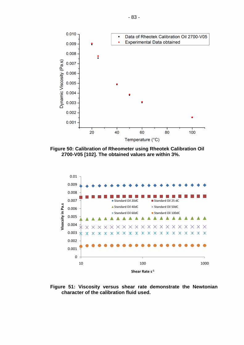
- 83 -

Figure 50: Calibration of Rheometer using Rheotek Calibration Oil 2700-V05 [102]. The obtained values are within 3%.

Figure 51: Viscosity versus shear rate demonstrate the Newtonian character of the calibration fluid used.

0

0.001

0.002

0.003

0.004

0.005

0.006

0.007

0.008

0.009

0.01

10 100 1000

Vis

ocs

ity

in P

a.s

Shear Rate s-1

Standard Oil 20dC Standard Oil 25 dC

Standard Oil 40dC Standard Oil 50dC

Standard Oil 60dC Standard Oil 100dC

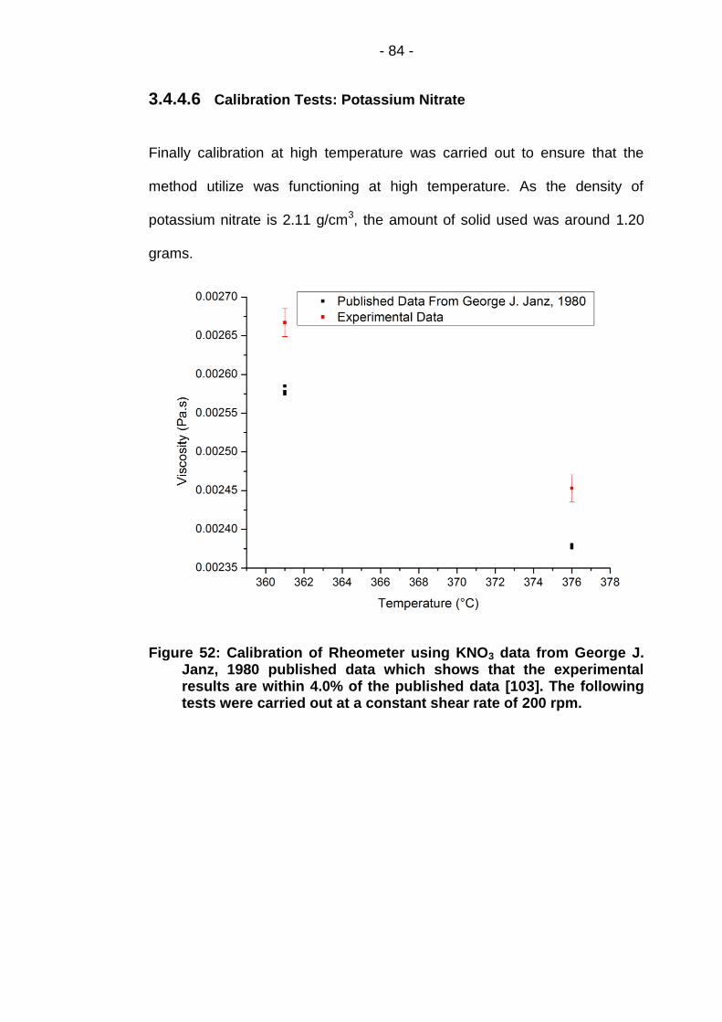
- 84 -

3.4.4.6 Calibration Tests: Potassium Nitrate

Finally calibration at high temperature was carried out to ensure that the

method utilize was functioning at high temperature. As the density of

potassium nitrate is 2.11 g/cm3, the amount of solid used was around 1.20

grams.

Figure 52: Calibration of Rheometer using KNO3 data from George J. Janz, 1980 published data which shows that the experimental results are within 4.0% of the published data [103]. The following tests were carried out at a constant shear rate of 200 rpm.

- 85 -

3.4.4.7. Sample Preparation for Rheological Tests

1.07 grams of powdered salt (density of NaNO3/KNO3 - 60/40, ≈1.89 g/cm3)

was placed onto the plate. The furnace was closed, brought to 250°C, the

cone was lowered to measuring height (0.98 mm) and the tests were started.

The following setting were used for the tests:

Shear-rate cycle from 100 to 1000 s-1 – 1000 to 100 s-1

Cycle Repeated 10 times.

Exponential increase & decrease in shear rate

10 point per decades

11 points


The whole rheometer was programmed to carry a number of tests at set

temperature ranging from 250°C to 450°C.

- 86 -

Chapter 4 Design and Production of Stability Rigs

This chapter describes how and why the stability rigs were created.

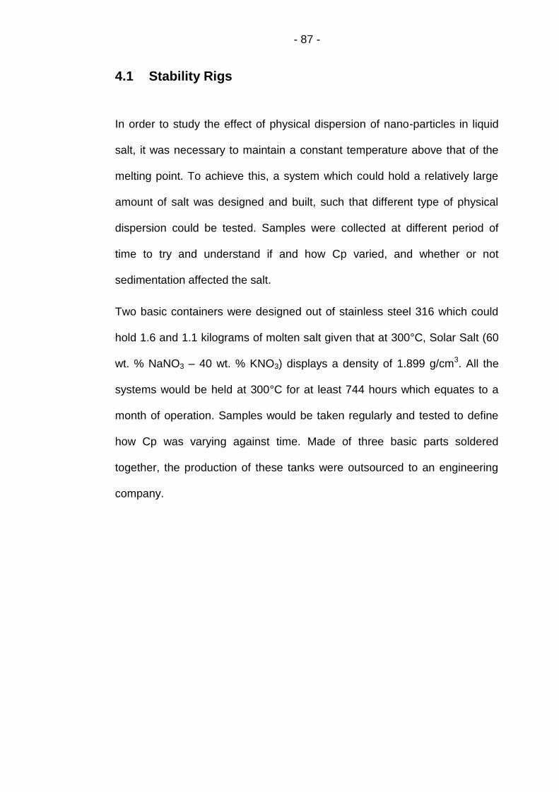
- 87 -

4.1 Stability Rigs

In order to study the effect of physical dispersion of nano-particles in liquid

salt, it was necessary to maintain a constant temperature above that of the

melting point. To achieve this, a system which could hold a relatively large

amount of salt was designed and built, such that different type of physical

dispersion could be tested. Samples were collected at different period of

time to try and understand if and how Cp varied, and whether or not

sedimentation affected the salt.

Two basic containers were designed out of stainless steel 316 which could

hold 1.6 and 1.1 kilograms of molten salt given that at 300°C, Solar Salt (60

wt. % NaNO3 – 40 wt. % KNO3) displays a density of 1.899 g/cm3. All the

systems would be held at 300°C for at least 744 hours which equates to a

month of operation. Samples would be taken regularly and tested to define

how Cp was varying against time. Made of three basic parts soldered

together, the production of these tanks were outsourced to an engineering

company.

- 88 -

4.2 Schematic Design of the 1.6 kg container:

Figure 53: The left-hand side represents the dimensions of each of the parts required to produce the tank shown as a 3D sketch on the top-right hand side with the fully build version seen below it.

Four rigs were built using this particular design:

Static Rig with Pure Salt (100% Solar Salt) (Negative control)

Static Rig with Mixture (Positive control)

Stirring Rig

Bubbling Rig

The top plate for each rig was altered to accommodate the different method

of dispersion utilized.

- 89 -

Figure 54: Schematic diagram of the top-plate.

In both static rigs, the centre hole was removed as no dispersion of any kind

was done. Both of these rigs provided the user with a positive and negative

control to compare the other results to.

For the stirring rig, an overhead low shear rate mixer was used with a shaft

and an axial top-to-bottom impeller blade to provide turbulences (Dimension

of the blade are quotes on Figure 55). The centre hole had to be enlarged to

ensure that the shaft did not come into contact with the top plate so as to

prevent any damage over time.

The bubbling rig had Swagelok fitting to hold a 3.00 mm outer diameter tube.

The centre hole was threaded to fix the whole system in place. Unlike the

photo showed (Fig. 56), the tube was not straight but coiled in shape to allow

the gas to warm up as it descended into the bottom piece where the bubbles

were expelled.

- 90 -

Figure 55: Left: Dimension of the impeller blade used. Right: Overhead Stirrer BDC2010 from Caframo utilized in the stirring rig.

Figure 56: Left: Diagram of the bubbling piece which is centred at the bottom of the tank. Right: Bubbling piece (Red Arrow) connected to 3.0 mm outer diameter tube (Green Arrow) through Swagelok fitting (Orange Line).

- 91 -

4.3 Schematic Diagram for 1.1 kg container:

This system was designed to produce turbulence in the fluid by forcing it to

go through holes located in the centrepiece of the moving cylinder.

Figure 57: Left: Dimension of each of the three parts soldered together. Top-Right: Dimension of the moving centre-piece providing turbulence in the molten fluid. Bottom-Right: Moving centre-piece in orange is connected to a shaft (blue) which is itself linked to a pneumatic piston providing an up and down motion.

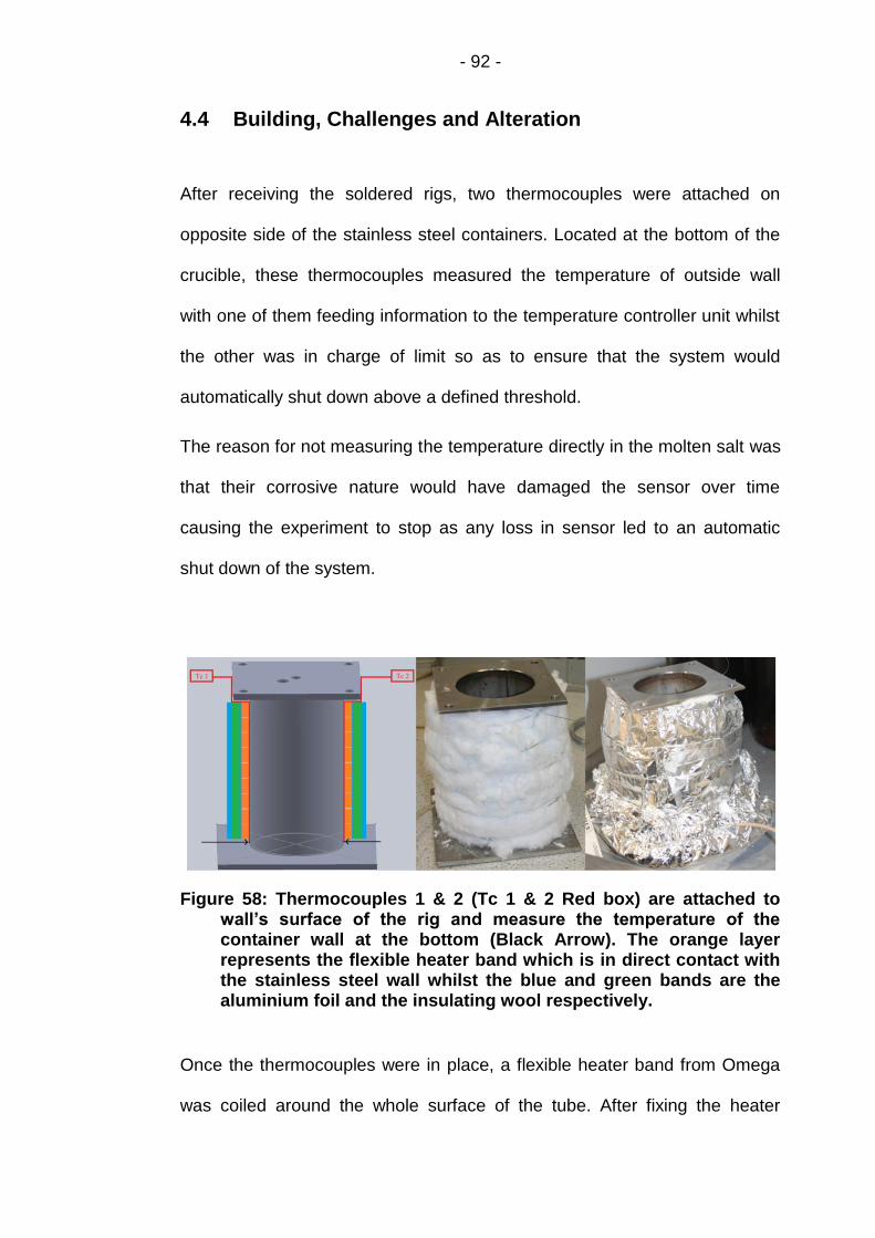
- 92 -

4.4 Building, Challenges and Alteration

After receiving the soldered rigs, two thermocouples were attached on

opposite side of the stainless steel containers. Located at the bottom of the

crucible, these thermocouples measured the temperature of outside wall

with one of them feeding information to the temperature controller unit whilst

the other was in charge of limit so as to ensure that the system would

automatically shut down above a defined threshold.

The reason for not measuring the temperature directly in the molten salt was

that their corrosive nature would have damaged the sensor over time

causing the experiment to stop as any loss in sensor led to an automatic

shut down of the system.

Figure 58: Thermocouples 1 & 2 (Tc 1 & 2 Red box) are attached to wall’s surface of the rig and measure the temperature of the container wall at the bottom (Black Arrow). The orange layer represents the flexible heater band which is in direct contact with the stainless steel wall whilst the blue and green bands are the aluminium foil and the insulating wool respectively.

Once the thermocouples were in place, a flexible heater band from Omega

was coiled around the whole surface of the tube. After fixing the heater

- 93 -

band, aluminium foil was wrapped on top of the heater band so as to allow

heat to escape to prevent the formation of hotspots which would damage the

heater. Finally, insulating wool was used to reduce heat loss followed by

another layer of aluminium foil as seen on Figure 58.

Upon completion of the build, the rig was connected to power unit which was

itself controlled by a lab-view program. In these tests the aim was to roughly

stabilise the temperature at 300°C. Because each rigs was build manually,

the amount of insulation and the placement of the thermocouple were

slightly different which led to different power output been needed to maintain

a constant temperature. This was achieved by manually controlling the

power output of each rig. Once set to a certain power, it was left as such

during the entire length of the tests.

Preliminary empty tests lasting at least 48 hours were carried out to ensure

that the heater could maintain that temperature without failing. On a couple

of occasions, hotspot formation led to the dismantling and re-building of the

rigs. Following on, 600 grams of salt were inserted inside the rigs and

brought up to temperature. After leaving the rigs for a couple of hours, loss

in power was noticed. This was caused by badly soldered joins leading to

salt leaking from the bottom of the rig, and destroying to heater band

causing it to short-circuit. Thus the rigs were sent back.

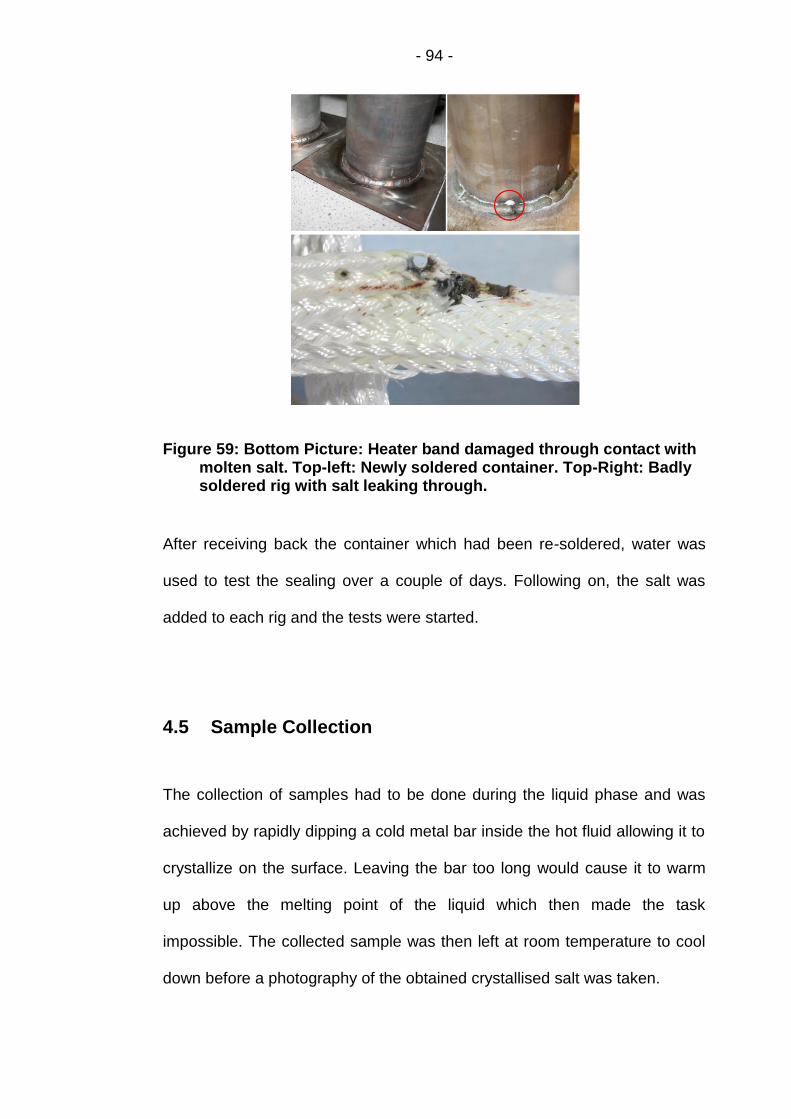
- 94 -

Figure 59: Bottom Picture: Heater band damaged through contact with molten salt. Top-left: Newly soldered container. Top-Right: Badly soldered rig with salt leaking through.

After receiving back the container which had been re-soldered, water was

used to test the sealing over a couple of days. Following on, the salt was

added to each rig and the tests were started.

4.5 Sample Collection

The collection of samples had to be done during the liquid phase and was

achieved by rapidly dipping a cold metal bar inside the hot fluid allowing it to

crystallize on the surface. Leaving the bar too long would cause it to warm

up above the melting point of the liquid which then made the task

impossible. The collected sample was then left at room temperature to cool

down before a photography of the obtained crystallised salt was taken.

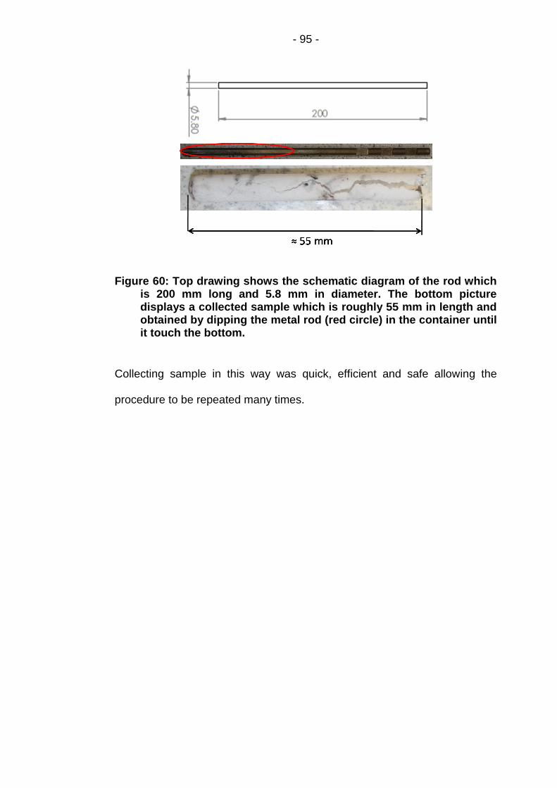
- 95 -

Figure 60: Top drawing shows the schematic diagram of the rod which is 200 mm long and 5.8 mm in diameter. The bottom picture displays a collected sample which is roughly 55 mm in length and obtained by dipping the metal rod (red circle) in the container until it touch the bottom.

Collecting sample in this way was quick, efficient and safe allowing the

procedure to be repeated many times.

- 96 -

Chapter 5 Results & Discussion: Salt Characterisation

without Additives

This chapter provides the user with the data obtained on the characterization

of both single salts sodium & potassium nitrate as well as its eutectic mixture

(60 wt% NaNO3 + 40 wt% KNO3).

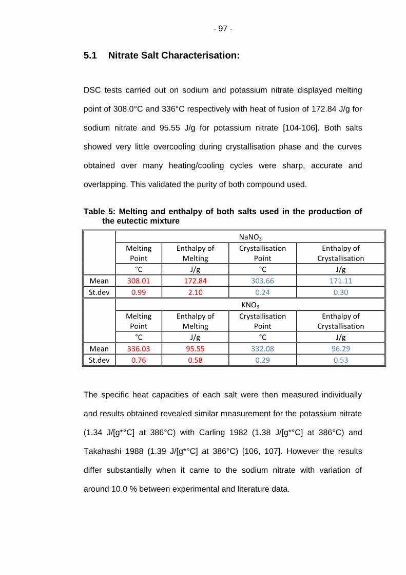
- 97 -

5.1 Nitrate Salt Characterisation:

DSC tests carried out on sodium and potassium nitrate displayed melting

point of 308.0°C and 336°C respectively with heat of fusion of 172.84 J/g for

sodium nitrate and 95.55 J/g for potassium nitrate [104-106]. Both salts

showed very little overcooling during crystallisation phase and the curves

obtained over many heating/cooling cycles were sharp, accurate and

overlapping. This validated the purity of both compound used.

Table 5: Melting and enthalpy of both salts used in the production of the eutectic mixture

NaNO3

Melting

Point Enthalpy of

Melting Crystallisation

Point Enthalpy of

Crystallisation

°C J/g °C J/g

Mean 308.01 172.84 303.66 171.11

St.dev 0.99 2.10 0.24 0.30

KNO3

Melting

Point Enthalpy of

Melting Crystallisation

Point Enthalpy of

Crystallisation

°C J/g °C J/g

Mean 336.03 95.55 332.08 96.29

St.dev 0.76 0.58 0.29 0.53

The specific heat capacities of each salt were then measured individually

and results obtained revealed similar measurement for the potassium nitrate

(1.34 J/[g*°C] at 386°C) with Carling 1982 (1.38 J/[g*°C] at 386°C) and

Takahashi 1988 (1.39 J/[g*°C] at 386°C) [106, 107]. However the results

differ substantially when it came to the sodium nitrate with variation of

around 10.0 % between experimental and literature data.

- 98 -

Figure 61: Specific heat capacity of each single salt value for both sodium (Red) and potassium (Black) nitrate were measured whilst the theoretical value of the binary mixture (60 wt. % NaNO3& 40 wt. % KNO3) was calculated (Blue).

With standard deviation below 2.0% for NaNO3, and specific heat capacity of

sapphire been within appropriate limit (Fig.78), this relatively large deviation

(7 - 10%) in results was difficult to comprehend but difference in

experimental setup could partly explain this disparity, and whilst analytical

techniques have greatly evolved since the publication of both of these paper

(Carling, 1982 & Takahashi 1988), there are still existing variations in the

specific heat capacity of solar salt as mentioned by Bauer, 2013 [108].

- 99 -

5.2 Specific Heat Capacity of Binary Nitrate Salt

The specific heat capacity of nitrate salt mixtures (60 wt. % NaNO3 & 40 wt.

% KNO3) is still subjected to major differences in term of the results obtained

as showed by Figure 62 & 63. The data gathered from the DSC showed

value varying from 1.40 J/ [g*°C] at 260°C to around 1.44 J/ [g*°C] at 440°C

with standard deviation obtained below 2% for 11 different samples tested at

least 4 times each (46 Tests in total). The closest results obtained from

recent literature are those of Dubba, 2013 which were almost similar at

260°C but varied by 5.5 % at 440°C [15]. However results from Lu, 2013

were completely different with increase in Cp varying from 10.0 % to 13.0 %

[16]. With varied reported numbers (Figure 62 & 63), it is difficult judge the

precision of the data gathered as there are no validated results within the

scientific community for this type of compound. However, the precision of the

sapphire results indicated that the method of measurement and the

calibration of the equipment were correctly done. Indeed the measured (7

samples each tested 3 times) specific heat capacity of the sapphire was

within ±0.3% of the actual reference data (Figure 64). As the latter is directly

related to the measurement of Cp, it implied that the calculations of the

samples’ Cp were done appropriately. This was further back-up by the close

proximity between the calculated data obtained from the single nitrate salt

Cp’s measurement to that of the gathered data displayed in figure 65.

It was crucial to ensure the reliability of this data as it laid down the

foundation of this thesis which was to evaluate whether or not the addition of

nano-particles would enhance this thermal characteristic. Other

characterisation works were carried out to set baseline against which nitrate

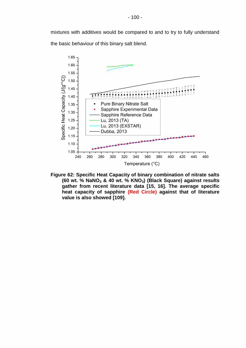
- 100 -

mixtures with additives would be compared to and to try to fully understand

the basic behaviour of this binary salt blend.

Figure 62: Specific Heat Capacity of binary combination of nitrate salts (60 wt. % NaNO3 & 40 wt. % KNO3) (Black Square) against results gather from recent literature data [15, 16]. The average specific heat capacity of sapphire (Red Circle) against that of literature value is also showed [109].

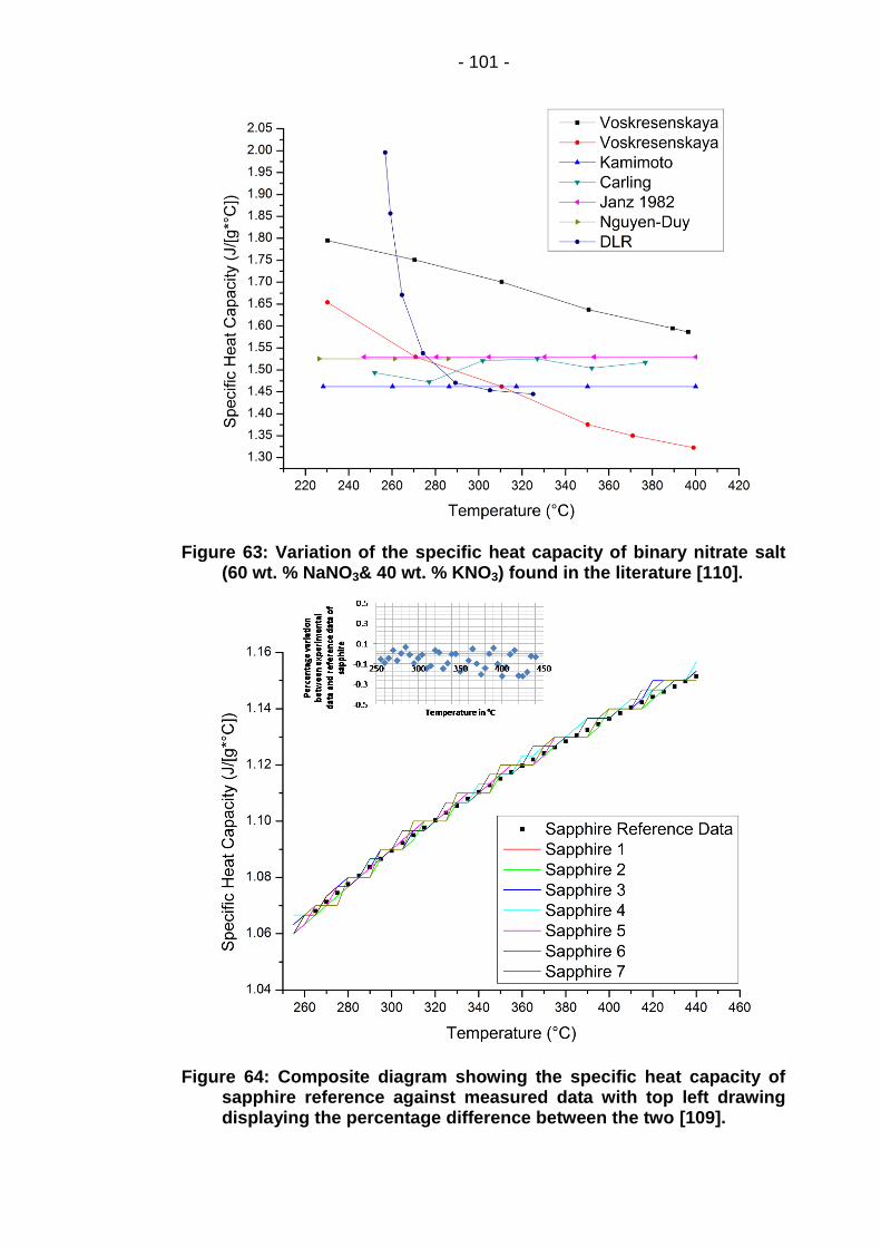
- 101 -

Figure 63: Variation of the specific heat capacity of binary nitrate salt (60 wt. % NaNO3& 40 wt. % KNO3) found in the literature [110].

Figure 64: Composite diagram showing the specific heat capacity of sapphire reference against measured data with top left drawing displaying the percentage difference between the two [109].

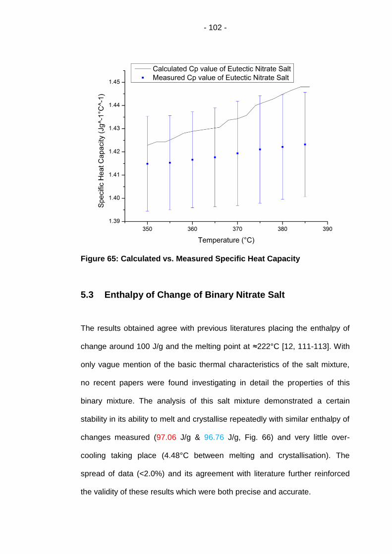
- 102 -

Figure 65: Calculated vs. Measured Specific Heat Capacity

5.3 Enthalpy of Change of Binary Nitrate Salt

The results obtained agree with previous literatures placing the enthalpy of

change around 100 J/g and the melting point at ≈222°C [12, 111-113]. With

only vague mention of the basic thermal characteristics of the salt mixture,

no recent papers were found investigating in detail the properties of this

binary mixture. The analysis of this salt mixture demonstrated a certain

stability in its ability to melt and crystallise repeatedly with similar enthalpy of

changes measured (97.06 J/g & 96.76 J/g, Fig. 66) and very little over-

cooling taking place (4.48°C between melting and crystallisation). The

spread of data (<2.0%) and its agreement with literature further reinforced

the validity of these results which were both precise and accurate.

- 103 -

Figure 66: Melting and crystallisation of binary nitrate salts (60 wt. % NaNO3 & 40 wt. % KNO3). Table within the graph shows the mean value of the 18 tests carried out.

5.4 Thermo-Gravimetric Analysis of Binary Nitrate Salt

The decomposition of this nitrate salt mixture showed that it was stable up to

550°C. Above that point, there was rapid degradation (75% mass loss, Fig.

67) of the salt, with most of the mass, lost between 550°C and 800°C.

Gradual settling of the weight occurred above 800°C implying that a solid

stable compound was produced. With a nitrogen atmosphere used to

prevent oxidation, most of the mass loss will have been through the release

of nitrogen and oxygen gas. The solid mass left in the crucible will probably

be a blend of potassium and sodium oxide.

- 104 -

The chemical transitions occurring during the decomposition of this salt will

be the following [114]:

NaNO3 (l) ↔ NaNO2 (l) + 1/2O2 (g) This pseudo-equilibrium occurred

above 550°C

2NaNO2 (l) → Na2O(s) + N2 (g) + 3/2O2(g) As temperature rose, the nitrite

further decomposed producing nitrogen gas and sodium oxide.

In a similar manner to NaNO3, KNO3(l) ↔ KNO2 (l) + 1/2O2 (g) goes into a

pseudo-equilibrium above 550°C

2KNO2 (l) → K2O + N2 + 3/2O2 (g) Decomposition led to the production of

oxides which explained why the mass settled at 25%, as a blend of

both potassium and sodium oxide were produced.

The flow of nitrogen through the furnace would have pushed the equilibrium

toward the production of nitrite by removing any gas created.

Figure 67: Thermo-gravimetric analysis of binary nitrate mixtures (60 wt. % NaNO3 & 40 wt. % KNO3) where percentage mass loss (left x-axis) and heat flow (right x-axis) are plotted against temperature.

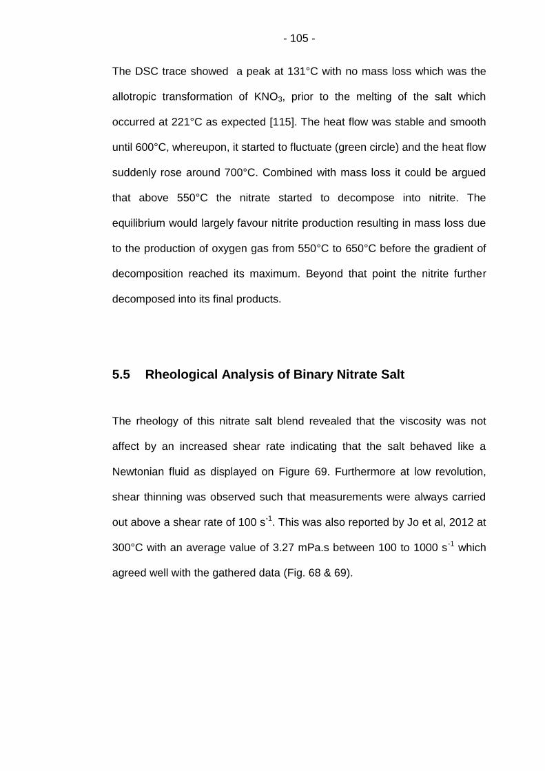
- 105 -

The DSC trace showed a peak at 131°C with no mass loss which was the

allotropic transformation of KNO3, prior to the melting of the salt which

occurred at 221°C as expected [115]. The heat flow was stable and smooth

until 600°C, whereupon, it started to fluctuate (green circle) and the heat flow

suddenly rose around 700°C. Combined with mass loss it could be argued

that above 550°C the nitrate started to decompose into nitrite. The

equilibrium would largely favour nitrite production resulting in mass loss due

to the production of oxygen gas from 550°C to 650°C before the gradient of

decomposition reached its maximum. Beyond that point the nitrite further

decomposed into its final products.

5.5 Rheological Analysis of Binary Nitrate Salt

The rheology of this nitrate salt blend revealed that the viscosity was not

affect by an increased shear rate indicating that the salt behaved like a

Newtonian fluid as displayed on Figure 69. Furthermore at low revolution,

shear thinning was observed such that measurements were always carried

out above a shear rate of 100 s-1. This was also reported by Jo et al, 2012 at

300°C with an average value of 3.27 mPa.s between 100 to 1000 s-1 which

agreed well with the gathered data (Fig. 68 & 69).

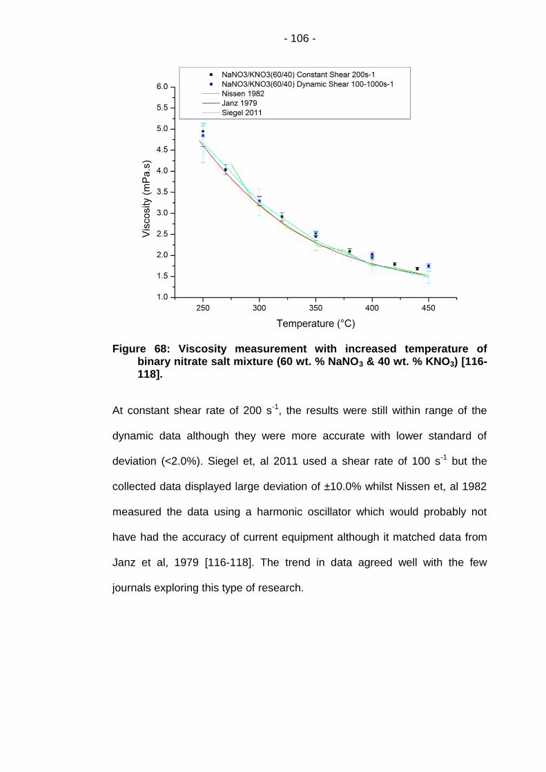
- 106 -

Figure 68: Viscosity measurement with increased temperature of binary nitrate salt mixture (60 wt. % NaNO3 & 40 wt. % KNO3) [116-118].

At constant shear rate of 200 s-1, the results were still within range of the

dynamic data although they were more accurate with lower standard of

deviation (<2.0%). Siegel et, al 2011 used a shear rate of 100 s-1 but the

collected data displayed large deviation of ±10.0% whilst Nissen et, al 1982

measured the data using a harmonic oscillator which would probably not

have had the accuracy of current equipment although it matched data from

Janz et al, 1979 [116-118]. The trend in data agreed well with the few

journals exploring this type of research.

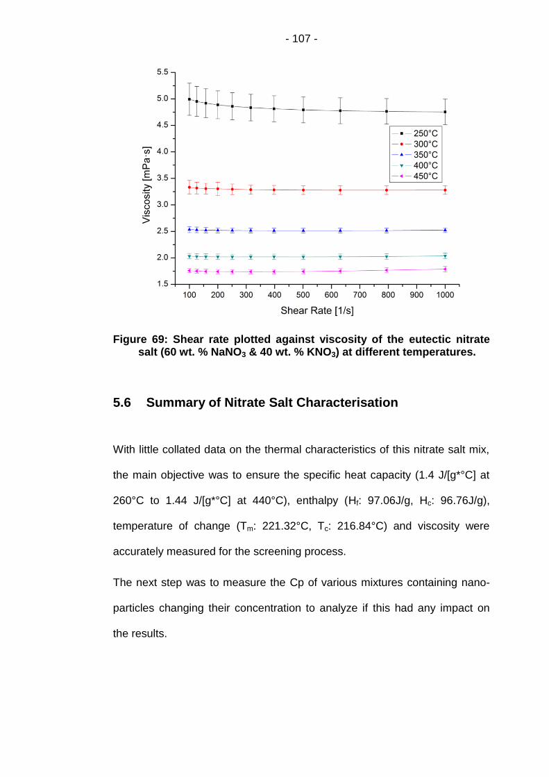
- 107 -

Figure 69: Shear rate plotted against viscosity of the eutectic nitrate salt (60 wt. % NaNO3 & 40 wt. % KNO3) at different temperatures.

5.6 Summary of Nitrate Salt Characterisation

With little collated data on the thermal characteristics of this nitrate salt mix,

the main objective was to ensure the specific heat capacity (1.4 J/[g*°C] at

260°C to 1.44 J/[g*°C] at 440°C), enthalpy (Hf: 97.06J/g, Hc: 96.76J/g),

temperature of change (Tm: 221.32°C, Tc: 216.84°C) and viscosity were

accurately measured for the screening process.

The next step was to measure the Cp of various mixtures containing nano-

particles changing their concentration to analyze if this had any impact on

the results.

- 108 -

Chapter 6 Results & Discussion: Salt Characterisation with

Additives

This chapter discuss the results obtained in the screening process of nano-

particle additives in eutectic mixture of nitrates (60 wt% NaNO3 & 40 wt%

KNO3).

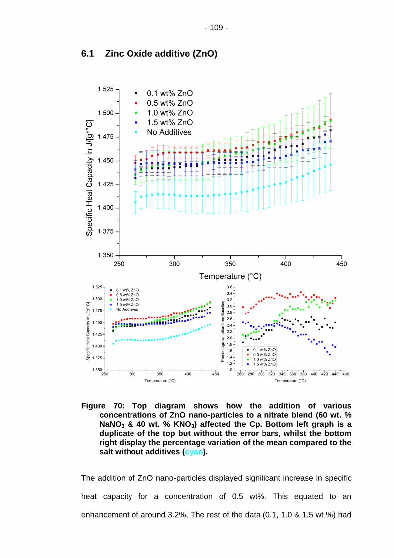
- 109 -

6.1 Zinc Oxide additive (ZnO)

Figure 70: Top diagram shows how the addition of various concentrations of ZnO nano-particles to a nitrate blend (60 wt. % NaNO3 & 40 wt. % KNO3) affected the Cp. Bottom left graph is a duplicate of the top but without the error bars, whilst the bottom right display the percentage variation of the mean compared to the salt without additives (cyan).

The addition of ZnO nano-particles displayed significant increase in specific

heat capacity for a concentration of 0.5 wt%. This equated to an

enhancement of around 3.2%. The rest of the data (0.1, 1.0 & 1.5 wt %) had

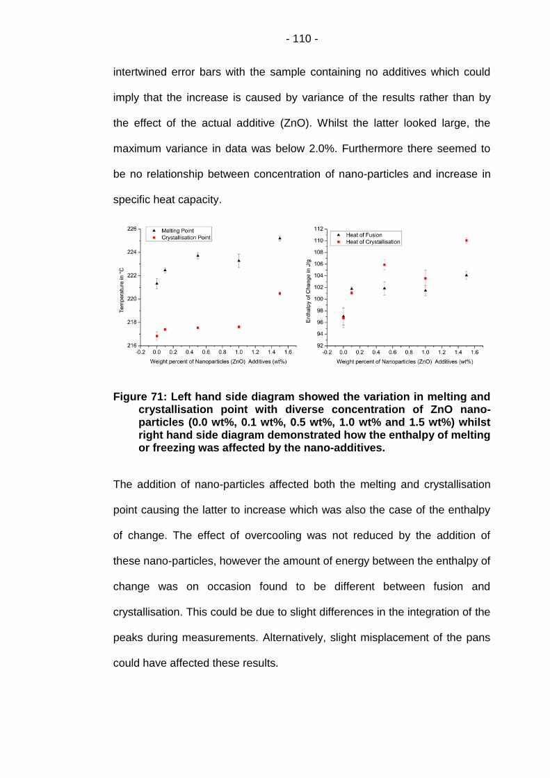
- 110 -

intertwined error bars with the sample containing no additives which could

imply that the increase is caused by variance of the results rather than by

the effect of the actual additive (ZnO). Whilst the latter looked large, the

maximum variance in data was below 2.0%. Furthermore there seemed to

be no relationship between concentration of nano-particles and increase in

specific heat capacity.

Figure 71: Left hand side diagram showed the variation in melting and crystallisation point with diverse concentration of ZnO nano-particles (0.0 wt%, 0.1 wt%, 0.5 wt%, 1.0 wt% and 1.5 wt%) whilst right hand side diagram demonstrated how the enthalpy of melting or freezing was affected by the nano-additives.

The addition of nano-particles affected both the melting and crystallisation

point causing the latter to increase which was also the case of the enthalpy

of change. The effect of overcooling was not reduced by the addition of

these nano-particles, however the amount of energy between the enthalpy of

change was on occasion found to be different between fusion and

crystallisation. This could be due to slight differences in the integration of the

peaks during measurements. Alternatively, slight misplacement of the pans

could have affected these results.

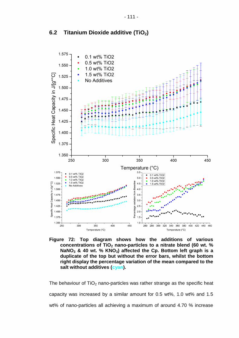
- 111 -

6.2 Titanium Dioxide additive (TiO2)

Figure 72: Top diagram shows how the additions of various concentrations of TiO2 nano-particles to a nitrate blend (60 wt. % NaNO3 & 40 wt. % KNO3) affected the Cp. Bottom left graph is a duplicate of the top but without the error bars, whilst the bottom right display the percentage variation of the mean compared to the salt without additives (cyan).

The behaviour of TiO2 nano-particles was rather strange as the specific heat

capacity was increased by a similar amount for 0.5 wt%, 1.0 wt% and 1.5

wt% of nano-particles all achieving a maximum of around 4.70 % increase

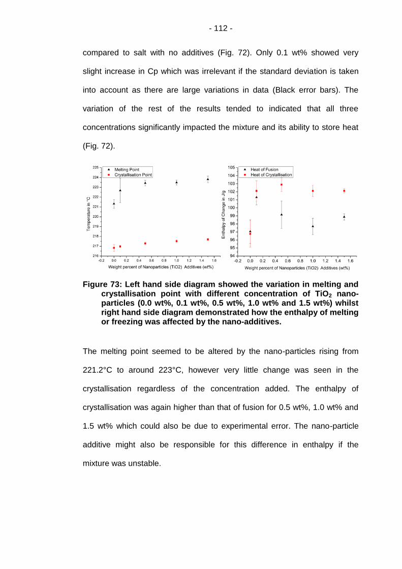
- 112 -

compared to salt with no additives (Fig. 72). Only 0.1 wt% showed very

slight increase in Cp which was irrelevant if the standard deviation is taken

into account as there are large variations in data (Black error bars). The

variation of the rest of the results tended to indicated that all three

concentrations significantly impacted the mixture and its ability to store heat

(Fig. 72).

Figure 73: Left hand side diagram showed the variation in melting and crystallisation point with different concentration of TiO2 nano-particles (0.0 wt%, 0.1 wt%, 0.5 wt%, 1.0 wt% and 1.5 wt%) whilst right hand side diagram demonstrated how the enthalpy of melting or freezing was affected by the nano-additives.

The melting point seemed to be altered by the nano-particles rising from

221.2°C to around 223°C, however very little change was seen in the

crystallisation regardless of the concentration added. The enthalpy of

crystallisation was again higher than that of fusion for 0.5 wt%, 1.0 wt% and

1.5 wt% which could also be due to experimental error. The nano-particle

additive might also be responsible for this difference in enthalpy if the

mixture was unstable.

- 113 -

6.3 Copper additive (Cu)

Figure 74: Top diagram shows how the additions of various concentrations of Cu nano-particles to a nitrate mix (60 wt. % NaNO3 & 40 wt. % KNO3) affected the Cp. Bottom left graph is a duplicate of the top but without the error bars, whilst the bottom right display the percentage variation of the mean compared to the salt without additives (cyan).

The utilization of copper nano-particles was interesting as the latter

appeared to be dependent on the concentration of additives present in the

blend. As the concentration of nano-particles decreased from 1.5 wt% to 0.1

- 114 -

wt%, the maximum mean percentage variation rose from 1.0 % to 3.6 %

(Fig. 74). In term of the significance of the results both 1.0 wt% and 1.5 wt%

had intertwined error bars with the pure salt (no additives) which would imply

that the obtained increase could potentially be due to error. This is not the

case for 0.1 wt% and 0.5 wt%.

Figure 75: Left hand side diagram showed the variation in melting and crystallisation point with varied concentration of Cu nano-particles (0.0 wt%, 0.1 wt%, 0.5 wt%, 1.0 wt% and 1.5 wt%) whilst right hand side diagram demonstrated how the enthalpy of melting or freezing was affected by the nano-additives.

As described before the melting point slightly increase with 0.1 wt% Cu and

then gradually decrease from 0.5 wt% to 1.5 wt% to reach a value similar to

that of the pure binary mixture. The crystallisation temperature was however

similar with little variance seen. As for the enthalpy of fusion, there also

seemed to be very little variation in between the different concentration of

nano-particles utilized but the overall trend was an increase in thermal

energy needed to melt the sample, although that increase was slight.

- 115 -

6.4 Silicon dioxide additive (SiO2)

Figure 76: Top diagram shows how the additions of various concentrations of SiO2 nano-particles to a nitrate blend (60 wt. % NaNO3 & 40 wt. % KNO3) affected the Cp. Bottom left graph is a duplicate of the top but without the error bars, whilst the bottom right display the percentage variation of the mean compared to the salt without additives (cyan).

The results gathered for the use of silicon dioxide nano-particles displayed a

maximum increase of around 4.0 % for 1.5 wt% and 0.5 wt% additives.

However the large variation in the obtained data could indicate that the

- 116 -

mixture was unstable which could also explain the negative enhancement

seen for 1.0 wt %. There seemed to be no clear relationship between

percentage additive and Cp change.

Figure 77: Left hand side diagram showed the variation in melting and crystallisation point with varied concentration of SiO2 nano-particles (0.0 wt%, 0.1 wt%, 0.5 wt%, 1.0 wt% and 1.5 wt%) whilst right hand side diagram demonstrated how the enthalpy of melting or freezing was affected by the nano-additives.

Both melting and crystallisation point as well as enthalpy of change were

higher for the mixture containing SiO2.

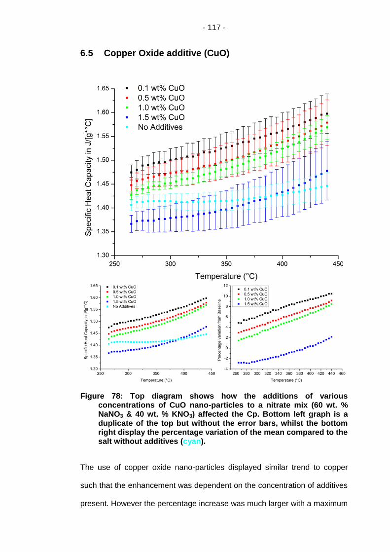
- 117 -

6.5 Copper Oxide additive (CuO)

Figure 78: Top diagram shows how the additions of various concentrations of CuO nano-particles to a nitrate mix (60 wt. % NaNO3 & 40 wt. % KNO3) affected the Cp. Bottom left graph is a duplicate of the top but without the error bars, whilst the bottom right display the percentage variation of the mean compared to the salt without additives (cyan).

The use of copper oxide nano-particles displayed similar trend to copper

such that the enhancement was dependent on the concentration of additives

present. However the percentage increase was much larger with a maximum

- 118 -

increase of 10.5 % with 0.1 wt% CuO, 9.2 % with 0.5 wt % CuO and finally

8.5 % with 1.0 wt % CuO. The use of 1.5 wt % CuO caused a large

decrease in the Cp and the maximum end up been 2.1 %. The variation of

the data (<3.0%) clearly demonstrated no intertwined error bar for the first

three concentrations, which validated the beneficial effect of this particular

additives.

Figure 79: Left hand side diagram showed the variation in melting and crystallisation point with diverse concentration of CuO nano-particles (0.0 wt%, 0.1 wt%, 0.5 wt%, 1.0 wt% and 1.5 wt%) whilst right hand side diagram demonstrated how the enthalpy of melting or freezing was affected by the nano-additives.

The melting point was increased with 0.1 wt % and 1.5 wt % of CuO whilst

the crystallisation point showed only slight increase for 1.5 wt%. The

enthalpy values were the same for both crystallisation and fusion which was

to be expected except that of 0.1 wt % CuO which displayed differing values.

- 119 -

6.6 Summary & Further Discussion

6.6.1 Summary

The aim of this screening process was to investigate how the addition of

various nano-particles affected a eutectic mixture of nitrate (60 wt% NaNO3

& 40 wt% KNO3) and which concentration resulted in the highest Cp

enhancement.

The results demonstrated that the addition of nano-particles had in most

cases a beneficiary effect toward the specific heat capacity (Table 6). This

was unlike published data by Chieruzzi, et al, 2013 which displayed negative

enhancement when using TiO2 and SiO2 nano-particles (0.5, 1.0 & 1.5 wt.%)

[119]. Dubba, et al, 2013 on the other hand displayed positive enhancement

of SiO2 of 10% to 28% depending on the size of the nano-particles. Of the

screening process, 0.1 wt% copper oxide displayed the largest increase

(Table 6).

The melting and crystallisation point as well as the enthalpy of change

(fusion/solidification) tended to increase whilst the actual onset of melting

decrease similarly to what is stated by Chieruzzi, et al, 2013 [119] (Table 7).

Whilst this may seem contradictory, the change of phase is defined by three

stages. The onset of melting is interpreted as the temperature at which the

sample started to collapse on itself such that the salt started to adhere to the

side of the platinum crucible. At this point in time a semi-liquid phase is

created whereupon not all of the salt is at liquid state. The melting point was

therefore defined as the high temperature at which the salt was fully melted.

- 120 -

Table 6: Mean percentage enhancement of Cp at 440°C for different type and concentration of nano-particles

Nano-particles concentration

wt.%

Specific Heat Capacity in

J/[g°C] in liquid phase at 440°C

Percentage Enhancement at

440°C

Base Salt 0 1.446 -

Base Salt + ZnO

0.1 1.482 2.49

0.5 1.493 3.26

1 1.492 3.18

1.5 1.471 1.72

Base Salt + TiO2

0.1 1.468 1.57

0.5 1.517 4.95

1 1.514 4.72

1.5 1.516 4.84

Base Salt + Cu

0.1 1.498 3.64

0.5 1.484 2.64

1 1.463 1.18

1.5 1.462 1.10

Base Salt + SiO2

0.1 1.487 2.87

0.5 1.507 4.26

1 1.440 -0.42

1.5 1.503 3.95

Base Salt + CuO

0.1 1.597 10.48

0.5 1.578 9.17

1 1.568 8.48

1.5 1.477 2.18

In theory the melting range of a pure sample is very low and only spanned

for a couple of degrees Celsius. In this case, however the salt without

additive was already a binary mixture of salt (NaNO3 = Tm 308.01°C + KNO3

= Tm 336.03°C with ratio 60/40) which increase the entropy thereby lowering

the melting point to 221.32°C. Through the same train of thought, any nano-

particles addition to the binary salt mixture can be regarded as impurities

increasing furthermore the level of entropy. This should in theory lead to a

lower onset of melting and a broader peak during the melting process.

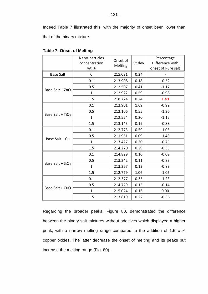
- 121 -

Indeed Table 7 illustrated this, with the majority of onset been lower than

that of the binary mixture.

Table 7: Onset of Melting

Nano-particles concentration

wt.%

Onset of Melting

St.dev Percentage

Difference with onset of Pure salt

Base Salt 0 215.031 0.34 -

Base Salt + ZnO

0.1 213.908 0.18 -0.52

0.5 212.507 0.41 -1.17

1 212.922 0.59 -0.98

1.5 218.224 0.24 1.49

Base Salt + TiO2

0.1 212.901 1.69 -0.99

0.5 212.106 0.55 -1.36

1 212.554 0.20 -1.15

1.5 213.143 0.19 -0.88

Base Salt + Cu

0.1 212.773 0.59 -1.05

0.5 211.951 0.09 -1.43

1 213.427 0.20 -0.75

1.5 214.270 0.29 -0.35

Base Salt + SiO2

0.1 214.829 0.10 -0.09

0.5 213.242 0.11 -0.83

1 213.257 0.12 -0.83

1.5 212.779 1.06 -1.05

Base Salt + CuO

0.1 212.377 0.35 -1.23

0.5 214.729 0.15 -0.14

1 215.024 0.16 0.00

1.5 213.819 0.22 -0.56

Regarding the broader peaks, Figure 80, demonstrated the difference

between the binary salt mixtures without additives which displayed a higher

peak, with a narrow melting range compared to the addition of 1.5 wt%

copper oxides. The latter decrease the onset of melting and its peaks but

increase the melting range (Fig. 80).

- 122 -

Figure 80: Illustration of the difference in shape and size of the peaks when nano-particle (1.5 wt% CuO) was present or absent.

6.6.2 Discussion

The addition of nano-particles to ionic fluids such as inorganic salt clearly

affected the thermo-physical characteristics of the fluid. The presence of

nano-sized solid particles will influence both the thermal conductivity and

specific heat capacity of the molten salt. With large surface area to volume

ratio, the nano-particle will display thermo-physical properties different from

bulk. It is known that nano-particles display higher surface energy compared

to bulk [91]. This is due to an increased degree of freedom in atoms found

at the edges of nano-particles which display lower vibrational energy

compared to atoms located away from the edges. As heat capacity is linked

to the structure of the nano-particle, its vibrational and configurational

entropy, decreasing the size of nano-particles is going to lead to a rise in the

- 123 -

amount of exposed atoms. Whilst this has been showed to promote an

increase in specific heat capacity, many factors such as shape, purity and

density to name but a few might also affect this thermal properties [92].

Described as a potential mode for the enhancement of Cp in Chapter 2.8, it

is unlikely to be one of the main mechanism that could explain this abnormal

rise. With values below that of molten salt, the increase in Cp cannot be

explained by this mode alone as this solid structure would have to display

extremely high Cp to cause a 10.0% rise with a 0.1 weight percent fraction of

CuO added. Furthermore theoretical description of Cp through the Einstein

or Debye heat capacity model demonstrate that a plateau is reached at high

temperature whereupon the value does no increase and stays constant.

Whilst Einstein model assumes a single vibration frequency in solid, Debye

regards it as a continuous elastic solid meaning that the calculation of

temperature in each model differs [120]. However at high temperature, the

correlation of both model is similar.

Figure 81: Schematic of heat capacity of Bulk material vs. Nano-particle on the left and on the right a representation of a solid lattice of atoms where the vibrational energy between atoms is responsible for the heat capacity storage.

- 124 -

Stored through vibrational frequency between atoms, the latter is directly

correlated to temperature. At zero degree Kelvin no energy can theoretically

be stored. As temperature increase, frequency of vibration between atoms

increase up to a point where maximum value is reached.

The next potential mode of energy storage was identified to be the interfacial

resistance (Mode 2: Chapter 2.8, Fig. 82) taking place between the solid and

liquid. Indeed at this point, the transfer of energy is disrupted due to a

change in electronic and vibrational properties as energy carrier such as

phonon or electron try to cross this boundary. It is unlikely that this Mode is

responsible for specific heat capacity although it might play a role in the

enhancement of Cp by providing storage through the difference in vibrational

energy between that of the solid nano-particle and the liquid layer.

Furthermore the liquid present at this boundary is constrained, displaying a

semi-solid behaviour as the atoms surrounding the nano-particle are packed

forming a layered interface (Mode 3: Chapter 2.8, Fig. 82). Oh et al, 2005

showed that liquid aluminium atoms formed a layered structure at the

interface with alumina [98].

Figure 82: Schematic diagram of Mode II & III

- 125 -

Similarly it has long been identified that these compressed liquid layers

might play an important role in the thermal conductivity as the layered atoms

around the nano-particle display properties akin to that of solid [121-123].

To account for the increase in specific heat capacity, one would have to

postulate that the property of these compressed layers are higher than that

of bulk solid by partially accounting for the enthalpy of fusion as these layers

would be located in between two phases (Semi-Solid) due to the loosely

packed atoms [124]. Therefore the calculation of specific heat capacity

needs to take into account the mass fraction of nano-particles as well as the

specific heat capacity of the compressed liquid layers.

Following on the same train of thought, the volume of compressed liquid

layers will be influenced by the shape and size of the nano-particles. As

surface area of contact seems to be of importance, a small tetrahedron

nano-particle (10 nm in size) should provide higher increase in Cp compared

to a spherical structure of the same dimension. Similarly, decreasing the size

will enhance the available surface area of contact.

However agglomeration will negatively impact enhancement by reducing the

total volume. This will be dependent of the methodology of dispersion used

as it might affect surface properties of the nano-particle and how they

interact.

- 126 -

6.7 Powder vs. Liquid Dispersion

Unlike low temperature fluid, where the use of surfactant and alteration of pH

are common variables changed to increase the stability of the suspension

over time, nano-particles dispersion into inorganic salt cannot be easily

modified once introduced in its liquid phase. This implied that dispersion has

to be done before melting ever occurred. Two methods of dispersions were

thought of:

Liquid dispersion where the salt is dissolved into distilled water and

the nano-particles added. This was followed by sonication,

evaporation and removal of hydrates through melting of sample

(>250°C). This method of dispersion has been widely used in several

research papers [14-16, 90, 119]. One of the first published paper

displaying this method was Shin & Banerjee, 2011 [90].

Powder dispersion entailed the use of a mill to grind and mix the salt

and nano-particles together. This technique was used for all of the

previously showed specific heat capacity work.

Here it was demonstrated that regardless of the method used the specific

heat capacity was almost the same (Fig. 84). This was good news, as the

scalability of the powder dispersion was more practical and economically

viable compare to the liquid method.

Further characterisation into the method of production showed that the

melting, crystallisation and enthalpy of change were significantly increased

when the liquid dispersion method was used compared to the milling method

(Fig. 85).

- 127 -

Figure 83: Variation in Cp depending on the method used to produce the sample. The bracketed Banerjee name referred to the liquid dispersion whilst the other (Green) was mixed using powder dispersion.

The liquid method displayed the advantage, through sonication, of allowing

the homogenous dispersion of the nano-particles and promoted any

aggregates that might have formed to be broken through this process.

However the evaporation of water and eventual re-crystallisation might on

the contrary lead to the formation of aggregate as the volume of water

dropped and the salt crystal formed.

The physical method on the other hand would cause the nano-particles to

adhere on the salt surface. The grinding of the potassium and sodium nitrate

prior to the introduction of nano-particles would increase the surface area

allowing a greater spread of the latter. The only downsides of this method

- 128 -

would be the loss of a fraction of nano-particles that adhered to the ball

bearing used as well as the potential contamination.

Figure 84: Effect of different dispersion method on the melting/crystallisation and enthalpy of change of 1.0 wt% CuO additives compared to binary nitrate salt (60 wt. % NaNO3 & 40 wt. % KNO3)

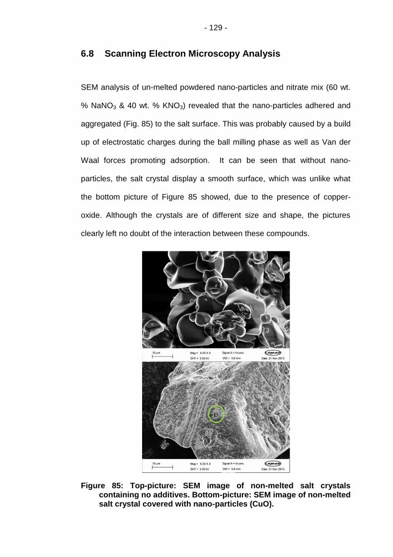
- 129 -

6.8 Scanning Electron Microscopy Analysis

SEM analysis of un-melted powdered nano-particles and nitrate mix (60 wt.

% NaNO3 & 40 wt. % KNO3) revealed that the nano-particles adhered and

aggregated (Fig. 85) to the salt surface. This was probably caused by a build

up of electrostatic charges during the ball milling phase as well as Van der

Waal forces promoting adsorption. It can be seen that without nano-

particles, the salt crystal display a smooth surface, which was unlike what

the bottom picture of Figure 85 showed, due to the presence of copper-

oxide. Although the crystals are of different size and shape, the pictures

clearly left no doubt of the interaction between these compounds.

Figure 85: Top-picture: SEM image of non-melted salt crystals containing no additives. Bottom-picture: SEM image of non-melted salt crystal covered with nano-particles (CuO).

- 130 -

Figure 86: Scaled up version the bottom picture in Figure 99 (green circle showed the area focused on).

The nano-particles visibly altered the crystal formation of the binary nitrate

mixture (Fig. 87 & 88). As written previously, the formation of ‘nano-

structures’ stated in Dubba et, al. 2013 and Tiznobaik & Shin. 2013 could be

due to the formation of semi-solid layers around the nano-particles [15, 93].

Due to their large surface area to volume ratio, the behaviour of nano-

particles differ substantially from bulk and papers have showed that

increasing this ratio led to a blue shift in infrared spectroscopy due to the rise

in the amount of exposed surface atoms [91, 92]. Whilst the nano-particles

itself would not cause the enhancement of specific heat capacity, its

interaction with molten salt liquid and particularly the formation of nano-

layers might be the main mechanism responsible for this rise.

- 131 -

Figure 87: Melted binary nitrate mixture (60 wt. % NaNO3& 40 wt. % KNO3) containing no nano-particle additive.

Figure 88: Melted binary nitrate mixture (60 wt. % NaNO3& 40 wt. % KNO3) containing varied concentration of CuO nano-particle additive (A = 0.1 wt% CuO, B = 0.5 wt% CuO, C = 1.0 wt% CuO & D = 1.5 wt% CuO)

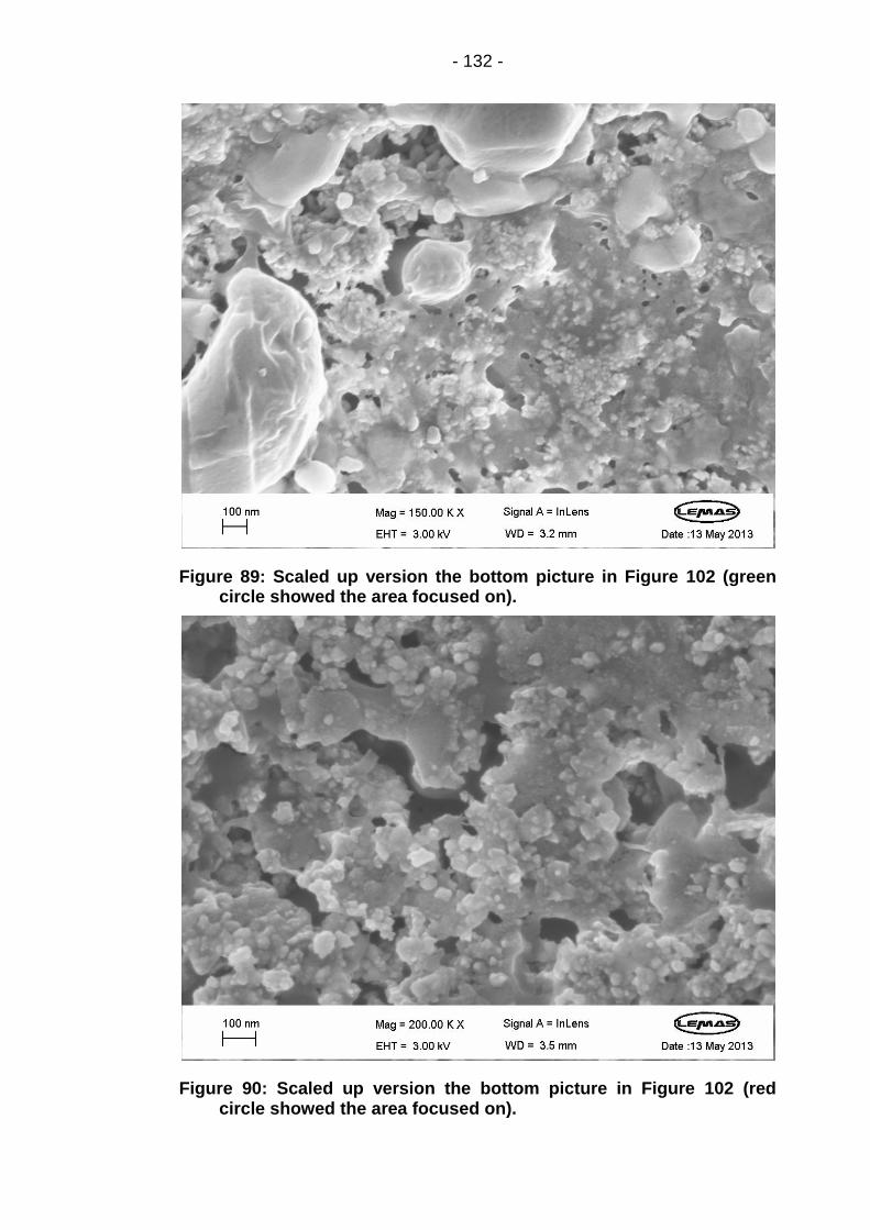
- 132 -

Figure 89: Scaled up version the bottom picture in Figure 102 (green circle showed the area focused on).

Figure 90: Scaled up version the bottom picture in Figure 102 (red circle showed the area focused on).

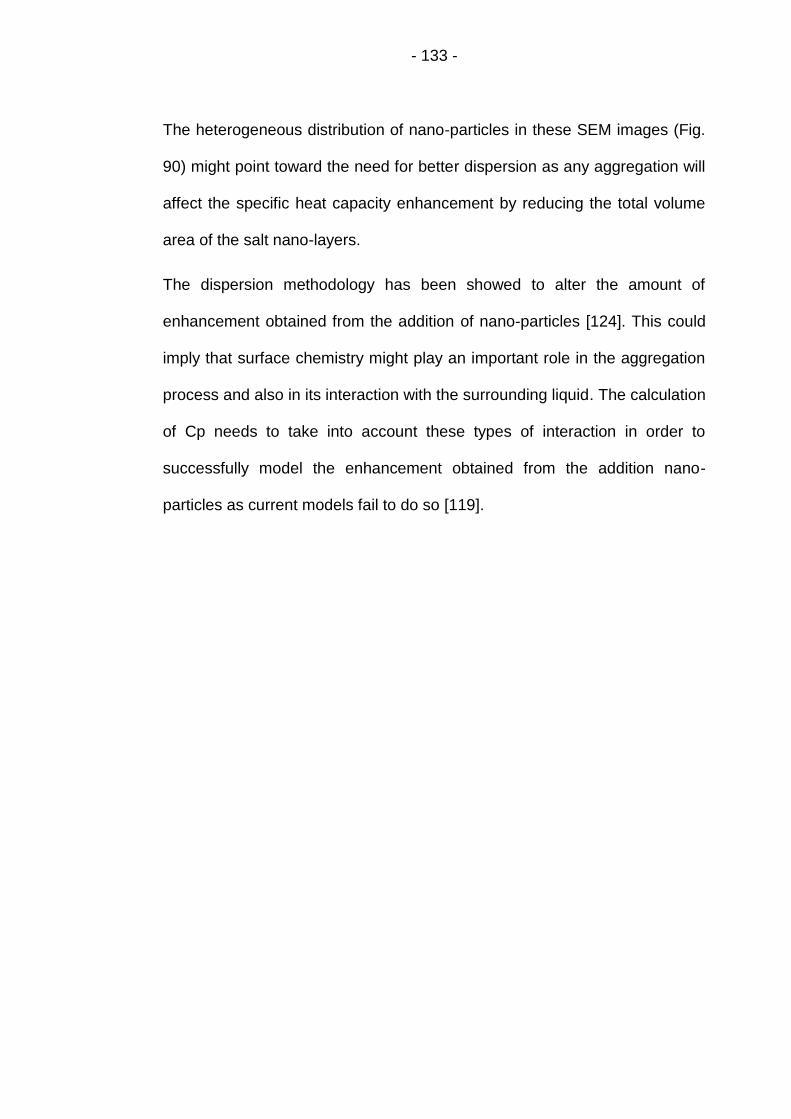
- 133 -

The heterogeneous distribution of nano-particles in these SEM images (Fig.

90) might point toward the need for better dispersion as any aggregation will

affect the specific heat capacity enhancement by reducing the total volume

area of the salt nano-layers.

The dispersion methodology has been showed to alter the amount of

enhancement obtained from the addition of nano-particles [124]. This could

imply that surface chemistry might play an important role in the aggregation

process and also in its interaction with the surrounding liquid. The calculation

of Cp needs to take into account these types of interaction in order to

successfully model the enhancement obtained from the addition nano-

particles as current models fail to do so [119].

- 134 -

6.9 Rheological Analysis of 0.1 wt% CuO additives

Figure 91: Viscosity profile of binary nitrate mixture (60 wt. % NaNO3 & 40 wt. % KNO3) containing 0.1 wt% Copper Oxide against increasing shear rate.

The use of 0.1 wt% Copper oxide nano-particles in the binary salt displayed

a Newtonian fluid behaviour above 100 s-1 as it was expected. The mean

viscosity increased with temperature when the additive was present which

agreed with data obtained Jo et al. 2012 who tested the viscosity of a binary

nitrate composition with and without 1.0 wt% SiO2 and found an increase at

300°C and 400°C of 63% and 79% respectively [125].

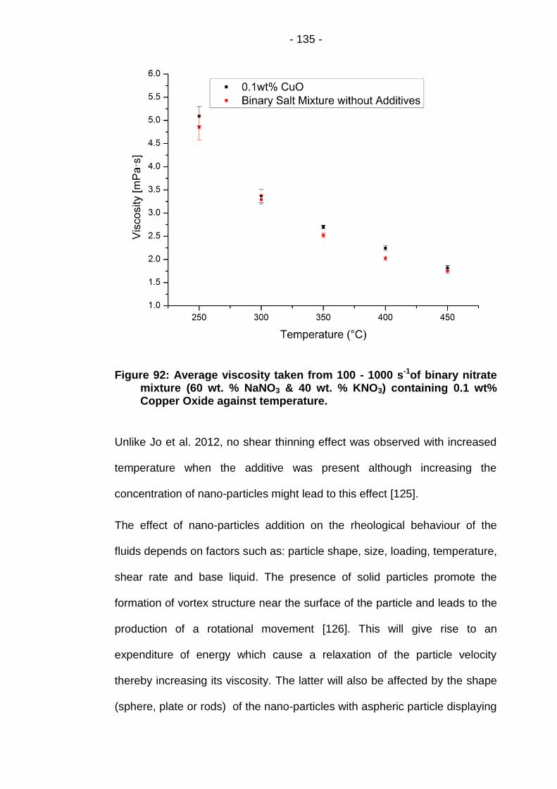
- 135 -

Figure 92: Average viscosity taken from 100 - 1000 s-1of binary nitrate mixture (60 wt. % NaNO3 & 40 wt. % KNO3) containing 0.1 wt% Copper Oxide against temperature.

Unlike Jo et al. 2012, no shear thinning effect was observed with increased

temperature when the additive was present although increasing the

concentration of nano-particles might lead to this effect [125].

The effect of nano-particles addition on the rheological behaviour of the

fluids depends on factors such as: particle shape, size, loading, temperature,

shear rate and base liquid. The presence of solid particles promote the

formation of vortex structure near the surface of the particle and leads to the

production of a rotational movement [126]. This will give rise to an

expenditure of energy which cause a relaxation of the particle velocity

thereby increasing its viscosity. The latter will also be affected by the shape

(sphere, plate or rods) of the nano-particles with aspheric particle displaying

- 136 -

much higher viscosity than their spherical counterpart at the same

concentration [127]. Furthermore the shear rate used to perform the tests

will affect particle-particle interaction as the latter will grow weaker and brake

down with rising shear rate leading to shear thinning. At constant shear, it is

of general consensus among literatures that, as the particle concentration

increases, the viscosity of the fluid rises [128]. The percentage enhancement

of viscosity is still dependent on factors such as shape, size, temperature,

base fluid and shear used.

In the experimental setup, the base fluid, molten salt, demonstrated a

Newtonian behaviour between 100 s-1 and 1000 s-1. At these rotational

speed and with the low concentration of nano-particles present, it is not

surprising to see a Newtonian behaviour as the fast rotational force applied

on the fluid would lead to dispersion of nano-particles breaking the formation

of aggregate if any were present to begin with. The use of a larger

concentration of nano-particle (1.0 to 5.0 wt.%) and a low shear rate to begin

with 1.0 s-1 might cause the formation of aggregate leading to a rise in

viscosity slowly decreasing with increased shear force.

Figure 93: Effect of shear rate on viscosity [126, 127, 129]

- 137 -

These perturbations in fluid flow are considered by the Einstein’s theory

formulated in 1906, for spherical particles with low volume fraction. With

many systems and experimental setup produced, different mathematical

models have been created trying to fit the obtained data with theoretical

values [128, 130].

- 138 -

6.10 Further Discussion & Summary

Understanding the effect of nano-particles in molten salt is important in the

development of stable nano-fluid formulation capable of storing and

transferring large quantities of thermal energy. Flowing through a circular

piping system, the molten salt would display a turbulent behaviour. The latter

would allow for a better more efficient transfer of heat within the system due

to the production of ‘eddies’. The type of heat transfer can be calculated

through the Prandtl number (Pr).

Written as;

Pr = µCp / k

where µ is the dynamic viscosity (N.s.m-2), Cp is the specific heat capacity

(J/[g*K]) and k is the thermal conductivity (W/[m*K]). This equation evaluate

which mode of energy transfer is dominant. It follows that, Pr > 1 imply that

the main mode of heat transfer is dictated by convection whilst Pr < 1 means

that thermal conduction dominates. Using Dittus Boelter equation to model a

simple turbulent flow inside circular pipe, the heat transfer coefficient can be

derived from the following equation where:

Nu = 0.023 Re0.8 * Pr1/3

hd/k = 0.023 (jd/µ)0.8 * (µCp/k)1/3

h = Heat transfer coefficient (W/[m2*K])

d = Diameter of pipe (m)

k = Thermal conductivity (W/[m*K])

j = Mass flux (kg/[s*m-2])

- 139 -

µ = Viscosity ([N*s]/m2)

Cp = Specific heat capacity (J/[g*K])

Rearranging in term of heat transfer coefficient:

h = 0.023 [ j0.8 * Cp1/3 * k2/3 * µ-0.47 * d-0.2 ]

It can be seen from the above equation that enhancing the specific heat

capacity and/or thermal conductivity would have a positive effect on the heat

transfer coefficient. However the addition of nano-particle would lead to

increase viscosity which would be damaging to the heat transfer coefficient

as would an increase in the diameter of the piping system.

Whilst much research is still needed to be done before this technology is

implemented, the interaction between nano-particles and molten salt fluid

cannot be denied and their effect on heat transfer coefficient is positive

[131]. This should lead to a lower cost of electricity production in

concentrated solar power plant allowing it to further compete against non-

renewable energy sources.

This research has highlighted that repeated basic characterisation of binary

nitrate salt mixture has not been carried out in the literature. Indeed basic

specific heat capacity varies hugely which is probably due to the equipment

and technique used as demonstrated in the preliminary results obtained in

Chapter 3. The theory behind the improvement seen when utilizing nano-

particles might be due to the formation of nano-layers as molten salt ions

‘coat’ their surface. The latter would also affect other thermal characteristic

such as onset & point of melting/crystallisation as well as rheological

measurements.

- 140 -

Chapter 7 Results & Discussion: Stability Rigs

This chapter looks at the effects of physical mixing on the thermal

characteristics of the liquid salt when tested with additives and without

additives to monitor how this affected the dispersion of 0.1 wt% Copper

Oxide.

- 141 -

7.1 Static Rig with Binary Nitrate Salt – No Additives –

Negative Control

Results obtained showed that there was a defined difference in Cp between

the sample produced in the lab and the salt taken from the rig. The latter

displayed higher values which could be caused by impurities found in the

container. Indeed the molten salt is corrosive by nature and would start to

attack the stainless steel. Whilst this may be a very slow process, it might

affect the data gathered as the salts produced in the lab were not in contact

with steel under liquid form.

Figure 94: Difference in specific heat capacity between sample produce in the lab and directly tested on the DSC compared to sample obtained from the rig after different length of time (Standard Deviation <2.0%).

Evaluation of the melting point and enthalpy of fusion between the two

revealed that both were substantially higher which would tend to confirm the

- 142 -

slight change in the composition of the salt. Whilst the actual melting point

and enthalpy of fusion remained the same over 800 hours, the reaction of

the binary salt mixture with the stainless steel container might have led to

this rise.

Figure 95: Difference in melting point and enthalpy of fusion between sample taken from the rig and salt produced in the lab for binary nitrate mixture containing no additives.

Figure 96: Photographs of samples removed from the rigs at different times.

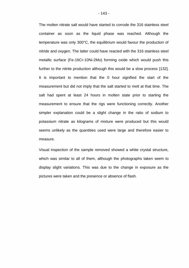
- 143 -

The molten nitrate salt would have started to corrode the 316 stainless steel

container as soon as the liquid phase was reached. Although the

temperature was only 300°C, the equilibrium would favour the production of

nitride and oxygen. The latter could have reacted with the 316 stainless steel

metallic surface (Fe-16Cr-10Ni-2Mo) forming oxide which would push this

further to the nitrite production although this would be a slow process [132].

It is important to mention that the 0 hour signified the start of the

measurement but did not imply that the salt started to melt at that time. The

salt had spent at least 24 hours in molten state prior to starting the

measurement to ensure that the rigs were functioning correctly. Another

simpler explanation could be a slight change in the ratio of sodium to

potassium nitrate as kilograms of mixture were produced but this would

seems unlikely as the quantities used were large and therefore easier to

measure.

Visual inspection of the sample removed showed a white crystal structure,

which was similar to all of them, although the photographs taken seem to

display slight variations. This was due to the change in exposure as the

pictures were taken and the presence or absence of flash.

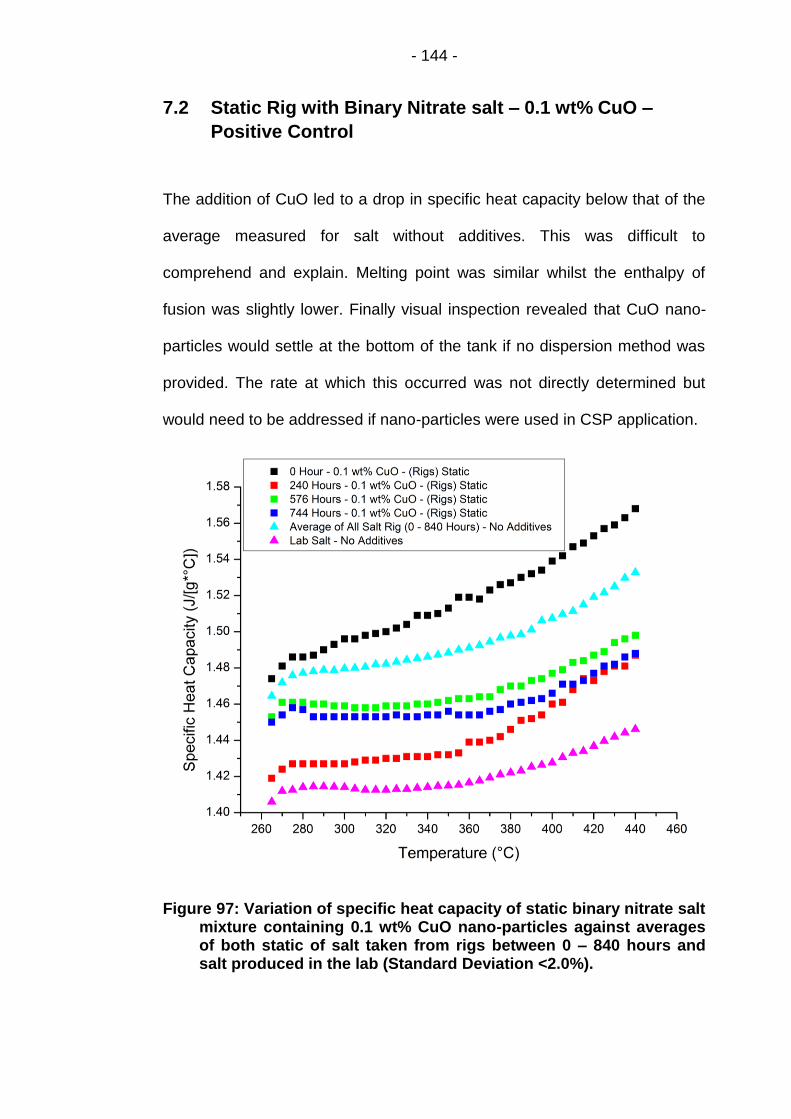
- 144 -

7.2 Static Rig with Binary Nitrate salt – 0.1 wt% CuO –

Positive Control

The addition of CuO led to a drop in specific heat capacity below that of the

average measured for salt without additives. This was difficult to

comprehend and explain. Melting point was similar whilst the enthalpy of

fusion was slightly lower. Finally visual inspection revealed that CuO nano-

particles would settle at the bottom of the tank if no dispersion method was

provided. The rate at which this occurred was not directly determined but

would need to be addressed if nano-particles were used in CSP application.

Figure 97: Variation of specific heat capacity of static binary nitrate salt mixture containing 0.1 wt% CuO nano-particles against averages of both static of salt taken from rigs between 0 – 840 hours and salt produced in the lab (Standard Deviation <2.0%).

- 145 -

Figure 98: Melting point and enthalpy of fusion comparison between the presence and absence of CuO with salt taken from the rig and salt made in the lab.

Figure 99: Photographs of static samples with & without 0.1 wt% CuO removed from the rigs at different times compared to pure binary nitrate salt. Red circle showed accumulation of nano-particles at the tip of the sample.

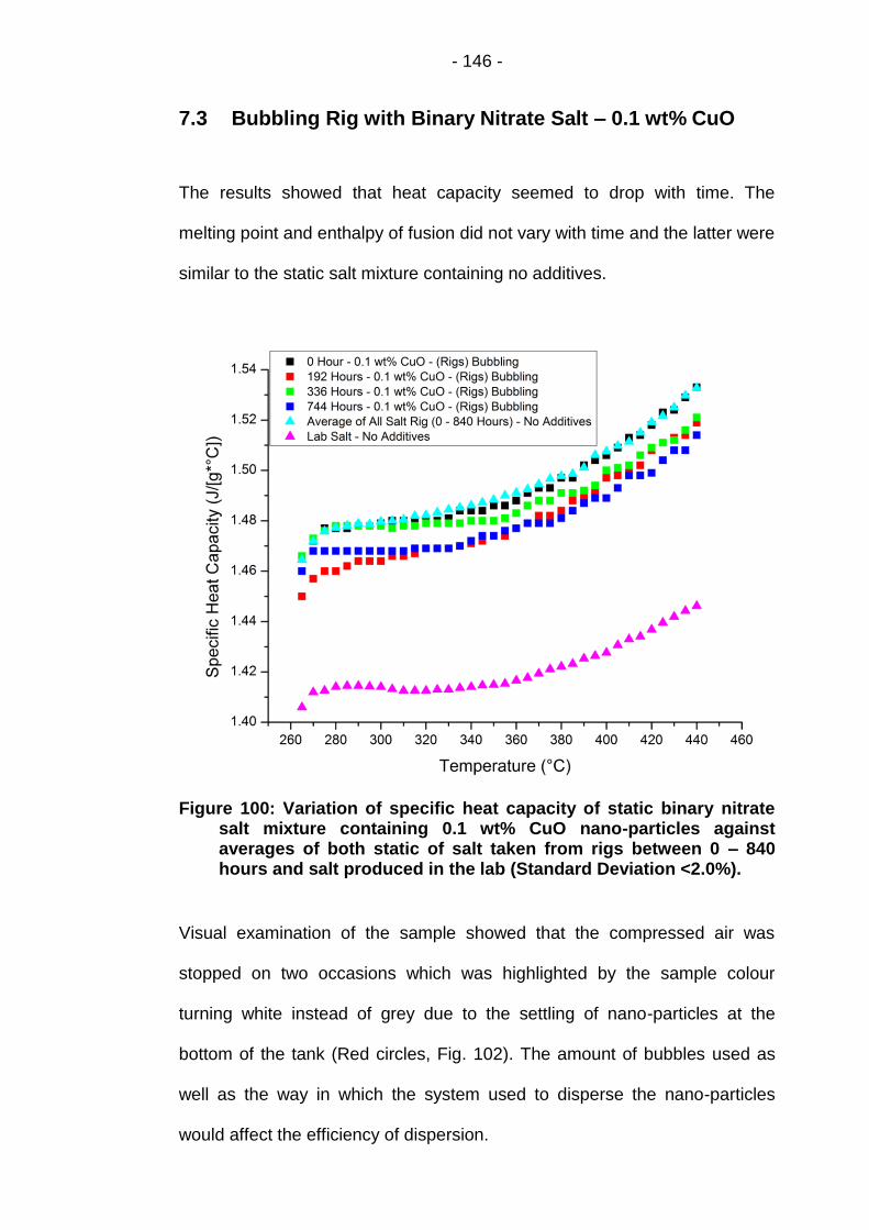
- 146 -

7.3 Bubbling Rig with Binary Nitrate Salt – 0.1 wt% CuO

The results showed that heat capacity seemed to drop with time. The

melting point and enthalpy of fusion did not vary with time and the latter were

similar to the static salt mixture containing no additives.


Visual examination of the sample showed that the compressed air was

stopped on two occasions which was highlighted by the sample colour

turning white instead of grey due to the settling of nano-particles at the

bottom of the tank (Red circles, Fig. 102). The amount of bubbles used as

well as the way in which the system used to disperse the nano-particles

would affect the efficiency of dispersion.

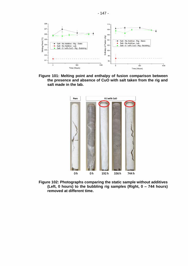
- 147 -


Figure 102: Photographs comparing the static sample without additives (Left, 0 hours) to the bubbling rig samples (Right, 0 – 744 hours) removed at different time.

- 148 -

7.4 Dynamic Rig with Binary Nitrate Salt – 0.1 wt% CuO

This type of dispersion had a negative impact on the specific heat capacity,

which was far more pronounced than bubbling. The latter increased with

time, coming close to the value obtained for specific heat capacity of pure

salt produced in the lab.


Only two samples were collected due to a failure of the piston preventing the

collection of further samples. No real differences were measured in both the

enthalpy of fusion and the melting point.

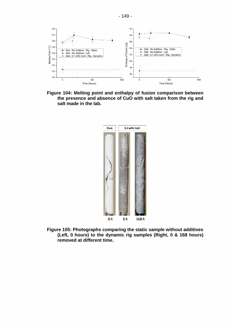
- 149 -


Figure 105: Photographs comparing the static sample without additives (Left, 0 hours) to the dynamic rig samples (Right, 0 & 168 hours) removed at different time.

- 150 -

7.5 Stirring Rig (400 rpm) with Binary Nitrate Salt – 0.1 wt%

CuO

The mean specific heat capacity displayed a rise after 576 & 744 Hours

when stirring at 400 rpm whilst below 240 hours; the specific heat capacity

was similar to that of the average value of rig salt containing no additive.


No differences were showed in the melting point; however the enthalpy of

fusion was significantly lowered consistently through the duration of the

tests. Finally visual analysis showed that the use of stirring kept the

colouration of the salt similar which could be an indication of dispersion.

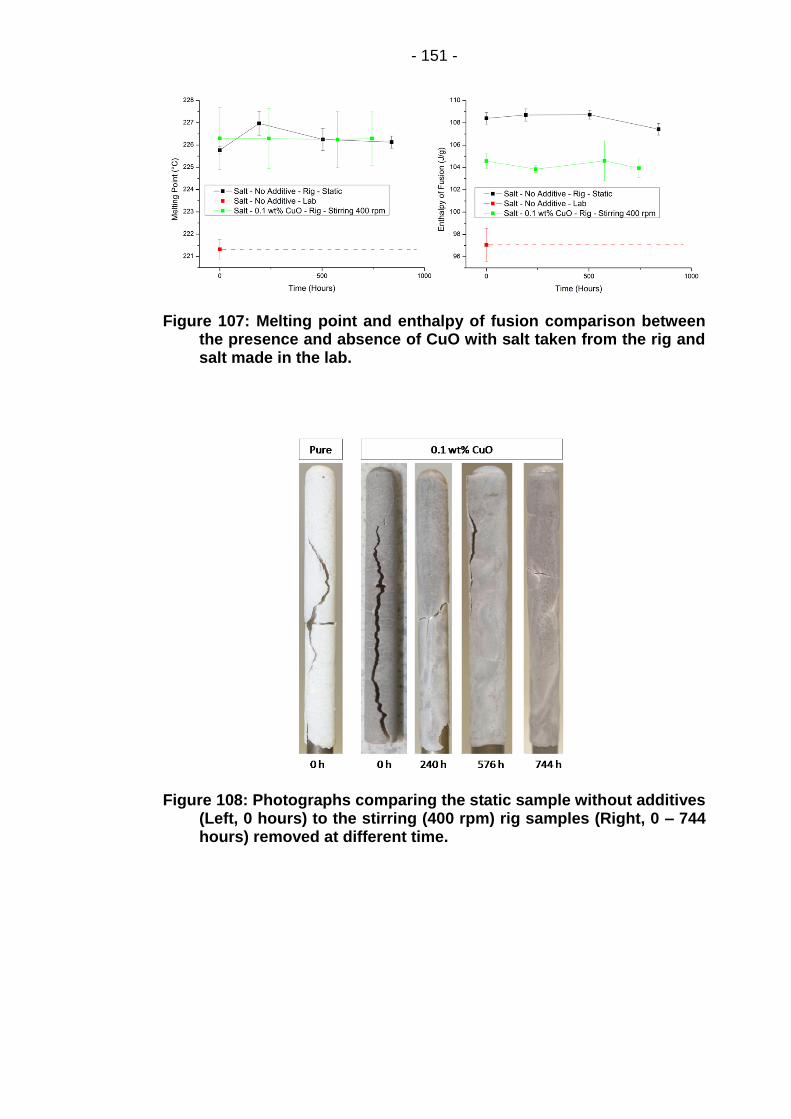
- 151 -


Figure 108: Photographs comparing the static sample without additives (Left, 0 hours) to the stirring (400 rpm) rig samples (Right, 0 – 744 hours) removed at different time.

- 152 -

7.6 Further Discussion and Summary

The addition of nano-particles to binary mixture of nitrate salt revealed that

settling was a challenge to overcome in order to profit from their beneficial

effect particularly on the specific heat capacity. Providing that this

enhancement was due to the production of these nano-layers, variables

such as size distribution of the nano-particles, percentage ratio of additives,

surface chemistry of nano-particle & shape, type of container used, salt ratio

& type, temperature, viscosity and probably many others factors will affect

their behaviour. As it was demonstrated previously, the optimum ratio is

different from one type of nano-particle to the next. The use of physical

dispersion provided a mean to re-suspend the copper oxide nano-particles.

However the type of dispersion used altered the specific heat capacity

measurement such that both bubbling and dynamic impacted negatively on

the mixture whilst only stirring provided an increase in the mean Cp values

which differed greatly from results observed in the lab. The type of

turbulence used might have reduced/disturbed the production of these nano-

layers around the copper oxide nano-particles leading to a decrease in Cp.

Alternatively the method of dispersion which was different as large scale

production was needed, might have altered the surface chemistry of the

nano-particle significantly such that the results obtained were altered.

The general trend in the melting point and enthalpy of fusion seemed to be a

slight decrease in the value tested compared to the static pure salt value.

The only exception was for the stirring enthalpy of fusion which was altered

significantly whilst the melting point was similar although the standard

deviation was greater.

- 153 -

Chapter 8 Conclusion and Future Work

The aim of this thesis was to try to understand how the thermal behaviour of

binary nitrate mixture of salt was altered by the addition of nano-particles.

The specific objectives were as followed:

I. Define the thermal characteristics of potassium and sodium nitrate as

well as the eutectic nitrate mixture of the latter two (60 wt% NaNO3 +

40 wt% KNO3)

II. Screen how the addition of nano-particles affect the specific heat

capacity of the salt mixture

III. Evaluate whether the methodology of dispersion affect the value

obtained for specific heat capacity and how melting, onset and

crystallisation react to such change

IV. Characterise the rheology of the selected additive

V. Analyse the behaviour of the selected nano-particle (0.1 wt% CuO) on

salt before and after melting has occurred using SEM

VI. Test whether physical dispersion affects the thermal properties of the

salt over time.

(I) Sodium and potassium nitrate displayed melting point of 308.01°C and

336.03°C respectively with enthalpy of fusion of 172.84 J/g for NaNO3 and

95.55 J/g for KNO3. The specific heat capacity was found to be 1.30 J/[g*°C]

for KNO3 at 350°C whilst NaNO3 was 1.50 J/[g*°C]. The combination of

these two salts (60 wt% NaNO3 & 40 wt% KNO3) led to the production of a

- 154 -

eutectic mixture which had a melting point of 221°C as expected with

enthalpy of fusion of 97.06 J/g. The calculation of Cp closely matched the

actual measured values with values of 1.415 J/[g*°C] against the 1.42

J/[g*°C] calculated. This eutectic salt was showed to be stable up to 550°C

and rheological measurement revealed a Newtonian behaviour above shear

rate of 100 s-1. The viscosity dropped with increasing temperature from 4.75

mPa.s at 250°C to 1.75 mPa.s at 450°C which seemed to follow the

literature value obtained.

(II) The addition of nano-particles to molten salt had an overall positive effect

on the specific heat capacity raising the mean value of the salt.

Consequently the onset melting temperature dropped and the range of the

melting increased as well as the enthalpy of fusion. The onset and peak of

crystallisation were also both affect by the nano-particle addition causing an

increase in both values.

(III) The evaluation of the methodology revealed no difference in the heat

capacity values between the techniques used to prepare the samples. This

was important to know as this technique could be scaled up to industrial

level.

(IV) The rheology of the salt with nano-particle additive showed a slight

increase in viscosity as the nano-particles disturbed the flow lines.

(V) SEM images of 0.1 wt% CuO revealed that the interaction between the

salt surface before and after melting were present. It also showed

- 155 -

heterogeneous distribution of nano-particles which could have a major

impact on the specific heat capacity of salt due to a reduction of the nano-

layers total volume through aggregation. Furthermore it revealed the

importance attached to nano-particles production, as the surface chemistry

as well as shape of the nano-particles is going to be affected by the

production process. This will also impact dispersion.

(VI) The behaviour of salt in the rigs was different from the tests carried out

in the DSC. The melting, crystallisation and enthalpy of change varied

between the two when only pure salt was used. A number of reasons were

enumerated for this change, but the exact cause of the change was not

defined.

The tests also revealed the settling challenge encountered when using

nano-particles and showed that the type of physical dispersion used to re-

suspend the nano-particles could affect the specific heat capacity either

negatively or positively. The enhancement seen during the screening test

(10% increase using 0.1 wt% CuO) was not repeated in the rig tests.

The research carried out led to more question been raised than answered

and highlighted how the need for further research in the following area:

Effect of nano-particles production process and salt mixing method

on the specific heat capacity of salt

Investigation on the stability of nano-particles with varying

temperature

Testing how physical dispersion of different concentration of nano-

particles affects the specific heat capacity

- 156 -

Modelling of ionic interaction of molten salt ions with nano-particles

Industrial application of salt in concentrated solar power plant is still hindered

by the lack of knowledge and fundamental understanding of the behaviour of

nano-particles in liquid molten salt. Tackling each of the above issues might

provide a way toward the application of this technology which would reduce

the cost of electricity production allowing it to compete with non-renewable

technology in the production of electricity.

- 157 -

List of References

1. Manzano-Agugliaro, F., et al., Scientific production of renewable energies worldwide: An overview. Renewable & Sustainable Energy Reviews, 2013. 18: p. 134-143.

2. Kadiri, M., et al., A review of the potential water quality impacts of tidal renewable energy systems. Renewable & Sustainable Energy Reviews, 2012. 16(1): p. 329-341.

3. IEA, International Energy Outlook 2011. 2011, International Energy Agency: http://www.eia.gov/forecasts/ieo/pdf/0484(2011).pdf.

4. IEA. Key World Energy STATISTICS. 2012; Available from: http://www.iea.org/publications/freepublications/publication/kwes.pdf.

5. Dincer, I. and M.A. Rosen, Energy, environment and sustainable development. Applied Energy, 1999. 64(1-4): p. 427-440.

6. Thirugnanasambandam, M., S. Iniyan, and R. Goic, A review of solar thermal technologies. Renewable & Sustainable Energy Reviews, 2010. 14(1): p. 312-322.

7. Kalogirou, S.A., Solar thermal collectors and applications. Progress in Energy and Combustion Science, 2004. 30(3): p. 231-295.

8. IRENA, Concentrating Solar Power. 2012, International Renewable Energy Agency (IRENA).

9. IRENA, Concentrated Solar Power. 2013, International Renewable Energy Agency (IRENA).

10. Dell, R.M. and D.A.J. Rand, Energy storage - a key technology for global energy sustainability. Journal of Power Sources, 2001. 100(1-2): p. 2-17.

11. IEA, Solar Energy Perspectives. 2011, International Energy Agency. 12. Kenisarin, M.M., High-temperature phase change materials for

thermal energy storage. Renewable & Sustainable Energy Reviews, 2010. 14(3): p. 955-970.

13. Shin, D. and D. Banerjee, Effects of silica nanoparticles on enhancing the specific heat capacity of carbonate salt eutectic (work in progress). INTERNATIONAL JOURNAL OF STRUCTURAL CHANGES IN SOLIDS, 2010. 2(2): p. 25-31.

14. Tiznobaik, H. and D. Shin, Enhanced specific heat capacity of high-temperature molten salt-based nanofluids. International Journal of Heat and Mass Transfer, 2013. 57(2): p. 542-548.

15. Dudda, B. and D. Shin, Effect of nanoparticle dispersion on specific heat capacity of a binary nitrate salt eutectic for concentrated solar power applications. International Journal of Thermal Sciences, 2013. 69(0): p. 37-42.

16. Lu, M.C. and C.H. Huang, Specific heat capacity of molten salt-based alumina nanofluid. Nanoscale Research Letters, 2013. 8.

17. DOE, U.S., SunShot Vision Study : February 2012. 2012, U.S. DEPARTMENT OF ENERGY.

http://www.eia.gov/forecasts/ieo/pdf/0484(2011).pdf

http://www.iea.org/publications/freepublications/publication/kwes.pdf

- 158 -

18. NEEDS, Final report on technical data, costs, and life cycle inventories of solar thermal power plants, in NEEDS. 2008, New Energy Externalities Developments for Sustainability (NEEDS).

19. Price, H., et al., Advances in parabolic trough solar power technology. Journal of Solar Energy Engineering-Transactions of the Asme, 2002. 124(2): p. 109-125.

20. Yaghoubi, M., F. Ahmadi, and M. Bandehee, Analysis of Heat Losses of Absorber Tubes of Parabolic through Collector of Shiraz (Iran) Solar Power Plant. Journal of Clean Energy Technologies, 2013. 1(1): p. 5.

21. Mills, D.R. and G.L. Morrison, Compact linear Fresnel reflector solar thermal powerplants. Solar Energy, 2000. 68(3): p. 263-283.

22. Mills, D.R., G.L. Morrison, and P. Le Liever. MULTI-TOWER LINE FOCUS FRESNEL ARRAYS. in International Solar Energy Conference. 2003. Mauna Kea Resort, Hawaii Island, Hawaii, USA: ASME.

23. Mills, D., Advances in solar thermal electricity technology. Solar Energy, 2004. 76(1-3): p. 19-31.

24. Lovegrove, K., et al., Concentrating Solar Power in India [Report commissioned by the Australian Government and prepared by IT Power]. 2011, Australian Government: Department of Climate Change and energy Efficiency

25. Mancini, T., et al., Dish-Stirling systems: An overview of development and status. Journal of Solar Energy Engineering-Transactions of the Asme, 2003. 125(2): p. 135-151.

26. Kongtragool, B. and S. Wongwises, A review of solar-powered Stirling engines and low temperature differential Stirling engines. Renewable & Sustainable Energy Reviews, 2003. 7(2): p. 131-154.

27. IEA, Technology Roadmap: Concentrating Solar Power. 2010, International Energy Agency.

28. Zhang, H.L., et al., Concentrated solar power plants: Review and design methodology. Renewable & Sustainable Energy Reviews, 2013. 22: p. 466-481.

29. Pavlovic, T.M., et al., A review of concentrating solar power plants in the world and their potential use in Serbia. Renewable & Sustainable Energy Reviews, 2012. 16(6): p. 3891-3902.

30. Schramek, P. and D.R. Mills, Multi-tower solar array. Solar Energy, 2003. 75(3): p. 249-260.

31. Py, X., Y. Azoumah, and R. Olives, Concentrated solar power: Current technologies, major innovative issues and applicability to West African countries. Renewable & Sustainable Energy Reviews, 2013. 18: p. 306-315.

32. Sengupta, M., et al., INTRODUCING NREL’S BEST PRACTICES HANDBOOK FOR COLLECTION AND USE OF SOLAR RESOURCE DATA FOR CSP, in IV Conferencia Latino Americana de Energía Solar. 2010: Cusco, Peru.

33. Powell, K.M. and T.F. Edgar, Modeling and control of a solar thermal power plant with thermal energy storage. Chemical Engineering Science, 2012. 71: p. 138-145.

- 159 -

34. Medrano, M., et al., State of the art on high-temperature thermal energy storage for power generation. Part 2-Case studies. Renewable & Sustainable Energy Reviews, 2010. 14(1): p. 56-72.

35. Steinmann, W.D. and M. Eck, Buffer storage for direct steam generation. Solar Energy, 2006. 80(10): p. 1277-1282.

36. Pacheco, J.E., S.K. Showalter, and W.J. Kolb, Development of a molten-salt thermocline thermal storage system for parabolic trough plants. Journal of Solar Energy Engineering-Transactions of the Asme, 2002. 124(2): p. 153-159.

37. Fang, M. and G.M. Chen, Effects of different multiple PCMs on the performance of a latent thermal energy storage system. Applied Thermal Engineering, 2007. 27(5-6): p. 994-1000.

38. Bauer, T., D. Laing, and R. Tamme, Overview of PCMs for concentrated solar power in the temperature range 200 to 350 °C. Advances in Science and Technology, 2010. 74: p. 272-277.

39. Laing, D., et al., Solid media thermal storage for parabolic trough power plants. Solar Energy, 2006. 80(10): p. 1283-1289.

40. Laing, D., et al., High-Temperature Solid-Media Thermal Energy Storage for Solar Thermal Power Plants. Proceedings of the Ieee, 2012. 100(2): p. 516-524.

41. Laing, D., et al., Test Results of Concrete Thermal Energy Storage for Parabolic Trough Power Plants. Journal of Solar Energy Engineering-Transactions of the Asme, 2009. 131(4).

42. Kuravi, S., et al., Thermal energy storage technologies and systems for concentrating solar power plants. Progress in Energy and Combustion Science, 2013. 39(4): p. 285-319.

43. Levy, M., et al., SOLAR-ENERGY STORAGE VIA A CLOSED-LOOP CHEMICAL HEAT PIPE. Solar Energy, 1993. 50(2): p. 179-189.

44. Lovegrove, K., et al., Developing ammonia based thermochemical energy storage for dish power plants. Solar Energy, 2004. 76(1-3): p. 331-337.

45. Kanamori, M., H. Matsuda, and M. Hasatani, Heat storing/releasing characteristics of the chemical heat storing unit of electricity using Ca(OH)(2)/CaO reaction. Kagaku Kogaku Ronbunshu, 1996. 22(2): p. 257-263.

46. Schaube, F., A. Worner, and R. Tamme, High Temperature Thermochemical Heat Storage for Concentrated Solar Power Using Gas-Solid Reactions. Journal of Solar Energy Engineering-Transactions of the Asme, 2011. 133(3).

47. Abhat, A., LOW-TEMPERATURE LATENT-HEAT THERMAL-ENERGY STORAGE - HEAT-STORAGE MATERIALS. Solar Energy, 1983. 30(4): p. 313-332.

48. Farid, M.M., et al., A review on phase change energy storage: materials and applications. Energy Conversion and Management, 2004. 45(9-10): p. 1597-1615.

49. Shiina, Y. and T. Inagaki, Study on the efficiency of effective thermal conductivities on melting characteristics of latent heat storage capsules. International Journal of Heat and Mass Transfer, 2005. 48(2): p. 373-383.

- 160 -

50. Nomura, T., N. Okinaka, and T. Akiyama, Technology of Latent Heat Storage for High Temperature Application: A Review. Isij International, 2010. 50(9): p. 1229-1239.

51. Zhang, X.X., et al., Expansion space and thermal stability of microencapsulated n-octadecane. Journal of Applied Polymer Science, 2005. 97(1): p. 390-396.

52. Fang, Y.T., et al., Preparation and characterization of novel nanoencapsulated phase change materials. Energy Conversion and Management, 2008. 49(12): p. 3704-3707.

53. Fang, Y.T., et al., Preparation of nanoencapsulated phase change material as latent functionally thermal fluid. Journal of Physics D-Applied Physics, 2009. 42(3).

54. Tamme, R., et al., Latent heat storage above 120 degrees C for applications in the industrial process heat sector and solar power generation. International Journal of Energy Research, 2008. 32(3): p. 264-271.

55. Wu, J.F., et al., Molten salts/ceramic-foam matrix composites by melt infiltration method as energy storage material. Journal of Wuhan University of Technology-Materials Science Edition, 2009. 24(4): p. 651-653.

56. Kodama, T., et al., Ni/ceramic/molten-salt composite catalyst with high-temperature thermal storage for use in solar reforming processes. Energy, 2004. 29(5-6): p. 895-903.

57. Kodama, T., et al., Molten-Salt Tubular Absorber/Reformer (MoSTAR) Project: The Thermal Storage Media of Na2CO3-MgO Composite Materials. Journal of Solar Energy Engineering-Transactions of the Asme, 2009. 131(4).

58. Mondieig, D., et al., Protection of temperature sensitive biomedical products using molecular alloys as phase change material. Transfusion and Apheresis Science, 2003. 28(2): p. 143-148.

59. Dincer, I. and S. Dost, A perspective on thermal energy storage systems for solar energy applications. International Journal of Energy Research, 1996. 20(6): p. 547-557.

60. Hasnain, S.M., Review on sustainable thermal energy storage technologies, part I: Heat storage materials and techniques. Energy Conversion and Management, 1998. 39(11): p. 1127-1138.

61. Dincer, I., S. Dost, and X.G. Li, Performance analyses of sensible heat storage systems for thermal applications. International Journal of Energy Research, 1997. 21(12): p. 1157-1171.

62. Choi, S.U.S. and J.A. Eastman, Enhancing Thermal Conductivity of Fluids with Nano-particles, in International Mechanical Engineering Congress & Exposition. 1995: San Francisco, USA.

63. Lee, S., et al., Measuring thermal conductivity of fluids containing oxide nanoparticles. Journal of Heat Transfer-Transactions of the Asme, 1999. 121(2): p. 280-289.

64. Das, S.K., et al., Temperature dependence of thermal conductivity enhancement for nanofluids. Journal of Heat Transfer-Transactions of the Asme, 2003. 125(4): p. 567-574.

65. Patel, H.E., et al., Thermal conductivities of naked and monolayer protected metal nanoparticle based nanofluids: Manifestation of

- 161 -

anomalous enhancement and chemical effects. Applied Physics Letters, 2003. 83(14): p. 2931-2933.

66. Wen, D.S. and Y.L. Ding, Experimental investigation into convective heat transfer of nanofluids at the entrance region under laminar flow conditions. International Journal of Heat and Mass Transfer, 2004. 47(24): p. 5181-5188.

67. Wen, D.S. and Y.L. Ding, Formulation of nanofluids for natural convective heat transfer applications. International Journal of Heat and Fluid Flow, 2005. 26(6): p. 855-864.

68. Xie, H.Q., et al., Dependence of the thermal conductivity of nanoparticle-fluid mixture on the base fluid. Journal of Materials Science Letters, 2002. 21(19): p. 1469-1471.

69. Zhang, X., H. Gu, and M. Fujii, Effective thermal conductivity and thermal diffusivity of nanofluids containing spherical and cylindrical nanoparticles. Experimental Thermal and Fluid Science, 2007. 31(6): p. 593-599.

70. Eastman, J.A., et al., Anomalously increased effective thermal conductivities of ethylene glycol-based nanofluids containing copper nanoparticles. Applied Physics Letters, 2001. 78(6): p. 718-720.

71. He, Y.R., et al., Heat transfer and flow behaviour of aqueous suspensions of TiO2 nanoparticles (nanofluids) flowing upward through a vertical pipe. International Journal of Heat and Mass Transfer, 2007. 50(11-12): p. 2272-2281.

72. Ding, Y.L., et al., Heat transfer of aqueous suspensions of carbon nanotubes (CNT nanofluids). International Journal of Heat and Mass Transfer, 2006. 49(1-2): p. 240-250.

73. Ding, Y.L., et al., Heat Transfer Intensification Using Nanofluids. Kona-Powder and Particle, 2007. 25: p. 23-38.

74. Xie, H.Q., et al., Thermal conductivity enhancement of suspensions containing nanosized alumina particles. Journal of Applied Physics, 2002. 91(7): p. 4568-4572.

75. Keblinski, P., R. Prasher, and J. Eapen, Thermal conductance of nanofluids: is the controversy over? Journal of Nanoparticle Research, 2008. 10(7): p. 1089-1097.

76. Buongiorno, J., et al., A benchmark study on the thermal conductivity of nanofluids. Journal of Applied Physics, 2009. 106(9).

77. Trisaksri, V. and S. Wongwises, Critical review of heat transfer characteristics of nanofluids. Renewable & Sustainable Energy Reviews, 2007. 11(3): p. 512-523.

78. Yu, W. and H. Xie, A Review on Nanofluids: Preparation, Stability Mechanisms, and Applications. Journal of Nanomaterials, 2012.

79. Yang, X. and Z.-h. Liu, A Kind of Nanofluid Consisting of Surface-Functionalized Nanoparticles. Nanoscale Research Letters, 2010. 5(8): p. 1324-1328.

80. Prasher, R., P.E. Phelan, and P. Bhattacharya, Effect of aggregation kinetics on the thermal conductivity of nanoscale colloidal solutions (nanofluid). Nano Letters, 2006. 6(7): p. 1529-1534.

81. Lee, D., J.W. Kim, and B.G. Kim, A new parameter to control heat transport in nanofluids: Surface charge state of the particle in suspension. Journal of Physical Chemistry B, 2006. 110(9): p. 4323-4328.

- 162 -

82. Das, S.K., S.U.S. Choi, and H.E. Patel, Heat transfer in Nanofluids - A review. Heat Transfer Engineering, 2006. 27(10): p. 3-19.

83. Xuan, Y.M. and Q. Li, Heat transfer enhancement of nanofluids. International Journal of Heat and Fluid Flow, 2000. 21(1): p. 58-64.

84. Bolmatov, D., V.V. Brazhkin, and K. Trachenko, The phonon theory of liquid thermodynamics. Sci. Rep., 2012. 2.

85. Zhou, S.-Q. and R. Ni, Measurement of the specific heat capacity of water-based Al(2)O(3) nanofluid. Applied Physics Letters, 2008. 92(9).

86. Pantzali, M.N., et al., Effect of nanofluids on the performance of a miniature plate heat exchanger with modulated surface. International Journal of Heat and Fluid Flow, 2009. 30(4): p. 691-699.

87. Pak, B.C. and Y.I. Cho, Hydrodynamic and heat transfer study of dispersed fluids with submicron metallic oxide particles. Experimental Heat Transfer, 1998. 11(2): p. 151-170.

88. Saeedinia, M., M.A. Akhavan-Behabadi, and P. Razi, Thermal and rheological characteristics of CuO-Base oil nanofluid flow inside a circular tube. International Communications in Heat and Mass Transfer, 2012. 39(1): p. 152-159.

89. Nelson, C., I., CHARACTERIZATION OF THERMO-PHYSICAL PROPERTIES AND FORCED CONVECTIVE HEAT TRANSFER OF POLY-ALPHA-OLEFIN (PAO) NANOFLUIDS. 2007, Texas A&M University: Texas, USA. p. 81.

90. Shin, D.H. and D. Banerjee, Enhanced Specific Heat of Silica Nanofluid. Journal of Heat Transfer-Transactions of the Asme, 2011. 133(2).

91. Wang, L., et al., Enhancement of molar heat capacity of nanostructured Al2O3. Journal of Nanoparticle Research, 2001. 3(5-6): p. 483-487.

92. Tan, Z.C., L. Wang, and Q. Shi, Study of heat capacity enhancement in some nanostructured materials. Pure and Applied Chemistry, 2009. 81(10): p. 1871-1880.

93. Tiznobaik, H. and D. Shin, Experimental validation of enhanced heat capacity of ionic liquid-based nanomaterial. Applied Physics Letters, 2013. 102(17).

94. Shin, D. and D. Banerjee, Enhancement of specific heat capacity of high-temperature silica-nanofluids synthesized in alkali chloride salt eutectics for solar thermal-energy storage applications. International Journal of Heat and Mass Transfer, 2011. 54(5-6): p. 1064-1070.

95. Wang, B.X., L.P. Zhou, and X.F. Peng, Surface and size effects on the specific heat capacity of nanoparticles. International Journal of Thermophysics, 2006. 27(1): p. 139-151.

96. Prasher, R., P. Bhattacharya, and P.E. Phelan, Brownian-motion-based convective-conductive model for the effective thermal conductivity of nanofluids. Journal of Heat Transfer-Transactions of the Asme, 2006. 128(6): p. 588-595.

97. Xue, L., et al., Effect of liquid layering at the liquid–solid interface on thermal transport. International Journal of Heat and Mass Transfer, 2004. 47(19–20): p. 4277-4284.

98. Oh, S.H., et al., Ordered liquid aluminum at the interface with sapphire. Science, 2005. 310(5748): p. 661-663.

- 163 -

99. Rheotec. Introduction to Rheology: Basics. Available from: http://www.dongjins.com/service/file/Introduction%20to%20rheology.pdf.

100. Schramm, G. A Practical Approach to Rheology and Rheometry. 1994; Available from: http://www.asi-team.com/asi%20team/haake/haake%20data/A%20practical%20approach%20to%20rheology%20and%20rhometry.pdf.

101. Kestin, J., M. Sokolov, and W.A. Wakeham, VISCOSITY OF LIQUID WATER IN RANGE -8-DEGREES-C TO 150-DEGREES-C. Journal of Physical and Chemical Reference Data, 1978. 7(3): p. 941-948.

102. Rheotek. VISCOSITY OIL STANDARDS. 2014; Available from: http://www.rheotek.com/assets/rheotek/sub_cat_docs/Viscosity%20Oil%20Standards.pdf.

103. Janz, G., Molten Salts Data as Reference Standards for Density, Surface Tension, Viscosity and Electrical Conductance: KNO3 and NaCl. Journal of Physical and Chemical Reference Data, 1980. 9(4): p. 39.

104. Laing, D., et al., Advanced High Temperature Latent Heat Storage system - Design and Test Results, in Effstock 2009. 2009: Stockholm, Sweden.

105. Bauer, T., et al., SODIUM NITRATE FOR HIGH TEMPERATURE LATENT HEAT STORAGE, in Effstock 2009. 2009: Stockholm, Sweden.

106. Takahashi, Y., R. Sakamoto, and M. Kamimoto, HEAT-CAPACITIES AND LATENT HEATS OF LINO3, NANO3, AND KNO3. International Journal of Thermophysics, 1988. 9(6): p. 1081-1090.

107. Carling, R.W., HEAT-CAPACITIES OF NANO3 AND KNO3 FROM 350-K TO 800-K. Thermochimica Acta, 1983. 60(3): p. 265-275.

108. Bauer, T., et al., Material aspects of Solar Salt for sensible heat storage. Applied Energy, 2013. 111: p. 1114-1119.

109. Instrument, T. Sapphire Specific Heat Capacity Literature Values. 2014; Available from: http://www.tainstruments.co.jp/application/pdf/Thermal_Library/Applications_Notes/TN008.PDF.

110. Bauer, T. PCM-Graphite Composites for High Temperature Thermal Energy Storage. 2006; Available from: http://intraweb.stockton.edu/eyos/energy_studies/content/docs/FINAL_PRESENTATIONS/8B-1.pdf.

111. Betts, M., THE EFFECTS OF NANOPARTICLE AUGMENTATION OF NITRATE THERMAL STORAGE MATERIALS FOR USE IN CONCENTRATING SOLAR POWER APPLICATIONS, in Mechanical Engineering. 2011, Texas A&M University: Texas, USA. p. 91.

112. Steinmann, W.D., D. Laing, and R. Tamme, Development of PCM Storage for Process Heat and Power Generation. Journal of Solar Energy Engineering-Transactions of the Asme, 2009. 131(4).

113. Kearney, D., et al., Assessment of a molten salt heat transfer fluid in a parabolic trough solar field. Journal of Solar Energy Engineering-Transactions of the Asme, 2003. 125(2): p. 170-176.

114. Stern, H.K., High Temperature Properties and Decomposition of Inorganic Salts

http://www.dongjins.com/service/file/Introduction%20to%20rheology.pdf

http://www.dongjins.com/service/file/Introduction%20to%20rheology.pdf

http://www.asi-team.com/asi%20team/haake/haake%20data/A%20practical%20approach%20to%20rheology%20and%20rhometry.pdf



http://www.rheotek.com/assets/rheotek/sub_cat_docs/Viscosity%20Oil%20Standards.pdf

http://www.rheotek.com/assets/rheotek/sub_cat_docs/Viscosity%20Oil%20Standards.pdf

http://www.tainstruments.co.jp/application/pdf/Thermal_Library/Applications_Notes/TN008.PDF

http://www.tainstruments.co.jp/application/pdf/Thermal_Library/Applications_Notes/TN008.PDF

http://intraweb.stockton.edu/eyos/energy_studies/content/docs/FINAL_PRESENTATIONS/8B-1.pdf

http://intraweb.stockton.edu/eyos/energy_studies/content/docs/FINAL_PRESENTATIONS/8B-1.pdf

- 164 -

Part3. Nitrates and Nitrites. Journal of Physical and Chemical Reference Data, 1972. 1(3): p. 25.

115. Kramer, C.M. and C.J. Wilson, The phase diagram of NaNO3—KNO3. Thermochimica Acta, 1980. 42(3): p. 253-264.

116. Siegel, N.P., et al., THERMOPHYSICAL PROPERTY MEASUREMENT OF NITRATE SALT HEAT TRANSFER FLUIDS. Proceedings of the Asme 5th International Conference on Energy Sustainability 2011, Pts a-C. 2012. 439-446.

117. Nissen, A.D., Thermophysical Properties of the Equimolar Mixture NaNO3-KNO3 from 300 to 600°C. Journal of Chemical and Engineering Data, 1982. 27(3): p. 4.

118. Janz, J.G., et al., Physical Properties Data Compilations Relevant to Energy Storage – II. Molten salts: Data on single and multi-component salt. 1979, National Bureau of Standards.

119. Chieruzzi, M., et al., Effect of nanoparticles on heat capacity of nanofluids based on molten salts as PCM for thermal energy storage. Nanoscale Research Letters, 2013(8): p. 448.

120. Nash, L.K., Elements of Statistical Thermodynamics, 2nd Edition. 1972, USA: Dover Publications.

121. Singh, N., COMPUTATIONAL ANALYSIS OF THERMO-FLUIDIC CHARACTERISTICS OF A CARBON NANO-FIN, in Mechanical Engineering. 2010, Texas: Texas, USA. p. 114.

122. Keblinski, P., J.A. Eastman, and D.G. Cahill, Nanofluids for thermal transport. Materials Today, 2005. 8(6): p. 36-44.

123. Ren, Y., H. Xie, and A. Cai, Effective thermal conductivity of nanofluids containing spherical nanoparticles. Journal of Physics D-Applied Physics, 2005. 38(21): p. 3958-3961.

124. Jo, B. and D. Banerjee, Enhanced specific heat capacity of molten salt-based nanomaterials: Effects of nanoparticle dispersion and solvent material. Acta Materialia, 2014. 75: p. 80-91.

125. Jo, B., et al., ANOMALOUS RHEOLOGICAL BEHAVIOR OF COMPLEX FLUIDS (NANOFLUIDS). Proceedings of the Asme International Mechanical Engineering Congress and Exposition, 2011, Vol 6, Pts a and B. 2012, New York: Amer Soc Mechanical Engineers. 223-228.

126. Chen, H., Y. Ding, and C. Tan, Rheological behaviour of nanofluids. New Journal of Physics, 2007. 9.

127. Rao, Y., Nanofluids: Stability, phase diagram, rheology and applications. Particuology, 2010. 8(6): p. 549-555.

128. Mishra, P.C., et al., A brief review on viscosity of nanofluids. International Nano Letters, 2014.

129. Rudyak, V., Viscosity of Nanofluids—Why It Is Not Described by the Classical Theories. Advances in Nanoparticles, 2013. 2: p. 266-279.

130. Litchfield, D.W. and G. Baird, THE RHEOLOGY OF HIGH ASPECT RATIO NANOPARTICLE FILLED LIQUIDS. The British Society of Rheology, 2006: p. 1-60.

131. Andreu-Cabedo, P., et al., Increment of specific heat capacity of solar salt with SiO2 nanoparticles. Nanoscale research letters, 2014. 9(1): p. 582-582.

- 165 -

132. Bradshaw, R.W. and H. Goods, S., Effect of Temperature on Corrosion of Type 316 SS by Molten NaNO3 – KNO3, in ElectroChemistry Society (ECS). 2000: Toronto, Canada.

nitrate based high temperature nano-heat-transfer-fluids...

Documents