heat transfer & periodic flow analysis of heat exchanger by cfd with nano fluids

Ms. N.Gayathri et al. Int. Journal of Engineering Research and Applications www.ijera.com

ISSN: 2248-9622, Vol. 6, Issue 1, (Part - 1) January 2016, pp.43-66

www.ijera.com 43|P a g e

Heat Transfer & Periodic Flow Analysis of Heat Exchanger by

CFD with Nano Fluids

Ms. N.Gayathri1, Mr.V.V.Ramakrishna M.Tech

2, Mr. Sanmala Rajasekhar

3

M.Tech(P.Hd) 1 M.Tech Student Department Of Mechanical Engg, KITS Engineering College, Divilia.P, India, 533433.

2Asst Professor Department Of Mechanical Engg, KITS Engineering College, Divili, A.P, India, 533433.

3Assoc.Professor Department Of Mechanical Engg, KITS Engineering College, Divilia.P, India, 533433.

Abstract Many heat transfer applications such as steam generators in a boiler or air cooling coil of an air conditioner, can

be modelled in a bank of tubes containing a fluid flowing at one temperature that is immersed in a second fluid

in a cross flow at different temperature. CFD simulations are a useful tool for understanding flow and heat

transfer principles as well as for modelling these types of geometries. Both the fluids considered in the present

study are CUO Nano fluids, and flow is classified as laminar and steady with Reynolds number between 100-

600.The mass flow rate of the cross flow and diameter has been varied (such as 0.05, 0.1, 0.15, 0.20, 0.25, 0.30

kg/sec and 0.8, 1.0.1.2 &1.4cm) and the models are used to predict the flow and temperature fields that result

from convective heat transfer. Due to symmetry of the tube bank and the periodicity of the flow inherent in the

tube bank geometry, only a portion of the geometry will be modelled and with symmetry applied to the outer

boundaries. The inflow boundary will be redefined as a periodic zone and the outflow boundary is defined as the

shadow. The various static pressures, velocities, and temperatures obtained are reported.

In this present project tubes of different diameters and different mass flow rates are considered to examine the

optimal flow distribution. Further the problem has been subjected to effect of materials used for tubes

manufacturing on heat transfer rate. Materials considered are copper and Nickle Chromium alloys. Results

emphasize the utilization of alloys in place of copper as tube material serves better heat transfer with most

economical way.

Keywords: Heat transfer, Heat exchanger, Nano fluids, Mass flow rate, Periodic flow, Nusselt number &

Reynolds number.

I. Introduction Generally in any kind of heat exchanger the

commonly used flowing fluid is water. But now here

we are using Nano fluid (CUO). A Nano fluid is a

fluid containing nanometre-sized particles, called

nanoparticles. These fluids are engineered colloidal

suspensions of nanoparticles in a base fluid. The

nanoparticles used in Nano fluids are typically made

of metals, oxides, carbides, or carbon nanotubes.

Common base fluids include water, ethylene

glycol and oil.

Nano fluids have novel properties that make

them potentially useful in many applications in heat

transfer including microelectronics, fuel cells ,

pharmaceutical processes, and hybrid –powered

engines, engine cooling/vehicle thermal management,

domestic refrigerator, chiller, heat exchangers in

grinding, machining and in boiler flue gas

temperature reduction. They exhibit enhanced

thermal conductivity and the convective heat

transfer coefficient compared to the base

fluid. Knowledge of the rheological behaviour of

Nano fluids is found to be very critical in deciding

their suitability for convective heat transfer

applications.In analysis such as computational fluid

dynamics (CFD), Nano fluids can be assumed to be

single phase fluids. However, almost all of new

academic paper uses two-phase assumption. Classical

theory of single phase fluids can be applied, where

physical properties of Nano fluids are taken as a

function of properties of both constituents and their

concentrations. An alternative approach simulates

Nano fluids using a two-component model. The

spreading of a Nano fluid droplet is enhanced by the

solid-like ordering structure of nanoparticles

assembled near the contact line by diffusion, which

gives rise to a structural disjoining pressurein the

vicinity of the contact line. However, such

enhancement is not observed for small droplets with

diameter of nanometre scale, because the wetting

time scale is much smaller than the diffusion time

scale.

1.1 Synthesis

Nano fluids are produced by several techniques

they are,

1. Direct Evaporation (1 step),

2. Gas condensation/dispersion (2 step),

RESEARCH ARTICLE OPEN ACCESS




3. Chemical vapour condensation (1 step),

4. Chemical precipitation (1 step).

Several liquids including water, ethylene glycol,

and oils have been used as base fluids. Nano-

materials used so far in Nano fluid synthesis

include metallic particles, oxide particles, carbon

nanotubes, graphene Nano-flakes and ceramic

particles

1.2 Applications

Nano fluids are primarily used as coolant in heat

transfer equipment such as heat exchangers,

electronic cooling system (such as flat plate) and

radiators. Heat transfer over flat plate has been

analysed by many researchers. Graphene based Nano

fluid has been found to enhance polymerase chain

reaction efficiency. Nano fluids in solar

collectors are another application where Nano fluids

are employed for their tenable optical properties.

II. Simulation& Need for CFD 2.1 Simulation

‘Simulation’ is the imitation of the operation of a

real-world process or system over time. The act of

simulating something first requires that a model to be

developed. This model represents the key

characteristics or behaviours of the selected physical

system or abstract system or process. The model

represents the system itself, whereas the simulation

represents the operation of the system over time.

Simulation is an important feature in engineering

system or any other system that involves many

processes. For example in electrical engineering,

delay lines may be used to simulate propagation

delay and phase shift caused by an

actual transmission line. Similarly, dummy loadsmay

be used to simulate impedance without simulating

propagation, and is used in situations where

propagation is unwanted. A simulator may imitate

only a few of the operations and functions of the unit

it simulates. Contrast with: emulate.

Most engineering simulations entail

mathematical modelling and computer assisted

investigation. There are many cases, however, where

mathematical modelling is not reliable. Simulations

of fluid dynamics problems often require both

mathematical and physical simulations. In these cases

the physical models require dynamic similitude.

Physical and chemical simulations have also direct

realistic uses, rather than research uses. For

example in chemical engineering, process

simulations are used to give the process parameters

immediately used for operating chemical plants such

as oil refineries.

Simulations can be categorised in different ways.

Some of them are as follows:

1. Physical simulation refers to simulation in which

physical objects are substituted for the real thing.

These physical objects are often chosen because

they are smaller or cheaper than the actual object

or system.

2. Interactive simulation is a special kind of

physical simulation, often referred to as a human

in the loopsimulation, in which physical

simulations include human operators, such as in

a flight simulator or a driving simulator. Human

in the loop simulations can include a computer

simulation as a so-called synthetic environment.

There are more different types of simulations

according to the field or stream suiting for research.

Here we are using engineering simulation with the

help of Computational Fluid Dynamics (CFD)

software.

2.2 Need for CFD

Conventional engineering analyses rely heavily

on empirical correlations so it is not possible to

obtain the results for specific flow and heat transfer

patterns in heat exchanger of arbitrary geometry.

Successful modeling of such process lies on

quantifying the heat, mass and momentum transport

phenomena. Today‟s design processes must be more

accurate while minimizing development costs to

compete in a world of economy. This forces

engineering companies to take advantage of design

tools which augment existing experience and

empirical data while minimizing cost. One tool which

excels under these conditions is CFD.

Computational Fluid Dynamics (CFD) makes it

possible to solve numerically the flow and energy

balances in complicated geometries. CFD simulates

the physical flow, heat transfer, and combustion

phenomena of solids, liquids, and gases and

executing on high speed, large memory workstations.

CFD has significant cost advantages when compared

to physical modeling and field testing and also,

provides additional insight into the physical

phenomena being analyzed due to the availability of

data that can be analyzed and the flexibility with

which geometric changes can be studied. Effective

heat transfer parameters estimated from CFD results

matched theoretical model predictions reasonably

well. Heat exchangers have been extensively

researched both experimentally and numerically.

However, most of the CFD simulation on heat

exchangers was aimed at model validation.

2.3 Simulation phenomena in heat exchangers

Hilde VAN DER VYVER, Jaco DIRKER AND

Jousa P. MEYER, who investigated the validation of

a CFD model of a three dimensional Tube-in-Tube

Heat Exchanger. The heat transfer coefficients and

the friction factors were determined with CFD and

compared to established correlations. The results

showed the reasonable agreement with empirical

correlation, while the trends were similar. When




compared with experimental data the CFD model

results showed good agreement. The average error

was 5.5% and the results compared well with

correlation. It can be concluded that the CFD

software modelled a Tube-in-Tube Heat Exchanger

in three- dimensional accurately.

2.3.1 Shell & Tube Heat Exchanger

Fig.2.3.1 Heat transfer for heat exchanger.

The second law of thermodynamics states that

heat always flows spontaneously from hotter region

to a cooler region. All active and passive devices are

sources of heat. These devices are always hotter than

the average temperature of their immediate

surroundings. There are three mechanisms for heat

transfer viz, conduction, convection and radiation.

2.3.2Heat Exchanger Tubes

Fig. 2.3.2 common tube layouts for exchangers.

The tubes are the basic components of the shell

and Tube heat exchanger, providing the heat transfer

surface between on fluid flowing inside the tube and

the other fluid flowing across outside of the tubes.

The tubes may be seamless or welded and most

commonly made of copper or steel alloys. Other

alloys for specific applications the tubes are available

in a variety of metals which includes admiralty,

Mountz metal, brass, 70-30 copper nickel, aluminium

bronze, aluminium. They are available in a number of

different wall thicknesses. Tubes in heat exchangers

are laid out on either square or triangular patterns as

shown in fig.2.3.2 The advantage of square pitch is

that the tubes are accessible for external cleaning and

cause a lower pressure drop when fluid flows in the

direction indicated in the fig.2.3.2.

2.3.3 Shell-side film coefficients

The heat transfer coefficients outside tube bundle

are referred to as shell-side coefficients. When the

tube bundle employs baffles, which serves two

functions: most importantly they support the tubes in

the proper position during assembly and operation

and prevent vibration of the tubes caused by flow-

induced eddies. Secondly they guide the shell-side

flow back and forth across the tube field, increasing

the velocity and the heat transfer coefficient.

In square pitch, as shown in fig.2.3.2 the velocity

of the fluid undergoes continuous fluctuation because

of the constricted area between adjacent tubes

compared with the flow area between successive

rows. In triangular pitch even greater turbulence is

encountered because the fluid flowing between

adjacent tubes at high velocity impinges directly on

the succeeding rows. This indicates that, when the

pressure drop and cleavability are of little

consequence, triangular pitch is superior for the

attainment of high shell-side film coefficients. This is

the actually the case, and under comparable

conditions of flow and tube size the coefficients for

triangular pitch are roughly 25% greater than for

square pitch.

2.3.4 Shell-sidemass velocity

Shell is simply the container for the shell-side

fluid. The shell is commonly has a circular cross

section and is commonly made by rolling a metal

plate of appropriate dimensions into a cylinder and




welding the longitudinal joint. In large exchangers

the shell is made out of carbon steel wherever

possible for reasons of economy. Though other alloys

can be and are used when corrosion (or) high

temperature strength demand must be met. The linear

and mass velocities of the fluid change continuously

across the bundle, since the width of the shell and

number of tube vary from row to row.

2.3.5 Shell-side Pressure Drop

The total pressure, ∆p, across a system consists

of three components:

A static pressure difference, ∆Ps ,due to the

density and elevation of the fluid.

A pressure differential, ∆P, due to the change of

momentum.

A pressure differential due to frictional losses,

∆P.

∆Pt = ∆Ps + ∆Pm + ∆Pf

2.4 Applications of Simulation

Pulverized Application

Micronized Coal Nozzle Application

Coal Gasification Application

Convection Pass Erosion Application

Scrubber Applications

Steam Drum Applicationetc,

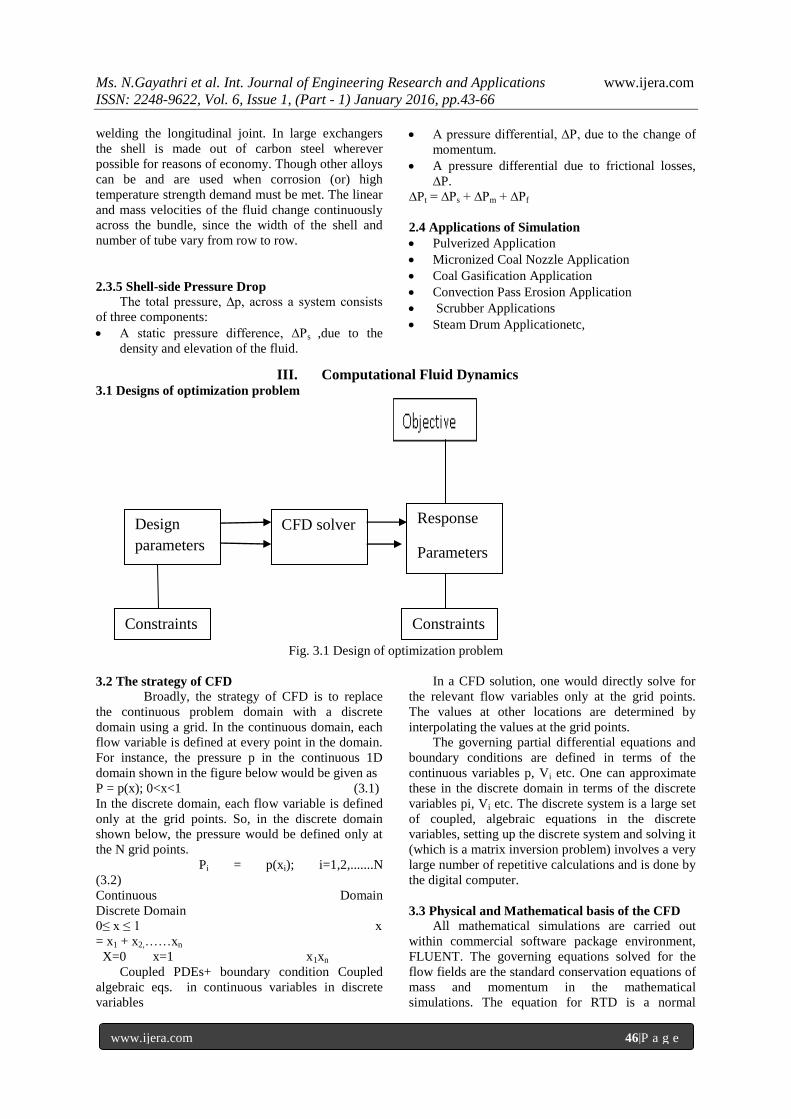
III. Computational Fluid Dynamics 3.1 Designs of optimization problem

Fig. 3.1 Design of optimization problem

3.2 The strategy of CFD

Broadly, the strategy of CFD is to replace

the continuous problem domain with a discrete

domain using a grid. In the continuous domain, each

flow variable is defined at every point in the domain.

For instance, the pressure p in the continuous 1D

domain shown in the figure below would be given as

P = p(x); 0<x<1 (3.1)

In the discrete domain, each flow variable is defined

only at the grid points. So, in the discrete domain

shown below, the pressure would be defined only at

the N grid points.

Pi = p(xi); i=1,2,.......N

(3.2)

Continuous Domain

Discrete Domain

0≤ x ≤ 1 x

= x1 + x2,……xn

X=0 x=1 x1xn

Coupled PDEs+ boundary condition Coupled

algebraic eqs. in continuous variables in discrete

variables

In a CFD solution, one would directly solve for

the relevant flow variables only at the grid points.

The values at other locations are determined by

interpolating the values at the grid points.

The governing partial differential equations and

boundary conditions are defined in terms of the

continuous variables p, Vi etc. One can approximate

these in the discrete domain in terms of the discrete

variables pi, Vi etc. The discrete system is a large set

of coupled, algebraic equations in the discrete

variables, setting up the discrete system and solving it

(which is a matrix inversion problem) involves a very

large number of repetitive calculations and is done by

the digital computer.

3.3 Physical and Mathematical basis of the CFD

All mathematical simulations are carried out

within commercial software package environment,

FLUENT. The governing equations solved for the

flow fields are the standard conservation equations of

mass and momentum in the mathematical

simulations. The equation for RTD is a normal

Design

parameters

CFD solver Response

Parameters

Constraints Constraints




species transportation equation. For trajectories of the

inclusion, discrete phase model (DPM) is employed

with revised wall boundary conditions. The free

surface and tannish walls have different boundary

conditions (such as reflection and entrapment) for

droplets/solid inclusion particles. Taking the range of

inclusion particles‟ diameter (Chevrier and Cramb,

2005) and the shapes for different types of inclusions

(Beskow, et al., 2002) into consideration, the

boundaries and drag law for particles are then revised

by user defined function (UDF) and shape correction

coefficient. During trajectory simulations, Stokes-

Cunningham drag law is employed with Cunningham

correction. Inclusions sometimes could be liquid

phase. It is difficult to set the correction coefficient

(Haider and Leve spiel, 1989) exactly since droplets

can move and deform continuously. While Sinha and

Sahai (1993) set both top free face and walls as trap

boundary, Lopez-Ramirez et al. (2001) did not

illustrate the boundary conditions for inclusion.

Zhang, et al. (2000) divided the tannish into two

kinds of separate zones. The walls are set as

reflection boundary in this work for comparison of

separation ratios of inclusion in SFT and a tundish

with TI. Although most of the reports indicate that

the free surface is a trap boundary, there is a

possibility of re-entrainment (Bouris and Bergeles,

1998) to be considered.

3.4 Fluid Flow Fundamentals

The physical aspects of any fluid flow are

governed by three fundamental principles. Mass is

conserved; Newton‟s second law and Energy is

conserved. These fundamental principles can be

expressed in terms of mathematical equations, which

in their most general form are usually partial

differential equations. Computational Fluid

Dynamics (CFD) is the science of determining a

numerical solution to the governing equations of fluid

flow whilst advancing the solution through space or

time to obtain a numerical description of the

complete flow field of interest.

The governing equations for Newtonian fluid

dynamics, the unsteady Navier-stokes equations,

have been known for over a century. However, the

analytical investigation of reduced forms of these

equations is still an active area of research as is the

problem of turbulent closure for the Reynolds

averaged form of the equations. For non-Newtonian

fluid dynamics, chemical reacting flows and

multiphase flows theoretical developments are at a

less advanced stage.

Experimental fluid dynamics has played an

important role in validating and delineating the limits

of the various approximations to the governing

equations. The wind tunnel, for example, as a piece

of experimental equipment, provides an effective

means of simulating real flows. Traditionally this has

provided a cost effective alternative to full scale

measurement. However, in the design of the

equipment that depends critically on the flow scale

measurement as part of the design process is

economically impractical. This situation has led to an

increasing interest in the development of a numerical

wind tunnel.

3.5 The Governing equations

In the case of steady- two dimensional flow, the

continuity (conservation of mass) equation is: 𝝏 𝝆𝒖

𝝏𝒙+

𝝏 𝝆𝒗

𝝏𝒚= 𝟎 (1)

For incompressible flow, the momentum equations

are the x direction:

𝝆𝒖𝝏𝒖

𝝏𝒙+ 𝝆𝒗

𝝏𝒖

𝝏𝒚= −

𝝏𝝆

𝝏𝒙+

𝝏 𝟐µ𝝏𝒖

𝝏𝒙

𝝏𝒙+

𝝏 µ 𝝏𝒖

𝝏𝒚+

𝝏𝒗

𝝏𝒙

𝝏𝒚(2.a)

And for y direction:

𝝆𝒖𝝏𝒗

𝝏𝒙+ 𝝆𝒗

𝝏𝒗

𝝏𝒚= −

𝝏𝝆

𝝏𝒚− 𝝆𝒈 +

𝝏 µ 𝝏𝒗

𝝏𝒙+

𝝏𝒖

𝝏𝒚

𝝏𝒙+

𝝏 𝟐µ𝝏𝒗

𝝏𝒚

𝝏𝒚,

(2.b) The energy conservation equation for the fluid,

neglecting viscous dissipation and compression

heating, is:

𝝆 𝑪𝒑 𝒖𝝏𝑻

𝝏𝒙+ 𝒗

𝝏𝑻

𝝏𝒚 =

𝝏 𝒌𝝏𝑻

𝝏𝒙

𝝏𝒙+ 𝝏

𝒌𝝏𝑻

𝝏𝒚

𝝏𝒚(3)

The above equations are called Naiver-Stokes.

Andthese are solved using a standard well-verified

discretization technique which in turn forms

algebraic equations. These equations particularly

suited for CFD. The following section illustrates the

discretization techniques.

3.6 Method of solution

Discretization

Explicit and Implicit Schemes

Stability Analysis

Some points to note:

1. CFD codes will allow you to set the

Courant number (which is also referred to as

the CFL number) when using time-stepping.

Taking larger time-steps leads to faster

convergence to the steady state, so it is

advantageous to set the Courant number as

large as possible within the limits of

stability.

2. A lower courant number is required during

start-up when changes in the solution are

highly nonlinear but it can be increased as

the solution progresses.

3. Under- relaxation for non-time stepping.

3.7 Fluent as a modelling and analysis tool

In parallel with the construction of physical

models, a succession of computational fluid

dynamics (CFD) models were developed during the

prototype design phase. The software chosen for

numerical modelling in this project was fluent. The

software was easily learned and very flexible in use.

Boundary conditions could be set up quickly and the




software could rapidly solve problems involving

complex flows ranging from incompressible (low

subsonic) to mildly compressible (Transonic) to

highly compressible (Supersonic) flows. The wealth

of physical models in Fluent allows to accurately

predicting laminar and turbulent flows, various

modes of heat transfer. Chemical reactions,

multiphase flows, and other phenomena with

complete mesh flexibility and solution based mesh

adoption.

The governing partial differential equations

for the conservation of momentum and scalars such

as mass, energy and turbulence are solved in the

integral form. Fluent uses a control-volume based

technique. The governing equations are solved

sequentially. The fact that these equations are

coupled makes it necessary to perform several

iterations of the solution loop before convergence can

be reached. The solution loop consists of seven steps

that are performed in order.

The momentum equations for all directions are

each solved using the current pressure values

(initially the boundary condition is used), in

order to update the velocity field.

The obtained velocities may not satisfy the

continuity equation locally. Using the continuity

equation and the linear zed momentum equation

a „Poisson-type‟ equation for pressure correction

is derived. Using this pressure correction the

pressure and velocities are corrected to achieve

continuity.

K and ε equations are solved with corrected

velocity field.

All other equations (energy, species conservation

etc.) are solved using the corrected values of the

variables.

Fluid properties are updated.

Any additional inter-phase source terms are

updated.

A check for convergences is performed.

These seven steps are continued until in the last

step the convergence criteria are met.

3.8 Imposing Boundary Conditions

The boundary conditions determine the flow and

thermal variables on the boundaries of the physical

model. There are a number of classifications of

boundary conditions:

Flow inlet and exit boundaries: pressure inlet,

velocity inlet, inlet vent, intake fan, pressure

outlet, out flow, outlet fan, and exhaust fan.

Wall, repeating, and pole boundaries: wall,

symmetry, periodic, and axis.

Internal cell zone: fluid, solid.

Internal face boundaries: fan, radiator, porous

jump, wall, interior.

With the determination of the boundary

conditions the physical model has been defined and

numerical solution will be provided.

IV. Modelling of periodic flow using

gambit and fluent 4.1 Introduction

Many industrial applications, such as steam

generation in a boiler, air cooling in the coil of air

conditioner and different type of heat exchangers

uses tube banks to accomplish a desired total heat

transfer.

The system considered for the present problem,

consisted bank of tubes containing a flowing fluid at

one temperature that is immersed in a second fluid in

cross flow at a different temperature. Both fluids are

water, and the flow is classified as laminar and

steady, with a Reynolds number of approximately

100.The mass flow rate of cross flow is known, and

the model is used to predict the flow and temperature

fields that result from convective heat transfer due to

the fluid flowing over tubes.

The figure depicts the frequently used tube banks

in staggered arrangements. The situation is

characterized by repetition of an identical module

shown as transverse tubes. Due to symmetry of the

tube bank, and the periodicity of the flow inherent in

the tube geometry, only a portion of the geometry

will be modelled as two dimensional periods‟ heat

flows with symmetry applied to the outer boundaries.

4.2 CFD modelling of a periodic model

Creating physical domain and meshing

Creating periodic zones

Set the material properties and imposing

boundary conditions

Calculating the solutions using segregated

solver.




Fig. 4.3.1.Schematic diagram of the problem

The modelling and meshing package used is

GAMBIT. The geometry consists of a periodic inlet

and outlet boundaries, tube walls. The bank consists

of uniformly spaced tubes with a diameter D, which

are staggered in the direction of cross flow. Their

centres are separated by a distance of 2cm in x-

direction and 1 cm in y-direction.

The periodic domain shown by dashed lines in

fig 4.3.1.is modelled for different tube diameter viz.,

D=0.8cm, 1.0cm, 1.2cm and 1.4cm while keeping the

same dimensions in the x and y direction. The entire

domain is meshed using a successive ratio scheme

with quadrilateral cells. Then the mesh is exported to

FLUENT where the periodic zones are created as the

inflow boundary is redefined as a periodic zone and

the outer flow boundary defined as its shadow, and to

set physical data, boundary condition. The resulting

mesh for four models is shown in fig 4.3.2

4.3 Modelling details and meshing

Fig. 4.3.2 Mesh for the periodic tube of diameters 0.8, 1.0, 1.2, 1.4cm

4.4 Material properties and boundary conditions

The material properties of working fluid (water)

flowing over tube bank at bulk temperature of 300K,

are:

ρ = 998.2kg/m3

µ = 0.001003kg/m-s

Cp = 4182 J/kg-k

K= 0.6 W/m-k

4.4.1 Boundary conditions assigned in FLUENT




The boundary conditions applied on physical domain

are as follows

Fluid flow is one of the important characteristic of a

tube bank. It is strongly effects the heat transfer

process of a periodic domain and its overall

performance. In this paper, different mass flow rates

at free stream temperature, 300Kwere used and the

wall temperature of the tube which was treated as

heated section was set at 400K as periodic boundary

conditions for each model which are tabulated as

follows

4.4.2 Mass flow rates for different tube diameter

Tube diameter(D)

(cm)

Periodic condition

(Kg/s)

0.8 m=0.05-0.30

1.0 m=0.05,0.30

1.2 m=0.05-0.30

1.4 m=0.05-0.30

The wall temperature of the tube which was treated

as heated section was set at 400k.

4.5 Solution using Segregate Solver

The computational domain was solved using the

solver settings as segregated, implicit, two-

dimensional and steady state condition. The

numerical simulation of the Naiver Stokes equations,

which governs the fluid flow and heat transfer, make

use of the finite control volume method. CFD solved

for temperature, pressure and flow velocity at every

cell. Heat transfer was modelled through the energy

equation. The simulation process was performed until

the convergence and an accurate balance of mass and

energy were achieved. The solution process is

iterative, with each iteration in a steady state

problem. There are two main iteration parameters to

be set before commencing with the simulation. The

under-relaxation factor determines the solution

adjustment for each iteration; the residual cut off

value determines when the iteration process can be

terminated. The under-relaxation factor is an arbitrary

number that determines the solution adjustment

between two iterations, a high factor will result in a

large adjustment and will result in a fast convergence,

if the system is stable. In a less stable or particularly

nonlinear system, for example in some turbulent flow

or high- Rayleigh-number natural convection cases, a

high under-relaxation may lead to divergence, an

incr

ease

in

erro

r. It

is

therefore necessary to adjust the under- relaxation

factor specifically to the system for which a solution

is to be found. Lowering the under-relaxation factor

in these unstable systems will lead to a smaller step

change between the iterations, leading to less

adjustment in each step. This slows down the

iterations process but decreases the chance for

divergence of the residual values.

The second parameter, the residual value,

determines when a solution is converged. The

residual value (a difference between the current and

former solution value) is taken as a measure for

convergence. In a infinite precision process the

residuals will go to zero as the process converges. On

actual computers the residuals decay to a certain

small value (round-off) and then stop changing. This

decay may be up to six orders of magnitude for single

precision computations. By setting the upper limit of

the residual values the „cut-off‟ value for

convergence is set. When the set value is reached the

process is considered to have reached its „round-off‟

value and the iteration process is stopped.

Finally the under-relaxation factors and the

residual cut-off values are set. Under- relaxation

factors were set slightly below their default values to

ensure stable convergence. Residual values were kept

at their default values, 1.0e-6

for the energy residual,

1.0e-3

for all others, continuity, and velocities. The

residual cut-off value for the energy balance is lower

because it tends to be less stable than the other

balances; the lower residual cut-off ensures that the

energy solution has the same accuracy as the other

values.

V. Resulting plots/Graphs & Tables 5.1 Convergence plot for different mass flow rates

with diameter D=0.8cm

Here we are representing the resultant values for

only one diameter i.e; D=0.8cm with different mass

flow rate values (i.e; m=0.05, 0.10, 0.15, 0.20, 0.25,

& 0.30kg/s) we got the other results for other

diameters also but not representing here.

Boundary Assigned as

Inlet Periodic

Outlet Periodic

Tube walls Wall

Outer walls Symmetry




Fig.5.1.1 convergence plot for tube D=0.8cm, m=0.05kg/sFig.5.1.2 D=0.8cm,m=0.10kg/s

Fig.5.1.3 D=0.8cm, m=0.15kg/sFig.5.1.4D=0.8cm,m=0.20kg/s

Fig.5.1.5 D=0.8cm,m=0.25kg/sFig.5.1.6D=0.8cm,m=0.30kg/s

Similarly we got the results for other diameters with the different mass flowrate values

VI. Results through CFD 6.1 Variation of static pressure for different mass flow rates with diameter D=0.8cm

Here we are representing the resultant values for only one diameter i.e; D=0.8cm with different mass flow

rate values (i.e; m=0.05, 0.10, 0.15, 0.20, 0.25, & 0.30kg/s) we got the other results for other diameters also but

not representing here.




Fig. 6.1.1D=0.8cm,m=0.05kg/ Fig.6.1.2 D=0.8cm,m=0.10kg/s

Fig. 6.1.3 D=0.8cm,m=0.15kg/s Fig.6.1.4 D=0.8cm,m=0.20kg/s


6.2 Static Temperature for different mass flow rates with diameter D=0.8cm







Fig.6.2.1 D=0.8cm,m=0.05kg/s Fig.6.2.2.D=0.8cm,m=0.10kg/s


Fig. 6.2.5 D=0.8cm,m=0.25kg/ Fig.6.2.6 D=0.8cm,m=0.30kg/s

6.3.1 Velocity vector for different mass flow rates with diameter D=0.8cm







Fig.6.3.1 D=0.8cm,m=0.05kg/s Fig.6.3.2.D=0.8cm,m=0.10kg/s

Fig.6.3.3.D=0.8cm,m=0.15kg/s Fig.6.3.4.D=0.8cm,m=0.20kg/s


6.4 Static Pressure for different mass flow rates with diameter D=0.8cm










6.5 Static temperature variation in y-axis for different mass flow rates with diameter D=0.8cm









Fig.6.5.5.D=0.8cm,m=0.25kg/s Fig.6.5.6D=0.8cm,m=0.30kg/s




6.6 Static Pressure Variation in y-axis for different mass flow rates with diameter D=0.8cm







6.7 Nusselt number plot with different mass flow rates with diameter D=0.8cm







Fig.6.7.1.D=0.8cm,m=0.05kg/s Fig.6.7.2D=0.8cm,m=0.10kg/s






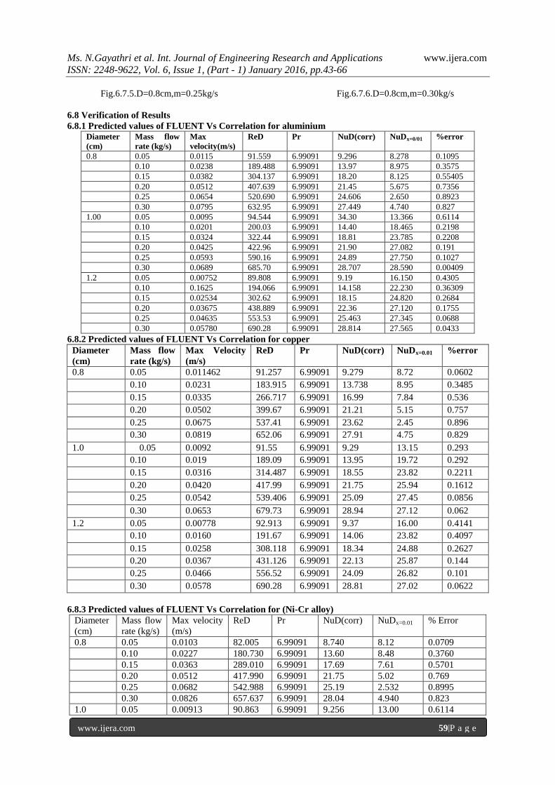
6.8 Verification of Results

6.8.1 Predicted values of FLUENT Vs Correlation for aluminium

Diameter

(cm)

Mass flow

rate (kg/s)

Max

velocity(m/s)

ReD Pr NuD(corr) NuDx=0/01 %error

0.8 0.05 0.0115 91.559 6.99091 9.296 8.278 0.1095

0.10 0.0238 189.488 6.99091 13.97 8.975 0.3575

0.15 0.0382 304.137 6.99091 18.20 8.125 0.55405

0.20 0.0512 407.639 6.99091 21.45 5.675 0.7356

0.25 0.0654 520.690 6.99091 24.606 2.650 0.8923

0.30 0.0795 632.95 6.99091 27.449 4.740 0.827

1.00 0.05 0.0095 94.544 6.99091 34.30 13.366 0.6114

0.10 0.0201 200.03 6.99091 14.40 18.465 0.2198

0.15 0.0324 322.44 6.99091 18.81 23.785 0.2208

0.20 0.0425 422.96 6.99091 21.90 27.082 0.191

0.25 0.0593 590.16 6.99091 24.89 27.750 0.1027

0.30 0.0689 685.70 6.99091 28.707 28.590 0.00409

1.2 0.05 0.00752 89.808 6.99091 9.19 16.150 0.4305

0.10 0.1625 194.066 6.99091 14.158 22.230 0.36309

0.15 0.02534 302.62 6.99091 18.15 24.820 0.2684

0.20 0.03675 438.889 6.99091 22.36 27.120 0.1755

0.25 0.04635 553.53 6.99091 25.463 27.345 0.0688

0.30 0.05780 690.28 6.99091 28.814 27.565 0.0433

6.8.2 Predicted values of FLUENT Vs Correlation for copper

Diameter

(cm)

Mass flow

rate (kg/s)

Max Velocity

(m/s)

ReD Pr NuD(corr) NuDx=0.01 %error

0.8 0.05 0.011462 91.257 6.99091 9.279 8.72 0.0602

0.10 0.0231 183.915 6.99091 13.738 8.95 0.3485

0.15 0.0335 266.717 6.99091 16.99 7.84 0.536

0.20 0.0502 399.67 6.99091 21.21 5.15 0.757

0.25 0.0675 537.41 6.99091 23.62 2.45 0.896

0.30 0.0819 652.06 6.99091 27.91 4.75 0.829

1.0 0.05 0.0092 91.55 6.99091 9.29 13.15 0.293

0.10 0.019 189.09 6.99091 13.95 19.72 0.292

0.15 0.0316 314.487 6.99091 18.55 23.82 0.2211

0.20 0.0420 417.99 6.99091 21.75 25.94 0.1612

0.25 0.0542 539.406 6.99091 25.09 27.45 0.0856

0.30 0.0653 679.73 6.99091 28.94 27.12 0.062

1.2 0.05 0.00778 92.913 6.99091 9.37 16.00 0.4141

0.10 0.0160 191.67 6.99091 14.06 23.82 0.4097

0.15 0.0258 308.118 6.99091 18.34 24.88 0.2627

0.20 0.0367 431.126 6.99091 22.13 25.87 0.144

0.25 0.0466 556.52 6.99091 24.09 26.82 0.101

0.30 0.0578 690.28 6.99091 28.81 27.02 0.0622

6.8.3 Predicted values of FLUENT Vs Correlation for (Ni-Cr alloy)

Diameter

(cm)

Mass flow

rate (kg/s)

Max velocity

(m/s)

ReD Pr NuD(corr) NuDx=0.01 % Error

0.8 0.05 0.0103 82.005 6.99091 8.740 8.12 0.0709

0.10 0.0227 180.730 6.99091 13.60 8.48 0.3760

0.15 0.0363 289.010 6.99091 17.69 7.61 0.5701

0.20 0.0512 417.990 6.99091 21.75 5.02 0.769

0.25 0.0682 542.988 6.99091 25.19 2.532 0.8995

0.30 0.0826 657.637 6.99091 28.04 4.940 0.823

1.0 0.05 0.00913 90.863 6.99091 9.256 13.00 0.6114




0.10 0.0199 198.04 6.99091 14.32 18.245 0.2151

0.15 0.0327 325.43 6.99091 17.45 23.567 0.2592

0.20 0.0432 429.93 6.99091 22.10 27.254 0.1889

0.25 0.0515 512.53 6.99091 24.36 27.89 0.1256

0.30 0.0599 596.133 6.99091 26.543 28.674 0.0743

1.2 0.05 0.00783 93.510 6.99091 9.406 14.150 0.335

1.00 0.01656 197.768 6.99091 14.309 19.532 0.267

0.15 0.02534 302.62 6.99091 18.15 24.820 0.2684

0.20 0.0383 457.400 6.99091 22.88 27.12 0.156

0.25 0.0498 594.74 6.99091 26.508 28.645 0.0746

0.30 0.05245 626.86 6.99091 27.289 29.565 0.67769

For better understanding of theoretical values and simulation values for different diameters and mass flow

rates, the following graphs are drawn.

Figure 6.8.1 mass flow rates VsNusselt number for Aluminium tubes

0

5

10

15

20

25

30

35

40

0.05 0.1 0.15 0.2 0.25 0.3

Nu

ssel

t n

um

ber

corr

elati

on

mass flow rates (kg/s)

diamter 0.8

diameter 1.0

diameter 1.2




Figure 6.8.2 mass flow rate Vs Nusselt number for copper tubes.

Figure 6.8.3mass flow rate Vs Nusselt number correlation for Nickel-Chromium base super alloy base tube.

0

5

10

15

20

25

30

35

0.05 0.1 0.15 0.2 0.25 0.3

Nu

ssel

t n

um

ber

corr

elati

on


diameter 0.8

diameter 1.0

diameter 1.2

0

5

10

15

20

25

30

0.05 0.1 0.15 0.2 0.25 0.3

nu

ssel

t n

um

ber

corr

elati

on

e


diameter 0.8

diameter 1.0

diameter 1.2




Figure 6.8.4 mass flow rate Vs Nusselt number theoretical for aluminium

Figure 6.8.5 mass flow rates Vs Nusselt number theoretical for copper tubes.

0

5

10

15

20

25

30

0.05 0.1 0.15 0.2 0.25 0.3

Nu

ssel

t n

um

ber

th

eore

tica

l

mass fow rates (kg/s)

dimater -.8

diameter 1.0

diameter 1.2

0

5

10

15

20

25

30

0.05 0.1 0.15 0.2 0.25 0.3

nu

ssel

t n

um

ber

th

eore

tica

l


diameter 0.8

diameter 1.0

diameter 1.2




Figure 6.8.6 mass flow rates Vs Nusselt number theoretical for Nickel- chromium base super alloy.

Figure 6.8.7 mass flow Vs Nusselt number for different materials at d=0.08cm

0

5

10

15

20

25

30

35

0.05 0.1 0.15 0.2 0.25 0.3

nu

ssel

t n

um

ber

th

eore

tica

l


diameter 0.8

diameter 1.0

diameter 1.2

0

5

10

15

20

25

30

0.05 0.1 0.15 0.2 0.25 0.3

Nu

ssel

t n

um

ber


aluminium

copper

Ni-Cr alloy




Figure 6.8.8 mass flow rates Vs Nusselt number for different materials at d=1.0cm

Figure 6.8.9 mass flow rates Vs mass flow rates for different materials at d=1.20cm

From the above graphs the observations are:

The effect of different mass flow rates on both

flow and heat transfer is significant. It was

observed that 1.0cm diameter of tubes and

0.05kg/s mass flow gives the best results as

34.30 Nusselt number.

From the above graphs we can observe that

alloys serves as a better material for tube when

compare with copper and aluminium.

The effect of mass flow rates on both flow and

heat transfer is significant. This is due to

variation of space of the surrounding tubes.

It was observed optimal flow distribution was

found for 0.8cm diameter and 0.05kg/s mass

flow rate in case of alloy.

VII. Conclusions

0

5

10

15

20

25

30

35

40

0.05 0.1 0.15 0.2 0.25 0.3

nu

ssel

t n

um

ber

mass flow rates kg/s

aluminium

copper

Ni-Cr alloy

0

5

10

15

20

25

30

35

0.05 0.1 0.15 0.2 0.25 0.3

nu

ssel

tn

um

ber


aluminium

copper

Ni-Cr alloy




Mode and mesh creation n CFD is one of the

most important phases of simulation. The model and

mesh density determine the accuracy and flexibility

of the simulations. Too dense a mesh will

unnecessarily increase the solution time; too coarse a

mesh will reach to a divergent solution quickly. But

will not show an accurate flow profile. An optimal

mesh is denser in areas where there are no flow

profile changes.

A two- dimensional numerical solution of flow

and heat transfer in a bank of tubes which is used

in industrial applications has been carried out.

Laminar flow past a tube bank is numerically

simulated in the low Reynolds number regime.

Velocity vector depicts zones of recirculation

between the tubes. Nusselt number variations are

obtained and pressure distribution along the

bundle cross section is presented.

The effect of different mass flow rates on both

flow and heat transfer is significant. This is due

to the variation of space of the succeeding rows

of tubes. It was observed that 1.0cm diameter of

tubes and 0.05kg/s mass flow rate gives the best

results.

Mass flow rate has an important effect to heat

transfer. An optimal flow distribution can result

in a higher temperature distribution and low

pressure drop. It was observed that the optimal

flow distribution was occurred in 1.0cm diameter

and 0.05kg/s mass flow rate.

CFD simulations are a useful tool for

understanding flow and heat transfer principles

as well as for modelling these types of

geometries.

It was observed that 1.0cm diameter of tubes and

0.30kg/s mass flow rate yields optimum results

for aluminium as tube material, where as it was

observed that 0.8cm and 0.05kg/s mass flow rate

in case of copperas tube material.

From the above graphs we observed that alloys

serves as a better material for tube compared

with copper and aluminium.

Alloy (Nickel-Chromium based) serves as a

better material for heat transfer applications with

low cost

Further improvements of heat transfer and fluid

flow modelling can be possible by modelling

three dimensional models and changing the

working fluid.

It was observed that Heat transfer rate is more

for Nano fluids when compared to water.

References [1.] Patankar, S.V. and spalding. D.B. (1974), “

A calculation for the transient and steady

state behaviour of shell- and- tube Heat

Exchanger”. Heat transfer design and theory

sourcebook. Afgan A.A. and SchlunerE.U..

Washington. Pp. 155-176.

[2.] KelKar, K.M and Patankar, S. V., 1987”

Numerical prediction of flow and Heat

transfer in a parallel plate channel with

staggered fins”, Journal of Heat Transfer,

vol. 109, pp 25-30.

[3.] Berner, C., Durst, F. And McEligot, D.M.,

“Flow around Baffles”, Journal of Heat

Transfer, vol. 106 pp 743-749.

[4.] Popiel, C.o& Vander Merwe, D.F., “Friction

factor in sine-pipe flow, Journal of fluids

Engineering”, 118, 1996, 341-345.

[5.] Popiel, C.O &Wojkowiak, J., “friction factor

in U-type undulated pipe flow, Journal of

fluids Engineering”, 122, 2000, 260-263.

[6.] Dean, W. R., Note on the motion of fluid in

a curved pipe, The London, Edinburgh and

Dublin philosophical Magazine, 7 (14),

1927, 208-223.

[7.] Patankar, S.V., Liu, C.H & Sparrow, E.M.,

“Fully developed flow and Heat Transfer in

ducts having streamwise periodic variation

in cross-sectional area”, Journal of Heat

Transfer, 99, 1977, 180-186.

[8.] Webb, B.W &Ramdhyani, S., “Conjugate

Heat Transfer in an channel with staggered

Ribs” Int. Journal of Heat and Mass Transfer

28(9), 1985,1679-1687.

[9.] Park, K., Choi, D-H & Lee, K-s., “design

optimization of plate heat exchanger with

staggered pins”, 14th

Int. Symp.on Transport

phenomena, Bali, Indonesia, 6-9 July 2003.

[10.] N.R. Rosaguti, D.F. Fletcher & B.S. Haynes

“Laminar flow in a periodic serpentine”. 15th

Australasian fluid mechanics conference.

The University of Sydney, Sydney,

Australia 13-17 December 2004.

[11.] L.C Demartini, H.A. Vielmo, S.V. Moller

“Numeric and experimental analysis of

turbulent flow through a channel with baffle

plates”, J. Braz. Soc. Mech.Sci& Eng. Vol

26 No.2 Rio de Janeiro Apr/June 2004.

[12.] Baier, G., Grateful, T.M. Graham, M.D. &

Lightfoot E.N.(1999), “ Prediction of mass

transfer rates in spatially periodic flow”,

Chem. Eng. Sci., 54,343-355.

[13.] Bao, L. & Lipscomb, G.G., 2002 “ Well-

developed mass transfer in axial flows

through randomly packed fiber bundles with

constant wall flux”, Chem. Eng. Sci., 57,

125-132.

[14.] Launder, B.E. & Massey, T.H 1978 “The

numerical predictions of viscous flow and

heat transfer in tubefer bank”. J. Heat

transfer, 100, 565-571.

[15.] Wung, T.S. & Chen, C.J. (1989), “Finite

analytic solution of convective Heat transfer




for tube arrays in cross flow: part- I flow

field analysis”, ASME J. Heat Transfer, 111,

633-640.

[16.] Schoner, P., Plucinski, W.N. &Daiminger,

U. (1998), “Mass transfer in the shell side of

cross flow hollow fiber modules”, Chem.

Eng. Sci. 53, 2319-2326.

[17.] T.Li, N.G. Deen & J.A D.G. M. Kuipers,

faculty of Sci. & Tech, University of

Twente, “Numerical study of

Hydrodynamics and mass transfer of in line

fiber arrays in laminar cross flow”, 3rd

International conference on CFD in the

Minerals and process Industries CSIRO,

Melbourne, Australia 10-12 December 2003,

pg, 87-92.

[18.] T.V. Mull, Jr., M.W. Hopkins and D.G.

White “Numerical Simulation Models for a

Modern Boiler Design “, Power-Gen

International‟ 96, December 4-6, 1996,

Orlando, Florida, U.S.A

[19.] "Enhancing the efficiency of polymerase

chain reaction using graphene Nano flakes -

Abstract- Nanotechnology -

IOPscience" iop.org. Retrieved 8 June 2015.

[20.] "Light: Science & Applications - Abstract of

article: Nano fluid-based optical filter

optimization for PV/T systems". nature.com.

Retrieved 8 June 2015.

[21.] ShimaP.D.and J. Philip (2011). "Tuning of

Thermal Conductivity and Rheology of Nano

fluids using an External Stimulus". J. Phys.

Chem. C 115: 20097–

20104. doi:10.1021/jp204827q.

[22.] "A review on preparation methods and

challenges of Nano

fluids". Sciencedirect.com. Retrieved 8

June 2015.

[23.] Chung, Y.M., Tucker, P.G., “Assessment of

periodic flow assessment for unsteady state

Heat Transfer in grooved channels;

Transaction of the ASME, Vol.126, Dec

(2004).

http://www.nature.com/lsa/journal/v1/n10/abs/lsa201234a.html



https://en.wikipedia.org/wiki/Digital_object_identifier

https://dx.doi.org/10.1021%2Fjp204827q

http://www.sciencedirect.com/science/article/pii/S0735193314000736



heat transfer & periodic flow analysis of heat exchanger by cfd with nano fluids

Documents