heat transfer enhancement in nano-fluids suspensions
TRANSCRIPT

HEAT TRANSFER ENHANCEMENT IN NANO-FLUIDS
SUSPENSIONS: THERMAL WAVE EFFECTS AND
HYPERBOLIC HEAT CONDUCTION
by
Johnathan J. Vadasz
Supervisor: Professor Saneshan Govender
In fulfillment of the requirements for the degree of Master of Science in
Mechanical Engineering at University of KwaZulu-Natal
December 2005
I
Acknowledgements
I would like to thank Professor Saneshan Govender as my supervisor for assistance
in my Masters thesis research. Specifically for supplying me with some Journal
paper publications and other relevant literature to my research. I also thank Professor
Peter Vadas z for many more Journal paper publications and help in the literature
survey, and for assistance in learning FORTRAN programming.
II

ABSTRACT
The spectacular heat transfer enhancement revealed experimentally in nanofluids
suspensions is being investigated theoretically at the macro-scale level aiming at
explaining the possible mechanisms that lead to such impressive experimental
results. In particular, the possibility that thermal wave effects via hyperbolic heat
conduction could have been the source of the excessively improved effective thermal
conductivity of the suspension is shown to provide a viable explanation although the
investigation of alternative possibilities is needed prior to reaching an ultimate
conclusion.
KEYWORDS: Nanofluids, Nanoparticles Suspension, Heat Transfer Enhancement,
Effective Thermal Conductivity.
III

TABLE OF CONTENTS
page
ABSRACT III
NOMENCLATURE VII
1. Introduction
1.1 Motivation 1
1.2 Potential Applications 3
2. Literature Survey 4
2.1 Heat Transfer Enhancement in Nanofluids Suspensions 4
2.2 Transient Hot Wire and Transient Hot Strip Methods of Measuring
the Thermal Conductivity 9
2.3 Hyperbolic Heat Conduction and Thermal Wave Effects 14
3. Problem Formulation 16
3.1 Fourier and Hyperbolic Heat Conduction in rectangular geometry. 16
3.1.1 Fourier heat conduction with Dirichlet boundary conditions 16
3.1.2 Fourier heat conduction with Dirichlet-Neumann boundary
conditions 18
3.1.3 Hyperbolic heat conduction with Dirichlet boundary
conditions 18
3.1.4 Hyperbolic heat conduction with Dirichlet-Neumann
boundary conditions 19
3.2 Fourier and Hyperbolic Heat Conduction in cylindrical geometry. 22
3.2.1 Fourier heat conduction with Dirichlet-Neumann boundary
conditions 22
3.2.2 Hyperbolic heat conduction with Dirichlet-Neumann boundary
conditions 23
4. Solution to the Heat Conduction Problem 26
4.1 Solution to the Heat Conduction Problem in rectangular geometry 26
4.1.1 Solution to the Fourier Heat conduction Problem subject to
Dirichlet boundary conditions. 26
IV

4.1.2 Solution to the Fourier Heat conduction Problem subject
to a combination of Dirichlet and Neumann boundary
conditions. 27
4.1.3 Solution to the Hyperbolic Heat Conduction Problem subject
to Dirichlet boundary conditions. 28
4.1.4 The time needed for a pulse to cross the gap in rectangular
geometry. 31
4.1.5 Solution to the Hyperbolic Heat Conduction Problem subject
to a combination of Dirichlet and Neumann boundary
conditions. 32
4.2 Solution to the Heat Conduction Problem in cylindrical geometry 35
4.2.1 Solution to the Fourier Heat conduction Problem subject
to a combination of Dirichlet and Neumann boundary
conditions. 35
4.2.2 Solution to the Hyperbolic Heat Conduction Problem subject
to a combination of Dirichlet and Neumann boundary
conditions. 36
4.2.3 The time needed for a pulse to cross the gap in cylindrical
geometry. 38
5. Results and Discussion 39
5.1 Analytical solution evaluated using Fortran. 39
5.2 Results for the Fourier Heat Conduction Problem subject to
Dirichlet boundary conditions . 40
5.3 Results for the Fourier Heat Conduction Problem subject to a
combination of Dirichlet and Neumann boundary conditions. 42
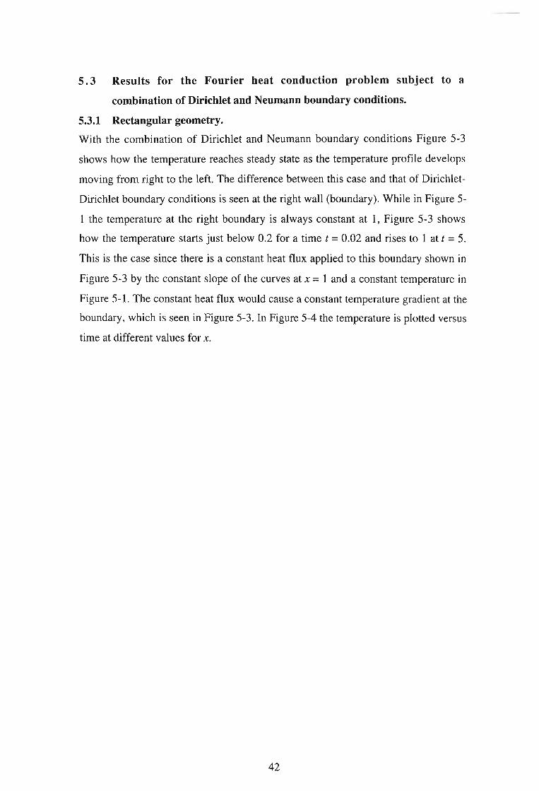
5.3.1 Rectangular geometry. 42
5.3.2 Cylindrical geometry. 45
5.4 Results for the Hyperbolic Heat Conduction Problem subject to
Dirichlet boundary conditions in rectangular geometry. 48
v

5.5 Results for the Hyperbolic Heat Conduction Problem subject to a
combination of Dirichlet and Neumann boundary conditions. 70
5.5.1 Rectangular geometry. 70
5.5.2 Cylindrical geometry. 87
5.6 Results of the SEED (Synthetic Experimental Emulation Data)
method. 108
6. Conclusions 136
APPENDICES 137
Appendix A 137
REFERENCES 139
VI

NOMENCLATURE
Latin Symbols
rw• = radius of the platinum wire .
c. = wave speed, equals ~a./T• .
dw• = diameter of the platinum wire.
Fo = Fourier number, equalsrz.r.j' L: .
i = electrical current.
k: = effective thermal conductivity of the suspension.
l, = length of the platinum wire/strip.
L = gap distance between the walls of a slab.
q. = heat flux.
qL' = horizontal heat flux on the boundary of the platinum strip, at x, = L• .
o., = rate of heat generated by Joule heating in the platinum wire per unit length of
wtre.
R = electrical resistance, dimensional.
r, = radial variable coordinate.
t; = time.
T = dimensionless temperature.
Te•= coldest wall temperature, dimensional.
T•• = temperature measured at time t., .
T2• = temperature measured at time t.2 •
V = voltage across the platinum wire/strip, dimensional.
x, = horizontal variable co-ordinate.
0= order of
Greek Symbols
a. = effective thermal diffusivity of the suspension.
T. = relaxation time in hyperbolic heat conduction.
p = fluid density.
e= angle between vector V and VT
VII

y = Euler's constant.
A= Eigenvalues
8 = Kronecker delta function
Subscripts
* = dimensional values.
cr =critical values.
VIII

CHAPTERl
INTRODUCTION
1.1 Motivation
Heat conduction in fluids at the macro-level is very poor because most affordable
fluids have very low thermal conduct ivity values compared with solids . Crystalline
solids have thermal conductivity values of 1 to 3 orders of magnitude larger than
those of fluids (Eastman et al. , 2001).
Traditional enhancement of heat transfer in fluids is possible mainly by adding a
mechanism of convection to the thermal conduction process. Unfortunately, in
addition to the relatively low thermal conductivity of fluids, the convection effect
requires substantial amount of pumping power. The reason for the latter is that the
heat transfer by convection is governed by the energy equation that can be presented
in the following form
aT 2- + v .VT = a V T (1-1)atwhere T stands for temperature, V is the velocity field , a = k/ p Cp is the thermal
diffusivity, k is the thermal conductivity , p is fluid's density, and cp is the specific
heat at constant pressure. From equation (1-1) it is obvious that when the fluid flow
is perpendicular to the temperature gradient the convection term vanishes identically,
i.e. V. VT = 0 when V is perpendicular to VT . The latter occurs because
IV •VT I= IV II VT Icos(e), where e is the angle between the velocity vector
direction and the temperature gradient direction. When they are perpendicular,
e=n12, and the scalar product vanishes . However, according to Fourier law the
temperature gradient is proportional to the heat flux, i.e. q = -kVT , where q is the
heat flux. Therefore, the obvious conclusion is that whenever the heat flux is
perpendicular to the velocity, the convection mechanism vanishes and the heat is
transferred by conduction only. It is because of this reason that most convection
driven devices use one of the two following methods to enhance the convection
mechanism:
(a) Classical/traditional method: "brute force" - apply very high flow rates and
additional means to guarantee that the flow is in the turbulent regime (high Reynolds
1
number) and as a result of the temporal and spatial velocity fluctuations within the
turbulent regime preventing the velocity to be perpendicular to the heat flux. The
price of applying this method is the substantial pumping power required to keep the
flow within the turbulent regime.
(b) Modem methods: elegant design of compact heat exchangers attempt to control
boundary layers by focusing on shape changes of the solid-fluid interface (that acts
as the heat transfer area). While the latter method is indeed more efficient it is
limited in the amount of heat that can be removed and it also requires substantial
pumping power (although less than the former) to overcome the friction due to
enhanced heat transfer area.
Pumping power is a substantially more expensive commodity than the corresponding
energy in the form of heat rate. Thermodynamically, the value of mechanical energy
transfer (pumping power) is between 2 to 3 times more expensive (in terms of
thermodynamic cost) than the same energy amount in the form of heat transfer. For
example 1 kW of heat transferred is equivalent to between 0.35 - 0.5 kW of
mechanical (pumping) power. The latter is a consequence of the second law of
thermodynamics linked with practical state of the art efficiencies related to available
technologies. This makes savings in pumping power while providing the same
amount of heat transfer rates an important engineering objective that holds potential
for great returns.
The reported breakthrough in substantially increasing the thermal conductivity of
fluids by adding very small amounts of suspended metallic or metallic oxide
nanoparticles (Cu, CuO, A120 3) to the fluid (Eastman et at. 2001, Lee et at. 1999), or
alternatively using nanotube suspensions (Choi et at. 2001), as well as Xuan and Li
(2000) is intriguing. The latter is important not only because of the face value of its
possibility to direct implementation in technological applications but also because
both results clearly conflict with theoretical anticipations based on existing theories
and models (see discussion on the conflict between theory and experiments in Choi
et at. 2001). These results, if independently confirmed, open two distinct avenues of
opportunities: (a) Their direct application to different technologies in improving
substantially the operating efficiencies and reducing both operating as well as capital
production costs. Better efficiency allows for lower pumping power and less heat
transfer area, hence saving in both operating as well as fixed costs. Better efficiency
2

also minimizes the adverse impact that energy-producing technologies have on the
environment, i.e. less pollutants per kW generated. (b) By discovering the correct
mechanism and theory that underlies this phenomenon may extend design options in
developing processes and devices that apply these mechanisms, hence opening the
door to yet unknown and limitless possibilities of new processes and devices that use
heat transfer.
1.2 Potential applications
There is a vast field for applications of nano-fluid suspensions. One such application
is in the motor and trucking industry. Recent experiments yielded an increase in
thermal conductivity when suspending nano-copper particles in oil and ethylene
glycol (anti-freeze). This would allow for great savings in the trucking industry by
increasing the efficiency of the engine cooling system. By increasing the thermal
conductivity the heat from the engine would be drawn away more efficiently. This
would allow for reduced fuel consumption, which equals large economical savings
for truck companies. As far as passenger vehicles are concerned, sales would
increase if new cars were to come with a substantially lower fuel consumption index.
Other possible applications include aeronautics, power generation, cooling of
microelectronics etc. The limits are virtually endless when it comes to where nano
fluid suspensions can be used.
3
CHAPTER 2
LITERATURE SURVEY
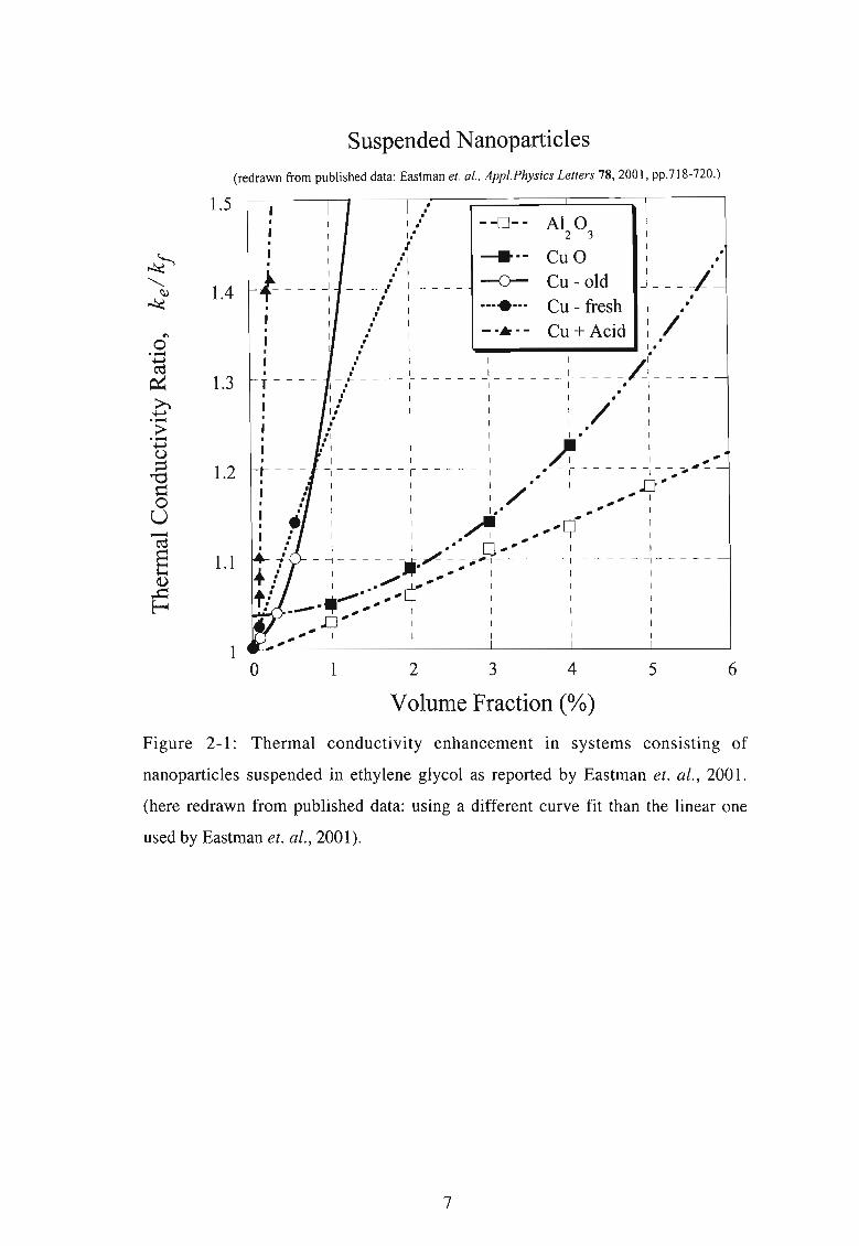
2.1 Heat transfer enhancementin Nano-fluids suspensions
The results reported by Eastman et al. 2001 for a "suspended nano-particles " system
were redrawn and are presented in Figure 2-1 where two major deductions can be
made: (a) The impact of the copper nano-particles (that the authors , Eastman et. ai.
2001 succeeded to keep stable in the suspension due to the particular technique they
used to manufacture them) on the effective thermal conductivity of the suspension is
unexpectedly high. A very small amount (less than 1% in terms of volume fraction)
of copper nano-particles can improve the thermal conductivity of the suspension by
40%. (b) Even metal-oxides at small quantities (4% in terms of volume fraction) can
produce a substantial increase of about 20% in the effective thermal conductivity of
the suspension.
The experimental results reported by Choi et. al. (2001) of multiwalled carbon nano
tubes suspended in oil were redrawn and are presented in Figure 2-2. An even more
impressive improvement of the effective thermal conductivity is detected. Over
150% improvement of the effective thermal conductivity (a factor of 2.5 higher
thermal conductivity) at a volume fraction of 1% is indeed spectacular.
Moreover, Choi et ai. (2001) compared their results with exiting theories , some of
them going back to the start of the last century , e.g. Maxwell (1904), Hamilton &
Crosser (1962), Jeffrey (1973), Davis (1986), Lu & Lin (1996) and Bonnecaze &
Brady (1990, 1991). The reported experimental results are by one order of magnitude
greater than the predictions based on existing theories and models. More recent
approaches (Wang, Zhou and Peng 2003) also cannot explain this discrepancy.
On the other hand a reduction in the effective thermal conductivity of the
nanoparticle-host medium is anticipated by existing theories for length scales smaller
than the phonon mean free path in the host material (Chen, 1996, 2000). There is a
clear and appealing need to settle the conflict between the recent experimental results
and the theories or models . It is very difficult and expensive to experiment for all
possible combinations of circumstances. It is because of this latter reason that
reliable theories and models can be used to bridge the gap between different
experiments. Possible explanations for the divergence between theory and
4

experiments were suggested and explored very basically by Keblinski et al. (2002) .
Brownian motion of the particles, molecular-level layering of the liquid at the
liquid/particle interface, the nature of heat transport within the nanoparticles and
effects of nanoparticle clustering were investigated. While these investigations were
not done in detail but mainly at the very basic level, Keblinski et al. (2002) show that
the "key factors in understanding thermal properties of nanofluids are the ballistic,
rather than diffusive, nature of heat transport in the nanoparticles, combined with
direct or fluid mediated clustering effects that provide paths for rapid heat transport".
If this conclusion is correct then the experimental results obtained at the macro
system level reflect the wave effects impact on the macro-system behavior rather
than the diffusion mechanism. It implies that Fourier Law (representing the diffusion
mechanism) is not valid even at the macro-system level when nanoelements are
suspended in the fluid. The immediate conclusion from the latter deduction is that the
Transient Hot Wire method (THW) that was used by Eastman et al. (2001), Lee et al.
(1999) and by Choi et al. (2001) to measure the nano-fluid suspension's effective
thermal conductivity is not appropriate because it uses the Fourier Law of heat
conduction as its fundamental principle for estimating the thermal conductivity
(Kestin and Wakeham 1978, Perkins et al. 2000). Eastman et ai. (2001) indicate the
way the thermal conductivity is being evaluated by using Fourier Law in the
Transient Hot Wire method (THW). Therefore, based on this simple logic the
excessive values of effective thermal conductivity calculated based on the
experimental data might need a correction to account for deviations from Fourier
Law. Still the question of why this apparent substantial heat flux enhancement
occurred was not yet addressed. The mechanisms suggested by Keblinski et al.
(2002) are all possible. However, the way these nano or molecular level mechanisms
are being lumped into such an impressive effect at the macro-system level is not yet
known, nor proposed by Keblinski et al. (2002). Recent research results presented by
Xue et al. (2004) eliminate the molecular-level layering of the liquid at the
liquid/particle interface as a possible heat transfer enhancement mechanism. The
authors Xue et al. (2004) conclude that "the experimentally observed large
enhancement of thermal conductivity in suspensions of solid nanosized particles
(nanofluids) can not be explained by altered thermal transport properties of the
layered liquid". While the reported results are a direct consequence of the presence
5

of nano-elements in the suspension, the measurements were not performed at the
nanoscale, but rather at the macro/meso-scale. As a result the interest should be
focused not only on what occurs at the nanoscale but rather on how the heat transfer
at the macro/meso-scale is substantially affected by a very small presence (less than
1% in volume) of extremely small suspended elements (nano-elements).
There are about six possible reasons for the anomalously increased effective thermal
conductivity, which can be classified as follows:
(i) Hyperbolic (Cattaneo, 1958 and Vernotte 1958, 1961) or Dual-Phase
Lagging (Tzou 1997, 2001 and Vadasz 2005 a,b) thermal wave effects not accounted
for in using the THW data processing & extremely high values of the time lag due to
the heterogeneous mixture (see Vadasz 2005 a,b),
(ii) Thermal resonance due to hyperbolic thermal waves combined with an
amplified periodic signal possibly from short-radio-waves or cellular phones (1.9
Ghz, 800Mhz frequencies),
(iii) Particle driven, or thermally driven, natural convection,
(iv) Convection induced by electro-phoresis,
(v) Hyperbolic thermal natural convection,
(vi) Any combination of the above.
The first particular possibility that needs exploration is that the nano/molecular level
wave effects at the nanoelements' interface make the hyperbolic (wave) heat transfer
effects at the macro-level significant. Then, a corresponding correction of converting
the experimental data into the effective thermal conductivity results needs to be
introduced. The latter forms the objective of the present investigation in terms of
introducing the hyperbolic thermal wave corrections based on Cattaneo (1958) and
Vernotte (1958, 1961) constitutive relationship for heat conduction and checking
whether such effects may have been the reason behind the excessive effective
thermal conductivity results in nanofluid suspensions.
6
Suspended Nanoparticles
(redrawn from published data: Eastman et. 01., Appl.Physics Letters 78, 2001, pp.718-nO.)
65234
Volume Fraction (%)
1
,..1 .. - -0- - Al 0 1
I: 2 3 IJ 1
/ 1 ---.- Cu 0 1_ __ ./~ ~ _ _ _ _ -0- Cu - old _: - - - -I'
, 1 1 ,... I ••••••• Cu - fresh 1 "
: I I /: 1 - ..... - Cu + Acid 1, '
• I I •, ,
r - - - - 1 - ,/- - - - ~ - - - - - - : - - - - - - ~ - - - -,~: - - - - -, ,
I .. I 1 I' I
I : 1 I 1 / 1:" 1 1 1 1
: 1 1 1 1 , I
: 1 1 1 .. 1
I I 1 /1 I , '~ - -- - --r - - - -- ~ - - - ~ r - r- - - -- ~ - ~~ - -
I I I ' 1 LJ "1 1 I / I ", 1I I I . - I .. I
I I ~ , n' I1 1 ./1 , .. ' I' 1
I I . - 0""- 1 I- ~ - - - - - -JJ.~ : ; ..~ - - - - - - ~ - - - - - -:- - - - -1 ••• / ,..1.," 1 I 1
•......... ,'U 1 I 1
......... ...,~- I I I I
l]' 1 I 1 I
1 1 I 1 1
.~- -- - -:
I·I·I·r - - -·I
o1
1.1
1.2
1.3
1.4
1.5
Figure 2-1: Thermal conductivity enhancement in systems consisting of
nanoparticles suspended in ethylene glycol as reported by Eastman et. al., 2001.
(here redrawn from published data: using a different curve fit than the linear one
used by Eastman et. al., 2001).
7

Suspended Nanotubes(redrawn from published data: Choi et. al., Appl.Phys ics Letters 79, 2001, pp2252-2254 .)
1.20.80.60.40.2
1
I .......· Thermal Conductivity Ratio I :I Ii i1 1 1 1 I_
- - - - - ~ - - - - - ~ - - - - - - r - - - - - - I - - - - - - . ' - - - - -
1 1 I . ' 1.1 1 I .'I I I ...
1 1 1 .'1 1 I .'
I I .'__ _ __ L J ~~ - - - - - - L - - - - -
I I ••- I II I .- I 1I I ••• I I
1 1 ." 1 11 I ••1" ' 1 I
1 1 .... • 1 1I I •• - I I I
--- -- r - - - - - .- ?~- - - r - - - - - I - -- - - - r- ----
1 I. " 1 1 1I •• ··1 I I II •••• I I I.'....... I 1 1
... 1 1 I 1........ I I I I
o1
2
3
1.5
2.5
Volume Fraction (0/0)
Figure 2-2: Thermal conductivity enhancement in systems consisting of multiwalled
carbon nanotubes suspended in oil, as reported by Choi et. al., 2001. (here redrawn
from published data: Choi et.al., 2001).
8

2.2 Transient Hot Wire and Transient Hot Strip Methods of measuring the
thermal conductivity
The Transient Hot Wire (THW) method for estimating experimentally the thermal
conductivity of solids, Assae1 et al. (2002) and fluids , De Groot, Kestin and
Sookiazian (1974), Healy, De Groot and Kestin (1976), Kestin and Wakeham
(1978), established itself as the most accurate, reliable and robust technique,
Hammerschmidt and Sabuga (2000). It replaced the steady state methods primarily
because of the difficulty to determine that steady state conditions haven indeed been
established and for fluids the difficulty in preventing the occurrence of natural
convection and consequently the difficulty in eliminating the natural convection
effects on the heat flux. The method consists in principle of determining the thermal
conductivity of a selected material/fluid by observing the rate at which the
temperature of a very thin platinum (or tantalum) wire (5 J.1m- 80 J.1m) increases
with time after a step change in voltage has been applied to it. The platinum wire is
embedded vertically in the selected material/fluid and serves as a heat source as well
as a thermometer, as presented schematically in Figure 2-3. The temperature of the
platinum wire is established by measuring its electrical resistance, the latter being
related to the temperature via a well-known relationship. A Wheatstone bridge is
used to measure the electrical resistance R; of the platinum wire (see Figure 2-3).
The electrical resistance of the potentiometer R3 is adjusted until the reading of the
galvanometer G shows zero current. When the bridge is balanced as indicated by a-
zero current reading on the galvanometer G , the value of R can be established, w
from the known electrical resistances R( , R2 and R3 by using the balanced
Wheatstone bridge relationship Rw = R1R3 / R2 • Because of the very small diameter
(micrometer size) and high thermal conductivity of the platinum wire the latter can
be regarded as a line source in an otherwise infinite cylindrical medium. The rate of
heat generated per unit length ( I.) of platinum wire is therefore q'l = iV/I. [W/ m ],
where i is the electric current flowing through the wire and V is the voltage drop
across the wire. Solving for the radial heat conduction due to this line heat source as
shown in Appendix A leads to a temperature solution in the following closed form
that can be expanded in an infinite series as follows:
9

. ( 2 JT.=~Ei _r._Ank, 4a. t,
. [ (4 J 2 4 6 ]q./ a . t, r: r; r;=-- -y+ln --2- +--- 2 2 + 3 3 - . . . .
4nk. r, 4a. t, 64a. t; 1152a. t;
(2-1)
where Ei(.) represents the exponential integral function, and
y =In(a) = 0.5772156649 is Euler's constant. For a line heat source embedded in a
cylindrical cell of infinite radial extent and filled with the test fluid one can use the
approximation r.2 /4a.t , «1 in equation (2-1) to truncate the infinite series and
yield
s-, [ I (4a.t.) o( r.2 J]T.::::::-- -y+ n --2- + --
4nk. r; 4 a. t,(2-2)
Equation (2-2) reveals a linear relationship, on a logarithmic time scale , between the
temperature and time. For r; = rw. , rw• being the radius of the platinum wire, the
condition for the series truncation r} /4a.t, «1 can be expressed in the following
equivalent form that provides the validity condition of the approximation in the form
2r;
l ; »--4a. (2-3)
For any two temperature readings T\ . and T2• recorded at the times t., and t ' 2
respectively the temperature difference (T2• - T1. ) can be approximated by using
equation (2-2) in the form
(2-4)
where the heat source was replaced with its explicit dependence on the i, V and I.,
i.e. q./= iV/I• . From equation (2-4) one can express the thermal conductivity k,
explicitly in the form
(2-5)
10

dW*
Figure 2-3: An embedded platinum (tantalum) hot WIre within a nanofluid
suspension in a cylindrical container using the Transient Hot Wire method.
11

Equation (2-5) is a very accurate way of estimating the thermal conductivity as long
as the validity conditions for appropriateness of problem derivations used above are
fulfilled. A finite length of the platinum wire , the finite size of the cylindrical
container, the heat capacity of the platinum wire, and possibly natural convection
effects are examples of possible deviations of any realistic system from the one used
in deriving equation (2-5). De Groot, Kestin and Sookiazian (1974), Healy, de Groot
and Kestin (1976), and Kestin and Wakeham (1978) introduce an assessment of
these deviations and possible corrections to the THW readings to improve the
accuracy of the results. In general all the deviations indicated above could be
eliminated via the proposed corrections provided the validity condition listed in
equation (2-3) is enforced as well as an additional condition that ensures that natural
convection is absent. The validity condition (2-3) implies the application of equation
(2-5) for long times only. However, when evaluating this condition (2-3) to data used
in the nanotluids suspensions experiments considered here one obtains explicitly the
following values. For a 76.2 pm diameter of platinum wire used by Eastman et al.
(2001), Lee et al. (1999), Choi et al. (2001), the wire radius is rw• = 3.81 x 1O-5m
leading to r;./4a.=3.9 ms for ethylene glycol and r;./4a.=4.2 ms for oil ,
leading to the validity condition t, »3.9 ms for ethylene glycol and t. »4.2 ms.
The long times beyond which the solution (2-5) can be used reliably are therefore of
the order of a tens of milliseconds, not so long in the actual practical sense. On the
other hand the experimental time range is limited from above as well in order to
ensure the lack of natural convection that develops at longer time scales. Xuan and
Li (2000) estimate this upper limit for the time that an experiment may last before
natural convection develops as about 5 s. They indicate that "An experiment lasts
about 5 s. If the time is longer, the temperature difference between the hot-wire and
the sample fluid increases and free convection takes place, which may result in
errors". Lee et al. (1999) while using the THW method and providing experimental
data in the time range of Is to 10 s, indicate in their figure 3 the "valid range ofdata
reduction" to be between 3 s to 6 s. The estimations evaluated above confirm these
lower limits as a very safe constraint and it is assumed that the upper limits listed by
Xuan and Li (2000) and Lee et al. (1999) are also good estimates, leading to the
validity condition of the experimental results to be within the following estimated
12

time range of 0.03s < t, < 5 s . The valid range for data reduction used by Lee et ai.
(1999), i.e. 3s < t. < 6s should also be satisfactory. Within this time range the
experimental results should produce a linear relationship, on a logarithmic time
scale, between the temperature and time.
While the application of the method to solids and gases is straightforward its
corresponding application to electrically conducting liquids needs further attention .
The experiments conducted in nanofluids suspensions listed above used a thin
electrical insulation coating layer to cover the platinum wire instead of using the bare
metallic wire, a technique developed by Nagasaka and Nagashima (1981). The latter
is aimed at preventing problems such as electrical current flow through the liquid
causing ambiguity of the heat generation in the wire. Alternatively, Assae1 et al.
(2004) used tantalum wires , which were anodized in situ to form a coating layer of
tantalum pentoxide (Ta20s) which is an electrical insulator.
A Transient Hot Strip (THS) method using a rectangular geometry was
developed as an equivalent alternative to the Transient Hot Wire (THW) method that
applies to a cylindrical geometry. The Transient Hot Strip (THS) method uses a very
thin metal foil instead of the hot wire to undertake identical functions as presented in
a review by Gustafsson (1987). It applies therefore to a rectangular geometry and its
accuracy, uncertainty, advantages and disadvantages as compared to the THW
method were presented by Hammerschmidt and Sabuga (2000).
13

2.3 Hyperbolic heat conduction and Thermal Wave Effects
The hyperbolic heat conduction equation
(2-6)
where c. is the speed of wave propagation and a. is the thermal diffusivity is
obtained by replacing the Fourier law q. =-k.V.T. with the Catteneo (1958) and
Vernotte (1958, 1961) formulation
aq. n'r . - + q. = -k. v .T.at.
(2-7)
where k, is the thermal conductivity and r , is the relaxation time.
Equation (2-6) is an extension of the thermal diffusion equation obtained via the
Fourier law and presented for constant material properties in the form
aT. 2- =a.V.T.at.(2-8)
It can be observed that the hyperbolic heat conduction equation (2-6) reduces to the
thermal diffusion equation (2-8) if the speed of wave propagation is infinitely large,
i.e. for c; ~ 00 (or c; » a .) making the first term negligibly small. For finite speeds
of wave propagation equation (2-6) produces thermal waves as described among
others by Ozisik and Tzou (1994), Haji-Sheikh, Minkowycz and Sparrow (2002),
Wang (2000), Frankel, Vick and Ozisik (1985) and Vick and Ozisik (1983) . The
speed of wave propagation, c. , in equation (2-6) is defined by
c. = rczV~
(2-9)
The neglect of the first term in equation (2-6) is possible if c; = a./ t, »a. leading
to the condition 1/'r . »1 S-I or r , «1 s, unless short time scales are of interest.
Although no accurate direct measurement of t , was reported so far for homogeneous
materials , Ozisik and Tzou (1994) estimated the relaxation time 't o to be of
magnitude 10-10 s for gases at standard conditions, 10-14 s for metals and 10-12 s for
liquids and solid insulators. These values are indeed very small, certainly satisfying
the condition r, «1 s above , for the neglect of the first term in equation (2-6).
14

Nevertheless, Kaminski (1990), Mitra et al. (1995), Barletta and Zanchini (1996),
Antaki (1998), Tzou (1995) show that experimental values for heterogeneous
materials (composite structures, porous media, porous bio-tissues) may be r, = 10 s,
r, = 16 s or even as large as r, = 100 s. The latter indicates that heterogeneous
materials are particularly expected to exhibit thermal waves when subjected to heat
conduction. Clearly, suspension of solid particles in a fluid is a heterogeneous
material that qualifies to the latter conclusion.
15
CHAPTER 3
PROBLEM FORMULATION
3.1 Fourier and Hyperbolic heat conduction in rectangular geometry.
In this chapter the problem formulation for Fourier and Hyperbolic heat conduction
in rectangular geometry is shown, which will be separated into four subchapters
indicating the different problems, Fourier and Hyperbolic, for the two different types
of boundary conditions, Dirichlet and Dirichlet-Neumann.
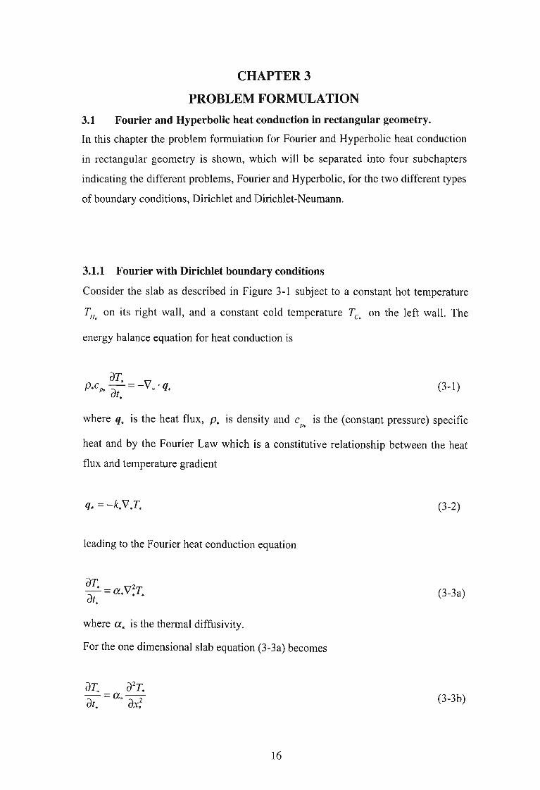
3.1.1 Fourier with Dirichlet boundary conditions
Consider the slab as described in Figure 3-1 subject to a constant hot temperature
TH• on its right wall , and a constant cold temperature Te• on the left wall. The
energy balance equation for heat conduction is
o,c aT. - -v .q* p* ":\ - * *ot,
where q. is the heat flux, P. is density and cp,
(3-1)
is the (constant pressure) specific
heat and by the Fourier Law which is a constitutive relationship between the heat
flux and temperature gradient
q. = -k.V.T.
leading to the Fourier heat conduction equation
aT. = a.V;T.at.
where a. is the thermal diffusivity.
For the one dimensional slab equation (3-3a) becomes
16
(3-2)
(3-3a)
(3-3b)

T==O
9ou
T
J
x*
J L
x* =0 x* =1L * L *
Figure 3-1: Problem formulation of heat conduction in a slab subject to constant
temperature (Dir ichlet) boundary conditions.
17

3.1.2 Fourier heat conduction with Dirichlet-Neumann boundary conditions
Consider the slab as described in Figure 3-2 subject to a constant heat flux on its
right wall qL*' representing the heat flux from the hot strip to the fluid due to the
uniform Joule heating generated in the thin hot strip by the electric current, and a
constant cold temperature Te• on the left wall. The Fourier conduction phenomenon
is governed by the constitutive relationship between the heat flux and temperature
gradient in the form shown in equation (3-2) and the energy balance equation (3-1),
which lead to the Fourier heat conduction equation (3-3a).
Tci 2R
qL**4nk*L *
9 b0U l:O
1 J
x*
L*
x* =0 x* =1L * L *
Figure 3-2: Problem formulation of heat conduction In a slab subject to a
combination of constant temperature (Dirichlet) and constant heat flux (Neumann)
boundary condition.
18

3.1.3 Hyperbolic heat conduction with Dirichlet boundary conditions
Consider the slab as described in Figure 3-1 subject to a constant temperature TH
• on
its right wall , and a constant cold temperature Tc on the left wall. The hyperbolic
conduction phenomenon is governed by the constitutive relationship between the
heat flux and temperature gradient in the form
aq. nr .-+q. =-k. vJ;at. (3-4)
where r , is the relaxation time and a. is the thermal diffusivity, which combined
with the energy balance equation (3-1) leads to the hyperbolic heat conduction
equation
_1 a2T. + _1 aT. =V2T
2 2 • •c. at. a. at. (3-5)
where c. =~a./r. is the speed of wave propagation. Equations (3-4) and (3-5) may
be transformed into a dimensionless form by introducing the following scales
L. , ti ]«. for the space variable and time variable, respectively. This leads to the
following definitions of the dimensionless variables
x.x = -
L. '
a. t,t = - 2- '
L.(3-6 )
that transform equations (3-4) and (3-5) into their corresponding dimensionless form
aqFo-+q=-VTat (3-7)
(3-8 )
where Fo = a.r.IL: is the Fourier number. For the one-dimensional slab considered
here equations (3-7) and (3-8) take the form
aq aTFo-+q=--at ax
19
(3-9)
(3-10)

The analysis and investigation of equation (3-10) was extensively covered in
excellent papers and reviews, such as Ozisik and Tzou (1994), Haji-Sheikh,
Minkowycz and Sparrow (2002), Wang (2000), Frankel, Vick and Ozisik (1985),
and Vick and Ozisik (1983), to name only a few. The boundary and initial conditions
are expressed in the following dimensionless form
x = O: T = O
x=I:T=1
{T = To = const.
t = 0: . .T =To =const.
(3-11)
(3-12)
3.1.4 Hyperbolic heat conduction with Dirichlet-Neumann boundary
conditions
Consider the slab as described in Figure 3-2 subject to a constant heat flux on its
right wall qL" representing the heat flux from the hot strip to the fluid due to the
uniform Joule heating generated in the thin hot strip by the electric current, and a
constant cold temperature Tc on the left wall. The hyperbolic conduction
phenomenon is governed by the constitutive relationship between the heat flux and
temperature gradient in the form shown in equation (3-4), leading to the hyperbolic
heat conduction equation (3-5) .
Equations (3-4) and (3-5) may be transferred into a dimensionless form by
introducing the following scales L., L:/a., IqL*l , IqL*IL./k. for the space variable,
time variable, heat flux and temperature difference, respectively. This leads to the
following definitions of the dimensionless variables
x.x =
L. 'a. t,
t=-2-'L.
(3-13)
that transform equations (3-4) and (3-5) into their corresponding dimensionless form
dqFo-+q=-'lT
dt
20
(3-14)
(3-15)

where Fo = a.t.]L: is the Fourier number. For the one-dimensional slab considered
here equations (3-14) and (3-15) take the form
aq aTFo-.t+ q =--at .r ax (3-16)
(3-17)
(3-18)
The analysis and investigation of equation (3-17) was extensively covered in
excellent papers and reviews, such as Ozisik and Tzou (1994), Haji-Sheikh,
Minkowycz and Sparrow (2002), Wang (2000), Frankel, Vick and Ozisik (1985),
and Vick and Ozisik (1983), to name only a few. The boundary and initial conditions
are expressed in the following dimensionless form
x=O: T=Ox= 1: qL = -1 ~ (aTlaxt:1 = 1
_ . {T = To= const .t - O. . .
T=To=const.(3-19)
Note that because the boundary heat flux atx = 1 is constant, equation (3-16) with
(aqjaft:1= 0 , produces (qJX: l= -(aTlaxt:I ' a result that is identical to the
Fourier boundary condition.
21

3.2 Fourier and Hyperbolic heat conduction in cylindrical geometry.
In this chapter the problem formulation for Fourier and Hyperbolic heat conduction
in cylindrical geometry is shown, which will be separated into two subchapters
indicating the different problems, Fourier and Hyperbolic , for the boundary
conditions Dirichlet-Neumann.
3.2.1 Fourier heat conduction with Dirichlet-Neumann boundary conditions
Consider the cylinder as described in Figure 3-3 subject to a constant heat flux at rw•
qL. ' representing the heat flux from the hot wire to the fluid due to the uniform Joule
heating generated in the thin hot wire by the electric current, and a constant cold
temperature Te• at ro.' The Fourier conduction phenomenon is governed by the
constitutive relationship between the heat flux and temperature gradient in the form
shown in equation (3-2) and the energy balance equation (3-1), which lead to the
Fourier heat conduction equation
a2T. 1 aT. 1 ot;--+--=---ar.2 r. ar. a. at. (3-20)
where r, is the independent variable in the radial direction and a. is the thermal
diffusivity.
Equation (3-20) may be transformed into a dimensionless form by introducing the
following definitions of dimensionless variables
r = ~ro'
(3-21)
that transform equation (3-20) into its corresponding dimensionless form
a2T 1 er er-+--=-ar 2 r ar at
22
(3-22)

The boundary and initial conditions are expressed in the following dimensionless
form
aTr=r . -=-1
w· arr=I:T=O
{T =To=const.
t =0: . .T = To= const.
(3-23)
(3-24)
3.2.2 Hyperbolic heat conduction with Dirichlet-Neumann boundary
conditions
Consider the cylinder as described in Figure 3-3 subject to a constant heat flux at rw
•
qo. ' representing the heat flux from the hot wire to the fluid due to the uniform Joule
heating generated in the thin hot wire by the electric current, and a constant cold
temperature Te• at roo . The hyperbolic conduction phenomenon is governed by the
constitutive relationship between the heat flux and temperature gradient in the form
shown in equation (3-4), leading to the hyperbolic heat conduction equation (3-5).
Equations (3-4) and (3-5) may be transferred into a dimensionless form by
introducing the following scales ro., ro~ / a., qo., qo.L. / k. for the space variable,
time variable, heat flux and temperature difference, respectively. This leads to the
following definitions of the dimensionless variables
a .t,t=-2-'
roo
q.q=-,
%.(3-25)
that transform equations (3-4) and (3-5) into their corresponding dimensionless form
aqFo-+q=-VTat (3-26)
(3-27)
where Fo =a.r./ro~ is the Fourier number. For the one-dimensional slab considered
here equation (3-27) takes the form
23

(3-28)
(3-29)
The boundary and initial conditions are expressed in the following dimensionless
form
r = r : aT =-1w ar
r=I:T=O
{T =To=const.
t =0: . .T =To=const.
(3-30)
Note that because the boundary heat flux at r = rw
is constant, equation (3-26) with
(aqjatt =r = 0, produces (qrt=r = - (aTjart=r ' a result that is identical to thew w w
Fourier boundary condition.
24
dW*
~%%'{ifJ.g;)iS2···············f}Uit!······ ····
~Ifllm
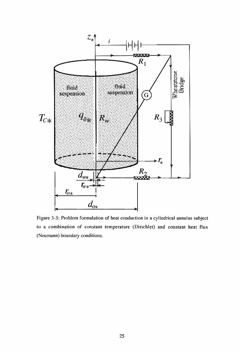
Figure 3-3 : Problem formulation of heat conduction in a cylindrical annulus subject
to a combination of constant temperature (Dirichlet) and constant heat flux
(Neumann) boundary conditions.
25
CHAPTER 4
SOLUTION TO HYPERBOLIC HEAT CONDUCTION
PROBLEM
4.1 Solution to the Heat Conduction Problem in rectangular geometry
In this chapter the solution for Fourier and Hyperbolic heat conduction in rectangular
geometry is shown, which will be separated into five subchapters, four indicating the
different problems, Fourier and Hyperbolic, for the two different types of boundary
conditions, Dirichlet and Dirichlet-Neumann, and one subchapter for the calculation
of the time needed by a pulse to cross the gap.
4.1.1 Solution to the Fourier heat conduction problem subject to Dirichlet
boundary conditions.
While the objective of this chapter is to present the derivations of the solutions to the
hyperbolic heat conduction problem the first step is to show the solution to the
corresponding Fourier heat conduction. The reason for the latter is the need to have
the reference Fourier solution for comparison purposes as will be shown later.
Equation (3-3b) has a steady state solution as follows
TH• - Te.Ts = x, + Te. L* .
Using the following definitions of dimensionless variables
(4-1)
x*x=-L* '
(4-2)
equation (4-1) can be transformed into its dimensionless form
T =xs (4-3)
The transient solution to equation (3-3) is obtained via separation of variables and
can be presented as follows
T - L~ C - a . (mn:l L, j 2 t• • (mnx*)-·e ·sm --t, m L
m= 1 *
where Cm is a constant which is derived from initial conditions in the form
26
(4-4)

(-1r(1- To) + ToC = C = 2..:.....--'---''-------'--
m n · nn
Using the following definitions of dimensionless variables
(4-5)
X.x =
L '.a. t,
t=--L2. (4-6)
equation (4-4) can be transformed into its dimensionless form
00
t, = LCn
· e-(nTd r ·sin(nx)n= 1
(4-7)
Equations (4-3) and (4-7) now show the temperature profile in space and time as
follows
00
T(t,x) =T, +T, =x + LCn
• e- (n1d r• sin(nx)
n= 1
4.1.2 Solution to the Fourier heat conduction problem subject to a
combination of Dirichlet and Neumann boundary conditions.
(4-8)
As in the previous section equation (3-3b) still applies but with the different
boundary conditions. The solutions to steady state, transient and final temperature
equations in a dimensionless form are obtained via separation of variables and can be
presented as follows
T =xs
00 - ( !E.+nrrrr [( n )]T, =~Cn • e 2 • sin "2 + nn x
T,( ~ -v mt)-(-1)"where C = 2 --'--------''----
" (~ + rat ) '
27
(4-9)
(4-10)
(4-10)
(4-11 )

4.1.3 Solution to the Hyperbolic heat conduction problem subject to Dirichlet
boundary conditions.
The solution to equation (3-10) subject to the boundary and initial conditions shown
by equations (3-11) and (3-12) is expressed in terms of orthogonal eigenfunctions
obtained via separation of variables in the form
Mo
T=x+eAc1'L[An/',n1+Bne~,"IJsin[nnx]+n=O .
(4-12)
~n [sin(nttx - A;i) + sin(nttx + Ain!)J}where
and where the following notation was introduced
(a)
(b)
(c)
(4-13)
1 ~ 2 2~ = - - 1- 4n n Fa ." 1In 2Fa '
1 ~ 2 2~JlI =- 1- 4n n Fa ;
2Fa
1 ~ 2 2~A= - 1-4n tt FaFa
1 ~ 2 2A;n= -- 4n n Fa -12Fa
(a)
(b)
(c)
(4-14)
while the critical value of n , i.e. n cr' was evaluated and can be expressed in the form
1n =--==
cr 2nJji; (4-15)
For initial conditions consistent with an initial permanent constant temperature
identical to that of the environment, i.e. to Te* , the dimensionless values of the initial
28

conditions are To= 0, t o= 0, leading to the following expressions for the
coefficients in the series (4-12)
2AAn =- II... c lIn; B; =21ln ;
In
(a)
(b)
(c)
(4-16)
where lIn = (-If [nn .
The infinite series in equation (4-12) consists of three separate contributions dictated
by the values of M ; and M I defined by
V ncr = j, j =0,1,2,3, .
V ncr ::t. j, j = 0,1,2,3, ..
V ncr = j, j = 0,1,2,3, ..
Vncr::t.j, j=0,1,2,3, ..
(4-17)
(4-18)
where 8 . is the Kronecker delta function defined in the formncr '}
{
I8 . =
ncr,J 0V ncr = j, j =0,1,2,3, ..
Vncr::t.j, j=0,1,2,3, ..(4-19)
and Ln.;Jis the inclusive floor function representing the largest integer less than or
equal to ncr ' Therefore M 0 is the exclusive floor function representing the largest
integer less than ncr' The first contribution is a finite series for the terms
corresponding to values of 0 < n < ncr' When ncr =0 corresponding to Fo=l/rc2
this contribution is absent. The second contribution is the critical term which is
present only if ncr is a non-negative integer. This critical term is absent when ncr is
not a non-negative integer, or if Fo> l/rc2• The third contribution is an infinite
series representing traveling waves that formed via a cascade of frequencies over a
wide range of scales. This contribution is present at all times however it may become
significantly small if ncr » 1.
The primary interest is the temperature value at x = 1, or dimensionally at x, =L. ,
i.e. TL • The latter is obtained by substituting x = 1 into the solution (4-12) leading to
29

[
MO
TL = 1+ eAcl ~(aneA" nl + bne~,n') + (an.cr + bn.crt) 8n" .j
+"~, [a" sin (A,"1) +b"cos (Aj)]] •
where the coefficients are defined as follows
(4-20)
( )n 2~n
an = -1 An = ntmA- ;
-2A-b =(_I)n B =__In .n n nn~A-'
2an•cr =(-Ira An•cr= - ;
nn_ (l)na _ -2 A-c .bn.cr - - Bn.cr - -- ,
nn
-2A-a =(_I)nA =_c .n n.'l '
nn/\'in
b =(_I)n B =~.n n 'nn
(a)
(b)
(c)
(4-21)
Therefore the temperature TL (t) at x =1, or dimensionally at x, =L. , can be
presented following equation (4-20) in the following form
()[ Tu (t )- Te•] k. ( )
TL t = I I = 1+h tqL' L.
where
h (t) = eAcl[~(a eA" nl + b e~,"I) + (a + b t) 8 ..£..J n n n,cr n. cr ncr,Jn=O
+"~, [a"sin (A,"I) +b" costA",I)] ]
which produces the following dimensional solution
30
(4-22)
(4-23)
(4-24)

4.1.4 The time needed for a pulse to cross the gap in rectangular geometry.
From equation (3-5)
(4-25)
where c. is the speed of wave propagation. Any signal (pulse) will propagate in the
x, direction with speed c• . It will cross the gap traveling a distance L. = c.t L' ,
where t L' is the time needed for the wave to cross the gap, and therefore
(4-26)
From equation (3-8) the dimensi~nless speed of wave propagation is ~ and the"Fo
dimensionless gap length is I. Therefore, the dimensionless time needed for a pulse
to cross the gap is
ItL =-I-=.jF;
.jF;
31
(4-27)
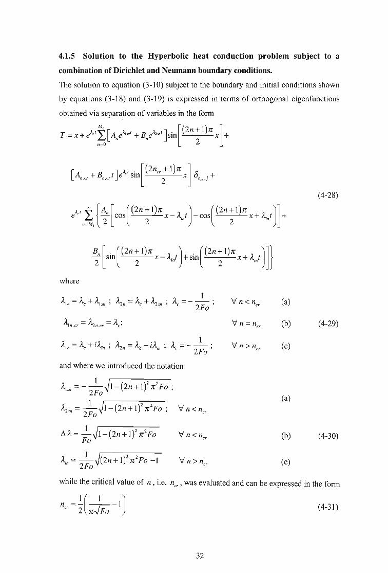
4.1.5 Solution to the Hyperbolic heat conduction problem subject to a
combination of Dirichlet and Neumann boundary conditions.
The solution to equation (3-10) subject to the boundary and initi al conditions shown
by equations (3- 18) and (3-19) is expressed in terms of orthogonal eigenfunctions
obtained via separation of variables in the form
A t ~ [ A t 1 tJ . [(2n+l)Jr ]T = x + e C £..J Ane Isn + Bne "1. sn sm x +n=O 2
(4-28)
A t ~ {A [ ( (2n + 1)Jr J ((2n + 1)Jr J]e C n~1 ---:t cos 2 x - Aint - cos 2 x + Aii +
e, [ . ( (2n + l )Jr 1 J . ( (2n + l )Jr 1 J]}- sm x-/\,. t +sm x +/\,. t2 2 In 2 In
where
and where we introduced the notation
A,sn=- _1_~1_ (2n + 1)2Jr2Fo ;2Fo
\ sn= _1_~I-(2n+l)2Jr2Fo ; V n<»;2Fo
~A= _1~1-(2n+l)2Jr2FoFo
Vn=ncr
(a)
(b)
(c)
(a)
(b)
(4-29)
(4-30)
(c)
while the critical value of n , i.e. ncr ' was evaluated and can be expressed in the form
ncr =!( ~-1)2 n Fo
32
(4-31)
For initial conditions consistent with an initial permanent constant temperature
identical to that of the environment, i.e. to Te. , the dimensionless values of the initial
conditions are To=0, t o=0 , leading to the following expressions for the
coefficients in the series (4-28)
A = _2_~=n,--,ll:.:.:..nn LU.
(a)
2,1,An = - A.. c lin ; B, = 21ln ;
In
"i/n=ncr(b)
(c)
(4-32)
The infinite series in equation (4-28) consists of three separate contributions dictated
by the values of M; and M( defined by
V ncr = j ,
V ncr * j ,
V ncr = j ,
"i/ ncr * j ,
j = 0,1,2, 3, .
j = 0,1,2,3, .
j = 0,1,2,3, .
j = 0,1,2 ,3, .
(4-33)
(4-34)
where 0 . is the Kronecker delta function defined in the formneT'}
"i/ ncr = j ,
"i/ ncr * j ,
j = 0,1,2,3, .
j = 0,1,2, 3, .(4-35)
and Lncr Jis the inclusive floor function representing the largest integer less than or
equal to ncr' Therefore M 0 is the exclusive floor function representing the largest
integer less than ncr' The first contribution is a finite series for the terms
corresponding to values of °< n < ncr' When ncr =°corresponding to Fo =1/n 2
(see equation 4-31) this contribution is absent. The second contribution is the critical
term which is present only if ncr is a non-negative integer. This critical term is
absent when ncr is not a non-negative integer, or if Fo> l/n2• The third
contribution is an infinite series representing traveling waves that formed via a
cascade of frequencies over a wide range of scales. This contribution is present at all
times however it may become significantly small if ncr » 1.
The primary interest is the temperature value at x = I, or dimensionally at x, = L. ,
i.e. TL • The latter is obtained by substituting x = 1 into the solution (4-28) leading to
33

[
MO
T = l+ / cl ~(a eA" nl +b e~,"I ) + (a +b t) 8 .L £..J n n n,cr n,cr nCT ' }
n=O
+ "~, [a"sin(Ai"f) +b; cos( A,"f)J]
where the coefficients are defined as follows
a - (_l)nA _ - 8 ~n .n - n - (2n + 1)2n2~A '
b - (_l)nB _ 8A,n . \-I <n - n - (2n + 1)2 n 2~A ' v n ncr
-8an•cr = (-1t r
An•cr= (2n + 1)2n2 ;
b =(_ l )ncr B = 8 Ac2 2; V n =n cr
n.cr n.cr (2n + 1) n
a = (_l)nA = 8 Ac
n n (2 1)2 21.n + n A.m
n - 8b, =(-1) B; = (2n +1)2
n2 ; Vn>ncr
(a)
(b)
(c)
(4-36)
(4-37)
Therefore the temperature TL (t) at x = 1, or dimensionally at x, = L. , can be
presented following equation (4-36) in the following form
( )_ [TL.(t)-Tc.Jk. _ ( )TL t - I I - 1+ h t
qL' L.
where
h(t)= eAcl[~(a eA"nl + b e~,nl) + (a + b t) 8 .£..J n n n.cr n.cr ncr. jn=O
+"~, [a"sin(Ai"f) + b" cos(Ai"f)]]
which produces the following dimensional solution
34
(4-38)
(4-39 )
(4-40)

4.2 Solution to the Heat Conduction Problem in cylindrical geometry
In this chapter the solution for Fourier and Hyperbolic heat conduction in rectangular
geometry is shown, which will be separated into three subchapters, two indicating
the different problems, Fourier and Hyperbolic , for the boundary conditions
Dirichlet-Neumann, and the last subchapter for the calculation of the time needed by
a pulse to cross the gap.
4.2.1 Solution to the Fourier heat conduction problem subject to a
combination of Dirichlet and Neumann boundary conditions.
While the objective of this chapter is to present the derivations of the solutions to the
hyperbolic heat conduction problem the first step is to show the solution to the
corresponding Fourier heat conduction. The reason for the latter is the need to have
the reference Fourier solution for comparison purposes as will be shown later.
Equation (3-22) has a steady state dimensionless solution as follows
T =-r lnrs w
and a transient solution obtained via separation of variables in the form
T =~ a e- f3;'R, ~ n On
n=O
where an is represented by the following equation
I ( - 12a =-:....._=-
n I3
and / 1,12,13 are definite integrals with the following solutions
(4-41)
(4-42)
(4-43)
TO [ 2 ()]I=----rR rI f3
nnf3
nW 0 f3n , W
35
(a)
(b)
(c)
(4-44)
where R is represented by a linear combination of Bessel functions as follow sOn
(4-45)
and f3n's are the positive roots of the follo wing
(4-46)
where 10 and Yo are the order 0 Bessel functions of the fir st and second kind ,
respecti vely.
This leads to the final solution for the temperature as follows
T=T +T =-r Inr+~ a e- f3;tRo (f3 ,r )s I w £..J n n n
n=O
(4-47)
4.2.2 Solution to the Hyperbolic heat conduction problem subject to a
combination of Dirichlet and Neumann boundary conditions.
The solution to equation (3-28) subject to the boundary and initial conditions
obtained via separation of variables by equations (3-29) and (3-30 ) is expressed in
terms of orthogonal eigenfunctions in the form
n cr -1
T = r,+ T, = r r; Inr + L AnI (/ II/FO- ANDleA,.t/FO)Ro(f3nr) +n=1
(4-48)ee
L Ana/,t /Fo[COS (Aii / Fo)- AND2 sin (A;nt / Fo)JRo(f3nr)ncr +1
where
~.2 = - ~(1±~l- 4Fof32) V f3 < f3cr (4-49)
1A=-- V f3 = f3cr (4-50)
2
IA =-- V f3 > f3cr (4-5 1)r 2
A. = !~4Fof32 -1 V f3 > f3cr (4-52)In 2
36

(a)
(b)
(c)
(4-53)
(4-54)
(4-55)
and 11,1
2,1
3are definite integrals with the following solutions
(a)
(b)
(c)
(4-56)
where Ron is represented by a linear combination of Bessel functions as follows
(4-57)
and f3n's are the positive roots of the following equation
(4-58)
where Jo and Y o are the order 0 Bessel functions of the first and second kind,
respectively.
The critical value of n , i.e. ncr ' cannot be evaluated analytically but only
numerically. f3er can be expressed by equating the square root in equation (4-49) to
zero, as follows
1f3er = 2.Jji;
37
(4-59)
4.2.3 The time needed for a pulse to cross the gap in cylindrical geometry.
The dimensionless distance between the wire and the cylinder wall is (1- rw ) and the
dimensionless speed of wave propagation from equation (3-8) is 1/.JFa, hence the
dimensionless time needed for the thermal pulse to cross the annulus gap is
Its corresponding dimensional time is
t =(ro- r )~1:./a.w. • w.
38
(4-60)
(4-61)

CHAPTERS
RESULTS AND DISCUSSION
5.1 Analytical solution evaluated using Fortran.
All the results of temperature as a function of time and space presented in the
previous section were evaluated by Fortran programming. Also the results for the
thermal conductivity ratio and wire temperature versus time were derived using
Fortran programming. The Fortran computer language programs were written to
show results of temperature vs. time and vs. space for Fourier and Hyperbolic heat
conduction in rectangular and cylindrical geometries. In the rectangular geometry the
space is represented by x and in the cylindrical one by r, where x and r represent the
independent variables in each coordinate system respectively. The results were then
plotted graphically to observe the outcome. The numerical method used to calculate
~ is ZBRENT, which is found in the numerical recipes in the Fortran program.
ZBRENT is the combination of advantages of the bisection and Ridders methods of
root finding . The accuracy of the root is 10-7 •
39

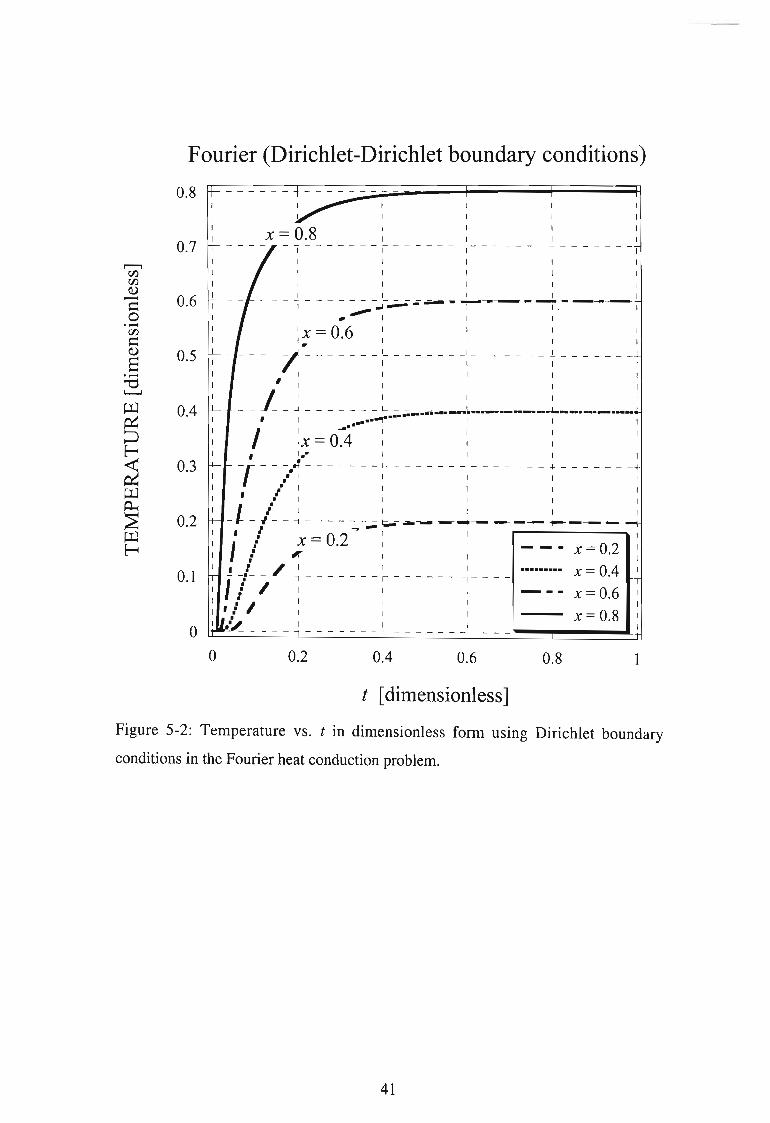
5.2 Results for the Fourier heat conduction problem subject to Dirichlet
boundary conditions.
The computed analytical results of temperature vs. x and vs. t for Fourier heat
conduction subject to Dirichlet boundary conditions at different t and x values,
respectively are being presented in Figures 5-1 and 5-2. As expected the temperature
profile moves from right to left with increasing time until steady state is reached at t
=0.5 as shown in Figure 5-1. Figure 5-2 shows the expected temperature profile vs.
time at different points in the medium. The results correspond to those in Figure 5-1
which shows that steady state is reached at t =0.5 as the temperature curves level to
a constant line parallel to the time axis.
Fourier (Dirichlet-Dirichlet boundary conditions)
fr t 20.001 : -~ t - - - ~-j: : : ,,~~I ••••••••• t = 0.01 I I , .I' i I
I I I I , ""/:1
0.8 ~ - - t = 0.05 - - :- - - - - - - _: - - - - - - - J.,:-! -j :, I "/: II I • •
I _ ••• - t = 0.1 " I I ! :I , I I : I
I , I "" / : II ----- t = 0.5 I ' I :I I I ' I : II
, I :
0.6 :-' - - - - - -: - - - - - - - : - - - -, = O~5 . - - -; "'- ~ / - - -r-L:I I I ' "/: i II I I I' .. I : I
I I I , I / I i I
I I I ' I I ' : I
I I I ' I " " / ' : I0.4 ~ - - - - - - ~ - - - - - -,-( - - - - - - -1 --- --: --f -- -~
I I , I • I " I t = O.05! I
I I ' I / I , : II I ' I I : II I , ' I .. 1/ ! II I , I · I I : I
I I ' 1 / I 1/ I0.2 ,- - - - - - - ~ - - - - - - - 1,,0- - - - - - - I - - - - - - - T:- - - - - - T
I " I /' / I ,. I
I " •• I I ."J I II , I ",. I / 1
I , I . . I / I I t = 0.001I , ."". ~ 0". I JI' ' ~.. I ~ ••,.~ __ I . _ Io 1-.. --- I L •••••• 1
0.4o 0.2 0.6
x [dimensionless]
0.8
Figure 5-1: Temperature vs. x in dimensionless form using Dirichlet boundary
conditions in the Fourier heat conduction problem.
40
Fourier (Dirichlet-Dirichlet boundary conditions)
x= 0.8
I II I
I I
I I- 1 - -- - - - - , - - - - - - -- - - - - -- 1 - - - - - - -
I I I
I I I
I I I
I I I I- - - - - - - - - - -_-..-.- - --- .. ------1.------ --- I I
:x = 0.6 : I : I___ _ _ _j .r L I J I
, ~ I I I II I I I I
, I I I I I
__ J _~ ~.;;. -~~~~.----~--.--.-- I, I ••••••.., I I I
II ~
IX = 0.4 I I I I
, I.- I I I I--r--/.~-------~ -------:-------~ -------I
• I I I I I, l I I I I I
-1-i--~ -------~ ~ ~__- I. ~-
"
i X = 0.2 : : - - - x = 0.2:;r I I•.! _1_- / - ~ - - - - - - - ~ - - - - - - -:- - - - •••..•... x = 0.4, ; I I I I - - - x = 0.6
• I I I
'l I I I I X = 0.8.~ - - - - I I I _
0.1
o
0.3
0.4
0.5
0.2
0.6
0.7
0.8
o 0.2 0.4 0.6 0.8
t [dimensionless]
Figure 5-2: Temperature vs. t in dimensionless form using Dirichlet boundary
conditions in the Fourier heat conduction problem.
41
5.3 Results for the Fourier heat conduction problem subject to a
combination of Dirichlet and Neumann boundary conditions.
5.3.1 Rectangular geometry.
With the combination of Dirichlet and Neumann boundary conditions Figure 5-3
shows how the temperature reaches steady state as the temperature profile develops
moving from right to the left. The difference between this case and that of Dirichlet
Dirichlet boundary conditions is seen at the right wall (boundary). While in Figure 5
1 the temperature at the right boundary is always constant at 1, Figure 5-3 shows
how the temperature starts just below 0.2 for a time t = 0.02 and rises to 1 at t = 5.
This is the case since there is a constant heat flux applied to this boundary shown in
Figure 5-3 by the constant slope of the curves at x = 1 and a constant temperature in
Figure 5-1. The constant heat flux would cause a constant temperature gradient at the
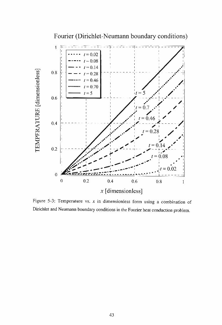
boundary, which is seen in Figure 5-3. In Figure 5-4 the temperature is plotted versus
time at different values for x.
42
Fourier (Dirichlet-Neumann boundary conditions)
..... t= 0.02---_. t = 0.08--- t = 0.14
0.8 - -- t = 0.28_ .... t = 0.46......... t = 0.70
t = 5
1
0.6
0.4
0.2
o
I
IIIIII
_ _ _ _ _ _ ...1 _
I
I
I
I
I
I
~.•.
I, I
I / . :
~' .' I
t = 0.08 . 1• I
I • II • I
I t = 0.02 II
o 0.2 0.4 0.6 0.8
x [dimensionless]
Figure 5-3: Temperature vs. x in dimensionless form using a combination of
Dirichlet and Neumann boundary conditions in the Fourier heat conduction problem.
43
Fourier (Dirichlet-Neumann boundary conditions)
5
x = 0.2
x=O.4
x=0.6
x = 0.8
x = l
4
----------
32
1 II I
I I
I I
I I I
x= 1 I I I- - - - - T - - -....;.~••.-X = 0.8 - "i---_..r---~-
I •• - I I
.~ I I•• I I I
I I : :
- -l-- - 1- - - - - .-- IX = 0.6 - I
I 1 .. -- I I
/f I I.. , I I I
'
" I 1 1 II I I
_ 1 - 1 - - _.L - - - - - ..."..I,x - 0 4 ._... .L ._: 1 .···········1 - · I III ....·r· I I I
I •• I I I I",. I I I 1
il1·( - - _l _- - - --_IX = 0 2 _l- .: _: • • ... -- - - • I .------:....1 ----,.
1/: ", I I I _
: I I II I / I I I..il I I I
I I I- - - - - - T - - - - - - - 1- - - - - - - - I - - - ---- - -
I I I
I I I
I I I
I I I
I I I
o
o
0.4
0.2
0.6
0.8
-0.2
t [dimensionless]
Figure 5-4: Temperature vs. t in dimensionless form using a combination of Dirichlet
and Neumann boundary conditions in the Fourier heat conduction problem.
44

5.3.2 Cylindrical geometry.
The results of temperature vs. r at different values of time are presented in Figure 5-5
for Fourier heat conduction in a cylindrical geometry. Here the steady state is not as
easy to recognize because it is logarithmic rather than linear in r, which leads to
Figure 5-6 , which shows the r axis on a logarithmic scale . This way it is easier to
recognize the steady state since a straight line as seen in Figure 5-6 represents it. In
Figure 5-7 the temperature is plotted versus time, but now with different values for r,
one of which is the inner radius (r w = 0.002). Since there is a heat flux at this
boundary the temperature is not constant as can be seen until steady state is reached.
Fourier (Dirichlet-Neumann boundary conditions)
0.014
0.012
0.01
0.008
0.006
0.004
0.002
oo 0.2 0.4 0.6
r [dimensionless]
0.8
t = 0.01
t = 0.05
t = 0.15
t = 1.5
Figure 5-5:Temperature vs. r in dimensionless form using a combination of Dirichlet
and Neumann boundary conditions in the Fourier heat conduction problem.
45

Fourier (Dirichlet-Neumann boundary conditions)
0.014
o0.001
t = 0.15
t = 0.05
t = 0.01
t = 1.5
0.10.01
1
1
1
I 1- - - - - - - 1- - - - - - - - - - - - T"
I 1
1 I
• 1 I
~ '. 1 1- - - .- - , - - - 1- - - - - - - - - - - - 1-
, • 1 I '------..• • I
, " 1 1, • 1 I, , .
_ _ __~ - - -L --~ - - L _
" 'I, I, • 1 1
" ~. -. I"" I", 1
" 1 • I- - ---- - -- , - -- ~- - ,- - - - - - -- - - -- -- - - -,I • _ I
I, '-, I1 " II " , .I ' ','. I
- - - - - - - - - - -1 - - - ~, - - - r - ~ r -1 , , .~
1 ",', I',1 " 1
1 ,,"'." . .- - - - - - - - - - - 1- - - - , _ _ L ~; _ ~ _
1 , I , •I , I .-.
I ~, '.'I I', '. -..I I ..... _ 1IIliIIIII_ ... '_.
- --- - -- - -- - - - - --- -- - - - - -- - - ~ - __r_~
0.01
0.006
0.002
0.004
0.012
0.008
log(r) [dimensionless]
Figure 5-6:Temperature vs, log(r) in dimensionless form using a combination of
Dirichlet and Neumann boundary conditions in the Fourier heat conduction problem.
46

Fourier (Dirichlet-Neumann boundary conditions)
--
r = 0.002
r = 0.25
r = 0.5
r = 0.75
I I I I I1 I 1 1 11 1 1 1 11 I I I 1
1 1 J __ - - - - - - - I r = 0.002 ' I - - - - - - - - -rr - - - - - - I - ;; .-.- .. ~ -- r - - - - - - -, 1- - - - - - - -1 _ ~ - 1 1
I • •• I I I
1 - I I II · 1 1 1~ _ ~ ~ L J _-
1 I 1 1 11 I 1 1 I1 • I 1 1
II. 1 1 1I. I I I~ - - --- -~ - - ---- -r ---- - - l - - I
f 1 1 I 1
t i l 1 1
• 1 1 1 1, I I 1 1
~ - - - - - - -I - - - - - - - ~ - - - - - - ~ - - - - - - - 1- - - - - - --
I 1 1 1 II 1 I I 1
• 1 1 1 1I 1 1 1 IH- - - - - - - _I _ - - - - - - 1- ...! 1 _
I 1 1 1 1I 1 1 1 1, 1 1 1 I
! 1 I _-------.,.r = 0 25 -,---------· ..... .• 1. - -- -- I I I-. - - - - - ,.-r'- - - - - - - r - - - - - - .., - - - - - - - 1- - - - - - --
I ,- I I 1 1!,. I 1- - - - - Ir= 0.5 -"1- ---I· ...",,-- 1 1 ,
I I' ". - ..J _ - - - .,.. - - - - ,r = 0.75 . .,. - - - -o~~~- '::1 - - - - - - - f-- - - - - - - --l - - - - - - -1- - - - - - - -
0.01
0.002
0.004
0.006
0.008
0.012
0.014
o 0.2 0.4 0.6 0.8
t [dimensionless]
Figure 5-7:Temperature vs. t in dimensionless form using a combination of Dirichlet
and Neumann boundary conditions in the Fourier heat conduction problem.
47

5.4 Results for the hyperbolic heat conduction problem subject to Dirichlet
boundary conditions in rectangular geometry.
In hyperbolic heat conduction the Fourier number plays a significant role as it
impacts the temperature in space and time. In Figure 5-8 one can see the evolution of
the temperature profile towards the steady state for F0 = 10-4• It is obvious that for
such a small Fourier number the hyperbolic conduction solution is expected to be
almost identical to the Fourier conduction solution presented in Figure 5-1. Indeed,
Figure 5-8 shows a nearly Fourier conduction result in terms of the evolution of the
temperature profile towards steady state. This anticipation is based on the fact that
equation (3-17 ) transforms into the Fourier diffusion equation when F 0 -7 0 (or
Fo-e: 1). No wave effects are visible in the results presented in Figure 5-8. Increasing
the Fourier number to Fo =0.01 as seen in Figure 5-9 causes discontinuity in the
temperature gradient that represents the location of the moving front transferring the
boundary temperature "signal" within the domain. This can be seen in Figures 5-10
to 5-12 for F0 =0.1. In Figure 5-10 the front moves from the right boundary to the
left with the moving front decreasing in magnitude. Figure 5-11 shows the front
moving back to the right boundary from the left (reflected back), while the moving
front magnitude decreases further. Finally Figure 5-12 shows the front moving
toward the left boundary again with steady state being achieved before the front
reaches the left boundary. The time needed for a pulse to cross the gap is calculated
using equation (4-27). It is seen that the temperatures reach steady state values for all
the x values . The graphs in Figures 5-13 to 5-15 show the temperature versus time at
different values for x for Fo =0.1. In all three Figures 5-13 to 5-15 it is seen that the
temperature reaches the expected steady state values. The discontinuity in Figures 5
13 to 5-15 before steady state is reached is due to the front propagation mentioned
earlier. At each point of discontinuity in Figures 5-13 to 5-15 the wave passes
through the corresponding value of x as it bounces back and fourth between the
boundaries. Figures 5-16 to 5-22 corresponding to F0 =1 show the front even better
as it moves from one boundary to the other and back over and over, until steady state
is reached at about t =9 (Figure 5-22). The moving front in Figures 5-16 to 5-22 is
also seen better as its amplitude reduces with time. In Figures 5-23 and 5-24 the
temperature is plotted versus time at different values for x and for F0 =10-4 and F0 =10-3, respectively. In Figures 5-23 and 5-24 there is no discontinuity as seen in
48

Figures 5-13 to 5-15 in the temperature. The reason for the lack of discontinuity in
temperature in Figures 5-23 and 5-24 is because the solution for such small Fourier
number follows almost identically the Fourier conduction solution. As mentioned
before, with a small Fourier number the hyperbolic conduction solution is almost the
same as for the Fourier conduction.
Figures 5-25 to 5-27 show the front propagation from boundary to boundary most
clearly. With Fa = 1 Figures 5-25 to 5-27 show the temperature versus time at
different values for x. The oscillatory effect is shown and explains the moving front
that starts and decays with time until steady state is reached. The time between peaks
shows the bouncing period of the pulse. The period is calculated using equation (4-
27) that is t =.JFa and is identical to the bouncing period revealed in the graphsp
plotted in Figures 5-25 to 5-27. To compare the values from equation (4-27) and the
graphs plotted for the time needed for a pulse to cross the gap, Figures 5-25 to 5-27
show the clearest comparison. One adjustment needs to be made to equation (4-27)
to account for this calculation in each of the Figures 5-25 to 5-27. Equation (4-27)
calculates the time for the pulse to cross the whole gap, whereas in Figures 5-25 to 5
27 the pulse is relative to different values of x. Looking at the graphs in Figures 5-25
to 5-27 the time between the beginning of each peak represent the time for the pulse
to cross the gap twice. Therefore from the graphs in Figures 5-25 to 5-27 for Fa = 1
the time between each peak is equal to 2. From equation (4-27) with Fa = 1 the time
needed for the pulse to cross the gap once is 1. Therefore the graphs in Figures 5-25
to 5-27 yield the expected results from equation (4-27). These results are seen for all
values of Fourier number. Looking at the graphs in Figures 5-13 to 5-15 with Fa =
0.1 the time between peaks is approximately 0.63. Substituting Fa = 0.1 into
equation (4-27) yields 0.316, which is approximately half of 0.63. This shows that
for all values of Fa the expected result from equation (4-27) is obtained from the
presented results.
49
-4Fa = 10
Hyperbolic (Dirichlet-Dirichlet boundary conditions)
0.6 0.8
x [dimensionless]0.40.2
t = 0.26
t = 0.08
t = 0.04I I
I , I
I ~~ II I II ' I
t = 0.12 ; : - - - - ~ ~~ - :
I I ~' I II I I /: II I : I
1 : : ~ / i '_,l____:I I I I , I ,
: : : I / / :iI 1 I I , .'I I I 1// "I I I I I I1 - - - - - - - : - - - - - t ='0.26 - -/-- ~/- ,. - - i-~ ------I I I ,' I
I I I I' I
I I 1 / ' I " II I I / 1 ," II I I I ' I
A' .1 - - - - - - _ 1- - - - 7" ;- 7 - - - -t = 0.04 - - ~ - - - - - -I /' I, ,.r I
I / 1 " I 1I .. I .' I I,I I •••- I II _..... I I
oo
0.4
0.2
0.6
0.8
Figure 5-8:Temperature vs. x in dimensionless form using Dirichlet boundary
conditions in the Hyperbolic heat conduction problem with Fourier number equal to
10-4 •
50

Fo = 0.01
Hyperbolic (Dirichlet-Dirichlet boundary conditions)
t = 0.1
t = 0.050
t = 0.0251
I
1
1 _I....1 I : /Ill
t = 0.075 - - : - - - - - - - :- - - - - - - : -;1,/1 1 1 : "1 1 1:1 ,I 1 IIi
1 1 1 • I ,_ _ _ _ _ _ J. --J 1 ._~ l
1 I I / I ii1 I I . ,
1 1 1 :/ ,'1I 1 I / ,. 1
1 1 I . , ' 1
------~ ------~ -------~~I /~ -:. ,I I .y' 1. ,1 1 / 1 , 11 1 I 1
1 I .· I " I
- ---- -~ - - - - - - ~ -~:_~-~~- -- -~ -- - - - -I J••/.'I 1
1 / 1 .' 11 ••• 1 •• I t = 0.0251 ./ /' r 1
,1-.. · 1••• 1 ~t = 0.075: 1........ ~ .
o
0.2
0.4
0.6
0.8
o 0.2 0.4 0.6 0.8
x [dimensionless]
Figure 5-9:Temperature YS. x in dimensionless form using Dirichlet boundary
conditions in the Hyperbolic heat conduction problem with Fourier number equal to
0.01.
51

Fo = 0.1
Hyperbolic (Dirichlet-Dirichlet boundary conditions)
I iI I
II I
II I
III
II I
I I
t> 0.12
t> 0.06
(=0.18
t> 0.24
t> 0.30
(= 0.32
- -- - - - - - --- -I
II
I I I I
I I I " I. ,I I ~. , I_ _ ~ - - - - - - ~ - - - - _ - ! L _
I I ~ 'I I~,. ,
I I 1:,•• I I I
I I ",,'l I I I
I I ~';,/ I: I
1 r.·// I I I
I ""~ I I I--~ ---~~~- ----:1 ------I
I "/ I I I I
I I .tI:.-/ I d II .... / I I I I
I ~'I/ I I: 1------~ -:IIf~/.~ -(- ----~ ------:i------I
I ,. I I I I
,,:'.. I I I II~'I(' I I d
- II ~ - I ' I I I II ,~" I : I I , I
" I I (=0.121 r-~ ----~ -:- --- /= 0.18 - - -: - - - - -1 I I I . , I I
I I I I I I
I (= 0.30 : 1
1I • I 1I I II • Io
0.2
0.4
0.6
0.8
o 0.2 0.4 0.6 0.8
x [dimensionless]
Figure 5-10:Temperature vs. x in dimensionless form using Dirichlet boundary
conditions in the Hyperbolic heat conduction problem with Fourier number equal to
0.1.
52

Fa = 0.1
Hyperbolic (Dirichlet-Dirichlet boundary conditions)
0.8
0.6
0.4
0.2
oo
t > 0.38t> 0.50
- ( =0.63
0.2 0.4
I
I
II
I_ _ __ _ _ -1 _
I
I
II
0.6 0.8
X [dimensionless]
Figure 5-11 :Temperature vs. x in dimensionless form using Dirichlet boundary
conditions in the Hyperbolic heat conduction problem with Fourier number equal to
0.1.
53

Fa = 0.1
Hyperbolic (Dirichlet-Dirichlet boundary conditions)
0.8
0.6
0.4
0.2
o
", ' I .'I "1 t= 0.63 ,,"
:I-m--- t ~ 0.95 , ••••I I I I ,,"
_ _ _ _ _ _ _ I _ _ _ _ _ _ _ .L _ _ _ _ _ _ _I _ _ _ _ _ _ _ '
I 1 I ,.'-1 I 1 II I 1
1 1 I1 1 II I 1
- - - - - - _1 - _ _ _ _ _ _ 1 ~ _
I 1I I
1 I
1 1
1 11 I
I 1- - - - - - -, - - - - - - - - - - - - - - - - - - - - - 1- - - - - - -
1 I
1 11 II 1
I I
1 1 1 I- - - - - - - r - - - - - - - I - - - - - - - r - - - - - -
1 I I I
1 I 1 I
I 1 I 11 I 1 I
1 1 1 1
I 1 I I
o 0.2 0.4 0.6 0.8
x [dimensionless]
Figure 5-1 2:Temperature vs. x in dimensionless form using Dirichlet boundary
cond itions in the Hyperbolic heat conduction problem with Fourier number equal to
0.1.
54
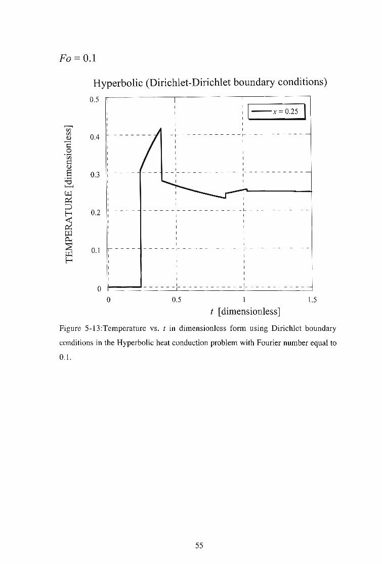
Fa = 0.1
Hyperbolic (Dirichlet-Dirichlet boundary conditions)
0.5
1.5
: I-X=0.25 I
1
t [dimensionless]0.5
1
1
1 1- - - - - - 1- - - 1 _
1 1
1 1
1 I
1 I
1 I
1 1- - - - - - 1- - - - - - - - - - - - 1- - - - - - - - - - -
1 1
I 11 1
1 1
I 1
1 1-- --- --- --- --- -- --- -- - - - -- ---
1
1
1
1
1 1
- - ~ - --- - - - -- - - ~ -- - - -- - - - -
1 1
1 11 11 11 1
- - - - - - - - _ 1- 1 _
1 11 1
1
oo
0.2
0.3
0.4
0.1
Figure 5-13 :Temperature vs. t in dimensionless form using Dirichlet boundary
conditions in the Hyperbolic heat conduction problem with Fourier number equal to
0.1.
55

Fo = 0.1
1.51
t [dimensionless]
: l-x=0.5 I1 1
1- - - - - - - - - - - - 1- - - - - - - - - - -1 11 1
I I1
0.5
- - - - - - 1- -
1
1
I
1- - - - - - - - 1- - - - - - - - - - - - - - - - - - - - - - -
1
I
1
1- - - - - - - - - -- -- -- - - - - - -- - - - - - - - - -I
1
1
1
- - - - - - - _1- _
1
1
I
1 1
- - - - - - - - 1- - - - - - - - - - - -1 - - - - - - _ - _ _ -1 1
I I
I I
1 1
o
0.1
o
0.2
0.3
0.4
0.5
0.6
Hyperbolic (Dirichlet-Dirichlet boundary conditions)
0.7
Figure 5-14:Temperature vs. t in dimensionless form using Dirichlet boundary
conditions in the Hyperbolic heat conduction problem with Fourier number equal to
0.1.
56
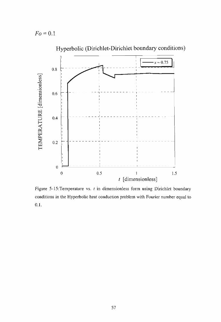
Fa = 0.1
Hyperbolic (Dirichlet-Dirichlet boundary conditions)
1.51
t [dimensionless]0.5
: : !-X=0 .75 I__ __ _ _ _ _ _ _ _ -1_
I I
I
I
III
I I- - ---- - - -,- --- ----- - - ,----- - - - ---
I I
I II II I
I II I
_ _ ___ _ ___ J l _I II I
I II I
I I
I I
I I
-- - - - - - - - ~ - - - - - - - ---- ~--- ------ - -
I I
I II I
I II I
I I
I I
oo
0.2
0.4
0.6
0.8
Figure 5-15 :Temperature vs . t in dimensionless form using Dirichlet boundary
conditions in the Hyperbolic heat conduction problem with Fourier number equal to
0.1.
57

Fa = 1
Hyperbolic (Dirichlet-Dirichlet boundary conditions)
0.6 0.8
x [dimensionless]0.40.2
t = 1
t = 0.6
t= 0.3II
I
I
I -ioI~ I
I- r---- r -- T - - - - - -
I I II
I I II
I I II
I I I
I II I 1 I
I II I : I- - - - - - 1- - - - - - - ~ - - - - - - r - - - 1- - - T - - - - - -
I I II I 1 I
I I I : II I I 1 I
II ~ I I 1 I''-.. I I •
I t = 1 I t = 0.6 I t = 0.3- - - - - - 1- - - - - - - - - r - - -1- - - T - - - - - -
I I II
I I :I I I
II I I II I :
I r I :
---- - - ~ - - --- - (- ---- -~ - - l - -- ---- --I I I I :
I II I 1I I I :I I I I
I :______ _-I _ _ _ _ _
o
- ---- -r';::....-"-- - - ""'--------..
o
0.2
0.4
0.6
0.8
,.......,rfJrfJQ)....-.l=:o.....rfJl=:Q)
S.....'"d'---'
Figure 5-16:Temperature vs. x in dimensionless form using Dirichlet boundary
conditions in the Hyperbolic heat conduction problem with Fourier number equal to
1.
58

Fo = 1
Hyperbolic (Dirichlet-Dirichlet boundary conditions)
0.6 0.8
x [dimensionless]0.40.2
t = 2
t = 1.6
t = 1.3
.,I ..""-
.......~I I I
I ...-rt- I
- - - - ~ - ,~~- - ~ - - - - - - ~ - - - - - -~... I I I
r·· ..: i : / :: I , I I
I t ~ 1.3 I t ~ 1.6 I t = 2 I
- - - - - - :- - . : ~ - - - - - I - - - ; - - - -
I i I I II I II : 1 I I I
I : I II II : I I I
-- - - -- ~- - ~- - - ~ --- - - ~~ --- - -~ - - - - - -I : I ~ I
I : I ' I
I : I ~ I
I : I' I
I : A I
I :' I I I---- - - r -- - - r - - - - - - r- - - - - - r - - - - - -,.
I I I
I I I
I I I
I I I
I I I
I I I
oo
0.2
0.4
0.6
0.8
Figure 5-17:Temperature vs. x in dimensionless form using Dirichlet boundary
conditions in the Hyperbolic heat conduction problem with Fourier number equal to
1.
59

Fo= 1
Hyperbolic (Dirichlet-Dirichlet boundary conditions)
0.6 0.8
x [dimensionless]0.4
1
I
1
I
I
1- - - - - - - - - - - - - - - -I1
I
0.2
t > 2.6
t> 2.3
(=3
o
1
I
1
1
I
I 1-- - - - - -1 II 11 1
I 1
I 11 IL _
t = 2.3 1 1I I I
: I 1
: 1 1
: I 1I _: I I
. _ - - ~ ~~ - - - - ~ - - - - - -
.-- I••·- 1 I
•••- II 1 ' 1 _.- 1 I I1 I )_. 1 1 1
1 t = 3 I .,;" 1 I 1 I:7 ----::;,;r:.r--:- ------:------:------:,-'I 1 1 I 1
-,,-' I I 1 1 1
-,' I 1 I I 1,o
0.2
0.4
0.6
0.8
,........,rntr:Q)......oo.....rnoQ)
S....."'0'---'
Figure 5-18 :Temperature vs. x in dimensionless form using Dirichlet boundary
conditions in the Hyperbolic heat conduction problem with Fourier number equal to
1.
60

Fo = 1
Hyperbolic (Dirichlet-Dirichlet boundary conditions)- ---- - - - - -- - - -- - - ---
0.6 0.8
x [dimensionless]0.40.2
t=4
t= 3.6
t= 3.3 : /I ,.
1 I 1/
I I .Jf___ L L ~ - L - - -
I I __ I
I I ~ II 1,.' - 11= 4I .. ~II .- • I
I I ........ 1= 3.6 I
- - - - - - :- - - - - - -:-..~.....- - - -,- - - - - - ~ - - - - --
I .."'" , I II .... I ..'..: I1 ..... I ~ I II • I II I I I
_____ _:__ J = 3.3 :_ .4 ~ ~ I
I I I I II I I I
I I I I
I I I I
I I I I
I I I I- - - - - - - - - - - --- -- - - - -- - - - - -I I II I I
I I I
I I I
I 1 I
I I I
oo
0.2
0.4
0.6
0.8
Figure 5-19 :Temperature vs. x in dimensionless form using Dirichlet boundary
conditions in the Hyperbolic heat conduction problem with Fourier number equal to
1.
61

Fo= 1
Hyperbolic (Dirichlet-Dirichlet boundary conditions)
0.6 0.8
x [dimensionless]0.40.2
t= 5
t = 4.6
t= 4.3III
I
I_ _ _ J 1 _
I I
I 1
I I
I 1
I I I
- - - - - - ~ - - - - - - ~ - - - - - - 1- - -l- --~ ------I I I . " 1
I I 1/ " I
I I ." II I " I II / I I
I I' "" I I------~ ---- - 1~7"----:- ------~ ------: " : :.I I I I
1 ". I I I_ -'- -L I 1 1 _
~. I I I~ I I I
J I I I I
/' I I I IJ I I I I
, I I I I
oo
0.4
0.2
0.6
0.8
Figure 5-20:Temperature vs. x in dimensionless form using Dirichlet boundary
conditions in the Hyperbolic heat conduction problem with Fourier number equal to
1.
62

Fo= 1
Hyperbolic (Dirichlet-Dirichlet boundary conditions)
0.6 0.8
x [dimensionless]0.4
1
1
1
I
- - - - - 1- _ _ _ _ _ _1
I
1
1
1
1 1_ _ _ _ _ _ 1 L _
1 1
1 1
1 I
I 1
I I
1 1 I
- - - - - - -I - - - - - - - 1- - - - - - - I- - - - - - -1 1 I
1 1 11 I 1
1 1 11 1 1
I I 1
0.2
t = 6
t = 5.5
oo
0.2
0.4
0.6
0.8
Figure 5-21 :Temperature vs. x in dimensionless form using Dirichlet boundary
conditions in the Hyperbolic heat conduction problem with Fourier number equal to
1.
63

Fo= 1
Hyperbolic (Dirichlet-Dirichlet boundary conditions)
0.6 0.8
x [dimensionless]0.40.2
r------'-' ---, 1 Il-t=91 : :i I I
I 1 1- - - - - _ 1- 1 1 _
1 1 1
1 1 11 I 11 1 1
1 1 II I I 1
- - - - - _ 1- 1_ _ _ _ _ _ - - - - - - _ 1- - - - - -
1 1 1 1
1 1 1 1
I 1 I 1
1 1 1 I1 1 1 1
1 1 1 1- - - - - -1- - - - - - - - - - - - - 1- - - - - - - 1- - - - - -
1 1 1 I
1 1 1 1
1 1 1 I
1 1 1 1
I I I I1 1 1
1- - - - - - - 1- - - - - - - 1- - - - - - - 1- - - - - -
I I I 1
1 1 I I
I 1 1 1
1 I I 1
1 1 1 I
oo
0.2
0.4
0.6
0.8
Figure 5-22:Temperature vs. x in dimensionless form using Dirichlet boundary
conditions in the Hyperbolic heat conduction problem with Fourier number equal to
1.
64

Fo = 10-4
Hyperbolic (Dirichlet-Dirichlet boundary conditions)
0.6 0.8
t [dimensionless]0.40.2
1
_..J----x = 0.751 1 1
_ _ _ _ _ .I- --1 - - - - - - - 1- - - - - -
1 1 1
I 1 11 I I
_ _ _ L J 1 _
I I 1
1 1 II 1 I 1
- - - -:- - - - - - -_~__----- ~-TX = 0.5 - :---I • --- I I I1 / I I I
I' 1 1 I----/ 1------- T - - - - - - , - - - - - - -1- -----1 I I I
1 I 1 1 1 I
1 t i l 1 1- - - - - - J- - - - - - - -t- - - - - - - --1 - - - - - - - 1- - - - - -
1 , I I I 1
1 I 1 _.~.-._·_·__··'X = 0.25 .•-..-._._._._--I 1 ..···- 1 I I.-_ .., I-~ .l- --1 1 _
I -~ 1 1_ -- 1 1 1 ••••••- X = 0.25
, I I 1 I• 1 I 1t .-:---1- - - - - - - "I - - - - - - - I - X = 0.5
, 1 1 1
, ... I 1 I X = 0.75• 1 1 1~ - - - - - ------
o
0.8
,---, 0.7r:nr:nCl)........I=: 0.60.....r:nI=:Cl)
0.5S....."'0L-....I
~ 0.4
~~
0.3~~p.. 0.2~~~
0.1
0
Figure 5-23:Temperature vs. t in dimensionless form using Dirichlet boundary
conditions in the Hyperbolic heat conduction problem with Fourier number equal to
10-4.
65

Fa = 0.01
Hyperbolic (Dirichlet-Dirichlet boundary conditions)
0.6 0.8
t [dimensionless]0.40.2
~_...;.----~:x = 0.75 ......:.:-----1_ _ ____ l J ~ _
1 1
1 I 1I I I
1 1 I 1--r - - - -- - T-- - ---l - - - - --~--- - - -
I 1 I 1
1 I 1 II 1 I I
- - - - r - - - - - - ~_...... ..-----rx = 0.5 --,.-----I __ .-- I I I
--1 -- 1 I 1
" I 1 1- - - - , r - - - - - - + - - - - - - ~ - - - - - - - 1- - - - - -, 1 1 I 1
" 1 I 1 I, I 1 1 1
_ _ L _ _ ~ ~ ~ 1_ - - - - -
, 1 1 1 I,, I . ~.- •••- ••••X = 0 25 .....1. •••- •••-.
, I ........ I • I,.~ .J 1
-- ---- ~~-- - - - ~- - - - - - -- - - - - ---- - --: / 1 1 1 .------------".
, • 1 1 1 X = 0.25, .. I 1 1
-~ -l- --~ ------+- - - - - - ~ - - - x = 0.5I" I 1 I
I I 1 1 1 X = 0.75, 1 I 1~ - - - - - - - - -- -- - --- - - - - - - - - --- --
0.8
,........, 0.7rJJrJJQ)......~ 0.60.....rJJ~Q)
0.5S.....-e.........
~ 0.4
::JE--;
0.3;2~O-! 0.2~~E--;
0.1
00
Figure 5-24:Temperature vs. t in dimensionless form using Dirichlet boundary
conditions in the Hyperbolic heat conduction problem with Fourier number equal to
0.01.
66
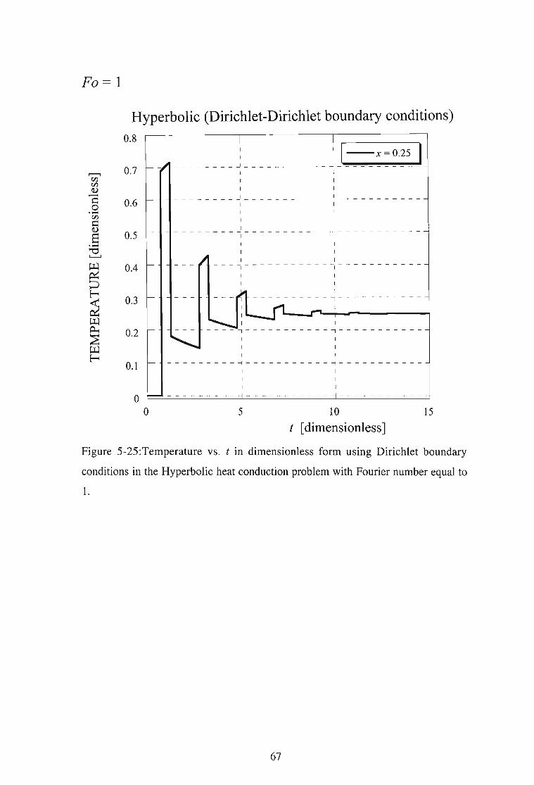
Fo= 1
Hyperbolic (Dirichlet-Dirichlet boundary conditions)
5 10 15
t [dimensionless]
: : I-X=0.25 I- -- - - - --- ~ -- -- - - --- - -~-
I I
I I
I I_ ___ _ _ __ J J _
I I
I I
I I
I I--- - - - - --- -- - ------- - ---- - - - - - - -I II I
I II I
-- -1 - - - - - - - - -- - 1 - - - - - - - - - - -I I
I I
I------- - - - , - --- - ---- - -
I I
I
I I
- -- - , - - - - - - - - - - - , - -- -- - - - - - -I I
I II I
--- - - - - - - ~ -- - - ---- - -- ~- ----- - - -- -
I II I
I I
oo
0.8
,......., 0.7r/)r/)Q)......I::: 0.60.-r/)
I:::Q)
0.58.-"'d~
~ 0.4
~r-- 0.3;2~~ 0.2:E~r--
0.1
Figure 5-25:Temperature vs. t in dimens ionless form using Dirichlet boundary
conditions in the Hyperbolic heat conduction problem with Fourier number equal to
1.
67

Fo= 1
Hyperbolic (Dirichlet-Dirichlet boundary conditions)
0.8
0.6
0.4
0.2
oo
: : \-x=0.51- - - - - - ---j - - - - - - - - - - - --j -
I 1
1 II 1
1 I1 1
I I_ _ _ _ _I _ _ _ _ _ _ _ _ _ _ _ J _ _ _ _ _ _ _ _ _ _ _
1 1
I I
I
I1
1
I I-- - - - , - - - - - - - - - - - ,-- - - - - - - - - -
I 11 I1 I
I 1I 1
1 I
- - - - - - - - - - ~ - -- -- - - - - - - ~ - - - - - - - - - - -I 1
I I1 I
I 1I I
1 I
-- - ------ - - - - - - - - - - - - - - - - - ---- - -
5 10 15
t [dimensionless]
Figure 5-26:Temperature vs. t in dimensionless form using Dirichlet boundary
conditions in the Hyperbolic heat conduction problem with Fourier number equal to
1.
68

Fo = 1
Hyperbolic (Dirichlet-Dirichlet boundary conditions)
--- ---- --- - -- - - - - - - - - - - - - - - - - - - -
: !-x=0.75 IIIIII I
__ -.J .J _
I
I
I
III I
- - - - - -l - - - - - - - - - - - ...j - - - - - - - - - - -
I I
I II I
I I
I II I
-- - - - --- - - ~ ------ - - --- ~ --- -- - ---- -
I I
I II II II II I
-- - - - - ----,- - - - - - - - ---,---- - - - - - - -I I
I I
I I
I I
I I
I I
o
0.4
0.2
0.6
0.8
o 5 10
t [dimensionless]15
Figure 5-27:Temperature vs. t in dimensionless form using Dirichlet boundary
conditions in the Hyperbolic heat conduction problem with Fourier number equal to
1.
69

5.5 Results for the Hyperbolic heat conduction problem subject to a
combination of Dirichlet and Neumann boundary conditions.
5.5.1 Rectangular geometry.
In Figures 5-28 and 5-29 the graphs show the relationship between temperature and x
in a dimensionless form. With Fo = 10-4 in hyperbolic conduction it is shown that the
graphs are almost identical to that of the Fourier conduction. As seen previously with
a small value Fo = 10-4 the wave effects are negligible, so Figures 5-28 and 5-29
show almost identical results as for Fourier conduction in Figure 5-3. Figures 5-30
and 5-31 represent the dimensionless Temperature versus x graphs for Fo = 0.01.
The wave effects are seen as the wave propagates until steady state is reached.
Figures 5-32 to 5-34 represent the dimensionless temperature versus x for Fo = 0.1.
Again the wave effects are seen even better as the Fourier number is increased.
Figures 5-35 to 5-39 represent the dimensionless temperature versus x for Fo = 1. In
these graphs the wave propagation is seen best as the Fourier number is increased
even further. Figure 5-40 shows the dimensionless temperature versus time for Fo =
10-4 . Since Fo = 10-4 is small, the wave effects are not seen and the graph follows the
Fourier solution almost identically. Figure 5-41 shows the dimensionless temperature
versus time for Fo = 0.01, however the Fourier number is still too small for these
effects to be observed. The graph in Figure 5-41 follows the Fourier solution almost
identically. Figure 5-42 shows the dimensionless temperature versus time for Fo =
0.1. The wave effects can only be seen up to approximately a dimensionless time t =
0.63. Figure 5-43 shows the dimensionless temperature versus time graph for Fo = 1.
In this graph the wave effects are seen very clearly. The dimensionless time for the
wave to pass the gap twice is the dimensionless time between a peak and a trough in
the graph shown in Figure 5-43 for x = 1. For all other values of x except x = 0 the
dimensionless time for the wave to pass the gap twice is also represented on the
graph in Figure 5-43 clearly by the peaks and troughs.
70

t = 0.11
t = 0.15
t = 0.19
t= 0.22
I
1
1
I 1 1_ _ _ 1 1 L _
1 1 11 I 1
1 1 I
I 1 1
1 1 1
- - - - - - - I - - - - - - - 1- - - - - - - 1- - - - - - - ~-1 1 I I 1I 1 1 I 1
1 I I 1
1 1 1 11 1 1 I
- - - - - - - I - - - - - - - 1- - - - - - -1- - - -
1 1 11 1 1
1 I 1
1 1
1 1- - ---- - - - --- - - - - -- -I 11 11 11 1
1
- - - - - - _I _ _ _ _
I 11 1
1
I
1
o
0.1
0.2
0.3
0.4
0.5
Fa = 10-4
Hyperbolic (Dirichlet-Neumann boundary conditions)
0.6
,.......,enen(I)......:::o.....en:::(I)
S.....""dL....-l
o 0.2 0.4 0.6 0.8
x [dimensionless]
Figure 5-28 :Temperature vs. x in dimensionless form using a combination of
Dirichlet and Neumann boundary conditions in the Hyperbolic heat conduction
problem with Fourier number equal to 10-4.
71

-4Fa = 10
Hyperbolic (Dirichlet-Neumann boundary conditions)
0.6 0.8
x [dimensionless]
0.40.2
t= 1.0
t= 3.0
oo
t= 0.5
t= 0.7
Figure 5-29:Temperature vs. x in dimensionless form using a combination of
Dirichlet and Neumann boundary conditions in the Hyperbolic heat conduction
problem with Fourier number equal to 10-4 •
72

Fa = 0.01
Hyperbolic (Dirichlet-Neumann boundary conditions)
t = 0.025
0.6 0.8
x [dimensionless]
0.40.2
t= 0.1
t = 0.075
t = 0.025- - - - - - - - - --- -
I
II
I I It = 0.05 _ _ f- - - - - - - l- - - - - - - t- - - - -
I I I
I I I
I I I
I I I-- , - - - -- - ,- - - - - -, - -'----.,....----- I I I
I I I
I I I_ _ _ _ _ _ _ _ _ _ _ __ ~ ~ L
I I I
I I
I I I
__ _ _ _ _: ~ t~~_
I I I
I I I
I I I- - - - - - , - -- ---r - - - - - - r -
I I I
I I
I I
I I----------------I I
I I
II
o
0.1
o
0.2
0.3
0.05
0.15
0.25
0.35
Figure 5-30:Temperature vs. x in dimensionless form using a combination of
Dirichlet and Neumann boundary conditions in the Hyperbolic heat conduction
problem with Fourier number equal to 0.01.
73

Fo = 0.01
Hyperbolic (Dirichlet-Neumann boundary conditions)
1
oo
t= 0.5
t= 0.7
t = 1.0
t= 3.0
0.2 0.4 0.6 0.8
x [dimensionless]
..~........
Figure 5-31 :Temperature vs. x in dimensionless form using a combination of
Dirichlet and Neumann boundary conditions in the Hyperbolic heat conduction
problem with Fourier number equal to 0.01.
74

Fa = 0.1
,
1
1
I
1
-----I :t= 0.32
t = 0.1 1
1
I
t = 0.2 I 1 I- - 1- - - - - - - 1- - - - - - - 1- - --
1 1 1I 1 I1 I 1
1 1 1 1
1 1 1 1- - - - - - 1- - - - - - - 1- - - - - - - 1- - - - - - -
1 1 1
1 1 1 /1 1 1 1 1
1 I 1 1 = 0.32 ' 1- - - - - _ 1- 1 1_ _ _ -; _
1 1 1 1 I1 1 1 1 , 1
1 1 ;, rII I I. .:11 1 1 1= 0.2 ... 1
____ _ -:- - : - _ _ _ _ -:- _ _ / _ -:- .~..L _ 1
1 I I , 1 ... 1
1 1/ I " 11 1 1 1 1="01 1
- - - - - _ 1- _ _ _ _ _ 1 ~ 1_ . _ _ ~ II 1 / I I . · 1I 1 1 ••r I
1 , 1 •• 1 1
I /' I ••- I I1- I .· 1 1_.__.~ ----------- .__.~ - - - - - - - - - -
0.1
o
0.3
0.4
0.2
0.5
Hyperbolic (Dirichlet-Neumann boundary conditions)
0.6
o 0.2 0.4 0.6 0.8
x [dimensionless]
Figure 5-32:Temperature vs. x in dimensionless form using a combination of
Dirichlet and Neumann boundary conditions in the Hyperbolic heat conduction
problem with Fourier number equal to 0.1.
75

Fa = 0.1
t= 0.5
t = 0.41
1
1
1
I 1 1- - - 1- - - - - - - 1- - - - - - - 1- - - - -
t = 0.63 1 I 1
1 I I
1 1 1=~0.63 11 I I / 1I I .. "!
1 I 1 I , ..' 1- - - - - -:- - - - - - -:- - - - - - -:- - - - - -7 - -,:..s": -
I 1 1 ' I ..
1 I 1 / I »"1 I '''~I 1 1/ ...... I1 1 .. I- - - --- �- -- - - - - 1--- -1= 0.5 ~ ..-4I' - - -I - - - - - --
I I _' 1•• - II ~ _.. ro I
1 I , ' 1 = 0.4 1I ·~I.. . II '1._·- I I, ..
- - - - - - : - - ~.:.;••~- - - - - - -: - - - - - - - :- - - - - - - I
~.-.- I I I I;,J........ 1 I I 1
''''...... 1 1 1 I 1.... 1 1 I I
1 1 1 I
Hyperbolic (Dirichlet-Neumann boundary conditions)1
o
0.2
0.4
0.6
0.8
o 0.2 0.4 0.6 0.8
x [dimensionless]
Figure 5-33 :Temperature vs. x in dimensionless form using a combination of
Dirichlet and Neumann boundary conditions in the Hyperbolic heat conduction
problem with Fourier number equal to 0.1 .
76

Fa = 0.1
1
1- t = 1.90I :1 I
- - - - - _ 1- 1 _
I 1 I1 1 1
1 1 II 1 I
1 I 11 I 1 1
- - - - - - 1- _ - - - - - 1- - - - - - - - - - - - - 1- - - - - - -1 1 1 I 1
I 1 1 1 1
I 1 I 1 I
1 I 1 I 1
1 I 1 I 1
I 1 I 1 I- - - - - - 1- - - - - - - - - - - - -1 - - - - - - -1- - - - - - -
1 I 1 I 11 1 I 1 I
1 1 I 1 1
1 I 1 1 1
1 1 1 1 1, 1 I 1 I
- - - - - - 1- - - - - - - 1- - - - - - - 1- - - - - - - I
I 1 I 11 I 1 ,
1 1 1 1
I 1 I 11 1 I I
Hyperbolic (Dirichlet-Neumann boundary conditions)1
o
0.4
0.6
0.2
0.8
o 0.2 0.4 0.6 0.8
x [dimensionless]
Figure 5-34:Temperature vs. x in dimensionless form using a combination of
Dirichlet and Neumann boundary conditions in the Hyperbolic heat conduction
problem with Fourier number equal to 0.1.
77

Fo= 1
Hyperbolic (Dirichlet-Neumann boundary conditions)
0.6 0.8
x [dimensionless]
0.4
.. I..- - - - - --.-........
I .... 1
- - - _ 1- _~ _I 1 .. 1
t = 1.0 I.... 1.or ~-:-- - - ~,~~:- - - - -/ -:
1 _, " 1 , 1
: t = 0.75: / :- - - - - I ~"- - - - - - 1- , - - - - - I
" ~ 1
.. 1 ~ ),
1 , .... 1 t = 0.5 1-- - 1- - - - ,- - - 1- - - - - ---7-
1 ....# I / 1
0.2
0.8
0.7,...-,0000(])........
0.6I=:0.....00I=:(]) 0.5a.....
"'0'---'
~0.4
~~ 0.3~~p.. 0.2~~~
0.1
00
Figure 5-35:Temperature vs. x in dimensionless form using a combination of
Dirichlet and Neumann boundary conditions in the Hyperbolic heat conduction
problem with Fourier number equal to 1.
78

Fo= 1
0.6 0.8
x [dimensionless]
0.40.2
t > 1.25
( =1.5
(= 1.75
(= 2.0
1
1
I 1 I
_ _ 1 J _ _ - f-=-2-.O- - - - -I 1 "-I _1 1 ~ / 11 1 _", I
1 1 ~", 1-. - - 1- - - - - - -j - - - - ..... t- - - ~ - - -
I 1 I ", /.
1 I ~"" 1
I 1 t> 1 5 /" II I _ ..- I
- - - - - - - - - - - - - 1- - - - - - - , - - - ]1'-' - - - - - I
I I"' "" 1 11 ,,~I /" 1 1
1 1 1 f = 1.25 I I- - - - - - I- - - - - - - 1- - - - - -i,"-- - - - - - -I- - - - - - -
1 1 ,,0"1 1 1
I .- I I I1 1,,0 I 1 I
I .. 0" I I I- - - - - - I - - 0~ 1 - - - - - - I - - - - - - T - - - - - - I
1 y"" 1 1 1 1
1 1 I 1 1
I 1 I IL 1 -l .L _
I 1 1 1 I
1 I 1 I 1
1 1 I 1 1
1 1 I 1 I
oo
0.4
0.6
0.2
0.8
Hyperbolic (Dirichlet-Neumann boundary conditions)
1.4
1.2
Figure 5-36:Temperature vs. x in dimensionless form using a combination of
Dirichlet and Neumann boundary conditions in the Hyperbolic heat conduction
problem with Fourier number equal to 1.
79

Fa = 1
t = 2.5t = 2.25
t = 2.5
t = 2.75
t = 3.0
0.2
o
0.4
0.8
1.2
0.6
Hyperbolic (Dirichlet-Neumann boundary conditions)1.4
,---,tiltilQ)
""2o.-till=:Q)
S:.aL......J
o 0.2 0.4 0.6 0.8
x [dimensionless]
Figure 5-37:Temperature vs. x in dimensionless form using a combination of
Dirichlet and Neumann boundary conditions in the Hyperbolic heat conduction
problem with Fourier number equal to 1.
80

Fa = 1
t = 3.25
t = 3.5
t = 3.75
o
0.4
0.6
0.2
0.8
Hyperbolic (Dirichlet-Neumann boundary conditions)1.2
.........,enenQ)
Co.....enl=:Q)
S....."'0L.....J
o 0.2 0.4 0.6 0.8
x [dimensionless]
Figure 5-38:Temperature vs. x in dimensionless form using a combination of
Dirichlet and Neumann boundary conditions in the Hyperbolic heat conduction
problem with Fourier number equal to 1.
81

Fo= 1
Hyperbolic (Dirichlet-Neumann boundary conditions)1
0.6 0.8
x [dimensionless]
0.40.2
t = 15.0
t= 5.0 I ~
I ."1""I ".
1 ""I ""I .,,-
-- - -- - - - - - - - - - - - - - - - - - - - - - - - - - - -I I I .".I I .'I I ••- I
I 1 ••- I
I I " II I I ••••• I
_ _ ___ _ L L ,~ ~ _
I I ~." II 1 ."1 I
"I I " 1I I •••• I
I I ••" I
- - - - - - ~ - - - - - - 1 ~"~" ~ ~ _
"1 ". I I.I "" 1 1 1I _,,- I 1 I
I ••- I 1 I
1 ."" 1 I II ••- I I I
- - - - - - "- - - - - - r - - - - - - T - - - - - - .,. - - - - - -
••"1 I
" I1
I
I
I
oo
0.2
0.4
0.6
0.8
Figure 5-39:Temperature vs, x in dimensionless form using a combination of
Dirichlet and Neumann boundary conditions in the Hyperbolic heat conduction
problem with Fourier number equal to 1.
82

Fo = 10-4
Hyperbolic (Dirichlet-Neumann boundary conditions)1.5
5
I
II
II.._..._ ...II
I
I
I--or-------II
I
I
I-i-·_·_·_·
3 4
t [dimensionless]
21o
I X=O II I
I X = 0.25 II I
I x = 0.5 II I
I x=0.75 II II x = 1 I
I IL ~ _ _ _ _ __ x=lI I I II I II I I
I I II I I I
I I _ •••_I.··_···_··x = 0.75I j,•. - I I
I ."""'l I II •• I I I
I / I I I
I I I I I 0r- - : - - - 1'" - - ,;;.-.----1--- - ---- - -,.x = .5I I __1- - " 1 I
I , I I I
I ,. • I I I
I ,',,' I I I
I I I I 025I : , \.. • _ • - • - • -I" - • - • - • - ·,x = .I," .",. II ,,I,· 'r=0,I. ;I' ~'I'II -- -- - -o
0.5
Figure 5-40:Temperature vs. t in dimensionless form using a combination of
Dirichlet and Neumann boundary conditions in the Hyperbolic heat conduction
problem with Fourier number equal to 10-4•
83

Fo = 0.01
Hyperbolic (Dirichlet-Neumann boundary conditions)1.5
IIIII
,.......... _ ...II
II
I'-""1-- - ---
I
II
I..~._._._.-I
III
I
x=O
x = 0.25x=0.5x = 0.75
x=l
IIII
II
I
II
------:---~-...----T-------r:x = 1III
I I I
I _ •••_l. .•_ •.. _ .•lX = 0.75~... I I
•• I I I• I I
I I I I
• I I I 05- L - - - r - - - - "~"------iX =" .- .- I'" ........ - - I I '
• , I I I
: ,' 1 I I
I' I I II • I I ._._._J_·_·_·_·.Jx = 0 25I :,' .«: 'l"'.- I I'
I I'.' I I I.' , I I., • I I
." I I,.o
0.5
,......,IZlIZl(1).......:::o......IZl:::(1)
8......"'0'---'
o 2 3 4
t [dimensionless]
5
Figure 5-41 :Temperature vs. t in dimensionless form using a combination of
Dirichlet and Neumann boundary conditions in the Hyperbolic heat conduction
problem with Fourier number equal to 0.01.
84

Fa = 0.1
Hyperbolic (Dirichlet-Neumann boundary conditions)1.5
I x= O I
1 1
I X = 0.25 1
1 I
1 x= 0.5 1,........,u:l 1 Iu:l
1 X = 0.75 111)........ I Il=l 1 x = l 10..... I Iu:l - - - - - - - 1- - x = ll=l11) 1 I 1
S I I I
..... 1 1 1
"'d 1 1 I 1 1L......I
I I I 1I
~1 1 _ •• ·_···,.....···_···.....,x = 0.75 -·r·-···-···..1 • 1 1 1 1
~ 1 / I 1 I 1
~ 1 . 1 1 1 I•
~1 • 1 1 1 1
0.5I _l_ - _1- - - ~_._!....._--_ --.!.x = 05 1------------I ,. _ ..... - I I · I
~ 1 . ,I I I 1
~ I,
I , I I I I
::E 1 · ,1 I I 1· I
~ I · I I I I
~ I I " ....I_ . _ . _ . _ . _ I· _ · _ · _ · _ · .l.x = 0.25 . J_._._._.1 ., • 1 1 1 1
1: , ,
I I I 1,,' ,.1 1 1 x = O I
I ·, . 1 1 :t 1• I ,• I • 1 1 1
0 - - - - -0 2 3 4 5
t [dimensionless]
Figur e 5-42:Temperature vs. t in dimensionless form using a comb ination of
Dirichlet and Neumann bou ndary conditions in the Hyperbolic heat conduct ion
problem with Fourier number equal to 0.1.
85
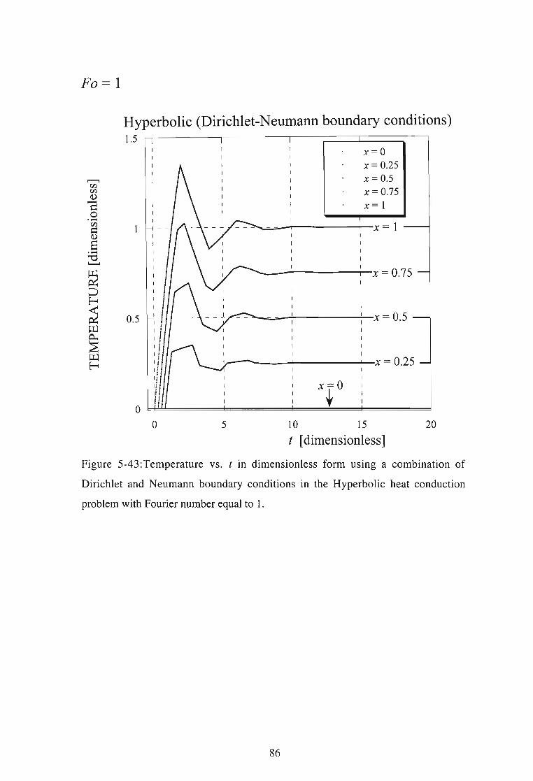
Fo= 1
Hyperbolic (Dirichlet-Neumann boundary conditions)1.5
0.5
o
I
II
I
I
I
I
II
:-/I I
I II !I fdI !II iii lIiiIi jI::
Ii
o 5
x =Ox = 0.25x= 0.5x = 0.75
x=1
"""-..:;;..__--r--------t-x = 1
'----.--------r-x = 0.75
"'--.........---"--------:...-.x = 0.5
.__-__--l------.l---x = 0.25
x=Ot
10 15
t [dimensionless]20
Figure 5-43:Temperature vs. t in dimensionless form using a combination of
Dirichlet and Neumann boundary conditions in the Hyperbolic heat conduction
problem with Fourier number equal to 1.
86

5.5.2 Cylindrical geometry.
Figure 5-44 shows the dimensionless temperature versus r for Fa = 10-4
• The wave
effects are not seen due to the small Fourier number. The graph in Figure 5-44
follows almost identically to the Fourier solution shown in Figure 5-5. Figure 5-45
shows the dimensionless temperature versus log(r) for the same Fa = 10-4
• Again this
graph follows almost identically to the Fourier solution shown by Figure 5-6. Figures
5-46 and 5-48 show the dimensionless temperature versus r for Fa = 0.01. Figures 5
47 and 5-49 show the dimensionless temperature versus log(r) for the same Fa =
0.01. The graphs in Figures 5-46 to 5-49 show the wave propagation until steady
state is reached. Figures 5-50 and 5-52 show the dimensionless temperature versus r
for Fa = 0.1. Figures 5-51 and 5-53 show the dimensionless temperature versus
log(r) for Fa = 0.1. The graphs in Figures 5-50 to 5-53 show the wave propagation
until steady state is reached. Figures 5-54, 5-56 and 5-58 show the dimensionless
temperature versus r for Fa = 1. Figures 5-55, 5-57 and 5-59 show the dimensionless
temperature versus log(r) for Fa = 1. The wave propagation is evident in Figures 5
54 to 5-59. With Fa = 1 the wave effects are seen most clearly as it takes longer to
reach steady state . Figure 5-60 shows the dimensionless temperature versus time for
Fa = 10-4 . The wave effects are not seen in the graph in Figure 5-60 due to the small
value for the Fourier number. The graph in Figure 5-60 follows almost identically the
Fourier solution shown in Figure 5-7. Figure 5-61 shows the dimensionless
temperature versus time for Fa = 0.01. The wave effects are only seen up to an
approximate dimensionless time t = 0.1. For this reason the wave effects are not seen
in Figure 5-61 very clearly. Figure 5-61 follows the Fourier solution almost
identically since the wave effects are only seen for small values of dimensionless
time. Figure 5-62 shows the dimensionless temperature versus time for Fa = 0.1. The
wave propagation can be seen more clearly in Figure 5-62 and is best seen in Figure
5-63. Figure 5-63 shows the dimensionless temperature versus time for a Fourier
number Fa = 1. The dimensionless time for the wave to pass the gap is represented
by equation (4-60) tL = (1- rw).JFa . For Fa= 1, the dimensionless time to pass the
gap is approximately tL
::::: 1 (because rw
= 0.002 «1). In Figure 5-63 the
dimensionless time for the wave to pass the gap twice is represented by the
dimensionless time between peaks which is approximately t = 2. This corresponds to
equation (4-60) where twice tL is 2. For larger values of r shown on the graph in
87

Figure 5-63 the peaks are a little harder to see but the dimensionless bouncing period
still corresponds to that of equation (4-60).
t = 0.02
t = 0.05
t = 0.10
t = 0.20
t = 2
0.80.60.40.2
1
1
I1 1 1
- - - - - - T - - - - - - I - - - - - - - I - - -
I I 1
1 I I1 I 1
- - - - - - .!. - - - - - - -' - - - - - - _ 1- _ _1 1 1
1 I 1I 1 1I 1 1 1
- - - - - - -+ - - - - - - ~ - - - - - - - I - - - - - - - 1- - - - - -I 1 1 I
1 1 1 1
1 1 I 1
fl' I I 1 1~a~ - - - - """[ - - - - - - I - - - - - - - I - - - - - - - ,- - - - - -
"a. 1 1 1 1
'" • 1 I I 1\',\ I 1 1 I_ 1 ~ 1 1 _
1 1 1 1
I I 1
\' '. I 1 1 I
\ ',', a'a 1 1 1- - - - - ~.;i - ... - - - - - - - - - - 1- - - - - - - 1- - - - - -
, " I ...... '" 1 1 1"". ... ......." .,.. -.... ,. . . ....... I
.. L -.. ---- 1. I~ -. --. ........- - - - - - I __.._~__"·I"._._.~"' ~...o
o
0.01
0.002
0.004
0.006
0.008
0.012
Hyperbolic (Dirichlet-Neumann boundary conditions)
0.014
r [dimensionless]
Figure 5-44:Temperature vs. r in dimensionless form usmg a combination of
Dirichlet and Neumann boundary conditions in the Hyperbolic heat conduction
problem with Fourier number equal to 10-4.
88
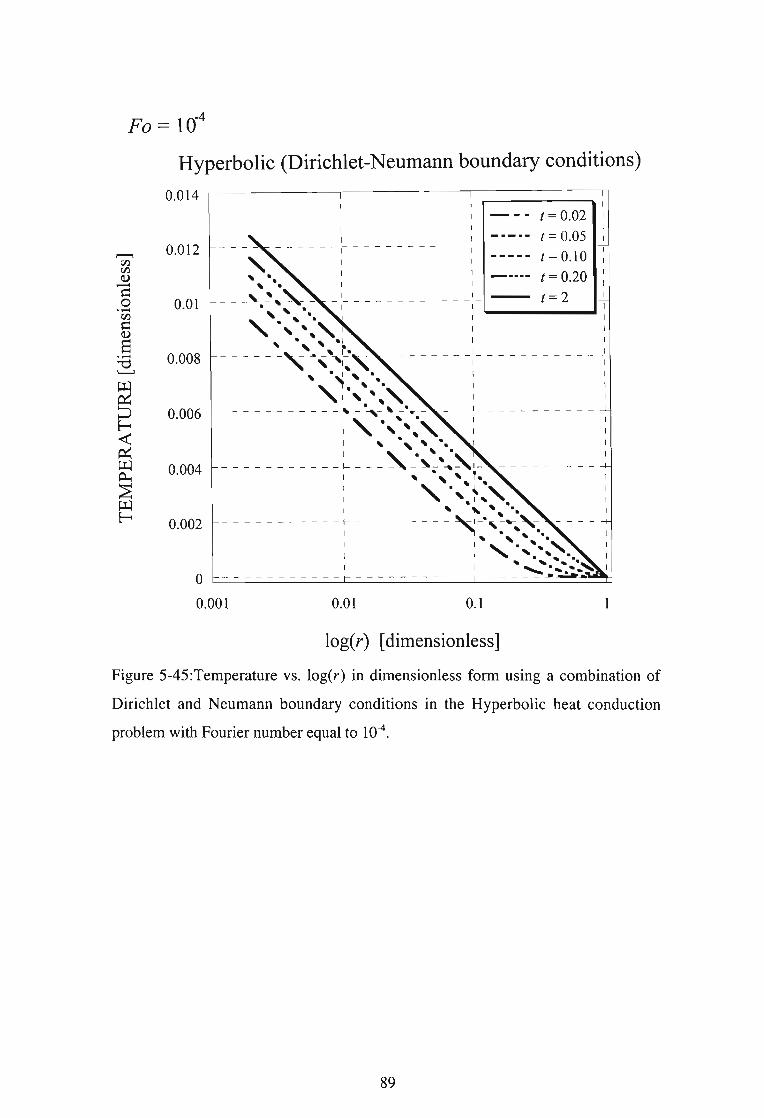
Fa = 10-4
Hyperbolic (Dirichlet-Neumann boundary conditions)
0.014t = 0.02
t = 0.05t = 0.10
t = 0.20t = 2
0.1
1 1
1 11 1
I 1- - 1- - - - - - - - - - - - 1-' I 1
" '. I 1" • 1 I
- - -'- ~ 'lr~- _ 1 :_• ". I '"- ..
, ,,'. 1 -
" " "" I 1" • ".~ 1
- - - - - -"' .." -,,:~,, - - - - - - - -:- - - - - - - - - - -
" ,~" '. 1~ 1 , • I
' I" '" 1- - - - - - - - - - - , - ~_ " _ . r - - - - 1- - - - - - - - - - -I" ."', 11 , " 1. '
I '" "'. 11 ~. " •
- - - - - - - - - - - I- - - - - , - ~ - '""",~ I -1 " '," r,1 ~ ',',."1 '.1" .1 " "",'.
- - - - - - - - - - - ~ - - - - - - - - - ~_', ~~,,~.
'" ,,'" .1 1 '- • "'""I I "' '." -,.. " .1 I """'lo - - --- -- - --- - - - - - - - - -- - - --- - - ~ ..
0.001 0.01
0.01
0.002
0.004
0.006
0.008
0.012
log(r) [dimensionless]
Figure 5-45 :Temperature vs. log(r) in dimensionless form using a combination of
Dirichlet and Neumann boundary conditions in the Hyperbolic heat conduction
problem with Fourier number equal to 10-4.
89

Fa = 0.01
Hyperbolic (Dirichlet-Neumann boundary conditions)
0.012
t = 0.1
t = 0.05
t = 0.0251
II
1 1 1___ _ _ _ L L L __
1 I 1
1 1 1I I I
I I 11 1 I I
- - - - - - ~ - --- - - ~ - - - - - - ~ - - --- - + - - - - - -
I 1 I I
I I 1 I
1 1 1 11 1 I 1I I 1 I
- - - - - - 1- - - - - - - I - - - - - - r - - - - - - T - - - - - -
1 1 1 1
I I I 1
I I I I
I 1 1 I
1 1 I 1- --- - - --- - - - - - - - - - - - - - - - - - - - - - - -I I I I
I 1 1 1
1 1 1 1
1 1 I II I 1 I1 L L 1- _
I I I
I I I
1 1 1
1 1
1
o
0.01
0.002
0.004
0.006
0.008
o 0.2 0.4 0.6 0.8
r [dimensionless]
Figure 5-46:Temperature vs. r in dimensionless form using a combination of
Dirichlet and Neumann boundary conditions in the Hyperbolic heat conduction
problem with Fourier number equal to 0.01.
90

Fa = 0.01
Hyperbolic (Dirichlet-Neumann boundary conditions)
0.012
t = 0.1
t = 0.05
t = 0.025
0.1
log(r) [dimensionless]
0.01
I
1
I
1 1
-- - - - ~- - - -- - - - - - - ~I 1I 1'- ...1 1
I 11 1
~ -- -- - - -- ---;- - - --- -- ---
1
1
1
I1
--- -- - , ---- - - - - ---1
1
I
1
- -- - - - - - - - ~ - - - - -,~~ - - ~- - - - - - - - - - -1 , I
,. 1,1 , ', 1
I , ~
- - - - - - - - - - .J - - - - - - - - - - -v ~.-1 ~ ,
I I' "1 I ,.
1 I'I 1 ,".
- - - - - - - - - - - - - - - - - - - - - - - - - ....- ~
,---., -,, -,, -.- - - - - - - - '\-, .
, '.1,' I.,- - - - - - - - - - ,'- -', -
1 , •
I ,'.I ,1 ,.
o0.001
0.01
0.002
0.004
0.006
0.008
Figure 5-47:Temperature vs. log(r) in dimensionless form using a combination of
Dirichlet and Neumann boundary conditions in the Hyperbolic heat conduction
problem with Fourier number equal to 0.0 1.
91
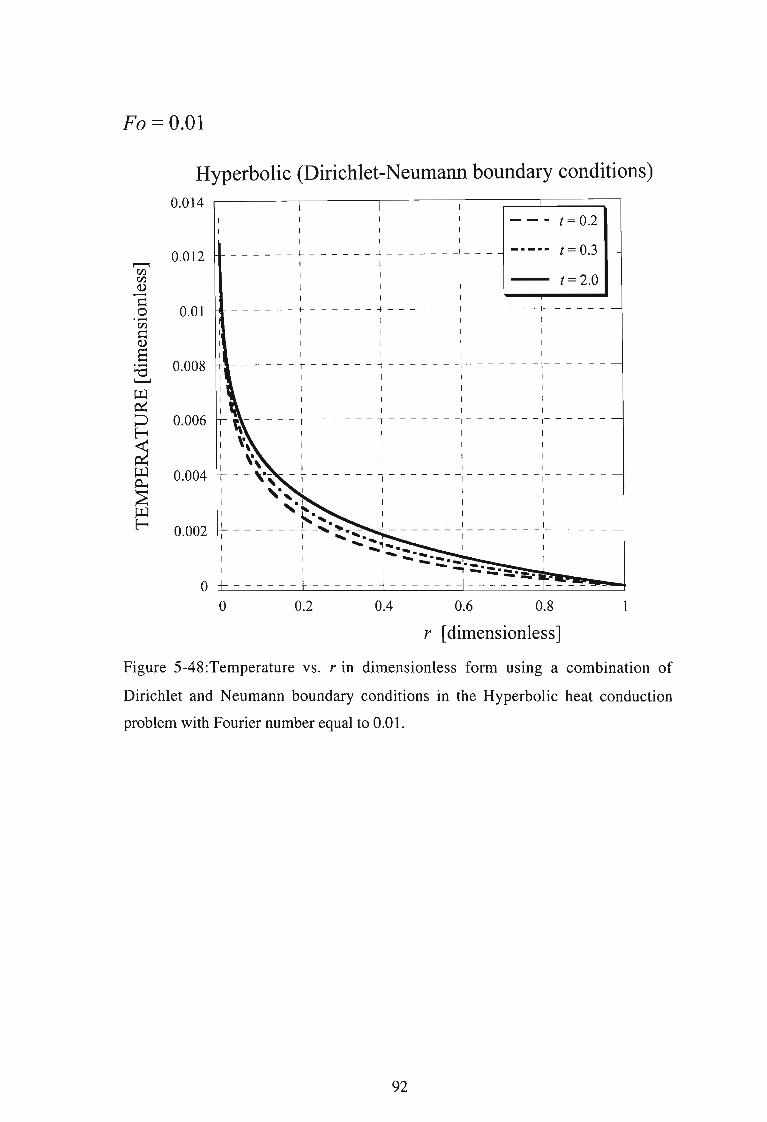
Fa = 0.01
Hyperbolic (Dirichlet-Neumann boundary conditions)
0.014
t= 2.0
t= 0.3
t = 0.2
0.6 0.8
r [dimensionless]
0.40.2
I
1
1 1 \_ _ _ _ __ L J ~ _
1 1 \
\ \ I
1 1 11 1 1
- - - - - - ~ - - - - - - ~ - - - - - - -1- - - - - - -1- - - - - -
1 1 I 11 1 I I1 I 1 I
1 1 \ 1- - - - - - I - - - - - -; - - - - - - - 1 - - - - - - - 1- - - - - -
I I I I
1 1 I I
1 1 1 11 1 1 1
tJ- - - - - r - - - - - - I - - - - - - -1 - - - - - - - \- - - - - -
"\ 1 1 I 1
\\ 1 1 1 1,. 1 1 1 1
\ 1 1 \ 1- - ", - T - - - - - - "I - - - - - - - I - - - - - - - 1- - - - - -
", I I I I.... 1 I 1 I"' ro. 1 1 1
i' 1 1 1- - - - - - - - !Io r - - - - - - - - - - - - - - - - - - - - - -
1 .... ....... 1 \
1 - _,....... I I- ...I 1 II I --'-::'-:.- ... _ ...
-_·Y~~~-J
oo
0.01
0.002
0.004
0.006
0.008
0.012
Figure 5-48:Temperature vs. r 10 dimensionless form using a combination of
Dirichlet and Neumann boundary conditions in the Hyperbolic heat conduction
problem with Fourier number equal to 0.01.
92

Fa = 0.01
Hyperbolic (Dirichlet-Neumann boundary conditions)
0.014
t= 0.3
t = 2.0
t= 0.2II
I I
- - - - - - - 1- - - - - - - - - - - - I-I II I
I I,. I I
- - - - - - - ~ - - 1- - - - - - - - - - - - 1- - - - - - - - - - -
", I I
", 1
'"~ Ii' I- - - - - - - - - - - I -~~ - - - - - - - - 1- - - - - - - - - - -
I ", II ~ . I
I "" I_ _ _ _____ _ _ _ 1 ~~'L 1 _
I ", II ,. II , I
I '.,- - - - - - - - - - _ 1- ,~"""' _
I I .....1 I ""
I I ",
I I ",- - - - - - - - - - -1 - - __ - 1- - - - - ,.,
1 I ,",
I I ~ ,I I "'-"I I
0.01
0.002
0.004
0.006
0.008
0.012
o0.001 0.01 0.1
log(r) [dimensionless]
Figure 5-49:Temperature vs. log(r) in dimensionless form using a combination of
Dirichlet and Neumann boundary conditions in the Hyperbolic heat conduction
problem with Fourier number equal to 0.01.
93

Fa = 0.1
Hyperbolic (Dirichlet-Neumann boundary conditions)
0.014
0.012,.......,enen(l)........I=lo 0.01......enI=l(l)
S:.a 0.008"--'
0.006
0.004
0.002
oo 0.2 0.4
( == 0.1
t > 0.2
(==0.316
I__ __ __ L _
I
I
I
0.6 0.8
r [dimensionless]
Figure 5-50:Temperature vs. r in dimensionless form using a combination of
Dirichlet and Neumann boundary conditions in the Hyperbolic heat conduction
problem with Fourier number equal to 0.1.
94

Fa = 0.1
Hyperbolic (Dirichlet-Neumann boundary conditions)
0.014
t > 0.1
(= 0.2
(=0.316
0.1
log(r) [dimensionless]
0.01
III
_ __ __ __ 1 _I
I., I
" • I I_ __ _,~~ __ l ~ _
, I I
". I I
" '. I~ I
____ _ __ _ ~ -1' , 1. _
~ • Il' , I
I " • I,I ". I_ _ _ _ _ _ _ _ _ _ .1 , _ ". .1 _
I , I
I ". II ,,'. II ,
- - -- - - - -- - ~ -- -- - -- - , - ~
I " '.I I ,
I , "
I I" "-- -- - - -- - - ~ - --- - -- - -- - + -- - - -
I I ,',
I I ' "I I \',I I •_ _ __ _ _ _ _ _ _ _ _ _ _ _ _ _ _ _ _ _ _ _ _ _ _ .L_~o
0.001
0.01
0.002
0.004
0.006
0.008
0.012
Figure 5-51 :Temperature vs. log(r) in dimensionless form using a combination of
Dirichlet and Neumann boundary conditions in the Hyperbolic heat conduction
problem with Fourier number equal to 0.1.
95

Fo = 0.1
Hyperbolic (Dirichlet-Neumann boundary conditions)
0.014
0.012
0.01
0.008
~o 0.006~
;2g: 0.004
~~
~ 0.002
oo 0.2 0.4
t> 0.1
t> 0.2
( =0.316
(= 1.894
0.6 0.8
r [dimensionless]
Figure 5-52:Temperature vs. r in dimensionless form using a combination of
Dirichlet and Neumann boundary conditions in the Hyperbolic heat conduction
problem with Fourier number equal to 0.1.
96

Fa = 0.1
t= 0.1
t= 0.2
t= 0.316
t = 1.894
0.1
log(r) [dimensionless]0.01
O c-- ---'---- --'- _
0.001
0.002
0.01
0.004
0.006
0.008
0.012
Hyperbolic (Dirichlet-Neumann boundary conditions)
0.014
Figure 5-53:Temperature vs. log(r) in dimensionless form using a combination of
Dirichlet and Neumann boundary conditions in the Hyperbolic heat conduction
problem with Fourier number equal to 0.1.
97

Fa = 1
Hyperbolic (Dirichlet-Neumann boundary conditions)
0.014
t = 0.25
t = 0.5
t = 0.75
t = 0.998
I
I
I_ _ _ _ _ _ L L L __
I I
I I
I II I
_ _ __ __ 1 L L __ '- 1...,
I I
I II II I I I
__ _ _ _ _ L L L ~ _I I I I I II I I I I I
I ~' I I I II , I I I I I\~ _ _ _ _ 1_ _ _ _ _ _ _ L _ _ _ _ _ _ L _ _ _ _ _ _ ~ _ _ _ _ _ _
I "', I I I II I I I I I I
I " \~ I I I I
I \ \ I. I I I I-\_ ,'~I- ------~ ------~ ------~ ------\ "T.. I I I
J. " I I I\. l' -.. I I. " ......__ __ , _ ~ _ _~ - -b~ - L ~ _
• I ' I......... I~ ' I ......... I I
I , .,...
I , I .... '"I I I ..... I .......__ __ _ _ _ _,_~ • __-1._ '.o
0.01
0.002
0.004
0.006
0.008
0.012
o 0.2 0.4 0.6 0.8
r [dimensionless]
Figure 5-54:Temperature vs. r in dimensionless form using a combination of
Dirichlet and Neumann boundary conditions in the Hyperbolic heat conduction
problem with Fourier number equal to 1.
98
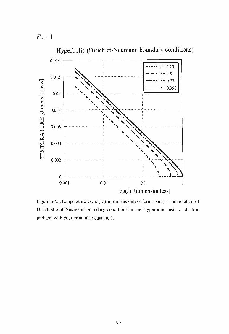
Fo= 1
Hyperbolic (Dirichlet-Neumann boundary conditions)
0.014t = 0.25
t = 0.5
t = 0.75
t = 0.998
0.1
log(r) [dimensionless]
0.01
II
~ I :- - " -'. - - - - - I - - - - - - - - - - - I,'~~ I I
" I I, , '. I I
- - - ~'-. _ _,'~ 1 ~ '- " -j
'. "'. I, "'~ I" I, . I
__ _ _ _ __ __ .. ..1 --.- ..1 _
-. ,~ II , , '. II . • I
I '. '" I_ _ _ _ _ _ _ _ _ _ -.1 _ _ _ "",-_ _ ~ L. _ -.1 _ _ _ _ _ _ _ _ _ _ _
I • • I
I '.' "I " .. .I .. 1 •
____ _ _____ -.1 ~ . -~-~
I , I ,'.I • I _"'"~
I 't '"'I I " v >,_ __ __ _ _ _ _ _ -1 -I _ J _ _ ~~
I I ' ·
I I '\ "',I I ' \I I \ '.
- - -- - -- --- - - - - - - - - - - - - --- ~ -_.j_.o0.001
0.01
0.002
0.004
0.006
0.008
0.012
Figure 5-55:Temperature vs. log(r) in dimensionless form using a combination of
Dirichlet and Neumann boundary conditions in the Hyperbolic heat conduction
problem with Fourier number equal to 1.
99

Fo= 1
Hyperbolic (Dirichlet-Neumann boundary conditions)
0.014
-
t = 1.996
t = 1.75
t = 1.25I
II
___ _ __ L L _I
I
II
_ _ ___ _ L L 1 _I 1
1 II I
I I I_ _ _ _ _ L L L ~ _
I I I I
I I I 1
~\ I I I I
\" I I I I_ ~ _ _ _ 1_ _ _ _ _ _ _ L _ _ _ _ _ _ L _ _ _ _ _ _ ~ _ _ _ _ _ _
,', I I I I
, • I I 1 I
'. 1 I I I
" I I I_~.~ L L ~ _
I ",," 1 I I~ I I I
'~""' I I II I I
- - - - - - 1- - - - - - - .- -~ ---.10 - - - - - - ~ - - - - - -I I ......... I ............ I
I I ~ I1 I ,..,
I I
o
0.01
0.002
0.004
0.006
0.008
0.012,.......,enenQ)..-co.-enCQ)
8.-"'0L.......J
o 0.2 0.4 0.6 0.8
r [dimensionless]
Figure 5-56:Temperature vs. r in dimensionless form using a combination of
Dirichlet and Neumann boundary conditions in the Hyperbolic heat conduction
problem with Fourier number equal to 1.
100
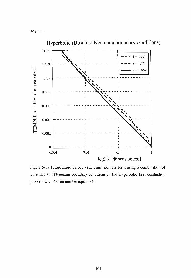
Fo= 1
t = 1.25
t = 1.75
t = 1.996
0.01 0.1
log(r) [dimensionless]
I
I
I
- - - - - - - -- - -1 - - -I
II
o0.001
0.01
0.002
0.004
0.006
0.008
0.012
Hyperbolic (Dirichlet-Neumann boundary conditions)
0.014
,.......,r:r.Jr:r.JQ)......I=:o.....r:r.JI=:Q)
8....."'d.........
Figure 5-57:Temperature vs. log(r) in dimensionless form using a combination of
Dirichlet and Neumann boundary conditions in the Hyperbolic heat conduction
problem with Fourier number equal to 1.
101

Fo = 1
Hyperbolic (Dirichlet-Neumann boundary conditions)
0.014
0.012
0.01I - - - - --I
II ,.I ,
0.008I
IIII
0.006I
0.004
0.002
oo 0.2 0.4 0.6
t = 2.994
t = 3.992
t = 20.958
0.8
r [dimensionless]
Figure 5-58:Temperature vs. r in dimensionless form using a combination of
Dirichlet and Neumann boundary conditions in the Hyperbolic heat conduction
problem with Fourier number equal to 1.
102
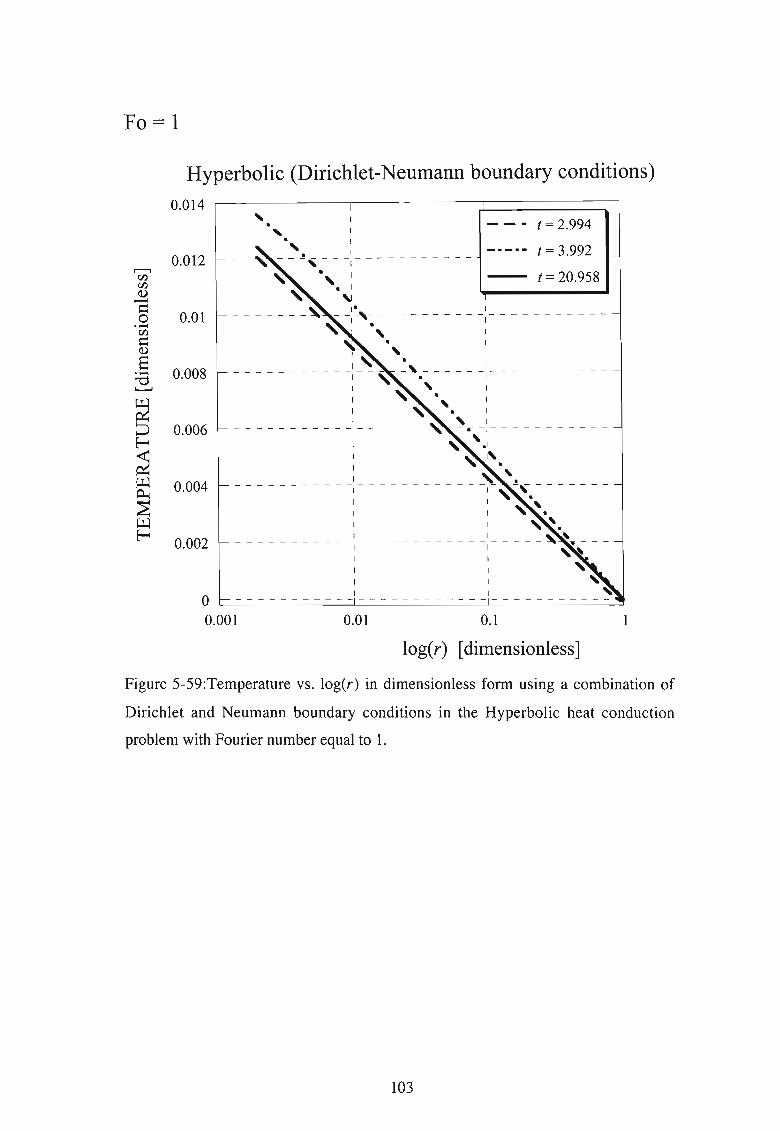
Fo = I
t = 2.994
t = 3.992
t = 20.958
"
0.002
0.004
0.006
o - --- ---- -- - ------- - - --- - - - - - - --- --0.001 0.01 0.1
log(r) [dimensionless]
Hyperbolic (Dirichlet-Neumann boundary conditions)
0.014
0.012,...--,mmCI).......I=:o 0.01.....mI=:CI)
S..... 0.008'"d~
Figure 5-59:Temperature vs. log(r) in dimensionless form using a combination of
Dirichlet and Neumann boundary conditions in the Hyperbolic heat conduction
problem with Fourier number equal to 1.
103
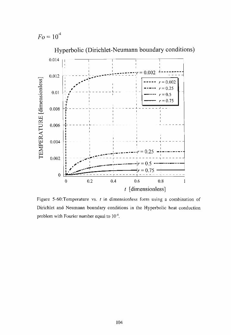
-4Fa = 10
Hyperbolic (Dirichlet-Neumann boundary conditions)
-
-
r = 0.002
r = 0.25
r= 0.5
r = 0.75
III
0.014 I I I II I I I
I I I I
f-:- : .....-~ ~~---::-_·-- :r = 0.002 j -: -_-.:- : -=--_- ~0.012 I .1.0-- I I
I " I I II " I I
I ,' 1 I I
0.01 f-:-/ - - - -- ~ ------; - ----- ~ -I ' 1 I I
I : I 1 I
I I I I I
0.008 1'- - - - - - - l- - - - - - - 1-. - - - - - - .i - - - - - - J - - - - - - -~ I 1 I II I I I I
I I I I I, I I I I
0.006 f-l- - - - - - - I- - - - - - - j... - - - - - - + - - - - - - -4 - - - - - -I I I I I
I I 1 I I
I I I I I
I I I I
0.004 rt- - - - - - - t- - - - - - - t- - - - - - - 1- - - - - - - -t - - - - - - -I I I I I
I I I I I
I I I - ••r=025 ,-+-·_·_·_··I I .'-----1------- I • I
0.002 M---~~;,-;!-~ ----~ --~.~~~.~r-~05-. :. l.:. ~. =-= .~ .~I' I .......--, •• - I • I". • •• ...,..... 1 1 075 ......I -tI . ." I Ir . Io I..· r r T I
o 0.2 0.4 0.6 0.8
t [dimensionless]
Figure 5-60:Temperature vs. t in dimensionless form using a combination of
Dirichlet and Neumann boundary conditions in the Hyperbolic heat conduction
problem with Fourier number equal to 10-4 •
104

Fa = 0.01
-
-
-
Hyperbolic (Dirichlet-Neumann boundary conditions)0.014 I I I I I
I I I I II I I I I
I I I = 0 002 .l - - - J - - - - - - - - -0.0 12 f-l - - - - - - J - - .._ .. __- _Of r . _I- - - - - - I - - - - - -
I .. l." .. .. I 1 r---.....I- - - ----.
: " ..... : : : r=0.002I ' I I I • r= 0.25
0.01 ~ -;,~-- --~-- - - - - -: - -- - --- : -- • 0I ' I I I r = .5I : I I I r =0.75I , I I 1
0.008 [-u -- - - - - --l - - - -- - - I - - - - - - - I - -I' I I I I
: ' I I I I, I I I 1, 1 I I I
0.006 H-- - - - - ~ - - - - - - -I - - - - - - - 1- - - - - - - 1- - - - - - -~ I I I I• I I I I
I I 1 I I
I I 1 I
0.004 rt - - - - - - -t - - - - - - - 1 - - - - - - - 1- - - - - - -1- - - - - - -
I I I I I
I I I I I
I I __'r = 0.25 ._1__ -------+---------I I .... -. I I I
0.002 H - - - - -...-. ",,---.:- - - - - I - - - - - - - 1- - - - - - - 1- - - - - - -I .... I '
r= 0 5 ~ -l.... _
.,. I ........--, • 1 I
I. _••.....,...-- I - 0 75 I I
I' ." 1r . I Io • ., I - I - I
o 0.2 0.4 0.6 0.8
t [dimensionless]
Figure 5-61 :Temperature vs. t in dimensionless form using a combination of
Dirichlet and Neumann boundary conditions in the Hyperbolic heat conduction
problem with Fourier number equal to 0.01.
105
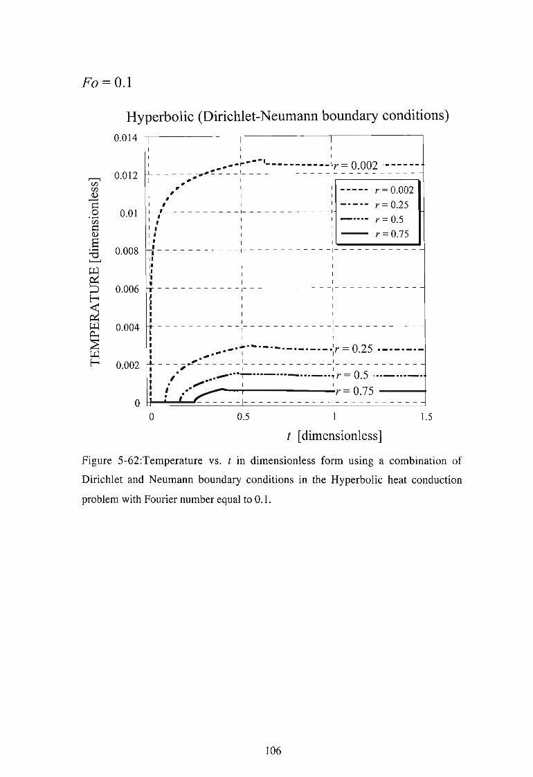
Fa = 0.1
-
r = 0.002
r = 0.25
r = 0.5
r = 0.75
Hyperbolic (Dirichlet-Neumann boundary conditions)
0.014 1 I I1 I I
1 I 1
1 ............ ,.. ......... ,---- - - --- -- Lr = 0.002 .- -- ---0.012 ..L - - - - - ~ - - _ 1- - - - - - - - - - - _ 1- - - - - - - - - - --
I ,," I I ,....---------".I " I 1 _
I " I I1 I I 1 _._.-
0.0 1 I+- -' - - - - - - - - - - 1- - - - - - - - - - - - II .' I I _ ••• -1 , I 1
I ' I I -I ' I 1'- ...
0.008 -tl - - - - - - - - - - - 1- - - - - - - - - - - - 1- - - - - - - - - - - -
I' I II' I I
I: I 1It I I0.006 r-.- - - - - - - - - - - - 1- - - - - - - - - - - - 1- - - - - - - - - - - -
i : :, I I, I I0.004 It - - - - - - - - - - - 1- - - - - - - - - - - - 1- - - - - - - - - - - -
I I II ""."".""·~·"·-·-·-·_._._.:r= 0.25 ._.-._.-0.002 +---,~:. -----:------------:- ----------
I ,. ..".....•••,.-•••_ •.• _ •••_ •. , r = 0.5 ... _ ..._.I . ". 1 I
I·· r=075o I ~ • ,. I· .1 '
o 0.5 1
t [dimensionless]
1.5
Figure 5-62:Temperature vs. t in dimensionless form using a combination of
Dirichlet and Neumann boundary conditions in the Hyperbolic heat conduction
problem with Fourier number equal to 0.1.
106

Fo = 1
r = 0.002
r = 0.25
r = 0.5r = 0.75
•••.... 1 I I I
.. I ' 1'.. I 1, I I : ·r= 0.002 ,•••••: - - - -t~-~- - ~ - - - - - r - - - - - r - - - - - r - - - -
1 " I " I 1 II I I 1 I II I I I I II I 1 1 1 I
I I I I I III I I 1 1II 1 I I I
I: I I I I_ _ _ _ _ 1 1 L, l--_._!!!""!!!'_ "'!!_!"'!_!!!""!!!'_'!!!"!!!!"!""'''!!'''''~
I I I I II I I I I
I I I I I
I I I I I
- --- - ~ -- - - - ~ - - - - - ~ - -- - -~ -- - - - ~ - - - -
I I I I I
I I I I I1 I I I I
1 I I I I- - -,.~ 1- - - - - - 1- - - - - - 1- - - - - - 1- - - - - - 1 - - - -
,. '. 1 1 I I I
• \ ~." I 1, . ,. ..... 'T'·-·_·-·.,·-r=025··_·_·• 1\ ._1 I -._1 .I I~,.·l.~ :-·~·~ ---:------:- -----:------:- ----, • I' ,.".··j.....···_.. · .....···--··· ....... ···-r = 0.5 --_..I!! I ........ I I I .
II: r=0.75• l-- l-- l-- l-- L _o
0.01
0.002
0.004
0.006
0.008
0.012
Hyperbolic (Dirichlet-Neumann boundary conditions)0.014
o 2 4 6 8 10
t [dimensionless]
12
Figure 5-63:Temperature vs. t in dimensionless form using a combination of
Dirichlet and Neumann boundary conditions in the Hyperbolic heat conduction
problem with Fourier number equal to 1.
107

5.6 Results of the SEED (Synthetic Experimental Emulation Data) method.
When evaluating the thermal conductivity by applying the Transient Hot Strip
method and using the Fourier Law one obtains from equation (4-11) the following
solution for the dimensional temperature TL• (t) at x = 1
[TL*(t)-Tc' ] = Iq~.1 L.[1+ f(t)]app
where
(5-1)
(5-2)
and for initial conditions of T = 0 the values of C are evaluated and expressed ino n
the form
C = _ 8n (2n + 1)2n2
which following substitution into equation (5-2) yields
From equation (5-1) the thermal conductivity can be evaluated in the form
(5-3)
(5-4)
(5-5)
where the temperature difference [TL* (t) - Tc. ] is represented by the recorded
experimental data and the value of the wall heat flux \qLI is evaluated from the Joule
heating of the hot strip in the form IqL\ =iV/ A ' strip , where A ' strip =d.l, is the heat
transfer area of the hot strip , with I. being the length of the strip and d. the depth of
the hot strip .
A method of Synthetic Exp erimental Emulation Data (SEED is applied now to
evaluate the de viation between Fourier and hyperbolic thermal conduction.
According to the SEED method one assumes that the data expressed by
[TL* (t)- Tc. ] represent a different than Fourier conduction solution, in this case a
hyperbolic thermal conduction solution. Then the values of [TL* (t)- Tc• ] obtained
from the hyperbolic solution expressed by equations (4-40) and (4-49) are substituted
in equation (5-5) to yield
108

kapp [1+ f(t)]-c= [1+h(t)]
(5-6)
where k is the apparent thermal conductivity obtained from the Fourierapp
conduction solution while k is the actual thermal conductivity that corresponds toact
data that follow the hyperbolic conduction, and where f(t) can be evaluated from
equation (5-4) while h(t) is evaluated from equation (4-39). The ratio between the
two will provide the deviation of the apparent thermal conductivity from the actual
one.
All the results presented here apply to the dimensional time range that was evaluated
in section 2.2 to be consistent with the Transient Hot Wire method.
Figure 5-64 shows the thermal conductivity ratio versus time for Fa = 10-4 for copper
in Ethylene Glycol for rectangular geometry. It is seen that even with a small Fa =
10-4 when the wave effects are small, at short values of time there is an
overestimation of the thermal conductivity when using Fourier conduction values.
Figure 5-65 shows the thermal conductivity ratio versus time for Fa = 10-4 for carbon
nanotubes in oil for rectangular geometry. The results are similar to that in Figure 5
64 only slightly higher. This means that the overestimation with carbon nanotubes in
oil is higher then that of copper in Ethylene Glycol. Figure 5-66 shows the thermal
conductivity ratio versus time for Fa = 10-3 for copper in Ethylene Glycol for
rectangular geometry. The overestimation of the thermal conductivity at t = 5s is
approximately 150%. Figure 5-67 shows the thermal conductivity ratio versus time
for Fa = 10-3 for carbon nanotubes in oil for rectangular geometry. For carbon
nanotubes in oil the overestimation of the thermal conductivity at t = 5s is
approximately 160%. Figure 5-68 shows the thermal conductivity ratio versus time
for Fa = 0.01 for copper in Ethylene Glycol for rectangular geometry. With the
increase in the Fourier number the wave effects are more noticeable. For this reason
the overestimation of the thermal conductivity is greater. At a time t = lOs in Figure
5-68 the overestimation of the thermal conductivity is approximately 250%. Figure
5-69 shows the thermal conductivity ratio versus time for Fa = 0.0 I for carbon
nanotubes in oil for rectangular geometry. At a time t = lOs in Figure 5-69 the
overestimation of the thermal conductivity is approximately 260%. For a cylindrical
geometry similar derivations apply. When evaluating the thermal conductivity by
applying the Transient Hot Wire method and using the Fourier Law one obtains from
109

equation (4-47) the following solution for the dimensional temperature Tw' (t) at
where
f{t)= I,cn exp[ - t3; tJn=O
(5-7)
(5-8)
and for initial conditions of To= 0 the values of en are evaluated by using equations
(4-47) and (4-45)
From equation (5-7) the thermal conductivity can be evaluated in the form
(5-9)
where the temperature difference [Tw• (t)- Te. ] is represented by the recorded
experimental data and the value of the wall heat flux qo' is evaluated from the Joule
heating of the hot wire in the form qo' =iV/2nrw.l. , where 2nrw.l. is the heat
transfer area of the hot wire, with I. being the length of the wire l is the electric
current flowing through the wire and V is the voltage drop across the wire.
A method of Synthetic Experimental Emulation Data (SEED is applied now to
evaluate the deviation between Fourier and hyperbolic thermal conduction.
According to the SEED method one assumes that the data expressed by
[Tw.{t)-Te. ] represent a different than Fourier conduction solution, in this case a
hyperbolic thermal conduction solution. Then the values of [Tw• (t)- Te. ] were
derived by using the hyperbolic solution presented in equations (4-48) evaluated at
r = rw to yield
kapp [ -rwIn(rw) + f{t)Jkact = [-rwln(rw)+h{t)J
(5-10)
where kapp is the apparent thermal conductivity obtained from the Fourier
conduction solution while kact is the actual thermal conductivity that corresponds to
data that follow the hyperbolic conduction, and where f{t) can be evaluated from
equation (5-8) while h(t) is derived from the hyperbolic solution (4-48) evaluated at
r = rw • The ratio between the two will provide the deviation of the apparent thermal
110

conductivity from the actual one. Figure 5-70 shows the thermal conductivity ratio
versus time for Fo = 10-4 for copper in Ethylene Glycol for cylindrical geometry.
Comparing Figure 5-70 to 5-64 shows that the overestimation in cylindrical
geometry is lower then that in the rectangular geometry. Figure 5-71 shows the
thermal conductivity ratio versus time for Fo = 10-4 for carbon nanotubes in oil for
cylindrical geometry. Again the overestimation of the thermal conductivity is less in
cylindrical geometry then in rectangular one. Figure 5-72 shows the thermal
conductivity ratio versus time for Fo = 10-3 for copper in Ethylene Glycol for
cylindrical geometry. The overestimation of the thermal conductivity at t = 5s is
approximately 105%, which is 45% lower then that in rectangular geometry. Figure
5-73 shows the thermal conductivity ratio versus time for Fo = 10-3 for carbon
nanotubes in oil for cylindrical geometry. The overestimation of the thermal
conductivity at t = 5s is approximately 110%, which is 40% lower then that in
rectangular geometry. Figure 5-74 shows the thermal conductivity ratio versus time
for Fo = 0.01 for copper in Ethylene Glycol for cylindrical geometry. The
overestimation of the thermal conductivity at t = lOs is approximately 125%, which
is again lower then that in rectangular geometry. Figure 5-75 shows the thermal
conductivity ratio versus time for F 0 = 0.01 for carbon nanotubes in oil for
cylindrical geometry. The overestimation of the thermal conductivity at t = lOs is
approximately 130%, which is again lower then that in rectangular geometry. In
Figures 5-74 and 5-75 the overestimation in thermal conductivity at time t = 5s is
approximately 155% and 160% respectively. This shows that even though there is a
big difference in the overestimation of thermal conductivity between rectangular and
cylindrical geometry it is still significant and of the same magnitude as the
experiments predict the enhancement in thermal conductivity.
111
Cu in Ethylene Glycol
65432
1
I1
1
1
1- - - - - - 1- - - - - - r
1 I
1 1I 1
: : ( 1+ f )l( 1+ h ) I_ _ __ __1 ~ 1 l ' _
1 I1 1
1 11 1 1 1 1
- - -1- - - - - - ~ - - - - - - 1- - - - - - ~ - - - - - -1- - - - --1 1 1 1 1
1 1 1 I 11 I 1 1 1
1 1 1 1 I- - - - - -I - - - - - - I - - - - - -1 - - - - - - I - - - - - - 1- - - - - -
1 1 1 1 11 1 1 1 I1 1 1 I 1
__1 L 1 L _ - - - - - 1- - - - - -
1 1 1 1 1
1 1 1 I 1I I 1 1 11 I 1 1 11- - - - - - r - - - - - - I - - - - - - r - - - - - - I - - - - - -
I 1 1 11 1 1 1
1 I 1 1_ __ _ L I L I _
1 I 1 11 I 1 I1 1 1 I
1 1 1- - - - - 1- - - - - - r - - - - - - 1- - - - - -
1 1
1
1.8
1.7
~
....s::: 1.6
+......."-" 1.5...........
~+....... 1.4"-"II
ti 1.3..J:<.<:J<,
~ 1.2~
1.1
10
time [8]
Figure 5-64: Thermal conductivity ratio vs. time in dimensional units for Cu in
Ethylene Glycol in rectangular geometry for a Fourier number equal to 10-4.
112

0-4
Fo= 1 Carbon Nanotubes in Oil
-- ( 1 + f) /( 1 + h ) Ii i
1
I
I- - - - - - 1- -
1
1
I__ __ __ 1 L _
1
I
I
1
1
11
1- - - - - -- - - - -- - - - l-- - - - - --- - - - r - -- - -
I 11 I
1 1_ __ _ _ _ _ _ _ _ _ _ L 1 L _
1 1
1 II 1
1 1 1 1 I_ _ 1 L ~ 1 1 _
I 1 1 I 1
1 I 1 1 I1 I I 1 1
I 1 1 1 1
- 1- - - - - - ~ - - - - - + - - - - - -1 - - - - - - 1- - - - - -1 I I I 11 1 1 I 1
1 1 1 1 I
1 I I 1 1- --- -- r - -- -- ~- - -- - ~ - - - - -- r- - -- -
I 1 II 1 11 I 1I I I- - - r - - - - - - - - - - - 1- - - - - - 1- - - - - -
I 1 11 I 1
I I1 I- --- --- -- ---- -- -- -1 11 1
1.1
1.2
1.3
1.4
1.5
1.6
1.7
1.8
II
1o 1 2 3
time [s]
4 5 6
Figure 5-65 : Thermal conductivity ratio vs. time in dimensional units for Carbon
Nanotubes in Oil in rectangular geometry for a Fourier number equal to 10-4 ,
113

-3Fo= 10 Cu in Ethylene Glycol
-- ( 1 + f )/( 1 + h )
- - - - - - - - 11
1
I
I1
I
- -- - -- - -~--- -- -- -- r -- -- - - --~ - - - - -- - -
1 I II 1 11 1 11 1 1
-- - ---- , - --- - --- - r - -- --- - - ,- - - - - - --1 I 11 1 1
1 1 11 1 1-- - - - - - 1-- - - - -- - - 1 ----- - - - 1---- -- --1 1 I
I I 1
1 I 1_ _ _ _ _ _ _I L I _
I 1 1
I I 1
1 1 1I 1 1
- - - - - ~ - -- -- - - - - ~ - - - -- -- - ~ - - - - - - - -1 1 I
I I 1
1 1 I1 1 I
--- , - - - - - - - -- ,- - - - - - - - , - - - - - - - -1 I 1
1 1 I
I 1 1
1 1- - -- -- -- 1 -- --- -- - 1 - -- -- - --
I I
I
4
2
3
5
1.5
2.5
3.5
4.5
II
1o 5 10 15 20
time [s]
Figure 5-66: Thermal conductivity ratio vs. time in dimensional units for Cu In
Ethylene Glycol in rectangular geometry for a Fourier number equal to 10-3•
114

-3Fo= 10 Carbon Nanotubes in Oil
-- ( 1 + f)/( 1 + h ) II
1 11 I1 11 I- - - - - - - I - - - - - - - - - 1- - - - - - - - - I - - - - - - - -I I 1
1 1 1I 1 1
___ _ ___ ~ L ~ _1 1 1I I 1
1 1 11 1 1
- - - - - -- ~ - - - - - - - - - ~ - - - - - - - - ~ - - - - - - --1 1 1I 1 1
1 1 I
1 1 1--- - - - , - - -- -- - - - r---- -- - - , -- -- --- -
1 I
1 I
1 11 1- - - - - 1 - - - - - - - - - , - - - -- -- - - - - -- - - -1 1
1 11 1
_ _ _ J _ _ _ _ _ _ _ _ _ 1_ _ _ _ _ _ _ _ _ _ _ _ _ _ _ _ _
1 11 11 1
I_ _ _ _ _ __ L J _
1 1
1
_ __ __ _ _ _ J _
1
1
1
4
2
3
5
1.5
2.5
3.5
4.5
II
1o 5 10 15 20
time [s]
Figure 5-67: Thermal conductivity ratio vs. time in dimensional units for Carbon
Nanotubes in Oil in rectangular geometry for a Fourier number equal to 10-3•
115
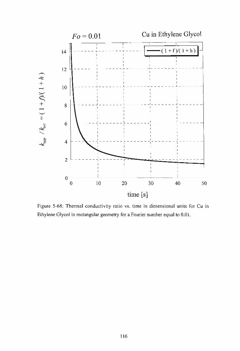
Fa = 0.01 Cu in Ethylene Glycol
I
--- - -- ~ - - - - - -~-~-:-~----~~~~~~~~~~~jI
1
- - - - - - ~ - - - - - - - ~ - - - - - ~ ( 1 + 0/( 1 + h ) I1 1 11 1 11 1 1 1
- - - - - - ~ - - - - - - - ~ - - - - - - - 1- - - - - - - ~ - - - - - -
1 1 1 11 I I 1
1 1 1 1I I 1 1
_ _ _ _ __ ...J l- 1 - ...l - - - - - -
I 1 1 1
1 I I I1 1 1 1
I 1 I 1__ _ __ .J L 1 ...I _
1 1 1 1I 1 1 1
1 I I I1 I I I
_ _ _ _ _ J L 1 J _1 I I I1 1 1 1I 1 1 1
I 1 1 I
1 1 1 1- - -I - - - - - - - I - - - - - - -1- - - - - - - I - - - - - -
1 1 1 11 1 I
1 1 1I I
---- ---- 1- -----1
I
I
2
4
6
8
10
12
14
II
oo 10 20 30 40 50
time [s]
Figure 5-68: Thermal conductivity ratio vs. time in dimensional units for Cu in
Ethylene Glycol in rectangular geometry for a Fourier number equal to 0.01.
116

Fa = 0.01 Carbon Nanotubes in Oil
504030
-- ( 1 + O/( 1 + h )
2010
I I- - - --- ~- -- - -- - r -- - - -
I I '----------...I I
I II I I I
-- - - --~ - -- - -- - r - --- - - , --- - ---r ------
I I I I
I I I I
I I I I
I I I I
- - --- -~ ---- - --~- - - ---~ - -- - - - - ~ - --- - -
I I I I
I I I I
I I I I
I I I I- - - - - ~ - - - - - - - 1- - - - - - - ~ - - - - - - - ~ - - - - --
I I I I
I I I I
I I I I
I I I I
- - - - - - ~ - - - -- - -~ - - - - -- ~- - - - - - - ~ - - - - - -I I I I
I I I I
I I I I
I I I I_ _ ~ L ~ L _
I I I I
I I I
I I I
I I I 1___ ___ ~ L __ _ _ L _
I I
I I
I I
I I
o
2
4
o
6
8
10
12
14
II
time [s]
Figure 5-69: Thermal conductivity ratio vs. time in dimensional units for Carbon
Nantubes in Oil in rectangular geometry for a Fourier number equal to 0.01.
117

-4Fa = 10 Cu in Ethylene Glycol
54321
: ( 1 + [)/( 1 + h ) I1 1
-- - - - - -- --- - 1- -- - ----- - - -- - , --- - - -1 I1 I
1 I
1 1 1 1- - - - - - -j - - - - - - - t- - - - - - - - 1- - - - - - - -j - - - - - -
1 1 1 II 1 1 1
1 I 1 I1 1 1 1
_ __ ~ L 1 ~ _
1 I 1 I
1 1 1 I1 1 1 11 1 1 1
1 1 I I- - - -I - - - - - - - I" - - - - - - - 1- - - - - - - "I - - - - - -
I 1 1 1
1 1 1 11 I 1 1
I 1 1 1- - -j - - - - - - - t- - - - - - - - 1- - - - - - - -t - - - - - -
1 1 I I1 1 1 1
I 1 1 11 I I I~ L 1 ~ _
I 1 1 1I I I
1 1 11 1 I
I I
o
1.1
1.2
1.3
1.05
1.15
1.25
1.35
II
time [s]
Figure 5-70: Thermal conductivity ratio vs. time in dimensional units for Cu in
Ethylene Glycol in cylindrical geometry for a Fourier number equal to 10-4,
118

1.35
-4Fa = 10 Carbon Nanotubes in Oil
II
1.3
1.25
1.2
1.15
1.1
1.05
I
: ( I + f )/( I + h ) I_ _ __ ...1 !... ...1_ - - - - -
I I
1 1
1 11 1
I 1 1 1- - - I - - - - - - - I - - - - - - -, - - - - - - - I - - - - - -
1 1 1 11 I I I1 1 1 11 1 1 1
- - - -l - - - - - - - I- - - - - - - - 1- - - - - - - -l - - - - - -
1 1 1 1
1 1 1 II I I 1
1 1 1 1__ J L 1 J _
1 , I ,
1 1 1 1
1 1 1 1I 1 1 I
1 I I I- I - - - - - - - I - - - - - - - 1- - - - - - - I - - - - - -
1 1 1 1
I I I I1 1 1 11 1 1 1
-l - - - - - - - I- - - - - - - -1 - - - - - - - -1 - - - - - -
I I I
1 1 1 11 1 1 1I 1 1 I
_ _ _ _ _ _ .J =_-:_""r_~_~_~_~_ '!!O' ......J ~
o I 2
time [s]
3 4 5
Figure 5-71 : Thermal conductivity ratio vs. time in dimensional units for Carbon
Nanotubes in Oil in cylindrical geometry for a Fourier number equal to 10-4.
119

-3Fo= 10 Cu in Ethylene Glycol
II
3
2.5
2
1.5
1
- - - - - - - - ~ - - - - - - - - - 1- - - - - - - - - ~ - - - - - - - -
: : I (1 + f)/( 1 + h ) I1
1
1
1
1 1 1
-- - - - - - - ~ - - - - - -- - - ~ -- - - - - -- ~ - - - --- - -
1 1 I1 I 1I I 1
1 1 I
I I 1
I 1 I
1 I I
I I 1
- - - - - - - ~ - - - - - - - - - ~ - - - - - - - - ~ - - - - - - - -
1 1 I
1 I 1
I 1 1
1 1 I
1 I 1
I I 1
1 1 1
1 1 I- - - - - - I - - - - - - - - -1- - - - - - - - - I - - - - - - --
1 1 1
1 1 I
I I 1
I 1 11 1 11 1 1
I 1 11 1
o 5 10
time [s]
15 20
Figure 5-72: Thermal conductivity ratio vs. time in dimensional units for Cu in
Ethylene Glycol in cylindrical geometry for a Fourier number equal to 10-3•
120

-3Fa = 10 Carbon Nanotubes in Oil
1412108642
I 1 1 1 1 1 1- - - - r - - - - r - - - - T - - - - I - - - - 1- - - - -1 - - - - -1 - -
I \ I I I I: : : : ( 1 + 0/( 1 + h ~I I I I I I I1 1 1 11 1 1 I
1 1 1 1I I I I 1 I I
- - - 1- - - - - r - - - - T - - - - I - - - - - \ - - - - - 1- - - - - I--
1 1 1 \ 1
1 1 1 1 1
1 1 1 1 1
I I 1 I I
I 1 I 1 I1 1 1 1 11 I 1 \ 11 1 1 1 1
- - - I - - - - I - - - - - - - - - I - - - - - 1- - - - -I- -
I I 1 I II 1 I 1 1
1 1 1 I 1
1 I 1 1 I1 1 I 1 1
1 1 1 I 1
I I 1 1 I1 1 I 1 1
- 1 - - - - 1 - - - - - - - - - I - - - - - 1- - - - - ,- -
1 1 1 1 1
1 1 1 I 1
" 1 I II 1 1 I
1 I ' 11 1 I 1
, 1 1
1
o
2
3
1.5
2.5
'-"II
time [s]
Figure 5-73: Thermal conductivity ratio vs. time in dimensional units for Carbon
Nanotubes in Oil in cylindrical geometry for a Fourier number equal to 10-3•
121

Fa = 0.01 Cu in Ethylene Glycol
5040302010
: ( 1 + 0/( 1 + h ) II I j
- --- - - - -- - - - - -1 - - - - - - - 1 - - -- -- - 1 - - - - --1 I 1
I I II I I I
- - 1 J 1 L _I I I I
1 I I I
I I I I1 I 1 1
- - - - - - - 1- ...J .1 L _
I I I I
1 I I I
1 I I I
1 I I I- - - - - - - 1- - - - - - - ...j -l- l-. _
1 I 1 I
1 I 1 I
1 I I 11 I 1 I
- - - - - - - I - - - - - - - -j - - - - - - _ + I- - - _
1 I I I1 I I I
1 I I I
I I I I- - - - - - 1- - - - - - - ~ - - - - - - - T - - - - - - - r - - - - - -
1 1 I II 1 I I
1 I I I
1 I I I- - - - - I - - - - - - - I - - - - - - - T - - - - - - - r - - - - - -
1 I I 1I I I 1
1 I 1
o
2
3
5
6
7
4
1
8
9
II
time [s]
Figure 5-74: Thermal conductivity ratio vs. time in dimensional units for Cu in
Ethylene Glycol in cylindrical geometry for a Fourier number equal to 0.01.
122
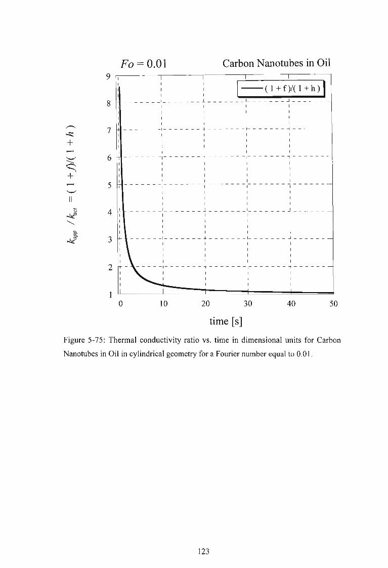
Fa = 0.01 Carbon Nanotubes in Oil
5040302010
1 I (l+f)/(I+h)1__ _ __ _ _ 1 -l L ...J - - - - - -
I I 1 11 1 1 I1 1 1 11 1 1 1
_ _ _ _ _ __ 1_ - - - - - - + - - - - - - -1- - - - - - - -l - - - - - -
1 1 1 II I I 1
1 1 1 11 1 1 1
- - - - - - - 1- - - - - - - T - - - - - - - 1- - - - - - - I - - - - - -
1 1 1 I
1 I I 11 1 1 I
1 I 1 1- - - - - - - 1- - - - - - - T - - - - - - - 1- - - - - - - I - - - - - -
1 I 1 11 I I 1I 1 1 I
_ _ _ _ _ _ _ 1 .1 1 J _1 I I 1I 1 I I
1 I 1 11 1 I 1
- - - - - - 1- - - - - - - ~ - - - - - - -1- - - - - - - ~ - - - - - -1 1 1 1
I I I 11 1 1 I
1 1 1 1- - - - - 1- - - - - - - T - - - - - - - 1- - - - - - - , - - - - - -
1 1 1 I
1 1 1 II 1 1
o1
2
3
4
5
6
7
8
9
II
time [s]
Figure 5-75: Thermal conductivity ratio vs. time in dimensional units for Carbon
Nanotubes in Oil in cylindrical geometry for a Fourier number equal to 0.01.
123

A comparison between the wire temperatures evaluated via Fourier and Hyperbolic
solutions is presented in what follows. Figure 5-76 shows the dimensionless Wire
Temperature vs. t in dimensional units for Ethylene Glycol using a combination of
Dirichlet and Neumann boundary conditions for Fourier and Hyperbolic heat
conduction problems with a Fourier number equal to 10-3for copper in Ethylene
glycol. Figure 5-76 shows that for the time window of 10 seconds the Fourier heat
conduction displays a linear result, and for the hyperbolic heat conduction the result
looks almost linear. Only at times past 10 seconds the hyperbolic solution turns
toward the Fourier solution and shows a non-linear curve. Therefore, when using the
transient hot wire method for a time window of up to 10 seconds to prevent
convection a hyperbolic solution may seem linear and may be confused with the
Fourier solution. Figure 5-77 shows the dimensionless Wire Temperature vs. t in
dimensional units for Ethylene Glycol using a combination of Dirichlet and
Neumann boundary conditions for Fourier and Hyperbolic heat conduction problems
with Fourier number equal to 10-3 for carbon nanotubes in oil. This graph in Figure
5-77 shows a similar result to the one in Figure 5-76. Again for the time window of
10 seconds the hyperbolic heat conduction solution looks linear and can be mistaken
for the Fourier solution when using the transient hot wire method. Figure 5-78 shows
the dimensionless Wire Temperature vs. t in dimensional units for Ethylene Glycol
using a combination of Dirichlet and Neumann boundary conditions for Fourier and
Hyperbolic heat conduction problems with Fourier number equal to 0.01 for copper
in Ethylene glycol. As the Fourier number is increased the wave effect becomes
more apparent, however with Fa = 0.01 the hyperbolic solution for the time window
of 10 seconds still may pass for linear. For this reason it may be mistaken for the
Fourier solution when using the transient hot wire method. Figure 5-79 shows the
dimensionless Wire Temperature vs. t in dimensional units for Ethylene Glycol using
a combination of Dirichlet and Neumann boundary conditions for Fourier and
Hyperbolic heat conduction problems with Fourier number equal to 0.01 for carbon
nanotubes in oil. The same effect is seen here as in Figure 5-78. From Figure 5-79
one can draw the same conclusions as from Figure 5-78. Figure 5-80 shows the
dimensionless Wire Temperature vs. t in dimensional units for Ethylene Glycol using
a combination of Dirichlet and Neumann boundary conditions for Fourier and
Hyperbolic heat conduction problems with Fourier number equal to I for copper in
Ethylene glycol. Figure 5-81 shows the dimensionless Wire Temperature vs . t in
124
dimensional units for Ethylene Glycol using a combination of Dirichlet and
Neumann boundary conditions for Fourier and Hyperbolic heat conduction problems
with Fourier number equal to 1 for carbon nanotubes in oil. Figures 5-80 and 5-81
show that even when the Fa = 1, at a time window of 10 seconds the hyperbolic
solution still may seem linear. This may be mistaken when using the transient hot
wire method for a Fourier solution. The significance of the conclusions discussed
above about Figures 5-76 to 5-81 is that when looking at the results from the
transient hot wire method a Fourier solution is used, even though a hyperbolic
solution might be the one revealed. This may cause an overestimation of the thermal
conductivity ratio presented in the graphs shown in Figures 5-64 to 5-75.
125

-3Fo = 10 Cu in Ethylene Glycol
0.008
0.007 - - -- - - --- ---- - - - - -- - - - - - -- - -- -- - - - - -
.'."".'.""- - - -'- - - - - -
"",.,.,.,.,_ ____ __ _ ~~J - - - - - - - --- - ---
.',
--Fourier r = 0.002_. _ •• Hyperbolic r = 0.002
-- - - - - - - - - - - - - -- --r-----------~
-- - - --- -- - -- - ---- -'-- - - - - - - - ......I-J
-,-'- -- -- - -- .~ - -- -- - -- - - --- -- -- -- - -- -- - -
,.'.',,.
0.002
0.003
0.004
0.005
0.006
0.001
o1 10
time [s]
Figure 5-76: Temperature [dimensionless] vs. t in dimensional units for Ethylene
Glycol using a combination of Dirichlet and Neumann boundary conditions for
Fourier and Hyperbolic heat conduction problems with Fourier number equal to 10-3•
126

0.008
-3Fo= 10 Carbon Nanotubes in Oil
0.007
0.006
0.005
0.004
0.003
0.002
0.001
- - - -- - -- - - -- - - - --- -- --- - -- - ------- - -
.'.'.'- - ~ .. ~ - - - , .
.',.'
- - - - -- -- -,~~- - - - - - - - - - - -- -, ..',.,.
- - - - - - - - - - .-!!'- - - - - - - - - - - - - - - - - - - - - - - - -,.'.,.,..... .!.~ - - - - - - - - - - - - - - -.---- - - - - - - - - - ,,-1
-- Fourier r = 0.002_. _. - Hyperbolic r = 0.002
- - - - - - - - -- - - - - - -- - '-- - - - - - - _ .....I-j
0 1.--- - - - - - - - - - - - - - - - - - - - - -
1time [s]
10
Figure 5-77: Temperature [dimensionless] vs. t in dimensional units for Carbon
Nanotubes in oil using a combination of Dirichlet and Neumann boundary conditions
for Fourier and Hyperbolic heat conduction problems with Fourier number equal to
10-3•
127

0.008
Fa = 0.01 Cu in Ethylene Glycol
--Fourier r = 0.002_. _. - Hyperbolic r = 0.002
0.007
0.006
0.005
0.004
0.003
0.002
0.001
o1
- - - - - - - - - - - - - - - --- - - - --- ------- -- ---
.'- - --- - - -- - - - --- - - - ---- - - - --~.,.,, ..,-- - - - - - - - - - - --- - - -- - - - - - - -~ ~ -- - - - - - -.,.,.,,---- - - -- ---- -- --- 7 J
- - - - - - - - - - - - - - - - -,.
___ _ - - - - .~.~- - - - - - -.---------------,H.'.'.'.'.'
- - - - - - - - - - - - - - - - - _.'-- - - - - - - _ .....L.j
10time [s]
Figure 5-78: Temperature [dimensionless] vs. t in dimensional units for Ethylene
Glycol using a combination of Dirichlet and Neumann boundary conditions for
Fourier and Hyperbolic heat conduction problems with Fourier number equal to 0.01.
128

Fa = 0.01 Carbon Nanotubes in Oil0.008
0.007 - - - - - - - - - - - - - - - - - - -- - - - - - --- --- - - - - -
-------- ---- ------'-- - - - - - - - .....,--Fourier r = 0.002_. _ .• Hyperbolic r = 0.002
,.- -- -- - -- - - - -- -- - - - - - -- - -- - --~ - - -- - - -.,.,.
.',- -- - - - - -- - - - - -- - - - - , ~- - - - - - - - - - -- - - -, .
.'- - - - - - - - -,.~- - - - - - - ,....--------------.,.-\,.,.,.,..-.
0.001
0.002
0.003
0.004
0.005
0.006
o1 10
time [s]
Figure 5-79: Temperature [dimensionless] vs. t in dimensional units for Carbon
Nanotubes in oil using a combination of Dirichlet and Neumann boundary conditions
for Fourier and Hyperbolic heat conduction problems with Fourier number equal to
0.01.
129
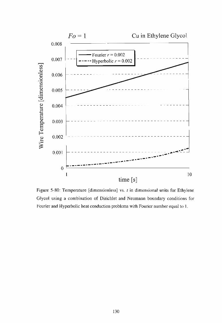
0.008
Fo= 1 Cu in Ethylene Glycol
0.007
0.006
0.005
0.004
0.003
0.002
0.001
o1
-- Fourier r = 0.002_. _. - Hyperbolic r = 0.002
.-.---- - ---- - - - -- - - - -- -- - ---- -- --- - -~ - -
--..- ..---------------------.--------10
time [8]
Figure 5-80: Temperature [dimensionless] vs. t in dimensional units for Ethylene
Glycol using a combination of Dirichlet and Neumann boundary conditions for
Fourier and Hyperbolic heat conduction problems with Fourier number equal to 1.
130

0.008
Fo= 1 Carbon Nanotubes in Oil
0.007
0.006
0.005
0.004
0.003
0.002
0.001
o1
-- Fourier r = 0.002_. _. - Hyperbolic r = 0.002
- - - - - - - - - - - - - - - - - - - - - - - - - - - - - - - - -~.~~ ..----.-.-..--_.-.-.-.-.-.-.--.-.--_.---10
time [s]
Figure 5-81: Temperature [dimensionless] vs. t in dimensional units for Carbon
Nanotubes in oil using a combination of Dirichlet and Neumann boundary conditions
for Fourier and Hyperbolic heat conduction problems with Fourier number equal to
1.
131

The last set of results to be presented are related to the frequencies of oscillations
that are obtained from the hyperbolic solution (4-12). Converting the dimensionless
frequency Ain
(4-14c) to its corresponding dimensional form and considering a very
small relaxation time of r =1O-10s leads to the results presented in Figure 5-82. Any
external forcing at frequencies close to the ones presented in Figure 5-82 may
produce resonant effects.
The graph presented in Figure 5-82 shows that for length scales larger than 10 nm
the relationship between the dimensional critical frequency and the length scale is
approximately a linear function on a log-log scale. It also demonstrates that large
critical frequencies are associated with very small length scales. Figure 5-83 shows
the graph for the critical value of n, ncr versus Fa, on a log-log scale evaluated by
using equation (4-15) . It shows that for values of Fourier number below 10-4, the
critical value of n, ncr' is below 10. This means that the wave effects in the hyperbolic
solution should be observed as they appear in the first ten terms of the series solution
(4-12). The critical value of n, ncr is accurately related to the length scale by a linear
relationship on a log-log scale as presented in Figure 5-84. For the experiments
related to fluid nano-suspensions that are considered , there are two points of interest
that are the focus of the following observations. The first is the nano-fluid
suspension, for which it is still difficult at this stage to draw conclusions. The second
is the transient hot wire, typically a micron-scale platinum wire , for which the
hyperbolic effects appear at about the 150th term in the series shown in Figure 5-84
and the corresponding natural frequencies are about 1000 Mhz or higher as shown in
Figure 5-82. The latter suggests the possibility of resonance due to an oscillatory
thermal forcing which may occur from various sources including induced high
frequency radio waves.
132

(J) vs. L 10-10r= s
Gllz fre quencies Short Wave "'-Radio Waves 10
9
:- -: - -:- - ~ - - : - - ~ - -: -- :- - ~- - : - -I' .' ~ I ~ -1 ' I 1 1 1 I I 1, I 1 1 1 I 1 1 1 1 , , 1
- T - -, - - - - I - - 1- - T - - , - - I - I - - 1- - T - - , - - I -1 1 I 1 1 1 , , 1 1 1
1 1 1 1 , I 1 1 ,- - - - , - - - - - - T - - , - - I - I - -1 - - - - - 1- - I -1 1 I 1 I I' 1 1
__ _ _ I _ _ _ _ _ _ 1__ ! _ 1_ _ 1_ _ J _ _ 1_ _ _ _ I _ _ ' _
I 1 I I ' I'1 , 1 1 1 1 1
_ 1 _ _' _ _ ~ _ _ _1 __ 1 _ _ _ _ _ J _ _ 1_ _ _ _ ' _ _ ~ _ J _1 I 1 , , I 1
1 1 I 1 1 I , 1 I 1 I_ 1 _ _I _ _ 1__ q,l _ _ 1__ 1 __1__ ~ _ J _ _ _ _ _ 1 _ _ 1_ _ J _
I 1 1 -; I 1 , I I' I '1 1 1 ~ 1 1 , I 1 1 1 I
_ 1 _ _, _ _ L _ Ie _ _1_ _ 1 _ _I _ _ L _ J _ _ 1 _ L _ J _, 1 1 .:= I 1 , 1 I ,
1 1 1 8 1 1 I 1 1 I 1 1 I_ L _ _I __ L _ _ _ 1_ _ L __I _ _ L _ J _ _ 1__ L __, _ _ L _
1 1 1 I 1 1 1 1 , 1 1 ,
1 1 1 1 1 I 1 1 1 1 1 ,
100010-\ 0
L [m]
Figure 5-82: Frequency vs. length scale with t = lO- 1O s showing possible resonance
effects at micro-scale level.
133

ncr vs. Fa
10-1210-15
I 1 1 1 1
I , 1 1 1 I I I I 1 I 1 I I : : : I I.~t _ ~ _ ~ __: __:__:_ _ :__ :__ :_ _ :_ _ ~ _;-_~ ~ I · o,er :1-
I· . I I I I I I I I I I I I I
I •• I I I I I I I I I I I 1 I I I I- I -, e., - , - - 1- - 1- - 1- -1- - 1- - I - I - I - r - T - T - I - I - I -
I I '. I I I I I I , I 1 I 1 I I I ,1 1 , . . I I , 1 I I 1 I I , I 1 1 1
- -l - -I - -J - -1 ~-I - - 1- - 1- - 1- -1- - I- _ I- _ l- _ L _ .1- _ .L _ -l _ -I _ -..j_
I , I I .Ie I I I I I I I I I I I I I
I I I I I •• 1 I I I I I I I , I I I I
- ~ - ~ - ~ - _ I __1__'. _1_ _ 1_ _ 1__ ~ _ ~ _ ~ _ ~ _ ~ _ ~ _ ~ _ ~ _ ~ _I I I I I 1 • .1 I I , I I I I I I I II I I I I I ,•• I I , I I I I I I I I
I 1 I , I I I .1. I I I 1 I 1 I I I I- ; - ; - ~ - ~ - - 1- - 1- -1- -I-e. ,- - r - r - r - r - T - T - T - ; - ~ -
I I I I I I I I • I I I I I I I I II I , I I I I I I·., I I I I I I I I
- -l _ -l - -! _ _ I _ _ I _ _ 1_ _ 1_ _ 1_ _ 1_ _ ~J .- L _ L _ 1 _ J.. _ 1. _ -l _ -l _ J _I I I , I I , I I I . 1 I I I I I I I
I I I I I I I I 1 I I· . 1 I 1 I I I I
I 1 I 1 I I 1 I 1 I I ·. I 1 I I I I- I -, - I - , - - 1- - 1- - ,- - 1- - ,- - 1- r - l ee r - T - T - I - I - I -
I I 1 I I I I I I I I I '. I I I I II I I I I I I I , I I , I ••' I I I I
- -l - -l - -..j - -I - - 1- -1- - 1- - 1- - 1- - I- - I- _ l- _ ~ _ .1-•• -l- _ -l _ -l _ -..j_
I I I , I I I I I I I I I I ·. I , II I I I 1 I 1 I 1 , I I I I I •• I I I
_ _I _ ...! _ _I _ _ I _ _ I __ ' _ _ 1_ _ 1_ _ 1_ _ '__ ~ _ ~ _ ~ _ ~ _ ~ _ ~~ -' __I _I 1 1 1 , I 1 I 1 1 I 1 , I , I eI I
I I 1 I I I I I , I I 1 I , I I I•• I
I •
10
1000
Fa
Figure 5-83 : The relationship between the critical value of n, i.e. ncr. and the Fourier
number Fa.
134

I I I I I
10-7 10-6 10-5 10-4 10-3 10-2 10-1 10°
>1< micro-scale >1< meso-scale >1macro-scale
L [m]
Figure 5-84: The relationship between the critical value of n, i.e. n cr and the length
scale.
135

CHAPTER 6
CONCLUSIONS
The results presented show that thermal wave effects via hyperbolic heat conduction
may lead to an overestimation of the effective thermal conductivity when evaluated
by using the Transient Hot Wire method . The apparent linearity of the hyperbolic
wire temperature profile over an experimental time window of below lOs may be
confused with the linear Fourier temperature profile over the same time window .
While reported experimental values of the relaxation time in heterogeneous materials
(e.g. particles suspended in fluids) exceed the value of lOs leading to Fourier
numbers of about F0 = 10-2 to F0 = 1, the latter are not yet well established results.
Therefore, more work is needed in this direction before a final conclusion may be
drawn.
136
APPENDICES
Appendix A: The solution of a line heat source.
All variables in this appendi x apart from ry and ryl are dimensional.
Consider a radial heat flux qr from a cylindrical rod of radius a and length L. Then,
the heat rate per unit length of the rod, at r =a, is:
iI = Qg = (q) .2naL = 2na(q) = _2nak(aT) = -2nk(r aT) (A-I)L L r r = a L r r=a ar ar
r =a r= a
The limit of this heat rate as a -7 0 while iIL remains unchanged is
iIL =-2nklim[(raT)
]a~O ar
r=a
or:
1· [( aT)] iILHl] r- ----a~O ar r = a 2nk
The governing equation is:
subject to the following initial and boundary conditions,
t=O : T=O}reference temperature: T = T, - To uniform initially.r-7 oo :T=O .
(A -2)
(A-3)
(A-4)
r=O : lim(raT)a~O ar
r = a
=_3..L2nk
Introducing the similitude variable 11
r 2
ry=-at
and using:
(A-5)
a ary d-=--at at dry
a ary d-=--ar ar dry (A -6)
substituting into equation (A-4):
!!-(ry dT) + ry dT =0dry dry 4 dry
137
(A-7)

Using the following notation
dTe=1]
d1]
equation (A-7) becomes
de +~e=od1] 4
which leads to
de I se I- =--e~ - =--dndn 4 e 4
which leads to the following
where E{) is the exponential integral function defined by
~ - u
Ei(x) = f!:'-duux
dEi(x) _e-x dEi(x) - x--'--'- = --~ x = -e
dx x dx
let 1]1 = 1] which leads to,4
T = AoEi(1]1)
where A =!!..L.o 4nk
Now, since
q _Qg_PPeL_PPe_PR [WmJL- L - AL - A - L
i2
R (r2 JT-T =T=--Ei-• o, 4nkL 4at
Equation (A-I7) was used in the derivations starting from equation (2-1).
138
(A-8)
(A-9)
(A-lO)
(A-ll)
(A-12)
(A-B)
(A-14)
(A-IS)
(A-16)
(A-17)

REFERENCES
Antaki, P.J ., 1998, "Solution to non-Fourier dual phase lag heat conduction in a
semi-infinite slab with surface heat flux", International Journal ofHeat and Mass
Transfer, 41 (14) , pp. 2253-2258.
Assae1, M.J ., Dix, M. , Gialou, K., Vozar, L. & Wakeham, W.A. , 2002 ,
"Application of the Transient Hot-Wire technique to the measurement of the thermal
conductivity of solids", International Journal ofThermophysics, 23,615-633 .
Barletta, A. , Zanchini, E., 1996, "Hyperbolic heat conduction and thermal
resonances in a cylindrical sol id carrying a steady-periodic electric field" ,
International Journal ofHeat and Mass Transfer, 39 (6), pp. 1307-1315.
Bonnecaze, R.T., Brady, J.F ., 1990, "A method for determining the effective
conductivity of dispersions of particles", Proc. Royal Society ofLondon A, 430, pp.
285-313.
Bonnecaze, R.T., Brady, J.F., 1991, "The effective conductivity of random
suspensions of spherical particles", Proc. Royal Society ofLondon A, 432, pp. 445
465.
Cattaneo, M.C., 1958, "Sur une forme de l'equation de la chaleur eliminant le
paradoxe d'une propagation instantanee", Comptes Rendus Hebd. Seances Acad. Sci.
247 (4), pp. 431-433.
Chen, G., 2001, "Ballistic-Diffusive Heat Conduction Equations", Physical
Review Letters, 86, pp. 2297-2300.
Chen , G., 1996, "Nanolocal and nonequilibrium heat conduction in the vicinity
ofnanoparticles", Journal Heat Transfer 118, pp. 539-545.
Chen, G., 2000 , "Particularities of heat conduction in nanostructures", Journal of
Nanoparticle Research 2, pp. 199-204.
Choi , S.U .S., Zhang, Z.G., Yu, W., Lockwood, F.E., and Grulke, E.A., 2001 ,
"Anomalous thermal conductivity enhancement in nanotube suspensions", Applied
Physics Letters, 79 (14), pp. 2252-2254.
Davis, R.H ., 1986, "The effective thermal conductivity of a composite material
with spherical inclusions", International Journal ofThermophysics , 7, pp. 609-620.
De Groot, J.1., Kestin, 1. & Sookiazian, H., 1974, "Instrument to measure the
thermal conductivity of gases", Physica, , 75, pp. 454-482.
139
Eastman, J.A., Choi, S.U.S., Li, S., Yu, W., and Thompson, L.1., 2001,
"Anomalously increased effective thermal conductivities of ethylene glycol-based
nanofluids containing copper nanoparticles", Applied Physics Letters, 78 (6), pp.
718-720.
Frankel, J.L, Vick, B., Ozisik, M.N., 1985, "Flux formulation of hyperbolic heat
conduction", J Applied Physics, 58, pp. 3340-3345.
Gustafsson, S.E., 1987, "Transient Hot Strip techniques for measuring thermal
conductivity and thermal diffusivity", The Rigaku Journal, 4, pp. 16-28.
Haji-Sheikh, A., Minkowycz, W.1., Sparrow, E.M., 2002, "Certain anomalies in
the analysis of hyperbolic heat conduction", Journal ofHeat Transfer, 124, pp. 307
319.
Hamilton, R.L., Crosser, O.K., 1962, "Thermal Conductivity of Heterogeneous
Two-Component Systems", I&EC Fundamentals 1, pp. 187-191.
Hammerschmidt, U. & Sabuga, W., 2000, "Transient Hot Wire (THW) method:
Uncertainty assessment", International Journal of Thermophysics, 21, pp. 1255-
1278.
Healy, J.1., de Groot, J.1. & Kestin, J., 1976, "The theory of the Transient Hot
Wire method for measuring thermal conductivity", Physica, 82C, pp. 392-408.
Jeffrey, D.1., 1973, "Conduction through a random suspension ofspheres",Proc.
Royal Society ofLondon A 335, pp. 355-367.
Kaminski, W., 1990, "Hyperbolic Heat Conduction equation for materials with a
nonhomogeneous inner structure", Journal ofHeat Transfer, 112, pp. 555-560.
Keblinski, P., Phillpot, S.R., Choi, S.U.S., Eastman, J.A., 2002, "Mechanisms of
heat flow in suspensions of nano-sized particles (nanofluids)", International Journal
ofHeat and Mass Transfer 45, pp. 855-863.
Kestin, J., & Wakeham, W.A., 1978, "A contribution to the theory of the
transient hot-wire technique for thermal conductivity measurements", Physica, 92A,
pp. 102-116.
Lee, S., Choi, S.U.-S., Li, S., Eastman, J.A., 1999, "Measuring thermal
conductivity of fluids containing oxide nanoparticles", ASME Journal of Heat
Transfer, 121, pp. 280-289.
Lu, S., Lin, H., 1996, "Effective conductivity of composites containing aligned
spheroidal inclusions of finite conductivity", J. Applied Physics, 79, pp. 6761-6769 .
140

Maxwell, J.C., 1904, A Treatise on Electricity and Magnetism, 2nd edition,
Oxford University Press, Cambridge, U.K., pp. 435-441.
Mitra, K., Kumar, S., Vedavarz, A., Moallemi, M.K., 1995, "Experimental
evidence of hyperbolic heat conduction in processed meat", Journal of Heat
Transfer, 117,pp. 568-573.
Nagasaka, Y. & Nagashima, A., 1981, "Absolute measurement of the thermal
conductivity of electrically conducting liquids by the transient hot-wire method", 1.
Phys. E: Sci. Instrum. , 14, pp. 1435-1440.
Ozisik, M.N., Tzou, D.Y., 1994, "On the wave theory in Heat Conduction",
Journal ofHeat Transfer, 116, pp. 526-535.
Perkins, R.A., Ramires, M.L.V. and Nieto de Castro, C.A., 2000, "Thermal
Conductivity of Saturated Liquid Toluene by Use of Anodized Tantalum Hot Wires
at High Temperatures", J. Research National Institute ofStandards and Technology,
105, pp. 255-265.
Tzou, D.Y., 1995, "Experimental support for the lagging behavior in heat
propagation", Journal of Thermophysics and Heat Transfer, 9 (4), pp. 686-693 .
Tzou, D.Y. , Macro-to-Microscale Heat Transfer; The Lagging Behavior,
Taylor&Francis, Washington DC, 1997.
Tzou, D.Y., 2001, "Temperature-dependent thermal lagging in ultrafast laser
heating", International Journal ofHeat and Mass Transfer, 44, pp. 1725-1734.
Vadasz, J.J. , Govender, S. & Vadasz, P., 2005, "Heat transfer enhancement in
nanofluids suspensions: possible mechanisms and explanations", International
Journal ofHeat Mass Transfer, 48, pp. 2673-2683.
Vadasz, P., 2005, "Explicit conditions for local thermal equilibrium in porous
media heat conduction", Transport in Porous Media, 59, pp. 341-355.
Vadasz, P., 2005, "Absence of oscillations and resonance in porous media dual
phase-lagging Fourier heat conduction", ASME Journal of Heat Transfer , 127, pp.
307-314.
Vadasz, P., Vadasz, 1. 1., Govender, S., 2004, "Heat transfer enhancement in
nanofluid suspensions, Proceedings ofIMECE2004 , Paper No. IMECE2004-59840.
Vemotte, P., 1958, "Les paradoxes de la theorie continue de l'equation de la
chaleur", Comptes Rendus Hebd. Seances Acad. Sci. 246 (22), pp. 3154-3155.
141

Vemotte, P., 1958, "La veritable equation de la chaleur", Comptes Rendus Hebd.
Seances Acad. Sci. 247 (23), pp. 2103-2105.
Vemotte, P., 1961, "Some possible complications in the phenomena of thermal
conduction", Comptes Rendus Hebd. Seances Acad. Sci. 252, pp. 2190-2191.
Vick, 8., Ozisik, M.N., 1983, "Growth and decay of a thermal pulse predicted by
the hyperbolic heat conduction equation", Journal of Heat Transfer 105, pp. 902
907.
Wang, L., 2000, "Solution structure of hyperbolic heat-conduction equation",
International Journal ofHeat and Mass Transfer, 43, pp. 365-373.
Wang, B,X., Zhou, L.P. and Peng, X.F., 2003, "A fractal model for predicting the
effective thermal conductivity of liquid with suspension of nanoparticles",
International Journal ofHeat and Mass Transfer, 46, pp. 2655-2672.
Xuan, Y. and Li, Q., 2003, "Investigation on Convective Heat Transfer and flow
Features ofNanofluids, ASME Journal ofHeat Transfer, 125, pp. 151-155.
Xuan, Y. and Li, Q., 2000, "Heat transfer enhancement of nanofluids",
International Journal ofHeat and Mass Transfer, 21, pp. 58-64.
Xue, L., Keblinski, P., Phillpot, S.R., Choi, S.U.-S., Eastman, l.A., 2004, "Effect
of fluid layering at the liquid-solid interface on thermal transport", International
Journal ofHeat and Mass Transfer, 47, pp. 4277-4284.
142