nigeria agenda 2050: draft final report on …
TRANSCRIPT

8/21/2020
NIGERIA AGENDA 2050: DRAFT FINAL REPORT ON DEVELOPMENT OF A MACROECONOMIC FRAMEWORK USING A SYSTEM DYNAMICS MODEL INSPIRED BY THE iSDG MODEL
REPORT OF iSDG TEAM OF THE MODELLING GROUP
NSF DEVELOPMENTS LTD DEVELOPMENT PLANNING, MANAGEMENT AND TRAINING CONSULTANTS
21 August 2020
Contributors: 1. Barth T. Feese – Team Lead/Lead Consultant 2. Prof. Jean-Paul Cleron – Chief Modeller/Analyst 3. Dr. Charles Nche – Modeller/Analyst

1
EXECUTIVE SUMMARY
Nigeria is leading the way in Africa’s return to the era of development planning. This is evident
in both previous efforts since 2000 and present strides towards having successor plans for the
Economic Recovery and Growth Plan (ERGP) 2017-2020, and the Nigeria Vison 20:2020,
both of which come to an end in 2020. To this end the country has decided to use the Input-
Output model and the econometric model in developing a macroeconomic framework to guide
the preparation of the Medium Term National Development Plan (MTNDP), 2021-2025; while
the Computable General Equilibrium model and the System Dynamics based model inspired
by the integrated Sustainable Development Goals (iSDG) model are being used for a
perspective plan – the Agenda 2050, Nigeria’s 30-year Long Term National Development Pan
(LTNDP). This report highlights the background, approach, methodology and tools used in
developing the macroeconomic framework for the Agenda 2050. It examines the modelling
steps undertaken, the model structures that determine the long-term behaviour of the complex
system, which is Nigeria, and the interactions of different parts within the system. Finally, the
report presents an analysis of the preliminary results of simulations for two scenarios – i)
continuation of the present situation (base scenario) and ii) projections of a better future for
Nigeria (best scenario) over the next 30 years; and the assumptions underlying the simulations.
It must be emphasized that the purpose of long-term models cannot be to generate accurate
predictions. The uncertainties are far too many and the range of possibilities much too wide.
Rather, long-term models are useful to indicate trends or directions of change, shapes being
more important than the actual data which constitute them. To invent a better future for Nigeria,
eight assumptions were changed from the base case, one at a time, to simulate the best-case
scenario. These include: i) propensity to save increases over time, ii) government consumption
(the cost of governance) as a proportion of revenue falls over time, iii) government investment
(capital expenditure) as a proportion of revenue increases over time, iv) a higher initial, then
growing share of public domestic debt, v) interest rate on domestic debt falls, vi) subsidies on
petroleum products and electricity are completely removed by 2026, vii), productive capital is
better managed and better maintained, viii) net oil price and exports improve. Below is a
summary of the eight assumptions underlying the base case and best-case scenarios:
Assumption 2021 2026 2031 2036 2041 2046 2051
Propensity to save Base 14.0% 14.0% 14.0% 14.0% 14.0% 14.0% 14.0%
Dmnl 1st intermediate
simulation.
Propensity to save assumed to
increase over time Best
14.0% 14.5% 15.0% 16.0% 18.0% 21.0% 25.0%
1.Government
propensity to consume
Base 70.0% 68.0% 65.0% 60.0% 55.0% 49.0% 40.0%
Dmnl 2nd intermediate
simulation.
Government consumption falls
overtime Best
70.0% 68.0% 63.0% 56.0% 44.0% 33.0% 25.0%
2.Government
propensity to invest
Base 30.0% 30.0% 30.0% 30.0% 30.0% 30.0% 30.0%
Dmnl 3rd intermediate
simulation.
Government investment
increases over time
Best 30.0% 31.0% 34.0% 38.0% 44.0% 53.0% 63.0%
3.Share of domestic debt
Base 50.0% 50.0% 50.0% 50.0% 50.0% 50.0% 50.0%
Dmnl 4th intermediate
simulation. Higher share of domestic
debt Best 65.0% 66.0% 68.0% 71.0% 74.0% 80.0% 85.0%
4.Interest rate on domestic debt Base
7.8% 7.8% 7.8% 7.8% 7.8% 7.8% 7.8% 1/year 5th intermediate
simulation. Lower

2
Best 7.8% 7.5% 7.2% 6.8% 6.4% 5.2% 3.0%
interest rate on domestic debt
5.Average US$
subsidy per litre
Base 0.0526 0.0480 0.0440 0.0380 0.0290 0.0170 0.0000
US$/l
6th intermediate simulation. No more subsidies
after 2025
Best 0.0526 0.000 0.000 0.000 0.000 0.000 0.000
Average US$ subsidy per kWh
Base 0.0395 0.0360 0.0335 0.0290 0.0240 0.0140 0.0000
US$/kWh
Best 0.0395 0.000 0.000 0.000 0.000 0.000 0.000
6.Average capital lifetime Base
25 Year 7th intermediate
simulation. Capital better managed,
last longer Best 30
7.Net oil price Base 15 20 25 25 22 18 15
US$/bbl 8th and last
simulation: best case. Changing
hydrocarbon market conditions
Best 5 35 35 35 30 25 20
8.Net oil export Base 400 700 700 700 650 550 450 Mbbl/year Best 400 700 700 600 500 450 450
One of the most important findings from the results of the simulations indicate that Nigeria
will be placed on the path of sustained economic growth, if a consistent and deliberate long-
term (30-year) implementation of policy intervention packages is done as outlined in the best-
case scenario shown above. From the graph below, economic growth approaches 7% by 2050.
ECONOMIC GROWTH (%)
Fractional change in productive capital
.07
.0525
.035
.0175
0
2021 2025 2029 2033 2037 2041 2045 2049
Time (Year)
1/Y
ear
Fractional change in productive capital : AGENDA 2050 BASE
Fractional change in productive capital : AGENDA 2050 BEST
3
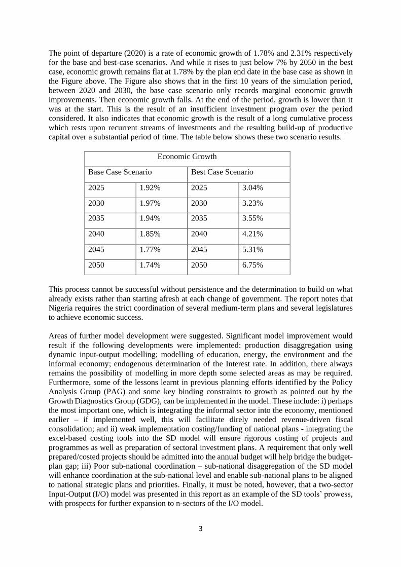
The point of departure (2020) is a rate of economic growth of 1.78% and 2.31% respectively
for the base and best-case scenarios. And while it rises to just below 7% by 2050 in the best
case, economic growth remains flat at 1.78% by the plan end date in the base case as shown in
the Figure above. The Figure also shows that in the first 10 years of the simulation period,
between 2020 and 2030, the base case scenario only records marginal economic growth
improvements. Then economic growth falls. At the end of the period, growth is lower than it
was at the start. This is the result of an insufficient investment program over the period
considered. It also indicates that economic growth is the result of a long cumulative process
which rests upon recurrent streams of investments and the resulting build-up of productive
capital over a substantial period of time. The table below shows these two scenario results.
Economic Growth
Base Case Scenario Best Case Scenario
2025 1.92% 2025 3.04%
2030 1.97% 2030 3.23%
2035 1.94% 2035 3.55%
2040 1.85% 2040 4.21%
2045 1.77% 2045 5.31%
2050 1.74% 2050 6.75%
This process cannot be successful without persistence and the determination to build on what
already exists rather than starting afresh at each change of government. The report notes that
Nigeria requires the strict coordination of several medium-term plans and several legislatures
to achieve economic success.
Areas of further model development were suggested. Significant model improvement would
result if the following developments were implemented: production disaggregation using
dynamic input-output modelling; modelling of education, energy, the environment and the
informal economy; endogenous determination of the Interest rate. In addition, there always
remains the possibility of modelling in more depth some selected areas as may be required.
Furthermore, some of the lessons learnt in previous planning efforts identified by the Policy
Analysis Group (PAG) and some key binding constraints to growth as pointed out by the
Growth Diagnostics Group (GDG), can be implemented in the model. These include: i) perhaps
the most important one, which is integrating the informal sector into the economy, mentioned
earlier – if implemented well, this will facilitate direly needed revenue-driven fiscal
consolidation; and ii) weak implementation costing/funding of national plans - integrating the
excel-based costing tools into the SD model will ensure rigorous costing of projects and
programmes as well as preparation of sectoral investment plans. A requirement that only well
prepared/costed projects should be admitted into the annual budget will help bridge the budget-
plan gap; iii) Poor sub-national coordination – sub-national disaggregation of the SD model
will enhance coordination at the sub-national level and enable sub-national plans to be aligned
to national strategic plans and priorities. Finally, it must be noted, however, that a two-sector
Input-Output (I/O) model was presented in this report as an example of the SD tools’ prowess,
with prospects for further expansion to n-sectors of the I/O model.

4
Table of Contents
EXECUTIVE SUMMARY ...................................................................................................... 1
CHAPTER 1: INTRODUCTION & BACKGROUND ................................................................... 6
a. Draft Final Report ..................................................................................................... 6
CHAPTER 2: REVIEW OF MACROECONOMIC DEVELOPMENTS IN NIGERIA........................... 7
a. Brief Overview of previous planning efforts ................................................................................................. 7
ii. Lessons learned from planning efforts of the last 20 years: ................................................................... 9
iii. Government Priorities, Global Megatrends and Growth Diagnostics .......................................................... 10
iv. Policy Implications: ....................................................................................................................................... 10
v. Policy recommendations on the basis of the GD analysis include the following: ........................................ 11
vi. Integration of key concepts and inputs from the Policy Analysis and the Growth Diagnostic Groups into the SD-based Model for Agenda 2050 Macro Framework: ................................................................................... 11
b. Macroeconomic developments in the last 20 years ................................................................................... 12
CHAPTER 3: APPROACH AND METHODOLOGY ................................................................. 14
a. Overview of approach, methods and tools: ................................................................................................ 14
b. Steps of System Dynamics Modelling. ........................................................................................................ 15
CHAPTER 4: SYSTEM DYNAMICS MODEL .......................................................................... 18
a. Key Concepts and Model Structures............................................................................................................ 18
b. The key feedback loops of the Nigerian socio-economy ............................................ 18
c. Model sketch, constants and parameters ................................................................. 25
d. Assumptions, Scenarios and Simulations .................................................................. 33
CHAPER 5: ANALYSIS OF PRELIMINARY RESULTS .............................................................. 34
Figure 25. Scenario comparison. Debt to GDP ratio.......................................................... 35
Figure 26. Population and national income ..................................................................... 36
Figure 27. Unemployment ............................................................................................... 37
Figure 28. National income per head ............................................................................... 38
Figure 29. Productive capital ........................................................................................... 39
Figure 30. Economic growth ............................................................................................ 40
Figure 32. Best scenario: economic growth...................................................................... 41
Figure 33. Government revenues & expenditures ............................................................ 41

5
Figure 34. Government surplus / deficit ........................................................................... 42
Figure 35. Government debts .......................................................................................... 43
Figure 36. Debt servicing................................................................................................. 44
Figure 37. International trade ......................................................................................... 45
Figure 38. Forex reserves ................................................................................................ 46
Figure 39. The naira exchange rate ................................................................................. 47
Figure 40. Extract from the data entry worksheet. Relationship forex stock – exchange rate ...................................................................................................................................... 48
Figure 41. The exchange rate multiplier .......................................................................... 49
CHAPTER 6: FURTHER MODEL DEVELOPMENT - DYNAMIC INPUT-OUTPUT MODEL .......... 49
Figure 42. System dynamics sketch of the orders – inventory causal connection ............... 50
Figure 43. Stock and production adjustment ................................................................... 50
Figure 44. Labour force dynamics .................................................................................... 51
Figure 45. Material input procurement ........................................................................... 51
Figure 46. Complete causal structure of a single sector .................................................... 52
APPENDIX 1: MODEL EQUATIONS ................................................................................... 52
APPENDIX 2: SOME BIBLIOGRAPHICAL REFERENCES ........................................................ 61

6
CHAPTER 1: INTRODUCTION & BACKGROUND a. Draft Final Report: This Draft Final Report is submitted by NSF Developments Ltd,
a development management, planning and training consultancy, based in Abuja, in respect
to the consultancy assignment by the Federal Ministry of Finance, Budget and National
Planning (FMFBNP) - to prepare a macroeconomic framework for Nigeria Agenda 2050
using the Computable General Equilibrium (CGE) model and the System Dynamics-based
Model referenced to the integrated Sustainable Development Goals (iSDG) model.
b. Background: Nigeria is in the process of developing successor plans to the Economic
Recovery and Growth Plan (ERGP, 2017-2020) and the Nigeria Vision 20: 2020, both of
which are ending by December 2020. Consequently, the Government of Nigeria has taken
steps to ensure the preparation of a Medium-Term National Development Plan (2021-
2025), or MTNDP to replace the ERGP (2017-2020) and a Long-Term National
Development Plan (LTNDP), the Nigeria Agenda 2050 Perspective Plan to take the place
of the Nigeria Vision 20:2020, using globally acceptable economic development and
planning models.
c. Planning Models: In order to accomplish this task, a number of models have been
identified for use by the supervising authority, the FMFBNP, for use in developing the
macroeconomic framework for the preparation of the two plans. Thus, for the MTNDP the
macro econometric model is to be used, together with the input-output model; while for the
LTNDP the Computable General Equilibrium (CGE) model is to be used in conjunction
with the system dynamics-based model derived with reference to the integrated Sustainable
Development Goals (iSDG) model. Modelling consultants were therefore engaged to
design, implement and train users of the four models in the Ministry, according to the Terms
of Reference.
d. Terms of Reference: The overall objective of the consultancy services is to develop a
dynamic CGE model and a system dynamics-based model of the Nigerian economy for use
by the FMFBNP in policy impact analysis. The output of the models would be used for the
preparation of the Macroeconomic Framework for the Perspective Plan called “Nigeria
Agenda 2050”. The two models are expected to be complementary in terms of operation
and consistency in the use of economic variables; while the output of one model may be
used as an input for the other model, the results of one may also be used to validate the
result of the other. Specific terms of reference include:
i. Review the existing DCGE/CGE models and iSDG model, with a view to presenting
options and solutions to problems in the Nigerian economy;
ii. Develop a theoretical and methodological framework for the DCGE and iSDG models
in Nigeria;
iii. Prepare a possible set of indicators for the models and determine their frequency,
accessibility and sources; and gather data on relevant indicators in excel format;
iv. Update a DCGE Model/SAM for Nigeria and iSDG Model that can be calibrated to
analyse the impact of changes in policy variables and/or economic shocks using
appropriate statistical software;
v. Provide in excel format the output of the model including draft forecasts and
assessment model simulation results
vi. Generate user manuals that contains the theoretical framework of the DCGE and iSDG
models, containing the equations, variables used to include their sources, and the
procedure for conducting simulations or sensitivity analysis, updating the parameter,
and error diagnostics, etc. and;

7
vii. Conduct consultative workshop among the technical staff of FMFBNP, CBN, DMO,
BOF, SEC, NNPC, DPR, NCS, OAGF, FIRS, NBS, NISER, NASS, PEAC and key
sectors to solicit comments suggestions to enhance the initial DCGE and iSDG models;
viii. Enhance capacity of FMFBNP technical staff in updating the DCGE and iSDG Models
for Nigeria and conducting policy analysis using the model through hands-on trainings
and exercises and ensure technological transfer in updating, re-estimating and
calibrating the model.
CHAPTER 2: REVIEW OF MACROECONOMIC DEVELOPMENTS IN NIGERIA a. Brief Overview of previous planning efforts
i. Historical Evolution
The historical evolution of previous planning efforts in Nigeria in the post-colonial era can
be categorized into three phases as described below:
a) The development planning phase (1962-1985). There were four National Development
Plans launched between 1962 and 1985. These were the plans for 1962-1968, 1970-1974,
1975-1980 and 1981-1985. Government intervention was dominant, coordination among
regions was lacking, with modest growth and macroeconomic imbalances.
b) The Structural Adjustment Programme (SAP) and policy-oriented planning era (1985-
1999). This phase was characterized by SAP (1985-1989) and 3-year Rolling Plans, 1990-
1992, 1993-1995, 1996-1999. With an International Financial Institutions led development
agenda, promoting private sector participation through deregulation, liberalization and
privatization, and macroeconomic stabilization leading to macro-economic imbalances and
mixed outcomes;
c) The high growth and development phase (2000-present): The return to development
planning witnessed ambitious home-grown initiatives, with high economic growth rates
but no job or social development gains.
Below is a schematic diagram of the historical evolution of previous planning efforts in
Nigeria.

8
Figure 2: Historical evolution of development planning-policy framework, institutional
configuration and outcomes – in Nigeria:
Source: Adapted from UN ECA (2016)
1.Development Planning 2.Government led interventions 3.Poor policy coordination
Development Outcomes
Macroeconomic and
Development Policy
Framework
Institutional Configuration
1.Modest economic growth rates 2. Structural change -some sectoral shifts 3. Macro imbalances developed over time
1.Little coalition between government and private agents 2.Government-dominant in command but week in capacity 3. Private agents-weak
1.Policy-oriented Planning 2.Liberalisation-deraegulation-privatisation 3. Macroeconomic stability
1.Lower or negative per capital growth 2. Productivity-reducing structural change 3. Macro imbalances developed over time
1.Aid donors dominated 2. Little coalition between government and private agents 3.Government-weak and dwindling resources 3.Private agents-disfranchised and fragmented
1.Home grown development
initiatives 2.Return to development planning 3.Ambitious goals
1.High economic growth rates 2.Growth didn’t trigger structural transformation despite stronger planning 3.Social development gains were achieved but not at a scale
1.Renewed faith in development planning, better policy formulation/implementation and better fiscal/monetary management
Development Planning phase,
1962-1985
Structural Adjustment
Programme, Policy oriented planning
1985-1999
High Growth & Development Phase,
2000-Present

9
ii. Lessons learned from planning efforts of the last 20 years: A few of the Plans reviewed by the Policy Analysis Group (PAG) over the last 20 years include:
• The National Economic Empowerment and Development Strategy (NEEDS), which built
on the Interim Poverty Reduction Strategy Paper (IPRSP) between 2001 and 2003, and
incorporated the State Economic Empowerment and Development Strategies (SEEDS) and
Local Economic Empowerment and Development Strategies (LEEDS)
• Nigeria Vision 20:2020 (NV 20:2020) and the 1st medium-term national implementation
plans (NIPs)
• The Transformation Agenda (2011 – 2015)
• The Economic Recovery and Growth Plan (ERGP, 2017-2020)
Upon analyzing these various strategic documents that have guided Nigeria’s national
development policy over the past 20 years and even before, the group has deducted and
recommended that the country should avoid potential pitfalls both in the planning phase and
the implementation stage that have characterized national planning in the past. Table 1 below
exhibits some of the lessons learned from implementation of previous National Development
Plans in Nigeria.
Table 1: Lessons learned from previous National Development Plans
Weak link between
the plan and annual
budget
Key components of development plans are skipped or provided with less fund during
the preparation of the government annual budget.
Less emphasis on
inter-sectors
collaboration
There is little focus on building inter sectoral synergies for economic development.
Heavy reliance on
foreign funding
Relying on foreign funding is a major throwback for the implementation of several
plans. Most plans were also silent on implementation cost/funding.
Absence of
coordinating
institution(s) for
plan
implementation
This resulted in limited implementation capacities as well as issues of continuity and
coordination of programmes.
Less on addressing
key domestic
growth constraints
Several of the development plans skipped addressing key domestic growth and
productivity constraints. As a result, these issues became huge impediments to the
attainment of set targets.
Impact of oil prices Fluctuations in oil prices can have negative impact on Nigeria’s foreign exchange and
government revenue earnings culminating in severe macroeconomic shocks and
instability
Effect of political
changes
Plan implementation often affected by political and policy changes
Public vs private
investment
Public investment was promoted at the expense of private investment
Internal and
external pressures
Government often failed to keep scheduling and targets because of internal and external
pressures

10
iii. Government Priorities, Global Megatrends and Growth Diagnostics The simulations of the SD model are informed by findings of other sub-groups that
analyzed and reviewed previous plans, government priorities, megatrends in the global
economy and growth diagnostics. Presidential Priorities consist of the following objectives:
Stabilization of the economy
Achieving Agricultural and Food Security
Ensuring Energy Sufficiency in Power and Petroleum Products
Improving Transportation and Other Infrastructures
Driving Industrialization
Improving Health, Education, and Productivity of Nigerians
Enhancing Social Security and Reducing Poverty
Fighting Corruption and Improving Governance, and
Improving Security for all Citizens.
A few of the mega trends that will be expected to affect the planning process in Nigeria
include:
Economic Globalization: e.g., gradual shift in the global economic power relations
from the current industrialized countries to the rising and emerging markets;
increasingly connected global economy and economic integration…
Technology and the Digital Revolution: e.g., Artificial intelligence; 4th Industrial
Revolution (Industry 4.0); Internet of Things…
Demographics and Mobility: e.g., Hyper-urbanization; Rise of the middle class in
Asia and Africa; Demographic dividend…
Energy and Environment: e.g., Resource Constraints, Climate Change; Changing
Energy Mix…
Innovation Acceleration: e.g., Knowledge and Information Society…
Health and Wellness: Involving consumption; Demand for better health care
Global Security Risks: e.g., Pandemics; Natural Catastrophe; Cyber Attacks;
Terrorism…
iv. Policy Implications: The policy recommendations of the Policy analysis Group and Growth Diagnostics Group
are as follow:
• In budgetary provisions, the proportion of capital expenditure should be increased,
and implementation of capital budgets should be scaled up.
• The cost of governance should be reduced by at least 30%.
• Emphasizing movement away from dependence on crude oil
• Closing the fiscal gap to about 3% of GDP
• Stimulating the economy and business development
• Increasing post COVID-19 investment to 9% of GDP
• Diversifying the product space – whether agricultural or non-agricultural products,
particularly products that could earn foreign exchange for the country other than the
oil sector
• Adopt transformative trade policies
• Prioritize self-reliance and home-grown solutions, including import-substitution
• Reduce post-harvest losses in agriculture to stabilize prices
• Measures to diversify revenue and increase tax to GDP ratio by improving tax
administration, including the informal sector and widening the tax base.
• Enhance non-oil forex earnings by attracting FDI, improving diaspora remittances
and promoting non-oil exports.

11
• Prioritization and implementation of critical and strategic infrastructure projects
that will directly boost production and productivity in the SME, agriculture,
manufacturing and service sectors, in line with rapid growth, revenue and forex
diversification objectives.
v. Policy recommendations on the basis of the GD analysis include the following: Minimize macroeconomic volatility by strengthening domestic financial
institutions
Improve access to finance and credit to the private sector by removing existing
regulatory impediments
Strengthen legal and judicial reforms commensurate with economic reforms so as
to establish a stable policy environment in order to boost private investments
Ensure sufficient energy provision, particularly electricity, to enhance private
production
Focus policy on microfinance banking activities, which remain too minimal in
Nigeria and at times even financed by foreign firms, including improving access to
funding and intermediation.
vi. Integration of key concepts and inputs from the Policy Analysis and the Growth Diagnostic Groups into the SD-based Model for Agenda 2050 Macro Framework:
The SD-based Model for Agenda 2050 has the capability to incorporate many of the
lessons learnt from previous planning efforts and the recommendations of the other
Groups – PAG and GDG, a few examples of which include the following, some of which
have already been implemented in the model:
• Relaxing some of the growth constraints identified by the GDG – Feedback loops
in the SD model identify the leverage points where policy action can bring about
the desired development outcomes and impacts.
• Addressing the weak budget-plan link and poor implementation costing/funding of
projects and programmes – the SD model can incorporate the excel-based costing
tools to enable policy analysts in the MFBNP and line Ministries prepare investment
plans and detailed costing of interventions that can be used in programming
expenditures in the budget.
• To address diversification of revenue sources, increase the tax/GDP ratio, integrate
the informal sector and widen the tax base using the SD-based modelling approach.
• Strengthening the Sub-national coordination function of the MFBNP – By carrying
out the sub-national disaggregation of the analysis at the national level using the SD
Model the MFBNP will have a strong tool to deploy in the coordination of planning
at the sub-national level.
• The recommendation that government consumption (recurrent costs in the budget)
should be reduced by 30% while government investment (capital expenditure in the
budget) be increased has already been implemented in the SD Model for Agenda
2050.
• To facilitate the seamless integration of some of the many planning models/tools
and ensure complementarity for medium- and long-term planning, we have done an
SD version of a simple input/output model for demonstration to the Ministry. This
basic SD version of the I/O Model can be developed further if required.

12
b. Macroeconomic developments in the last 20 years In May 1999, after nearly two decades of military dictatorship, Nigeria ushered in a new
administration. The new government’s target was to accelerate economic growth to alleviate
Nigeria’s widespread poverty. In year 2000, the proportion of Nigerians living below the
poverty line of one dollar a day was 56 per cent. This proportion had increased dramatically
during the preceding two decades.
But growing poverty is not the only challenge Nigeria has been facing in the last 20 years. A
fast-growing population, mounting unemployment, particularly youth unemployment,
persistent corruption, a continued heavy reliance on hydrocarbons and the heavy cost of
governance are serious additional difficulties.
Viewed as a global socio-economy, Nigeria was not making significant progress. In 2000,
both per capita income and per capita private consumption were lower than in the early 1970s.
The first decade of the 21st century confirmed the strong influence of oil price variations on
Nigeria’s growth performance. Between 2000 and 2014, Nigeria’s GDP grew at an average
rate of 7% per year. An annual rate of 7.3% was even reached in 2011/12. But growth did
not translate into a strong diversified economy. Oil, gas, and agricultural output continued to
dominate wealth generation, contributing around 70% of total output. Oil alone accounted
for more than a third of GDP. Oil had risen from 58% of exports in 1970 to more than 90%
in the 2000s. It is during this period that Nigeria discovered a new economic evil: non-
inclusive growth.
In 2010, extreme poverty, the share of population living on less than $1.25 a day, not only
persisted but significantly increased to about 68% of the population in 2010. More recently,
the instability in the North and the resulting displacement of people have contributed to the
high incidence of poverty in the North East.
Following the oil price collapse in 2014-2016, combined with negative production shocks,
Nigeria’s GDP growth dropped to 2.7% in 2015. In 2016 during its first recession in 25 years,
the economy contracted by 1.6%. Domestic demand remained constrained by stagnating
private consumption in the context of high inflation: 11% in the first half of 2019. On the
production side, growth in 2019 was primarily driven by services, particularly telecoms.
Agricultural growth remained below potential due to continued insurgency in the Northeast
and ongoing farmer-herdsmen conflicts. Industrial performance was mixed. Oil GDP growth
was stable, while manufacturing production slowed down in 2019 due to a weaker power
sector performance. Food and beverages output increased in response to import restrictions.
Construction continued to perform positively, supported by ongoing megaprojects, higher
public investment and import restrictions.
The Nigerian economy does not grow fast enough, and the Nigerian population grows too
fast to lift the bottom half of the population out of poverty. Prospects for the rural poor are
grim due to the weakness of the agriculture sector, and the livelihoods of the urban poor are
adversely affected by high food prices.
Employment is another major concern. Formal employment is low while Nigeria’s informal
sector accounts for between 65% and 70% of total employment. Rising unemployment has
become a permanent feature of the Nigerian economy: 4% in 1986, 13% in 2007 and 23-25%
in 2018 with another 20% of the labour force underemployed. Youth unemployment is an
even bigger challenge estimated at 38-40% in the last years of the 2010s. Nigeria’s

13
employment problem is a simple arithmetic operation: employment creation remains
insufficient to absorb a much faster growing labour force.
Today, Nigeria’s external reserves stand at US$37 billion. External reserves rose from $4
billion in 1999 to $46 billion in 2010 after paying $12 billion in 2005 to liquidate the external
debt. The highest level of foreign reserves was observed in 2007/8 with a stock reaching
US$52/54 billion. Worth noting, it is also in the period 2006/8 that the naira exchange rate
appreciated. An empirical observation which gives some validity to our model structure. The
naira exchange rate passed the 100 mark for the first time in 2000 with ₦102 per US$. It then
increased to ₦306 per US$ in 2018. Today, the official rate is ₦380 for an American dollar
but the parallel market trades US dollar at ₦470.
Nigeria’s overall global competitiveness remains weak. This is due to the quantity and quality
of health, primary education and infrastructure.
One of Nigeria’s core strategies is a public-private partnership in investments, especially in
such core infrastructure projects as power, railways, roads and ports to generate employment
opportunities. But the private sector in general remains relatively weak. A large part of it is
the oil economy which has been unable to create linkages to the rest of the economy to
significantly contribute to structural change and transformation.
Nigeria is faced with problems both in implementation and in choice. It is not the right
approach to try and fix all problems simultaneously. It spreads thin resources too thin and
does not achieve much. One of the first lessons that economics students learn is that an
economy is a highly connected dynamic system. As a result of economic linkages, fixing one
important problem may result in fixing a number of others. It may also result in creating new
challenges.
Even with significant structural policy reforms, and considering climate change, the likely
fate of the international oil market and the likely appearance of Covid-type new challenges,
it will take a long time for Nigeria’s economic growth to go back to the performance of ten
years ago. For some time, the economy might even grow more slowly than the population,
leading to worsening living standards. Among the many factors that constrain economic
growth, rising public debt, inflation, multiple exchange rate windows and subsidies play a
role. But perhaps the most important is the lack of revenue-driven fiscal consolidation.
Nigeria is faced with the huge task of institutionalizing a large informal economy which
operates on a day to day basis outside of any formal financial and economic structures.
Another major challenge is to support the sustained growth of the non-oil economy. Reforms
in this direction would help raise living standards of low-income groups, reduce the size of
the informal economy and create job opportunities. It is indeed the lack of job opportunities
which is at the core of the high poverty levels, of regional inequality, and of social and
political unrest in the country.

14
CHAPTER 3: APPROACH AND METHODOLOGY a. Overview of approach, methods and tools: System dynamics is one of the
approaches selected to develop a macro framework for Nigeria Agenda 2050. System
Dynamics is the brainchild of late Professor Jay W. Forrester of the Massachusetts
Institute of Technology (MIT). System Dynamics is neither a theory nor a solution. It
is a method, that is, a vision of how the world works and it is a tool, that is, a means to
an end.
System dynamics rests on four foundations:
• The theory of information feedback systems;
• A knowledge of decision‐making processes;
• The experimental model approach to complex systems;
• The digital computer as a means to simulate realistic mathematical models.
The purpose of system dynamics practitioners is to build models capable of deriving
dynamic behaviours solely from variables and interactions belonging to and within the
system. The dynamics of systems does not depend upon any exogenous forces but is
endogenously generated by their structure.
System dynamics models are built on four pillars:
• Stocks & flows
• Feedback loops
• Non-linearity
• Time & delays
i. Stocks and flows are key system dynamics variables. Stocks are accumulators. Flows
feed and/or drain stocks. Examples of stocks and flows abound. Population is a stock
fed by births and drained by deaths; your bank account is a stock fed by your deposits
and drained by your withdrawals; a trader’s inventory is a stock fed by goods
produced and drained by goods shipped; your reputation is a stock fed by all the good
things you do and drained by all the bad things you accomplish; a price is a stock fed
by inflation and drained by deflation.
ii. Feedback loops are closed chains of multiple, causal interconnections linking stocks
and flows. They also often include time delays and non-linear interactions. It is the
interplay of these loops which determines system’s behaviour. Feedback loops are
major structural elements in system dynamics models. They are of two types:
reinforcing and balancing. Reinforcing loops generate exponential growth or
exponential decline. These are popularly known as virtuous and vicious circles. If
unchecked reinforcing loops explode or collapse leading to unmanageable situations.
In contrast, balancing loops counteract system growth or system decline. They thrive
to create equilibrium, that is, system stability. One of the favourite examples cited by
system dynamics textbooks is the dynamics of population. Population is a stock
driven by two major flows: births and deaths which both depend on population size.
But births and deaths also affect population size. There exists therefore a dynamic
system driven by two feedback loops of opposing polarity. The interactions between
births and population create a reinforcing loop which feeds upon itself. The
interactions between deaths and population create a balancing loop which counteracts
the effect of births and thrives to balance the system. For economists, the virtue is in
reinforcing loops because economic growth remains the gospel of the profession. For
physicists and natural scientists, however, the virtue is in balancing loops because

15
equilibrium means system stability. This fundamental difference of perspective
explains why it is so difficult to reach a compromise between economic growth and
the preservation of nature.
iii. Non-linearity is a characteristic of many natural and made-made systems. It is a
reaction to stimulus in a manner non-proportional to the action that caused the
response. System dynamics models do incorporate non-linear relationships either as
equations or as user-defined functional tables. Examples of functional tables include
a multiplier of importation which is assumed to be influenced by the exchange rate
or the effect of the income per head on the population’s fertility. These assumed
functional relationships may be modified but the direction of the effect (direct or
inverse) should be preserved. For example, fertility is supposed to decrease and not
increase when the economy creates more wealth.
iv. Time is the most important variable in a system dynamics model. It is time together
with the stocks included in the model which generate its dynamics. This is because
the future value of each stock partly depends upon its present value:
STOCKT+TIME STEP = STOCKT + TIME STEP * (FLOW INT – FLOW OUTT)
In the above equation, T is the index of current time and TIME STEP is the Δ time
also known as DT. TIME STEP is a parameter of the integration process driving its
accuracy. It is not a parameter of the model. System dynamics models most
frequently use Euler as their integration method. Flows are calculated from values of
stocks, other flows and/or from auxiliary variables. Auxiliary variables are
components of flows. They are made explicit to clarify how complex flows are
calculated.
v. Delays: very few relationships, if any, are instantaneous. System dynamics include a
number of delay functions to take account of this reality. Delays are fixed or
exponential, material or information, and of order 1, 3 or n.
It is our conviction that system dynamics is the right perspective to address the
dynamic complexity of such large adaptive systems as states, regions or whole
countries. System dynamics is a valuable approach for high level issues such as
corporate strategy and government policy. It is and has been widely used to look at a
variety of issues such as industry structure, urban dynamics, population, public health,
engineering prototyping, risk assessment and such global concerns as economic
development and environmental protection.
b. Steps of System Dynamics Modelling. Not every system dynamics model constructed
is substantial. But when it is there should be six steps in its construction. Interestingly
enough these six steps are in a feedback loop:
• Conceptualization – group model building
• Sketch
• Identification of feedback loops
• Equations & units
• Simulations & calibration
• Back to sketch or perhaps even to conceptualization for potential model
improvement

16
i. Conceptualization. The first step in system dynamics modelling is group model
building to get the concept right and accepted by all. Models built with system
dynamics address a large variety of issues. But system dynamics modelers cannot
be experts in all the fields they model especially when multidisciplinarity is a key
model requirement. The corollary of such an approach is that such models, which
call for multidisciplinarity, are never build by one person. If they were, they would
fail. The specific skill of system dynamics modelers is to capture experts’ expertise
– to extract experts’ mental model and to transform it into a formalized and explicit
computable structure which exploits this expertise to uncover interventions and
policy decisions favorable to the system under study. Much if not all of the
knowledge and information required to build a substantial system dynamics model
reside in the mental models of those that are part of the system under study.
Participating in model construction also enhances the learning process of those to
whom the model is destined. Modelling a problem always results in considerable
learning for those participating in the modelling process. Finally, model validity
and model implementation - the trust model recipients put on the model greatly
benefit from group model building. Even the most brilliantly built model includes
debatable structures and debatable assumptions. Multidisciplinarity is therefore not
the only requirement. It is also required to reconcile different visions of the same
problem to reach consensus on how to solve a problem or to reach a goal. This is
certainly the case for a model of the very long term such as the present macro
framework model. To some extent, the approach adopted by Government in the
preparation of Nigeria Agenda 2050 resembles group model building although
there is room for perfecting it.
ii. Sketch. System dynamics model are built graphically on a workbench called view.
As an example, the equation presented in 3a under non-linearity is represented by
the following sketch:
Figure 1. Stock & flow sketch in system dynamics
Stocks are balance sheet elements with no time dimension which accumulate money,
material, people or information. The double arrows represent the movement of stuff in
and out of the stock. Causality, which is not correlation, is represented by a single arrow
starting from the cause and pointing to the effect.
STOCKFlow in Flow out
Initial stock
17
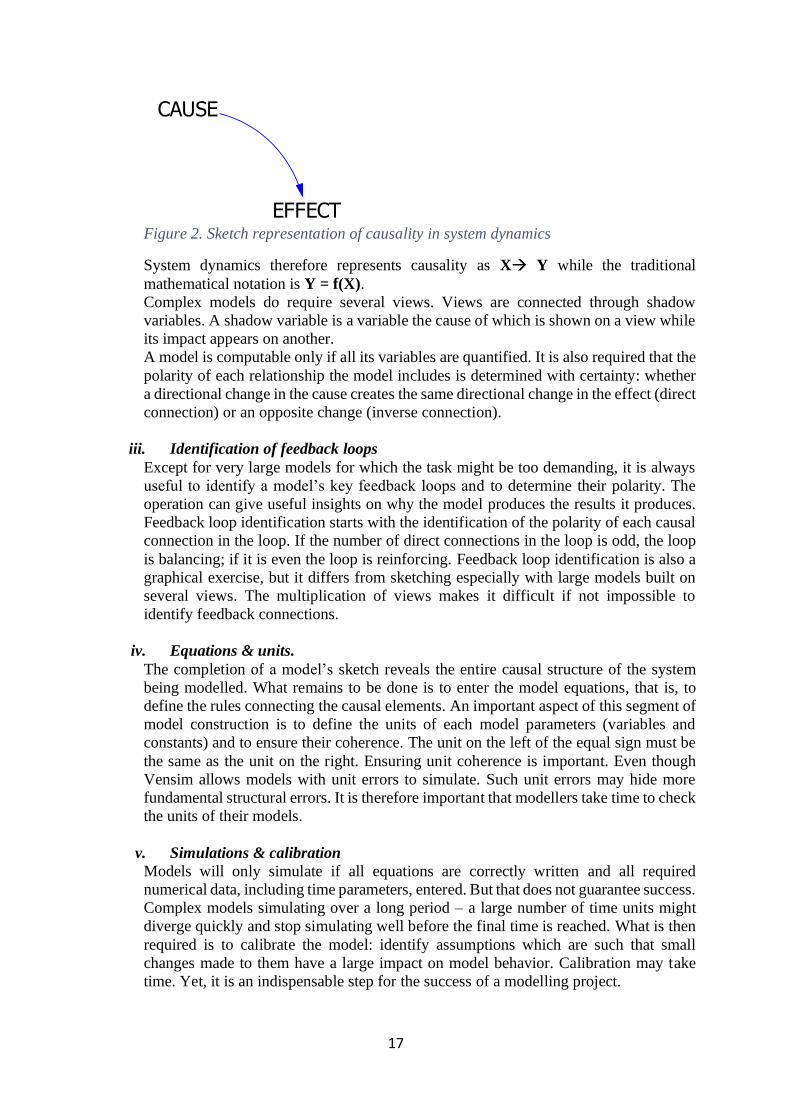
Figure 2. Sketch representation of causality in system dynamics
System dynamics therefore represents causality as X Y while the traditional
mathematical notation is Y = f(X).
Complex models do require several views. Views are connected through shadow
variables. A shadow variable is a variable the cause of which is shown on a view while
its impact appears on another.
A model is computable only if all its variables are quantified. It is also required that the
polarity of each relationship the model includes is determined with certainty: whether
a directional change in the cause creates the same directional change in the effect (direct
connection) or an opposite change (inverse connection).
iii. Identification of feedback loops
Except for very large models for which the task might be too demanding, it is always
useful to identify a model’s key feedback loops and to determine their polarity. The
operation can give useful insights on why the model produces the results it produces.
Feedback loop identification starts with the identification of the polarity of each causal
connection in the loop. If the number of direct connections in the loop is odd, the loop
is balancing; if it is even the loop is reinforcing. Feedback loop identification is also a
graphical exercise, but it differs from sketching especially with large models built on
several views. The multiplication of views makes it difficult if not impossible to
identify feedback connections.
iv. Equations & units.
The completion of a model’s sketch reveals the entire causal structure of the system
being modelled. What remains to be done is to enter the model equations, that is, to
define the rules connecting the causal elements. An important aspect of this segment of
model construction is to define the units of each model parameters (variables and
constants) and to ensure their coherence. The unit on the left of the equal sign must be
the same as the unit on the right. Ensuring unit coherence is important. Even though
Vensim allows models with unit errors to simulate. Such unit errors may hide more
fundamental structural errors. It is therefore important that modellers take time to check
the units of their models.
v. Simulations & calibration
Models will only simulate if all equations are correctly written and all required
numerical data, including time parameters, entered. But that does not guarantee success.
Complex models simulating over a long period – a large number of time units might
diverge quickly and stop simulating well before the final time is reached. What is then
required is to calibrate the model: identify assumptions which are such that small
changes made to them have a large impact on model behavior. Calibration may take
time. Yet, it is an indispensable step for the success of a modelling project.
CAUSE
EFFECT

18
A set of numerical data that leads to a successful simulation is a scenario. System
dynamics models can produce a large number of scenarios in a very short time. It is
important to change one assumption at a time and to take time to understand why the
model produces the results it produces.
vi. Back to sketch
It may happen that simulation results produce inconsistencies or impossibilities or
reveal structural deficiencies or point to missing structures in the model or that any
combination of the above is observed. It is then necessary to rethink the concept and to
go back to the design of the model. Complex models are better built on a step by step
basis so that complexity is always under control. The building of system dynamics
models is therefore a feedback loop.
CHAPTER 4: SYSTEM DYNAMICS MODEL a. Key Concepts and Model Structures
In its present state, which we do not consider as the final state, the model depicts the
interactions of two major social structures: population and the global economy. The
economy is not disaggregated, and the environment is not modelled. Those are two
critical and required additions. It would not pose any major problem to disaggregate the
economy and build the environment in the model. It might even be useful to review the
existing model structure with the purpose of improving it. For this to be done, more time,
additional expertise and the implementation of group model building are required.
b. The key feedback loops of the Nigerian socio-economy are represented
in 11 diagrams. The diagram on Figure 3 shows the four reinforcing loops which drive
population growth through fertility rate and income per head. The sketch also shows a
potential connection between the economy and the population that would be created if a
policy existed to link investment volumes to the level of unemployment. This causal link,
however, has not been built in the model as it is not the purpose of models to substitute
for decision makers.
Figure 3. Population and the economy
VERY YOUNG(0-4)
Yearly births
SCHOOLAGE (5-14)
Growing toschool age
YOUNG ADULT(15-24)
ADULT(25-64)
Maturing toyoung adult Maturing to
adult
Laboursupply to
theeconomy
Unemployment
Labour requiredby the economy
PRODUCTIVECAPITAL
Fertilityrate
Indicated impact ofincome per head on
fertility rate
Income perhead index
Populationtotal
Income perhead
GDPfc
GDPmp
Nationalincome Investment
LINKAGES POPULATION - ECONOMY
Labouravailable
R
R
R
R
B
B

19
The two loops that would be created if the model had built in a formal policy to link investment
to unemployment are both balancing. This is because an increase (decrease) in the labour force
that population supplies to the economy creates more (less) investment and a higher (lower)
GDP which tends to reduce (increase) the fertility rate.
Evidently, this relationship is not instantaneous. The reaction of the population to the stimulus
generated by changes in the income per head is assumed to occur continuously and
progressively over a period of 5 years. This is indicated by a constant called delay impacting
on fertility.
Figure 4 displays the model’s major causal connections. Although this model is relatively
simple – with the exclusion of the population segment it has only five interconnected
differential equations, it is clear that this structure already constitutes a rather complex system
which only a computer can process. Understanding it requires further clarifying. This is the
purpose of the next nine diagrams.
Figure 4. Model major causal structures
The capital accumulation loop shown on Figure 5 represents the core of the economic growth
process. Each period, a proportion of the wealth created is reinvested in the stock of capital
which increases and produces more wealth. It is clearly a reinforcing process that feeds upon
itself.
Deficitfinancingdomestic
PUBLICDOMESTIC
DEBT
Interest paid ondomestic debt
Debtservicingdomestic
Debtservicing
total
Governmentexpenditures
Governmentsurplus/deficit
Governmentdomesticrevenues
Governmenttax revenue
Governmentnon-tax revenue
GDPfc index GDPfcPRODUCTIVE
CAPITAL
InvestmentGovernmentinvestment
Privateinvestment
Savings
Disposableincome
Nationalincome
GDPmp
Deficitfinancingforeign
PUBLICFOREIGN
DEBT
Interest paid onforeign debt
Debtservicingforeign
Productivecapital index
Capitalmultiplier of
non-oil export
Non-oilexport
Export
FOREIGNRESERVES
Desiredexchange
rateRATE OF
EXCHANGE
Forex in
Exchangerateindex
Forex out
Import
Exchangerate
multiplierof import
Exchange ratemultiplier of
non-oil export

20
Figure 5. The reinforcing capital accumulation loop
Two parameters are important here: the propensity to consume and the depreciation fraction of
the capital stock. The model also includes a third parameter called investment effectiveness. It
is a simple multiplier varying between 0 and 1. Lowering the value of investment effectiveness
is equivalent to assuming an imperfect flow of domestic saving to capital which may reflect
either capital flight or corruption or both. This parameter was not activated. It was kept neutral
(with the value 1) in the model simulations presented in this report.
By nature, a reinforcing loop is unstable and tends to make systems unmanageable except if
one or several balancing loops mitigate the exploding exponential growth or decay. One of
these loops is shown on Figure 6.
Figure 6. The first balancing tax loop
The income tax loop shows the stabilizing impact of taxation on the economy. More (less) tax
reduces (increases) disposable income, saving, investment and the stock of capital and
Deficit financingdomestic
PUBLICDOMESTIC DEBT
Interest paid ondomestic debt
Debt servicingdomestic
Debt servicingtotal
Governmentexpenditures
Governmentsurplus/deficit
Governmentdomestic revenues
Government taxrevenue
Governmentnon-tax revenue
GDPfc index GDPfcPRODUCTIVE
CAPITAL
InvestmentGovernmentinvestment
Privateinvestment
Savings
Disposableincome
Nationalincome
GDPmp
Deficit financingforeign
PUBLICFOREIGN DEBT
Interest paid onforeign debt
Debt servicingforeign
Productivecapital index
Capital multiplier ofnon-oil export
Non-oilexport
Export
FOREIGNRESERVES
Desiredexchange rate
RATE OFEXCHANGE
Forex in
Exchange rateindex
Forex out
Import
Exchange ratemultiplier of import
Exchange ratemultiplier of non-oil
export
R
Deficitfinancingdomestic
PUBLICDOMESTIC
DEBT
Interest paid ondomestic debt
Debtservicingdomestic
Debtservicing
total
Governmentexpenditures
Governmentsurplus/deficit
Governmentdomesticrevenues
Governmenttax revenue
Governmentnon-tax revenue
GDPfc index GDPfcPRODUCTIVE
CAPITAL
InvestmentGovernmentinvestment
Privateinvestment
Savings
Disposableincome
Nationalincome
GDPmp
Deficitfinancingforeign
PUBLICFOREIGN
DEBT
Interest paid onforeign debt
Debtservicingforeign
Productivecapital index
Capitalmultiplier of
non-oil export
Non-oilexport
Export
FOREIGNRESERVES
Desiredexchange
rateRATE OF
EXCHANGE
Forex in
Exchangerateindex
Forex out
Import
Exchangerate
multiplierof import
Exchange ratemultiplier of
non-oil export
B

21
dynamically results in less (more) tax revenue. While a reinforcing loop is such that an increase
(or a decrease) in any of its variables results in more increase (or decrease) in that same
variable, a balancing loop is such that an increase (or a decrease) in any of its variables results
in a decrease (or an increase) in that same variable. Applying this reasoning to taxation
demonstrates that it may end up being a good policy to reduce taxes to ultimately increase tax
revenue.
Figure 7 shows the two reinforcing government investment loops. Just like the private sector,
government uses part of its revenue to invest and contribute to the growth of the economy.
Both this structure and that shown on Figure 5 combine to produce the growth of the entire
economic system as they both aim at increasing the country’s stock of productive capital and
therefore GDP.
Figure 7. Two reinforcing government investment loops
The critical parameters in these feedback loops are the government propensity to consume and
invest. A high cost of governance may not necessarily reduce the contribution of government
to the country’s investment and growth but, if government does not run a budget surplus, it will
create more indebtedness and higher debt servicing obligations.
The model is constructed in such a way that no constraint is placed either on the size of deficit
financing, on public debts or on debt servicing both at home and abroad. Figure 8 displays the
reinforcing domestic debt loop and the deficit financing process as far as public domestic debt
is concerned.
Deficitfinancingdomestic
PUBLICDOMESTIC
DEBT
Interest paid ondomestic debt
Debtservicingdomestic
Debtservicing
total
Governmentexpenditures
Governmentsurplus/deficit
Governmentdomesticrevenues
Governmenttax revenue
Governmentnon-tax revenue
GDPfc index GDPfcPRODUCTIVE
CAPITAL
InvestmentGovernmentinvestment
Privateinvestment
Savings
Disposableincome
Nationalincome
GDPmp
Deficitfinancingforeign
PUBLICFOREIGN
DEBT
Interest paid onforeign debt
Debtservicingforeign
Productivecapital index
Capitalmultiplier of
non-oil export
Non-oilexport
Export
FOREIGNRESERVES
Desiredexchange
rateRATE OF
EXCHANGE
Forex in
Exchangerateindex
Forex out
Import
Exchangerate
multiplierof import
Exchange ratemultiplier of
non-oil export
R
R
22
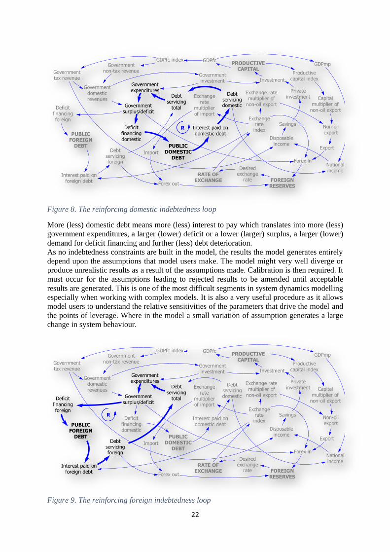
Figure 8. The reinforcing domestic indebtedness loop
More (less) domestic debt means more (less) interest to pay which translates into more (less)
government expenditures, a larger (lower) deficit or a lower (larger) surplus, a larger (lower)
demand for deficit financing and further (less) debt deterioration.
As no indebtedness constraints are built in the model, the results the model generates entirely
depend upon the assumptions that model users make. The model might very well diverge or
produce unrealistic results as a result of the assumptions made. Calibration is then required. It
must occur for the assumptions leading to rejected results to be amended until acceptable
results are generated. This is one of the most difficult segments in system dynamics modelling
especially when working with complex models. It is also a very useful procedure as it allows
model users to understand the relative sensitivities of the parameters that drive the model and
the points of leverage. Where in the model a small variation of assumption generates a large
change in system behaviour.
Figure 9. The reinforcing foreign indebtedness loop
Deficitfinancingdomestic
PUBLICDOMESTIC
DEBT
Interest paid ondomestic debt
Debtservicingdomestic
Debtservicing
total
Governmentexpenditures
Governmentsurplus/deficit
Governmentdomesticrevenues
Governmenttax revenue
Governmentnon-tax revenue
GDPfc index GDPfcPRODUCTIVE
CAPITAL
InvestmentGovernmentinvestment
Privateinvestment
Savings
Disposableincome
Nationalincome
GDPmp
Deficitfinancingforeign
PUBLICFOREIGN
DEBT
Interest paid onforeign debt
Debtservicingforeign
Productivecapital index
Capitalmultiplier of
non-oil export
Non-oilexport
Export
FOREIGNRESERVES
Desiredexchange
rateRATE OF
EXCHANGE
Forex in
Exchangerateindex
Forex out
Import
Exchangerate
multiplierof import
Exchange ratemultiplier of
non-oil export
R
23
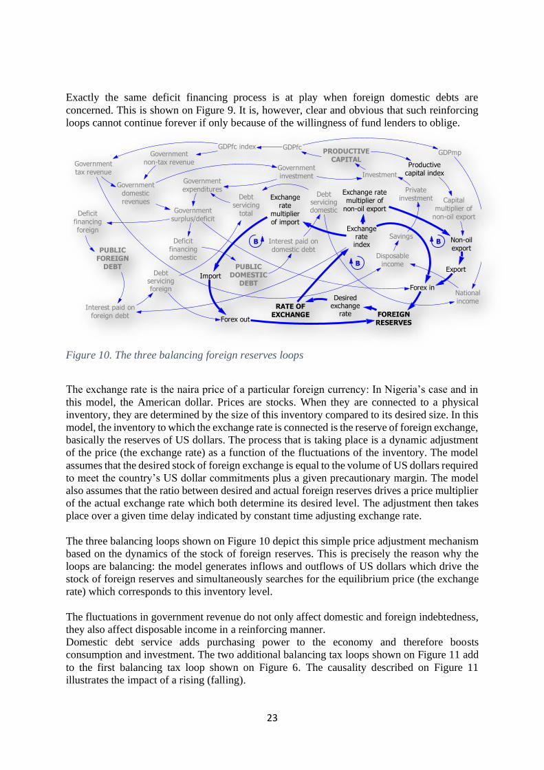
Exactly the same deficit financing process is at play when foreign domestic debts are
concerned. This is shown on Figure 9. It is, however, clear and obvious that such reinforcing
loops cannot continue forever if only because of the willingness of fund lenders to oblige.
Figure 10. The three balancing foreign reserves loops
The exchange rate is the naira price of a particular foreign currency: In Nigeria’s case and in
this model, the American dollar. Prices are stocks. When they are connected to a physical
inventory, they are determined by the size of this inventory compared to its desired size. In this
model, the inventory to which the exchange rate is connected is the reserve of foreign exchange,
basically the reserves of US dollars. The process that is taking place is a dynamic adjustment
of the price (the exchange rate) as a function of the fluctuations of the inventory. The model
assumes that the desired stock of foreign exchange is equal to the volume of US dollars required
to meet the country’s US dollar commitments plus a given precautionary margin. The model
also assumes that the ratio between desired and actual foreign reserves drives a price multiplier
of the actual exchange rate which both determine its desired level. The adjustment then takes
place over a given time delay indicated by constant time adjusting exchange rate.
The three balancing loops shown on Figure 10 depict this simple price adjustment mechanism
based on the dynamics of the stock of foreign reserves. This is precisely the reason why the
loops are balancing: the model generates inflows and outflows of US dollars which drive the
stock of foreign reserves and simultaneously searches for the equilibrium price (the exchange
rate) which corresponds to this inventory level.
The fluctuations in government revenue do not only affect domestic and foreign indebtedness,
they also affect disposable income in a reinforcing manner.
Domestic debt service adds purchasing power to the economy and therefore boosts
consumption and investment. The two additional balancing tax loops shown on Figure 11 add
to the first balancing tax loop shown on Figure 6. The causality described on Figure 11
illustrates the impact of a rising (falling).
Deficitfinancingdomestic
PUBLICDOMESTIC
DEBT
Interest paid ondomestic debt
Debtservicingdomestic
Debtservicing
total
Governmentexpenditures
Governmentsurplus/deficit
Governmentdomesticrevenues
Governmenttax revenue
Governmentnon-tax revenue
GDPfc index GDPfcPRODUCTIVE
CAPITAL
InvestmentGovernmentinvestment
Privateinvestment
Savings
Disposableincome
Nationalincome
GDPmp
Deficitfinancingforeign
PUBLICFOREIGN
DEBT
Interest paid onforeign debt
Debtservicingforeign
Productivecapital index
Capitalmultiplier of
non-oil export
Non-oilexport
Export
FOREIGNRESERVES
Desiredexchange
rateRATE OF
EXCHANGE
Forex in
Exchangerateindex
Forex out
Import
Exchangerate
multiplierof import
Exchange ratemultiplier of
non-oil export
BB
B

24
Domestic debt on national and disposable income through debt servicing. More (less)
disposable income generates more (less) GDP and more (less) tax and non-tax revenue which
themselves decrease (increase) government deficit and the need to borrow.
Figure 11. A second group of two balancing tax loops
Figure 12 displays the reinforcing impact of the foreign debt on the exchange rate. An increase
(decrease) in foreign debt servicing drains more (less) foreign reserves and leads to a further
depreciation (appreciation) of the exchange rate which, in turn, makes foreign debt servicing
more (less) expensive.
Figure 12. Interactions foreign indebtedness - exchange rate
Figure 13 displays the last component of the model structure which rests on a model assumption
that budget surpluses feed the stock of foreign reserves. If it is assumed that government budget
surpluses are kept in foreign currencies as foreign reserves, an additional reinforcing loop is
Deficitfinancingdomestic
PUBLICDOMESTIC
DEBT
Interest paid ondomestic debt
Debtservicingdomestic
Debtservicing
total
Governmentexpenditures
Governmentsurplus/deficit
Governmentdomesticrevenues
Governmenttax revenue
Governmentnon-tax revenue
GDPfc index GDPfcPRODUCTIVE
CAPITAL
InvestmentGovernmentinvestment
Privateinvestment
Savings
Disposableincome
Nationalincome
GDPmp
Deficitfinancingforeign
PUBLICFOREIGN
DEBT
Interest paid onforeign debt
Debtservicingforeign
Productivecapital index
Capitalmultiplier of
non-oil export
Non-oilexport
Export
FOREIGNRESERVES
Desiredexchange
rateRATE OF
EXCHANGE
Forex in
Exchangerateindex
Forex out
Import
Exchangerate
multiplierof import
Exchange ratemultiplier of
non-oil export
B
B
Deficitfinancingdomestic
PUBLICDOMESTIC
DEBT
Interest paid ondomestic debt
Debtservicingdomestic
Debtservicing
total
Governmentexpenditures
Governmentsurplus/deficit
Governmentdomesticrevenues
Governmenttax revenue
Governmentnon-tax revenue
GDPfc index GDPfcPRODUCTIVE
CAPITAL
InvestmentGovernmentinvestment
Privateinvestment
Savings
Disposableincome
Nationalincome
GDPmp
Deficitfinancingforeign
PUBLICFOREIGN
DEBT
Interest paid onforeign debt
Debtservicingforeign
Productivecapital index
Capitalmultiplier of
non-oil export
Non-oilexport
Export
FOREIGNRESERVES
Desiredexchange
rateRATE OF
EXCHANGE
Forex in
Exchangerateindex
Forex out
Import
Exchangerate
multiplierof import
Exchange ratemultiplier of
non-oil export
R

25
created, similar to the loop shown on Figure 12 but with opposite effect. The effect of an
increase (decrease) in foreign debt service is to increase (decrease) the drainage of foreign
exchange from the economy.
The effect of an increase (decrease) in government surplus is to add to (remove from) the stock
of foreign exchange. The controlling stock in the loop (foreign exchange reserves) is increased
rather than depleted.
Figure 13. Management of government surplus
c. Model sketch, constants and parameters. Whether a feedback loop is
reinforcing or balancing, its impact on the dynamic system under study depends upon the
value of the coefficients or parameters that drive it. A structure is driven by data which
can become structures when more complexity is built into the model. The structural
components discussed in section a. above do not explicitly display the parameters and
coefficients which drive feedback loops. This would make the causal diagrams shown
above too bulky and more difficult to read. Parameters and coefficients, however, are
clearly shown on the different views of the model sketch which, together with the
database, are the sole input to the model’s computation process. The model sketch is
made of in nine views connected by shadow variables. In order to make views easier to
read, the following colour conventions are used:
• Green: initial values. All stocks in a model must be initialized. These are the model’s
opening balance sheet values. Initial values may be either assumed or calculated.
• Pink: constants that are fixed once and for all. For example, conversion factors: there
are 1,000 million in a billion or it takes 4 years to be 4 years old
• Dark red: parameters the model reads from the Excel database
• Orange: lookup or functional tables
The first view of the model is the population view. There are five stocks representing the aging
process.
Deficitfinancingdomestic
PUBLICDOMESTIC
DEBT
Interest paid ondomestic debt
Debtservicingdomestic
Debtservicing
total
Governmentexpenditures
Governmentsurplus/deficit
Governmentdomesticrevenues
Governmenttax revenue
Governmentnon-tax revenue
GDPfc index GDPfcPRODUCTIVE
CAPITAL
InvestmentGovernmentinvestment
Privateinvestment
Savings
Disposableincome
Nationalincome
GDPmp
Deficitfinancingforeign
PUBLICFOREIGN
DEBT
Interest paid onforeign debt
Debtservicingforeign
Productivecapital index
Capitalmultiplier of
non-oil export
Non-oilexport
Export
FOREIGNRESERVES
Desiredexchange
rateRATE OF
EXCHANGE
Forex in
Exchangerateindex
Forex out
Import
Exchangerate
multiplierof import
Exchange ratemultiplier of
non-oil export
R

26
Figure 14. The population view
The model assumes that Nigeria’s total population at time start, which is January 1st 2021, is
196 million distributed as follows:
• Very young (0-4): 34.5 million
• School age (5-14): 40 million
• Young adults (15-24): 40 million
• Adults (25-64): 75 million
• Old (65 over): 6.5 million
It takes 4 years for a newborn to be 4 and enter the school age cohort. It takes 10 years for
school age children to become young adults, another 10 years for young adults to become adults
and 40 years for adults to become old. 4 + 10 + 10 + 40 = 64: people enter the old cohort when
they have lived 64 years, that is, when they enter their 65th years of life.
Each cohort is a stock driven by three flows except the last which is only driven by two: those
who move from the previous cohort and those who die.
Seven important parameters in the population sketch are the fertility rate, the fertile period and
the five life expectancies.
The model assumes the following values for initial life expectancies:
• At birth: 54 years
• At 5: 58 years
• At 15: 62 years
• At 25: 64 years
• At 65: 78 years
Those are initial values assumed to remain constant over the simulation period. But this is
unrealistic especially considering a 30-year period. One of the improvements to be made to the
model is to transform this data into a structure by linking life expectancies to both economic
performances and the development of health care.
VERY
YOUNG
(0-4)Yearly
births
Femaleratio
Growing to
school age
ADULT
(25-64)
Growingtime
OLD (65
over)
Aging
Aging time
Deaths
old
Deaths very
youngVery young
death fraction
Deaths
adult
Adultdeath
fraction
Initialold
Initialadult
Initial veryyoung
Fertileperiod
Birth
fraction
Net
population
growth Total deaths
Flat profile
SCHOOL
AGE (5-14)
School age
death fractionDeaths
school
age
Maturing to
young adult
1st Maturingtime
Initialschool age
Death fraction
Lifeexpectancy
at 65
Life
expectancy
at 25
Lifeexpectancy
at 5Life
expectancy
at birth
Total births
expected
YOUNG
ADULT
(15-24)
Deaths
young
adult
Initialyoungadult
Maturing
to adult
Young adult
death fraction
Life
expectancy
at 15
2ndmaturing
time
POPULATION
<Population
total>Initial life
expectancyat 65
Initial lifeexpectancy
at 25
Initial lifeexpectancy
at 15
Initial lifeexpectancy
at 5
Initial lifeexpectancy
at birth
<Fertility
rate>
27
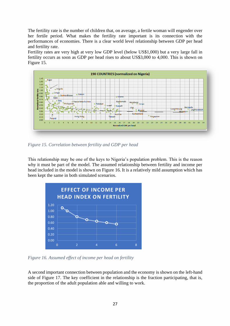
The fertility rate is the number of children that, on average, a fertile woman will engender over
her fertile period. What makes the fertility rate important is its connection with the
performances of economies. There is a clear world level relationship between GDP per head
and fertility rate.
Fertility rates are very high at very low GDP level (below US$1,000) but a very large fall in
fertility occurs as soon as GDP per head rises to about US$3,000 to 4,000. This is shown on
Figure 15.
Figure 15. Correlation between fertility and GDP per head
This relationship may be one of the keys to Nigeria’s population problem. This is the reason
why it must be part of the model. The assumed relationship between fertility and income per
head included in the model is shown on Figure 16. It is a relatively mild assumption which has
been kept the same in both simulated scenarios.
Figure 16. Assumed effect of income per head on fertility
A second important connection between population and the economy is shown on the left-hand
side of Figure 17. The key coefficient in the relationship is the fraction participating, that is,
the proportion of the adult population able and willing to work.
0.00
0.20
0.40
0.60
0.80
1.00
1.20
0 2 4 6 8
EFFECT OF INCOME PER HEAD INDEX ON FERTILITY

28
Figure 17. The model’s second view: labour supply, fertility and growth
In both scenarios, the model keeps this coefficient constant, but it is likely that as economies
develop more people, especially more women, would seek employment.
Figure 18.The capital, production and income view
The view displayed on Figure 18 describes the model’s production process. It is assumed that
output is a fixed proportion of the stock of productive capital. The connection between capital
and output, the capital output ratio, is one of the few major model parameters. The capital
output ratio is a time parameter. It is the number of years it takes for capital to return its value.
The model assumes a value of 3 years. The second key parameter of the production process is
the average capital lifetime. It is also a key parameter because it directly affects the value of
the stock of productive capital through its draining rate. In the base and best scenario, the model
assumes a value of respectively 25 and 30 years for this parameter. Another important
assumption in the model is a structural assumption. It is the assumption that the capital stock
LABOUR SUPPLY,FERTILITY,GROWTH
Population
total
Fraction
dependent
<VERY YOUNG
(0-4)>
<OLD (65
over)>
<ADULT
(25-64)>
<SCHOOL AGE
(5-14)>
Labour supply to
the economy
Fractionparticipating
<YOUNG ADULT
(15-24)>
Initial fertilityrate
Fertility rate
Indicated impact of
income per head on
fertility rate
Lookup effect onfertility
Delay impactingon fertility
<Income per
head index>
Initial
population
Initial labour
supply
GDPfc index
<Initial
GDPfc><GDP at factor
costs>
<PRODUCTIVE
CAPITAL><Investment>
<Depreciation>
Net change in
productive capital
Fractional change in
productive capital
GDP growth
Averagetime
Initial growth
PRODUCTIVE
CAPITAL
Initial
productive
capital
Investment
Depreciation
Averagecapitallifetime
Capitaloutputratio
GDP at market
pricesNational
income
Disposable
income
Savings
Propensityto save
Labour
requirement
Initial labour
required per M$
capital
Labour
available
Private
investment
Investmenteffectiveness
unemployment
CAPITAL, PRODUCTION & INCOME
Productive
capital index
InitialGDPfc
Labouravailability
ratio
Initial labourdemand
<Initial
productive
capital>
GDP atfactor costs
<VAT> <Labour
supply to the
economy>
Labour
ratio
Labour requirement
multiplier
Lookuplabour
required
Labour
required per
M$ capital
B$ CAPITALM$perB$
B$ private
investment
B$
Investment
B$ Government
investment
B$
Depreciation
<M$
per
B$>
<M$ per B$>B$ GDPfc
B$ GDPmp
B$ NI
B$ DI
<Private
transfers>
<Government
investment>
<Debt
servicing
domestic>
<Government tax
revenue><M$ total
subsidies>
Net
investment
<Investment>
<Depreciation>
B$ net
investment
<M$ per B$>
Initial
unemployment

29
determines the economy’s labour requirement. There exists initially in the economy a given
demand for labour: the labour required to operate the capital stock.
This initial labour demand is calculated as the difference between the volume of labour
population supplies to the economy and the level of unemployment. In addition, the model
assumes that, as the stock of capital renews itself through the replacement of depreciated
equipment, a labour-saving effect takes place as a result of the technical progress embodied
into new acquired capital. This tends to reduce labour demand. The critical parameter in this
relationship is the labour required per US$ millions of capital. The critical functional
relationship is the relation between productive capital index and labour requirement multiplier.
This relationship, however, was not activated in simulations.
The model also includes a labour availability ratio. This is a parameter between 0 and 1 the
purpose of which is to simulate in a simple way the impact of any disruption in the flow of
labour to the production process.
Figure 19 displays the fourth view of the model. This is a simple and straightforward view
which calculates the national income per head. The model requires an index of national income
per head. This index is calculated from the initial values of population and national income.
Figure 19. Fourth model view: the national income per head
Figure 20 shows the calculation of government revenue. This fifth model view depicts
another straightforward arithmetic.
National incomeper head
<Nationalincome>
$ per $million
<Populationtotal>
Initial nationalincome
Population totalinitial Initial national
income per head
<Initialadult>
<Initialold>
<Initialschoolage>
<Initialvery
young><Initialyoungadult>
Income perhead index
INCOME PER HEAD
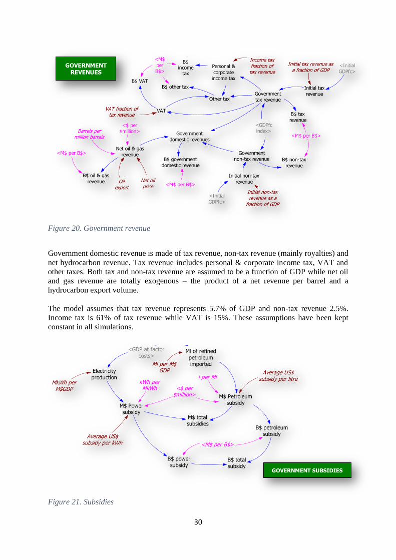
30
Figure 20. Government revenue
Government domestic revenue is made of tax revenue, non-tax revenue (mainly royalties) and
net hydrocarbon revenue. Tax revenue includes personal & corporate income tax, VAT and
other taxes. Both tax and non-tax revenue are assumed to be a function of GDP while net oil
and gas revenue are totally exogenous – the product of a net revenue per barrel and a
hydrocarbon export volume.
The model assumes that tax revenue represents 5.7% of GDP and non-tax revenue 2.5%.
Income tax is 61% of tax revenue while VAT is 15%. These assumptions have been kept
constant in all simulations.
Figure 21. Subsidies
Government
domestic revenues
Personal &
corporate
income tax
VAT
Net oil & gas
revenue
Oilexport
Net oilprice
Initial tax revenue asa fraction of GDP
Income taxfraction oftax revenue
VAT fraction oftax revenue
GOVERNMENTREVENUES
Barrels permillion barrels
B$income
tax
B$ VAT
<M$
per
B$>
B$ tax
revenue
B$ oil & gas
revenue
<M$ per B$>
B$ government
domestic revenue
Government
tax revenue
Government
non-tax revenue
<M$ per B$>
<Initial
GDPfc>
Initial tax
revenue
Initial non-taxrevenue as a
fraction of GDP
<M$ per B$>
B$ non-tax
revenue
<$ per
$million>
Other tax
B$ other tax
<Initial
GDPfc>
Initial non-tax
revenue
<GDPfc
index>
M$ totalsubsidies
Ml of refinedpetroleumimported
Average US$subsidy per kWh
Electricityproduction
<GDP at factorcosts>
MkWh perM$GDP
Ml per M$GDP
M$ Petroleumsubsidy
M$ Powersubsidy
Average US$subsidy per litrel per Ml
kWh perMkWh
B$ powersubsidy
B$ petroleumsubsidy
B$ totalsubsidy
<M$ per B$>
GOVERNMENT SUBSIDIES
<$ per$million>

31
The model includes both petrol and electricity subsidies. Both imported petroleum products
and electricity production are GDP related and the model assumes a decreasing subsidy per
kWh of electricity and per litre of refined petroleum consumed.
Figure 22 displays one of the model’s most important views: government expenditures and
indebtedness. Government expenditures include three components: consumption, investment
and debt servicing. The model assumes that government consumption and investment both
depend upon government domestic revenue and that the budget is in surplus or deficit whether
or not domestic revenue exceeds expenditures. Government propensity to consume and to
invest are two important parameters driving this structure.
Figure 22. Government expenditures and indebtedness
In the base case the model assumes that government propensity to consume falls slowly from
70% of revenue at the beginning of the simulation period to 40% at the end while propensity
to invest remains constant at 30% of revenue yearly. In contrast, in the best case, government
propensity to consume falls more rapidly to 25% at the end of the period while propensity to
invest more than double from 30% to 63%.
Budget deficits are financed by both the domestic public debt and the foreign public debt
according to an assumed share. In the base case, the sharing is on a 50/50 basis, in the best
case, the share of the domestic debt grows from 65% to 85%. Each debt pays interest which
add into total debt servicing and reimburses the principal borrowed. The model assumes a
constant foreign interest rate which is right as the foreign interest rate is truly an exogenous
parameter and a constant domestic interest rate which is wrong. One of the additional structures
required is one that would endogenously determine the domestic interest rate.
The penultimate view of the model is shown on Figure 23.
PUBLIC
DOMESTIC
DEBT
Initial publicdomestic debt
Domestic debtmaturity
Principal
repayment
domestic
Deficitfinancingdomestic
Domesticdebt share
Interest paid on
domestic debt
Interest rate ondomestic debt
PUBLIC
FOREIGN
DEBT
Initial publicforeign debt
Deficit
financing
foreign
Principal
repayment
foreign
Maturityforeigndebt
Interest paid on
foreign debt
Interest rateon foreign debt
<Exchange
rate
index>Governmentexpenditures
Government
surplus/deficit
Debt
servicing
total
Government
consumption
expenditures Government
investment
Governmentpropensity to
consume
Governmentpropensity to
invest
GOVERNMENTEXPENDITURES
&INDEBTEDNESS
Debt servicing
domestic
Debt servicing
foreign
<M$ total
subsidies>
<Government
domestic
revenues>
B$ gov.
surplus/deficit
<M$ per B$>
B$ government
expenditures
<Government
expenditures>
B$ total
debt service
<M$ per B$>
B$ gov.
investment
B$ gov.
consumption
<M$ perB$>
B$ foreign
debt
B$ domestic
debt
<M$perB$>
<M$perB$>
B$ foreign
interest
<M$perB$>
B$domesticinterest
B$ total
debt
<B$ foreign
debt>
B$ interest
total
<B$ foreign
interest>
<B$ GDPfc>
Debt to GDP
Debt service per
unit of revenue

32
Figure 23. Import, export and the diaspora
This view calculates import, non-oil export and the Nigerian diaspora’s remittances. Both
import and non-oil export are assumed to be a function of GDP with an added multiplier effect
resulting from the fluctuations of the exchange rate. As the naira appreciates (depreciates)
import become cheaper (dearer) and tend to increase (fall). The same exchange rate effect but
inversed applies to export, but the other way around: a deteriorating exchange rate favours
export. But even with the best possible exchange rate conditions, exportable goods must first
be produced before they are shipped. This is why the model also includes a capital multiplier
of non-oil export.
The model also assumes that there are 15 million Nigerians in the diaspora and that they remit
an average of US$1,700 per year.
The ninth and last view of the model is shown on Figure 24. It depicts the dynamic adjustment
of the exchange rate as a function of the variations in the stock of foreign exchange as was
explained earlier in the text. The exchange rate is assumed to be worth 380 naira per US dollar
at the beginning of the simulation period.
INTERNATIONALTRADE &
REMITTANCES
<Productivecapital index>
Lookupcapitalexport
multiplier
Initialpropensityto export(non-oil)
Capitalmultiplierof non-oil
export
NIGERIANSIN
DIASPORA
Initialdiaspora
Net change indiaspora
Net changefraction diaspora
Averageunit
remittance
Privatetransfers
Exchangerate
multiplierof import
Lookupexchange
rate importmultiplier
<Exchangerate index>
Total imports
Initialpropensityto import
<GDP at factorcosts>
B$ imports
<M$ per B$>
B$ privatetransfers
Non-oilexports
<GDP at factorcosts>
Exchange ratemultiplier of
non-oil export
Lookupexchange rate
exportmultiplier
B$ non-oilexports
<$ per$million>

33
Figure 24. The dynamic adjustment of the exchange rate
d. Assumptions, Scenarios and Simulations The model simulates from the first day of 2021 to the last day of 2050. Its time period is
the year and its financial data are measured in US dollars if stocks are concerned or in
US dollars per year if they are flows. A multitude of scenarios can be created and
simulated as the model requires 258 numerical data to simulate.
It takes less than a second to simulate the model, but significantly more time is required
to define a scenario and even more to analyze the results produced. It is important for
model users to learn how to define interesting or relevant scenarios and to be prepared to
spend the right amount of time to understand the results the model generates. The power
and speed of computers keep increasing while our own reasoning ability remains more
or less constant.
In order to facilitate the preparations of scenarios and data entry, the model is
accompanied by a data entry workbook called MODEL DATA PCDI.xlsx which initially
includes five worksheets: TITLE, DATA, DATA ENTRY, DATA CAPTURE and
DATA SHEET TEMPLATE.
Before simulating, the model reads worksheet DATA to capture the numerical
assumptions it requires to compute the model. The results of the simulation are saved in
a Vensim .vdf file named as specified by the model user in the data entry box under
‘Simulation results file name’.
Data are entered using worksheet DATA ENTRY. They are simultaneously saved on
worksheet DATA CAPTURE. Copy numerical values only from DATA CAPTURE and
paste special (data and formats) on a DATA SHEET TEMPLATE to save your scenario.
Rename worksheet ‘DATA SHEET TEMPLATE’: ‘DATA’ when ready to simulate.
FOREX
RESERVESForex in Forex out
Initialexchange
rateChange in
rate of
exchange
Timeadjustingexchange
rate
Desiredexchange
rate
Forex stockcoverage
Relative
forex stock
gap
Impact on
exchange rate
Lookup forexreserves
impact onexchange rate
Desired forex
reserves
FOREX RESERVES& THE EXCHANGE
RATE
Initialforeign
exchangereservesExports
RATE OF
EXCHANGE
<Net oil
& gas
revenue>
Total forex
demand
Forex available
<TIME STEP>
Exchange
rate index
<Private
transfers>
<Total
imports>
<Non-oil
exports>
<Debt servicing
foreign>
B$ forex
reserves
<FOREX
RESERVES>
<M$ per B$>
B$ desired
forex
<M$ per B$>
B$ forex inB$ forex out
<Forex out>
Government
surplus
<Government
surplus/deficit>

34
The results presented in the section below are the outcome of two scenarios: base and
best. A detailed list of all numerical data running each scenario is given in the data entry
workbook. A detailed description of each scenario together with their assumptions is
provided in the users’ guide.
CHAPER 5: ANALYSIS OF PRELIMINARY RESULTS The results of any simulation are presented in 13 views, 35 graphs and 6 tables. Results are
displayed on specific views of the Vensim model file. Simulation results are loaded invoking
Windows -> Control panel -> Dataset and selecting the dataset name(s) as earlier defined by
the user.
Another series of 13 views and 18 graphs are comparative results. They display on the same
graph the simulation results of any two (or more) loaded result files. Such graphs are very
useful to assess policy impacts provided scenarios have been properly defined changing only
one assumption at a time. What is discussed in this section is the comparison of scenarios base
and best.
It is important to keep in mind that the purpose of long-term models cannot be to generate
accurate predictions. The uncertainties are far too many and the range of possibilities much too
wide. Rather, long-term models are useful to indicate trends or directions of change, shapes
being more important than the actual data which constitute them.
The first graph displayed on Figure 25 can be interpreted as a quality indicator for the scenario.
What is compared is the ratio of debt to GDP in both scenarios. Debt to GDP is the ratio of a
stock to a rate. Its unit is therefore a time period, here the year.

35
Figure 25. Scenario comparison. Debt to GDP ratio
The comparison leads to a straightforward conclusion. Although the base scenario gives rise to
an indebtedness situation equivalent to less than half a year of GDP, which is manageable, the
trend is worrying. In contrast, the best scenario achieves a reversal in relative indebtedness
with a debt GDP ratio lower at the end of the period than at the beginning.
Debt to GDP
.6
.45
.3
.15
0
2021 2025 2029 2033 2037 2041 2045 2049
Time (Year)
Yea
r
Debt to GDP : AGENDA 2050 BASE
Debt to GDP : AGENDA 2050 BEST
DEBT TO GDP RATIO (year)

36
Figure 26. Population and national income
The left-hand side of Figure 26 shows the simulated evolution of population while the right-
hand side of the figure displays the behaviour over time of Nigeria’s national income (in US$
billion per year).
Because the model assumption that connects fertility to income per head is rather moderate, by
the end of the simulation period the model does not generate a large population difference
between the two scenarios. The base scenario gives 427 million compared to 416 million for
the best scenario. The difference is 11 million. A population reduction of 11 million is relatively
marginal for Nigeria. Yet it is a little more than the present population of Switzerland.
A much larger improvement is observed as far as the national income is concerned. From an
initial value of US$423 billion at the beginning of the simulation period, the base scenario
reaches US$763 billion at the end while the best scenario attains US$1360 billion. The
difference in favour of the best scenario is considerable: US$597 billion or 1.8 times what the
base scenario is capable of achieving.
POPULATION (people) & NATIONALINCOME (US$ billion)
Population total
500 M
375 M
250 M
125 M
0
2021 2025 2029 2033 2037 2041 2045 2049
Time (Year)
peo
ple
Population total : AGENDA 2050 BASE
Population total : AGENDA 2050 BEST
B$ NI
2000
1500
1000
500
0
2021 2025 2029 2033 2037 2041 2045 2049
Time (Year)
B$
/Yea
r
B$ NI : AGENDA 2050 BASE
B$ NI : AGENDA 2050 BEST

37
Figure 27. Unemployment
When unemployment is considered, a massive difference between both scenarios is observed.
From a starting level of 26 million unemployed or under-employed people at the beginning of
the simulation period, the model produces at the end of the period a very large difference of 61
million people between both scenarios. In the base scenario, in spite of a fall in unemployment
to about 18 million over the first ten years of the period, 44 million people are unemployed at
the end of the period. In sharp contrast, the best scenario shows a negative unemployment of
17 million. That means that Nigeria is projected to need an additional 17 million people in the
labour force to be able to run the economy. Several factors, however, which the scenarios have
not (but may have) considered come to mitigate this result. First it is likely that the Nigerian
population will produce a larger than simulated number of candidates for employment
especially from the female gender. Second the labour-saving impact of capital accumulation
has not been considered. All in all, while the best scenario undeniably offers a much better
perspective than its counterpart, the situation may not be as rosy as indicated by the simulation.
UNEMPLOYMENT (people)
unemployment
50 M
25 M
0
-25 M
-50 M
2021 2025 2029 2033 2037 2041 2045 2049
Time (Year)
peo
ple
unemployment : AGENDA 2050 BASE
unemployment : AGENDA 2050 BEST

38
Figure 28. National income per head
The gap in national income per head (US$ per person per year) between base and best scenario
is also significant although, in absolute value, both scenarios may be considered as generating
results below expectations. From US$2,200 per person per year at the beginning of the period,
at the end of the period, national income per head falls to US$1,790 per person per year in the
base scenario and raises to US$3,270 in the best scenario. The weight of the large and growing
Nigerian population is difficult to carry especially with an economy which is yet to reach
maturity.
NATIONAL INCOME PER HEAD (US$per people per year)
National income per head
4000
3250
2500
1750
1000
2021 2025 2029 2033 2037 2041 2045 2049
Time (Year)
$/(
Year*
peo
ple
)
National income per head : AGENDA 2050 BASE
National income per head : AGENDA 2050 BEST
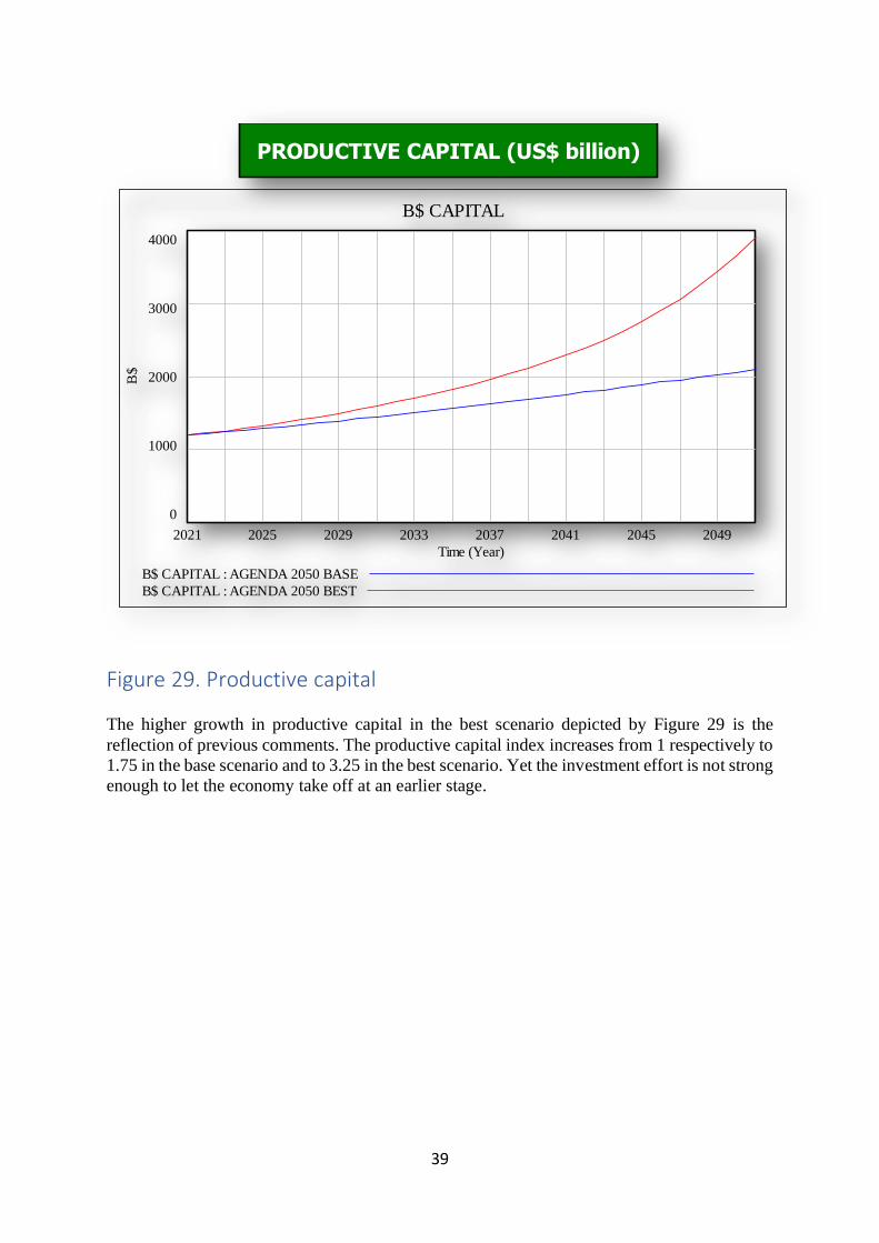
39
Figure 29. Productive capital
The higher growth in productive capital in the best scenario depicted by Figure 29 is the
reflection of previous comments. The productive capital index increases from 1 respectively to
1.75 in the base scenario and to 3.25 in the best scenario. Yet the investment effort is not strong
enough to let the economy take off at an earlier stage.
PRODUCTIVE CAPITAL (US$ billion)
B$ CAPITAL
4000
3000
2000
1000
0
2021 2025 2029 2033 2037 2041 2045 2049
Time (Year)
B$
B$ CAPITAL : AGENDA 2050 BASE
B$ CAPITAL : AGENDA 2050 BEST

40
Figure 30. Economic growth
This is perhaps the most important graph of both simulations. And what the graph conveys is
perhaps the most important message of the entire report.
The point of departure (2020) is a rate of economic growth of 1.78% and 2.31% respectively
for the base and best scenarios.
Figure 31 shows that in the first 10 years of the simulation period, between 2020 and 2030, the
base scenario only records marginal economic growth improvements. Then economic growth
falls. At the end of the period, growth is lower than it was at the start. This is the result of an
insufficient investment program over the period considered.
2025 1.92%
2030 1.97%
2035 1.94%
2040 1.85%
2045 1.77%
ECONOMIC GROWTH (%)
Fractional change in productive capital
.07
.0525
.035
.0175
0
2021 2025 2029 2033 2037 2041 2045 2049
Time (Year)
1/Y
ear
Fractional change in productive capital : AGENDA 2050 BASE
Fractional change in productive capital : AGENDA 2050 BEST

41
2050 1.74%
Figure 31. Base scenario: economic growth
Figure 32 clearly shows that the best scenario does much better.
2025 3.04%
2030 3.23%
2035 3.55%
2040 4.21%
2045 5.31%
2050 6.75%
Figure 32. Best scenario: economic growth
It also indicates that economic growth is the result of a long cumulative process which rests
upon recurrent streams of investments and the resulting build-up of productive capital over a
substantial period of time. This process cannot be successful without persistence and the
determination to build on what already exists rather than starting afresh at each change of
government. Nigeria requires the strict coordination of several medium-term plans and several
legislatures to achieve economic success.
Figure 33 is concerned with government revenues and expenditures.
Figure 33. Government revenues & expenditures
GOVERNMENT REVENUES & EXPENDITURES (US$ billion per year)
B$ government domestic revenue
200
150
100
50
0
2021 2025 2029 2033 2037 2041 2045 2049
Time (Year)
B$
/Year
B$ government domestic revenue : AGENDA 2050 BASE
B$ government domestic revenue : AGENDA 2050 BEST
B$ government expenditures
200
150
100
50
0
2021 2025 2029 2033 2037 2041 2045 2049
Time (Year)
B$
/Year
B$ government expenditures : AGENDA 2050 BASE
B$ government expenditures : AGENDA 2050 BEST

42
Unsurprisingly in both areas – revenues and expenditures, the best scenario shows higher
performances than the base. The effect on budget surplus/deficit is analysed in the next graph.
Figure 34. Government surplus / deficit
In the base scenario, government is incapable of keeping its budget under control and the
budget deficit grows exponentially to reach over US$47 billion at the end of the simulation
period. In sharp contrast, in the best scenario, government keeps public indebtedness under
control and, while still in deficit, toward the end of the period, a reduction in deficit is observed.
In the best scenario, the 2050 deficit is about US$8 billion, almost six times less than in the
base scenario.
B$ gov. surplus/deficit
0
-12.5
-25
-37.5
-50
2021 2025 2029 2033 2037 2041 2045 2049
Time (Year)
B$
/Year
"B$ gov. surplus/deficit" : AGENDA 2050 BASE
"B$ gov. surplus/deficit" : AGENDA 2050 BEST
GOVERNMENT SURPLUS / DEFICIT (US$ billion per year)

43
Figure 35. Government debts
When a country’s currency is weak, it is much better for government to put emphasis on
domestic rather than on foreign indebtedness. This is what Figure 35 illustrates. On domestic
debt, the divergence between both scenarios is only noticeable in the last five years of the
simulation as both debts grow in parallel for most of the period. Domestic debt is US$56.4
billion in 2020 and raises to reach respectively US$163 billion and US$165 billion in the base
and best scenario. Yet, at the end of the period, public domestic debt in the base scenario has
reached US$228 billion while in the best scenario the growth is slower, and the debt stock
stands at US$194 billion.
A vastly different situation is observed as far as the public foreign debt is concerned. While in
the base scenario, the foreign debt grows unabated from US$28 billion to over US$171 billion
at the end of the period, in the best scenario foreign debt grows moderately to US$69 billion in
2040 then starts declining to US$49 billion at the end of the period.
B$ domestic debt
300
225
150
75
0
2021 2025 2029 2033 2037 2041 2045 2049
Time (Year)
B$
B$ domestic debt : AGENDA 2050 BASE
B$ domestic debt : AGENDA 2050 BEST
B$ foreign debt
200
150
100
50
0
2021 2025 2029 2033 2037 2041 2045 2049
Time (Year)
B$
B$ foreign debt : AGENDA 2050 BASE
B$ foreign debt : AGENDA 2050 BEST
GOVERNMENT DEBTS (US$ billion)

44
Figure 36. Debt servicing
Debt servicing is a direct consequence of the debt situation. This is shown on Figure 36. As
both graphs clearly show, the burden of the debt is much easier to carry in the best scenario
than it is in the base scenario. The graph on the left-hand side shows how vastly the debt service
profiles of both scenarios differ from each other. This is another way to measure the effects of
good public management. In the base scenario total debt service grows exponentially from
US$7.5 billion at the beginning of the period to over US$66 billion at the end of the period
while in the best scenario debt servicing reaches a peak of only US$25 billion in 2047 then
declines to US$22.3 billion at the end of the period.
The graph on the right-hand side displays the share of government revenue that is allocated to
service the debt. In the base scenario this ratio grows from 19% at the beginning of the period
to over 100% at the end. This is a clearly untenable situation in which a country would have to
borrow to service its debt. In sharp contrast, in the best scenario, the ratio remains within a
range of 18/26% to finally fall back to 19% at the end of the period.
B$ total debt service
70
52.5
35
17.5
0
2021 2025 2029 2033 2037 2041 2045 2049
Time (Year)
B$
/Year
B$ total debt service : AGENDA 2050 BASE
B$ total debt service : AGENDA 2050 BEST
GOVERNMENT DEBT SERVICE (US$ billion per year)
Debt service per unit of revenue
2
1.5
1
.5
0
2021 2025 2029 2033 2037 2041 2045 2049
Time (Year)
Dm
nl
Debt service per unit of revenue : AGENDA 2050 BASE
Debt service per unit of revenue : AGENDA 2050 BEST

45
Figure 37. International trade
In the model, imports and non-oil exports depend upon GDP and the exchange rate. Non-oil
exports, however, also depend upon a third variable, the accumulation of productive capital.
An appreciation of the exchange rate makes the naira more expensive in terms of foreign
currency, discourages exports and boosts imports. Conversely a depreciation of the exchange
rate makes the naira cheaper in terms of foreign currency, boosts exports and discourages
imports. The left-hand side of Figure 37 reflects the fluctuations of the exchange rate, the
difference in position on the graph indicating the fact that economic growth is substantially
stronger in the best scenario. Also reflective of the difference in economic growth is the
evolution of non-oil exports. Starting at US$4 billion in both scenarios, non-oil exports reach
US$20 and US$50 billion respectively in the base and best scenarios. A better managed
economy results in multiplying export by a factor of 2.5.
B$ imports
80
60
40
20
0
2021 2025 2029 2033 2037 2041 2045 2049
Time (Year)
B$/Y
ear
B$ imports : AGENDA 2050 BASE
B$ imports : AGENDA 2050 BEST
B$ non-oil exports
50
37.5
25
12.5
0
2021 2025 2029 2033 2037 2041 2045 2049
Time (Year)
B$
/Year
"B$ non-oil exports" : AGENDA 2050 BASE
"B$ non-oil exports" : AGENDA 2050 BEST
IMPORT & NON-OIL EXPORT (US$ billion per year)
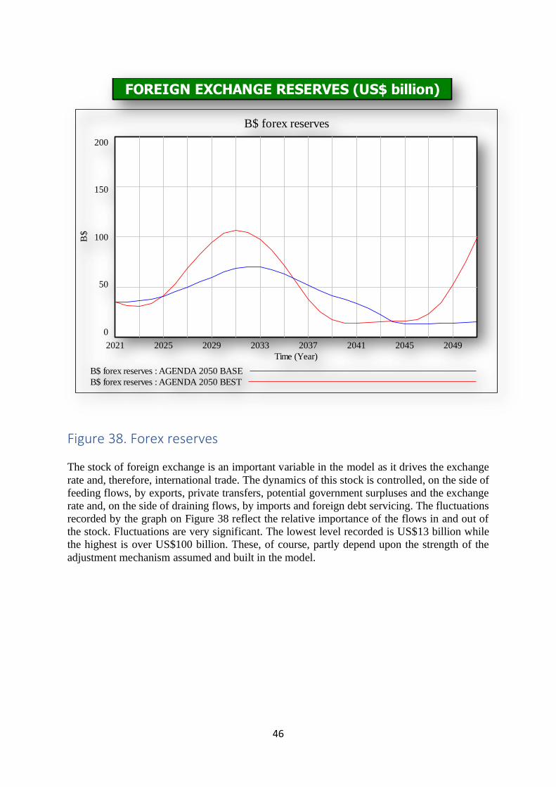
46
Figure 38. Forex reserves
The stock of foreign exchange is an important variable in the model as it drives the exchange
rate and, therefore, international trade. The dynamics of this stock is controlled, on the side of
feeding flows, by exports, private transfers, potential government surpluses and the exchange
rate and, on the side of draining flows, by imports and foreign debt servicing. The fluctuations
recorded by the graph on Figure 38 reflect the relative importance of the flows in and out of
the stock. Fluctuations are very significant. The lowest level recorded is US$13 billion while
the highest is over US$100 billion. These, of course, partly depend upon the strength of the
adjustment mechanism assumed and built in the model.
FOREIGN EXCHANGE RESERVES (US$ billion)
B$ forex reserves
200
150
100
50
0
2021 2025 2029 2033 2037 2041 2045 2049
Time (Year)
B$
B$ forex reserves : AGENDA 2050 BASE
B$ forex reserves : AGENDA 2050 BEST

47
Figure 39. The naira exchange rate
There is some convergence between Figure 38 and Figure 39 but the result generated by the
model is surprising and certainly counter-intuitive. One important lesson to learn from this
model’s result is that the exchange rate should certainly not be an exogenous variable in
economic models. Modelling the exchange rate in connection with the stock of foreign
exchange seems to be the right approach as past developments in the Nigerian economy seem
to support it.
First the results. The behavior over time is clearly cyclical. From 2021 to 2039/2040 the model
shows exchange rate stability in both scenarios. The starting point is ₦380 per US$. In the base
scenario, the exchange rate grows to ₦400/US$ in 2026 then falls to ₦344/US$ 10 years later
in 2036. It then rises again exponentially until the end of the period. In 2050 the exchange rate
stands at ₦1,562/US$, over 4 times its initial value.
RATE OF EXCHANGE
2000
1500
1000
500
0
2021 2025 2029 2033 2037 2041 2045 2049
Time (Year)
nair
a/$
RATE OF EXCHANGE : AGENDA 2050 BASE
RATE OF EXCHANGE : AGENDA 2050 BEST
THE EXCHANGE RATE naira per (US$)

48
In the best scenario the exchange rate rises faster to ₦426/US$ in 2025 then falls to ₦299/US$
10 years later in 2035 then climbs again to ₦2,516/US$ in 2049 but begins a turnaround in the
last year of the simulation to ₦1,494/US$. It is therefore a quite different behavior.
To be able to judge the validity of these results and the importance of the assumptions that
drive them, it is necessary to delve into the structure of the model.
The driver of the exchange rate’s dynamics is the ratio between forex reserves and desired
forex reserves. To put it bluntly the ratio between what we have and what we want. This is a
very common approach in system dynamics. If the ratio is greater than one it means that we
have more forex stock than what we want. It is therefore time to lower its price to clear the
excess. Lowering the price means to make the US dollar cheaper in terms of naira which means
for the naira exchange rate to appreciate. The table on the left-hand side of Figure 40 which is
extracted from the data entry worksheet, shows that when X grows above 1, Y, the exchange
rate multiplier falls below 1.
45. TABLE 23
X Y
RELATIVE EXCHANGE
RATE
FOREX
STOCK IMPACT
GAP [Line 46] [Line 47]
0.1 1.5
1.0 1
2.0 0.8
4.0 0.6
8.0 0.5
12 0.4
15 0.4
Figure 40. Extract from the data entry worksheet. Relationship forex stock – exchange rate
Conversely, if the ratio is lower than 1 it means that we have less forex stock than what we
want. It is therefore time to increase its price so as to reduce or stop stock drainage. Increasing
the price means to make the US dollar dearer in terms of naira which means for the naira
exchange rate to depreciate.
Figure 41 shows, for each scenario, the coefficient by which the exchange rate is multiplied.
When it is higher than 1 the exchange rate depreciates, when it is lower, it appreciates. The
superiority of the best scenario then becomes very clear.
0
0.5
1
1.5
2
0.0 5.0 10.0 15.0 20.0
IMPACT OF RELATIVE FOREX STOCK GAP ON EXCHANGE
RATE

49
Figure 41. The exchange rate multiplier
CHAPTER 6: FURTHER MODEL DEVELOPMENT - DYNAMIC INPUT-OUTPUT MODEL Significant model improvement would result if the following developments were implemented:
production disaggregation using dynamic input-output modelling; modelling of education,
energy, the environment and the informal economy; endogenous determination of the Interest
rate. In addition, there always remains the possibility of modelling in more depth some selected
areas as may be required.
As a preview of what can be done to improve the existing model, the following description of
how dynamic input-output modelling can be done using system dynamics illustrates the
powerful capability of this modelling and simulation tool to build complex computable
structures. The steps of this dynamic process inspired by supply chain management are detailed
below.
Any sector of a global economy purchases inputs to produce. It also sells its own products to
various clients. Clients are either the sector itself, which needs to consume some of its own
output to produce, other sectors of the economy which are procuring inputs, or final consumers.
Industries do not immediately respond to orders as they come, neither do they directly sell what
they produce. Rather, industries accumulate orders in a stock of unfilled orders which they
manage in line with their inventory (the stock of what they produce).
Impact on exchange rate
2
1.4
.8
2021 2029 2037 2045
Time (Year)
Dm
nl
Impact on exchange rate : AGENDA 2050 - BASE
Impact on exchange rate : AGENDA 2050 BEST
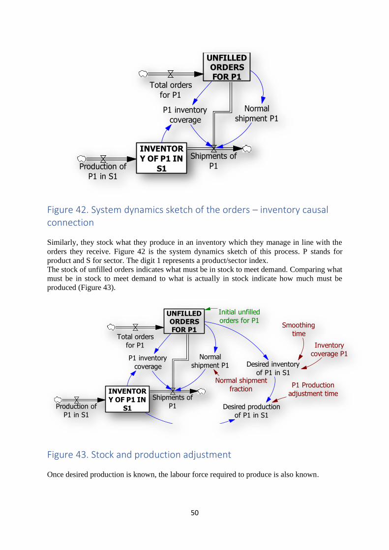
50
Figure 42. System dynamics sketch of the orders – inventory causal connection
Similarly, they stock what they produce in an inventory which they manage in line with the
orders they receive. Figure 42 is the system dynamics sketch of this process. P stands for
product and S for sector. The digit 1 represents a product/sector index.
The stock of unfilled orders indicates what must be in stock to meet demand. Comparing what
must be in stock to meet demand to what is actually in stock indicate how much must be
produced (Figure 43).
Figure 43. Stock and production adjustment
Once desired production is known, the labour force required to produce is also known.
INVENTOR
Y OF P1 IN
S1Production of
P1 in S1
Shipments of
P1
UNFILLEDORDERSFOR P1
Total orders
for P1
P1 inventory
coverage
Normal
shipment P1
INVENTOR
Y OF P1 IN
S1Production of
P1 in S1
Shipments of
P1
UNFILLEDORDERSFOR P1
Total orders
for P1
Initial unfilled
orders for P1
Desired inventory
of P1 in S1
Desired production
of P1 in S1
P1 inventory
coverage
Normal
shipment P1
Normal shipment
fractionP1 Production
adjustment time
Inventory
coverage P1
Smoothing
time

51
Figure 44. Labour force dynamics The volume of labour to hire is obtained by comparing desired labour force to existing labour
force (Figure 44).
Labour is one of the components that sectors require to produce. The others are the material
inputs to the production process. These inputs are supplied by the other sectors of the economy
then stocked as shown on Figure 45.
Figure 45. Material input procurement
This structure is replicated as many times as there are sectors in the economy.
The above analysis is conducted in volume. What is measured are quantities or volumes. The
value analysis is done from the calculation of accounting costs for inputs and the determination
of selling prices for outputs. Accounting costs are calculated dividing a stock value by a stock
volume. They are needed to determine the costs of material usages. Figure 46 includes input
stocks and inventory valuations and shows the overall causal structure of a single sector. The
four highlighted feedback loops are balancing as the growth of the system results from inter-
INVENTOR
Y OF P1 IN
S1
Initial P1
inventory in S1
Production of
P1 in S1Desired production
of P1 in S1
Desired labour
in S1
LABOUR
EMPLOYED
IN S1
Initial labour
employed in S1
Net hiring in
S1
P1 Production
from S1 labour
Labour
productivity in S1 Time adjusting
labour
INVENTOR
Y OF P1 IN
S1Production of
P1 in S1
Shipments of
P1
UNFILLEDORDERSFOR P1
Total orders
for P1
Desired inventory
of P1 in S1
P2 STOCK
IN S1
P2 Deliveries
from S2
Desired stock of
P2 in S1
I/O ratio P2 per
unit of P1
S1 Orders for
P2
P1 Production
from P2 stock
P1 inventory
coverage
<S2 Orders for
P1>

52
industry orders which constitute reinforcing loops as they trigger more demand and more
production in each sector. Replicating this structure as many times as there are products and
sectors in the economy using the indexing capability of Vensim DSS and feeding the structure
with the required data produces what constitutes in our opinion the best representation of
dynamic inter-industry linkages.
Figure 46. Complete causal structure of a single sector
APPENDIX 1: MODEL EQUATIONS The 255 equations of the model are listed below.
1. Initial growth = 0.0175 1/Year
2. Net change in productive capital = Investment-Depreciation M$/Year
3. Fractional change in productive capital = Net change in productive capital /
PRODUCTIVE CAPITAL 1/Year
4. GDP growth = TREND (GDP at factor costs, Average time, Initial growth) 1/Year
5. Average time = 1 Year
6. Forex in = Exports + Private transfers + (Government surplus * Exchange rate index)
M$/Year
7. Government surplus = IF THEN ELSE ("Government surplus/deficit" > 0,
"Government surplus/deficit", 0) M$/Year
8. Debt to GDP = B$ total debt / B$ GDPfc Year
9. B$ desired forex = Desired forex reserves / M$ per B$ B$
10, "Government non-tax revenue" = "Initial non-tax revenue" * GDPfc index
M$/Year
11. B$ forex out = Forex out / M$ per B$ B$/Year
12. Government tax revenue = Initial tax revenue * GDPfc index M$/Year
13. B$ forex in = Forex in / M$ per B$ B$/Year
14. GDPfc index = GDP at factor costs / Initial GDPfc Dmnl
15. "Initial non-tax revenue" = Initial GDPfc * "Initial non-tax revenue as a fraction of
GDP" M$/Year
INVENTORYOF P1 IN S1
Initial P1inventory
in S1
Production ofP1 in S1
Shipments ofP1
UNFILLEDORDERSFOR P1
Totalordersfor P1
Initial unfilledorders for P1
Desired inventoryof P1 in S1
Desiredproduction of
P1 in S1
Desiredlabour in S1
LABOUREMPLOYED
IN S1
Initial labouremployed in S1
Net hiringin S1
P1 Productionfrom S1 labour
Labourproductivity
in S1
P2 STOCKIN S1
Initial stockof P2 in S1
Usage ofP2 in S1
P2 Deliveriesfrom S2
Desired stock ofP2 in S1
I/O ratio P2 perunit of P1
S1 Ordersfor P2
P1 Productionfrom P2 stock
Finaldemandfor P1
P1 inventorycoverage
Normalshipment P1
Normalshipmentfraction
<I/O ratio P2per unit of P1> P1 Production
adjustment time
Inventorycoverage P1
Smoothingtime
P2 Stockadjustment
time
<S2 Ordersfor P1>
P2 STOCKVALUE IN S1P2 Material
purchase
P2usagecost
Initial P2 stockvalue in S1
P2Accounting
cost
P1INVENTORY
VALUE
Initial P1inventory value
P1 productionvalue
P1 salesvalue P1 selling
price
SECTOR 1
PRODUCT 1<TIMESTEP>
Timeadjustinglabour
<P2 sellingprice>
B
B
B
B

53
16. B$ interest total = B$ domestic interest + B$ foreign interest B$/Year
17. B$ domestic interest = Interest paid on domestic debt / M$ per B$ B$/Year
18. B$ foreign debt = PUBLIC FOREIGN DEBT / M$ per B$ B$
19. B$ foreign interest = Interest paid on foreign debt / M$ per B$ B$/Year
20. Initial population = INITIAL (Population total) people
21. "B$ gov. investment" = Government investment / M$ per B$ B$/Year
22. B$ total debt = B$ domestic debt + B$ foreign debt B$
23. "B$ gov. consumption" = Government consumption expenditures / M$ per B$
B$/Year
24. B$ total debt service = Debt servicing total / M$ per B$ B$/Year
25. Initial labour supply = INITIAL (Labour supply to the economy) people
26. "Non-oil exports" = GDP at factor costs * "Initial propensity to export (non-oil)" *
"Exchange rate multiplier of non-oil export" * "Capital multiplier of non-oil export"
M$/Year
27. B$ domestic debt = PUBLIC DOMESTIC DEBT / M$ per B$ B$
28. Initial unemployment = INITIAL (unemployment) people
29. B$ government expenditures = Government expenditures / M$ per B$ B$/Year
30. B$ forex reserves = FOREX RESERVES / M$ per B$ B$
31. "B$ gov. surplus/deficit" = "Government surplus/deficit" / M$ per B$ B$/Year
32. Other tax = Government tax revenue - "Personal & corporate income tax" – VAT
M$/Year
33. B$ other tax = Other tax / M$ per B$ B$/Year
34. Net investment = Investment – Depreciation M$/Year
35. B$ net investment = Net investment / M$ per B$ B$/Year
36. Initial installed distribution capacity = 2000 MW
37. Initial installed production capacity = 4000 MW
38. M$ Power subsidy = Electricity production * Average US$ subsidy per kWh * kWh
per MkWh / "$ per $million" M$/Year
39. INSTALLED DISTRIBUTION CAPACITY = INTEG (Distribution capacity
added - Distribution capacity depreciated, Initial installed distribution capacity) MW
40. CULTIVATED LAND= INTEG (Land addition - Land erosion, Initial cultivated
land) ha
41. Distribution capacity added = 0 MW/Year
42. Distribution capacity depreciated = INSTALLED DISTRIBUTION CAPACITY *
Depreciation fraction distribution MW/Year
43. Initial cultivated land = 0 ha
44. Production capacity added = 0 MW/Year
45. Production capacity depreciated = INSTALLED PRODUCTION CAPACITY *
Depreciation fraction production MW/Year
46. Land addition = 0 ha/Year
47. INSTALLED PRODUCTION CAPACITY = INTEG (Production capacity added -
Production capacity depreciated, Initial installed production capacity) MW
48. Erosion fraction = 0 1/Year
49. Land erosion = CULTIVATED LAND * Erosion fraction ha/Year
50. Depreciation fraction production = 0 1/Year
51. Depreciation fraction distribution = 0 1/Year
52. Indicated impact of income per head on fertility rate = Lookup effect on fertility
(Income per head index) Dmnl
53. Government consumption expenditures = Government domestic revenues *
Government propensity to consume M$/Year

54
54. Disposable income = National income - Government tax revenue M$/Year
55. Change in rate of exchange = (Desired exchange rate - RATE OF EXCHANGE) /
Time adjusting exchange rate naira/$/Year
56. "Net oil & gas revenue" = (Oil export * Net oil price * Barrels per million barrels)
/ "$ per $million" M$/Year
57. Private transfers = NIGERIANS IN DIASPORA * Average unit remittance / "$ per
$million" M$/Year
58. GDP at market prices = GDP at factor costs + VAT - M$ total subsidies M$/Year
59. Initial tax revenue = Initial GDPfc * Initial tax revenue as a fraction of GDP
M$/Year
60. Government investment = Government domestic revenues * (Government
propensity to invest) M$/Year
61. "Government surplus/deficit" = Government domestic revenues - Government
expenditures M$/Year
62. Government expenditures = Government consumption expenditures + Government
investment + Debt servicing total + M$ total subsidies M$/Year
63. M$ Petroleum subsidy = Ml of refined petroleum imported * Average US$ subsidy
per litre * l per Ml / "$ per $million" M$/Year
64. "$ per $million" = 1e+06 $/M$
65. M$ total subsidies = M$ Petroleum subsidy + M$ Power subsidy M$/Year
66. kWh per MkWh = 1e+06 kWh/MkWh
67. l per Ml = 1e+06 l/Ml
68. B$ tax revenue = Government tax revenue / M$ per B$ B$/Year
69. Ml of refined petroleum imported = GDP at factor costs * Ml per M$ GDP
Ml/Year
70. Initial national income = INITIAL (National income) M$/Year
71. Initial national income per head = (Initial national income * "$ per $million") /
Population total initial $ / (Year*people)
72. "Initial non-tax revenue as a fraction of GDP" = GET XLS CONSTANTS
('MODEL DATA PCDI.xlsx', 'DATA', 'B29') Dmnl
73. Average US$ subsidy per kWh = GET XLS DATA ('MODEL DATA
PCDI.xlsx', 'DATA', '1', 'B45') $/kWh
74. Average US$ subsidy per litre = GET XLS DATA ('MODEL DATA PCDI.xlsx',
'DATA', '1', 'B44') $/l
B$ power subsidy = M$ Power subsidy / M$ per B$ B$/Year
75. Income per head index = National income per head / Initial national income per
head Dmnl
76. B$ government domestic revenue = Government domestic revenues / M$ per B$
B$/Year
77. B$ VAT = VAT / M$ per B$ B$/Year
78. "Personal & corporate income tax" = Government tax revenue * Income tax fraction
of tax revenue M$/Year
79. VAT= Government tax revenue * VAT fraction of tax revenue M$/Year
80. Population total initial = Initial very young + Initial school age + Initial young adult
+ Initial adult + Initial old people
81. "B$ non-tax revenue" = "Government non-tax revenue" / M$ per B$ B$/Year
82. B$ petroleum subsidy = M$ Petroleum subsidy / M$ per B$ B$/Year
83. National income per head = (National income * "$ per $million") / Population total
$ / people/Year
55
84. Government domestic revenues = "Net oil & gas revenue" + Government tax
revenue + "Government non-tax revenue" M$/Year
85. B$ total subsidy = B$ petroleum subsidy + B$ power subsidy B$/Year
86. MkWh per M$GDP = GET XLS DATA ('MODEL DATA PCDI.xlsx', 'DATA', '1',
'B43') MkWh/M$
87. Electricity production = GDP at factor costs * MkWh per M$GDP MkWh/Year
88. Ml per M$ GDP = GET XLS DATA ('MODEL DATA PCDI.xlsx', 'DATA', '1',
'B42') Ml/M$
89. National income = GDP at market prices + Debt servicing domestic + Private
transfers M$/Year
90. "Exchange rate multiplier of non-oil export" = Lookup exchange rate export
multiplier (Exchange rate index) Dmnl
91. Exports = "Non-oil exports" + "Net oil & gas revenue" M$/Year
92. B$ private transfers = Private transfers / M$ per B$ B$/Year
93. Forex out = MIN (MAX (Forex available, 0), Total forex demand) M$/Year
94. Interest paid on domestic debt = PUBLIC DOMESTIC DEBT * Interest rate on
domestic debt $/Year
95. Interest paid on foreign debt = PUBLIC FOREIGN DEBT * Interest rate on foreign
debt*Exchange rate index M$/Year
96. B$ imports = Total imports / M$ per B$ B$/Year
97. Debt servicing total = Debt servicing domestic + Debt servicing foreign M$/Year
98. "B$ non-oil exports" = "Non-oil exports" / M$ per B$ B$/Year
99. Total forex demand = Total imports + Debt servicing foreign M$/Year
100. Debt servicing domestic = Principal repayment domestic + Interest paid on
domestic debt M$/Year
101. Lookup exchange rate export multiplier = GET XLS LOOKUPS ('MODEL DATA
PCDI.xlsx', 'DATA', '54', 'B55') Dmnl
102. Total imports = GDP at factor costs * Initial propensity to import * Exchange rate
multiplier of import M$/Year
103. Deficit financing domestic = IF THEN ELSE ("Government surplus/deficit" < 0,
(-"Government surplus/deficit" * Domestic debt share), 0) M$/Year
104. Deficit financing foreign = IF THEN ELSE ("Government surplus/deficit" < 0, -
"Government surplus/deficit" * (1-Domestic debt share), 0) M$/Year
105. Principal repayment foreign = (PUBLIC FOREIGN DEBT / Maturity foreign
debt) * Exchange rate index M$/Year
106. Debt servicing foreign = Principal repayment foreign + Interest paid on foreign
debt M$/Year
107. Initial propensity to import = GET XLS CONSTANTS ('MODEL DATA
PCDI.xlsx', 'DATA', 'B30') Dmnl
108. Investment = (Private investment + Government investment) * Investment
effectiveness M$/Year
109. Government propensity to consume = GET XLS DATA ('MODEL DATA
PCDI.xlsx', 'DATA', '1', 'B37') Dmnl
110. NIGERIANS IN DIASPORA = INTEG (Net change in diaspora, Initial diaspora)
people
Government propensity to invest = GET XLS DATA ('MODEL DATA PCDI.xlsx',
'DATA', '1', 'B38') Dmnl
111. "Initial propensity to export (non-oil)" = GET XLS CONSTANTS ('MODEL
DATA PCDI.xlsx', 'DATA', 'B39') Dmnl

56
112. "Capital multiplier of non-oil export" = Lookup capital export multiplier
(Productive capital index) Dmnl
113. Lookup exchange rate import multiplier = GET XLS LOOKUPS ('MODEL
DATA PCDI.xlsx', 'DATA', '54', 'B31') Dmnl
114. Exchange rate multiplier of import = Lookup exchange rate import multiplier
(Exchange rate index) Dmnl
115. Average unit remittance = GET XLS DATA ('MODEL DATA PCDI.xlsx',
'DATA', '1', 'B53') $/people/Year
116. Lookup capital export multiplier = GET XLS LOOKUPS ('MODEL DATA
PCDI.xlsx', 'DATA', '68', 'B52') Dmnl
117. Initial diaspora = GET XLS CONSTANTS ('MODEL DATA PCDI.xlsx', 'DATA',
'B57') people
118. Net change fraction diaspora = GET XLS DATA ('MODEL DATA PCDI.xlsx',
'DATA', '1', 'B56') 1/Year
119. Net change in diaspora = NIGERIANS IN DIASPORA * Net change fraction
diaspora people/Year
120. B$ GDPmp = GDP at market prices / M$ per B$ B$/Year
121. B$ DI = Disposable income / M$ per B$ B$/Year
122. B$ GDPfc = GDP at factor costs / M$ per B$ B$/Year
123. B$ NI = National income / M$ per B$ B$/Year
124. "B$ oil & gas revenue" = "Net oil & gas revenue" / M$ per B$ B$/Year
125. B$ income tax = "Personal & corporate income tax" / M$ per B$ B$/Year
126. Labour requirement multiplier = Lookup labour required (Productive capital
index) Dmnl
127. B$ private investment = Private investment / M$ per B$ B$/Year
128. B$ Government investment = B$ Investment - B$ private investment B$/Year
129. B$ CAPITAL = PRODUCTIVE CAPITAL / M$ per B$ B$
130. B$ Depreciation = Depreciation / M$ per B$ B$/Year
131. M$ per B$ = 1000 M$/B$
132. B$ Investment = Investment / M$ per B$ B$/Year
133. Interest rate on domestic debt = GET XLS DATA ('MODEL DATA PCDI.xlsx',
'DATA', '1', 'B33') 1/Year
134. Interest rate on foreign debt = GET XLS DATA ('MODEL DATA PCDI.xlsx',
'DATA', '1', 'B36') 1/Year
135. Initial public foreign debt = GET XLS CONSTANTS ('MODEL DATA
PCDI.xlsx', 'DATA', 'B34') M$
136. Principal repayment domestic = PUBLIC DOMESTIC DEBT / Domestic debt
maturity M$/Year
137. Domestic debt maturity = GET XLS DATA ('MODEL DATA PCDI.xlsx',
'DATA', '1', 'B41') Year
138. Domestic debt share = GET XLS DATA ('MODEL DATA PCDI.xlsx', 'DATA',
'1', 'B32') Dmnl
139. PUBLIC FOREIGN DEBT = INTEG (Deficit financing foreign - Principal
repayment foreign, Initial public foreign debt) M$
140. PUBLIC DOMESTIC DEBT = INTEG (Deficit financing domestic - Principal
repayment domestic, Initial public domestic debt) M$
141. Maturity foreign debt = GET XLS DATA ('MODEL DATA PCDI.xlsx', 'DATA',
'1', 'B35') Year
142. Initial public domestic debt = GET XLS CONSTANTS ('MODEL DATA
PCDI.xlsx', 'DATA', 'B40') M$

57
143. Exchange rate index = RATE OF EXCHANGE / Initial exchange rate Dmnl
144. Labour required per M$ capital = Initial labour required per M$ capital * Labour
requirement multiplier people/M$
145. Labour requirement = PRODUCTIVE CAPITAL * Labour required per M$
capital people
146. Lookup effect on fertility = GET XLS LOOKUPS ('MODEL DATA PCDI.xlsx',
'DATA', '66', 'B67') Dmnl
147. Delay impacting on fertility = GET XLS CONSTANTS ('MODEL DATA
PCDI.xlsx', 'DATA', 'B65') Year
148. Lookup labour required = GET XLS LOOKUPS ('MODEL DATA PCDI.xlsx',
'DATA', '68', 'B69') Dmnl
149. Initial fertility rate = GET XLS CONSTANTS ('MODEL DATA PCDI.xlsx',
'DATA', 'B9') Dmnl
150. Total births expected = ("YOUNG ADULT (15-24)" + "ADULT (25-64)") *
Female ratio * Fertility rate people
151. Fertility rate = Initial fertility rate * DELAY1 (Indicated impact of income per
head on fertility rate, Delay impacting on fertility) Dmnl
152. GDP at factor costs = PRODUCTIVE CAPITAL / Capital output ratio * Labour
ratio M$/Year
153. Forex available = FOREX RESERVES / TIME STEP M$/Year
154. Labour ratio = Labour available / Labour requirement Dmnl
155. Actual effect of environmental degradation on life expectancy at birth = DELAY1
(Indicated effect of environmental degradation on life expectancy at birth, Delay
impacting on life expectancy) Dmnl
156. Initial labour required per M$ capital = Initial labour demand / Initial productive
capital people/M$
157. Indicated effect of environmental degradation on life expectancy at birth = Lookup
effect on life expectancy (Index of environmental degradation) Dmnl
158. Lookup effect on life expectancy (GET XLS LOOKUPS ('MODEL DATA
PCDI.xlsx', 'DATA', '63', 'B64')) Dmnl
159. Degradation unit per M$ GDP = GET XLS DATA ('MODEL DATA
PCDI.xlsx', 'DATA', '1', 'B59') unit/M$
160. Delay impacting on life expectancy = GET XLS CONSTANTS ('MODEL DATA
PCDI.xlsx', 'DATA', 'B62') Year
161. Environmental restoration budget = GET XLS DATA ('MODEL DATA
PCDI.xlsx', 'DATA', '1', 'B61') M$/Year
162. Unit restoration cost = GET XLS DATA ('MODEL DATA PCDI.xlsx', 'DATA',
'1', 'B58') M$/unit
163. Restoration rate = Environmental restoration budget / Unit restoration cost
unit/Year
164. Foreign debt maturity = GET XLS DATA ('MODEL DATA PCDI.xlsx', 'DATA',
'1', 'B35') Year
165. VAT fraction of tax revenue = GET XLS DATA ('MODEL DATA PCDI.xlsx',
'DATA', '1', 'B28') Dmnl
166. Income tax fraction of tax revenue = GET XLS DATA ('MODEL DATA
PCDI.xlsx', 'DATA', '1', 'B27') Dmnl
167. Initial foreign exchange reserves = GET XLS CONSTANTS ('MODEL DATA
PCDI.xlsx', 'DATA', 'B51') M$
168. Initial environmental degradation units = GET XLS CONSTANTS ('MODEL
DATA PCDI.xlsx', 'DATA', 'B60') unit
58
169. Share of domestic debt = GET XLS DATA ('MODEL DATA PCDI.xlsx', 'DATA',
'1', 'B32') Dmnl
170. Net oil price = GET XLS DATA ('MODEL DATA PCDI.xlsx', 'DATA', '1', 'B24')
$/bbl
171. Barrels per million barrels = 1e+06 bbl/Mbbl
172. Oil export = GET XLS DATA ('MODEL DATA PCDI.xlsx', 'DATA', '1', 'B25')
Mbbl/Year
173. Initial tax revenue as a fraction of GDP = GET XLS CONSTANTS ('MODEL
DATA PCDI.xlsx', 'DATA', 'B26') Dmnl
174. Degradation rate = GDP at factor costs * Degradation unit per M$ GDP unit/Year
175. ENVIRONMENTAL DEGRADATION UNITS = INTEG (Degradation rate -
Restoration rate, Initial environmental degradation units) unit
176. Index of environmental degradation = ENVIRONMENTAL DEGRADATION
UNITS / Initial environmental degradation units Dmnl
177. Initial life expectancy at birth = GET XLS CONSTANTS ('MODEL DATA
PCDI.xlsx', 'DATA', 'B11') Year
178. Life expectancy at birth = Initial life expectancy at birth Year
179. Life expectancy at 15 = Initial life expectancy at 15 Year
180. Life expectancy at 25 = Initial life expectancy at 25 Year
181. Deaths young adult = "YOUNG ADULT (15-24)" / Life expectancy at 15
people/Year
182. Life expectancy at 65 = Initial life expectancy at 65 Year
183. Initial life expectancy at 65 = GET XLS CONSTANTS ('MODEL DATA
PCDI.xlsx', 'DATA', 'B15') Year
184. Initial life expectancy at 15 = GET XLS CONSTANTS ('MODEL DATA
PCDI.xlsx', 'DATA', 'B13') Year
185. Initial life expectancy at 25 = GET XLS CONSTANTS ('MODEL DATA
PCDI.xlsx', 'DATA', 'B14') Year
186. Life expectancy at 5 = Initial life expectancy at 5 Year
187. Initial life expectancy at 5 = GET XLS CONSTANTS ('MODEL DATA
PCDI.xlsx', 'DATA', 'B12') Year
188. Birth fraction = Yearly births / Population total 1/Year
189. Death fraction = Total deaths / Population total 1/Year
190. Population total = "VERY YOUNG (0-4)" + "SCHOOL AGE (5-14)" + "YOUNG
ADULT (15-24)" + "ADULT (25-64)" + "OLD (65 over)" people
191. Average capital lifetime = GET XLS CONSTANTS ('MODEL DATA PCDI.xlsx',
'DATA', 'B20') Year
192. Investment effectiveness = GET XLS DATA ('MODEL DATA PCDI.xlsx',
'DATA', '1', 'B22') Dmnl
193. Fraction dependent = ("VERY YOUNG (0-4)" + "SCHOOL AGE (5-14)" + "OLD
(65 over)") / Population total Dmnl
194. Unemployment = Labour supply to the economy - Labour requirement people
195. Labour supply to the economy = ("YOUNG ADULT (15-24)" + "ADULT (25-
64)") * Fraction participating people
196. Fraction participating = GET XLS DATA ('MODEL DATA PCDI.xlsx', 'DATA',
'1', 'B16') Dmnl
197. Desired exchange rate = RATE OF EXCHANGE * Impact on exchange rate
naira/$
198. RATE OF EXCHANGE = INTEG (Change in rate of exchange, Initial exchange
rate) naira/$

59
199. Desired forex reserves = Forex out * Forex stock coverage M$
200. Initial labour demand = GET XLS CONSTANTS ('MODEL DATA PCDI.xlsx',
'DATA', 'B18') people
201. Forex stock coverage = GET XLS CONSTANTS ('MODEL DATA PCDI.xlsx',
'DATA', 'B49') Year
202. Initial exchange rate = GET XLS CONSTANTS ('MODEL DATA PCDI.xlsx',
'DATA', 'B50') naira/$
203. Relative forex stock gap = FOREX RESERVES / Desired forex reserves Dmnl
204 Lookup forex reserves impact on exchange rate (GET XLS LOOKUPS ('MODEL
DATA PCDI.xlsx', 'DATA', '46', 'B47')) Dmnl
205. Impact on exchange rate = Lookup forex reserves impact on exchange rate
(Relative forex stock gap) Dmnl
206. Time adjusting exchange rate = GET XLS CONSTANTS ('MODEL DATA
PCDI.xlsx', 'DATA', 'B48') Year
207. FOREX RESERVES = INTEG (Forex in - Forex out, Initial foreign exchange
reserves) M$
208. Labour availability ratio = GET XLS DATA ('MODEL DATA PCDI.xlsx',
'DATA', '1', 'B19') Dmnl
209. Labour available = Labour requirement * Labour availability ratio people
210. Initial GDPfc = GET XLS CONSTANTS ('MODEL DATA PCDI.xlsx', 'DATA',
'B17') M$/Year
211. Propensity to save = GET XLS DATA ('MODEL DATA PCDI.xlsx', 'DATA', '1',
'B23') Dmnl
212. Depreciation = PRODUCTIVE CAPITAL / Average capital lifetime M$/Year
213. Savings = Disposable income * Propensity to save M$/Year
214. Capital output ratio = GET XLS DATA ('MODEL DATA PCDI.xlsx', 'DATA',
'1', 'B21') Year
215. PRODUCTIVE CAPITAL = INTEG (Investment - Depreciation, Initial
productive capital) M$
216. Private investment = Savings M$/Year
217. Productive capital index = PRODUCTIVE CAPITAL / Initial productive capital
Dmnl
218. Initial productive capital = Initial GDPfc * Capital output ratio M$
219. "ADULT (25-64)" = INTEG (Maturing to adult - Aging-Deaths adult, Initial adult)
people
220. Maturing to adult = DELAY CONVEYOR (Maturing to young adult, "2nd
maturing time", Young adult death fraction, Flat profile , "YOUNG ADULT (15-
24)","2nd maturing time") people/Year
221. "2nd maturing time" = 10 Year
222. Initial young adult = GET XLS CONSTANTS ('MODEL DATA PCDI.xlsx',
'DATA', 'B4') people
223. Aging = DELAY CONVEYOR (Maturing to adult, Aging time, Adult death
fraction, Flat profile, "ADULT (25-64)", Aging time) people/Year
224. Total deaths = Deaths very young + Deaths school age + Deaths young adult +
Deaths adult + Deaths old people/Year
225. Maturing to young adult = DELAY CONVEYOR (Growing to school age, "1st
Maturing time", School age death fraction, Flat profile , "SCHOOL AGE (5-14)", "1st
Maturing time" ) people/Year
226. "YOUNG ADULT (15-24)" = INTEG (Maturing to young adult - Deaths young
adult-Maturing to adult, Initial young adult) people

60
227. Young adult death fraction = Deaths young adult / "YOUNG ADULT (15-24)"
1/Year
228. Participation fraction = GET XLS CONSTANTS ('MODEL DATA PCDI.xlsx',
'DATA', 'B21') 1/Year
229. Initial school age = GET XLS CONSTANTS ('MODEL DATA
PCDI.xlsx','DATA','B3') people
230. Yearly births = Total births expected / Fertile period people/Year
231. Aging time = 40 Year
232. Deaths adult = "ADULT (25-64)" / Life expectancy at 25 people/Year
233. Deaths old = "OLD (65 over)" / Life expectancy at 65 people/Year
234. Deaths school age = "SCHOOL AGE (5-14)" / Life expectancy at 5 people/Year
235. Deaths very young = "VERY YOUNG (0-4)" / Life expectancy at birth
people/Year
236. Female ratio = GET XLS DATA ('MODEL DATA PCDI.xlsx', 'DATA', '1', 'B8')
Dmnl
237. Flat profile ([(0, 0) - (1, 5)], (0, 1), (1, 1)) Dmnl
238. Adult death fraction = Deaths adult / "ADULT (25-64)" 1/Year
239. School age death fraction = Deaths school age / "SCHOOL AGE (5-14)" 1/Year
240. Very young death fraction = Deaths very young / "VERY YOUNG (0-4)" 1/Year
241. Growing time = 4 Year
242. Growing to school age = DELAY CONVEYOR (Yearly births, Growing time,
Very young death fraction, Flat profile, "VERY YOUNG (0-4)", Growing time)
people/Year
243. Initial adult = GET XLS CONSTANTS ('MODEL DATA
PCDI.xlsx','DATA','B5') people
244. Initial old = GET XLS CONSTANTS ('MODEL DATA PCDI.xlsx','DATA','B6')
people
245. Initial very young = GET XLS CONSTANTS ('MODEL DATA
PCDI.xlsx','DATA','B2') people
246. "1st Maturing time" = 10 Year
247. Net population growth = Birth fraction-Death fraction 1/Year
248. "OLD (65 over)" = INTEG (Aging-Deaths old, Initial old) people
249. Fertile period = GET XLS CONSTANTS ('MODEL DATA
PCDI.xlsx','DATA','B10') Year
250. "SCHOOL AGE (5-14)"= INTEG (Growing to school age - Deaths school age -
Maturing to young adult, Initial school age) people
251. "VERY YOUNG (0-4)" = INTEG (Yearly births - Deaths very young - Growing
to school age, Initial very young) people
252. FINAL TIME = 2051 Year
253. INITIAL TIME = 2021 Year
254. SAVEPER = 1 Year
255. TIME STEP = 0.25 Year

61
APPENDIX 2: SOME BIBLIOGRAPHICAL REFERENCES There are thousands of interesting references in system dynamics. The very few that are listed
below are among the best and meant to provide a general understanding of the tool and of what
it can accomplish.
The reference book worldwide in system dynamics is John Sterman’s Business dynamics,
systems thinking and modelling for a complex world. Professor John Sterman is the head of the
system dynamics group at MIT where system dynamics was born and first applied to
deciphering actual world systems.
An excellent text written by a seasoned system dynamicist to learn system dynamics and its
applications to the environment is Andrew Ford’s Modeling the Environment: an introduction
to system dynamics models of environmental systems published by Island Press.
George P. Richardson, another seasoned system dynamicist, has produced two videos worth
watching: An introduction to system dynamics and Models that matter - system dynamics
applications with impact.
The late Donella Meadows was in 1972 the lead author of The Limits to Growth, a best-selling
and widely translated book. The cautions she and her fellow authors issued then are recognized
today as the most accurate warnings of how unsustainable patterns could, if unchecked, wreak
havoc across the globe. That
book made headlines around the world for its observations that continual growth in population
and consumption could severely damage the ecosystems and social systems that support life
on earth, and that a drive for limitless economic growth could eventually disrupt many local,
regional, and global systems. The findings in that book and its updates are, once again, making
front-page news as we face the realities of climate change, and watch a world of over 7 billion
people deal with the devastating consequences of physical growth.
Donella Meadows has published a number of other books since. Among them Thinking in
Systems, A Primer is a must read.