T h e o p e n – a c c e s s j o u r n a l f o r p h y s i c s

New Journal of Physics

Magnetic behavior of one- and two-dimensionalnanostructures stabilized by surface-state electrons:a kinetic Monte Carlo study

A S Smirnov1,2, N N Negulyaev1,4, W Hergert1, A M Saletsky2

and V S Stepanyuk3

1 Fachbereich Physik, Martin-Luther-Universität, Halle-Wittenberg,Friedemann-Bach-Platz 6, D-06099 Halle, Germany2 Faculty of Physics, Moscow State University, 119899 Moscow, Russia3 Max-Planck-Institut für Mikrostrukturphysik, Weinberg 2, D-06120 Halle,GermanyE-mail: negulyaev@mpi-halle.mpg.de

New Journal of Physics 11 (2009) 063004 (16pp)Received 10 February 2009Published 3 June 2009Online at http://www.njp.org/doi:10.1088/1367-2630/11/6/063004

Abstract. Recent experiments have demonstrated that it is possible to createmacroscopic-ordered one- and two-dimensional nanostructures on (111) noblemetal surfaces exploiting long-range substrate-mediated interaction. Here, wereport on the systematic theoretical studies of magnetic properties of theseatomic structures in the externally applied magnetic field. The spin dynamicsis investigated by means of the kinetic Monte Carlo method based on transition-state theory. For the characteristic values of (i) magnetic anisotropy energy ofadatoms and (ii) exchange coupling between adatoms in the considered classof nanostructures, we reveal the hysteresis-like behavior at low temperatures(typically at 1–3 K).

Contents

1. Introduction 22. The model 43. Results and discussion 64. Conclusion 13Acknowledgments 14References 144 Author to whom any correspondence should be addressed.

New Journal of Physics 11 (2009) 0630041367-2630/09/063004+16$30.00 © IOP Publishing Ltd and Deutsche Physikalische Gesellschaft

2

1. Introduction

Modern nanoscience manifests strong interest in magnetic nanostructures on surfaces. It isbelieved that such systems can be of great importance for the development of advanced atomic-scale magnetic devices [1, 2]. Magnetic nanostructures on metal substrates attract significantattention due to the enhanced magnetic moments of low-coordinated adatoms [3]–[5] andthe large magnetic anisotropy energy (MAE) peculiar to a magnetic unit [6]–[9]. When theamount of thermal energy, which causes fluctuation of the magnetic moment, is enough toovercome the MAE barrier, the spin orientation is random. This takes place at the so-calledblocking temperature [10, 11]. In real magnetic ensembles, interaction between individualspins (exchange interaction, dipole–dipole interaction, and indirect exchange interactionthrough the substrate) could stabilize ferromagnetic (FM) order, leading to higher blockingtemperatures [10]–[12]. Up to now, numerous experimental and theoretical studies haverevealed a lot of nanoscale systems exhibiting hysteresis-like (i.e. FM) behavior: quasi-1D(one-dimensional) stripes [13]–[17], monatomic wires [10], [17]–[21], pillars [22], nanodots[23]–[27], nanoscale clusters and islands [28]–[30].

Recent studies on low-temperature self-assembly of metal adatoms on (111) metalsubstrates have demonstrated the existence of a new class of 1D and 2D systems: nanostructuresof individual adatoms stabilized by the long-range substrate-mediated interaction (LRI)[31]–[33]. It is well known that conduction electrons on a (111) noble metal surface form a 2Dnearly free electron gas confined in the vicinity of the top layer. Scattering of the surface statesat adatoms (or defects) leads to the standing wave patterns of local density of states [34]–[42]and to indirect oscillating interaction between adsorbates [31]–[33]. On surfaces supporting thesurface-state electrons the LRI decays as 1/r 2 (where r is the interatomic distance) and oscillateswith a period of λF/2 (where λF is a surface-state Fermi wavelength) [43].

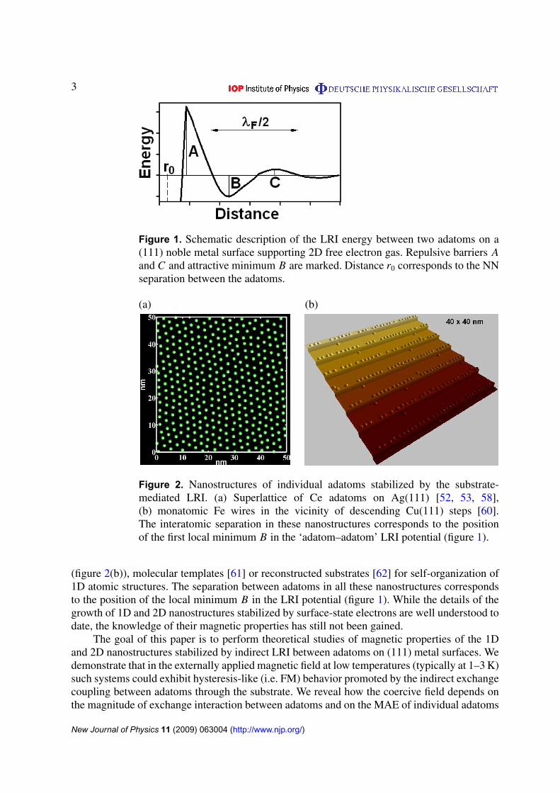
If two adatoms are separated by the first nearest neighbor (NN) distance r0 (figure 1)the interaction is determined only by the short-range chemical bonding, and it is stronglyattractive. At larger interatomic distances (>5 Å) the interplay between adatoms is causedby the elastic interaction [44, 45] and the substrate-mediated LRI. The schematic descriptionof the ‘adatom–adatom’ LRI is presented in figure 1. There is a repulsive barrier A; itsmagnitude is between 10 and 60 meV, depending on the sort of interacting adatoms and thetype of surface [41], [46]–[52]. At low temperatures (<50 K) this repulsive barrier inhibitsagglomeration of two adatoms into a dimer, decreasing the probability of cluster formation.At larger separations (see figure 1) there is an attractive minimum B; its magnitude is a fewmeV [41, 46, 47], [52]–[54]. Typically, this minimum is located at separations which are 5–10times larger than the NN distance r0. For instance, on Cu(111) the position of the minimumB is at 12 Å [41, 46, 47, 54], while on Ag(111) it is at 30 Å [52, 53]. There is yet anotherrepulsive barrier C , whose magnitude is usually less than 1 meV. According to [33], at largerseparations r , E(r) ∼ sin(α1r + α2)/r 2. The positions of the minima and maxima of the LRIpotential (figure 1) are determined by the type of surface and scattering properties of adatoms.

Several theoretical and experimental investigations have demonstrated that one can createmacroscopic-ordered 1D and 2D nanostructures exploiting atomic self-assembly promoted bysurface-state electrons. Dilute 2D nanoislands of individual adatoms stabilized by the LRI havebeen observed experimentally [46, 47] and studied theoretically [55, 56]. It has been foundthat cerium adatoms randomly deposited on Ag(111) form a perfectly ordered 2D superlattice[52, 53, 57, 58] (figure 2(a)) (for Cs on Ag(111) see [59]). One can exploit stepped surfaces [60]

New Journal of Physics 11 (2009) 063004 (http://www.njp.org/)

3

Figure 1. Schematic description of the LRI energy between two adatoms on a(111) noble metal surface supporting 2D free electron gas. Repulsive barriers Aand C and attractive minimum B are marked. Distance r0 corresponds to the NNseparation between the adatoms.

(a) (b)

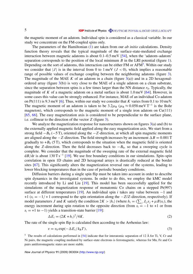
Figure 2. Nanostructures of individual adatoms stabilized by the substrate-mediated LRI. (a) Superlattice of Ce adatoms on Ag(111) [52, 53, 58],(b) monatomic Fe wires in the vicinity of descending Cu(111) steps [60].The interatomic separation in these nanostructures corresponds to the positionof the first local minimum B in the ‘adatom–adatom’ LRI potential (figure 1).

(figure 2(b)), molecular templates [61] or reconstructed substrates [62] for self-organization of1D atomic structures. The separation between adatoms in all these nanostructures correspondsto the position of the local minimum B in the LRI potential (figure 1). While the details of thegrowth of 1D and 2D nanostructures stabilized by surface-state electrons are well understood todate, the knowledge of their magnetic properties has still not been gained.

The goal of this paper is to perform theoretical studies of magnetic properties of the 1Dand 2D nanostructures stabilized by indirect LRI between adatoms on (111) metal surfaces. Wedemonstrate that in the externally applied magnetic field at low temperatures (typically at 1–3 K)such systems could exhibit hysteresis-like (i.e. FM) behavior promoted by the indirect exchangecoupling between adatoms through the substrate. We reveal how the coercive field depends onthe magnitude of exchange interaction between adatoms and on the MAE of individual adatoms

New Journal of Physics 11 (2009) 063004 (http://www.njp.org/)

4

(a) (b)

z z

Figure 3. A schematic view of two systems considered within our study:(a) finite 1D chain of equidistantly separated spins and (b) 2D hexagonal-orderedarray of equidistantly separated spins. We suppose that both systems representatomic structures stabilized by the substrate-mediated LRI (figure 2). The easymagnetization axis of an individual adatom is considered to be collinear to thevector Z . Spin orientations along and opposite to the easy axis are demonstratedusing red arrows.

within a nanostructure. We study the dependence of the magnetization response on the size ofa system (number of adatoms in a nanostructure). As a method of investigation, we employ thekinetic Monte Carlo (kMC) model for simulation of spin dynamics [19].

The remainder of the paper is organized as follows. In section 2, we give the details of themodel that was used to simulate the spin dynamics. In section 3, we present the results of ourcalculations and discuss them.

2. The model

In this section, we describe the model that was utilized to simulate spin dynamics and we discussthe parameters of the investigated systems.

Two different systems are considered. The first system is a 1D finite chain of spins(figure 3(a)), which represents a monatomic wire of magnetic adatoms stabilized by the LRI inthe vicinity of a descending step (figure 2(b)) [60] or inside a molecular trench [61]. Since theaverage distance between the wires is several times larger than the interatomic distance withina wire [60, 61], the effect of interchain exchange interaction on the magnetization responsecan be neglected. The second system under study is a 2D hexagonal-ordered array of spins(figure 3(b)), which represents magnetic adatoms assembled in a hexagonal nanoisland [46, 47]or superlattice [52, 53, 57, 58] (if the number of adatoms tends to infinity (figure 2(a))). Forboth systems the Hamiltonian of the classical Heisenberg model with an on-site anisotropy andexternal magnetic field EB can be written as [19]

H = J∑〈i, j〉

Esi Es j − K∑

i

(sz,i)2− µ EB

∑i

Esi , (1)

where Esi is the normalized spin value at site i , sz,i is the Z -component of the vector Esi (see thedirection definition in figure 3), the summation 〈i, j〉 is taken over all neighboring pairs of spinsi and j , Esi Es j is a scalar product of spins at sites i and j . J is the exchange coupling constant(J < 0 for FM and J > 0 for antiferromagnetic (AFM) interaction), K is the MAE and µ is

New Journal of Physics 11 (2009) 063004 (http://www.njp.org/)

5

the magnetic moment of an adatom. Individual spin is considered as a classical variable. In ourstudy we concentrate on the FM-coupled spins only.

The parameters of the Hamiltonian (1) are taken from our ab initio calculations. Densityfunction theory reveals that the typical magnitude of the surface-state-mediated exchangeinteraction between magnetic adatoms is about 0.1–0.5 meV [54], when the ‘adatom–adatom’separation corresponds to the position of the local minimum B in the LRI potential (figure 1).Depending on the sort of adatoms, this interaction can be either FM or AFM5. Within our studywe consider that |J | is in the interval from 0 to 1 meV (J < 0), which implies a reasonablerange of possible values of exchange coupling between the neighboring adatoms (figure 3).The magnitude of the MAE K of an adatom in a chain (figure 3(a)) and in a 2D hexagonal-ordered array (figure 3(b)) is very close to the MAE of a single adatom on a clean substrate,since the separation between spins is a few times larger than the NN distance r0. Typically, themagnitude of K of a magnetic adatom on a metal surface is about 1.0 meV [64]. However, insome cases this value can be strongly enhanced. For instance, MAE of an individual Co adatomon Pt(111) is 9.3 meV [6]. Thus, within our study we consider that K varies from 0.1 to 10 meV.The magnetic moment of an adatom is taken to be 3.2µB (µB ≈ 0.058 meV T−1 is the Bohrmagneton), which corresponds to the magnetic moment of a single iron adatom on Cu(111)[65, 66]. The easy magnetization axis is considered to be perpendicular to the surface plane,i.e. collinear to the direction of the vector Z (figure 3).

We analyze the magnetization response for nanostructures shown on figures 3(a) and (b) tothe externally applied magnetic field applied along the easy magnetization axis. We start from astrong field −B0 (−5 T), oriented along the −Z -direction, at which all spin magnetic momentsare aligned along the −Z -direction. The field strength increases by an increment 1B = 0.001 Tgradually to +B0 (5 T), which corresponds to the situation when the magnetic field is orientedalong the Z -direction. Then the field decreases back to −B0, so that a sweeping cycle iscomplete. We consider that the magnitude of the sweeping rate of the external magnetic fielddB/dt is about 130 T s−1 [19]. We use free boundary conditions in our simulations. Spin–spincorrelation in open 1D chains and 2D hexagonal arrays is drastically reduced at the bordersites [67]. This significantly alters the magnetization reversal rate of the systems, leading tolower blocking temperatures than in the case of periodic boundary conditions.

Diffusion barriers during a single spin flip must be taken into account in order to describespin dynamics in the investigated systems. In order to do this, we employ the kMC modelrecently introduced by Li and Liu [19]. This model has been successfully applied for thesimulations of the magnetization response of monatomic Co chains on a stepped Pt(997)surface at different temperatures [19]. An individual spin i takes any value between −1 and+1 (si = −1/ + 1 correspond to the spin orientation along the −Z /Z -direction, respectively). Ifmodel parameters J and K satisfy the condition 2K > |hi | (where hi = (

∑j Ji j s j + µB)si), the

energy increment during spin rotation to the opposite direction (from si = −1 to +1 or fromsi = +1 to −1) yields a transition-state barrier [19]:

1Ei = (2K + hi)2/4K . (2)

The rate of the single spin flip is calculated then according to the Arrhenius law:

v = v0 exp(−1Ei/kBT ), (3)

5 The results of calculations performed in [54] indicate that for interatomic separation of 12 Å for Ti, V, Cr andNi pairs, the magnetic coupling mediated by surface-state electrons is ferromagnetic, whereas for Mn, Fe and Copairs antiferromagnetic states are more stable.

New Journal of Physics 11 (2009) 063004 (http://www.njp.org/)

6

Figure 4. Magnetization response to the external magnetic field for the 1Dchain of N = 100 spins at two temperatures: (a) 1.0 K and (b) 2.0 K. Blackcircles correspond to the following values of parameters of the Hamiltonian (1):K = 1.0 meV, J = −0.3 meV and µ = 3.2µB, while white circles correspond to:K = 1.0 meV, J = 0 meV and µ = 3.2µB.

where kB is the Boltzmann constant and prefactor v0 is 109 Hz [10, 19]. If the condition2K 6 |hi | is satisfied, there is no transition state barrier for the spin reversal process, and theGlauber method [68] is used to compute the exponential factor of the rates, with the prefactorto be the same.

If the total number of spins in a system is equal to N , then for every kMC step N differentspin flips with the rates v1, v2, . . . , vN are possible. The time increment τ corresponding to onestep of the kMC algorithm is computed using the formulae [63]:

τ = −ln U/ N∑

i=1

νi , (4)

where U is a randomly distributed number in the interval (0, 1).

3. Results and discussion

We start this section with the investigation of the magnetization response for a 1D chain of spins(figure 3(a)).

Figure 4 demonstrates the magnetization response for a chain (figure 3(a)) consisting ofN = 100 spins at two temperatures: 1.0 K (figure 4(a), black circles) and 2.0 K (figure 4(b),black circles). During simulations we have considered that J = −0.3 meV and K = 1.0 meV.At the lower temperature the system exhibits hysteresis-like (FM) behavior, while at the highertemperature no hysteresis loop is observed. The hysteresis loop is characterized by the criticalmagnetic field Bc at which the magnetization is zero. The magnitude of coercive field Bc atT = 1.0 K is 0.26 T. While the exchange coupling constant between spins is relatively small(J = −0.3 meV), the exchange interaction is the dominant factor responsible for the observed

New Journal of Physics 11 (2009) 063004 (http://www.njp.org/)

7

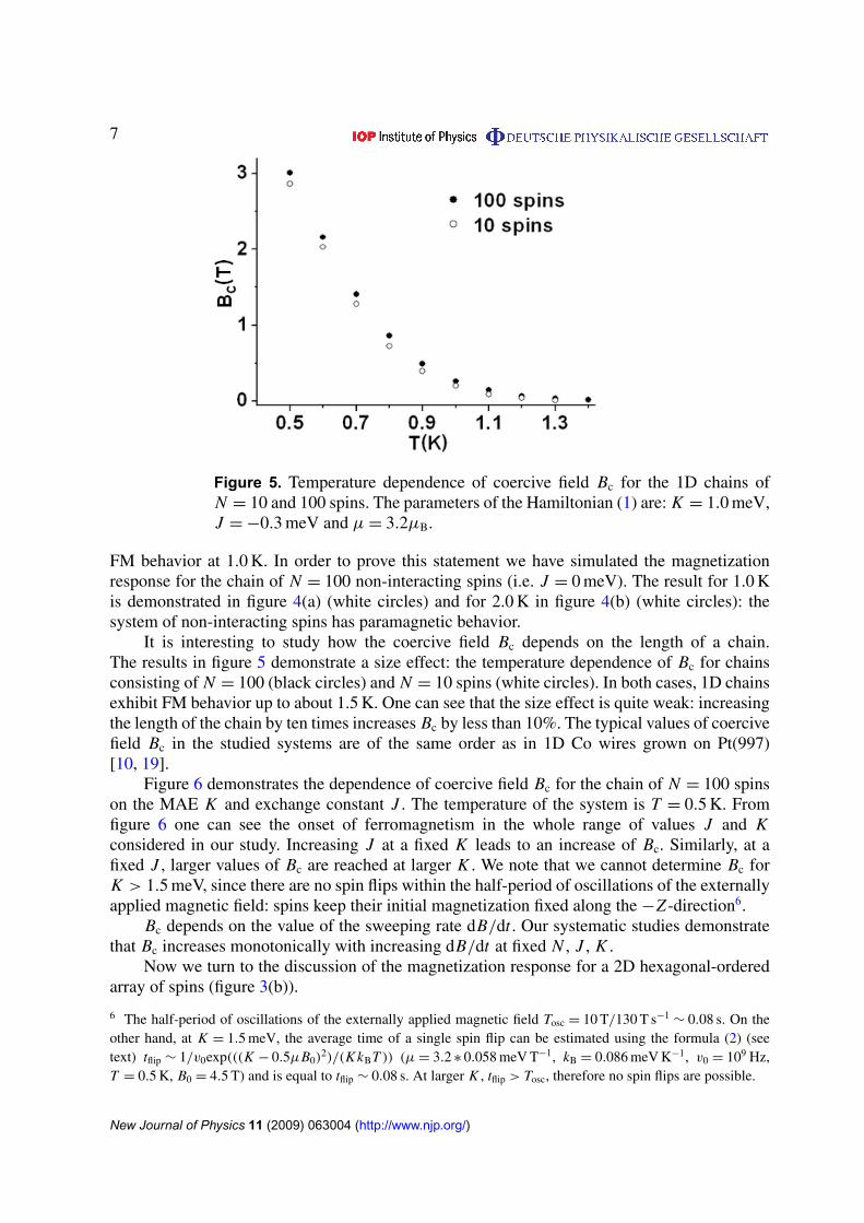
Figure 5. Temperature dependence of coercive field Bc for the 1D chains ofN = 10 and 100 spins. The parameters of the Hamiltonian (1) are: K = 1.0 meV,J = −0.3 meV and µ = 3.2µB.

FM behavior at 1.0 K. In order to prove this statement we have simulated the magnetizationresponse for the chain of N = 100 non-interacting spins (i.e. J = 0 meV). The result for 1.0 Kis demonstrated in figure 4(a) (white circles) and for 2.0 K in figure 4(b) (white circles): thesystem of non-interacting spins has paramagnetic behavior.

It is interesting to study how the coercive field Bc depends on the length of a chain.The results in figure 5 demonstrate a size effect: the temperature dependence of Bc for chainsconsisting of N = 100 (black circles) and N = 10 spins (white circles). In both cases, 1D chainsexhibit FM behavior up to about 1.5 K. One can see that the size effect is quite weak: increasingthe length of the chain by ten times increases Bc by less than 10%. The typical values of coercivefield Bc in the studied systems are of the same order as in 1D Co wires grown on Pt(997)[10, 19].

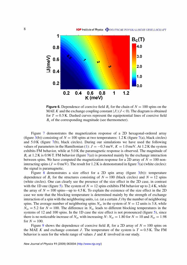
Figure 6 demonstrates the dependence of coercive field Bc for the chain of N = 100 spinson the MAE K and exchange constant J . The temperature of the system is T = 0.5 K. Fromfigure 6 one can see the onset of ferromagnetism in the whole range of values J and Kconsidered in our study. Increasing J at a fixed K leads to an increase of Bc. Similarly, at afixed J , larger values of Bc are reached at larger K . We note that we cannot determine Bc forK > 1.5 meV, since there are no spin flips within the half-period of oscillations of the externallyapplied magnetic field: spins keep their initial magnetization fixed along the −Z -direction6.

Bc depends on the value of the sweeping rate dB/dt . Our systematic studies demonstratethat Bc increases monotonically with increasing dB/dt at fixed N , J , K .

Now we turn to the discussion of the magnetization response for a 2D hexagonal-orderedarray of spins (figure 3(b)).

6 The half-period of oscillations of the externally applied magnetic field Tosc = 10 T/130 T s−1∼ 0.08 s. On the

other hand, at K = 1.5 meV, the average time of a single spin flip can be estimated using the formula (2) (seetext) tflip ∼ 1/v0exp(((K − 0.5µB0)

2)/(K kBT )) (µ = 3.2 ∗ 0.058 meV T−1, kB = 0.086 meV K−1, v0 = 109 Hz,T = 0.5 K, B0 = 4.5 T) and is equal to tflip ∼ 0.08 s. At larger K , tflip > Tosc, therefore no spin flips are possible.

New Journal of Physics 11 (2009) 063004 (http://www.njp.org/)

8

Figure 6. Dependence of coercive field Bc for the chain of N = 100 spins on theMAE K and the exchange coupling constant |J | (J < 0). The diagram is obtainedfor T = 0.5 K. Dashed curves represent the equipotential lines of coercive fieldBc of the corresponding magnitude (see thermometer).

Figure 7 demonstrates the magnetization response of a 2D hexagonal-ordered array(figure 3(b)) consisting of N = 100 spins at two temperatures: 1.2 K (figure 7(a), black circles)and 5.0 K (figure 7(b), black circles). During our simulations we have used the followingvalues of parameters in the Hamiltonian (1): J = −0.3 meV, K = 1.0 meV. At 1.2 K the systemexhibits FM behavior, while at 5.0 K the paramagnetic response is observed. The magnitude ofBc at 1.2 K is 0.96 T. FM behavior (figure 7(a)) is promoted mainly by the exchange interactionbetween spins. We have computed the magnetization response for a 2D array of N = 100 non-interacting spins (J = 0 meV). The result for 1.2 K is demonstrated in figure 7(a) (white circles):the signal is paramagnetic.

Figure 8 demonstrates a size effect for a 2D spin array (figure 3(b)): temperaturedependence of Bc for the structures consisting of N = 100 (black circles) and N = 12 spins(white circles). One can clearly see the presence of the size effect in the 2D case, in contrastwith the 1D one (figure 5). The system of N = 12 spins exhibits FM behavior up to 2.4 K, whilethe array of N = 100 spins—up to 4.5 K. To explain the existence of the size effect in the 2Dcase we note that the blocking temperature is determined mainly by the strength of exchangeinteraction of a spin with the neighboring units, i.e. (at a certain J ) by the number of neighboringspins. The average number of neighboring spins Nav in the system of N = 12 units is 3.8, whileNav = 5.2 for N = 100. The difference in Nav leads to different blocking temperatures in thesystems of 12 and 100 spins. In the 1D case the size effect is not pronounced (figure 5), sincethere is no noticeable increase of Nav with increasing N : Nav = 1.80 for N = 10 and Nav = 1.98for N = 100.

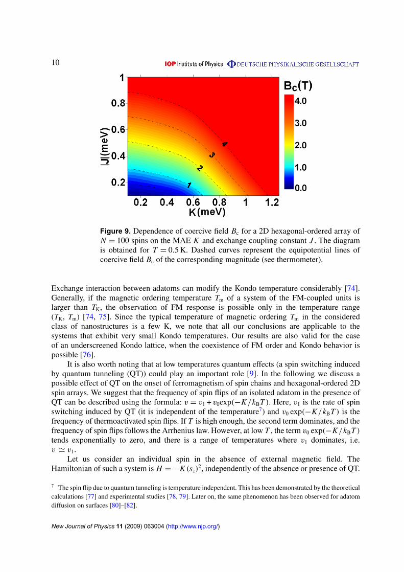
Figure 9 shows the dependence of coercive field Bc for a 2D array of N = 100 spins onthe MAE K and exchange constant J . The temperature of the system is T = 0.5 K. The FMbehavior is seen for the whole range of values J and K involved in our study.

New Journal of Physics 11 (2009) 063004 (http://www.njp.org/)

9

Figure 7. Magnetization response to the external magnetic field for the 2Dhexagonal-ordered array of N = 100 spins at two temperatures: (a) 1.2 K,(b) 5.0 K. Black circles correspond to the following parameters of theHamiltonian (1): K = 1.0 meV, J = −0.3 meV and µ = 3.2µB, while whitecircles correspond to: K = 1.0 meV, J = 0 meV and µ = 3.2µB.

Figure 8. Temperature dependence of coercive field Bc for 2D hexagonal-ordered arrays of N = 12 and 100 spins. The parameters of the Hamiltonian (1)are: K = 1.0 meV, J = −0.3 meV and µ = 3.2µB.

It is of great importance to discuss the Kondo effect [69]–[73], which could arise in theconsidered class of the 1D and 2D systems (figure 2). In the Kondo effect, a localized magneticmoment of an adatom is screened below the Kondo temperature TK and forms a correlatedelectron system with the surrounding conduction electrons on the non-magnetic host [69]–[73].

New Journal of Physics 11 (2009) 063004 (http://www.njp.org/)

10

Figure 9. Dependence of coercive field Bc for a 2D hexagonal-ordered array ofN = 100 spins on the MAE K and exchange coupling constant J . The diagramis obtained for T = 0.5 K. Dashed curves represent the equipotential lines ofcoercive field Bc of the corresponding magnitude (see thermometer).

Exchange interaction between adatoms can modify the Kondo temperature considerably [74].Generally, if the magnetic ordering temperature Tm of a system of the FM-coupled units islarger than TK, the observation of FM response is possible only in the temperature range(TK, Tm) [74, 75]. Since the typical temperature of magnetic ordering Tm in the consideredclass of nanostructures is a few K, we note that all our conclusions are applicable to thesystems that exhibit very small Kondo temperatures. Our results are also valid for the caseof an underscreened Kondo lattice, when the coexistence of FM order and Kondo behavior ispossible [76].

It is also worth noting that at low temperatures quantum effects (a spin switching inducedby quantum tunneling (QT)) could play an important role [9]. In the following we discuss apossible effect of QT on the onset of ferromagnetism of spin chains and hexagonal-ordered 2Dspin arrays. We suggest that the frequency of spin flips of an isolated adatom in the presence ofQT can be described using the formula: v = v1 + v0exp(−K/kBT ). Here, v1 is the rate of spinswitching induced by QT (it is independent of the temperature7) and v0 exp(−K/kBT ) is thefrequency of thermoactivated spin flips. If T is high enough, the second term dominates, and thefrequency of spin flips follows the Arrhenius law. However, at low T , the term v0 exp(−K/kBT )

tends exponentially to zero, and there is a range of temperatures where v1 dominates, i.e.v ' v1.

Let us consider an individual spin in the absence of external magnetic field. TheHamiltonian of such a system is H = −K (sz)

2, independently of the absence or presence of QT.

7 The spin flip due to quantum tunneling is temperature independent. This has been demonstrated by the theoreticalcalculations [77] and experimental studies [78, 79]. Later on, the same phenomenon has been observed for adatomdiffusion on surfaces [80]–[82].

New Journal of Physics 11 (2009) 063004 (http://www.njp.org/)

11

Figure 10. Magnetization response for a single Co adatom on Pt(111) at 0.3and 4.2 K. The following parameters are used for simulations: v1 = 104 Hz,K = 9.3 meV, µ = 3.8µB, B0 = 7.5 T and dB/dt = 0.01 T s−1.

The activation barrier K derived from this Hamiltonian sets the switching rate in the absence ofQT: v = v0 exp(−K/kBT ). The frequency of spin flips in the presence of QT can be written inthe similar form: v = [v1exp(K/kBT ) + v0]exp(−K/kBT ). Since the Hamiltonian in both casesis the same, one can consider

veff = v0 + v1 exp(K/kBT ) (5)

as a new ‘effective’ prefactor instead of v0 (see equation (3)) for the calculation of switchingrate in the presence of QT in the framework of the applied kMC algorithm [19].

Let us now discuss possible values of v1. The upper limit of v1 is set by the condition v1 �

v0, which is derived from the fact that at high T (T → ∞) the frequency of thermoactivated spinflips v0 is much larger than the frequency of spin flips promoted by QT. Therefore, v1 � 109 Hz.The rough estimation of the lower limit of v1 can be obtained from the experimental studies ofMeier et al [9] on the magnetization response of individual Co adatoms placed on a Pt(111)surface. The S-like paramagnetic curves over Co adatoms on Pt(111) have been recorded attwo different temperatures, 0.3 and 4.2 K [9]. It is well known that a Co adatom on Pt(111) hasMAE K = 9.3 meV [6, 9]. From the formula 1/tav ∼ v0exp(−K/kBT ) (where tav is the averagetime of a thermoactivated spin flip), one finds that tav = 10147 s at T = 0.3 K and tav = 102 s atT = 4.2 K. At the same time, Meier et al [9] have reported that spin switching takes place muchfaster than the resolution time of the experiment (100 Hz). Hence the observed value of tav is�0.01 s. It has been suggested that either QT or current-induced magnetization switching couldpromote ‘fast’ spin flips of individual Co adatoms [9]. If we suggest that QT is responsible forthe observed spin switching, we obtain the lower limit of v1 � 102 Hz. As a result, we concludethat most probably v1 is in the range between 104 and 107 Hz.

In order to take into account quantum effects, we have modified the kMC model describedin section 2. The procedure of calculation of activation barriers remains unchanged; however,

New Journal of Physics 11 (2009) 063004 (http://www.njp.org/)

12

Figure 11. Effect of QT on the magnetization response for the 1D chain ofN = 100 spins at T = 1.0 K. Black circles correspond to v1 = 0 (absence ofQT), white circles to v1 = 104 Hz, blue circles to v1 = 105 Hz and red circles tov1 = 106 Hz. The values of the parameters of the Hamiltonian (1): K = 1.0 meV,J = −0.3 meV and µ = 3.2µB.

we employ prefactor veff (see equation (5)) instead of v0 to compute transition rates (seeequation (3)). To illustrate the concept of veff, firstly we have followed the experimental setup ofMeier et al [9] on the magnetization response of individual Co adatoms on Pt(111) at thetemperatures 0.3 and 4.2 K. The following values of parameters have been used in ourcalculations: K = 9.3 meV, µ = 3.8µB, B0 = 7.5 T and dB/dt = 0.01 T s−1 (slow sweepingrate). The results of kMC simulations are presented in figure 10. For the calculations we haveconsidered that v1 = 104 Hz. We have also tested other magnitudes of v1 within the rangefrom 104 to 107 Hz and we have found that both the resulting curves remain unchanged. Fromfigure 10 one can see that the magnetization response at both temperatures is paramagnetic. Thevalues of saturation fields are about 0.3 T at 0.3 K and about 5.0 T at 4.2 K, in agreement withthe experimental observations [9].

We now turn to the effect of QT on the possible onset of ferromagnetism in 1D spinchains and 2D hexagonal-ordered spin arrays at low temperatures. Figure 11 demonstrates themagnetization response for a chain of N = 100 spins at T = 1.0 K. We have already found(figure 4(a)) that this system exhibits FM behavior with coercive field Bc = 0.26 T (black circlesin figure 11). White circles represent the magnetic signal calculated at v1 = 104 Hz: FM responsewith Bc = 0.18 T. In the case of v1 = 105 Hz (blue circles), we find that Bc = 0.07 T. Red circlesdemonstrate the magnetization response at v1 = 106 Hz: hysteresis loop with Bc = 0.02 T isobserved. If v1 = 107 Hz, then Bc = 0.003 T (not shown in figure 11). Taking into account theresults shown in figure 11, we conclude that QT could decrease the coercive field Bc. However,it does not influence the onset of ferromagnetism in 1D spin arrays.

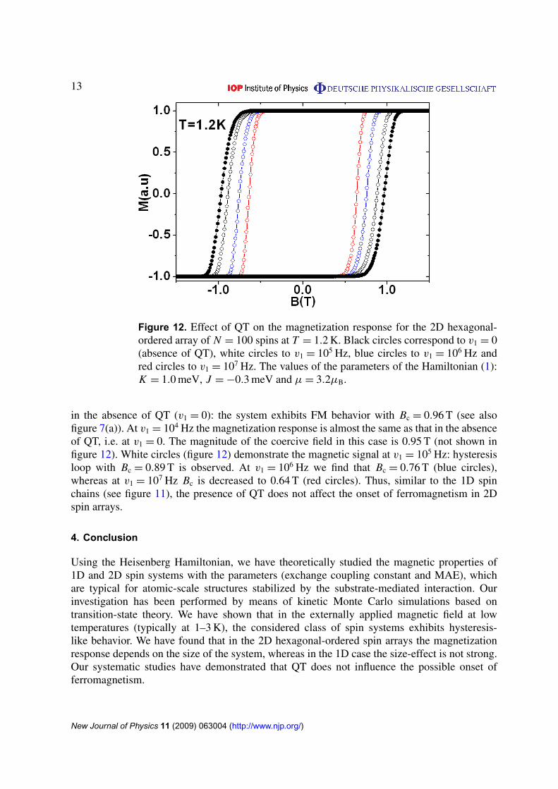
We have also investigated the effect of QT on the magnetic behavior of the 2D array ofN = 100 spins at T = 1.2 K (figure 12). Black circles demonstrate the hysteresis loop obtained

New Journal of Physics 11 (2009) 063004 (http://www.njp.org/)

13

Figure 12. Effect of QT on the magnetization response for the 2D hexagonal-ordered array of N = 100 spins at T = 1.2 K. Black circles correspond to v1 = 0(absence of QT), white circles to v1 = 105 Hz, blue circles to v1 = 106 Hz andred circles to v1 = 107 Hz. The values of the parameters of the Hamiltonian (1):K = 1.0 meV, J = −0.3 meV and µ = 3.2µB.

in the absence of QT (v1 = 0): the system exhibits FM behavior with Bc = 0.96 T (see alsofigure 7(a)). At v1 = 104 Hz the magnetization response is almost the same as that in the absenceof QT, i.e. at v1 = 0. The magnitude of the coercive field in this case is 0.95 T (not shown infigure 12). White circles (figure 12) demonstrate the magnetic signal at v1 = 105 Hz: hysteresisloop with Bc = 0.89 T is observed. At v1 = 106 Hz we find that Bc = 0.76 T (blue circles),whereas at v1 = 107 Hz Bc is decreased to 0.64 T (red circles). Thus, similar to the 1D spinchains (see figure 11), the presence of QT does not affect the onset of ferromagnetism in 2Dspin arrays.

4. Conclusion

Using the Heisenberg Hamiltonian, we have theoretically studied the magnetic properties of1D and 2D spin systems with the parameters (exchange coupling constant and MAE), whichare typical for atomic-scale structures stabilized by the substrate-mediated interaction. Ourinvestigation has been performed by means of kinetic Monte Carlo simulations based ontransition-state theory. We have shown that in the externally applied magnetic field at lowtemperatures (typically at 1–3 K), the considered class of spin systems exhibits hysteresis-like behavior. We have found that in the 2D hexagonal-ordered spin arrays the magnetizationresponse depends on the size of the system, whereas in the 1D case the size-effect is not strong.Our systematic studies have demonstrated that QT does not influence the possible onset offerromagnetism.

New Journal of Physics 11 (2009) 063004 (http://www.njp.org/)

14

Acknowledgments

We thank L M Sandratskii (MPI-Halle) for stimulating discussions. This work was supportedby the Deutsche Forschungsgemeinschaft (SPP1165 and SPP1153).

References

[1] Barth J V, Costantini G and Kern K 2005 Nature 437 671[2] Himspel F J, Ortega J E, Mankey G J and Willis R F 1998 Adv. Phys. 47 511[3] Lu C L, Freeman A J and Oguchi T 1985 Phys. Rev. Lett. 54 2700[4] Stepanyuk V S, Hergert W, Wildberger K, Zeller R and Dederichs P H 1996 Phys. Rev. B 53 2121[5] Nonas B, Cabria I, Zeller R, Dederichs P H, Huhne T and Ebert H 2001 Phys. Rev. Lett. 86 2146[6] Gambardella P et al 2003 Science 300 1130[7] Gambardella P, Rusponi S, Cren T, Weiss N and Brune H 2005 C. R. Phys. 6 75[8] Hirjibehedin C F, Lin C-Y, Otte A F, Ternes M, Lutz C P, Jones B A and Heinrich A J 2007 Science 317

1199[9] Meier F, Zhou L, Wiebe J and Wiesendanger R 2008 Science 320 82

[10] Gambardella P, Dallmeyer A, Maiti K, Malagoli M C, Eberhardt W, Kern K and Carbone C 2002 Nature 416301

[11] Shen J, Pierce J P, Plummer E W and Kirschner J 2003 J. Phys.: Condens. Matter 15 R1[12] Hillenkamp M, Di Domenicantonio G and Félix C 2008 Phys. Rev. B 77 014422[13] Elmers H J, Hauschild J, Höche H, Gradmann U, Bethge H, Heuer D and Köhler U 1994 Phys. Rev. Lett. 73

898[14] Shen J, Skomski R, Klaua M, Jenniches H, Manoharan S S and Kirschner J 1997 Phys. Rev. B 56 2340[15] Brown G, Lee H K, Schulthess T C, Ujfalussy B, Stocks G M, Butler W H, Landau D P, Pierce J P, Shen J

and Kirschner J 2002 J. Appl. Phys. 91 7056[16] Yan L, Przybylski M, Lu Y F, Wang W H, Barthel J and Kirschner J 2005 Appl. Phys. Lett. 86 102503[17] Shiraki S, Fujisawa H, Nakamura T, Muro T, Nantoh M and Kawai M 2008 Phys. Rev. B 78 115428[18] Gambardella P 2003 J. Phys.: Condens. Matter 15 2533[19] Li Y and Liu B-G 2006 Phys. Rev. B 73 174418[20] Dorantes-Dávila J and Pastor G M 1998 Phys. Rev. Lett. 81 208[21] Spisak D and Hafner J 2002 Phys. Rev. B 65 235405[22] Fruchart O, Klaua M, Barthel J and Kirschner J 1999 Phys. Rev. Lett. 83 2769[23] Qiang Y, Sabiryanov R F, Jaswal S S, Liu Y, Haberland H and Sellmyer D J 2002 Phys. Rev. B 66 064404[24] Pierce J P, Torija M A, Gai Z, Shi J, Schulthess T C, Farnan G A, Wendelken J F, Plummer E W and Shen J

2004 Phys. Rev. Lett. 92 237201[25] Torija M A, Li A P, Guan X C, Plummer E W and Shen J 2005 Phys. Rev. Lett. 93 257203[26] Rohart S, Repain V, Tejeda A, Ohresser P, Scheurer F, Bencok P, Ferrer J and Rousset S 2006 Phys. Rev. B

73 165412[27] Skomski R, Zhang J, Sessi V, Honolka J, Enders A and Kern K 2008 J. Appl. Phys. 103 07D519[28] Poulopoulos P, Jensen P J, Ney A, Lindner J and Baberschke K 2002 Phys. Rev. B 65 064431[29] Hernando A, Briones F, Cebollada A and Crespo P 2002 Physica B 322 318[30] Zhou J, Skomski R and Sellmyer D J 2006 J. Appl. Phys. 99 08F909[31] Einstein T L and Schrieffer J R 1973 Phys. Rev. B 7 3629[32] Lau K H and Kohn W 1978 Surf. Sci. 75 69[33] Hyldgaard P and Persson M 2000 J. Phys.: Condens. Matter. 12 L13[34] Brune H, Wintterlin J, Ertl G and Behm R J 1990 Europhys. Lett. 13 123[35] Crommie M F, Lutz C P and Eigler D M 1993 Science 262 218[36] Crommie M F, Lutz C P and Eigler D M 1993 Nature 363 524

New Journal of Physics 11 (2009) 063004 (http://www.njp.org/)

15

[37] Li J, Schneider W-D, Berndt R and Crampin S 1998 Phys. Rev. Lett. 80 3332[38] Bürgi L, Jeandupeux O, Hirstein A, Brune H and Kern K 1998 Phys. Rev. Lett. 81 5370[39] Braun K-F and Rieder K-H 2002 Phys. Rev. Lett. 88 096801[40] Pivetta M, Silly F, Patthey F, Pelz J P and Schneider W-D 2003 Phys. Rev. B 67 193402[41] Stepanyuk V S, Baranov A N, Tsivlin D V, Hergert W, Bruno P, Knorr N, Schneider M A and Kern K 2003

Phys. Rev. B 68 205410[42] Negulyaev N N, Stepanyuk V S, Niebergall L, Bruno P, Hergert W, Repp J, Rieder K-H and Meyer G 2008

Phys. Rev. Lett. 101 226601[43] Bürgi L, Knorr N, Brune H, Schneider M A and Kern K 2002 Appl. Phys. A 75 141[44] Lau K H and Kohn W 1977 Surf. Sci. 65 607[45] Longo R C, Stepanyuk V S and Kirschner J 2006 J. Phys.: Condens. Matter 18 9143[46] Repp J, Moresco F, Meyer G, Rieder K-H, Hyldgaard P and Persson M 2000 Phys. Rev. Lett. 85 2981[47] Knorr N, Brune H, Epple M, Hirstein A, Schneider M A and Kern K 2002 Phys. Rev. B 65 115420[48] Bogicevic A, Ovesson S, Hyldgaard P, Lundqvist B I, Brune H and Jennison D R 2000 Phys. Rev. Lett. 85

1910[49] Fichthorn K A and Scheffler M 2000 Phys. Rev. Lett. 84 5371[50] Fichthorn K A, Merrick M L and Scheffler M 2002 Appl. Phys. A 75 17[51] Fichthorn K A, Merrick M L and Scheffler M 2003 Phys. Rev. B 68 041404[52] Silly F, Pivetta M, Ternes M, Patthey F, Pelz J P and Schneider W-D 2004 New J. Phys. 6 16[53] Silly F, Pivetta M, Ternes M, Patthey F, Pelz J P and Schneider W-D 2004 Phys. Rev. Lett. 92 016101[54] Stepanyuk V S, Niebergall L, Longo R C, Hergert W and Bruno P 2004 Phys. Rev. B 70 075414[55] Rogowska J M and Maciejewski M 2006 Phys. Rev. B 74 235402[56] Hu J, Teng B, Wu F and Fang Y 2008 New J. Phys. 10 023033[57] Ternes M, Weber C, Pivetta M, Patthey F, Pelz J P, Giamarchi T, Mila F and Schneider W-D 2004 Phys. Rev.

Lett. 93 146805[58] Negulyaev N N, Stepanyuk V S, Niebergall L, Hergert W, Fangohr H and Bruno P 2006 Phys. Rev. B 74

035421[59] Ziegler M, Kröger J, Berndt R, Filinov A and Bonitz M 2008 Phys. Rev. B 78 245427[60] Ding H F, Stepanyuk V S, Ignatiev P A, Negulyaev N N, Niebergall L, Wasniowska M, Gao C L, Bruno P

and Kirschner J 2007 Phys. Rev. B 76 033409[61] Schiffrin A, Reichert J, Auwärter W, Jahnz G, Pennec Y, Weber-Bargioni A, Stepanyuk V S, Niebergall L,

Bruno P and Barth J V 2008 Phys. Rev. B 78 035424[62] Liu C, Uchihashi T and Nakayama T 2008 Phys. Rev. Lett. 101 146104[63] Fichthorn K A and Weinberg W H 1991 J. Chem. Phys. 95 1090[64] Pick S, Stepanyuk V S, Klavsyuk A L, Niebergall L, Hergert W, Kirschner J and Bruno P 2004 Phys. Rev. B

70 224419[65] Lazarovits B, Szunyogh L and Weinberger P 2006 Phys. Rev. B 73 045430[66] Lounis S, Mavropoulos P, Dederichs P H and Blügel S 2006 Phys. Rev. B 73 195421[67] Vindigni A, Rettori A, Pini M G, Carbone C and Gambardella P 2006 Appl. Phys. A 82 385[68] Glauber R J 1963 J. Math. Phys. 4 294[69] Li J, Schneider W-D, Berndt R and Delley B 1998 Phys. Rev. Lett. 80 2893[70] Madhavan V, Chen W, Jamneala T, Crommie M F and Wingreen N S 1998 Science 280 567[71] Wahl P, Diekhöner L, Schneider M A, Vitali L, Wittich G and Kern K 2004 Phys. Rev. Lett. 93 176603[72] Otte A F, Ternes M, von Bergmann K, Loth S, Brune H, Lutz C P, Hirjibehedin C F and Heinrich A J 2008

Nat. Phys. 4 847[73] Ternes M, Heinrich A J and Schneider W-D 2009 J. Phys.: Condens. Matter 21 053001[74] Wahl P, Simon P, Diekhöner L, Stepanyuk V S, Bruno P, Schneider M A and Kern K 2007 Phys. Rev. Lett. 98

056601

New Journal of Physics 11 (2009) 063004 (http://www.njp.org/)

16

[75] Lee W H, Shelton R N, Dhar S K and Gschneider K A 1987 Phys. Rev. B 35 8523[76] Perkins N B, Iglesias J R, Núñez-Regueiro M D and Coqblin B 2007 Europhys. Lett. 79 57006[77] Chudnovsky E M and Gunther L 1988 Phys. Rev. Lett. 60 661[78] Friedman J R, Sarachik M P, Tejada J and Ziolo R 1996 Phys. Rev. Lett. 76 3830[79] Thomas L, Lionti F, Ballou R, Gatteschi D, Sessoli R and Barbara B 1996 Nature 383 145[80] Lauhon L J and Ho W 2000 Phys. Rev. Lett. 85 4566[81] Repp J, Meyer G, Rieder K-H and Hyldgaard P 2003 Phys. Rev. Lett. 91 206102[82] Gadzuk J W 2006 Phys. Rev. B 73 085401

New Journal of Physics 11 (2009) 063004 (http://www.njp.org/)