T h e o p e n – a c c e s s j o u r n a l f o r p h y s i c s

New Journal of Physics

Optimal signal states for quantum detectors

Ognyan Oreshkov1,2,5, John Calsamiglia1, Ramon Muñoz-Tapia1

and Emili Bagan1,3,4

1 Física Teòrica: Informació i Fenòmens Quàntics, Universitat Autònoma deBarcelona, 08193 Bellaterra (Barcelona), Spain2 QuIC, Ecole Polytechnique, CP 165, Université Libre de Bruxelles,1050 Brussels, Belgium3 Department of Physics, Hunter College of the City University of New York,695 Park Avenue, New York, NY 10021, USA4 HET Group, Physics Department, Brookhaven National Laboratory, Upton,NY 11973, USAE-mail: oreshkov@ulb.ac.be

New Journal of Physics 13 (2011) 073032 (22pp)Received 4 April 2011Published 22 July 2011Online at http://www.njp.org/doi:10.1088/1367-2630/13/7/073032

Abstract. Quantum detectors provide information about the microscopicproperties of quantum systems by establishing correlations between thoseproperties and a set of macroscopically distinct events that we observe. Thequestion of how much information a quantum detector can extract from a systemis therefore of fundamental significance. In this paper, we address this questionwithin a precise framework: given a measurement apparatus implementing aspecific POVM measurement, what is the optimal performance achievable withit for a specific information readout task and what is the optimal way to encodeinformation in the quantum system in order to achieve this performance? Weconsider some of the most common information transmission tasks—the Bayescost problem, unambiguous message discrimination and the maximal mutualinformation. We provide general solutions to the Bayesian and unambiguousdiscrimination problems. We also show that the maximal mutual informationis equal to the classical capacity of the quantum-to-classical channel describingthe measurement, and study its properties in certain special cases. For a groupcovariant measurement, we show that the problem is equivalent to the problemof accessible information of a group covariant ensemble of states. We giveanalytical proofs of optimality in some relevant cases. The framework presented

5 Author to whom any correspondence should be addressed.

New Journal of Physics 13 (2011) 0730321367-2630/11/073032+22$33.00 © IOP Publishing Ltd and Deutsche Physikalische Gesellschaft

2

here provides a natural way to characterize generalized quantum measurementsin terms of their information readout capabilities.

Contents

1. Introduction 22. The Bayes cost problem 33. Unambiguous message discrimination 64. Mutual information 85. Example: the symmetric informationally complete positive operator-valued

measure on a qubit 155.1. Minimum error discrimination . . . . . . . . . . . . . . . . . . . . . . . . . . 155.2. Unambiguous discrimination . . . . . . . . . . . . . . . . . . . . . . . . . . . 175.3. Mutual information . . . . . . . . . . . . . . . . . . . . . . . . . . . . . . . . 18

6. Conclusion 20Acknowledgments 21References 21

1. Introduction

Quantum detectors provide the interface between the microscopic world of quantum phenomenaand the world of macroscopically distinct events that we observe. A quantum detector is a devicethat interacts with the system under observation in a way that establishes correlations betweencertain properties of the system and a set of macroscopically distinct (orthogonal) states of thedevice. A general quantum detector can be described by a positive operator-valued measure(POVM), i.e. a set of positive operators {Ei}, Ei > 0, i = 1, . . . ,M , summing up to the identity,∑

i Ei = I . For an input state ρ, the probability that the measurement yields outcome j is givenby the Born rule, p j(ρ)= Tr{ρE j}.

A natural question is: To what extent is a given quantum detector able to provideinformation about the system it is used to observe? This question can be conveniently formulatedin the context of a quantum communication scenario, where a sender (Alice) tries to sendmessages to a receiver (Bob) who is constrained to read those messages using the quantumdetector in question. Concretely, let the source of classical information that Alice wantsto communicate to Bob be characterized by a probability distribution πi > 0, i = 1, . . . , N ,∑

i πi = 1, which specifies the probability of each classical message i . Alice encodes thedifferent messages into quantum states via an encoding map i → ρi , and Bob reads theinformation by carrying out the POVM measurement. If there are no constraints on the wayAlice can prepare the signal states and these states can reach Bob undisturbed (i.e. Alice andBob are connected through a noiseless channel), then the optimal performance they can achievefor a given task can be regarded as quantifying the readout capabilities of the measurementwith respect to that task. In this respect, a problem of primary importance is to find the optimalencoding (or signal states ρi ) for which the detector achieves its optimal performance.

The problem just outlined bears strong similarities to the problem of quantum statediscrimination [1–8], where the encoding of Alice is fixed and Bob’s task is to decide whichmessage he has received by optimizing his measurement. In fact, we will see below that the two

New Journal of Physics 13 (2011) 073032 (http://www.njp.org/)

3

problems can be regarded as dual to each other due to the symmetry that exists between theinput ensembles and the POVM measurements. This allows one to adopt results from quantumstate discrimination to the problem at hand. However, since in quantum state discrimination thespace over which we optimize is more constrained due to the completeness relation

∑i Ei = I ,

it turns out that in many cases the problem of optimal signal states for quantum detectors iseasier to solve.

In addition to its application in characterizing detectors, the problem considered here is ofnatural practical interest for quantum communication, since generating different signal states [9]can be experimentally more accessible than carrying out different measurements. A quantumdetector is usually fixed, while a preparation device, although possibly also based on a fixed(but nondestructive!) measurement, can be used together with post-selection, which providesadditional flexibility to the preparation process. Furthermore, in the case of communicationthrough a noiseless channel, any operation at the receiver’s side prior to the detector can beequally done as part of the preparation strategy.

In this paper, we consider the above problem from the perspective of three differentinformation transmission tasks—the task of optimal Bayes cost message discrimination(of which the well-known problem of minimum error discrimination is a special case),unambiguous message discrimination and the maximal mutual information. Due to thesimplification mentioned above, we are able to provide solutions to the Bayesian andunambiguous discrimination problems in the general case. For the maximal mutual information,we show that this quantity is equal to the classical capacity of the quantum-to-classicalchannel corresponding to the measurement, which we term the ‘capacity of the measurement’.This quantity provides a general figure of merit for the information readout capabilities of adetector. Based on its relation to the accessible information [6], we prove a result similar toDavies’s theorem [2] (proposition 2), which shows that the optimal ensemble can be chosento consist of d2 pure states, where d is the dimension of the system. For a group covariantmeasurement, we find that the problem is equivalent to that of accessible information of agroup covariant ensemble of states. We apply our results to the case of a noisy two-levelsymmetric informationally complete measurement, for whose capacity we give analytical proofsof optimality.

2. The Bayes cost problem

In the Bayes cost problem, one is interested in minimizing an average cost function of the form

C(P)=

∑i j

Ci j Pi j , (1)

where Pi j = Tr(πiρi E j) are the joint probabilities for input i and measurement outcome j ,and Ci j > 0 are the elements of the cost matrix (Ci j is the cost of choosing hypothesis j whenhypothesis i is true). In what we will refer to as the straight version of this problem, one assumesthat the encoding i → ρi is given, and the task is to find the measurement {E j} that minimizesthe quantity in equation (1) [1]. An example of a Bayes cost problem is that of minimum errordiscrimination, i.e. minimizing the probability for incorrectly identifying the message. In thiscase, the probability for an error is given by perr =

∑i 6= j Pi j , i.e. the elements of the cost matrix

are Ci j = 1 − δi j .Here, we are concerned with the opposite scenario, which we will refer to as the reverse

problem: we assume that the receiver has an apparatus that implements a particular POVM

New Journal of Physics 13 (2011) 073032 (http://www.njp.org/)

4

measurement, and we ask what is the optimal way to encode the classical messages into quantumstates so that, using only the given POVM measurement and possibly some side informationprocessing, the receiver will identify the message at the lowest cost6. This side informationprocessing involves finding the optimal way of choosing hypothesis i when the measurementoutcome k takes place and includes the possibility of following a mixed strategy, i.e. assigninga hypothesis i randomly according to some prescribed probability distribution, which might ofcourse depend on the outcome k. In other words, the receiver can use the given POVM {Ek} toobtain new POVM measurements with elements of the form

E j =

∑k

p( j |k)Ek,∑

j

p( j |k)= 1 for all k, (2)

where 06 p( j |k)6 1 are conditional probabilities.Up to a renormalization of the cost matrix, we can assume that 06 Ci j 6 1. Hence, the

problem is equivalent to that of maximizing the quantity

B(P)≡ 1 − C(P)=

∑i j

(1 − Ci j)Pi j ≡

∑i j

Bi j Pi j , (3)

where

06 Bi j 6 1, ∀i, j. (4)

For a given POVM measurement {Ei}, consider some encoding and decoding strategiesgiven by the map i → ρi and the conditional probability distribution p( j |k), respectively. Forthese strategies, the quantity B(P) reads

B(P)=

∑i jk

Bi jπi p( j |k)Tr(ρi Ek). (5)

Define j∗(k) to be a value of j for which the quantity∑

i Bi jπi Tr(ρi Ek), for a fixed k, ismaximal (if there are two or more such values, we can pick any one of them). Then,

B(P)6∑

ik

Bi j∗(k)πi Tr(ρi Ek), (6)

which is achievable by choosing p( j |k)= δ j j∗(k).We see that for the purpose of achieving the maximum in equation (3), the receiver does

not need a mixed strategy, i.e. the maximum can be achieved by choosing all conditionalprobabilities p( j |k) to be either 0 or 1. This means that the receiver can associate more thanone measurement outcome Ek with the same hypothesis j , but it does not help to associate twoor more hypotheses with the same outcome. Note that this means, in particular, that in the casewhen the number of possible messages N is greater than the number M of different outcomesof the POVM, the best strategy is not to attempt to detect certain messages at all. In fact (seebelow), even when M 6 N , it may be advantageous to group different POVM elements for thedetection of a single state.

Let K j denote the set of those indices k for which j∗(k)= j , i.e. the indices k for whichthe outcomes Ek are associated with hypothesis j . Note that the sets K j are non-intersecting as

6 Obviously, in the Bayesian framework (straight or reverse problem) it makes no sense to optimize over priors{πi } since this renders the optimization problem trivial (πi = δi j for some j). This type of figure of merit has anexplicit dependence on the source. The same holds for the unambiguous discrimination problem studied in the nextsection. We consider a source-independent characterization in section 4.

New Journal of Physics 13 (2011) 073032 (http://www.njp.org/)

5

shown above and that some sets may be empty. In other words, the set of possible assignmentscorresponds to that of all possible ways to distribute M elements into N groups {K α

j }Nj=1, where

the index α labels each of the N M distributions. Then for any such choice we have

Bα(P)= max{ρi }

∑i

πi Tr

ρi

∑j

Bi j Eαj

, (7)

where Eαj =

∑k∈K α

jEk . The maximum of this quantity is achieved when each of the signal

states ρi is chosen to be an eigenstate corresponding to the maximal eigenvalue of the operator∑j Bi j Eα

j , which we will denote by λmax(∑

j Bi j Eαj ). Hence, we can write

B(P)= maxα

π · sα, (8)

where we have defined the vectors π = {π1, . . . , πN } and

sα =

λmax

∑j

B1 j Eαj

, . . . , λmax

∑j

BN j Eαj

.We thus see that the problem reduces to that of finding the sets K j for which the quantityin equation (8) is maximal. The corresponding partition specifies which outcomes k of thePOVM measurement the receiver has to associate with a given classical message j . The optimalencoding strategy is to encode each classical message i into an eigenstate ρmax

i corresponding tothe maximal eigenvalue of

∑j Bi j Eα

j (note that these states can always be chosen to be pure).In general, the optimal grouping α∗ of POVM elements, α∗

= arg maxα π · sα, will dependon the given priors π . The region in the corresponding simplex where one particular groupingis optimal defines a polytope or, more precisely, a convex polytope when restricted to theregion π1 > π2 > · · ·> πN (throughout the paper this ordering of prior probabilities will bealways assumed), i.e. if π · (sα∗ − sα)> 0 and π ′

· (sα∗ − sα)> 0, then for 06 p 6 1 one has[pπ + (1 − p)π ′] · (sα∗ − sα)> 0.

The described optimization procedure involves calculating and comparing a finite set ofquantities. In contrast, the straight version of the problem in the general case is a linear programthat requires maximization over a continuous set. Even though the task of finding the optimalencoding for a given decoding POVM exhibits an apparent similarity with the problem offinding the optimal POVM for a given encoding (see the symmetry of the cost function (1)with respect to interchanging the POVM elements and the input states), an important differencebetween the straight and reverse problems is that the quantities over which we maximize in thestraight version have to satisfy the constraint

∑j E j = I , whereas in the reverse case there is no

constraint on the signal states ρi .Observe that in the case when N < M , the above optimal strategy requires at least

one of the messages to be associated with multiple measurement outcomes. However, asmentioned earlier, even in the case when N > M , it may be advantageous to associate morethan one outcome of the POVM with the same state. For example, in the problem of minimumerror discrimination, two POVM elements may have very similar (or even identical) maximaleigenvalues and corresponding maximal eigenstates, but all prior probabilities of the differentinput messages may differ significantly. Then it is not difficult to see (see examples in the lastsection) that associating the two measurement outcomes in question with two different messages

New Journal of Physics 13 (2011) 073032 (http://www.njp.org/)

6

would be worse than associating both of them with one of the messages—the one that has ahigher prior probability.

Note that the special case of minimum error discrimination with a given POVM has beenstudied in [11] as part of the problem of optimal encoding of classical information in a quantumsystem for minimal error discrimination when both the encoding and the measurement can beoptimized. However, the solution provided in [11] for a fixed POVM is not truly optimal sinceit assumes that different outcomes must be associated with different states.

We remark that in certain cases it may be possible to simplify the general proceduredescribed above. For example, in the problem of minimum error discrimination, when the priordistribution is flat, πi = 1/N , i = 1, . . . , N and M 6 N , all we need to do is encode M of theN different possible messages into the eigenstates corresponding to the maximal eigenvaluesof the different POVM elements. In this case, associating multiple measurement outcomes withthe same message does not help since (1/N )λmax(E j + Ek)6 (1/N )λmax(E j)+ (1/N )λmax(Ek).

For a binary source, the minimum error probability can be written in a particularly simpleform. In this case, the POVM grouping is {Eα, I − Eα

}. We start discussing the unbiased case(i.e. π1 = π2 = 1/2) for which

pαs = max{ρ1,ρ2}

12 [Tr Eαρ1 + Tr(I − Eα)ρ2] =

12 [1 + max{ρ1,ρ2} Tr Eα(ρ1 − ρ2)]. (9)

The maximum occurs when ρ1 and ρ2 are the states corresponding to the largest andlowest eigenvalues of Eα, respectively. The difference between these two values is known asthe spread of a matrix, defined for a generic matrix A as Spr(A)= maxi j |λi − λ j |, where λi arethe characteristic roots of A [10]. Hence,

ps =12 [1 + maxα Spr(Eα)]. (10)

Note the resemblance to the well-known Helstrom’s state discrimination formula [1], where thetrace distance has been replaced by the (semi-norm) spread.

From equation (8), the success probability for arbitrary priors reads

ps = maxα

{π1λmax(Eα)+π2[1 − λmin(Eα)]}. (11)

It is clear that when one signal is given with a prior probability larger than the successprobability attained by a two-outcome POVM {E, I − E}, it pays to assign all outcomes to themost probable signal. In other words, the measurement does not add information to our priorknowledge and the optimal grouping results in the trivial POVM {I, 0}. The transition occurs atπ1 = ps . More explicitly, the trivial POVM is optimal if

π1 >1 − λmin(E)

[1 − λmin(E)] + [1 − λmax(E)]. (12)

Note that if λmax(E)= 1, it is always advantageous to carry out the measurement, irrespectiveof the prior probabilities.

3. Unambiguous message discrimination

Unambiguous quantum state discrimination [3–5, 7, 8] concerns the task of identifying whichof a set of possible states one has received so as to ensure zero error whenever a conclusive

New Journal of Physics 13 (2011) 073032 (http://www.njp.org/)

7

answer is given. In general, such conclusive answers cannot always be given, and the problemconsists in maximizing the probability with which they occur.

Let {Ei} be the POVM the receiver has been provided with and let us allow, as inthe previous section, some side information processing that will result in new POVMs, E j

(see equation (2)). For the purpose of unambiguously identifying a given set of messagesi = 1, . . . , N , encoded in the quantum states ρi , i = 1, . . . , N , these POVMs must consist ofN + 1 elements: E1, . . . , E N representing the conclusive answers and an additional element E ?

representing the inconclusive one. It must hold that

Tr(E iρ j)= λ jδi j , i, j = 1, . . . , N , (13)

since errors are not allowed in conclusive answers. Any of the elements E1, . . . , E N , E ? can bethe zero operator as a special case.

One can readily see that all the conditional probabilities p( j |k) that define {E i} in terms ofthe original POVM through equation (2) can be taken to be either 0 or 1, as for the Bayes costproblem, i.e. {E i} can be taken to be sums of certain subsets of the original POVM elements.This is so because there is no way one can unambiguously identify two or more messagesthat have been associated with a given Ei if the corresponding outcome takes place. (If someoutcome i occurs with zero probability, we can add Ei to any of the elements E1, . . . , E N , E ?,as this would not change the probabilities of the respective outcomes.) Similarly, if Ek israndomly associated with both a given message i (i.e. 0< p(i |k)) and the inconclusive answer(i.e. 0< p(?|k)), the probability of success would increase with the choice p(i |k)= 1.

Thus, for the unambiguous discrimination of N input states ρi , i = 1, . . . , N , eachoccurring with prior probability πi , consider some grouping of the original POVM elementsinto N + 1 elements, Eα

1 , . . . , EαN , Eα

? , where, as in the previous section, α labels thevarious grouping possibilities. Condition (13) requires that ρi ∈ K α

i ≡ ∩Nj 6=i ker Eα

j for each i .Conversely, if each ρi is chosen to belong to this intersection (assuming that it is non-empty),then unambiguous discrimination would be possible with probability

pαs =

N∑i=1

πi Tr(Eαi ρi). (14)

Let Pαi denote the projector on K α

i . Note that this projector can be easily computed becauseEα

j > 0 implies that K αi = ker(

∑Nj 6=i Eα

j ). Since ρi = Pαi ρi Pα

i , equation (14) can be written as

pαs =

N∑i=1

πi Tr[(Pαi Eα

i Pαi )ρi ], (15)

and we can maximize each of the traces by choosing ρi to be an eigenstate of Pαi Eα

i Pαi with

maximal eigenvalue. Let us denote this eigenvalue by λmax(Pαi Eα

i Pαi ). Then, we have

pαs =

N∑i=1

πiλmax(Pα

i Eαi Pα

i )= π · s′

α, (16)

where, as before, π = {π1, π2, . . . , πN }, and s′

α = {λmax(Pα1 Eα

1 Pα1 ), . . . , λ

max(PαN Eα

N PαN )} in

decreasing order of value (this, actually, defines the labeling of the POVM elements Eαj ). Note

that this ordering ensures maximization of the overlap π · s′

α. The probability of success of the

New Journal of Physics 13 (2011) 073032 (http://www.njp.org/)

8

optimal message discrimination protocol is

ps = maxα

pαs = maxα

π · s′

α. (17)

Here, α takes (N + 1)M/N ! different values, namely the number of different ways of distributingM POVM elements in N + 1 sets, where the sum of the elements in each of these sets is Eα

1 ,. . . , Eα

N , Eα? , respectively (N ! takes into account the specific labeling defined above). Note that

certain sets may be empty, i.e. we allow some of the new POVM elements to be the zero operator(the corresponding message will never be identified in these cases).

To compute ps we may consider the following procedure. Pick a grouping α and constructeach of the projectors Pα

i on the intersection K αi for i = 1, 2, . . . , N . If some K α

i isempty, terminate the calculation and consider a different grouping α′. If there is an emptyintersection for all α, the problem does not have a solution (other than the trivial E ? = I ),which means that the given POVM {Ei} cannot be used to unambiguously discriminate Nmessages. For each grouping such that K α

i 6= ∅, i = 1, 2, . . . , N , compute sα and pick upthe one, α∗, that maximizes (17). Optimal detection is attained with the POVM measurement{Eα∗

1 , . . . , Eα∗

N , Eα∗

? } and the optimal encoding of each classical message i is provided by aneigenstate ρi of Pα∗

i Eα∗

i Pα∗

i with maximal eigenvalue (note that the states ρi can always bechosen to be pure).

The above solution to the reverse unambiguous discrimination problem works for anyPOVM. In contrast, there is no known solution to the straight version of the same problemfor an arbitrary ensemble of mixed input states (see e.g. [8]). As in the case of minimumerror discrimination, there are certain similarities between the problem of finding the optimalencoding for a given POVM and that of finding the optimal POVM for a given encoding: forthe latter, the POVM {E i} have to be chosen such that E i ∈ ∩

Nj 6=i ker ρ j , which resembles the

condition ρi ∈ ∩Nj 6=i ker E j in the reverse problem. Furthermore, in the two problems, one has to

maximize the same quantity, equation (14), where states and POVM elements play essentiallythe same role (they are interchangeable). Recall, however, that in the straight case optimizationhas the additional constraint

∑Ni E i 6 I , which makes the problem more difficult.

4. Mutual information

The problems considered in the previous sections characterize the ability of a POVMmeasurement to perform certain information readout tasks (e.g. minimum error discriminationor unambiguous message discrimination) with respect to a given source of classical messagesdescribed by the prior probabilities {πi}. These results are strongly dependent on the source. Forexample, if the source consists of only a single message, each of the tasks can be accomplishedwith unit probability using any measurement. Such a source, however, is trivial as it contains noinformation. In this section, we consider a source-independent characterization of the ability ofa measurement to extract information which is provided by the maximum mutual informationthat can be established between the sender and the receiver over all possible sources and suitableencodings at the sender’s side for the given POVM measurement at the receiver’s side.

Consider an information source characterized by the probability distribution {πi}, i =

1, . . . , N , and an encoding i → ρi . The joint probabilities of the input messages and theoutcomes of the POVM measurement {E j}, j = 1, . . . ,M , are

Pi j = πi Tr(ρi E j). (18)

New Journal of Physics 13 (2011) 073032 (http://www.njp.org/)

9

The mutual information between the input and the output is given by

I (P)=

∑i

η

∑j

Pi j

+∑

j

η

(∑i

Pi j

)−

∑i j

η(Pi j), (19)

where η(x)= −x log x .We will be interested in the maximum of I (P) over all possible source distributions {πi}

and encoding strategies i → ρi , that is, over all input ensembles {πi , ρi},

C({Ei})= max{πi ,ρi }

I (P). (20)

Note that, according to the data processing inequality, post-processing of information at thereceiver’s side cannot increase the mutual information, so in this case it cannot help to groupPOVM elements (or randomize outcomes).

As shown by the following proposition, C({Ei}) has a natural interpretation as the capacityof the measurement {Ei} which for all practical purposes can be modeled by a quantum channelof the form E(ρ)=

∑j Tr(ρE j)| j〉〈 j |, where {| j〉} are orthogonal states that carry the classical

information about the outcome of the measurement.

Proposition 1. C({Ei}) is equal to the classical capacity of the channel

E(ρ)=

∑j

Tr(ρE j)| j〉〈 j |. (21)

Proof. It is known [12, 13] that the classical capacity of a quantum channelM over independentuses of the channel (i.e. when no entanglement between multiple inputs to the channel isallowed) is given by the quantity

χ(M)= max{πi ,ρi }

{S

[∑i

πiM(ρi)

]−

∑i

πi S [M(ρi)]

}, (22)

where S(ρ)= −Tr(ρ log ρ) denotes the von Neumann entropy of the state ρ. The generalcapacity of the channel, allowing possibly entangled inputs, is

C(M)= limn→∞

χ(M⊗n)

n, (23)

where M⊗n denotes n uses of the channel. For entanglement-breaking channels [14], suchas the quantum-to-classical channel E(ρ) above, it has been shown that the quantity χ(E) isadditive [15–17], in particular χ(E⊗ E)= 2χ(E), which implies that

C(E)= χ(E). (24)

Furthermore, for any input ensemble {πi , ρi}, the channel E(ρ) outputs an ensemble ofcommuting quantum states, {πi , E(ρi)}, and for such an ensemble it is easy to verify that thequantity S

[∑i πiE(ρi)

]−∑

i πi S[E(ρi)] is equal to the mutual information in equation (19).The proposition then follows from definitions (20) and (22).

A comment is in order here. The classical capacity of a channel is the maximum rateat which information can be transmitted reliably through the channel in the limit of infinitelymany uses. Since the optimal measurement for extracting information from the channel E(ρ) isa projective measurement in the basis {| j〉}, which preceded by E(ρ) is equivalent to the POVMmeasurement {E j}, the quantity C({E j}) is equal to the maximum rate at which information canbe read reliably using the POVM {E j}. ut

New Journal of Physics 13 (2011) 073032 (http://www.njp.org/)

10

Corollary 1. We have

C({Ei})= max{πi ,ρi }

{S

[∑i

πiE(ρi)

]−

∑i

πi S[E(ρi)]

}. (25)

Observe that we can write the joint probability (18) in the symmetric form

Pi j = Tr(ρi E j), (26)

where ρi ≡ πiρi are unnormalized positive operators satisfying Tr(∑

i ρi)= 1. (Hereafter wewill use the notation {πi , ρi} and {ρi} interchangeably to denote an ensemble of states.) In thisnotation, C({Ei})= max{ρi } I (P). Note further that the mutual information I (P) is symmetricwith respect to the indices i and j . Therefore, the problem we are considering can be regardedas dual to the one of accessible information of an ensemble of states {ρi} [6], which can bewritten as

A({ρi})= max{Ei }

I (P). (27)

Note, however, that the two problems are not identical as the operators {Ei} satisfy a strongerconstraint than do the operators {ρi}:

∑i Ei = I . (A strict duality transformation between signal

ensembles and POVM measurements has been established in [18, 19]. We will not be concernedwith that correspondence here.)

The above suggests that certain results in the study of the accessible information of anensemble of states may prove useful for the study of the capacity of a measurement. Forexample, the symmetry of the problems and the difference in constraints imply

C({Ei})> A({E i}), (28)

where E i = Ei/d . Therefore, any known lower bound of A can be used to obtain a lower boundof C . For example, the lower bound obtained in [20] yields

C({Ei})> Q

(∑i

mi E i

)−

∑i

mi Q(E i), (29)

where mi = Tr(Ei)/d, E i = Ei/(mi d), and Q(ρ) is the subentropy of a density matrix ρ, whichin terms of the eigenvalues λk of ρ reads [20]

Q(ρ)= −

∑k

∏l 6=k

λk

λk − λl

λk log λk (30)

(if two or more eigenvalues are equal, one takes the limit as they become equal).Similarly, one may wonder if the Holevo quantity S(

∑i mi E i)−

∑i mi S(E i) [21], which

provides a simple upper bound to the accessible information A({E i}), could also provide auseful bound for the capacity C({Ei}). As we will see below, however, this quantity is neitheran upper nor a lower bound to C({Ei}).

Proposition 2. The maximum in equation (20) can be achieved with an ensemble of pureinput states ρi = |ψi〉〈ψi |. Furthermore, the number N of input states can be made to satisfyd 6 N 6 d2.

New Journal of Physics 13 (2011) 073032 (http://www.njp.org/)

11

This proposition is similar to theorem 3 in [2], where it is shown that for a given ensembleof input states, the optimal POVM measurement can be taken to have rank-one POVM elementswhose number M satisfies d 6 M 6 d2.

Proof. As noted in [2], I (P) is a convex function over the convex set of N × M probabilitymatrices P with fixed row sums. By a similar argument, I (P) is a convex function over theconvex set of N × M probability matrices P with fixed column sums. This implies that ifP ′ is an (N − 1)× M probability matrix obtained from P by replacing two rows by theirrow sum, then I (P ′)6 I (P), with equality when the two rows are proportional. Therefore,for any input ensemble {πi , ρi}, where ρi =

∑k pik|ψik〉〈ψik|, we can consider the pure-state

ensemble {πi pik, |ψik〉〈ψik|} which has mutual information with the output not less than thatof {πi , ρi}. (Note that we can assume that no two states |ψik〉〈ψik| are identical, since if theyare, we can combine them into a single state with prior probability equal to the sum of theirprior probabilities, which does not change the mutual information.) Hence, the maximum inequation (20) is attained for an ensemble of different pure states.

Next, observe that equation (20) can be written as

C({Ei})= maxρ

max{πi ,ψi }ρ

I (P), (31)

where the left maximization is over all density matrices ρ, and the right maximization isover all ensembles {πi , ψi}ρ of pure states ψi ≡ |ψi〉〈ψi |, whose averages are equal to ρ,∑

i πi |ψi〉〈ψi | = ρ. (We note that the quantity max{π i ,ψ i }ρ I (P) for a fixed ρ has been previouslyconsidered in relation to methods for obtaining bounds on the mutual information [19].)Following closely the proof in [2], we will show that for any ρ, max{π i ,ψ i }ρ I (P) can beachieved by an ensemble of at most d2 states. Indeed, the latter maximization is equivalentto a maximization over the convex set Y of probability distributions with finite support on theset of pure states, whose average is equal to ρ. Note that the different ensembles {πi , ψi}ρ giverise to joint probability matrices P with fixed row sums equal to Tr(ρE j), which according tothe convexity property pointed out earlier implies that I (P) is a convex function on Y . Hence,the maximum is achieved for an extreme point of Y , which by Caratheodory’s theorem can beshown to be a probability distribution whose support has 6 1 + dimA points, where A is theconvex set of density operators of which the pure states we are considering are extreme points.Since dimA= d2

− 1, we obtain N 6 d2.To show that in general d 6 N , we will use the fact that for every d, there are certain

types of POVMs for which the optimal ρ in equation (31) is full-rank (in particular, we willshow below (theorem 1) that when the POVM is covariant under the irreducible representationof a finite group, the maximum in equation (31) is achieved for ρ = I/d). If we assume thatd > N , there must exist a vector |ψ〉, 〈ψ |ψ〉 = 1, such that 〈ψ |ψi〉 = 0, ∀i = 1, . . . , N . Butthen 〈ψ |ρ|ψ〉 =

∑i πi |〈ψ |ψi〉|

2= 0, which is in contradiction to ρ being full-rank. ut

We next consider the case of a group covariant POVM measurement, which is dual to theproblem of accessible information for a group covariant input ensemble [2]. For this purpose,we need to introduce some terminology. Let S denote the set of all states on a Hilbert space H ofdimension d. Following [2], we will regard a representation R of a group G as a homomorphismfrom G to the affine automorphisms of S, where every such automorphism is representable inthe form α(ρ)= UρU † with U being a unitary or an antiunitary operator (we will consider theaction of R automatically extended to all operators over H by linearity). A representation of Gis irreducible if the only G-invariant point of S is I/d.

New Journal of Physics 13 (2011) 073032 (http://www.njp.org/)

12

We will say that the POVM {E j}, j = 1, . . . ,M , is G-covariant if there exists a surjectionf : G → {E j}, where we denote f (g) := Eg, such that Rg(Eh)= Egh , ∀g, h ∈ G. Note thatevery element E j must be equal to Eg for at least one g ∈ G, but this correspondence may bedegenerate, i.e. a given E j may be associated with two or more elements of the group. The factthe G is a group implies that this degeneracy must be the same for every element E j and henceM must be a factor of |G|.

Theorem 1 (the group covariant case). If the POVM {E j} is covariant with respect to the finitegroup G that has an irreducible representation R on S, then there exists a pure state |ψ〉〈ψ |,〈ψ |ψ〉 = 1, such that the maximum in equation (20) is achieved by the covariant ensemble ofpure input states {|G|

−1, R∗

g(|ψ〉〈ψ |)}, where |G| is the number of elements of G and R∗ denotesthe representation of G dual to R. The capacity of {E j} is

C({E j})= log d + M−1d∑

j

⟨ψ

∣∣∣∣ E j

Tr E j

∣∣∣∣ψ⟩ log

⟨ψ

∣∣∣∣ E j

Tr E j

∣∣∣∣ψ⟩. (32)

Proof. Let {πi , ψi} be an ensemble of pure input states that maximizes the mutual informationfor the given covariant POVM measurement {E j}. Construct a new input ensemble {π ig, ψ ig},where

ψ ig = R∗

g(ψi) and π ig = πi |G|−1. (33)

The new probability matrix P obtained using this ensemble has the form

P = |G|−1

P1

P2

...

P|G|

, (34)

where each of the probability matrices P1, P2, . . . , P|G| is obtained from P by a permutation ofthe rows and columns of P , and the column sums of P are all equal to |G|

−1. A straightforwardcalculation shows that the new probability matrix yields a value for the mutual information thatis no less than that obtained for P , i.e. I (P)> I (P):

I (P)≡

∑i

η

∑j

P i j

+∑

j

η

(∑i

P i j

)−

∑i j

η(P i j)

= |G|

∑i

η

∑j

|G|−1 Pi j

+∑

j

η(|G|

−1)− |G|

∑i j

η(|G|−1 Pi j)

=

∑i

η

∑j

Pi j

+ log |G|−1

+∑

j

η(|G|

−1)−

∑i j

η(Pi j)+ log |G|−1

>∑

i

η

∑j

Pi j

+∑

j

η

(∑i

Pi j

)−

∑i j

η(Pi j)≡ I (P). (35)

New Journal of Physics 13 (2011) 073032 (http://www.njp.org/)

13

Now, consider the covariant input ensembles {|G|−1, ψ i

g}, where

ψ ig = R∗

g(ψi). (36)

Let us denote by P i the probability matrices that each of these ensembles yields. Since theensemble {π ig, ψ ig} is a convex combination of the ensembles {|G|

−1, ψ ig}, and the mutual

information is a convex function of the input ensemble, we obtain

I (P)6 I (P)6maxi

I (P i), (37)

i.e. the maximum in equation (20) is achieved for one of the covariant input ensembles{|G|

−1, ψ ig} that has the form stated in the theorem. The value of the capacity (equation (32))

is obtained by a straightforward calculation, taking into account the possible degeneracy in thecorrespondence between the group elements and the POVM elements. ut

Note that since the average of a group covariant ensemble is G-invariant, from theirreducibility of R it follows that

∑g |G|

−1ψ ig = I/d. This shows that indeed for every d there

are POVM measurements that require at least d optimal input states as argued in the proof ofproposition 2.

Comment. The optimal ‘seed’ |ψ〉〈ψ | may be such that the input ensemble {|G|−1, R∗

g(|ψ〉〈ψ |)}

contains identical states, i.e. it may be that R∗

g(|ψ〉〈ψ |)= R∗

h(|ψ〉〈ψ |) for certain g 6= h. Thefact that G is a group implies that each maximal set of identical states in the ensemble mustcontain the same number of elements (and hence the number N of distinct states in the ensemblemust be a factor of |G|). It is straightforward to see that the ensemble {N−1, |ψi〉〈ψi |} obtainedfrom {|G|

−1, R∗

g(|ψ〉〈ψ |)} by identifying the identical states and redefining their probabilitiesas the sum of the original probabilities is also optimal. This is because the joint probabilitiesresulting from the input ensemble {N−1, |ψi〉〈ψi |} can be transformed into those resulting from{|G|

−1, R∗

g(|ψ〉〈ψ |)} by local postprocessing on the sender’s side, which cannot increase themutual information. Hence, the number of states in the optimal ensemble in general maybe smaller than |G| (just as the number of outcomes of a group covariant POVM may besmaller than |G|). This is the case, for example, with the optimal ensemble for the two-dimensional symmetric informationally complete (SIC)-POVM studied in section 5.3, whichhas four elements, whereas the symmetry group has 12.

Corollary 2. In the group covariant case, we have

C({Ei})= A({E i}). (38)

Moreover, if the POVM measurement {F j} optimizes the mutual information for the inputensemble {E i}, the input ensemble {F j}, where F j ≡ F j/d, optimizes the mutual informationfor the measurement {Ei}.

Since under this symmetry the problem is equivalent to that of accessible information of acovariant input ensemble, any known results in the latter case can be applied here (see e.g. [2]).In particular, in section 5.3 we calculate the capacity of the two-dimensional SIC-POVM.

Another important case in which calculating the capacity of a measurement reduces to awell-known problem is that of a POVM {Ei} with commuting elements, [E i , E j ] = 0, ∀i, j .

New Journal of Physics 13 (2011) 073032 (http://www.njp.org/)

14

In this case, we can assume that the optimal signal states ρi are diagonal in the eigenbasis of{E j}, since for any ρ, the state ρ ′

= diag(ρnn), where ρnn are the diagonal elements of ρ inthe eigenbasis of {E j}, yields the same values for the joint probabilities Tr(ρE j). Furthermore,as we saw in the proof of proposition 2, the optimal input ensemble can be taken to consistof the eigenstates of all ρi , which means that the maximum in equation (20) is achievedfor an ensemble of input states which are the common eigenbasis of {Ei}. Hence, the jointprobabilities are Pi j = πiλ

ij , where λi

j is the i th eigenvalue of E j , and the problem reduces tofinding max{π i } I (P) which is the capacity of the classical channel described by the conditionalprobability matrix p( j |i)= λi

j . Note that a measurement with two outcomes necessarily hascommuting POVM elements, i.e. the capacity of a two-outcome measurement is always equalto the capacity of a classical channel with a binary output. Thus, for example, the capacity ofa two-outcome qubit measurement that has elements E1 = diag(α, β), E2 = diag(1 −α, 1 −β)

in some basis can be obtained from the formula for the capacity of a general binary channel [31]

C(α, β)=αH(β)−βH(α)

β −α+ log

[1 + exp

H(α)− H(β)

β −α

], (39)

where H(q)= −q log q − (1 − q) log(1 − q), q ∈ [0, 1], is the entropy of a binary source. Theoptimal prior distribution in this case is {p, 1 − p}, where [31]

p =β

β −α−

1

(β −α)[1 + exp H(β)−H(α)

β−α

] . (40)

We can now see that, as mentioned earlier, the naively constructed Holevo quantityS(∑

i mi E i)−∑

i mi S(E i), where mi = Tr(Ei)/d, E i = Ei/(mi d), in general is neither anupper nor a lower bound to C({Ei}). Indeed, it is known that the accessible information ofan ensemble of density matrices is equal to the Holevo quantity of the ensemble if and only ifall density matrices in the ensemble commute, and the maximal value of the mutual informationis attained for a projective measurement in the common eigenbasis of the input ensemble. Fromthe symmetry of the problem, we see that for a POVM with commuting elements, the quantityS(∑

i mi E i)−∑

i mi S(E i) is equal to the mutual information between the equiprobable inputensemble of common eigenstates of {Ei} and the outputs of the measurement {Ei}. However,from equation (40) it can be seen that an equiprobable prior distribution is generally suboptimalfor this case, i.e. the quantity S(

∑i mi E i)−

∑i mi S(E i) can be strictly smaller than C({Ei}).

On the other hand, in the group covariant case we have C({Ei})= A({E i}), where in generalA({E i}) is strictly smaller than S(

∑i mi E i)−

∑i mi S(E i).

We remark that the maximal possible mutual information for an input ensemble of stateson a Hilbert space of dimension d and any POVM measurement is log d . This can be easilyseen from Holevo’s upper bound on the accessible information [21]. Moreover, this quantity isachievable only by an ensemble of pure commuting input states that sum up to the maximallymixed state, i.e. by an equiprobable ensemble of orthogonal basis states. The unique optimalmeasurement for such an ensemble is a projective measurement on the basis in question.Reversely, any rank-one projective measurement has capacity log d which is achievable bythe equiprobable input ensemble of corresponding basis states. Hence, rank-one projectivemeasurements have the highest capacity.

New Journal of Physics 13 (2011) 073032 (http://www.njp.org/)

15

5. Example: the symmetric informationally complete positive operator-valued measureon a qubit

In this section, we apply the above results to the case of an SIC-POVM on a qubit, as well as toa noisy, or unsharp, version of this POVM. An SIC-POVM [22, 23] in dimension d consists ofa set of d2 rank-one positive operators, Ei = (1/d)|ψi〉〈ψi |, where the pure states |ψi〉 are suchthat |〈ψi |ψ j〉|

2= 1/(d + 1) for i 6= j . The measurement is called ‘complete’ in the sense that its

statistics is sufficient for the full tomography of any quantum state [24, 25]. SIC-POVMs are ofparticular interest due to their various applications in quantum information, including quantumtomography [26], quantum cryptography [27] and the foundations of quantum mechanics [28].

Up to a change of basis, the POVM elements of such a measurement for d = 2 can bewritten as

Ei =14(I + Eni · Eσ), i = 1, 2, 3, 4, (41)

where Eσ is the vector of Pauli matrices

σy =

(0 11 0

), σy =

(0 −ii 0

), σz =

(1 00 −1

), (42)

and

En1 =1

√3

111

, En2 =1

√3

−1−11

,En3 =

1√

3

−11

−1

, En4 =1

√3

1−1−1

. (43)

In order to illustrate the relation between the ‘sharpness’ of a measurement and its ability toread out information, we will consider a more general, noisy version of the above SIC-POVM,where each outcome is mixed with some amount of white noise,

Ei(ε)= εEi + (1 − ε)I

4=

1

4(I + εEni · Eσ), i = 1, 2, 3, 4, 06 ε 6 1. (44)

When ε = 1, the measurement reduces to the ideal SIC-POVM [Ei(1)≡ Ei ], whereas as ε → 0,the measurement becomes infinitesimally weak [29], approaching a trivial measurement, eachof its outcomes occurring with probability 1/4 independently of the input state. In this sense,ε can be regarded as parameterizing the ‘sharpness’ or ‘strength’ of the measurement [30].

5.1. Minimum error discrimination

For simplicity, let us start with the noiseless SIC-POVM (41). Given the symmetry of theproblem, it is enough to consider four groupings, α ∈ {A, B,C, D}:

A : {E1, E2, E3, E4},

B : {E1 + E2, E3, E4, 0},

C : {E1 + E2, E3 + E4, 0, 0},

D : {E1 + E2 + E3, E4, 0, 0}.

(45)

New Journal of Physics 13 (2011) 073032 (http://www.njp.org/)

16

The corresponding vector of maximum eigenvalues (in decreasing order of value) are (seeequation (8) with Bi j = δi j )

sA = {1/2, 1/2, 1/2, 1/2},

sB = {(1 + 1/√

3)/2, 1/2, 1/2, 0, 0},

sC = {(1 + 1/√

3)/2, (1 + 1/√

3)/2, 0, 0},

sD = {1, 1/2, 0, 0},

(46)

where it is understood that the vectors need to be padded with extra zeros if the number ofsignal states exceeds four (N > 4). For equiprobable signals, πi = 1/N , the optimal successprobability is given by ps = 1/N maxα

∑Ni=1(sα)i . In particular, ps = 1/2 + 1/(2

√3) for N = 2,

ps = 1/2 + 1/(6√

3) for N = 3 and ps = 2/N for N > 4, which are attained by the groupings C ,B and A, respectively. That is, for four signals (N = 4) no grouping is necessary and the signalstates have to be chosen to point along the directions of the SIC-POVM (43). Any additionalsignals (N > 4) can be assigned to arbitrary states and will never contribute to the successprobability. For N = 3 one has to group two POVM elements leading to an unsharp effectivemeasurement, and leave the remaining two outcomes ungrouped (i.e. sharp). In that case thethree signals lie on a plane: two signals point along, say, En1 and En2 (corresponding to the sharpPOVM elements), and the third points along −(En1 + En2). For N = 2 the optimal strategy is toencode the signals into orthogonal states pointing along the directions resulting from pairwisegroupings, e.g. En1 + En2 and En3 + En4 = −(En1 + En2).

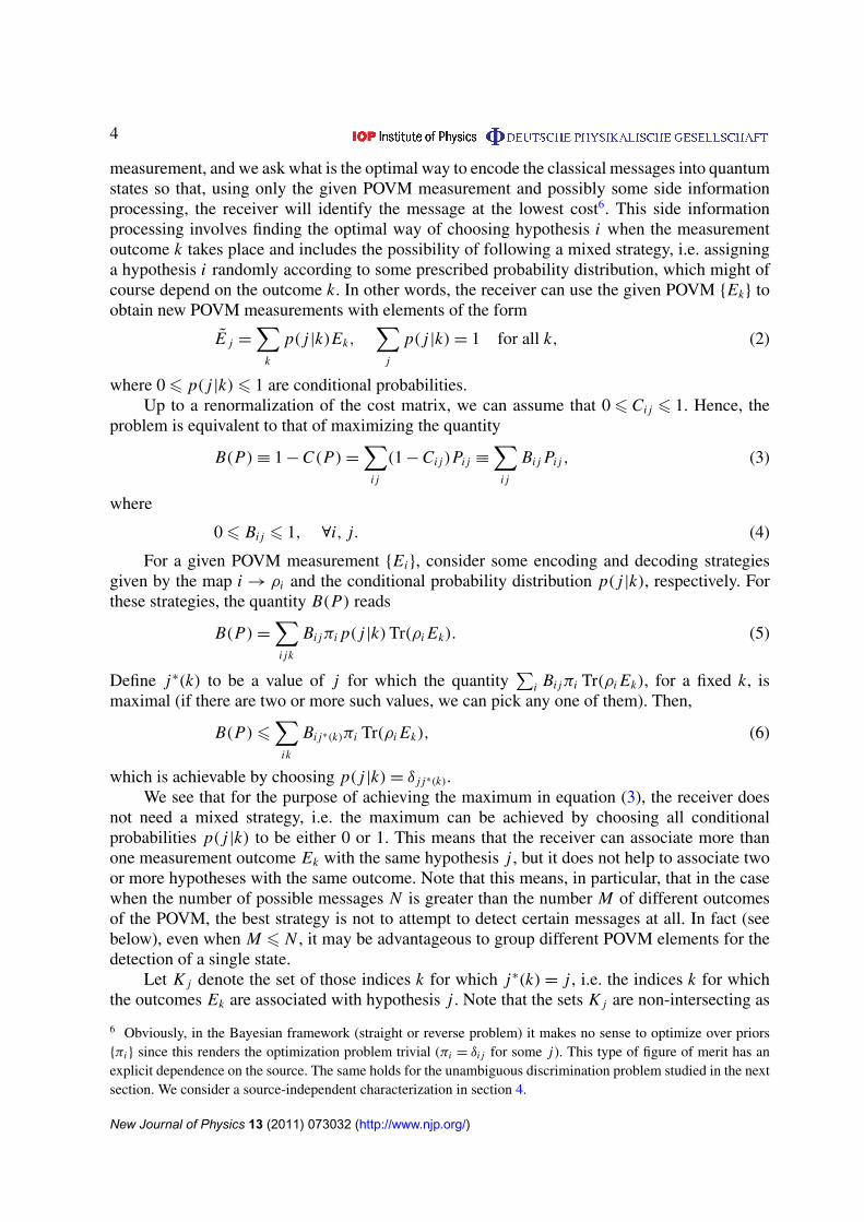
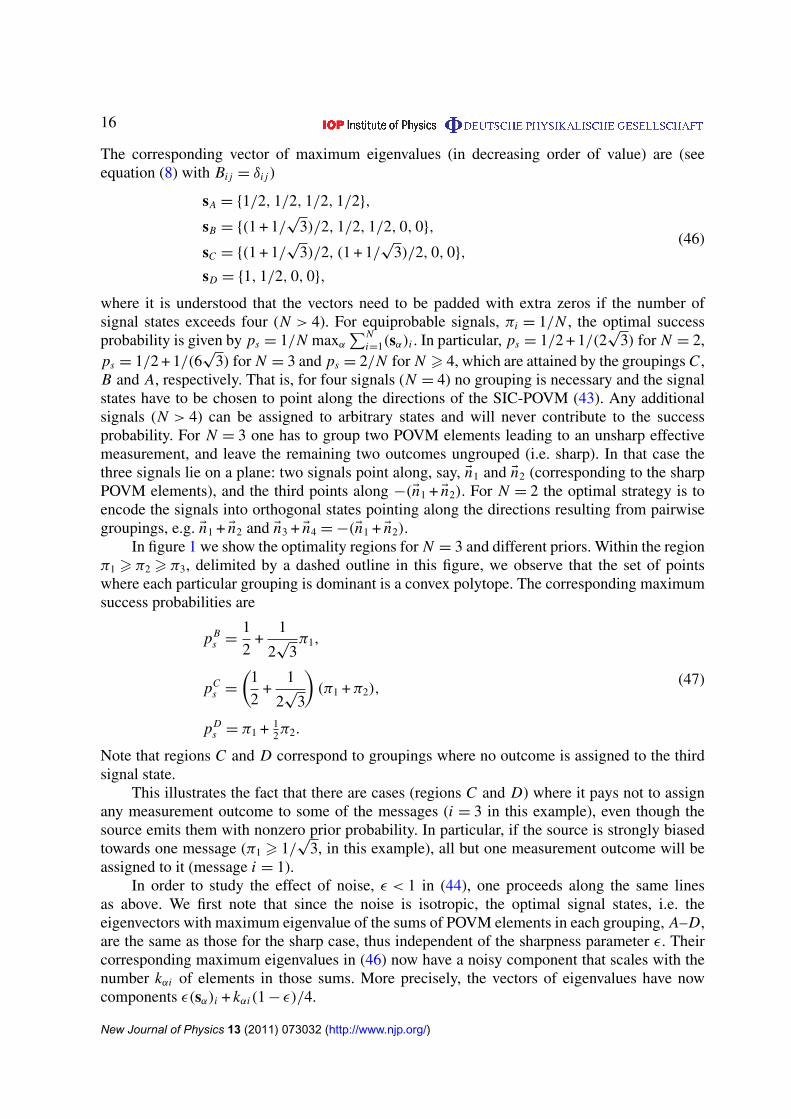
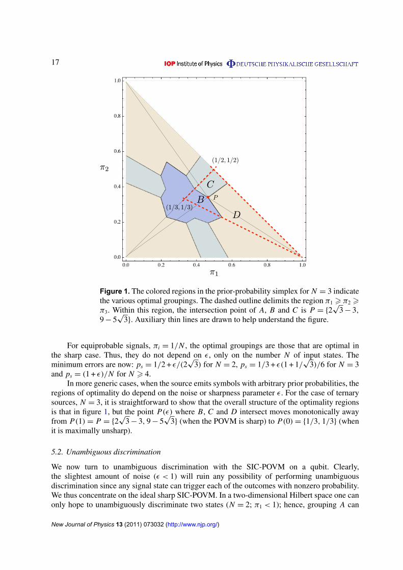
In figure 1 we show the optimality regions for N = 3 and different priors. Within the regionπ1 > π2 > π3, delimited by a dashed outline in this figure, we observe that the set of pointswhere each particular grouping is dominant is a convex polytope. The corresponding maximumsuccess probabilities are

pBs =

1

2+

1

2√

3π1,

pCs =

(1

2+

1

2√

3

)(π1 +π2),

pDs = π1 + 1

2π2.

(47)

Note that regions C and D correspond to groupings where no outcome is assigned to the thirdsignal state.

This illustrates the fact that there are cases (regions C and D) where it pays not to assignany measurement outcome to some of the messages (i = 3 in this example), even though thesource emits them with nonzero prior probability. In particular, if the source is strongly biasedtowards one message (π1 > 1/

√3, in this example), all but one measurement outcome will be

assigned to it (message i = 1).In order to study the effect of noise, ε < 1 in (44), one proceeds along the same lines

as above. We first note that since the noise is isotropic, the optimal signal states, i.e. theeigenvectors with maximum eigenvalue of the sums of POVM elements in each grouping, A–D,are the same as those for the sharp case, thus independent of the sharpness parameter ε. Theircorresponding maximum eigenvalues in (46) now have a noisy component that scales with thenumber kαi of elements in those sums. More precisely, the vectors of eigenvalues have nowcomponents ε(sα)i + kαi(1 − ε)/4.

New Journal of Physics 13 (2011) 073032 (http://www.njp.org/)

17

B

C

D

π1

π2(1/2, 1/2)

(1/3, 1/3)P

D/3

B3)

Figure 1. The colored regions in the prior-probability simplex for N = 3 indicatethe various optimal groupings. The dashed outline delimits the region π1 > π2 >π3. Within this region, the intersection point of A, B and C is P = {2

√3 − 3,

9 − 5√

3}. Auxiliary thin lines are drawn to help understand the figure.

For equiprobable signals, πi = 1/N , the optimal groupings are those that are optimal inthe sharp case. Thus, they do not depend on ε, only on the number N of input states. Theminimum errors are now: ps = 1/2 + ε/(2

√3) for N = 2, ps = 1/3 + ε(1 + 1/

√3)/6 for N = 3

and ps = (1 + ε)/N for N > 4.In more generic cases, when the source emits symbols with arbitrary prior probabilities, the

regions of optimality do depend on the noise or sharpness parameter ε. For the case of ternarysources, N = 3, it is straightforward to show that the overall structure of the optimality regionsis that in figure 1, but the point P(ε) where B, C and D intersect moves monotonically awayfrom P(1)= P = {2

√3 − 3, 9 − 5

√3} (when the POVM is sharp) to P(0)= {1/3, 1/3} (when

it is maximally unsharp).

5.2. Unambiguous discrimination

We now turn to unambiguous discrimination with the SIC-POVM on a qubit. Clearly,the slightest amount of noise (ε < 1) will ruin any possibility of performing unambiguousdiscrimination since any signal state can trigger each of the outcomes with nonzero probability.We thus concentrate on the ideal sharp SIC-POVM. In a two-dimensional Hilbert space one canonly hope to unambiguously discriminate two states (N = 2; π1 < 1); hence, grouping A can

New Journal of Physics 13 (2011) 073032 (http://www.njp.org/)

18

be excluded as it has too many outcomes. Moreover, we need only consider groupings B andD, since only they have at least one rank-one POVM element and have therefore a non emptykernel (K α

j 6= ∅). If grouping B is used, two messages can be unambiguously identified bychoosing the signals in the kernels of E3 and E4, respectively, that is, ρ1 = (1 − En3 · Eσ)/2 andρ2 = (1 − En4 · Eσ)/2, so that outcome 4 can only be triggered by ρ1 and outcome 3 by ρ2 (i.e.E1 = E4, E2 = E3 and E ? = E1 + E2). This leads to a probability of successful identificationgiven by

pBs = π1 Tr(E1ρ1)+π2 Tr(E2ρ2)

=1 − En4 · En3

4=

1

3, (48)

which is independent of the prior probabilities {π1, π2}.Proceeding along the same lines, one finds that for grouping D one can only

unambiguously identify the state ρ1 = (1 + En4 · Eσ)/2 with E1 = E4, by excluding ρ2 = (1 −

En4 · Eσ)/2 (i.e. ρ2 ∈ ker E1), while all other outcomes of the original POVM will be necessarilyinconclusive (E ? = I − E4). Obviously, no outcome will be associated with message i = 2(E2 = 0). The success probability is

pDs = π1 Tr(E1ρ1)=

π1

2, (49)

which beats that of grouping B for π1 > 2/3.

5.3. Mutual information

The SIC-POVM on a qubit, including its noisy version, is covariant under the tetrahedral group(indeed, the tips of the Bloch vectors (43) corresponding to the POVM elements define thevertices of a tetrahedron). Therefore, according to theorem 1 in section 4, the mutual informationfor this POVM is maximized by an ensemble of pure input states possessing the same symmetry.Its maximal value, i.e. the capacity of the measurement, is given by equation (32) for a state ψfrom the optimal ensemble (all other states in the ensemble are obtained from ψ by applyingoperators of the symmetry group, i.e. ψ plays the role of a ‘seed’ for the ensemble).

Theorem 2. (Capacity of the noisy two-level SIC-POVM). For every value of ε ∈ [0, 1], theseed ψ that maximizes expression (32) can be chosen such that its Bloch vector is anti-parallelto the Bloch vector of any one of the four POVM elements (44), i.e. Ev = −En j . The capacity ofthe (generally noisy) SIC-POVM is

Cε = 1 +1 − ε

4log

1 − ε

2+ 3

1 + ε/3

4log

1 + ε/3

2. (50)

This result, which applies to both the straight and the reverse formulations of the problem,is interesting in its own right. As far as we are aware, previous results (for ε = 1) relied onnumerical optimization [2]. Here we provide an analytical proof for 06 ε 6 1.

Proof. Let us define

h(t)≡ η

(1 + t

2

).

New Journal of Physics 13 (2011) 073032 (http://www.njp.org/)

19

We will first show that the following inequality holds for −16 t 6 1 and 06 ε 6 1:

h(εt)> a(ε)+ b(ε)t + c(ε)t2≡ ℘ε(t), (51)

wherea(ε)=

116 [h(−ε)+ 15h(ε/3)− 4εh′(ε/3)],

b(ε) =18 [−3 h(−ε)+ 3h(ε/3)+ 4εh′(ε/3)],

c(ε) =316 [3h(−ε)− 3h(ε/3)+ 4εh′(ε/3)],

and h′ is the derivative of h with respect to its argument.We start by noting the following relations,

℘ε(−1)= h(−ε), ℘ε(1/3)= h(ε/3), ℘ ′

ε(1/3)= εh′(ε/3) (52)

and

γ (ε)≡ c(ε)+ε2

4 ln 26 0, (53)

where the equality is attained only at ε = 0. The first three of them are immediate. The last oneis not so obvious and can be proved as follows. The function γ (ε) is concave in [0, 1] since

γ ′′(ε)= −9

2(1 − ε)(3 + ε)2 ln 2+

1

2 ln 2= −

ε(3 + 5ε + ε2)

2(1 − ε)(3 + ε)2 ln 26 0.

Differentiating the expression of c(ε) above, we readily obtain

c′(ε)=3

16 [−3h′(−ε)+ 3h′(ε/3)+ 43εh′′(ε/3)],

which vanishes at ε = 0. Thus γ ′(0)= γ ′′(0)= 0 and γ ′′(ε) < 0 if ε > 0. Then, γ (ε) mustnecessarily decrease for ε > 0, which in turn implies that γ (ε) has its unique maximum atε = 0. Since γ (0)= 0, equation (53) holds in the whole interval [0, 1].

We can now turn to proving (51). We assume that ε > 0, since ε = 0 is a trivial case. Iff (t)= h(εt)−℘ε(t), then

f ′′(t)= −2c(ε)−ε2

2(1 + ε t) ln 2.

It follows from this equation that there is only one value of t for which f ′′(t) vanishes. Butusing (53), we see that f ′′(t) > 0 for t > 0. Therefore, f ′′(t) can only change sign at somet0 < 0. Hence, f (t) is convex in (t0, 1] and concave in [ − 1, t0). It can have only one minimumin (t0, 1], and according to the third relation (52), it must be at t = 1/3. Using the secondrelation (52), we see that this minimum value is 0. Thus f (t)> 0 if t ∈ [t0, 1]. Because ofthe concavity of f in the other interval, we just need to check the value of f at the end pointt = −1 (by continuity we must have f (t0)> 0). The first relation (52) ensures that f (t)> 0also in [ − 1, t0].

Now, using the inequality (51), one can show that the mutual information for thePOVM (44),

I = 1 −1

2

4∑j=1

η

(〈φ|E j(ε)|ψ〉

tr E j(ε)

)= 1 −

1

2

4∑j=1

h(ε Ev · En j

),

New Journal of Physics 13 (2011) 073032 (http://www.njp.org/)

20

is bounded as

I 6 1 −1

2

4∑j=1

℘ε(Ev · En j)= 1 −1

2

[4a(ε)+

4

3c(ε)

]= 1 −

h(−ε)+ 3h(ε/3)

2.

This bound is attained with any one of the four choices Ev = −En j . The value of the capacity (50)is obtained by a straightforward substitution. ut

Note that in the minimum error scenario, the optimal signal ensemble is such that eachstate and its corresponding POVM element have maximum overlap (i.e. they are aligned witheach other). In contrast, here we find that it pays to have a signal ensemble where each statewould be excluded by one of the POVM outcomes in the absence of noise (i.e. states andPOVM elements are anti-aligned with each other). This configuration minimizes the (average)conditional entropy of the output (the POVM outcomes) given the input signal ensemble (recallthat the mutual information (32) can be obtained by subtracting this conditional entropy fromthe entropy of the output, which is constant here).

As expected, the capacity attains its maximal value C1 = log 4/3 for ε = 1 (the ideal SIC-POVM) and monotonically decreases towards 0 as ε approaches 0. Note that, as pointed out incorollary 2, the capacity of such a group covariant POVM is equal to the accessible informationof an equiprobable ensemble of states proportional to the original POVM elements,

ρi =I + εEni · Eσ

2, i = 1, 2, 3, 4. (54)

The latter problem, in the case ε = 1, was studied in [2], where it was shown that the accessibleinformation of the corresponding ensemble is A = log 4/3, which is equal to C1. The capacityof the ideal SIC-POVM has also been obtained by a different approach in [19].

6. Conclusion

In summary, we have studied the problem of optimal signal states for information readout witha given quantum detector. We considered some of the most common information transmissionproblems—the Bayes cost problem, unambiguous message discrimination and the maximalmutual information. We provided solutions to the Bayesian and unambiguous discriminationstrategies. We also showed that the maximal mutual information is equal to the classicalcapacity of the measurement and studied its properties in certain special cases. For a groupcovariant measurement, we obtained that the problem is equivalent to the problem of accessibleinformation of a group covariant ensemble of states. As an example, we applied our results onthe different discrimination strategies to the case of a SIC-POVM on a qubit, including a noisyversion of that POVM.

An interesting question for a future investigation is whether and under what conditions theoptimal solutions provided here are unique. Another question of significant interest would beto obtain an upper bound on the capacity of a measurement. We provided a lower bound whichis obtained from a lower bound on the accessible information, but that lower bound could alsobe improved. It would also be interesting to investigate the continuity properties of the optimalquantities considered in this paper. For example, if two measurements are close in terms of thedistance functions introduced in [32], are their capacities also close?

New Journal of Physics 13 (2011) 073032 (http://www.njp.org/)

21

Finally, we note that the capacity of a POVM provides a very natural and source-independent means of giving a quantitative characterization of a generalized quantummeasurement. However, it cannot be used as the unique figure of merit against whichmeasurement devices should be benchmarked. Ultimately, the performance of a givenmeasurement apparatus depends strongly on the task that it is meant to accomplish. Forinstance, a noisy Stern–Gerlach measurement might have a higher capacity than that ofan ideal SIC-POVM; however, it would be misleading to claim that such a Stern–Gerlachmeasurement outperforms the SIC-POVM since the latter can carry out tasks (e.g. full single-qubit tomography or unambiguous state discrimination) that are impossible to achieve with theformer.

Note added. Almost simultaneously with the posting of this paper, two concurrent worksappeared—by M Dall’Arno, G M D’Ariano and M F Sacchi (see [33]) and by A S Holevo(see [34])—which also introduce and study the capacity of a POVM measurement.

Acknowledgments

We thank Alex Monras for valuable discussions. This work was supported by the SpanishMICINN through the Ramón y Cajal program (to JC), contract number FIS2008-01236, andproject QOIT (CONSOLIDER2006-00019), and by the Generalitat de Catalunya through CIRIT2009SGR-0985. OO was partially supported by the Interuniversity Attraction Poles program ofthe Belgian Science Policy Office, under the grant IAP P6-10 ‘photonics@be’. EB thanks theHET group at BNL and Hunter College of the CUNY for their hospitality during the final stagesof this work. EB acknowledges financial support from the Spanish MICINN, reference numberPR2010-0367.

References

[1] Helstrom C W and Kennedy R S 1974 IEEE Trans. Inf. Theory 20 16[2] Davies E B 1978 IEEE Trans. Inf. Theory 24 596[3] Ivanovic I D 1987 Phys. Lett. A 123 257[4] Dieks D 1988 Phys. Lett. A 126 303[5] Peres A 1988 Phys. Lett. A 128 19[6] Fuchs C A 1996 Distinguishability and accessible information in quantum theory PhD Thesis University of

New Mexico, Albuquerque, NM[7] Chefles A and Barnett S M 1998 Phys. Lett. A 250 223[8] Raynal P and Lütkenhaus N 2005 Phys. Rev. A 72 022342[9] Lundeen J S et al 2009 Nat. Phys. 5 27

[10] Marcus M and Minc H 1992 A Survey of Matrix Theory and Matrix Inequalities (New York: Dover)[11] Elron N and Eldar Y C 2007 IEEE Trans. Inf. Theory 53 1900[12] Holevo A S 1998 IEEE Trans. Inf. Thy. 44 269–73[13] Schumacher B and Westmoreland M D 1997 Phys. Rev. A 56 131–8[14] Horodecki M, Shor P W and Ruskai M B 2003 Rev. Math. Phys. 15 629[15] Shor P W 2002 J. Math. Phys. 43 4334[16] Holevo A S 1998 Russ. Math. Surv. 53 1295 (arXiv:quant-ph/9809023)[17] King C 2002 J. Math. Phys. 43 1247[18] Hughston L P, Josza R and Wootters W K 1993 Phys. Lett. A 183 14

New Journal of Physics 13 (2011) 073032 (http://www.njp.org/)

22

[19] Hall M J W 1997 Phys. Rev. A 55 100[20] Jozsa R, Robb D and Wootters W K 1994 Phys. Rev. A 49 668[21] Kholevo A S 1979 Probl. Peredachi Inf. 15 3 (in Russian)[22] Zauner G 1999 Quantum designs—foundations of a non-commutative theory of designs PhD Thesis

University of Vienna (in German)[23] Renes J M, Blume-Kohout R, Scott A J and Caves C M 2004 J. Math. Phys. 45 2171[24] Prugoveki E 1977 Int. J. Theor. Phys. 16 321[25] Busch P 1991 Int. J. Theor. Phys. 30 1217[26] Caves C M, Fuchs C A and Schack R 2002 J. Math. Phys. 43 4537[27] Fuchs C A and Sasaki M 2003 Quantum Inf. Comput. 3 377[28] Fuchs C A 2002 arXiv:quant-ph/0205039[29] Oreshkov O and Brun T A 2005 Phys. Rev. Lett. 95 110409[30] Rapcan P, Calsamiglia J, Munoz-Tapia R, Bagan E and Buzek V 2011 arXiv:1105.5326[31] Reza F M 1961 An Introduction to Information Theory (New York: McGraw-Hill)[32] Oreshkov O and Calsamiglia J 2009 Phys. Rev. A 79 032336[33] Dall’Arno M, D’Ariano G M and Sacchi M F 2011 Phys. Rev. A 83 062304[34] Holevo A S 2011 arXiv:1103.2615.

New Journal of Physics 13 (2011) 073032 (http://www.njp.org/)