Electronic copy available at: http://ssrn.com/abstract=1990828

 

 

New Evidence on the Financialization of Commodity Markets*

Brian J. Henderson† The George Washington University

Neil D. Pearson††

University of Illinois at Urbana-Champaign

Li Wang‡ University of Illinois at Urbana-Champaign

May 24, 2012

Abstract

Following the recent, dramatic increase in commodity investments by financial institutions, academics, practitioners, and regulators have engaged in a heated debate over whether financial institutions’ trades and holdings have affected commodity prices and their return dynamics. Distinct from the prior literature, this paper examines the price impact of commodity investments on the commodities futures markets using a novel dataset of Commodity-Linked Notes (CLNs). CLN issuers hedge their liabilities by taking long positions in the underlying commodity futures on the pricing dates. These hedging trades are plausibly exogenous to the contemporaneous and subsequent price movements, allowing us to identify the price impact of the hedging trades. We find that these hedging trades cause significant price changes in the underlying futures markets, and therefore provide direct evidence of the impact of “financial” trades on commodity futures prices.

Keywords: Financialization, commodity-linked notes, commodity structured products, commodity index investors, commodity futures

                                                            * We thank seminar participants at the University of Illinois at Urbana-Champaign, University of

Massachusetts, and the FDIC’s 22nd Annual Derivatives and Risk Management Conference for comments and suggestions, and thank Ke Tang for a helpful discussion.

†E-mail: bjhndrsn@gwu.edu. The George Washington University, Department of Finance, Funger Hall Suite 502, 2201 G ST NW, Washington DC, 20052. Phone (202) 994-3669.

††E-mail: pearson2@illinois.edu. The University of Illinois at Urbana-Champaign, Department of Finance, 419 Wohlers Hall, 1206 South Sixth Street, Champaign IL 61820. Phone (217) 244-0490.

‡ E-mail: liwang2@illinois.edu. The University of Illinois at Urbana-Champaign, Department of Finance, 340 Wohlers Hall, 1206 South Sixth Street, Champaign IL 61820.

Electronic copy available at: http://ssrn.com/abstract=1990828

 

 

New Evidence on the Financialization of Commodity Markets

 

Abstract

Following the recent, dramatic increase in commodity investments by financial institutions, academics, practitioners, and regulators have engaged in a heated debate over whether financial institutions’ trades and holdings have affected commodity prices and their return dynamics. Distinct from the prior literature, this paper examines the price impact of commodity investments on the commodities futures markets using a novel dataset of Commodity-Linked Notes (CLNs). CLN issuers hedge their liabilities by taking long positions in the underlying commodity futures on the pricing dates. These hedging trades are plausibly exogenous to the contemporaneous and subsequent price movements, allowing us to identify the price impact of the hedging trades. We find that these hedging trades cause significant price changes in the underlying futures markets, and therefore provide direct evidence of the impact of “financial” trades on commodity futures prices.

Keywords: Financialization, commodity-linked notes, commodity structured products, commodity index investors, commodity futures

Electronic copy available at: http://ssrn.com/abstract=1990828

1

 

1. Introduction

Following several highly publicized reports espousing the historical diversification

benefits of exposure to commodity futures,1 in recent years financial institutions have increased

dramatically their investments in commodity futures. For example, according to an oft-cited

report, the value of index-related commodities futures investments grew from $15 billion during

2003 to over $200 billion during 2008.2 The period of most rapid growth in investments

coincided with the 20072008 boom in commodity prices, leading to heated debate among

academics, practitioners, and regulators regarding whether or not these “financial” flows

influence commodity futures prices and return dynamics. The question of whether financial

investors have affected prices through their increased participation in this market remains

unresolved.3 We contribute to this debate by analyzing a unique dataset of Commodity Linked

Note (CLN) issuances marketed to retail investors. Each of the sample CLNs is issued by and is

an obligation of a financial institution but has a payoff linked to the price of a single commodity,

commodity futures contract, commodities index, or basket of commodities futures. To hedge its

liability, the issuer trades in the commodities futures markets, typically establishing a long

position in near-term contracts. Importantly, CLN issuances are not based on information and

the hedging trades are plausibly exogenous to the contemporaneous and subsequent price

movements, providing clean identification of the price impacts of the hedging trades.

We find that CLN issuers’ hedging trades associated with products referencing individual

commodities have significant price impact on the referenced commodities’ futures prices,

providing evidence that investment flows that do not convey information nonetheless affect

prices. The issuers’ initial hedging trades for issues with proceeds greater than or equal to $2

million, $5 million, and $10 million raise the underlying commodity futures prices by an average

of 37, 40, and 51 basis points, respectively, around the pricing dates of the CLNs. We find

similar results for each of five different underlying commodity sectors, these being agricultural

commodities, energy commodities, industrial metals, platinum and palladium, and gold and

silver. We also find similar results around the pricing dates of products linked to commodity

baskets consisting of small numbers of commodities. However, we find no evidence of price

                                                            1 See for example Erb and Harvey (2006), Gorton and Rouwenhorst (2006), and Ibbotson and Associates (2006). 2 CFTC Staff Report (2008). 3 Irwin and Sanders (2011) refer to this question as a “Bubble” issue and provide a thorough literature survey. Irwin and Sanders (2011) use “commodity index fund” or “index fund” to refer to all commodity investment instruments.

2

 

impacts around the pricing dates of CLNs based on diversified commodity indexes. Additionally,

we find that very small CLN issues, defined as those with proceeds less than $2 million, do not

impact commodity futures prices.

With the development of commodity investment instruments and considerable investment

funds flowing into commodity index funds,4 some researchers have argued that the financial

sector gained influence relative to the real sector in determining the price level and return

dynamics of commodity prices, a phenomenon that is referred to as the “financialization” of

commodities. Theoretical arguments indicate that futures prices reflect both systematic risk

premiums (Black 1976, and Jagannathan 1985) and hedging pressures from the net hedging

demand of commodities producers and suppliers (Keynes 1930, Hicks 1939, Stoll 1979,

Hirshleifer 1988, and Bessembinder 1992). According to the financialization hypothesis, the

increased demand for long positions by financial investors, which are neither hedgers nor

traditional speculators in this market, is of large enough magnitude to affect the market prices

and return dynamics. Whether or not these flows from financial investors have impacted the

prices and return dynamics of commodities futures is the subject of considerable debate in the

recent literature.

One branch of the recent literature focuses on the relation between net positions of non-

commercial traders and futures price changes. This research employs the Commodity Index

Trader (CIT) supplement to the Commitments of Traders (COT) weekly report5 to construct

investment flows by index traders and studies their relation with futures prices. For the oil

market, Singleton (2011) finds a link between investor flows and futures prices, consistent with

the financialization hypothesis. A criticism of the CIT report data stems from the aggregation of

positions by category as opposed to separating the index traders’ positions for different trading

purposes.6 Another subset of this literature analyzes the return correlations between commodity

futures prices and other financial assets (e.g., stocks or bonds) or the co-movement among

commodities futures prices to determine the extent to which commodity markets have been

influenced by financialization. This part of the literature is motivated by the view of “financial”

                                                            4 Tang and Xiong (2010) and Irwin and Sanders (2011) provide detailed data summarizing the evolution of commodity index funds. 5 The CIT was initiated in 2007 and reports the aggregate positions of Commodity Index Traders in selected agricultural markets. 6 See, for example, Gilbert (2010), Tang and Xiong (2010), and Buyuksahin and Robe (2011). 

3

 

investors as index investors who focus on the strategic portfolio allocation between commodities

and other asset classes and thus tend to trade in and out of many commodities at the same time,

especially the commodities in one or more of the leading commodity indexes (Tang and Xiong

2010). This argument predicts that financialization causes price co-movements between

commodities futures and other major asset classes to increase, and that co-movement among

index commodities should rise relative to those not in the indices. Although researchers

generally agree that correlations increased during the recent financial crisis (Silvennoinen and

Thorp 2010 and Tang and Xiong 2010), some have pointed out that that even though the

correlations between equity and commodity returns increased dramatically in the fall of 2008, the

correlations remained lower than their peaks in the previous decade when commodity index

investment was not yet popular (Buyuksahin, Haigh and Robe 2010).

Many of the studies that fail to find evidence that financial investors’ positions impact

commodity futures prices rely on vector autoregressions and so-called Granger causality tests.

This approach involves regressing percentage or log changes in futures prices on lagged futures

price changes and lagged changes in some measure or measures of investors’ positions.

Researchers then interpret insignificant estimates of the coefficients on the variables measuring

lagged changes in financial investors’ positions as a lack of evidence that financial investors’

demands impact futures prices, while significant coefficient estimates would be interpreted as

evidence that changes in financial investors’ positions impact prices. A limitation of this

approach is that commodity futures prices rapidly incorporate information, including the

information in order flows, implying that the most likely causal channel comes through

contemporaneous changes in investors’ positions to changes in futures prices, not from lagged

changes in investors’ positions. The vector autoregressions using lagged position changes are

incapable of producing evidence that contemporaneous changes in investors’ positions impact

futures prices, because contemporaneous changes in investors’ positions are not included in the

regressions. Possible alternative regressions of changes in futures prices on contemporaneous

changes in investors’ positions are unidentified because over any interval contemporaneous

returns can cause changes in investors’ positions7 and also because both the commodity price

                                                            7 Specifically, any such analysis must use a time period of finite length. Changes in investors’ positions over some later part of the time period, say the second half of the period, can be caused by futures price changes over the first half of the period. This creates correlation between changes in futures prices and investors’ positions measured over the same time period.

4

 

changes and the changes in investor positions can be caused by an omitted common factor, e.g.

information that became available to some market participants.

Our approach overcomes the identification problem because the trades that hedge CLNs

sold to retail investors are plausibly exogenous. Specifically, the issuer ordinarily will execute

the hedge trades regardless of changes in futures prices, eliminating the “reverse causality” from

commodity futures price changes to trades and changes in positions. In addition, it seems

unlikely that retail investors base their purchases of CLNs on information about future changes

in futures prices because the issuers’ costs of structuring, marketing, and hedging the CLNs

render the CLNs high cost financial products.8 CLN issuers must embed these costs in the CLNs’

issue prices, negatively impacting CLN returns and making them poor vehicles for speculating

on changes in commodity futures prices. Further, the CLNs provide no or very limited leverage.

It seems unlikely that investors sophisticated enough to possess valuable information about

future commodity prices choose to trade on that information using high-cost, unlevered CLNs

rather than low-cost, liquid futures contracts that provide levered returns.9 CLN issues are

unlikely to be based on the issuers’ private information because the issuers typically hedge their

exposure to the underlying commodity prices and their main objective is to profit from the

embedded fees rather than to trade on information about the future commodity futures prices.10

The CLN issuances provide a convenient laboratory to study the impact of hedging trades

because the offering documents specify the CLNs’ pricing dates and indicate that the CLNs price

at the close of regular trading in the underlying commodity futures or commodity index. Since

the issuers hedge their liabilities associated with CLNs close to when the notes are priced, we are

able to determine the approximate dates and times when the issuers execute the hedge trades.

Thus, we are able to determine the approximate times when large “financial” trades in the futures

market are executed. Therefore, the pricing date price impact of the CLN issuances provides

direct evidence on whether such “financial” trades impact commodity futures prices.

                                                            8 Henderson and Pearson (2011), among other studies, document the large issue premiums in structured notes linked to individual stocks and issued by financial institutions to predominantly retail investors. 9 A field survey by staff at United Nations (2011) showed that the financial investors rely primarily upon official statistics about the commodity markets and pay more attention to the financial market than to the fundamentals of the commodities. 10 To the extent that the CLN issuer chooses not to hedge an issue, the issuer’s exposure to the commodity price will be negative, i.e. an issuer who does not hedge or hedges only partially will benefit from decreases in commodity price. Thus, the positive price impacts we find cannot be explained by a hypothesis that the CLN issues cause other market participants to infer that the issuer has private information about future commodity prices.

5

 

Our approach has several additional advantages. First, by using the CLN data we are able

to avoid relying upon the criticized CIT data. Second, we analyze the impact of new flows into

long-only commodity index investment on the commodity futures markets. This differs from

studies focusing on the roll activity of a commodity index, such as Mou (2010) and Stoll and

Whaley (2010), which analyze trades for existing long-only commodity index investment and for

which the trades in the front-month and front-next contract net to zero. Third, our analysis

includes all commodity sectors, rather than simply the agricultural sector or crude oil.11

As indicated above, we find average price impacts of 37, 40, and 51 basis points around

the pricing dates of the commodity structured product issues with proceeds greater than or equal

to $2 million, $5 million, and $10 million, respectively. We find similar results for each of five

different underlying commodity sectors, and also for issues of products linked to commodity

baskets consisting of small numbers of commodities. These main results exclude issues that are

priced and sold during the “roll” of the popular S&P GSCI commodity index that occurs from

the 5th to 9th business day of each month, the so-called “Goldman roll,” because Mou (2010)

presents evidence that the heavy selling of the front-month contract by investors who track the

index causes the price of the front-month contract to be temporarily depressed. We repeat the

main analysis including issues sold during the Goldman roll and obtain results similar to our

main results, indicating that our main results are robust to the inclusion or exclusion of issues

sold during the Goldman roll. We also find that our results are robust to the choice of

benchmark used to compute the abnormal returns on the commodity futures contracts.

Additional regression analyses show that the pricing date price impacts are increasing in

the size of the CLN issues, which is a proxy for the magnitude of the hedging trade. We also

present evidence that our results are not due to a selection bias in which issuers tend to complete

CLN issues on days of positive returns.

The next section of the paper reviews the related literature. Section 3 briefly describes

the sample of CLN issues and the retail market for CLNs, and also indicates the sources of the

other data used in the analysis. Section 4 contains the main results regarding the price impact of

the hedging trades, while Section 5 shows that the results are robust to the inclusion or exclusion

of issues during the Goldman roll and to the choice of benchmark used to compute the abnormal

returns on the commodity futures contracts. Section 6 briefly concludes.                                                             11 Buyuksahin and Robe (2009) and Singleton (2011) are examples of recent papers focusing on specific sectors of commodities futures markets.

6

 

2. Related Literature

With the development of commodity investment instruments and considerable investment

funds flowing into commodity index funds,12 some researchers argue that the financial sector

gained influence relative to the real sector in determining the price level and return dynamics of

the commodity market, a phenomenon that is referred to as the “financialization” of commodities.

One branch of this literature focuses on the relation between the changes in futures prices and the

net positions of non-commercial traders. Masters (2008) attributed the boom in commodity

prices from 20072008 to institutional investors’ embrace of commodities as an investable asset

class. Gilbert (2010) examined the price impact of index-based investment on commodity

futures over the period 20062008 by constructing a quantity index based on the positions of

index traders in 12 agricultural commodities from the Commodity Index Trader supplement to

the CFTC’s weekly Commitments of Traders (COT) report. He estimated that the maximum

impact of index funds in the crude oil, aluminum, and copper markets is a price increase of 15%.

These results are based on the assumption that the quantity index is an adequate proxy for total

index-related investment, not just positions in agricultural commodities.

Another strand of this literature analyzes the return correlations between commodity

futures contracts and other financial assets (e.g., stocks or bonds) or the co-movements among

commodity futures prices to determine the extent to which commodity markets have been

influenced by financialization. Silvennoinen and Thorp (2010) predict that the return correlation

between commodities and other financial assets will rise due to the increase in commodity index

investment. They test this hypothesis during the financial crisis and find increasing integration

between commodities and financial markets. Tang and Xiong (2010) argue that as most index

investors focus on the strategic portfolio allocation between commodities and other asset classes,

they tend to trade in and out of all commodities in a chosen index at the same time. This

argument predicts that the price co-movement among indexed commodities should rise relative

to those not in the indices when commodity index investment increases. Tang and Xiong (2010)

find that since the early 2000s futures prices of non-energy commodities in the US have become

increasingly correlated with oil futures prices and that this trend is significantly more

pronounced for commodities in the two popular S&P GSCI commodity index and Dow Jones-

                                                            12 Tang and Xiong (2010) and Irwin and Sanders (2011) provide detailed data and figures depicting the evolution of the commodity index fund. 

7

 

UBS Commodity Index (“DJ-UBS”) than for commodities not in the indices. They also find that

this increasing co-movement cannot be explained by the increasing demand from emerging

markets such as China or by an inflation factor, consistent with their argument that the prices of

commodities are now driven by the commodity index investors’ behavior, reflecting a process of

financialization of commodities. Cheng, Kirilenko, and Xiong (2012) find evidence of increased

systematic risk in commodities futures markets resulting from the financialization of

commodities markets.

In contrast to the above referenced studies, a number of researchers argue from both

theoretical and empirical perspectives that commodity prices and return dynamics are not

affected by financialization, i.e. they are still determined by “real” fundamental factors.13

Buyuksahin, Haigh and Robe (2010) document that even though the correlations between equity

and commodity returns increased dramatically in the fall of 2008, they remained lower than their

peaks in the previous decade when commodity index investment was not yet popular. In contrast

to Tang and Xiong (2010), they found little evidence of a secular increase in spillovers from

equity to commodity markets during some extreme events. Irwin and Sanders (2011) challenge

the results in Tang and Xiong (2010) due to their reliance on the CIT supplement to the COT

weekly report to construct investment flows by index traders because the report does not separate

the index traders’ positions for different trading purposes, but instead uses their aggregate

positions by classified category.14 In addition, Irwin and Sanders (2011) argue that the

differences-in-differences approach used in Tang and Xiong (2010) may not control for some

fundamental factors that are common to all commodities in a given sector. For example, they

argue that inventory levels and shipping costs contain important information about fundamentals.

Failing adequately to consider market fundamentals may also lead to incorrect inferences in tests

of co-movement (Ai, Chatrath, and Song (2006)).

Buyuksahin and Robe (2011) employ daily, non-public data on individual trader positions

in seventeen U.S. commodity futures markets. This dataset is contract-specific for most trader

categories (including, importantly, for hedge funds), permitting Buyuksahin and Robe (2011) to

                                                            13 For example, Krugman (2008), Pirrong (2008), Sanders and Irwin (2008), Smith (2009), Irwin, Sanders and Merrin, (2009), Buyuksahin and Harris (2009), Buyuksahin and Robe (2009), Till (2009), Korniotis (2009), Hong and Yogo (2010), Stoll and Whaley (2010), and Power and Turvey (2011). Irwin and Sanders (2011) and Singleton (2011) survey the relevant literature. 14 See Gilbert (2010), Tang and Xiong (2010), and Buyuksahin and Robe (2011). 

8

 

distinguish traders’ positions at different contract maturities. In contrast to Tang and Xiong

(2010), Buyuksahin and Robe (2011) find that only hedge fund activity rather than index fund

activity is a significant factor explaining the recent increase in correlations between stock and

commodity returns after controlling for the business cycle and other economic factors. However,

the hedge fund data are ambiguous regarding the trading purpose because some funds may trade

based on information about fundamentals and others may follow “technical” trading rules

(Gilbert, 2010). Also, this daily index investment data does not overcome the previously

limitations of the CIT data for the energy and metal markets.

A recent paper by Mou (2010) provides support for the financialization hypothesis by

focusing on the practice whereby commodity index investors “roll” their positions in the front-

month futures contract into longer-dated contracts. They document that the price impact of this

rolling activity is both statistically and economically significant. Due to limits to arbitrage, this

publicly-known trading is able to impact futures prices. Singleton (2011) presents new evidence

from the crude oil futures market that there is an economically and statistically significant effect

of investor flows on futures prices, after controlling for returns in U.S. and emerging economy

stock markets, a measure of the balance-sheet flexibility of large financial institutions, open

interest, the futures/spot basis, and lagged returns on oil futures. He finds that the intermediate-

term (three month) growth rates of index positions and managed-money spread positions had the

largest impacts on futures prices and argues that such impact may be due to different opinions

about public information and learning processes. These results are subject to the previously

mentioned limitations of the CIT data.

In less directly related work, Cheng, Kirilenko and Xiong (2012) present evidence that

trades by financially stressed commodity index traders and hedge funds had important impacts

on commodity futures prices during the financial crisis. Hong and Yogo (2010, 2012) present

evidence that growth in open interest in commodity futures market predicts changes in the prices

of commodity futures contracts, inflation, and nominal interest rates.

3. The U.S. Retail Market for Commodity-Linked Notes

CLNs are issued by and are obligations of financial institutions and have payoffs linked

to the price or change in price of a commodity or commodity futures contract, commodity index,

or basket of commodities or commodity futures. Most CLN issuers have “shelf registrations”

through which they issue CLNs periodically, with features of specific issues described in pricing

9

 

supplements. Each pricing supplement includes the terms of the CLN, such as the maturity date,

participation (or leverage) rate, cap value (or maximum return), coupon rate, buffer level,

investor fee and other provisions that determine the final payoff to the investor. Importantly for

our analysis, the pricing supplements also include the pricing date (and time, e.g. the close of

trading) when issuers price the notes. The issues in our sample were priced as of the close of

trading in the underlying commodity on the pricing date. In anticipation of, or shortly after, the

sale of the CLNs, the issuers enter into hedging transactions. The typical CLN hedging trade

involves the purchase of related futures or swap contracts, or other instruments the value of

which derives from the underlying asset. When the issuer’s hedge transaction involves a

commodity swap or swaps, the swap counterparties typically rehedge in the futures markets. The

issuers file the pricing supplements describing the CLNs with the U.S. Securities and Exchange

Commission (SEC), which makes them available through its EDGAR database.

The sample consists of nearly the entire universe of publicly issued CLNs in the United

States with payoffs depending on the price or change in price of an individual commodity, a

basket of commodities, or a commodity index. We construct the sample by first identifying all

issuers of publicly registered CLNs in the United States.15 The sample consists of the publicly

registered CLNs issued by the 20 banks and other financial intermediaries identified as issuers.16

After identifying the issuers, we collect the 424(b) fillings for each issuer from the SEC’s

EDGAR website. We then process those filings to identify all CLN issues and extract the details

required for the analysis including the pricing date, product name, proceeds amount, reference

commodity, commodities, or commodity index, maturity date, and coupon rate.

The first sample CLN issue dates to January 17, 2003, when Swedish Export Credit

Corporation offered “90% Principal Protected Zero-Coupon GSCI Excess Return Indexed Notes.”

These notes promised to return to investors 90% of the principal amount plus a possible

additional return linked to the performance of the Goldman Sachs Commodity Index,17 and did

not pay any other interest. The first sample CLN referencing a single commodity consists of the

                                                            15 We identify issuers by searching Mergent’s FISD database for issues matching both keywords “commodity” and “link.” Additionally, we search www.quantumonline.com and the AMEX website for listed CLNs, and identity the issuers of the CLNs that we find. 16 The sample consists of CLNs issued by the following 20 issuers: ABN AMRO, AIG, Bank of America, Barclays, Bear Stearns, Citigroup, Credit Suisse, Deutsche Bank, Eksportfinans, Goldman Sachs, HSBC, JP Morgan, Lehman Brothers, Merrill Lynch, Morgan Stanley, RBC, Swedish Export Credit, UBS, Wachovia, and Wells Fargo. 17 This is the former name of the index now known as the S&P GSCI.

10

 

“Principal Protected Notes linked to Gold Bullion” issued by UBS during May 2003. These

notes guaranteed full principal payment at maturity plus a possible additional return capped at

21.4%.

As of August 2011, the total proceeds of publicly registered CLN issues exceed $60

billion, which amount is comparable to the market value of equity-linked notes based on

individual equities issued from 1994 to 2009 as reported in Henderson and Pearson (2010). By

August of 2011, the total outstanding amount of notes not yet called or matured is about $42

billion, which amounts to approximately 11% of the total commodity index investment.18 The

sample CLNs have payoff profiles linked to a large number of different assets, including those

comprising the most popular commodity indices, e.g., the S&P GSCI and the DJ-UBS, and also

commodities that are not in the leading indices, e.g. platinum and palladium.

Owning a CLN is not equivalent to owning the underlying commodity or commodity

futures contract. Importantly, payments to CLN holders are obligations of the issuing financial

institution and these payments are backed only by the creditworthiness of the issuing financial

institution. At maturity, the investor receives a cash payment as defined in the pricing

supplement rather than the underlying physical commodity or commodity futures contract.

The specific terms and features of the CLNs vary across products. The Accelerated

Return Notes (ARNs) linked to the Silver Spot Price priced and sold by Bank of America on

February 25, 2010 are an example of a popular product type. These ARNs had a face value and

issue price of $10 per unit, had a zero coupon rate, and matured on May 3, 2011. The starting

value of the reference commodity, the silver spot price as determined by London Silver Market

Fixing Ltd., was $15.92 on the pricing date. The notes’ payoff at maturity is based on the ending

value, which is the silver spot price as of the calculation date, April 26, 2011. If the change in

the spot price from the pricing date to the calculation date is positive the investors receive the

face value plus an additional payment equal to the product of the face value and three times the

percentage increase, capped at 34.26%. If the percentage change in the spot price is negative

then the principal amount returns to investors is reduced by the product of the percentage change

and the face value.

                                                            18 A report by the Institute of International Finance (2011) shows the total investment in commodity index-linked funds to be approximately $400 billion. Stoll and Whaley (2010) estimated that the total commodity index investment in the U.S. market in 2009 is about $174 billion. Of the total commodity index investors, 42% are institutional traders, 24% are index funds, and 25% are retail investors holding exchange-traded commodity products.

11

 

Some other CLNs include either an early redemption or an “auto-callable” feature. An

example comes from the iPath Dow Jones–AIG Agriculture Total Return Sub-Index ETN issued

by Barclays on October 23, 2007. These notes mature on October 22, 2037, do not pay interest,

and allow the holders to redeem their notes on any redemption date, defined as the third business

day following each valuation date. The valuation date is any business day between October 24,

2007 and October 15, 2037, inclusive. Upon redemption, investors receive cash payment in an

amount equal to (1) the principal amount times (2) the index factor on the applicable (or final)

valuation date minus (3) the investor fee on the applicable (or final) valuation date. The

investors must redeem at least 50,000 Securities at one time in order to exercise the redemption

right prior to final maturity. The index factor on any given day is equal to the closing value of

the Index on that day divided by the initial index level, which is the closing index level on the

pricing date. Investors pay a fee of 0.75% per year times the product of the principal amount and

the index factor.

Another popular CLN structure references a commodity index and pays monthly coupons

to investors. The notes linked to the Dow Jones-AIG Commodity Index Total Return issued by

the Swedish Export Credit Corporation in April 2006 are an example of such a structure. These

notes matured on March 30, 2007, and were redeemable by the issuer prior to maturity. On the

maturity or early redemption date, the notes promised investors an amount equal to the principal

amount times the leveraged index performance, defined as one plus the product of the leverage

factor, here 3, and the adjusted index performance factor. At maturity or upon redemption, the

investors also receive the supplemental amount that has accrued on the outstanding principal

amount of each note for the period from and including the issue date of the notes to the

applicable settlement date. The supplemental amount accrues at a rate equal to three-month U.S.

dollar LIBOR minus a spread of 0.24% per annum, as reset on the 30th day of June, September

and December, beginning June 30, 2006, compounded quarterly on each reset date.

Table 1 summarizes the numbers of CLN issues and the aggregate proceeds for various

groups of underlying commodities, by year. The sample used for this table includes almost all of

the publicly registered CLNs issued by the 20 main banks and financial intermediaries listed in

Table 2.19 For each sample year, beginning with 2003 and ending in August 2011, the table

                                                            19 The sample excludes several CLN issues by Swedish Credit Corporation because those issues were remarketing efforts of previously issued notes and the documents do not indicate the dates on which the additional notes were marketed and sold.

12

 

columns present the number of CLN issues and total proceeds (in thousands of dollars). The

CLNs are subdivided by the type of underlying reference commodity. Individual commodities

are grouped into the commodity sectors: Agriculture (corn, cotton, wheat, soybeans, coffee,

sugar, live cattle, lean hogs, soybean oil, soybean meals, red wheat, and cocoa), Energy (WTI

crude, Brent crude, natural gas, heating oil, and unleaded gasoline), Industrial Metals (Aluminum,

copper, lead, nickel, and zinc), Platinum and Palladium, and Gold and Silver. The table also

includes a category “Diversified Index and Commodity Baskets” CLNs based on diversified

indexes include products based on the DJ-UBS, S&P GSCI, Deutsche Bank Liquid Commodity

Index, and some other commodity indices, excluding products based on sub-indices. The

commodity baskets of more than one individual commodity are specified by the issuers. CLNs

based on a sub-index restricted to a single commodity sector are included with the CLNs based

on individual commodities in that sector.20

The rightmost column of Table 1 presents the annual CLN proceeds across all issuers.

Issuance across the full sample spanning 2003 through August 2011 totals nearly $59 billion.

The total proceeds of CLN issues during the 20072008 boom exceed $30 billion and account

for approximately 50% of the total amount issued during the full sample period. Similar to the

estimates of index investors’ position sizes by Stoll and Whaley (2009), CLN issuance proceeds

decline dramatically in 2009 to $13.2 billion. The number of CLN issues, however, remains

large at about 300 issues per year from 2008 through 2011. In the full sample of CLNs with

proceeds of over $59 billion, approximately 12% of the proceeds come from notes linked to

agricultural commodities, 36% from notes linked to energy commodities, 8% from notes linked

to industrial metals, 1% from notes linked to platinum and palladium, 10% from notes based on

gold and silver, and 33% from notes linked to a diversified commodities index or a basket of

more than one individual commodity. The bottom row of Table 1 reports the average proceeds

per issue for each of the reference categories. CLNs referencing energy commodities tend to be

the largest with average proceeds over $102 million. CLNs referencing Platinum and Palladium,

commodities which are not included in the major indexes, tend to be the smallest with average

proceeds of just over $20 million across the 33 sample observations.

                                                            20 For example, a CLN based on the S&P GSCI-Energy sub-index would be included with the CLNs based on individual energy commodities.

13

 

Table 2 presents the number of CLN issues and total proceeds for each issuer in the

sample. Similar to Table 1, the columns of Table 2 present the number of issues and total

proceeds (in thousands of U.S. dollars) for each issuer of CLNs. The first columns of the table

disaggregate the products linked to individual commodities by sector, followed by the issues

linked to an index or basket of more than one commodity, and finally the total number of CLNs

and proceeds for the issuers. Referring to the rightmost column, which aggregates the data

across all types of commodities at the issuer level, Barclays, Deutsche Bank, and Swedish Export

Credit issued the largest numbers of CLNs with 261, 186, and 171 issues, respectively. Based on

proceeds, Deutsche Bank and Barclays are the largest issuers, having raised over $23 billion and

$16 billion of proceeds, respectively. Among the other frequent issuers of CLNs, Bank of

America’s 119 offerings total over $2.7 billion proceeds, Merrill Lynch’s 51 offerings total more

than $2.6 billion, and Eksportfinans’s 64 issues total more than $2.5 billion. Scanning the

columns, one can see that some issuers such as Barclays are particularly active in issues linked to

particular underlying assets. For example, Barclays issued 51 out of a the total 132 CLNs linked

to agricultural commodities and10 out of 33 linked to platinum and palladium, but only 99 out of

842 linked to diversified indexes and baskets. Overall, the table makes clear that the sample of

1,491 CLN issues spans many issuers and reference assets.

4. Price Impact of the Hedging Trades

To measure the impact of CLN issuers’ hedging trades on commodity futures prices, we

focus on the returns of front-month futures contracts around the pricing dates, when issuers

execute trades to hedge the commodity exposures stemming from the CLNs. Unless the market

supply of futures contracts is perfectly elastic, large buy (sell) trades will raise (lower) futures

prices. This price impact should be increasing in the size of the issue (e.g., the price impact must

be zero if the trade size is zero), and there is a theoretical argument that the price impact of a

trade should be linear in the size of the trade (Huberman and Stanzl (2000)). For these reasons,

we expect to see significant price impacts around the pricing dates of CLN issues with large

proceeds. Also, because the hedging trades associated with an index linked product are spread

across many different contracts, price impacts around the pricing dates of the index products are

likely smaller and possibly undetectable.

As briefly indicated above, we examine CLN issuances because the hedging trades

associated with the issues constitute new buying pressure from financial investors that is not

14

 

based on contemporaneous returns or private information possessed by any market participant.

The issuer ordinarily will execute the hedge trades regardless of changes in futures prices during

the period when the hedge trades are being made, eliminating the possible “reverse causality”

from price changes to trades and changes in positions.

In addition, it seems unlikely that the CLN issuances convey to the market valuable

private information held by retail investors. The issuers’ costs of structuring, marketing, and

hedging the CLNs render them high cost financial products.21 CLN issuers must embed these

costs in the issue prices, negatively impacting CLN returns and making them poor vehicles for

speculating on changes in commodity futures prices. Further, the CLNs provide no or very

limited leverage. Finally, most CLNs suffer from illiquid secondary markets, rendering it costly

for a CLN investor to exit a position. The majority of the products are not exchange traded and

trade “over-the-counter” only infrequently, with the issuer typically being the only market

participant willing to provide a secondary market bid price.22

In contrast, underlying each CLN are one or more low cost, liquid, exchange-traded

futures contracts offering embedded leverage. Due to the ease of access, low cost, liquidity, and

embedded leverage of futures contracts, it seems likely that an investor who did possess valuable

private information about future commodity prices would prefer to trade on that information

using futures contracts rather than CLN’s.23 In order for one to believe that retail investors

buying CLNs possess valuable private information about future commodity prices, one must

believe that investors purchasing CLNs are sophisticated enough to possess valuable private

information, but so unsophisticated that that they are unaware that the futures contracts provide

a better vehicle for speculation.

Finally, it seems very unlikely that the CLN issuances convey issuers’ positive private

information to other market participants, because the issuers typically hedge their exposure to the

underlying commodity futures prices and thus have no or limited net exposure to the underlying

                                                            21 Examination of the pricing supplements reveals that the underwriter compensation is approximately 2% per issue, which is a lower bound on the initial over-pricing of these products. Other embedded costs include legal fees, hedging costs, and any other costs associated with designing and distributing the notes. Henderson and Pearson (2011), among other studies, document the large issue premiums in structured notes linked to individual stocks and issued by financial institutions to predominantly retail investors. 22 Some of the CLNs are listed and trade as exchange-traded notes. 23 In a different context, Black (1975) argues that the embedded synthetic leverage is an important reason why investors with valuable private information might prefer to take advantage of that information using options rather than the options’ underlying stocks. The same reasoning implies that an investor with information would prefer to trade futures contracts rather than purchase CLNs.

15

 

futures prices. To the extent that a CLN issuer chooses not to hedge a CLN issue or to hedge

only partially, the issuer’s exposure to the commodity price will be negative, i.e. an issuer who

does not hedge or hedges only partially will benefit from decreases in the underlying futures

price. Thus, the positive price impacts we document below cannot be explained by the

hypothesis that the CLN issues cause other market participants to infer that the issuer has private

information about future commodity prices.

4.1 Research design

To measure the price impact of CLN issuers’ hedging trades, the analysis uses the returns

on the front-month futures contract on the reference commodity, computed from futures price

data obtained from Bloomberg.24 The daily futures return is defined, as in Tang and Xiong

(2010), as

)ln()ln( ,1,,,, TtiTtiti FFR , (1)

where TtiF ,, is the date-t price of the front-month futures contract of commodity i with maturity

or delivery date T.  

The financial institutions issuing CLNs price and issue the notes based on the closing

market price of the reference commodity or commodity futures contract on the pricing date. We

collect the pricing date for each sample issue of publicly registered CLNs from the pricing

supplements available through the S.E.C.’s EDGAR database. Although the documents specify

the date and time when the issues are priced, the exact timing of the issuers’ hedge trades is not

clear. For example, the issuer may execute the entire hedge trade on the pricing date, or it may

delay a portion of the hedge trade until the next day in an effort to spread the price impact and

minimize the average purchase price of the futures contracts. For this reason, the analysis

focuses on the price impact over a two-day window encompassing the pricing date and the

following trading date.

For some CLNs, the issuers may hedge their obligations using commodity swaps traded

“over-the-counter.” In this case, the commodity swaps dealers in turn face the need to hedge

their swap positions, and typically do this by transacting in the futures market. Thus, the

hedging demand is passed through to the commodity futures markets, even when the initial                                                             24 Gorton and Rouwenhorst (2006), Tang and Xiong (2010), and Stoll and Whaley (2010) argue that the closest to expiring futures contract may be illiquid close to its expiration and the traders may use the next-closest-month expiring contract, the “front-next” contract. We repeated the main analyses using the front-next contract and obtained similar results.

16

 

hedge trades involve swaps.25 That said, over-the-counter swap dealers may have the ability to

net some exposures internally and thus might not pass all exposures through to the futures

market. To the extent that this happens, the hedge trades associated with CLNs might not

impact the futures market as much as hedge trades directly executed in the futures market by the

issuers, reducing the magnitude of our estimated impact. It has been estimated that swap dealer

netting is relatively small in agricultural futures markets, but that it can be large in the energy

and metals markets (CFTC 2008). Taking account of this, other things equal we expect a greater

price impact in the agricultural sector than in the energy sector or metal sector. Also, if the CLN

issuer hedges using swaps, it is possible that the swap counterparty will not immediately rehedge

in the futures market. This is another reason why we focus on the two-day futures market return.

The price impact should be increasing in the size of the hedge trade. For this reason, we

do not include small CLN issues in the analysis but instead focus on subsamples of products with

more sizeable proceeds so that we reasonably expect the issuers’ hedge trades to be large enough

to produce measurable price impact. Table 3, Panel A presents the number of issues and average

proceeds (in thousands of dollars) for the principal subsamples we use. The table describes three

subsamples: CLN issues with proceeds of at least $2, $5, and $10 million dollars. Referring to

Panel A, of the 1,491 issues in the full sample, 1,046 CLN issues have proceeds of at least $2

million, including 538 issues linked to individual commodities or baskets. The average proceeds

are sizeable, ranging from $24.7 million for issues linked to platinum and palladium to $152.5

million for issues linked to energy commodities. The subsample of CLNs with proceeds of at

least $10 million of proceeds consists of 590 issues, including 294 issues linked to individual

commodities or baskets and 296 issues linked to commodity indexes. The average issue sizes are

large for this subset, ranging from $44 million to $305 million depending on the underlying

commodity type.

The S&P GSCI “rolls” from the front-month futures contracts to the longer dated

contracts during a rolling period which spans the 5th to 9th business day of each contract maturity

                                                            25 This argument is illustrated by the following statement that appeared in a feature article in the May 2006 issue of Futures Industry magazine:

Keith Styrcula, chairman of the Structured Products Association, explains that one way a CLNs issuer can hedge its commodity exposure is through a total return swap with either its own swaps desk or a third party. The counterparty will then lay off the risk in the futures market. “At the end of the day, much of the hedging winds up creating open interest and volume in the underlying futures contracts. All roads lead to enhanced liquidity on the futures exchanges.” (O’Hara, 2006) 

17

 

month. During this period, 20% of the index rolls each day from the front-month futures

contracts to longer dated contracts. Mou (2010) finds that the roll produces downward price

pressure on the front-month futures contracts over this period for the commodities included in

the index and corresponding upward price pressure for the next-month contracts, i.e. that it

affects the futures price term structure. The hedging trades studied in this paper are different

from the rolling activity considered in Mou (2010) since they represent net inflows to the futures

market and impact the level of futures prices, as opposed to rebalancing along and impacting the

term structure. To keep our results separate and distinct from the roll effect, in the main analysis

we further restrict the sample to include only the issues having pricing dates that do not fall

during the S&P GSCI roll periods. Panel B of Table 3 presents the sample of large issues with

pricing dates that do not fall during index roll windows. The sample contains 837 CLN issues

with proceeds of at least $2 million and 476 with proceeds of at least $10 million. The average

proceeds are of similar magnitudes to those in Panel A.

We measure the price impact of the hedging trades using the daily abnormal return for

the reference commodity’s front-month futures contract. For each sample CLN issuance, i, with

pricing date t, we define the abnormal return ( , ) to the front-month futures contract on the

CLN reference commodity as

, , , , (2)

where , is the day t return to the front-month commodity contract for the underlying

commodity, defined as the difference in log daily closing futures prices: , log ,

log , . The benchmarked return ( , ) is estimated using a factor model capturing economic

effects likely to influence commodity futures returns.

The return benchmark includes variables likely related to contemporaneous changes in

commodities futures prices. As discussed by Tang and Xiong (2010) and Singleton (2011),

demand stemming from the growth in emerging market Asian economies has been an important

factor in commodity prices over the sample period. We include the returns to the MSCI

Emerging Markets Asia Index, , , to capture the impact of growth in emerging market Asian

economies on commodities prices. Because the futures contracts trade in the U.S. and the U.K.,

we account for non-synchronicity in close-to-close returns from different time zones by

including the next day return to this index, , . Inclusion of the S&P 500 index return,

& , , captures changes in demand due to U.S. economic growth. We include the returns to the

18

 

U.S. Dollar Index futures contracts, , , consistent with Tang and Xiong (2010) who control

for the strength of the U.S. Dollar as the dollar’s strength influences demand for commodities

and the dollar is the most common settlement currency for commodity transactions. Next, we

include the return to the JP Morgan Treasury Bond Index, , , to capture the link between

commodity demand and fluctuations in interest rates, as in Tang and Xiong (2010). To control

for the contemporaneous relation between commodities prices and innovations to the VIX index

found in Cheng, Kirilenko, and Xiong (2012), we include the contemporaneous percentage

change in the VIX index, , . We also include two additional control variables. The first is

the Baltic Dry Index, , which measures changes to the cost of transporting raw materials by

sea and proxies for commodity demand. The second macroeconomic control is the 10-year

breakeven inflation rate change, , as computed by Gürkaynak, Sack, and Wright (2010).

Calculation of the breakeven inflation rate involves comparison of the nominal yield curve and

the U.S. TIPS yield curve. Finally, we include the lagged commodity futures return to account

for autocorrelation, or persistence, in the return series. With the exception of the change in the

breakeven inflation rate, the data are obtained from Datastream and Bloomberg. The breakeven

inflation rate data are from the Board of Governors of the Federal Reserve System.26

Computation of the benchmark returns begins with estimation of the following regression

model for each observation:

, , , , , , & & , , , , , (3)

, , ,

, , .

For each sample observation, we estimate the benchmark model using data from the sixty trade

days immediately preceding the pricing date. For each sample observation, the expected return,

, , comes from the sum product of the estimated coefficients from Model (3) and the values of

the right hand side variables on the issuance date (X), i.e.

, . (4)

The commodity futures event-time abnormal return in equation (2) above is obtained by

subtracting the benchmark return computed using equations (3) and (4) from the log return in

equation (1). The next section presents the main results of the paper, which are the average

                                                            26 Breakeven inflation data are available at: http://www.federalreserve.gov/econresdata/researchdata.htm

19

 

abnormal commodity futures returns, or price impacts, surrounding issuance of CLNs linked to

individual commodities.

4.2. Individual commodities and commodity baskets

According to the financialization hypothesis, large inflows to commodity futures markets

from financial investors for the purpose of gaining passive, strategic allocation to commodities

affect prices in this market. The results in this section shed light on this topic by examining the

returns to commodity futures around CLN issuances. The finding that hedging trades in

commodities futures associated with the issuance of CLNs linked to individual commodities

impact the prices of those contracts constitutes compelling evidence that these exogenous, non-

fundamental trades impact prices by statistically and economically meaningful magnitudes.

The exact timing of the issuer’s hedging trades is not certain, and hedging policy may

vary across issuers. For example, an issuer may execute the entire hedging trade near the close

of trading on the pricing date, to coincide with the determination of the offering price.

Alternatively, the issuer may delay a portion of the hedging trade until the next day to minimize

market impact. Should an issuer hedge their exposure with an instrument other than futures

contracts, such as a commodity swap, although the swap dealer likely offsets its risk by buying

futures, the exact timing when the order flow reaches the futures market is uncertain. For these

reasons, the main analysis focuses on the price impact over the two-day event window spanning

the pricing date and the next subsequent trading day. We denote this two-day window as Days

[0,1]. Additionally, we present the abnormal returns on the pricing date, referred to as Day 0,

and the next day, Day +1.

For the sample of CLNs referencing individual commodities or baskets of commodities,

Table 4 presents the average abnormal returns for the front month underlying commodity futures

contracts. The averages presented in Table 4 include three subsets of products based on the issue

proceeds: issues totaling at least $2 million proceeds, at least $5 million proceeds, and at least

$10 million proceeds. The price impact, as measured by the abnormal return to the front month

futures contracts, should increase in the size of the hedge trade. The sample excludes issues

during the S&P GSCI roll window.

The first row of Panel A presents the average abnormal returns to the front-month futures

contracts. Across the three subsamples of large CLN issuances, the average abnormal returns on

the pricing date, Day 0, are positive and significant. For the sample CLNs having proceeds

20

 

greater than $2, $5, and $10 million, respectively, the Day 0 average abnormal returns are 21, 22,

and 30 basis points. The corresponding t-statistics (2.69, 2.39, and 2.93, respectively) indicate

statistical significance of the price impacts at conventional levels. The abnormal returns on the

trading day immediately following the pricing date, Day +1, are generally positive. This

evidence is consistent with issuers delaying a portion of the hedge trade. Abnormal returns over

the two day window, [0,1], are positive at 35, 37, and 48 basis points across the three subsamples.

Additionally, the t-statistics range from 2.88 to 3.25, indicating significance at conventional

levels. Consistent with the hypothesis that the abnormal returns stem from the issuers’ hedging

trades, the abnormal returns increase monotonically across the subsamples with increasingly

larger proceeds sizes. For all products having proceeds greater than $10 million, the Days [0,1]

abnormal returns average 48 basis points compared to 21 basis points for all CLN issuances

having at least $2 million proceeds. Under the assumption CLNs having greater proceeds

require larger hedge trades, the patterns in Table 4 are consistent with the interpretation that the

abnormal returns result from the price impact of order flow resulting from CLN issuers’ hedging

trades.

The next two rows of Table 4 present the number of positive and negative abnormal

returns in each subsample. The last row provides the probability that, under the null hypothesis

that the probability of a positive return is 0.5, the number of positive abnormal returns equals or

exceeds the number reported in the table. Specifically, the probability reported for date t is

Prob knkn

xk

n

kt ppxk

)1( , (5)

where tx is the number of positive returns observed on date t in the sample, knk ppk

n

)1( is

the probability of k positive abnormal returns out of a total of n observations, and 5.0p is the

probability of a positive abnormal return under the null hypothesis that positive and negative

returns are equally likely. All p-values for the two-day abnormal returns, [0,1], are less than 1%,

indicating that the numbers of positive two-day returns are significantly larger than the number

of non-positive returns for each sub-sample. For example, the sample of issues with proceeds of

at least $10 million contains 151 issues with positive two-day returns around the pricing date and

101 with negative returns. Under the null hypothesis, the probability that 151 out of 252 returns

are positive is less than 1%.

21

 

Panel B of Table 4 repeats the analysis from Panel A, but excludes CLN issues

referencing baskets of commodities. The results are similar to those presented in Panel A,

indicating that the results presented in Panel A are not driven by the inclusion of CLNs linked to

more than one commodity. The price impacts over the two-day period including CLN pricing

dates are positive and statistically significant. The magnitudes of the price impacts are nearly

identical to those in Panel A.

The results presented in Table 4 are consistent with the “financialization” of commodity

markets since commodities futures prices tend to increase on days when CLN issuers likely

execute hedging trades. These hedging trades appear to have statistically and economically

meaningful impact on the corresponding futures prices. The price impact, that is the average

abnormal return for the CLN reference assets’ front-month futures contract during the two-day

window around the pricing date, increases in size and significance as the issue size increases.

The magnitude of the price impacts is large, suggesting that the average CLN issue has an

economically significant impact on the reference commodities’ futures price.

The financialization hypothesis predicts that price impacts should be observed in every

sector of the commodity markets. We check this predication by turning to the price impacts

across various sectors of the commodities markets. We subdivide the individual commodities

into the following sectors: agriculture, energy, industrial metals, platinum and palladium, gold

and silver, and baskets of commodities. Table 5 presents the results for each of the five sectors

in separate panels. The format for each panel is identical to the panels presented in Table 4.

The results presented in Table 5 for the commodity sectors provide additional supporting

evidence that the abnormal returns to the reference commodities surrounding CLN issuances

result from the issuers’ hedging trades. First, the two-day abnormal returns are positive across

all sectors. Second, the magnitudes of the two-day abnormal returns generally increase across

the subsamples with increasingly larger proceeds cutoff sizes. The sample sizes for the

commodity sector subsamples are small, causing some of the positive point estimates to be

insignificant, but these results are consistent with the prediction that price impacts should be

found in every commodity sector.

In Panel A, agricultural commodities exhibit positive price impacts on the pricing dates

and the return magnitude increases in the issue size. The average abnormal return to agricultural

commodities around CLN issuances of at least $10 million proceeds are 33 basis points while

22

 

returns around issuances of at least $2 million were smaller in magnitude at 18 basis points but

still significant. The agricultural commodity futures tend to exhibit small reversals on the next

day, although even given the small reversals the two-day price impact is positive.

Panel B of Table 5 presents the price impacts for the energy commodities. The abnormal

return estimates are positive and increase in the magnitude of the proceeds from the subsample

with issues having proceeds of at least $2 million (96 basis points over days [0,1]) to the sample

with at least $10 million proceeds (143 basis points over days [0,1]). In each subsample, the

magnitudes of the price impacts in Panel B are larger than those for the other commodity sectors.

This is unsurprising. Even though energy futures tend to be among the commodity futures with

the greatest open interest and trading volumes,27 the average size of the energy-related CLN

issues is much larger than the average sizes of the issues in the other commodity sectors. The

estimates are statistically significant, reflecting positive impacts over both days in the two-day

window [0,1]. The energy price impacts are consistent with the main results in that they are

positive and increase in the issue size.

Panels C through F present the price impacts for industrial metals, platinum and

palladium, gold and silver, and commodity baskets, respectively. These results are all consistent

with the main results since all event-window price impacts over the two day window beginning

on the pricing dates, are on average positive and the magnitudes generally increase in the issue

size. The significance levels for the price impacts in the individual commodities samples are low

due to the small sample sizes. Additionally, in the case of gold it makes sense to consider the

high open interest in gold futures. Approximately 86% of the issues in the “gold and silver”

sector are linked to gold. Given that open interest in gold futures is so large, the lower price

impacts in Panel E compared to other commodities is not surprising. Most importantly, the point

estimates of average returns in this panel still demonstrate a generally increasing pattern with the

size of issue, providing comfort that the price impact exists in all commodity sectors.

4.3 CLNs based on commodity indexes and CLNs with small proceeds

The analysis next turns to the CLNs referencing diversified commodity indexes.

Although the sample size is large, we do not expect to observe significant price impacts around

the pricing dates of these CLNs. The indexes are comprised of futures contracts on many

                                                            27 Approximately 80% of the issues are based on crude oil, which has the most liquid futures market among all commodities.

23

 

different commodities, implying that the hedge trades will be spread across many commodities,

resulting in small trades in each commodity. Second, Table 3 reveals that the average issue size

in the sample of CLNs referencing a diversified commodities index and having proceeds of at

least $2 million is just under $34 million. Compared to CLNs referencing agricultural or energy

commodities which have average proceeds of $54 million or $152 million, respectively, the

sample CLNs linked to indexes tend to be smaller. For these two reasons, we do not expect to

find significant price impacts in the commodity indexes.

Table 6 presents the average abnormal futures returns for the various samples of CLNs

based on commodity indexes. The table format is identical to the immediately preceding tables,

reporting the average returns to the reference commodity index, the t-statistic, and the non-

parametric test. Here, the return on the commodity index is constructed as in equation (1), using

the futures contracts based on either the S&P GSCI or the DJ-UBS index. We match CLN issues

based on indexes other than the two main indexes to the one of the two main indexes whose

index composition most closely matches the other index.28 For the sample of 391 CLNs linked

to diversified commodity indexes having proceeds of at least $2 million, the average returns to

the underlying commodity futures contracts in the two day window beginning on the pricing date

are 3 basis points and are statistically indistinguishable from zero. Similar 2 and 3 basis

point two-day average returns are obtained for the subsamples consisting of issues with proceeds

of at least $5 and $10 million. On the pricing date alone, the average commodity index returns

are 4, 7, and 3 basis points across the three subsamples by proceeds. Additionally, in the

non-parametric tests, the p-values are large, and in some cases the pricing date index returns are

negative more often than they are positive. In summary, as expected, we find no evidence that

the hedging trades associated with index linked CLNs issuances result in price impacts to the

underlying reference indexes.

                                                            28 Specifically, CLN issues based on the S&P GSCI Enhanced Commodity Index Excess Return, S&P GSCI Light Energy Total Return Index, S&P GSCI Ultra-Light Energy Enhanced Strategy Excess Return, JPMorgan Commodity Curve Index — Aggregate Excess Return, JPMorgan Commodity Investable Global Asset Rotator 9 Long-Only Index, Lehman Brothers Commodity Index Pure Beta Total Return, Merrill Lynch Commodity Index, and Rogers International Commodity Index are mapped to the S&P GSCI index. CLN issues based on the UBS Bloomberg Constant Maturity Commodity Index, S&P Commodity Trends Indicator—Total Return, Barclays Capital Pure Beta Plus II Total Return, Barclays Capital Multi-Strategy DJ-UBSCI with Seasonal Energy Excess Return Index, Barclays Capital Voyager II DJ-UBSCI Total Return, Deutsche Bank Commodity Booster-Dow Jones-UBS 14 TV Index Excess Return, and Pure Beta DJ-UBS CI Total Return are mapped to the DJ-UBS index.  

24

 

These results in Table 6 address a potential concern about a possible selection bias that

might arise because the issuers may have a tendency to cancel issues when the underlying

commodity suffers negative intra-day returns on the pricing date. As a result, to the extent that

this selection bias exists, positive pricing date returns to the commodities futures contracts may

be overrepresented in the sample of completed CLN issues.

The results in Table 6 address this possible selection bias because commodity index-

linked products are just as subject to the potential selection bias as CLNs based on individual

commodities. Thus, if the selection bias affects the results for individual and basket-linked

CLNs, it should also affect the index- linked products, implying that the price impact for the

index-linked products should be an upper bound on the selection bias. Since the results

presented in Table 6 show that this upper bound is close to zero, we conclude the positive pricing

date returns we observe in the sample of CLNs linked to individual commodities and commodity

baskets are not due to the selection bias.

In addition, any potential selection bias should also apply to the smallest CLN issues,

whereas the hedge trades associated with small issues are expected to have very limited price

impacts. Thus, the price impacts for the smallest issues provide additional evidence about the

extent to which the potential selection bias might be driving the results. Table 7 reports the

average abnormal futures returns around the pricing dates for two subsamples of the smallest

CLN issues, those issues having proceeds of less than $2 million and those with proceeds of less

than $5 million. The initial hedge trades for this sample are small and thus are unlikely to cause

large price impacts. These average abnormal returns around the pricing date are slightly

negative and not statistically different from zero. From Panel A, the sample of CLNs referencing

individual commodities and baskets of commodities contains 116 issues. The average returns

around the pricing date are 17 basis points, and not statistically different from zero. Average

returns are slightly positive (12 basis points) and insignificant for the same sample of 215 issues

with proceeds less than $5 million. Panel B presents the results when we exclude basket-linked

products from the subsample of small issues. The results are consistent with those in Panel A.

Taken together, the results in Tables 6 and 7 are evidence that the positive returns

observed in the two day window around the pricing date are not due to the selection bias

discussed above.

4.4 Are the price impacts permanent or temporary?

25

 

Table 8 presents the reference commodity’s abnormal front-month futures returns for

each of post-issuance days 2 through 5, along with the average abnormal returns for the two-day

window, [0, 1], for which results were shown in Table 4. Panel A presents the results for the

sample of CLNs referencing individual commodities and baskets of commodities. Panel B

presents the results for the subsample of CLNs based on individual commodities, i.e. excluding

CLNs referencing baskets. Each panel presents the average abnormal futures return,

corresponding t-statistic, and non-parametric test for the issues of products having proceeds of at

least 2, 5, and 10 million U.S. dollars.

The results in Table 8 provide no evidence that the positive two-day returns during the

window [0,1] are reversed during days 2 through 5. With the exception of the average returns of

1 or 2 basis points on day 3 for the issues with proceeds of at least $10 million reported in

Panels A and B, respectively, all of the average returns in Table 8 are positive. The day +2

returns for the subsamples of products having proceeds of at least 2 million dollars in Panels A

and B are significantly positive at the 10% and 5% levels, respectively, using two-sided tests.

These day +2 returns thus actually provide some evidence of return continuations rather than

reversals. Regardless, the important finding in Table 8 is that there is no evidence that the initial

price impacts are reversed in any of the subsamples. This suggests that the new flows into the

commodity markets, which come to the futures markets in the form of the CLN issuers’ hedging

trades, have a persistent, and possibly permanent, price impact.

The existing literature provides two possible explanations for permanent price impacts.

The first potential explanation is that the CLN issuances convey positive private information

held by either the issuer or the CLN investors. As explained above, it seems very unlikely that

the CLN issuances convey issuers’ positive private information to other market participants,

because the issuers typically hedge their exposure to the underlying commodity futures prices

and thus have no or limited net exposure to the underlying futures prices. To the extent that a

CLN issuer chooses not to hedge a CLN issue or to hedge only partially, the issuer’s exposure to

the commodity price will be negative, i.e. an issuer who does not hedge or hedges only partially

will benefit from decreases in the underlying futures price. Thus, the positive price impacts we

find cannot be explained by the hypothesis that the CLN issues cause other market participants to

infer that the issuer has private information about future commodity prices.

26

 

Also as discussed above, it is unlikely that the CLN issuances convey to the market

valuable private information held by retail investors. Due to their embedded costs, no or limited

leverage, and for most of the products, limited secondary market liquidity, CLNs are poor

vehicles for speculating on changes in commodity futures prices. In contrast, the underlying

futures contracts are well suited to such speculation. In order for one to believe that CLN

issuances convey value-relevant information, one must believe that investors purchasing CLNs

are sophisticated enough to possess valuable private information about future commodity prices,

but naïve enough to purchase CLNs in the primary market.

The second possible explanation for the permanent price impacts is that they are

evidence of downward sloping demand curves for the underlying commodity futures. In a paper

studying the effects of changes in the composition of the S&P 500 index, Schleifer (1986) finds

that stocks experience large, positive abnormal returns when added to the S&P 500, and

interprets this as evidence that demand curves for individual stocks slope downward. Schleifer

(1986) finds no evidence of post-issuance reversals during the period after index investing

became prominent, implying the price impacts are permanent. Kaul, Mehrotra, and Morck (2000)

find permanent price impacts to stocks in the Toronto Stock Exchange 300 Index when the

exchange re-weighted the index constituents. Our finding of permanent price impacts to

commodity futures prices is consistent with these findings in the literature on index inclusions,

and the explanation for the positive abnormal returns is likely to be the same. Had the price

impacts been due to limited liquidity, the abnormal returns in Table 8 should contain evidence of

reversals when the liquidity demands subsided. On the other hand, price impacts due to shifts in

the demand curves for long commodity futures positions will not reverse. Thus, the lack of

reversals evident across all subsamples analyzed in Table 8 constitute evidence consistent with

the interpretation that the price impacts likely result from a shift in the demand curve for long

positions in the commodity futures contracts as opposed to the liquidity demands of the hedging

trades. In fact, the permanence of the price impacts implies that the large inflows to this market

from long-only financial investors affect futures prices in even very liquid commodity futures

contracts, i.e. evidence of the financialization of commodity futures markets.

4.5 Price Impact and Anticipated Hedge Trade Size

The financialization hypothesis predicts that the abnormal returns to commodity futures

around CLN issuances are increasing in the sizes of the hedge trades. The analysis presented in

27

 

this section examines whether the price impacts for the sample of CLNs referencing individual

commodities and commodity basked are related to reasonable proxies for the sizes of the hedge

trades.

Direct estimation of the sizes of the hedge trades for the sample CLNs would require

many pricing models, one for each variety of CLN. Since CLN structures differ and can require

complex pricing models, implementing pricing models for all or most of our sample of CLNs is

not feasible at reasonable cost. A possible alternative approach might involve identifying a

subset of products having similar structures and restricting the analysis to that subsample.

However, that approach fails to produce a sample of sufficient size for meaningful analysis. In

light of these restrictions, we employ several reasonable proxies for the magnitude of the hedge

trade size.

The first proxy is the number of futures contracts the CLN issuer would need to trade in

order to hedge completely their CLN liability, assuming the option elasticity (V/F)×(F/V) for

each CLN equals one, where V is the CLN proceeds and F is the futures price of the front-month

futures contract. We normalize the number of futures contracts needed to hedge by the open

interest in the two nearest futures contracts since these are the most liquid futures contracts (Mou

2010), and call the result of this normalization RelativeIssueSize. Under the assumption that

each CLN has a similar elasticity, RelativeIssueSize captures the cross-sectional variation in the

hedge trade size relative to the open interest in the reference commodity futures contracts. We

expect the abnormal return, or price impact, in the individual commodity futures around CLN

issuances to correlate positively to RelativeIssueSize since larger values indicate the issuer’s

trade is greater relative to the open interest.

Column (1) of Table 9 presents regression results for the following model,

, (6)

where the dependent variable, , is the two-day abnormal return to the reference commodity’s

front-month futures price for the ith CLN defined in Section 4.1. The magnitude of the

commodity futures abnormal return, our proxy for the price impact of hedging trades, is related

positively to RelativeIssueSize as indicated by the estimated coefficient of 0.217 and t-statistic of

3.03. The mean value of RelativeIssueSize is 0.61%, indicating that the average hedging trade

constitutes approximately 0.61% of the total open interest in the reference commodity futures.

With RelativeIssueSize at its mean, the estimates indicate a 23 basis point price impact. A one

28

 

standard deviation increase in RelativeIssueSize above its mean corresponds to a 48 basis point

larger price impact, demonstrating that the price impacts is economically meaningful.

RelativeIssueSize is an imperfect proxy for the hedge trade size. An alternative, though

noisy, proxy for hedge trading is the abnormal futures trading volume around CLN issuance. We

define AbnormalVolume as the number of contracts traded (futures volume) in the reference

commodity’s front month futures contract during the two-day window around the CLN issuance,

Days [0,1], minus the trailing 60-day average daily futures contract volume. For comparison

across commodities, we normalize the abnormal volume by open interest in the two front

contracts. Column (2) of Table 9 presents the results for the regression model

. (7)

The size of the abnormal returns relates positively to the average two-day AbnormalVolume.

The coefficient estimate is positive and significant at the 10% level. The significance level is not

surprising given that AbnormalVolume is a noisy measure for the size of the issuer’s hedging

trade. The mean value of AbnormalVolume is 0.56, corresponding to a 44 basis point average

price impact for the average issue. The economic magnitude of the trading is significant. A one

standard deviation increase in AbnormalVolume corresponds to an approximately 21 basis point

larger price impact. Since the trade size proxies are noisy, the results likely under-estimate the

price impacts by the standard errors-in-variables argument.

We also estimate an alternative specification, including as covariates the volume during

the two-day event window (2-DayVolume) and twice the 60-day average volume

(2×AverageVolume). The price impact is likely smaller in commodities having higher trading

volumes. Column (3) of Table 9 presents the estimates for the following regression model:

2 2 , (8)

where 2-DayVolume is the volume in the front-month futures contract over the two-day window

[0,1] normalized by the open interest in the two front-month contracts. AverageVolume is the

trailing sixty-day average volume in the front-month contract normalized by open interest in the

two front-month contracts; it is multiplied by 2 in order to be consistent with the variable 2-

DayVolume. Consistent with the previous results and the interpretation that CLN issuers’ hedge

trades impact prices, the coefficient estimate for 2-DayVolume is positive and significant at the

10% level. As expected, although the coefficient estimate for AverageVolume is not statistically

significant, the negative point estimate is consistent with the interpretation that the price impact

29

 

is lower for commodity futures normally having higher trading volume. While each of the

regression models employs imperfect proxies for hedge trade size, the regression results

presented in Table 9 are consistent with the hypothesis that CLN issuer’s hedging trades impact

prices in the commodity futures market and that the magnitude of the impact is economically and

statistically significant.

5. Robustness tests

In this section we first present results showing that the main results about abnormal

futures price returns around the pricing dates of individual and basket-linked CLNs are robust to

the exclusion from the sample of CLN issues priced during the five day period during each

month in which the S&P GSCI “rolls” to the next-month futures contracts, the “Goldman roll.”

Then, we show that the main results above are also found if one computes the abnormal futures

price return using an alternative return benchmark.

5.1 The “Goldman roll”

Motivated by the findings in Mou (2010) that the rolling activity of commodity index

traders has significant impact on the term structure of commodity futures prices, the results

presented in Tables 4 through 9 exclude from the sample all CLNs having pricing dates that fall

during the period when the S&P GSCI “rolls” from the front-month futures contracts to the next-

month contracts. During the rolling period which spans the 5th to 9th business day of each

contract maturity month, 20% of the index rolls each day from the near-term futures contract to a

longer dated contract. Mou (2010) finds that the roll produces downward price pressure on the

front-month futures contracts over this period for the commodities included in the index and

corresponding upward price pressure for the next-month contracts. For the CLNs priced during

roll periods, roll-related selling of the front-month contract may offset the demand pressure from

the hedging trades associated with CLNs. For this reason, we expect to find a smaller price

impact, or possibly even no price impact, for CLN issues that are priced during the roll period.

For robustness, we expand the analysis in Section 4.2 to include the CLNs linked to individual

commodities or baskets of commodities with pricing dates that fall during the GSCI roll period.

Table 10 presents the results.

In the sample of CLNs having proceeds of at least $2 million, there are 197 issues priced

during S&P GSCI roll periods, of which 69 reference an individual commodity and 11 reference

a basket of commodities. The remaining 117 CLNs reference a commodity index. The average

30

 

abnormal return to the reference commodities’ front-month futures contracts during two-day

windows around the pricing dates are of similar magnitude to main results in Table 4 and are

statistically significant at conventional levels. As expected, the average abnormal returns over

the two-day window [0,1] are slightly smaller than those in Table 4 when we include the issues

priced during the Goldman roll period. For the CLNs with proceeds of at least $2 million, the

average two-day abnormal return is 29 basis points with a t-statistic of 2.45. The non-parametric

test indicates that the number of CLNs associated with positive abnormal returns (290) exceeds

the number with negative returns (248) by a significant margin under the null hypothesis that

positive and negative returns are equally likely. The price impacts for issues having proceeds of

at least $5 million are similar, although slightly lower at 26 basis points. The larger issues, those

with proceeds of at least $10 million, exhibit the largest price impact at 39 basis points with a t-

statistic of 2.44. Across the three subsamples, the average abnormal returns are positive on both

Days 0 and +1. Panel B repeats the results in Panel A but excludes CLNs linked to baskets.

The results are nearly identical in the two panels. Overall, Table 10 indicates that the economic

magnitude and statistical significance of the results remain when we include issues that occur

during the Goldman roll. Thus, the results are not driven by the exclusion of issues priced during

the S&P GSCI roll windows.29

5.2. Alternative Benchmark

The benchmark model in equation (3) has intuitive appeal because it controls for

variables related to contemporaneous changes in commodity prices. Despite this appeal, it is

possible that the benchmark model is poorly specified. To address this potential concern, for

robustness we consider an alternative benchmark model in which the benchmark return is the

simple arithmetic average daily futures return over the sixty trade days immediately prior to the

pricing date. The simple average return is a noisy estimate of the expected futures return, but is a

reasonable one under the assumption that the expected return is either constant or changes slowly

over time.

The analysis presented in Table 11 repeats the event study of abnormal commodity

futures returns around CLN pricing dates for the sample CLNs referencing individual

commodities and baskets of commodities but using the alternative return benchmark. Referring

                                                            29 In untabulated results, we repeat all analyses presented in the paper (not just the main results) including the CLNs priced during the S&P GSCI roll period, and obtained results qualitatively and quantitatively similar to the results presented in the paper that exclude issues priced during the roll period.

31

 

to Panel A of Table 11, the two-day abnormal returns are positive, statistically significant, and

increase across the subsamples with progressively larger proceeds. Across the samples of CLNs

having proceeds of at least 2, 5, and 10 million dollars, the two-day average abnormal returns are

33, 38, and 50 basis points, respectively, with t-statistics ranging from 2.50 to 2.95. The non-

parametric tests indicate that there are significantly more observations with positive than

negative abnormal returns over the two-day window. The average abnormal returns on each of

Day 0 and Day +1 are positive and generally statistically significant. Panel B repeats the

analysis excluding the basket-linked products, and contains results nearly identical to those in

Panel A. These results in Table 11 provide comfort that the main results discussed above are not

an artifact created by the choice of the benchmark return model.30

6. Conclusion

Financial institutions issuing CLNs either execute hedge trades in the commodity futures

markets or hedge using swaps which are then rehedged in the futures markets. These hedge

trades have significantly positive and economically meaningful impacts on the reference

commodity futures prices around the pricing dates of the CLNs. For the sample of CLNs linked

to individual commodities or baskets of commodities, we find abnormal returns to the front-

month futures contract of between 37 and 51 basis points during a two-day window around the

pricing date. These findings indicate that CLN issues, which are new inflows to the commodities

market, had important impacts on the underlying commodity futures prices during the sample

period from 2003 to August 2011. Our findings are not restricted to one commodity type, but

apply generally across commodity sectors.

Regression analyses show that the abnormal futures returns are positively correlated with

reasonable proxies for the size of the issuers’ hedge trades. A one standard deviation increase in

the hedge trade proxy corresponds to an increase in the abnormal futures return of 21 to 44 basis

points, depending on the proxy. Thus, both the abnormal futures returns and the regression

analyses lead to the conclusion that the hedge trades correspond to statistically and economically

meaningful positive returns to the reference commodity futures.

We find no evidence of reversals, indicating the hedging trades result in either slowly

decaying or permanent increases in commodity futures prices. Since the CLN issuers’ hedge

                                                            30 In untabulated results, we repeated all of the analyses presented in the paper (not just the main results) using the alternative benchmark model, and obtained results similar to those presented in the paper. 

32

 

trades are unlikely to be based on valuable private information about future commodity prices,

the price impacts are likely due to downward sloped demand curves for commodity futures

contracts.

The results support the view that the trades of financial institutions play an important role

in price formation in the commodities futures markets. In this sense, the commodities prices are

no longer determined only by the supply and demand in the real sector. Instead, they are also

affected by the financial institutions’ behavior, which reflects a fundamental process of

financialization of commodities.

33

 

References

Ai, Chunrong, Arjun Chatrath, and Frank Song, 2006. On the Comovement of Commodity Prices. American Journal of Agricultural Economics 88(3): 574-88.

Bessembinder, Hendrick, 1992. Systemic Risk, Hedging Pressure, and Risk Premiums in Futures Markets. Review of Financial Studies 5, 637-667.

Black, Fisher, 1975. Fact and Fantasy in the Use of Options. Financial Analysts Journal, 31(4), pp. 36-41 and61-72.

Black, Fisher, 1976. The Pricing of Commodity Contracts. Journal of Financial Economics, 3, pp. 167-179.

Buyuksahin, Bahattin, and Jeffrey H. Harris. 2009. The Role of Speculators in the Crude Oil Futures Markets. Working Paper, U.S. Commodity Futures Trading Commission, Washington, D.C.

Buyuksahin, Bahattin, Michael Haigh and Michel Robe. 2010. Commodities and equities: Ever a “market of one”? Journal of Alternative investments 12, pp 76-95.

Buyuksahin, Bahattin and Robe, Michel A., 2009. Commodity Traders’ Positions and Energy Prices: Evidence from the Recent Boom-Bust Cycle. Working paper, U.S. Commodity Futures Trading Commission.

Buyuksahin, Bahattin and Robe, Michel A., 2011. Speculators, Commodities and Cross-Market Linkages. Working paper.

Cheng, Ing-Haw, Andrei Kirilenko and Wei Xiong, 2012. Convective Risk Flows in Commodity Futures Markets. Working Paper, National Bureau of Economic Research, Cambridge, MA.

Commodity Futures Trading Commission (CFTC). 2008. Staff Report on Commodity Swap Dealers and Index Traders with Commission Recommendations. http://www.cftc.gov/stellent/groups/public/@newsroom/ documents/file/cftcstaffreportonswapdealers09.pdf.

Erb, Claude B. and Campbell R. Harvey 2006, The Strategic and Tactical Value of Commodity Futures, Financial Analysts Journal 62 (2), pp. 69-97.

Gilbert, Christopher L. 2010. Speculative Influences on Commodity Futures Prices, 2006-2008. Working Paper. Department of Economics, University of Trento, Trento, Italy.

Gorton, Gary and Geert K. Rouwenhorst, 2006. Facts and Fantasies about Commodity Futures. Financial Analysts Journal 62 (2), pp. 47-68.

Gürkaynak, Refet, Brian Sack, and Jonathan Wright, 2010. The TIPS Yield Curve and Inflation Compensation, Finance and Economics Discussion Series, Division of Research & Statistics and Monetary Affairs, Federal Reserve Board, Washington D.C.

Henderson, Brian and Neil Pearson, 2011. The Dark Side of Financial Innovation: A case study of the pricing of a retail financial product. Journal of Financial Economics 100, 227-247.

Henderson, Brian and Neil Pearson, 2010, The Price Impact of Large Hedging Trades, University of Illinois Working Paper.

34

 

Hicks, John, 1939. Value and Capital, Oxford University Press, Cambridge, U.K.

Hirshleifer, David, 1988. Residual Risk, Trading Costs, and Commodity Futures Risk Premia, Review of Financial Studies 1, 173-193.

Hong, Harrison and Motohiro Yogo. 2010. Commodity Market Capital Flow and Asset Return Predictability. Working Paper, Department of Economics, Princeton University.

Hong, Harrison and Motohiro Yogo. 2012. What does futures market interest tell us about the macroeconomy and asset prices? Journal of Financial Economics, forthcoming.

Huberman, Gur and Werner Stanzl, 2000. Arbitrage-free price-update and price impact function. Working Paper.

Ibbotson and Associates 2006. Strategic Asset Allocation and Commodities, http://corporate.morningstar.com/ib/documents/MethodologyDocuments/IBBAssociates/Commodities.pdf

Institute of International Finance, 2011. Financial Investment In Commodities Markets: Potential Impact on Commodity Prices and Volatility. IIF Commodities Task Force Submission to the G20.

Irwin, Scott H., Dwight R. Sanders, and Robert P. Merrin. 2009. Devil or Angel? The Role of Speculation in the Recent Commodity Price Boom (and Bust). Journal of Agricultural and Applied Economics 41(2): 393–402.

Irwin, Scott and Sanders, Dwight, 2011. Index Funds, Financialization, and Commodity Futures Markets. Applied Economic Perspectives and Policy, volume 33, pp. 1-31.

Jegannathan, Ravi, 1985. An Investigation of Commodity Futures Prices Using the Consumption-Based Capital Asset Pricing Model. Journal of Finance 40, 175-191.

Kaul, Aditya, Vikas Mehrotra, and Randall Morck 2000. Demand Curves for Stocks Do Slope Down: New Evidence from an Index Weights Adjustment. Journal of Finance 55(2): 893-912

Keynes, John Maynard, 1930. A Treatise on Money, Vol. II, Macmillan, London.

Korniotis, George M. 2009. Does Speculation Affect Spot Price Levels? The Case of Metals with and without Futures Markets. Finance and Economics Discussion Series 2009-29, Divisions of Research & Statistics and Monetary Affairs, Federal Reserve Board, Washington, D.C.

Krugman, Paul. 2008. More on Oil and Speculation. New York Times, May 13. http://krugman.blogs.nytimes.com/2008/05/13/more-on-oil-and-speculation/.

Masters, Michael W. 2008. Testimony before the Committee on Homeland Security and Government Affairs, U.S. Senate. May 20. http://hsgac.senate.gov/public/_files/052008Masters.pdf.

Mou, Yiqun, 2010. Limits to Arbitrage and Commodity Index Investment: Front-Running the Goldman Roll. Working paper.

O’ Hara, Neil, 2006. Mutual Funds Tap into Commodities, Futures Industry Magazine, May/June.

35

 

Pirrong, Craig. 2008. Restricting Speculation Will not Reduce Oil Prices. The Wall Street Journal. June 11. http://online.wsj.com/article/SB121573804530744613.html.

Power, Gabriel J. and Turvey, Calum G., 2011. Revealing the impact of index traders on commodity futures markets, Applied Economics Letters 18:7, 621-626.

Sanders, Dwight R., and Scott H. Irwin. 2008. Futures Imperfect. New York Times. July 20. http://www.nytimes.com/2008/07/20/opinion/20irwinsanders.html?_r=1&oref=slogin.

Shleifer, Andrei, 1986. Do Demand Curves for Stocks Slope Down? Journal of Finance 41 (3): 579-590.

Silvennoinen, Annastiina, and Susan Thorp. 2010. Financialization, Crisis and Commodity Correlation Dynamics. Research Paper 267, Quantitative Finance Research Centre, University of Technology Sydney.

Singleton, Kenneth, 2011. Investor Flows and the 2008 Boom/Bust in Oil Prices, Working Paper.

Smith, James L. 2009. World Oil: Market or Mayhem? Journal of Economic Perspectives 23(3): 145–64.

Stoll, Hans, 1979. Commodity Futures and Spot Price Determination and Hedging in Capital Market Equilibrium, Journal of Financial and Quantitative Analysis 14, 873-895.

Stoll, Hans and Robert Whaley, 2010. Commodity Index Investing and Commodity Futures Prices, Journal of Applied Finance 20(1): 7–46.

Tang, Ke and Wei Xiong, 2010. Index Investing and the Financialization of Commodities, Working Paper.

Till, Hilary, 2009. Has There Been Excessive Speculation in the US Oil Futures Markets? What Can We (Carefully) Conclude from New CFTC Data? Risk Institute Position Paper, Ecole des Hautes Etudes Commerciales du Nord (EDHEC).

United Nations, 2011. Price formation in the financialized commodity market: the role of information, United Nations Conference on Trade and Development. http://www.unctad.org/en/docs/gds20111_en.pdf

 

 

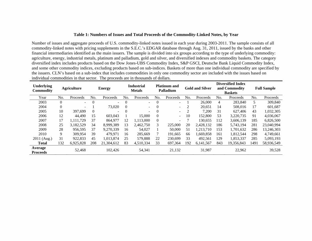
Table 1: Numbers of Issues and Total Proceeds of the Commodity-Linked Notes, by Year

Number of issues and aggregate proceeds of U.S. commodity-linked notes issued in each year during 2003-2011. The sample consists of all commodity-linked notes with pricing supplements in the S.E.C.’s EDGAR database through Aug. 31, 2011, issued by the banks and other financial intermediaries identified as the main issuers. The sample is divided into six groups according to the type of underlying commodity: agriculture, energy, industrial metals, platinum and palladium, gold and silver, and diversified indexes and commodity baskets. The category diversified index includes products based on the Dow Jones-UBS Commodity Index, S&P GSCI, Deutsche Bank Liquid Commodity Index, and some other commodity indices, excluding products based on sub-indices. Baskets of more than one individual commodity are specified by the issuers. CLN’s based on a sub-index that includes commodities in only one commodity sector are included with the issues based on individual commodities in that sector. The proceeds are in thousands of dollars.

Underlying Commodity

Agriculture Energy Industrial

Metals Platinum and

Palladium Gold and Silver

Diversified Index and Commodity

Baskets Full Sample

Year No. Proceeds No. Proceeds No. Proceeds No. Proceeds No. Proceeds No. Proceeds No. Proceeds 2003 0 - 0 - 0 - 0 - 1 26,000 4 283,840 5 309,840 2004 0 - 1 73,020 0 - 0 - 2 20,651 14 508,016 17 601,687 2005 10 397,699 0 - 0 - 0 - 2 7,200 31 627,406 43 1,032,305 2006 12 44,490 15 603,043 1 15,000 0 - 10 152,800 53 3,220,735 91 4,036,067 2007 17 1,111,729 37 864,977 12 1,113,000 0 - 7 130,655 112 3,606,139 185 6,826,500 2008 25 3,182,529 34 8,999,389 13 2,462,750 3 225,000 20 2,428,132 186 5,743,194 281 23,040,994 2009 28 956,595 37 9,270,339 16 54,027 1 50,000 51 1,213,710 153 1,701,632 286 13,246,303 2010 9 309,954 39 479,971 16 285,669 7 191,665 66 1,669,858 161 1,812,544 298 4,749,661

2011 (Aug.) 31 922,833 45 1,013,874 25 579,888 22 230,699 33 492,561 129 1,853,337 285 5,093,193 Total 132 6,925,828 208 21,304,612 83 4,510,334 33 697,364 192 6,141,567 843 19,356,843 1491 58,936,549

Average Proceeds

52,468

102,426

54,341

21,132

31,987

22,962

39,528

 

 

 

 

 

 

 

 

Table 2: Numbers of Issues and Total Proceeds of the Commodity-Linked Notes, by Issuer

Numbers of issues and aggregate proceeds of U.S. commodity-linked notes issued by each issuer during 2003-2011. The sample consists of all commodity-linked notes with pricing supplements in the S.E.C.’s EDGAR database through Aug. 31, 2011, issued by the banks and other financial intermediaries identified as the main issuers. The sample is divided into six groups according to the type of underlying commodity: agriculture, energy, industrial metals, platinum and palladium, gold and silver, and diversified indexes and commodity baskets. The category diversified index includes products based on the Dow Jones-UBS Commodity Index, S&P GSCI, Deutsche Bank Liquid Commodity Index, and other commodity indices, excluding products based on sub-indices. Baskets of more than one individual commodity are specified by the issuers. CLN’s based on a sub-index that includes commodities in only one commodity sector are included with the issues based on individual commodities in that sector. The proceeds are in thousands of dollars.

Underlying Commodity

Agriculture Energy Industrial

Metals Platinum and

Palladium Gold and Silver

Diversified Index and Commodity

Baskets Full Sample

Issuers No. Proceeds No. Proceeds No. Proceeds No. Proceeds No. Proceeds No. Proceeds No. Proceeds ABN 12 14,588 1 1,000 0 - 0 - 0 - 5 43,076 18 58,664 AIG 0 - 1 2,500 0 - 0 - 0 - 0 - 1 2,500 Bank of America 6 72,909 20 318,147 3 39,100 1 63,556 28 1,119,088 61 1,147,661 119 2,760,460 Barclays 51 2,814,935 41 6,643,574 21 1,476,929 10 219,174 39 403,770 99 4,599,251 261 16,157,633 Bear Stearns 0 - 0 - 0 - 0 - 0 - 4 27,406 4 27,406 Citigroup 2 13,183 4 22,846 7 96,000 0 - 15 173,996 18 227,201 46 533,227 Credit Suisse 0 - 2 10,193 1 4,245 0 - 1 16,055 4 10,028 8 40,521 Deutsche Bank 6 2,003,683 16 12,626,492 10 2,022,544 2 44,033 14 3,079,561 138 3,391,002 186 23,167,315 Eksportfinans 7 434,643 1 1,000 1 155,544 3 73,461 9 287,819 43 1,579,149 64 2,531,617 Goldman Sachs 3 37,060 6 56,961 1 11,001 0 - 5 92,480 40 621,537 55 819,039 HSBC 0 - 0 - 0 - 1 9,807 7 54,221 45 359,365 53 423,393 JP Morgan 8 54,696 35 298,025 15 59,433 9 43,302 22 121,812 56 407,892 145 985,160 Lehman Brothers 2 250,500 27 42,610 1 10,000 0 - 4 18,933 8 405,155 42 727,198 Merrill Lynch 6 219,698 7 241,658 0 - 0 - 8 232,795 30 1,964,673 51 2,658,824 Morgan Stanley 9 102,565 22 170,265 3 20,187 1 19,225 20 122,822 55 353,484 110 788,548 RBC 2 28,000 5 3,810 4 3,830 0 - 1 2,410 8 14,149 20 52,199 Swed. Ex. Cred. 10 649,526 8 571,797 15 561,520 2 48,776 8 202,557 128 3,069,577 171 5,103,754 UBS 8 229,843 12 293,735 1 50,000 3 175,000 9 199,906 89 1,044,866 122 1,993,349 Wachovia 0 - 0 - 0 - 0 - 2 13,342 0 - 2 13,342 Wells Fargo 0 - 0 - 0 - 1 1,030 0 - 12 91,372 13 92,402 Total 132 6,925,828 208 21,304,612 83 4,510,334 33 697,364 192 6,141,567 843 19,356,843 1491 58,936,549  

 

 

 

Table 3: Average Size of the CLN Issues, by Commodity Sector Numbers of issues and average proceeds of CLN issues for sub-samples with proceeds greater than or equal to $2 million, greater than or equal to $5 million, and greater than or equal to $10 million. The sample is divided into seven groups according to the type of underlying commodity: agriculture, energy, industrial metals, platinum and palladium, gold and silver, diversified indexes, and commodity baskets. The category diversified index includes products based on the Dow Jones-UBS Commodity Index, S&P GSCI, Deutsche Bank Liquid Commodity Index, and other commodity indices, excluding products based on sub-indices. Baskets of more than one individual commodity are specified by the issuers. CLN’s based on a sub-index that includes commodities in only one commodity sector are included with the issues based on individual commodities in that sector. Panel A shows the average proceeds for subsamples of issues satisfying the size criteria, including issues priced during the 5th through 9th business day of each month when the GSCI “rolls” from the front-month futures contracts into longer term futures contracts. Panel B excludes issues priced during the S&P GSCI roll period. The proceeds are in thousands of dollars.

Panel A: Total sample, including issues priced during the S&P GSCI roll periods

Agriculture Energy Industrial

Metals Platinum and

Palladium Gold and Silver Diversified Index

Commodity Baskets

CLN Issue Proceeds

No. Avg.

Proceeds No.

Avg. Proceeds

No. Avg.

Proceeds No.

Avg. Proceeds

No. Avg.

Proceeds No.

Avg. Proceeds

No. Avg.

Proceeds

$2 million 109 54,188 132 152,538 68 51,420 28 24,687 143 32,290 508 33,884 58 17,786

$5 million 90 64,937 91 219,770 52 66,240 22 30,712 108 41,669 402 41,961 40 24,341

$10 million 73 78,377 65 305,075 36 92,756 14 44,073 77 55,721 296 54,521 29 31,008

Panel B: Sample excluding issues priced during the S&P GSCI roll periods

Agriculture Energy Industrial

Metals Platinum and

Palladium Gold and Silver Diversified Index

Commodity Baskets

CLN Issue Proceeds

No. Avg.

Proceeds No.

Avg. Proceeds

No. Avg.

Proceeds No.

Avg. Proceeds

No. Avg.

Proceeds No.

Avg. Proceeds

No. Avg.

Proceeds

$2 million 93 59,097 107 133,876 57 59,513 28 24,687 126 30,920 391 33,056 47 17,733

$5 million 78 69,803 72 197,342 43 77,866 22 30,712 94 40,288 311 40,727 32 24,520

$10 million 63 84,727 52 270,597 32 102,413 14 44,073 70 51,880 231 52,416 21 33,820  

   

 

 

 

Table 4: Average Abnormal Returns of Underlying Commodity Futures Around the CLN Pricing Dates, Excluding Issues Priced During S&P GSCI Roll Periods

Abnormal returns of underlying commodity futures contracts around the pricing dates of the CLNs based on individual commodities and commodity baskets. CLN’s based on a commodity sub-index that includes commodities in only one commodity sector are included with the issues based on individual commodities in that sector. Issues priced during the S&P GSCI roll periods are excluded. Abnormal returns are computed relative to a benchmark given by the return predicted by a factor model, estimated using ordinary least squares and data from the 60 days immediately preceding the pricing date. The first row in each panel reports the average abnormal returns on the CLN’s underlying futures contracts around the pricing date for three different size groups. Below the returns are t-statistics for the tests of the hypothesis that the average returns are equal to zero. The next two rows present the number of positive and negative returns. The last row provides the probability that the number of positive returns equals or exceeds the number of positive returns reported in the table under the null hypothesis that the probability of a positive return is 0.5.

Panel A: Individual commodities and commodity baskets

Proceeds $2 million Proceeds $5 million Proceeds $10 million

Day 0 Day 1 Days [0,1] Day 0 Day 1

Days [0,1] Day 0 Day 1

Days [0,1]

Average abnormal return 0.22% 0.14% 0.37% 0.21% 0.19% 0.40% 0.31% 0.20% 0.51%

t-statistic 2.78 1.74 2.97 2.28 2.04 2.88 2.81 1.91 3.09

Number of returns > 0 234 239 254 169 179 193 128 130 149

Number of returns 0 224 219 204 172 162 148 124 122 103

Probability under H0 0.3371 0.1873 0.0110 0.5857 0.1931 0.0085 0.4251 0.3297 0.0022

Panel B: Individual commodities (excluding commodity baskets) Proceeds $2 million Proceeds $5 million Proceeds $10 million

Day 0 Day 1 Days [0,1] Day 0 Day 1

Days [0,1] Day 0 Day 1

Days [0,1]

Average abnormal return 0.23% 0.13% 0.37% 0.22% 0.18% 0.40% 0.33% 0.19% 0.52%

t-statistic 2.66 1.47 2.71 2.15 1.81 2.63 2.72 1.74 2.90

Number of returns > 0 208 213 224 152 160 172 117 117 136

Number of returns 0 203 198 187 157 149 137 114 114 95

Probability under H0 0.4218 0.2449 0.0378 0.6335 0.2848 0.0265 0.4477 0.4477 0.0042  

 

 

 

Table 5: Average Abnormal Returns of Underlying Commodities Around the CLN Pricing Dates by Commodity Sector, Excluding Issues Priced During GSCI Roll Periods

Abnormal returns of underlying commodity futures contracts on and around the pricing dates of the CLNs for six sub-samples of CLNs defined by commodity sector: Agriculture, Energy, Industrial Metals, Platinum and Palladium, Gold and Silver, and Commodity Baskets. CLN issues priced during the S&P GSCI roll periods are excluded. Abnormal returns are computed relative to a benchmark given by the return predicted by a factor model, estimated using ordinary least squares and data from the 60 days immediately preceding the pricing date. The first row in each panel reports the average abnormal returns on the CLN’s underlying futures contracts around the CLN pricing dates. Below the returns are t-statistics for tests of the hypothesis that the average returns are equal to zero. The next two rows present the number of positive and negative returns. The last row provides the probability that the number of positive returns equals or exceeds the number of positive returns reported in the table under the null hypothesis that the probability of a positive return is 0.5.

Panel A: Agriculture Proceeds $2 million Proceeds $5 million Proceeds $10 million Day 0 Day 1 Days [0,1] Day 0 Day 1 Days [0,1] Day 0 Day 1 Days [0,1] Average abnormal return 0.18% -0.14% 0.04% 0.24% -0.12% 0.12% 0.33% -0.28% 0.05% t-statistic 1.05 -1.02 0.20 1.25 -0.83 0.53 1.54 -1.82 0.18 Number of returns >0 51 45 44 44 37 39 37 27 33 Number of returns 0 42 48 49 34 41 39 26 36 30 Probability under H0 0.2035 0.6607 0.7330 0.1541 0.7142 0.5450 0.1037 0.8963 0.4007

Panel B: Energy Proceeds $2 million Proceeds $5 million Proceeds $10 million Day 0 Day 1 Days [0,1] Day 0 Day 1 Days [0,1] Day 0 Day 1 Days [0,1] Average abnormal return 0.31% 0.65% 0.96% 0.41% 0.72% 1.14% 0.75% 0.68% 1.43% t-statistic 1.44 2.66 2.63 1.45 2.52 2.56 2.09 1.95 2.52 Number of returns >0 51 60 62 35 40 44 28 27 31 Number of returns 0 56 47 45 37 32 28 24 25 21 Probability under H0 0.7190 0.1229 0.0608 0.6380 0.2048 0.0382 0.3389 0.4449 0.1058

Panel C: Industrial Metals Proceeds $2 million Proceeds $5 million Proceeds $10 million Day 0 Day 1 Days [0,1] Day 0 Day 1 Days [0,1] Day 0 Day 1 Days [0,1] Average abnormal return 0.50% -0.15% 0.36% 0.45% 0.19% 0.64% 0.42% 0.17% 0.59% t-statistic 1.96 -0.55 0.93 1.44 0.66 1.39 1.24 0.56 1.18 Number of returns >0 29 28 34 21 23 27 15 16 20 Number of returns 0 28 29 23 22 20 16 17 16 12 Probability under H0 0.5000 0.6043 0.0924 0.6196 0.3804 0.0631 0.7017 0.5700 0.1077

 

 

Table 5 (continued): Average Abnormal Returns of Underlying Commodities Around the CLN Pricing Dates by Commodity Sector, Excluding Issues Priced During GSCI Roll Periods

Panel D: Platinum and Palladium Proceeds $2 million Proceeds $5 million Proceeds $10 million Day 0 Day 1 Days [0,1] Day 0 Day 1 Days [0,1] Day 0 Day 1 Days [0,1] Average abnormal return 0.31% -0.22% 0.09% 0.34% -0.48% -0.13% 0.42% -0.11% 0.30% t-statistic 1.18 -0.79 0.21 1.14 -1.61 -0.28 0.96 -0.33 0.46 Number of returns >0 13 13 16 9 9 12 5 7 9 Number of returns 0 15 15 12 13 13 10 9 7 5 Probability under H0 0.7142 0.7142 0.2858 0.8569 0.8569 0.4159 0.9102 0.6047 0.2120

Panel E: Gold and Silver Proceeds $2 million Proceeds $5 million Proceeds $10 million Day 0 Day 1 Days [0,1] Day 0 Day 1 Days [0,1] Day 0 Day 1 Days [0,1]

Average abnormal return 0.07% 0.09% 0.16% -0.07% 0.15% 0.08% -

0.04% 0.33% 0.29% t-statistic 0.54 0.82 0.95 -0.57 1.16 0.43 -0.31 2.23 1.40 Number of returns >0 64 67 68 43 51 50 32 40 43 Number of returns 0 62 59 58 51 43 44 38 30 27 Probability under H0 0.4645 0.2665 0.2114 0.8233 0.2352 0.3031 0.7985 0.1410 0.0361

Panel F: Commodity Baskets Proceeds $2 million Proceeds $5 million Proceeds $10 million Day 0 Day 1 Days [0,1] Day 0 Day 1 Days [0,1] Day 0 Day 1 Days [0,1]

Average abnormal return 0.13% 0.24% 0.37% 0.15% 0.27% 0.42% 0.15% 0.28% 0.43% t-statistic 0.85 1.40 1.70 0.98 1.20 1.64 0.94 1.01 1.58 Number of returns >0 26 26 30 17 19 21 11 13 13 Number of returns 0 21 21 17 15 13 11 10 8 8 Probability under H0 0.2800 0.2800 0.0395 0.4300 0.1885 0.0551 0.5000 0.1917 0.1917

 

 

 

 

 

 

 

 

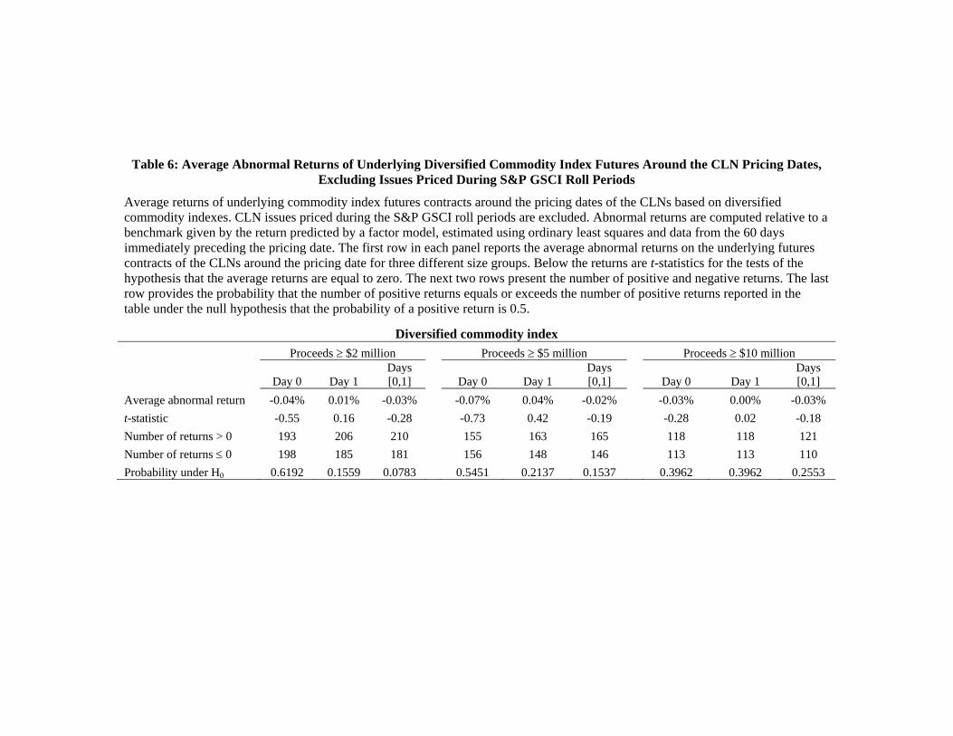
Table 6: Average Abnormal Returns of Underlying Diversified Commodity Index Futures Around the CLN Pricing Dates, Excluding Issues Priced During S&P GSCI Roll Periods

Average returns of underlying commodity index futures contracts around the pricing dates of the CLNs based on diversified commodity indexes. CLN issues priced during the S&P GSCI roll periods are excluded. Abnormal returns are computed relative to a benchmark given by the return predicted by a factor model, estimated using ordinary least squares and data from the 60 days immediately preceding the pricing date. The first row in each panel reports the average abnormal returns on the underlying futures contracts of the CLNs around the pricing date for three different size groups. Below the returns are t-statistics for the tests of the hypothesis that the average returns are equal to zero. The next two rows present the number of positive and negative returns. The last row provides the probability that the number of positive returns equals or exceeds the number of positive returns reported in the table under the null hypothesis that the probability of a positive return is 0.5.

Diversified commodity index

Proceeds $2 million Proceeds $5 million Proceeds $10 million

Day 0 Day 1 Days [0,1] Day 0 Day 1

Days [0,1] Day 0 Day 1

Days [0,1]

Average abnormal return -0.04% 0.01% -0.03% -0.07% 0.04% -0.02% -0.03% 0.00% -0.03%

t-statistic -0.55 0.16 -0.28 -0.73 0.42 -0.19 -0.28 0.02 -0.18

Number of returns > 0 193 206 210 155 163 165 118 118 121

Number of returns 0 198 185 181 156 148 146 113 113 110

Probability under H0 0.6192 0.1559 0.0783 0.5451 0.2137 0.1537 0.3962 0.3962 0.2553  

 

 

 

 

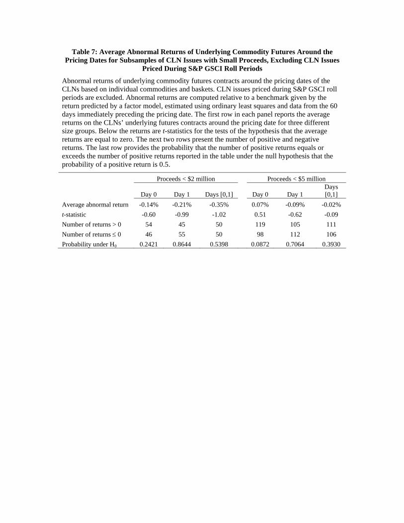
Table 7: Average Abnormal Returns of Underlying Commodity Futures Around the Pricing Dates for Subsamples of CLN Issues with Small Proceeds, Excluding CLN Issues

Priced During S&P GSCI Roll Periods

Abnormal returns of underlying commodity futures contracts around the pricing dates of the CLNs based on individual commodities and baskets. CLN issues priced during S&P GSCI roll periods are excluded. Abnormal returns are computed relative to a benchmark given by the return predicted by a factor model, estimated using ordinary least squares and data from the 60 days immediately preceding the pricing date. The first row in each panel reports the average returns on the CLNs’ underlying futures contracts around the pricing date for three different size groups. Below the returns are t-statistics for the tests of the hypothesis that the average returns are equal to zero. The next two rows present the number of positive and negative returns. The last row provides the probability that the number of positive returns equals or exceeds the number of positive returns reported in the table under the null hypothesis that the probability of a positive return is 0.5.

Proceeds < $2 million Proceeds < $5 million

Day 0 Day 1 Days [0,1] Day 0 Day 1 Days [0,1]

Average abnormal return -0.14% -0.21% -0.35% 0.07% -0.09% -0.02%

t-statistic -0.60 -0.99 -1.02 0.51 -0.62 -0.09

Number of returns > 0 54 45 50 119 105 111

Number of returns 0 46 55 50 98 112 106

Probability under H0 0.2421 0.8644 0.5398 0.0872 0.7064 0.3930  

 

 

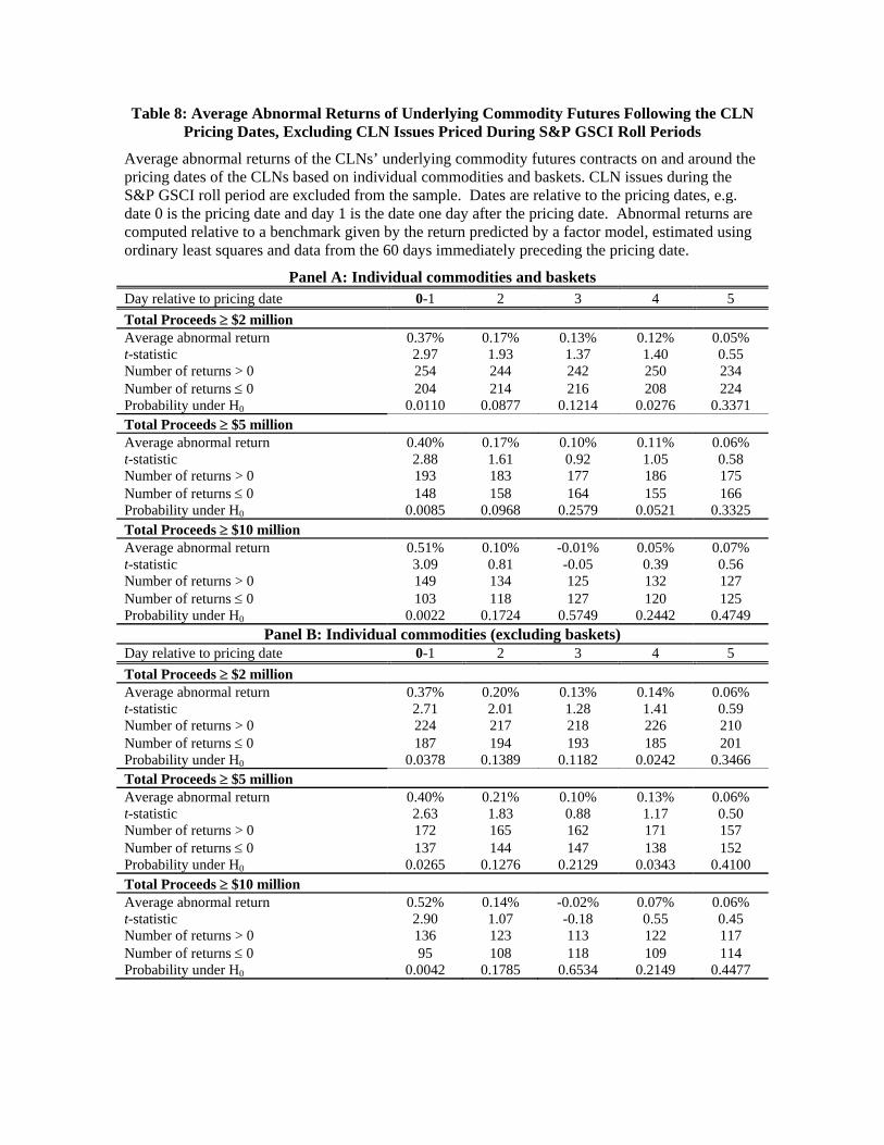
Table 8: Average Abnormal Returns of Underlying Commodity Futures Following the CLN Pricing Dates, Excluding CLN Issues Priced During S&P GSCI Roll Periods

Average abnormal returns of the CLNs’ underlying commodity futures contracts on and around the pricing dates of the CLNs based on individual commodities and baskets. CLN issues during the S&P GSCI roll period are excluded from the sample. Dates are relative to the pricing dates, e.g. date 0 is the pricing date and day 1 is the date one day after the pricing date. Abnormal returns are computed relative to a benchmark given by the return predicted by a factor model, estimated using ordinary least squares and data from the 60 days immediately preceding the pricing date.

Panel A: Individual commodities and baskets Day relative to pricing date 0-1 2 3 4 5

Total Proceeds $2 million Average abnormal return 0.37% 0.17% 0.13% 0.12% 0.05% t-statistic 2.97 1.93 1.37 1.40 0.55 Number of returns > 0 254 244 242 250 234 Number of returns 0 204 214 216 208 224 Probability under H0 0.0110 0.0877 0.1214 0.0276 0.3371 Total Proceeds $5 million Average abnormal return 0.40% 0.17% 0.10% 0.11% 0.06% t-statistic 2.88 1.61 0.92 1.05 0.58 Number of returns > 0 193 183 177 186 175 Number of returns 0 148 158 164 155 166 Probability under H0 0.0085 0.0968 0.2579 0.0521 0.3325 Total Proceeds $10 million Average abnormal return 0.51% 0.10% -0.01% 0.05% 0.07% t-statistic 3.09 0.81 -0.05 0.39 0.56 Number of returns > 0 149 134 125 132 127 Number of returns 0 103 118 127 120 125 Probability under H0 0.0022 0.1724 0.5749 0.2442 0.4749

Panel B: Individual commodities (excluding baskets) Day relative to pricing date 0-1 2 3 4 5

Total Proceeds $2 million Average abnormal return 0.37% 0.20% 0.13% 0.14% 0.06% t-statistic 2.71 2.01 1.28 1.41 0.59 Number of returns > 0 224 217 218 226 210 Number of returns 0 187 194 193 185 201 Probability under H0 0.0378 0.1389 0.1182 0.0242 0.3466 Total Proceeds $5 million Average abnormal return 0.40% 0.21% 0.10% 0.13% 0.06% t-statistic 2.63 1.83 0.88 1.17 0.50 Number of returns > 0 172 165 162 171 157 Number of returns 0 137 144 147 138 152 Probability under H0 0.0265 0.1276 0.2129 0.0343 0.4100 Total Proceeds $10 million Average abnormal return 0.52% 0.14% -0.02% 0.07% 0.06% t-statistic 2.90 1.07 -0.18 0.55 0.45 Number of returns > 0 136 123 113 122 117 Number of returns 0 95 108 118 109 114 Probability under H0 0.0042 0.1785 0.6534 0.2149 0.4477

 

 

 

 

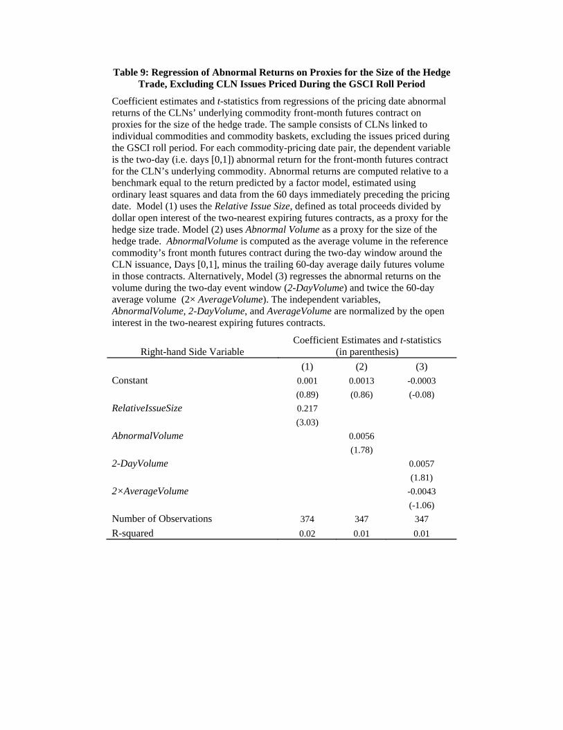
Table 9: Regression of Abnormal Returns on Proxies for the Size of the Hedge Trade, Excluding CLN Issues Priced During the GSCI Roll Period

Coefficient estimates and t-statistics from regressions of the pricing date abnormal returns of the CLNs’ underlying commodity front-month futures contract on proxies for the size of the hedge trade. The sample consists of CLNs linked to individual commodities and commodity baskets, excluding the issues priced during the GSCI roll period. For each commodity-pricing date pair, the dependent variable is the two-day (i.e. days [0,1]) abnormal return for the front-month futures contract for the CLN’s underlying commodity. Abnormal returns are computed relative to a benchmark equal to the return predicted by a factor model, estimated using ordinary least squares and data from the 60 days immediately preceding the pricing date. Model (1) uses the Relative Issue Size, defined as total proceeds divided by dollar open interest of the two-nearest expiring futures contracts, as a proxy for the hedge size trade. Model (2) uses Abnormal Volume as a proxy for the size of the hedge trade. AbnormalVolume is computed as the average volume in the reference commodity’s front month futures contract during the two-day window around the CLN issuance, Days [0,1], minus the trailing 60-day average daily futures volume in those contracts. Alternatively, Model (3) regresses the abnormal returns on the volume during the two-day event window (2-DayVolume) and twice the 60-day average volume (2× AverageVolume). The independent variables, AbnormalVolume, 2-DayVolume, and AverageVolume are normalized by the open interest in the two-nearest expiring futures contracts.

Right-hand Side Variable Coefficient Estimates and t-statistics

(in parenthesis)

   (1) (2) (3) Constant 0.001 0.0013 -0.0003

   (0.89) (0.86) (-0.08)

RelativeIssueSize 0.217

   (3.03)

AbnormalVolume 0.0056

   (1.78)

2-DayVolume 0.0057

   (1.81)

2×AverageVolume -0.0043

   (-1.06)

Number of Observations 374 347 347

R-squared 0.02 0.01 0.01  

 

 

 

 

 

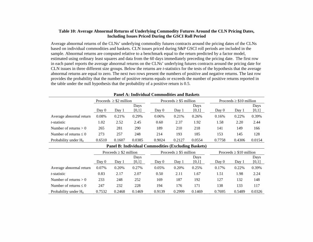
Table 10: Average Abnormal Returns of Underlying Commodity Futures Around the CLN Pricing Dates, Including Issues Priced During the GSCI Roll Period

Average abnormal returns of the CLNs’ underlying commodity futures contracts around the pricing dates of the CLNs based on individual commodities and baskets. CLN issues priced during S&P GSCI roll periods are included in the sample. Abnormal returns are computed relative to a benchmark equal to the return predicted by a factor model, estimated using ordinary least squares and data from the 60 days immediately preceding the pricing date. The first row in each panel reports the average abnormal returns on the CLNs’ underlying futures contracts around the pricing date for CLN issues in three different size groups. Below the returns are t-statistics for the tests of the hypothesis that the average abnormal returns are equal to zero. The next two rows present the numbers of positive and negative returns. The last row provides the probability that the number of positive returns equals or exceeds the number of positive returns reported in the table under the null hypothesis that the probability of a positive return is 0.5.

Panel A: Individual Commodities and Baskets

Proceeds $2 million Proceeds $5 million Proceeds $10 million

Day 0 Day 1 Days [0,1] Day 0 Day 1

Days [0,1] Day 0 Day 1

Days [0,1]

Average abnormal return 0.08% 0.21% 0.29% 0.06% 0.21% 0.26% 0.16% 0.22% 0.39%

t-statistic 1.02 2.52 2.45 0.60 2.37 1.92 1.58 2.20 2.44

Number of returns > 0 265 281 290 189 210 218 141 149 166

Number of returns 0 273 257 248 214 193 185 153 145 128

Probability under H0 0.6510 0.1607 0.0385 0.9024 0.2127 0.0554 0.7758 0.4306 0.0154

Panel B: Individual Commodities (Excluding Baskets)

Proceeds $2 million Proceeds $5 million Proceeds $10 million

Day 0 Day 1 Days [0,1] Day 0 Day 1

Days [0,1] Day 0 Day 1

Days [0,1]

Average abnormal return 0.07% 0.20% 0.27% 0.05% 0.20% 0.25% 0.17% 0.22% 0.39%

t-statistic 0.83 2.17 2.07 0.50 2.11 1.67 1.51 1.98 2.24

Number of returns > 0 233 248 252 169 187 192 127 132 148

Number of returns 0 247 232 228 194 176 171 138 133 117

Probability under H0 0.7532 0.2468 0.1469 0.9139 0.2999 0.1469 0.7695 0.5489 0.0326  

 

 

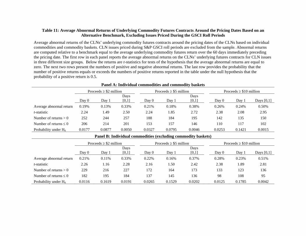
Table 11: Average Abnormal Returns of Underlying Commodity Futures Contracts Around the Pricing Dates Based on an Alternative Benchmark, Excluding Issues Priced During the GSCI Roll Periods

Average abnormal returns of the CLNs’ underlying commodity futures contracts around the pricing dates of the CLNs based on individual commodities and commodity baskets. CLN issues priced during S&P GSCI roll periods are excluded from the sample. Abnormal returns are computed relative to a benchmark equal to the average underlying commodity futures return over the 60 days immediately preceding the pricing date. The first row in each panel reports the average abnormal returns on the CLNs’ underlying futures contracts for CLN issues in three different size groups. Below the returns are t-statistics for tests of the hypothesis that the average abnormal returns are equal to zero. The next two rows present the numbers of positive and negative abnormal returns. The last row provides the probability that the number of positive returns equals or exceeds the numbers of positive returns reported in the table under the null hypothesis that the probability of a positive return is 0.5.

Panel A: Individual commodities and commodity baskets

Proceeds $2 million Proceeds $5 million Proceeds $10 million

Day 0 Day 1 Days [0,1] Day 0 Day 1

Days [0,1] Day 0 Day 1 Days [0,1]

Average abnormal return 0.19% 0.13% 0.33% 0.21% 0.18% 0.38% 0.26% 0.24% 0.50%

t-statistic 2.24 1.49 2.50 2.24 1.85 2.72 2.38 2.08 2.95

Number of returns > 0 252 244 257 188 184 195 142 135 150

Number of returns 0 206 214 201 153 157 146 110 117 102

Probability under H0 0.0177 0.0877 0.0050 0.0327 0.0795 0.0046 0.0253 0.1421 0.0015

Panel B: Individual commodities (excluding commodity baskets)

Proceeds $2 million Proceeds $5 million Proceeds $10 million

Day 0 Day 1 Days [0,1] Day 0 Day 1

Days [0,1] Day 0 Day 1 Days [0,1]

Average abnormal return 0.21% 0.11% 0.33% 0.22% 0.16% 0.37% 0.28% 0.23% 0.51%

t-statistic 2.26 1.16 2.28 2.16 1.50 2.42 2.38 1.89 2.81

Number of returns > 0 229 216 227 172 164 173 133 123 136

Number of returns 0 182 195 184 137 145 136 98 108 95

Probability under H0 0.0116 0.1619 0.0191 0.0265 0.1529 0.0202 0.0125 0.1785 0.0042