neural networks - university of london worldwide

Neural networks

A. Vella and C. Vella

CO3311

2009

Undergraduate study in Computing and related programmes

This is an extract from a subject guide for an undergraduate course offered as part of the

University of London International Programmes in Computing. Materials for these programmes

are developed by academics at Goldsmiths.

For more information, see: www.londoninternational.ac.uk

This guide was prepared for the University of London International Programmes by:

Dr Alfred D. Vella, BSc, PhD, MSc, BA, FIMA, MBCS, CEng, CMath

and

Carol A. Vella, BSc, MSc, BA, PGCert. T&L in HE, PGDip. T&L in HE.

This is one of a series of subject guides published by the University. We regret that due to pressure of work the authors are

unable to enter into any correspondence relating to, or arising from, the guide. If you have any comments on this subject

guide, favourable or unfavourable, please use the form at the back of this guide.

University of London International Programmes

Publications Office

32 Russell Square

London WC1B 5DN

United Kingdom

www.londoninternational.ac.uk

Published by: University of London

© University of London 2009

The University of London asserts copyright over all material in this subject guide except where otherwise indicated. All rights

reserved. No part of this work may be reproduced in any form, or by any means, without permission in writing from the

publisher. We make every effort to respect copyright. If you think we have inadvertently used your copyright material, please

let us know.

i

Contents

Contents

Chapter 1: Introduction ............................................................................................11.1 About this half unit...........................................................................................1

Aims .................................................................................................................1Objectives .........................................................................................................1Learning outcomes ...........................................................................................1Coursework ......................................................................................................1Essential reading ..............................................................................................2Further reading .................................................................................................2

1.2 About this guide ...............................................................................................2How to use this guide .......................................................................................3

1.3 Materials on the CD-ROM...............................................................................31.4 Recommendation on study time ......................................................................41.5 Examinations ...................................................................................................4

Advice on revising ...........................................................................................4A reminder of your learning outcomes .............................................................4

Chapter 2: Motivation for artificial neural networks ............................................5Learning outcomes ...........................................................................................5Essential reading ..............................................................................................5Further reading .................................................................................................5

2.1 Introduction ......................................................................................................52.2 Historical perspective.......................................................................................72.3 ANN Goals, tools and techniques ....................................................................72.4 Natural versus artificial neural networks .........................................................82.5 Representations of neural networks .................................................................92.6 Notation specific to this guide........................................................................ 11

A reminder of your learning outcomes ...........................................................13Chapter 3: The artificial neuron: Perceptrons .....................................................15

Learning outcomes .........................................................................................15Essential reading ............................................................................................15

3.1 Introduction: Single units ...............................................................................153.2 Units with binary inputs and step activation ..................................................163.2.1 One or two inputs ........................................................................................163.2.2 Three or more inputs ...................................................................................173.2.3 A unit as a line in the plane .........................................................................193.2.4 Drawing a line in a plane ............................................................................20

Learning activity ............................................................................................223.3 A single unit with feedback ............................................................................223.4 Single layers of units ......................................................................................24

A reminder of your learning outcomes ...........................................................24

311 Neural newtworks book.indb 1 27/10/2009 16:40:42

ii

Chapter 4: Multi-layered feed-forward networks ................................................25Learning outcomes .........................................................................................25Essential reading ............................................................................................25

4.1 Introduction ....................................................................................................254.2 Building a neural network for an arbitrary truth table ...................................254.3 More complex problems ................................................................................30

A reminder of your learning outcomes ...........................................................30Chapter 5: ANN as search ......................................................................................31

Learning outcomes .........................................................................................31Essential reading ............................................................................................31

5.1 Introduction: problem solving as search ........................................................315.2 Supervised and unsupervised learning ...........................................................325.3 Batched and unbatched learning ....................................................................325.4 ANN architecture ...........................................................................................33

A reminder of your learning outcomes ...........................................................33Chapter 6: Training networks ................................................................................35

Learning outcomes .........................................................................................35Essential reading ............................................................................................35Further reading ...............................................................................................35

6.1 Introduction ....................................................................................................356.2 Perceptron learning ........................................................................................356.3 Backpropagation networks.............................................................................36

A reminder of your learning outcomes ...........................................................39Chapter 7: Kohonen-Grossberg counterpropagation networks .........................41


7.1 Introduction ....................................................................................................417.2 The Kohonen layer .........................................................................................42

Reading...........................................................................................................45A reminder of your learning outcomes ...........................................................45

Chapter 8: Boltzmann machines ............................................................................47Learning outcomes .........................................................................................47Essential reading ............................................................................................47Further reading ...............................................................................................47

8.1 Introduction ....................................................................................................478.2 Simulated annealing in ANNs ........................................................................48



iii

Contents

Chapter 9: Hopfield nets .........................................................................................51Learning outcomes .........................................................................................51Essential reading ............................................................................................51Further reading ...............................................................................................51

9.1 Introduction ....................................................................................................519.2 Calculating transitions between states ...........................................................539.3 State transition diagrams ................................................................................549.4 Understanding Hopfield networks .................................................................559.5 Hebb’s rule .....................................................................................................569.6 The Widrow-Hoff rule ...................................................................................56


Chapter 10: Problems in ANN learning ................................................................59Learning outcomes .........................................................................................59Essential reading ............................................................................................59

10.1 Introduction ..................................................................................................5910.2 Overfitting, network paralysis and momentum ............................................59

A reminder of your learning outcomes ...........................................................61Chapter 11: Applications of neural networks .......................................................63


11.1 Introduction: The diversity of ANN applications.........................................63Learning activity ............................................................................................65A reminder of your learning outcomes ...........................................................65

Appendix A: Excel and Word-friendly notation for units ........................................67

Appendix B: Bibliography .......................................................................................69

Appendix C: Web resources .....................................................................................71

Appendix D: Coursework assignments ....................................................................73

Appendix E: Sample examination paper ..................................................................79

Appendix F: Artificial neural network projects........................................................83


iv

Notes


1

Chapter 1: Introduction

Chapter 1

Introduction

1.1 About this half unitAims

The aim of this half unit is to introduce you to the exciting topic of neural networks, which are often called artificial neural networks (ANNs) to distinguish them from natural neural networks (such as the brain). Although this is quite an old topic as far as computing subjects go, many believe that there remain important discoveries to be made – these are just waiting for the right person to come along. Perhaps that person is you!

While this half unit will not make you an expert in neural networks, it will introduce you to many of the important concepts and techniques in this area of computing, the major types of ANN and also some of the literature and other resources that are freely available on the internet.

We hope it will also encourage you to explore this area further, and perhaps to contribute to future developments or new applications.

ObjectivesThe objectives of this subject guide are to:

• enable students to understand important concepts and theories of artificial neural networks (ANNs)

• enable students to understand how ANNs can be designed and trained • enable students to calculate simple examples of ANNs • give students an appreciation of some of the limitations and

possibilities of ANNs.

Learning outcomesBy the end of this half unit, and having completed the relevant readings and activities, you should be able to:

• describe various types of ANNs • carry out simple simulations of ANNs • discuss the theory on which ANNs are based • explain how simple ANNs can be designed • explain how ANNs can be trained • discuss the limitations and possible applications of ANNs.

CourseworkCoursework will be designed to:

• encourage students to consolidate their learning by practising simulating simple neural networks by hand, by programming and/or by using readily available software, and to present their results appropriately

• encourage students to read more widely than the subject guide and set textbook and to evaluate and summarise their findings.


2

311 Neural networks

Essential readingThe set text for this half unit is Rojas, R. (1996) Neural networks: a systematic introduction. (Berlin: Springer-Verlag, 1996) [ISBN 3540605053; 978354060508]. It is available online at www.inf.fu-berlin.de/inst/ag-ki/rojas_home/documents/1996/NeuralNetworks/neuron.pdf (Last accessed June 2009.)

We agree with a review of the book on the Association for Computing Machinery’s website which says: ‘If you want a systematic and thorough overview of neural networks, need a good reference book on this subject, or are giving or taking a course on neural networks, this book is for you.’

References to Rojas will take the form r3.2.1 for Section 2.1 of Chapter 3 or rp33 for page 33 of Rojas (for example) – you should have no difficulty interpreting this. Do try to read this valuable resource – even if you are not told to do so directly. Also, if the mathematics is too much for you on first reading, it might be worth having a skim through it and returning to it again later.

Further readingComplementary resources include:

Kröse, Ben J.A. and P. Patrick van der Smagt An introduction to neural networks. (Amsterdam: University of Amsterdam, 1996). Available online at: http://math.uni.lodz.pl/~fulmanp/zajecia/nn/neuro-intro.pdf (Last accessed June 2009.)

MacKay, D.J.C. Information theory, inference and learning algorithms. (Cambridge: Cambridge University Press, 2005) [ISBN-13: 9780521642989; ISBN-10: 0521642981]. Available online at: www.inference.phy.cam.ac.uk/mackay/itila/book.html) (Last accessed June 2009.)

1.2 About this guideThis guide sets out some of the important concepts in neural networks, and guides you through important further reading from the set text Rojas (1996).

Many people working with ANNs like to take shortcuts by using mathematical arguments and proofs. Do not be put off by these. There are some formulae that you need to remember but the derivations are not part of our study – read them ‘lightly’.

This guide is written in a fairly informal style. Some use of formal notation is necessary, but this is introduced as appropriate. Some mathematical ideas are also introduced, but we have tried to avoid too much maths for maths’ sake (for the benefit of students who may not have much mathematical background). An understanding of mathematics equivalent to the Level 1 mathematics courses for the Computing and Other Related Subjects and Mathematics, Statistics and Computing degree programmes is assumed. In particular, simple algebraic manipulation of vectors and matrices is important, and you may like to refresh your memory of these topics.

For those students interested in exploring the mathematics in more detail, we indicate the sections in the set text where a fuller account can be found.

This guide is not intended to be a comprehensive account or a textbook, but to introduce you to some important concepts and to help you explore


3

Chapter 1: Introduction

these in more depth by guided reading of the set text and selected internet resources.

You may also need to research particular topics in more depth as part of the coursework. When doing so, you should carefully evaluate online resources in terms of their relevance, timeliness, objectivity and authoritativeness to make sure the information they contain is reliable and useful. Remember too that online resources must be referenced just as carefully as print resources.

How to use this guideEach chapter of this guide starts with:

• a list of learning outcomes • a list of essential reading • a list of further reading where appropriate.

The learning outcomes should be used as a guide for your skills development. Use them to focus your learning.

The essential reading aims to act as a warning of what reading you will be asked to do as you study the material of the chapter. You are advised to make sure that the material is easily accessed but do not read the material until told to do so in the text. Of course we encourage you to read the ‘rest’ of the material when you have time.

It is good practice to review the material again once you have worked through the chapter and at least once again when you are revising for the examination.

Further reading, if any is given, is best studied after working through the chapter unless otherwise directed in the text. After studying a chapter it is also worth using Google or another search engine to see what other information on the topic is available. Lots of material finds its way onto the web each week.

1.3 Materials on the CD-ROMAccompanying this guide is a CD-ROM that contains Excel spreadsheets that implement some of the models that you will study. The use of the spreadsheets is explained in Section D of the document on the CD-ROM entitled Guide to the CD-ROM. This document also includes:

• an introduction to the CD-ROM (Section A) • sample answers to the exercises in the guide (where appropriate)

(Section B) • a note on simulating neural networks (Section C) • a section on writing up coursework (Section E) • a section on examinations, including advice on answering Sample

examination questions (Section F) • a section on evaluating ANNs (Section G) • a list of some freely available data sets that you might like to use in

your work (Section H) • a copy of the half unit’s syllabus (Section I) • a list of recommended readings (Section J) • a list of useful resources (Section K).

The best way of using the CD-ROM is to become familiar with its contents and then to consult this material when advised to by this text, or when you feel confident with its contents, or when you think that it might be useful.


4

311 Neural networks

1.4 Recommendation on study time As p.35 of the CIS and CC Handbook [available online at http://www.londonexternal.ac.uk/current_students/general_resources/handbooks/cis_cc/ciscc_comphb.pdf] says: ‘To be able to gain the most benefit from the programme, and hence do well in examinations, it is likely that you will have to spend at least 250 hours studying for each full unit, although you are likely to benefit from spending up to twice this time.’ So we would expect you to spend between 125 and 250 hours in total on study in order to do justice to this half unit subject.

1.5 Examinations Advice on revising

Experience of teaching many hundreds of students suggests that two very important strategies for success when studying neural networks are:

1. Read widely.2. Practise by doing lots of examples.This guide will lead you through the important topics in artificial neural networks and will give you the most important results. However, we learn best when we become familiar with a topic and this familiarity is aided by being presented with many views of the same topic. That is why we have tried to find many sources on the web. Some of the books that we have recommended to you are also freely available on the web. You should use them!

Neutral networks is a practical topic in which the computer is made to perform many, many calculations. However, it is only by doing calculations by hand on some easy examples that we can become confident that we understand what we are asking the computer to do.

The examination format has not changed with the revision of this guide. You are expected to answer four questions out of six in 2 hours 15 minutes. The CD-ROM contains a document, entitled Guide to the CD-ROM, which contains advice on answering the examination questions (see Section F).

Important: The information and advice given in the above section are based on the examination structure used at the time this guide was written. We strongly advise you to always check the current Regulations for relevant information about the examination. You should also carefully check the rubric/instructions on the paper you actually sit and follow those instructions.

A reminder of your learning outcomesBy the end of this half unit, and having completed the relevant readings and activities, you should be able to:

• describe various types of ANNs • carry out simple simulations of ANNs • discuss the theory on which ANNs are based • explain how simple ANNs can be designed • explain how ANNs can be trained • discuss the limitations and possible applications of ANNs.


5

Chapter 2: Motivation for artificial neural networks

Chapter 2

Motivation for artificial neural networks

Learning outcomesBy the end of this chapter, and having completed the relevant readings and activities, you should be able to:

• explain the motivations for studying ANNs • explain the basic structure, working and organisation of biological

neurons • interpret diagrams of units such as Figure 2.2b and diagrams containing

many connected units • define the terms: unit, weight, activation function, activation, net,

threshold, bias, fires and architecture as they relate to ANNs. • understand and explain the notational equivalence of: ?a, ?b…; input1,

input2… and x1, x2… • understand and explain the use of the following symbols: wiu, wuv, Σ,

A(), au, T(<0,0,1).

Essential readingRojas 1.1, 1.2 and 1.3. However, do not read these sections until prompted to do so by the text.

Farabee, M. (2009) The nervous system. Available online at: www.estrellamountain.edu/faculty/farabee/biobk/BioBookNERV.html (Last accessed June 2009.)

Clabaugh, C., D. Myszewski and J. Pang (2009) Neural networks. Available online at: http://cse.stanford.edu/class/sophomore-college/projects-00/neural-networks/Files/presentation.html (Last accessed June 2009.)

Carnegie Mellon (2009) Center for the Neural Basis of Cognition. Available online at: www.cnbc.cmu.edu (Last accessed June 2009.)

Further readingKleinberg, J. and C. Papadimitriou Computability and Complexity in Computer Science: Reflections on the Field, Reflections from the Field. (Washington, D.C.: National Academies Press, 2004) Available online at: www.cs.cornell.edu/home/kleinber/cstb-turing.pdf (Last accessed August 2009.)

2.1 IntroductionWell before the era of computing machines, people wondered about the nature of intelligence and whether it would be possible to make machines that displayed ‘intelligence’. It is from these questions that our subject emerges in the 1940s.

As its title indicates, this subject guide is about ‘neural networks’ or NNs: that is, networks of ‘neurons’. Although much of the time we will be considering networks, the choice of the name ‘neuron’ which was made many years ago, is a little unfortunate – although well meaning. Like many in the field we prefer to call the items in our networks ‘units’ and to use the acronym ANN to emphasise that these are networks of ‘artificial neurons’.


6

311 Neural networks

Neural networks are not a new idea and in fact their history can be traced back to 1943, long before that of Artificial Intelligence (or AI, a term which was coined around 1952). Alan Turing had spent much time thinking about computation and what could – and what could not – be computed by ‘automatic machines’; which (at least in his early work) he probably thought of as humans obeying written step-by-step instructions. Later he spent much time during the Second World War attempting to make machines do tasks with which the brightest minds in the land were having difficulty! As humans were the ‘systems’ where intelligence, at least as it was then understood, was most evident, it seems natural that Turing should wonder if mankind’s thinking capabilities could be simulated on the new breed of machines that were being built after the war. His thoughts therefore turned to making machines appear more intelligent – that is, he thought about what has now come to be called Artificial Intelligence. Artificial neural networks can be thought of as one of many ‘biologically inspired’ attempts at AI.

To understand fully the motivation for ANNs, we need to look at the motivation for Artificial Intelligence itself.

There are three equally valid reasons for studying Artificial Intelligence and thus ANNs:

1. To make better machines. Turing was interested in making machines more useful – this is what

one might call the ‘engineer’s rationale’. After all, he had spent time during the Second World War trying to decipher intercepted messages with the aid of the immediate precursors of computers.

2. To model human/animal intelligence. Another, equally valid reason is an attempt to understand better the

ways that the intelligent behaviour of humans might arise from a processing point of view – this might be termed the ‘psychologist’s rationale’. Turing showed his interest in this study – possibly as a means of informing attempts at 1. above. Understanding this process might allow us to help humans with difficulties and also might feed back to goal 1. above.

3. To explore the idea of intelligence. Finally, we might broaden our view of intelligence to include intelligent

behaviour of other primates, or more broadly other mammals – perhaps whales and dolphins, among others. Going beyond this to the extreme, we might ask ‘what forms could intelligence have?’ – this might be the ‘philosopher’s rationale’. There is absolutely no reason why intelligence cannot exist in forms almost unrecognisable to us. In fact, there is a whole industry of people asking if machines could have mind, consciousness, etc. You might meet this if you study AI.

Once you have studied this subject we hope that you will have at least some idea of how artificial neural networks might go some way towards each of these three goals, but much of the guide concentrates just on Goal 1. above – making better machines.


7


2.2 Historical perspectiveTuring had shown that it was possible to design ‘universal calculating machines’; that is, machines which could, at least in principle, calculate anything that was theoretically computable. For more on what is or is not computable see Kleinberg and Papadimitriou (2004) and the references that they cite. It is also worth reading Rojas sections 1.1.2 and 1.1.3 at this stage.

However, Turing knew that there was a big difference between being able to do something ‘in principle’ and actually doing it. He had made many hand simulations of his ‘universal machines’ and from this experience understood that ‘programming’ them could be (at the very least) extremely tedious.

So Turing thought about the possibility of machines that could be taught to do things by experience rather than by instruction. It is this ability that sets neural networks apart from many other branches of computing.

We can summarise the goals of Artificial Neural Network research as:

The study of networks of simple processing elements and of what can and cannot be done with them especially in the context of the three goals 1., 2. and 3. mentioned above.

However, we do not have the space (and you do not have the time) to consider in detail all three goals!

2.3 ANN Goals, tools and techniquesThe last section included a one-sentence summary of the goals of our study (artificial neural networks) but we need to focus a little more.

Despite its age, the science of artificial neural networks continues to progress, with new techniques and applications being developed all the time. This is both a strength and a weakness of the subject. It is a strength because there continues to be a healthy interest among ‘amateurs’ and a weakness because it is difficult to settle upon those fundamental principles of the subject that are likely to be around in (say) 50 years’ time. Instead we are forced to give a snapshot of a few of the many types of systems that go under the name ‘artificial neural network’ and try to give some principles that underlie at least some of them.

A key issue in the use of computers to solve problems is the presentation of potential or candidate solutions to those problems in a form that is amenable to efficient representation on a computer. By manipulating such candidate solutions it is hoped that we can find one that will serve our purpose.

Artificial neural networks (ANNs) are representations of computing problems in the form of one or more networks of processing elements, historically called ‘neurons’ – hence the name ‘neural network’. However, nowadays the term unit is preferred to distance these from the biological neurons in our brains. As our understanding of the latter improves, we see just how different the biological neuron is from the artificial units in our networks.

Different problems have different representations, but some representations are powerful enough to represent all problems – known as universal representations. Whether they do this efficiently or not is another issue.


8

311 Neural networks

So, for example, although we know that almost any general purpose programming language will do for any computing problem, we also know that some problems lend themselves well to particular languages. If you have studied a range of languages (declarative, functional, procedural and object oriented) such as Prolog, SML, Pascal and Java or similar languages, you will know what we mean.

In general, the types of problem that we try to solve using ANNs are those that are very difficult to solve otherwise. This is what makes it worthwhile putting the effort into finding new ways of solving the problems – there are no real alternatives known.

Those used to programming will know that finding a ‘good’ way of representing our problem is a key step in its solution. Once we have found such a representation we use this with a set of data structures and algorithms – possibly in the form of objects, their members and their methods.

However, some problems, although reasonably easy to state (and represent), are very difficult to solve because we cannot find a suitable algorithm. When finding algorithms proves too difficult, we may take another line of attack: perhaps we can represent our problems as search problems where we might use some well known search techniques. We will see later how the use of ANNs can be thought of as a type of search.

The ways in which the Artificial Intelligence community has tackled these problems can be classified into ‘Knowledge Rich Strategies’ and ‘Knowledge Poor Strategies’. In the Knowledge Rich strategies, some of which you may learn about in the half unit on AI, we build into our computer models as much knowledge about the problem domain as we can. The language used in Expert Systems, for example, is that of experts. In contrast with this, the knowledge poor strategies concentrate on general techniques that do not depend upon the particular problem at hand. This enables us to refine the techniques in the hope and expectation that they are applicable widely rather than to a narrow set of applications.

There is much competition between the camps of researchers who prefer one strategy type over the other and sometimes this rivalry has had some negative effects on progress. However, it is not our intention to say any more about that here.

2.4 Natural versus artificial neural networksThe biology of physical neurons within the nervous system provided the original inspiration for artificial neural networks. In fact, ANNs were originally an attempt to explain how our neurons worked. Of course, once the power of computing with ANNs was appreciated, a large section of the neural network community moved on to investigate modifications of the original neural models in order to optimise their computational possibilities, with little or no attempt at preserving any plausible connection with natural neurons. In fact, there was very little plausibility even in the first neural networks.

Natural neurons are activated, generating an electrical signal, if the received stimulus is above a certain threshold. This is sometimes referred to as the neuron ‘firing’. The electrical signal is transmitted along the neuron, and may be passed on to other neurons which are connected, and these in turn may either ‘fire’ or not, depending on whether the signal received is above the threshold of the receiving neuron.


9


A neuron is either activated, or it is not: there are no partial activations.

It is easy to see that a neuron activating or not activating can be modelled within a binary system, with 1 representing activation and 0 representing non-activation. You may have noticed that we have used ‘activation’ and ‘non-activation’ above. We did this to avoid later confusion, because unfortunately, within artificial neural networks, the term ‘firing’ is applied whenever the calculation takes place whether the outcome is 1 or 0. So don’t be caught out!

The threshold (or –bias) idea is also readily modelled within artificial neural networks.

Artificial neural networks do not approach the complexity of natural nervous systems, but can still be usefully applied to solve certain classes of problem. On this topic it would be worth reading Rojas section 1.1.1.

Exercise 1

At this stage it is worth you looking at a couple of useful resources that are available on the web.

A website that has a good summary of the biological aspects of nerves is Farabee (2009). Navigate to it and read up to ‘Divisions of the Nervous System’.

Next, visit Stanford University’s website Clabaugh (2009) which has a short tutorial on ANNs. Have a quick look at this now – and maybe again after you have studied all of this half unit.

While reading these sites, make brief notes about the main properties of natural neurons.

We will leave it up to you to decide just how alike natural and artificial neural networks are – but we might ask you for your opinion, with reasoning, as part of an examination or assignment question.

The University of Pittsburgh and Carnegie Mellon have set up the ‘Center for the Neural Basis of Cognition: Integrating the sciences of mind and brain’. This site Carnegie Mellon (2009) is definitely worth looking at.

Reading

Now read Rojas Section 1.2, which covers much of this topic in more detail.

2.5 Representations of neural networksAs the name ‘neural network’ implies, we are studying the potential of networks of neurons – so a good place to start might be with an idea of what ‘a neuron’ might be. We do, however choose to use the term unit rather than neuron. At its simplest we have an ‘object’ with inputs and outputs and which processes the inputs to produce these outputs. This model is much like that of the computer itself.

A neural network is a network of ‘simple’ computing units – in a sense that is all that they have in common. Assuming that you do the reading and web work recommended, you will have met many different but by no means all neural network types after studying this half unit.

Some authors use a rectangular box, of no particular size to represent a unit. Figure 2.1 shows such a box.


10

311 Neural networks

We will use the letter u to denote a particular unit. Three lines meet the box in the figure and these lines, or edges, represent a means of this unit’s communication with other units and with the outside world. Communication often takes the form of an integer or real number being passed, although sometimes we think of other forms of message. Some units have directed edges: that is, the messages (sometimes integers or sometimes real numbers) go just one way, while other types of unit can have two-way edges. The unit in the figure has one edge going in, one going out and one bidirectional edge.

Each incoming edge has a numeric weight (w say), associated with it. This may be an integer or it may be a real value. We imagine an input being sent along the edge and this input is ‘magnified’ or amplified by the weight so that an input of x arrives as w*x at the node. Most of the time we draw the diagrams so that messages go from left to right but there is no requirement for this convention and sometimes we may break it. Edges are named by their start and end unit (if they have them) and we often use the same notation for edges and their associated weights. Thus an edge going from unit u to unit v will have weight wuv. There is no significance placed upon the length of the edges and although we might later say that the diagram shows a unit, we must always remember that this is just a representation for humans!

In an ANN, besides the messages that are passed between units, we often have messages coming from outside along edges with weights wiu signifying from input i to unit u. In this guide we use a special notation for inputs. Instead of following most authors and labelling them input0, input1, … etc. or something similar, we believe that it is clearer if we use ?a, ?b, etc. for the first, second etc… inputs. However, following other authors we might sometimes use x1, x2… or even something else if this makes things clearer.

Figure 2.1: A common representation of a unit.

Once the magnified inputs arrive at the unit, it performs a calculation on these. This calculation often has two parts. For historic reasons we call the result of the first part the net of the unit. The second part of the calculation then works on the unit’s value of net to produce the unit’s activation a.

For the first part of the calculation, the most common units add the weighted inputs to form a sum which is the value of net. We will use the symbol Σ for net in such cases. So it is this sum that is passed through the activation function, A(), to produce the output which we represent using the letter a = A(Σ). There are many functions that have been used as activation functions, and we shall meet a few.

In general, there may be any number of input edges and any number of output edges. However, while the values input can be different, there can only be one value of output, although it can exit on many arrows. The output or activation of unit u is labelled au.


11


2.6 Notation specific to this guideWhile you will see lots of variations on the diagram above during your reading, some with round ‘boxes’ for example, we do not find them so informative. One of the frustrating aspects of working in neural networks is the plethora of notations used. It sometimes seems as if authors do not take the trouble to find out what others have done and just invent their own notation. It may be that with computer power becoming readily available just as neural networks became more widely explored, the notation has not yet had time to settle properly.

Unfortunately, we feel the need to add to this plethora of notation – for a good reason – that of the ease with which we can communicate with our readers here in this guide and more importantly in coursework and examinations.

For learning how single units work, it is good to implement them as spreadsheet cells. To help you to see how this might work, we introduce in this section a notation that is useful for networks with just a few units. The notation is not standard but is much easier to wordprocess than any other that we have seen.

This notation for a unit is given in Figure 2.2a and Figure 2.2b. It is not as useful though when there are lots (more than 10 say) of units.

Figure 2.2a shows that we have three inputs. The first is fixed and is just a notational convenience allowing for the bias. We use bias in our calculations: it is a property of a unit that may be given or learnt. The other inputs ?a and ?b will receive values either from another unit or from outside the neural net. We have question marks for the weights as they are not given values in this diagram. Different types of unit will have different parameters so this is just a typical one. We will discuss the use of the learning rate later when we cover training. Net represents the first of two calculations that the unit does on its inputs. The Σ indicates that it forms the sum of its weighted inputs. In this case we write:

netu = biasu + ?a wau + ?b wbu

The second calculation takes netu (which is Σu in this case) and produces a value for the activation au of the unit. One of the simplest activation functions is the step or threshold function:

A(Σu) = [if Σu ≥ 0 then 1 else 0]

When the activation function is of this form we write A(Σ) = T(<0,0,1) which stands for: au = If net < 0 then 0 else 1. That is if the value of net is less than zero the activation is 0 otherwise the activation is 1. This is called a threshold function and the unit a ‘threshold unit’ because of this. This notation for threshold relates to the way that it would be implemented in Excel, for example. Note that T(<0,0,1) is the same as T(≥0, 1, 0) but the former is often easier to write in a wordprocessor).

The name bias comes from the fact that it biases the value of net.

Inputs Weights Parameters Form Value

1 bias Learning rate η ??

?a ? Net Σ ??

?b ? Activation T(<0,0,1) ??

Figure 2.2a: A skeleton of a unit with ? showing items that need filling in.


12

311 Neural networks


1 –0.1 Learning rate η 0.15

–1 0.3 Net Σ –0.65

–1 0.25 Activation T(<0,0,1) 0

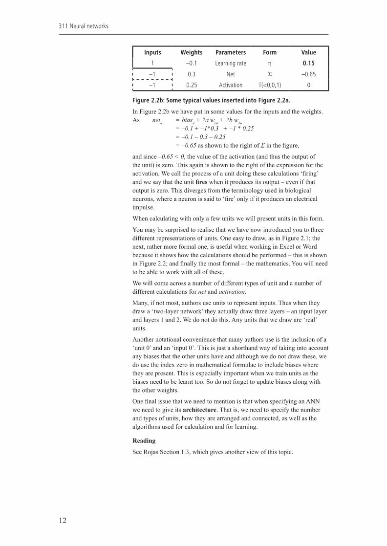
Figure 2.2b: Some typical values inserted into Figure 2.2a.

In Figure 2.2b we have put in some values for the inputs and the weights. As netu = biasu + ?a wau + ?b wbu

= –0.1 + –1*0.3 + –1 * 0.25 = –0.1 – 0.3 – 0.25 = –0.65 as shown to the right of Σ in the figure,

and since –0.65 < 0, the value of the activation (and thus the output of the unit) is zero. This again is shown to the right of the expression for the activation. We call the process of a unit doing these calculations ‘firing’ and we say that the unit fires when it produces its output – even if that output is zero. This diverges from the terminology used in biological neurons, where a neuron is said to ‘fire’ only if it produces an electrical impulse.

When calculating with only a few units we will present units in this form.

You may be surprised to realise that we have now introduced you to three different representations of units. One easy to draw, as in Figure 2.1; the next, rather more formal one, is useful when working in Excel or Word because it shows how the calculations should be performed – this is shown in Figure 2.2; and finally the most formal – the mathematics. You will need to be able to work with all of these.

We will come across a number of different types of unit and a number of different calculations for net and activation.

Many, if not most, authors use units to represent inputs. Thus when they draw a ‘two-layer network’ they actually draw three layers – an input layer and layers 1 and 2. We do not do this. Any units that we draw are ‘real’ units.

Another notational convenience that many authors use is the inclusion of a ‘unit 0’ and an ‘input 0’. This is just a shorthand way of taking into account any biases that the other units have and although we do not draw these, we do use the index zero in mathematical formulae to include biases where they are present. This is especially important when we train units as the biases need to be learnt too. So do not forget to update biases along with the other weights.

One final issue that we need to mention is that when specifying an ANN we need to give its architecture. That is, we need to specify the number and types of units, how they are arranged and connected, as well as the algorithms used for calculation and for learning.

Reading

See Rojas Section 1.3, which gives another view of this topic.


13


A reminder of your learning outcomesBy the end of this chapter, and having completed the relevant readings and activities, you should be able to:

• explain the motivations for studying ANNs • explain the basic structure, working and organisation of biological

neurons • interpret diagrams of units such as Figure 2.2b and diagrams containing

many connected units • define the terms: unit, weight, activation function, activation, net,

threshold, bias, fires and architecture as they relate to ANNs • understand and explain the notational equivalence of: ?a, ?b…; input1,

input2… and x1, x2… • understand and explain the use of the following symbols: wiu, wuv, Σ,

A(), au, T(<0,0,1).


14

311 Neural networks

Notes


15

Chapter 3: The artificial neuron: Perceptrons

Chapter 3

The artificial neuron: Perceptrons

Learning outcomesBy the end of this chapter, and having completed the relevant readings and activities, you should be able to:

• describe the architecture of the ANN that we call a Perceptron • carry out simple hand simulations of Perceptrons • manipulate the equations defining the behaviour of Perceptrons with

step activations • explain how Perceptrons can be thought of as modelling lines in the

plan • explain how simple Perceptrons (such as those implementing a NOT,

AND, NAND and OR gates) can be designed • discuss the limitations and possible applications of Perceptrons • understand the behaviour of single threshold units with feedback • understand the use of a single layer of Perceptrons to divide a plane

into parts • define the terms: threshold units, step units, step activation,

extended truth table, clamped, threshold, bipolar activation and recurrent.

Essential readingRojas, Chapter 3.

3.1 Introduction: Single unitsIn this chapter we will walk you slowly through some very simple ANNs consisting of just one simple unit. However, as we will see, even a single unit can be very powerful (although later we will see that one unit may often not be powerful enough). Following other authors we use the term ‘Perceptron’ for a single unit, giving its details when necessary. Historically, a Perceptron was a particular type of unit but we prefer to follow the common usage.

Units with just this simple step activation function are surprisingly powerful when combined as we shall soon see, but for now let us see what a lone unit can do!

One of the main problems that we will repeatedly come across during our studies is that of knowing what a given ANN actually does. Another problem is the ‘inverse’ of this – being able to build a network to do what we want it to do. We shall see that in a few cases this is no problem but in the majority of circumstances both of these are very difficult.


16

311 Neural networks

3.2 Units with binary inputs and step activation3.2.1 One or two inputs

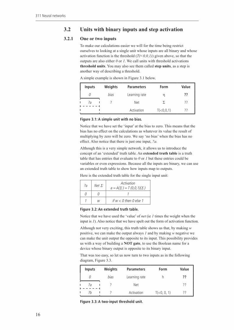
To make our calculations easier we will for the time being restrict ourselves to looking at a single unit whose inputs are all binary and whose activation function is the threshold (T(<0,0,1)) given above, so that the outputs are also either 0 or 1. We call units with threshold activations threshold units. You may also see them called step units, as a step is another way of describing a threshold.

A simple example is shown in Figure 3.1 below.


0 bias Learning rate η ??

?a ? Net Σ ??

Activation T(<0,0,1) ??

Figure 3.1: A simple unit with no bias.

Notice that we have set the ‘input’ at the bias to zero. This means that the bias has no effect on the calculations as whatever its value the result of multiplying by zero will be zero. We say ‘no bias’ when the bias has no effect. Also notice that there is just one input, ?a.

Although this is a very simple network, it allows us to introduce the concept of an ‘extended’ truth table. An extended truth table is a truth table that has entries that evaluate to 0 or 1 but these entries could be variables or even expressions. Because all the inputs are binary, we can use an extended truth table to show how inputs map to outputs.

Here is the extended truth table for the single input unit:

?a Net Σ Activationa = A(Σ ) = T (0,0,1)(Σ )

0 0 1

1 w if w < 0 then 0 else 1

Figure 3.2: An extended truth table.

Notice that we have used the ‘value’ of net (ie 1 times the weight when the input is 1). Also notice that we have spelt out the form of activation function.

Although not very exciting, this truth table shows us that, by making w positive, we can make the output always 1 and by making w negative we can make the unit output the opposite to its input. This possibility provides us with a way of building a NOT gate, to use the Boolean name for a device whose binary output is opposite to its binary input.

That was too easy, so let us now turn to two inputs as in the following diagram, Figure 3.3.


0 bias Learning rate h ??

?a ? Net Σ ??

?b ? Activation T(<0, 0, 1) ??

Figure 3.3: A two-input threshold unit.


17


Again drawing an extended truth table:

?a ?b net S Activation a = A(net)

0 0 0 1

0 1 wb if wb < 0 then 0 else 1

1 0 wa if wa < 0 then 0 else 1

1 1 wa + wb if wa + wb < 0 then 0 else 1

Figure 3.4: An extended truth table for the unit of Figure 3.3.

As you can see things are beginning to get complicated!

Exercise 2

a. Rewrite the table in Figure 3.4 using values (1, 1), (1, –1), (–1, 1) and (–1, –1) for (wa, wb).

b. Rewrite the table in Figure 3.4 using values (0, 1) and (1, 0) for (wa, wb).c. Do you recognise any of the resulting truth tables?Comment: One thing that is worth noting here is that if a weight is zero, then the node’s behaviour is independent of the corresponding input.

3.2.2 Three or more inputsIt is important that you have some facility with working out the outputs, given inputs and weights (examination questions often ask you to do this), so let us look at some more examples. The diagram below represents a unit with three or more inputs. The ‘dotted’ input ‘…’ represents 0 or more edges, allowing for an unspecified number of extra inputs.


1 bias Learning rate η 0.15

?a ? Net Σ ??

?b ? Activation T(<0,0,1) ??

… … … ... …

?N ?

Figure 3.5: An N input threshold unit.

We use capital N for the number of inputs. When we introduced the notation of the Figures, we said that it is often useful to add to the external inputs a special ‘input’ which is fixed at the value 1. We called the weight associated with this input the bias of the unit and now we are including it in the discussion. Previously we set the input to 0 but now it is clamped, that is fixed at 1. Notice that the bias does not count in the N inputs – one often finds it thought of as input 0 but, unfortunately, it is also called input N+1 by some authors.

Although dealing with such units will in general require a computer to keep track of net and activation, we will look to see if we say something about the output if the values of all but one of the weights are the same. Let us call the value of the common weight w.

In this case the value of net is the value of bias plus w times the sum of the other inputs. We can write this as:

net = bias + wΣ1N ?i


18

311 Neural networks

Here we have used ?i to denote the ith input – ? reminding us that it is an input.

The equation shows that bias indeed acts as a bias by giving the rest of the sum a head start.

To make life a little more complicated the bias, or at least an equivalent of it, has again for historical reasons, been given another name, threshold, or rather bias is ‘minus threshold’.

Suppose that we put this sum into the step activation function. We get:

a = [if (bias + wΣ1N ?i ) < 0 then 0 else 1]

This is, of course the same as saying:

a = [if wΣ1N ?i < -bias then 0 else 1]

Now we can see that –bias is acting as a (variable) threshold that the rest of the sum must equal or exceed before the output can become 1. When you read around the subject you will see threshold being mentioned, and you now know that this is just minus the bias, which in turn is the name of a weight connected to an input that is always 1.

Before we move on, let us look at what we can make with units of the type where

net = bias + wΣ1N ?i

To see what we can do let us simplify the equation a little by using the symbol M to represent the number of inputs with value 1. Also if we let bias be any real number, rather than just a whole number, then we can write our equation as:

net = bias + wM

We have been able to do this because the inputs are either 0 or 1 and all the weights are the same.

Remember that the activation is 1 if net is greater than or equal to zero, so we can write the condition for our unit to have activation 1 as:

net = bias + wM ≥ 0

or as

M ≥ -bias/w and bias ≥ -wM

These formulae give us a means of designing units which, in order to output a 1 on firing:

a. require all inputs to be a 1 (that is an AND gate) by setting w = 1 and bias = –N (the number of inputs)

b. require at least one input to be 1, by setting w = 1 and bias = –1 (this is an inclusive OR gate)

c. require at least a certain number of inputs to be 1, again setting w = 1 and bias = – the number of inputs that we want to be on. This represents a sort of ‘voting’ circuit

d. require at most M inputs to be 1 by setting w = –1 and bias = Me. require at least one of the inputs not to be 1 by setting w = –1 and bias

= N – 1 (this is the NAND gate).You can see that just by adjusting the weights (including the bias) we can design a number of useful units. In fact we know from Boolean algebra that by combining a number of NAND gates (e. above) we can make any Boolean function that we want.


19


This last result might suggest that there is nothing else to do – but that would be an incorrect conclusion. All that it implies is that we can build an ANN to compute any ‘computable function’ so that they correspond to universal computing devices. Finding the required weights is another, much harder, question. We will see how weight can be found by the use of learning algorithms that train the networks.

3.2.3 A unit as a line in the planeLet us now turn to the limitations of single units of this type, where we no longer insist that the weights are the same. Weights, inputs and bias are now arbitrary real numbers. We are going to do this by giving another way of looking at the calculation implied by the equation:

a = [if (bias + Σ1N w i ?i ) < 0 then 0 else 1]

Note that wi ?i above stands for weight wi times input ?i. The argument, though not the diagrams of lines in the plane below, works with any number of inputs – that is values for N, but to make our diagrams easy to imagine and draw we will take it to be just 2. Instead of ?a and ?b we shall use the letters x and y – for reasons that you will soon see. We will use v and w for the weights corresponding to x and y respectively.

With this notation our equation becomes:

a = if (bias + vx + wy) < 0 then 0 else 1

From co-ordinate geometry we may know that the inequality (bias + vx + wy) < 0 represents a ‘half plane’ determined by the line (bias + vx + wy) = 0 and the sign of bias. For an easy ‘trick’ to find out which side of the line corresponds to an activation of 1, just substitute x = 0 and y = 0 into the equation. This gives the activation at the origin which turns out to be the same as the bias. So if the bias is < 0, the origin has activation of zero and if the bias is positive the activation at the origin is 1. (This link with co-ordinate geometry is the reason we are using x and y notation here, as you have probably realised.)

Exercise 3

On a single piece of graph paper plot the line: (bias + vx + wy) = 0 for the values of bias, v and w given in the following table:

bias v w

0 0 0

0 0 1

0 1 0

0 1 1

1 0 0

1 0 1

1 1 0

1 1 1

Figure 3.6: Simple parameters for showing parameters of two-input threshold units.

For each line, mark which half plane represents the activation being 1 – you might like to use different colours for the lines to help keep tabs on which half plane belongs to which line.


20

311 Neural networks

Of course you could use Excel or another package to draw the lines for you – but you cannot do this in an examination so it is important to practise doing it by hand too.

We have included a simple line drawing Excel spreadsheet on the CD-ROM, which also has the solution to this exercise. Take a look at this spreadsheet now.

Exercise 4

In much of this section we have used the activation A(net) = if net < 0 then 0 else 1.

How would the results differ if we used: A(net) = if net ≤ 0 then 0 else 1 instead?

(You should find this a seemingly small but very significant difference.)

3.2.4 Drawing a line in a planeHow about the inverse of this: given a straight line graph, can we build a unit that separates the plane along the line?

Suppose that we have a line given by y = mx + c. We can see that this can be written as mx – y + c = 0 so that setting bias = c, v = m and w = –1 will provide the required weights. Not all straight lines, however, can be written as y = mx + c: for example, a vertical line cannot be so written. However, it can be written in the form represented by units. The vertical line which goes through x = c and can be written as c – x + 0y = 0, that is bias = c, v = –1 and w = 0.

We have now seen that any straight line in the plane can be represented by a unit and that any two-input (plus bias) unit represents a straight line. If we have more inputs then we must work in ‘higher dimensions’ with such units representing and being represented by ‘hyperplanes’. You will read about these in the reading associated with this topic which is given at the end of this section.

There are a few ‘loose ends’ we need to tie up to complete our discussions on single units.

Firstly, we note that if you multiply the equation of a straight line by any non-zero number it still represents the same line – so strictly speaking a line is represented by a family of units rather than a unique one. For example, the line y = mx + c is exactly the same line as 7y = 7mx + 7c. The unit with bias = c, v = m and w = –1 represents the same line as that with bias = 7c, v = 7m and w = –7.

Next, we may want the activation to be one ‘above the line’ or to be one ‘below the line’. The same line is involved, so the same family of units have to be used. However if you change the sign of bias (by, for example, multiplying the equation of the line by –1) you change the side of the line with activation = 1.

Finally, consider the truth table in Figure 3.7.

This truth table is that of the ‘exclusive or’ function XOR; that is, the Boolean function of two variables that is true when one or other, but not both, of its inputs are 1.

x y Activation

0 0 0


21


0 1 1

1 0 1

1 1 0

Figure 3.7: Truth table of an exclusive OR unit (had one existed).

If you mark these four points on a graph and try to fi nd a straight line which separates the zeros from the ones, you will fail – there is no such line. This means that there is no single unit that can do this separation and so no single unit can implement this truth table.

This is not a contradiction with our earlier statement that a network can compute anything, for here is an XOR made with units:

Unit 1


1 –1

?a –1 Net

?b 1 Activation T(<0,0,1) a1

Unit 3


1 –1

a1 1 Net

a2 1 Activation T(<0,0,1)

Unit 2


1 –1

?a 1 Net

?b –1 Activation T(<0,0,1) a2

Figure 3.8: XOR made from units.

It was the fact that ‘simple’ Boolean functions such as XOR cannot be modelled by a single unit, mentioned in Minsky and Papert’s book on Perceptrons (Minsky and Papert, 1969) that seems to have persuaded many in the 1970s not to develop neural networks further. They appear to have been mistaken.

Reading

Take a look at the fi rst two chapters of Rojas. Skim any sections with deep mathematical derivations (there are just a few) but try to get a sense of what he is trying to say.

Now read pages 55–76 of Rojas, noting the following points as you do so:

• r3.1.1 makes an analogy between the way that the eye works and classical Perceptrons.

• r3.1.2 reports the limitations of this model.

22

311 Neural networks

• r3.2 covers much of what we have said in this chapter – using different notation and extending the materials – but the maths may be more difficult to follow.

• r3.3 extends this work to higher dimensions than two. Also note the idea of weight space is just a matter of treating different variables as dependent or independent.

• You can omit r3.3.3 and r3.3.4 at this stage but you may wish to read them later.

• r3.4 (omitting the maths) is an interesting account of how Perceptrons might be used to model vision.

• r3.4.1 shows how the process of detecting if a pixel belongs to an edge in a picture can be modelled using a Perceptron unit. A set of such units could be used to find all edge pixels in parallel.

• Read the account of the Laplacian operator in r3.4.2, although you do not need to know this.

• r3.4.3 and 4 continues the explanation of how a retina might be modelled.

• r3.5 summarises the history of these topics and is worth a quick read.

Exercise 5

Should we be surprised at proposition 6 of Rojas?

Learning activityThe CD-ROM that accompanies this guide contains a spreadsheet called lines that should help you understand and get a feel for the equivalence between Perceptrons and lines in the plane. Use the spreadsheet until you feel confident about designing Perceptrons that implement given lines.

3.3 A single unit with feedbackUp to now our units have had no feedback – that is there were no connections (direct or indirect) from a unit’s output back to any of its inputs. Units and networks which have some sort of feedback are called recurrent. They are very useful in the right circumstances, but here we will just take a brief look at some complications they introduce.

First, let us look at units with step activation.

Consider a unit with just one input, ?a say, whose output is connected to its input.


1 bias Learning rate η 0.2

a ?? Net Σ ??

Activation T(> 0, 1, 0) a

Figure 3.9: A single unit with feedback.

Notice that we are using T(> 0,1,0) as threshold. That is a = if(net > 0 then 1 else 0).


23


Our first complication is that the only way to influence this unit is by choice of weight, as its input is determined already by whatever its output happens to be.

To understand the behaviour of this unit we can draw a table of some possible bias, weight and input values.

bias ?a weight net activation

–1 0 –1

–1 0 0

–1 0 1

–1 1 –1

0 0 –1

0 0 0

0 0 1

0 1 –1

1 0 –1

1 0 0

1 0 1

1 1 –1

Figure 3.10: How net and activation depend on bias, input and weight.

Exercise 6

Fill in the table above.

Note that sometimes the second and the last columns are not the same. But they should be the same, if the activation is supposed to be fed back to the input. Those rows where the entries are the same are stable, while those that have different entries under ?a and activation are unstable. To make sense of these rows, we need to introduce the concept of time and of a delay between an input being set and an output being determined.

We have to introduce a concept of time and time steps so that the input may follow the output. If we do this, we might expect three possible types of behaviour: a) nothing changes – we have already seen this; b) the input changes in a predictable way; or c) the input changes in an unpredictable way.

In fact only a) and b) are possible with this setup.

Exercise 7

Using experimentation or algebra (or both), try to write down conditions for each of the possible behaviours.

Exercise 8

Repeat Exercises 6 and 7 above with bipolar and sigmoid activations. Are the results any different?

This is as far as we will go with recurrent networks for now. Later we will see just how recurrent networks can achieve useful performance.


24

311 Neural networks

3.4 Single layers of unitsThe section title is a little deceptive because a single layer of units is no more than a number of independent units – possibly sharing some inputs. A single layer of units, instead of producing just one activation as output, produces as many activations as there are units.

Nothing new is needed to understand what these achieve but something does emerge from the fact that they are working on the same inputs. Suppose that we have two two-input threshold units and thus two lines in a plane as shown in Figure 3.11.

11

10 10

00

Figure 3.11: Two units dividing the plane into four classes.

Taken together the activations can be thought of as a binary number. If we take the line with a positive slope in the figure as belonging to the unit representing the most significant bit and the line with negative slope representing the least significant bit, then together the two units separate the plane into four regions labelled 00, 01, 10 and 11.

We now have the potential to separate all two digit binary numbers.

A reminder of your learning outcomesBy the end of this chapter, and having completed the relevant readings and activities, you should be able to:

• describe the architecture of the ANN that we call a Perceptron • carry out simple hand simulations of Perceptrons • manipulate the equations defining the behaviour of Perceptrons with

step activations • explain how Perceptrons can be thought of as modelling lines in the

plan • explain how simple Perceptrons (such as those implementing a NOT,

AND, NAND and OR gates) can be designed • discuss the limitations and possible applications of Perceptrons • understand the behaviour of single threshold units with feedback • understand the use of a single layer of Perceptrons to divide a plane

into parts • define the terms: threshold units, step units, step activation,

extended truth table, clamped, threshold, bipolar activation and recurrent.


neural networks - university of london worldwide

Documents