Neural NILM: Deep Neural NetworksApplied to Energy Disaggregation

Jack KellyDepartment of ComputingImperial College London

180 Queen’s Gate, London, SW7 2RH, UKjack.kelly@imperial.ac.uk

William KnottenbeltDepartment of ComputingImperial College London

180 Queen’s Gate, London, SW7 2RH, UKw.knottenbelt@imperial.ac.uk

ABSTRACTEnergy disaggregation estimates appliance-by-appliance elec-tricity consumption from a single meter that measures thewhole home’s electricity demand. Recently, deep neural net-works have driven remarkable improvements in classificationperformance in neighbouring machine learning fields such asimage classification and automatic speech recognition. Inthis paper, we adapt three deep neural network architecturesto energy disaggregation: 1) a form of recurrent neural net-work called ‘long short-term memory’ (LSTM); 2) denoisingautoencoders; and 3) a network which regresses the starttime, end time and average power demand of each applianceactivation. We use seven metrics to test the performanceof these algorithms on real aggregate power data from fiveappliances. Tests are performed against a house not seenduring training and against houses seen during training. Wefind that all three neural nets achieve better F1 scores (aver-aged over all five appliances) than either combinatorial op-timisation or factorial hidden Markov models and that ourneural net algorithms generalise well to an unseen house.

Categories and Subject DescriptorsI.2.6 [Artificial Intelligence]: Learning—Connectionismand neural nets; I.5.2 [Pattern Recognition]: Design Method-ology—Pattern analysis, Classifier design and evaluation

KeywordsEnergy disaggregation; neural networks; feature learning;NILM; energy conservation; deep learning

1. INTRODUCTIONEnergy disaggregation (also called non-intrusive load mon-

itoring or NILM) is a computational technique for estimatingthe power demand of individual appliances from a single me-ter which measures the combined demand of multiple appli-ances. One use-case is the production of itemised electricitybills from a single, whole-home smart meter. The ultimate

This is the authors’ version of the work. Copyright is held by the authors. The defini-tive version was published in ACM BuildSys’15, November 4–5, 2015, Seoul.DOI:10.1145/2821650.2821672.

0 30 60 90

Time (minutes)

0

1

2

Pow

er(k

W)

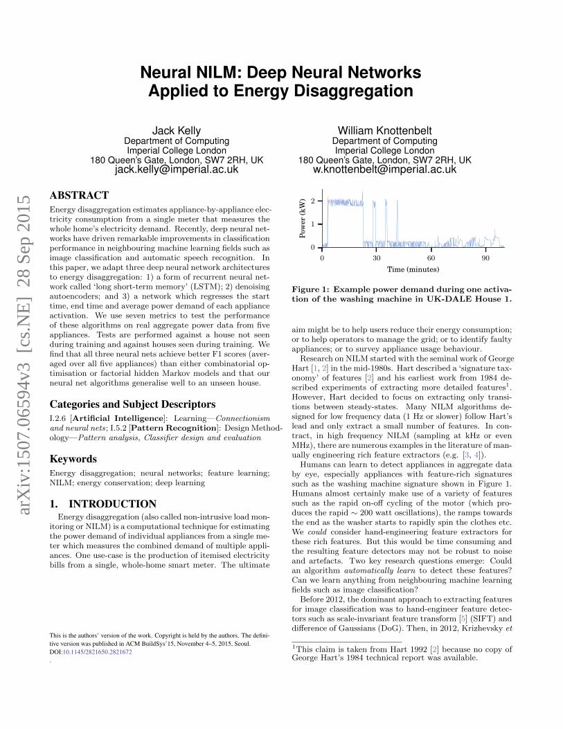
Figure 1: Example power demand during one activa-tion of the washing machine in UK-DALE House 1.

aim might be to help users reduce their energy consumption;or to help operators to manage the grid; or to identify faultyappliances; or to survey appliance usage behaviour.

Research on NILM started with the seminal work of GeorgeHart [1, 2] in the mid-1980s. Hart described a ‘signature tax-onomy’ of features [2] and his earliest work from 1984 de-scribed experiments of extracting more detailed features1.However, Hart decided to focus on extracting only transi-tions between steady-states. Many NILM algorithms de-signed for low frequency data (1 Hz or slower) follow Hart’slead and only extract a small number of features. In con-tract, in high frequency NILM (sampling at kHz or evenMHz), there are numerous examples in the literature of man-ually engineering rich feature extractors (e.g. [3, 4]).

Humans can learn to detect appliances in aggregate databy eye, especially appliances with feature-rich signaturessuch as the washing machine signature shown in Figure 1.Humans almost certainly make use of a variety of featuressuch as the rapid on-off cycling of the motor (which pro-duces the rapid ∼ 200 watt oscillations), the ramps towardsthe end as the washer starts to rapidly spin the clothes etc.We could consider hand-engineering feature extractors forthese rich features. But this would be time consuming andthe resulting feature detectors may not be robust to noiseand artefacts. Two key research questions emerge: Couldan algorithm automatically learn to detect these features?Can we learn anything from neighbouring machine learningfields such as image classification?

Before 2012, the dominant approach to extracting featuresfor image classification was to hand-engineer feature detec-tors such as scale-invariant feature transform [5] (SIFT) anddifference of Gaussians (DoG). Then, in 2012, Krizhevsky et

1This claim is taken from Hart 1992 [2] because no copy ofGeorge Hart’s 1984 technical report was available.

arX

iv:1

507.

0659

4v3

[cs

.NE

] 2

8 Se

p 20

15

al.’s winning algorithm [6] in the ImageNet Large Scale Vi-sual Recognition Challenge achieved a substantially lowererror score (15%) than the second-best approach (26%).Krizhevsky et al.’s approach did not use hand-engineeredfeature detectors. Instead they used a deep neural networkwhich automatically learnt to extract a hierarchy of featuresfrom the raw image. Deep learning is now a dominant ap-proach not only in image classification but also fields suchas automatic speech recognition [7], machine translation [8],even learning to play computer games from scratch [9]!

In this paper, we investigate whether deep neural nets canbe applied to energy disaggregation. The use of ‘small’ neu-ral nets on NILM dates back at least to Roos et al. 1994 [10](although that paper was just a proposal) and continuedwith [11, 12, 13, 14] but these small nets do not appear tolearn a hierarchy of feature detectors. A big breakthrough inimage classification came when the compute power (courtesyof GPUs) became available to train deep neural networks onlarge amounts of data. In the present research, we wantto see if deep neural nets can deliver good performance onenergy disaggregation.

Our main contribution is to adapt three deep neural net-work architectures to NILM. For each architecture, we trainone network per target appliance. We compare two bench-mark disaggregation algorithms (combinatorial optimisationand factorial hidden Markov models) to the disaggregationperformance of our three deep neural nets using seven met-rics. We also examine how well our neural nets generaliseto appliances in houses not seen during training because,ultimately, when NILM is used ‘in the field’ we very rarelyhave ground truth appliance data for the houses for whichwe want to disaggregate. So it is essential that NILM algo-rithms can generalise to unseen houses.

Please note that, once trained, our neural nets do not needground truth appliance data from each house! End-userswould only need to provide aggregate data. This is becauseeach neural network should learn the ‘essence’ of its targetappliance such that it can generalise to unseen instances ofthat appliance. In a similar fashion, neural networks trainedto do image classification are trained on many examples ofeach category (dogs, cats, etc.) and generalise to unseenexamples of each category.

To provide more context, we will briefly sketch how ourneural networks could be deployed at scale, in the wild. Eachnet would undergo supervised training on many examples ofits target appliance type so each network learns to generalisewell to unseen appliances.

Training is computationally expensive (days of processingon a fast GPU). But training does not have to be performedoften. Once these networks are trained, inference is muchcheaper (around a second of processing per network on a fastGPU for a week of aggregate data). Aggregate data fromunseen houses would be fed through each network. Eachnetwork should filter out the power demand for its targetappliance. This processing would probably be too computa-tionally expensive to run on an embedded processor insidea smart meter or in-home-display. Instead, the aggregatedata could be sent from the smart meter to the cloud. Thestorage requirements for one 16 bit integer sample (0-64 kWin 1 watt steps) every ten seconds is 17 kilobytes per dayuncompressed. This signal should be easily compressiblebecause there are numerous periods in domestic aggregatepower demand with little or no change. With a compres-

sion ratio of 5:1, and ignoring the datetime index, the totalstorage requirements for a year of data from 10 million userswould be 13 terabytes (which could fit on two 8 TB disks). Ifone week of aggregate data can be processed in one secondper home (which should be possible given further optimi-sation) then data from 10 million users could be processedby 16 GPU compute nodes. Alternatively, disaggregationcould be performed on a compute device within each home(a modern laptop or mobile phone or a dedicated ‘disaggre-gation hub’ could handle the disaggregation). A GPU is notrequired for disaggregation, although it makes it faster.

This paper is structured as follows: In Section 2 we pro-vide a very brief introduction to artificial neural nets. InSection 3 we describe how we prepare the training data forour nets and how we ‘augment’ the training data by syn-thesising additional data. In Section 4 we describe how weadapted three neural net architectures to NILM. In Section 5we describe how we do disaggregation with our nets. In Sec-tion 6 we present the disaggregation results of our threeneural nets and two benchmark NILM algorithms. Finally,in Section 7 discuss our results, offer our conclusions anddescribe some possible future directions for research.

2. INTRODUCTION TO NEURAL NETSAn artificial neural network (ANN) is a directed graph

where the nodes are artificial neurons and the edges allowinformation from one neuron to pass to another neuron (orthe same neuron in a future time step). Neurons are typ-ically arranged into layers such that each neuron in layerl connects to every neuron in layer l + 1. Connections areweighted and it is through modification of these weights thatANNs learn. ANNs have an input layer and an output layer.Any layers in between are called hidden layers. The forwardpass of an ANN is where information flows from the inputlayer, through any hidden layers, to the output. Learning(updating the weights) happens during the backwards pass.

2.1 Forwards passEach artificial neuron calculates a weighted sum of its in-

puts, adds a learnt bias and passes this sum through anactivation function. Consider a neuron which receives I in-puts. The value of each input is represented by input vectorx. The weight on the connection from input i to neuronh is denoted by wih (so w is the ‘weights matrix’). Theweighted sum (also called the ‘network input’) of the inputs

into neuron h can be written ah =∑I

i=1 xiwih. The net-work input ah is then passed through an activation functionθ to produce the neuron’s final output bh where bh = θ(ah).In this paper, we use the following activation functions: lin-ear: θ(x) = x; rectified linear (ReLU): θ(x) = max(0, x);

hyperbolic tangent (tanh): θ(x) = sinh xcosh x

= ex−e−x

ex+e−x .Multiple nonlinear hidden layers can be used to re-represent

the input data (hopefully by learning a hierarchy of featuredetectors), which gives deep nonlinear networks a great dealof expressive power [15, 16].

2.2 Backwards passThe basic idea of the backwards pass it to first do a for-

wards pass through the entire network to get the network’soutput for a specific network input. Then compute the errorof the output relative to the target (in all our experimentswe use the mean squared error (MSE) as the objective func-

tion). Then modify the weights in the direction which shouldreduce the error.

In practice, the forward pass is often computed over abatch of randomly selected input vectors. In our work, weuse a batch size of 64 sequences per batch for all but thelargest recurrent neural network (RNN) experiments. In ourlargest RNNs we use a batch size of 16 (to allow the networkto fit into the 3GB of RAM on our GPU).

How do we modify each weight to reduce the error? Itwould be computationally intractable to enumerate the en-tire error surface. MSE gives a smooth error surface andthe activation functions are differentiable hence we can usegradient descent. The first step is to compute the gradi-ent of the error surface at the position for current batch bycalculating the derivative of the objective function with re-spect to each weight. Then we modify each weight by addingthe gradient multiplied by a ‘learning rate’ scalar parame-ter. To efficiently compute the gradient (in O(W ) time) weuse the backpropagation algorithm [17, 18, 19]. In all ourexperiments we use stochastic gradient descent (SGD) withNesterov momentum of 0.9.

2.3 Convolutional neural netsConsider the task of identifying objects in a photograph.

No matter if we hand engineer feature detectors or learn fea-ture detectors from the data, it turns out that useful ‘lowlevel’ features concern small patches of the image and in-clude features such as edges of different orientations, cor-ners, blobs etc. To extract these features, we want to builda small number of feature detectors (one for horizontal lines,one for blobs etc.) with small receptive fields (overlappingsub-regions of the input image) and slide these feature de-tectors across the entire image. Convolutional neural nets(CNNs) [20, 21, 22] build a small number of filters, eachwith a small receptive field, and these filters are duplicated(with shared weights) across the entire input.

Similarly to computer vision tasks, in time series problemswe often want to extract a small number of low level featureswith a small receptive fields across the entire input. All ofour nets use at least one 1D convolutional layer at the input.

3. TRAINING DATADeep neural nets need a lot of training data because they

have a large number of trainable parameters (the networkweights and biases). The nets described in this paper havebetween 1 million to 150 million trainable parameters. Largetraining datasets are important. It is also common practicein deep learning to increase the effective size of the trainingset by duplicating the training data many times and apply-ing realistic transformations to each copy. For example, inimage classification, we might flip the image horizontally orapply slight affine transformations.

A related approach to creating a large training dataset isto generate simulated data. For example, Google DeepMindtrain their algorithms [9] on computer games because theycan generate an effectively infinite amount of training data.Realistic synthetic speech audio data or natural images areharder to produce.

In energy disaggregation, we have the advantage that gen-erating effectively infinite amounts of synthetic aggregatedata is relatively easy by randomly combining real appli-ance activations. (We define an ‘appliance activation’ to bethe power drawn by a single appliance over one complete cy-

cle of that appliance. For example, Figure 1 shows a singleactivation for a washing machine.) We trained our nets onboth synthetic aggregate data and real aggregate data in a50:50 ratio. We found that synthetic data acts as a regu-lariser. In other words, training on a mix of synthetic andreal aggregate data rather than just real data appears toimprove the net’s ability to generalise to unseen houses. Forvalidation and testing we use only real data (not synthetic).

We used UK-DALE [23] as our source dataset. Eachsubmeter in UK-DALE samples once every 6 seconds. Allhouses record aggregate apparent mains power once every6 seconds. Houses 1, 2 and 5 also record active and reactivemains power once a second. In these houses, we downsam-pled the 1 second active mains power to 6 seconds to alignwith the submetered data and used this as the real aggre-gate data from these houses. Any gaps in appliance datashorter than 3 minutes are assumed to be due to RF issuesand so are filled by forward-filling. Any gaps longer than3 minutes are assumed to be due to the appliance and meterbeing switched off and so are filled with zeros.

We manually checked a random selection of appliance ac-tivations from every house. The UK-DALE metadata showsthat House 4’s microwave and washing machine share a sin-gle meter (a fact that we manually verified) and hence theseappliances from House 4 are not used in our training data.

We train one network per target appliance. The target(i.e. the desired output of the net) is the power demand ofthe target appliance. The input to every net we describein this paper is a window of aggregate power demand. Thewindow width is decided on an appliance-by-appliance basisand varies from 128 samples (13 minutes) for the kettle to1536 samples (2.5 hours) for the dish washer. We found thatincreasing the window size hurts disaggregation performancefor short-duration appliances (for example, using a sequencelength of 1024 for the fridge resulted in the autoencoder(AE) failing to learn anything useful and the ‘rectangles’ netachieved an F1 score of 0.68; reducing the sequence lengthto 512 allowed the AE to get an F1 score of 0.87 and the‘rectangles’ net got a score of 0.82). On the other hand, it isimportant to ensure that the window width is long enoughto capture the majority of the appliance activations.

For each house, we reserved the last week of data for test-ing and used the rest of the data for training. The numberof appliance training activations is show in Table 1 and thenumber of testing activations is shown in Table 2. The spe-cific houses used for training and testing is shown in Table 3.

3.1 Choice of appliancesWe used five target appliances in all our experiments: the

fridge, washing machine, dish washer, kettle and microwave.We chose these appliances because each is present in at leastthree houses in UK-DALE. This means that, for each appli-ance, we can train our nets on at least two houses and teston a different house. These five appliances consume a signif-icant proportion of energy and the five appliances representa range of different power ‘signatures’ from the simple on/offof the kettle to the complex pattern shown by the washingmachine (Figure 1).

‘Small’ appliances such as games consoles and phone charg-ers are problematic for many NILM algorithms because theeffect of small appliances on aggregate power demand tendsto get lost in the noise. By definition, small appliances donot consume much energy individually but modern homes

tend to have a large number of such appliances so their com-bined consumption can be significant. Hence it would beuseful to detect small appliances using NILM. We have notexplored whether our neural nets perform well on ‘small’appliances but we plan to in the future.

3.2 Extract activationsAppliance activations are extracted using NILMTK’s [24]

Electric.get_activations() method. The arguments wepassed to get_activations() for each appliance are shownin Table 4. On simple appliances such as toasters, we extractactivations by finding strictly consecutive samples above somethreshold power. We then throw away any activations shorterthan some threshold duration (to ignore spurious spikes).For more complex appliances such as washing machines whosepower demand can drop below threshold for short periodsduring a cycle, NILMTK ignores short periods of sub-thresholdpower demand.

3.3 Select windows of real aggregate dataFirst we locate all the activations of the target appliance

in the home’s submeter data for the target appliance. Then,for each training example, the code decides with 50% prob-ability whether this example should include the target ap-pliance or not. If the code decides not include the targetappliance then it finds a random window of aggregate datain which there are no activations of the target appliance.Otherwise, the code randomly selects a target appliance ac-tivation and randomly positions this activation within thewindow of data that will be shown to the net as the target(with the constraint that the activation must be capturedcompletely in the window of data shown to the net, unlessthe window is too short to contain the entire activation).The corresponding time window of real aggregate data isalso loaded and shown to the net and its input. If otheractivations of the target appliance happen to appear in theaggregate data then these are not included in the targetsequence; the net is trained to focus on the first completetarget appliance activation in the aggregate data.

3.4 Synthetic aggregate dataTo create synthetic aggregate data we start by extract-

ing a set of appliance activations for five appliances acrossall training houses: kettle, washing machine, dish washer,microwave and fridge. To create a single sequence of syn-thetic data, we start with two vectors of zeros: one vectorwill become the input to the net; the other will become thetarget. The length of each vector defines the ‘window width’of data that the network sees. We go through the five appli-ance classes and decide whether or not to add an activationof that class to the training sequence. There is a 50% chancethat the target appliance will appear in the sequence and a25% chance for each other ‘distractor’ appliance. For eachselected appliance class, we randomly select an applianceactivation and then randomly pick where to add that acti-vation on the input vector. Distractor appliances can appearanywhere in the sequence (even if this means that only partof the activation will be included in the sequence). Thetarget appliance activation must be completely containedwithin the sequence (unless it is too large to fit).

Of course, this relatively naıve approach to synthesisingaggregate data ignores a lot of structure that appears inreal aggregate data. For example, the kettle and toaster

Table 1: Number of training activations per house.

1 2 3 4 5

Kettle 2836 543 44 716 176Fridge 16 336 3526 0 4681 1488Washing machine 530 53 0 0 51Microwave 3266 387 0 0 28Dish washer 197 98 0 23 0

Table 2: Number of testing activations per house.

1 2 3 4 5

Kettle 54 29 40 50 18Fridge 168 277 0 145 140Washing machine 10 4 0 0 2Microwave 90 9 0 0 4Dish washer 3 7 0 3

might often appear within a few minutes of each other inreal data, but our simple ‘simulator’ is completely unawareof this sort of structure. We expect that a more realisticsimulator might increase the performance of deep neural netson energy disaggregation.

3.5 Implementation of data processingAll our code is written in Python and we make use Pandas,

Numpy and NILMTK for data preparation. Each networkreceives data in a mini-batch of 64 sequences (except for thelarge RNN sequences, in which case we use a batch size of16 sequences). The code is multi-threaded so the CPU canbe busy preparing one batch of data on the fly whilst theGPU is busy training on the previous batch.

3.6 StandardisationIn general, neural nets learn most efficiently if the input

data has zero mean. First, the mean of each sequence issubtracted from the sequence to give each sequence a meanof zero. Every input sequence is divided by the standarddeviation of a random sample of the training set. We do notdivide each sequence by its own standard deviation becausethat would change the scaling and the scaling is likely to beimportant for NILM.

Forcing each sequence to have zero mean throws away in-formation. Information that NILM algorithms such as com-binatorial optimisation and factorial hidden Markov modelsrely on. We have done some preliminary experiments andfound that neural nets appear to be able to generalise bet-ter if we independently centre each sequence. But thereare likely to be ways to have the best of both worlds: i.e.to give the network information about the absolute powerwhilst also allowing the network to generalise well.

One big advantage of training our nets on sequences whichhave been independently centred is that our nets do not needto consider vampire (always on) loads.

Targets are divided by a hand-coded ‘maximum powerdemand’ for each appliance to put the target power demandinto the range [0, 1].

4. NEURAL NETWORK ARCHITECTURESIn this section we describe how we adapted three different

neural net architectures to do NILM.

Table 3: Houses used for training and testing.

Training Testing

Kettle 1, 2, 3, 4 5Fridge 1, 2, 4 5Washing machine 1, 5 2Microwave 1, 2 5Dish washer 1, 2 5

Table 4: Arguments passed to get_activations().

Max On power Min. on Min. offAppliance power threshold duration duration

(watts) (watts) (secs) (secs)

Kettle 3100 2000 12 0Fridge 300 50 60 12Washing m. 2500 20 1800 160Microwave 3000 200 12 30Dish washer 2500 10 1800 1800

4.1 Recurrent Neural NetworksIn Section 2 we described feed forward neural networks

which map from a single input vector to a single outputvector. When the network is shown a second input vector,it has no memory of the previous input.

Recurrent neural networks (RNNs) allow cycles in the net-work graph such that the output from neuron i in layer l attime step t is fed via weighted connections to every neuronin layer l (including neuron i) at time step t+1. This allowsRNNs, in principal, to map from the entire history of theinputs to an output vector. This makes RNNs especiallywell suited to sequential data. In our work, we train RNNsusing backpropagation through time (BPTT) [25].

In practice, RNNs can suffer from the ‘vanishing gradient’problem [26] where gradient information disappears or ex-plodes as it is propagated back through time. This can limitan RNN’s memory. One solution to this problem is the ‘longshort-term memory’ (LSTM) architecture [26] which uses a‘memory cell’ with a gated input, gated output and gatedfeedback loop. The intuition behind LSTM is that it is adifferentiable latch (where a ‘latch’ is the fundamental unitof a digital computer’s RAM). LSTMs have been used withsuccess on a wide variety of sequence tasks including auto-matic speech recognition [7, 27] and machine translation [8].

An additional enhancement to RNNs is to use bidirectionallayers. In a bidirectional RNN, there are effectively two par-allel RNNs, one reads the input sequence forwards and theother reads the input sequence backwards. The output fromthe forwards and backwards halves of the network are com-bined either by concatenating them or doing an element-wisesum (we experimented with both and settled on concatena-tion, although element-wise sum appeared to work almostas well and is computationally cheaper).

We should note that bidirectional RNNs are not naturallysuited to doing online disaggregation. Bidirectional RNNscould still be used for online disaggregation if we frame ‘on-line disaggregation’ as doing frequent, small batches of offlinedisaggregation.

We experimented with both RNNs and LSTMs and settledon the following architecture for energy disaggregation:

1. Input (length determined by appliance duration)

2. 1D conv (filter size=4, stride=1, number of filters=16,activation function=linear, border mode=same)

3. bidirectional LSTM (N=128, with peepholes)

4. bidirectional LSTM (N=256, with peepholes)

5. Fully connected (N=128, activation function=TanH)

6. Fully connected (N=1, activation function=linear)

At each time step, the network sees a single sample ofaggregate power data and outputs a single sample of powerdata for the target appliance.

In principal, the convolutional layer should not be neces-sary (because the LSTMs should be able to remember all thecontext). But we found the addition of a convolution layerto slightly increase performance (the conv. layer convolvesover the time axis). We also experimented with adding aconv. layer between the two LSTM layers with a stride > 1to implement hierarchical subsampling [28]. This showedpromise but we did not use it for our final experiments.

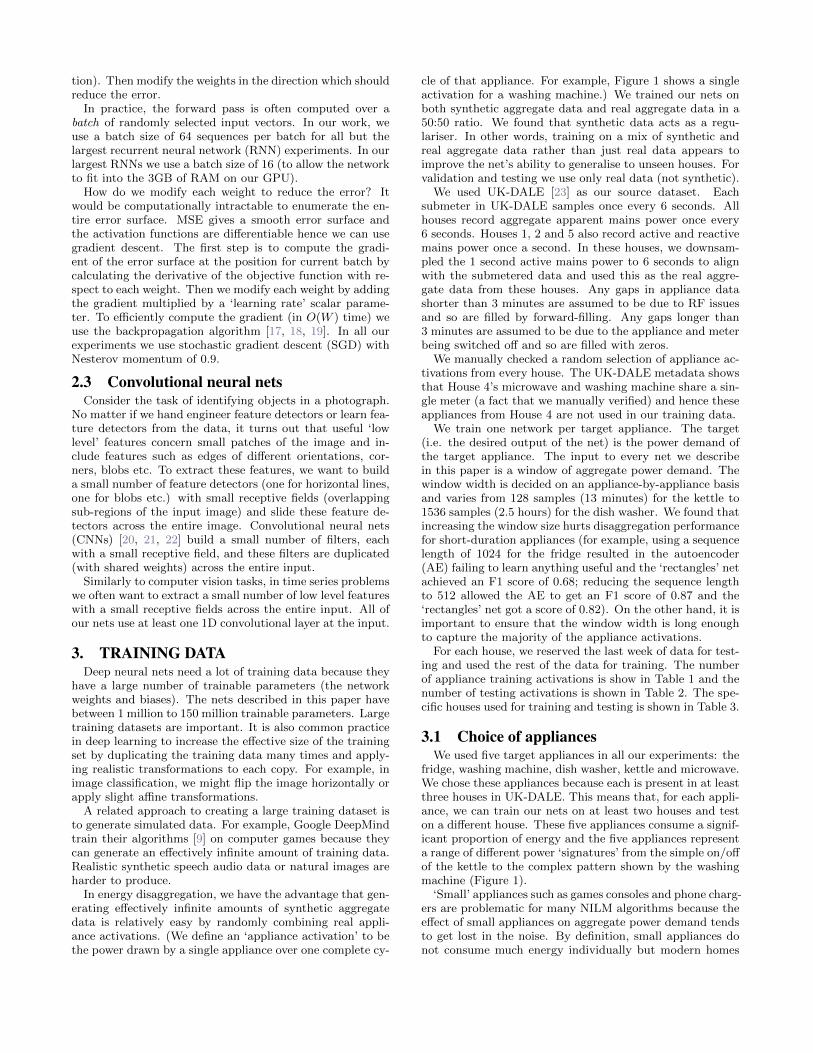
On the backwards pass, we clip the gradient at [-10, 10] asper Alex Graves in [29]. To speed up computation, we prop-agate the gradient backwards a maximum of 500 time steps.Figure 2 shows an example output of our LSTM network inthe two ‘RNN’ rows.

4.2 Denoising AutoencodersIn this section, we frame energy disaggregation as a ‘de-

noising’ task. Typical denoising tasks include removing grainfrom an old photograph; or removing reverb from an audiorecording; or even in-filling a masked part of an image. En-ergy disaggregation can be viewed as an attempt to recoverthe ‘clean’ power demand signal of the target appliance fromthe background ‘noise’ produced by the other appliances. Asuccessful neural network architecture for denoising tasks isthe ‘denoising autoencoder’.

An autoencoder (AE) is simply a network which tries toreconstruct the input. Described like this, AEs might notsound very useful! The key is that AEs first encode the in-put to a compact vector representation (in the ‘code layer’)and then decode to reconstruct the input. The simplest wayof forcing the net to discover a compact representation of thedata is to have a code layer with less dimensions than theinput. In this case, the AE is doing dimensionality reduc-tion. Indeed, a linear AE with a single hidden layer is almostequivalent to PCA. But AEs can be deep and non-linear.

A denoising autoencoder (dAE) [30] is an autoencoderwhich attempts to reconstruct a clean target from a noisyinput. dAEs are typically trained by artificially corruptinga signal before it goes into the net’s input, and using theclean signal as the net’s target. In NILM, we consider thecorruption as being the power demand from the other ap-pliances. So we do not add noise artificially. Instead we usethe aggregate power demand as the (noisy) input to the netand ask the net to reconstruct the clean power demand ofthe target appliance.

The first and last layers of our NILM dAEs are 1D con-volutional layers. We use convolutional layers because wewant the network to learn low level feature detectors whichare applied equally across the entire input window (for ex-ample, a step change of 1000 watts might be a useful featureto extract, no matter where it is found in the input). The

aim is to provide some invariance to where exactly the acti-vation is positioned within the input window. The last layerdoes a ‘deconvolution’.

The exact architecture is as follows:

1. Input (length determined by appliance duration)

2. 1D conv (filter size=4, stride=1, number of filters=8,activation function=linear, border mode=valid)

3. Fully connected (N=(sequence length - 3) × 8,activation function=ReLU)

4. Fully connected (N=128; activation function=ReLU)

5. Fully connected (N=(sequence length - 3) × 8,activation function=ReLU)

6. 1D conv (filter size=4, stride=1, number of filters=1,activation function=linear, border mode=valid)

Layer 4 is the middle, code layer. The entire dAE istrained end-to-end in one go (we do not do layer-wise pre-training as we found it did not increase performance). We donot tie the weights as we found this also appears to not en-hance NILM performance. An example output of our NILMdAE is shown in Figure 2 in the two ‘Autoencoder’ rows.

4.3 Regress Start Time, End Time & PowerMany applications of energy disaggregation do not require

a detailed second-by-second reconstruction of the appliancepower demand. Instead, most energy disaggregation use-cases require, for each appliance activation, the identificationof the start time, end time and energy consumed. In otherwords, we want to draw a rectangle around each applianceactivation in the aggregate data where the left side of therectangle is the start time, the right side is the end time andthe height is the average power demand of the appliancebetween the start and end times.

Deep neural networks have been used with great successon related tasks. For example, Nouri used deep neural net-works to estimate the 2D location of ‘facial keypoints’ inimages of faces [31]. Example ‘keypoints’ are ‘left eye cen-tre’ or ‘mouth centre top lip’. The input to Nouri’s neuralnet is the raw image of a face. The output of the network isa set of x, y coordinates for each keypoint.

Our idea was to train a neural network to estimate threescalar, real-valued outputs: the start time, the end timeand mean power demand of the first appliance activation toappear in the aggregate power signal. If there is no targetappliance in the aggregate data then all three outputs shouldbe zero. If there is more than one activation in the aggre-gate signal then the network should ignore all but the firstactivation. All outputs are in the range [0, 1]. The startand end times are encoded as a proportion of the input’stime window. For example, the start of the time window isencoded as 0, the end is encoded as 1 and half way throughthe time window is encoded as 0.5. For example, considera scenario where the input window width is 10 minutes andan appliance activation starts 1 minute into the window andends 1 minute before the end of the window. This activationwould be encoded as having a start location of 0.1 and anend location of 0.9. Example output is shown in Figure 2 inthe two ‘Rectangles’ rows.

The three target values for each sequence are calculatedduring data pre-processing. As for all of our other networks,the network’s objective is to minimise the mean squarederror. The exact architecture is as follows:

1. Input (length determined by appliance duration)

2. 1D conv (filter size=4, stride=1, number of filters=16,activation function=linear, border mode=valid)

3. 1D conv (filter size=4, stride=1, number of filters=16,activation function=linear, border mode=valid)

4. Fully connected (N=4096, activation function=ReLU)

5. Fully connected (N=3072; activation function=ReLU)

6. Fully connected (N=2048, activation function=ReLU)

7. Fully connected (N=512, activation function=ReLU)

8. Fully connected (N=3, activation function=linear)

4.4 Neural net implementationWe implemented our neural nets in Python using the

Lasagne library2. Lasagne is built on top of Theano [32,33]. We trained our nets on an nVidia GTX 780Ti GPUwith 3 GB of RAM (but note that Theano also allows codeto be run on the CPU without requiring any changes to theuser’s code). On this GPU, our nets typically took between1 and 12 hours to train per appliance. The exact code usedto create the results in paper is available in our ‘NeuralNILMPrototype’ repository3 and a more elegant (hopefully!) re-write is available in our ‘NeuralNILM’ repository4.

We manually defined the number of weight updates to per-form during training for each experiment. For the RNNs weperformed 10,000 updates, for the denoising autoencoderswe performed 100,000 and for the regression network weperformed 300,000 updates. Neither the RNNs nor the AEsappeared to continue learning past this number of updates.The regression networks appear to keep learning no matterhow many updates we perform!

The nets have a wide variation in the number of trainableparameters. The largest dAE nets range from 1M to 150M(depending on the input size); the RNNs all had 1M pa-rameters and the regression nets varied from 28M to 120Mparameters (depending on the input size).

All our network weights were initialised randomly usingLasagne’s default initialisation. All of the experiments pre-sented in this paper trained end-to-end from random initial-isation (no layerwise pre-training).

5. DISAGGREGATIONHow do we disaggregate arbitrarily long sequences of ag-

gregate data given that each net has an input window dura-tion of, at most, a few hours? We first pad the beginning andend of the input with zeros. Then we slide the net along theinput sequence. As such, the first sequence we show to thenetwork will be all zeros. Then we shift the input windowSTRIDE samples to the right, where STRIDE is a manuallydefined positive, non-zero integer. If STRIDE is less than thelength of the net’s input window then the net will see over-lapping input sequences. This allows the network to havemultiple attempts at processing each appliance activation inthe aggregate signal, and on each attempt each activationwill be shifted to the left by STRIDE samples.

Over the course of disaggregation, the network producesmultiple estimated values for each time step because we givethe network overlapping segments of the input. For our first

2github.com/Lasagne/Lasagne3github.com/JackKelly/neuralnilm prototype4github.com/JackKelly/neuralnilm

two network architectures, we combine the multiple valuesper timestep simply by taking the mean.

Combing the output from our third network is a little morecomplex. We layer every predicted ‘appliance rectangle’ ontop of each other. We measure the overlap and normalise theoverlap to [0, 1]. This gives a probabilistic output for eachappliance’s power demand. To convert this to a single vectorper appliance, we threshold the power and probability.

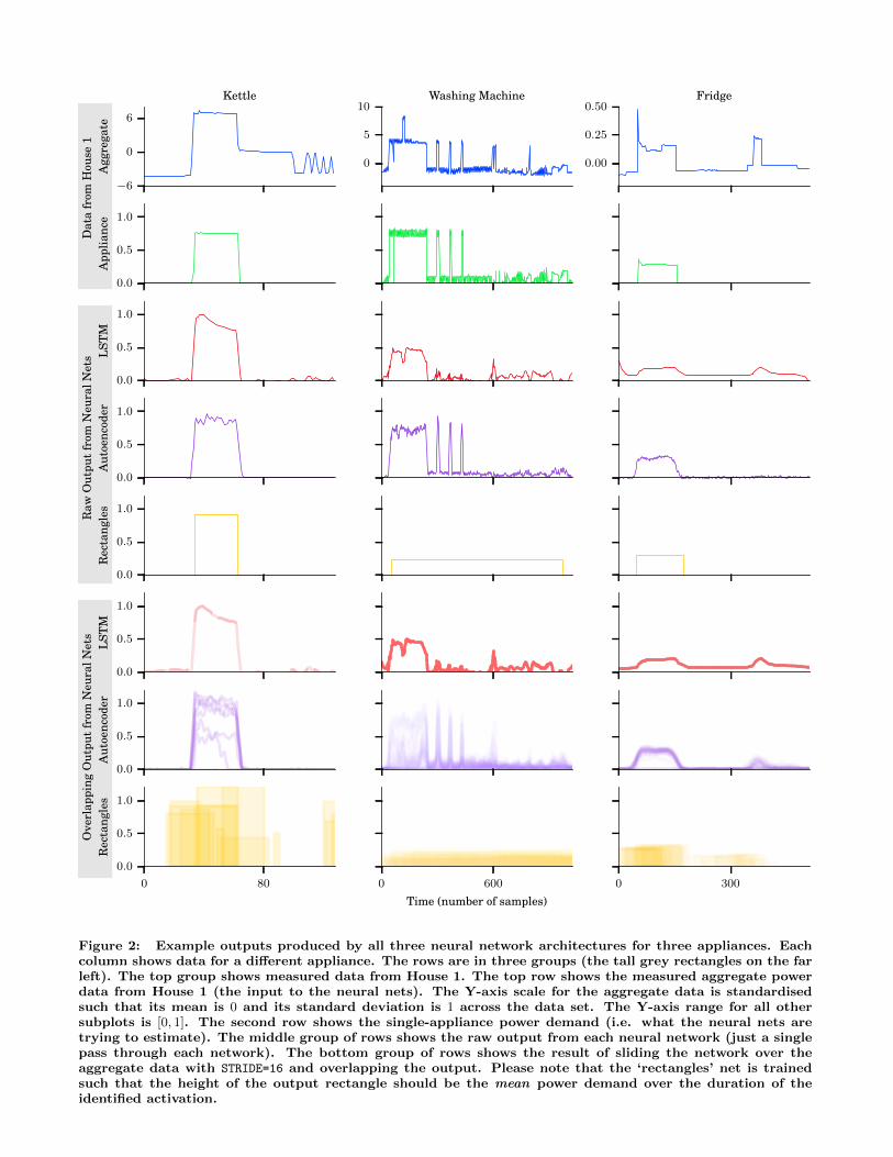
6. RESULTSThe disaggregation results on an unseen house are shown

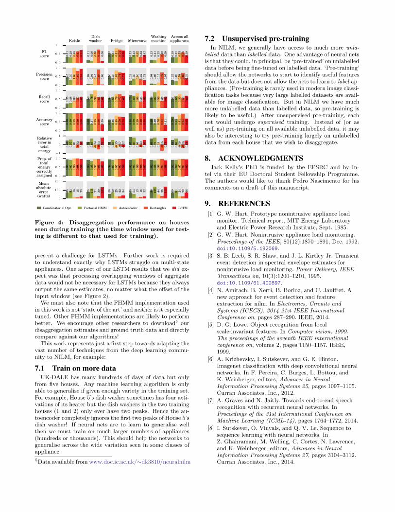
in Figure 3. The results on houses seen during training areshown in Figure 4.

We used benchmark implementations from NILMTK [24]of the combinatorial optimisation (CO) and factorial hiddenMarkov model (FHMM) algorithms.

On the unseen house (Figure 3), both the denoising au-toencoder and the net which regresses the start time, endtime and power demand (the ‘rectangles’ architecture) out-perform CO and FHMM on every appliance on F1 score,precision score, proportion of total energy correctly assignedand mean absolute error. The LSTM out-performs CO andFHMM on two-state appliances (kettle, fridge and microwave)but falls behind CO and FHMM on multi-state appliances(dish washer and washing machine).

On the houses seen during training (Figure 4), the dAEoutperforms CO and FHMM on every appliance on everymetric except relative error in total energy. The ‘rectangles’architecture outperforms CO and FHMM on every appliance(except the microwave) on F1, precision, accuracy, propor-tion of total energy correctly assigned and mean absoluteerror.

The full disaggregated time series for all our algorithmsand the aggregate data and appliance ground truth data areavailable at www.doc.ic.ac.uk/∼dk3810/neuralnilm

The metrics we used are:

TP = number of true positives (1)

FP = number of false positives (2)

FN = number of false negatives (3)

P = number of positives in ground truth (4)

N = number of negatives in ground truth (5)

E = total actual energy (6)

E = total predicted energy (7)

y(i)t = appliance i actual power at time t (8)

y(i)t = appliance i estimated power at time t (9)

yt = aggregate actual power at time t (10)

recall =TP

TP + FN(11)

precision =TP

TP + FP(12)

F1 = 2× precision× recall

precision + recall(13)

accuracy =TP + TN

P + N(14)

relative error in total energy =|E − E|

max(E, E)(15)

0.0

0.5

1.0

F1score 0.

310.

190.

930.

700.

93

Kettle

0.11

0.05

0.44

0.74

0.08

Dishwasher

0.35

0.55

0.87

0.82

0.74

Fridge

0.05

0.01

0.26

0.21

0.13

Microwave

0.10

0.08

0.13

0.27

0.03

Washingmachine

0.18

0.18

0.53

0.55

0.38

Across allappliances

0.0

0.5

1.0

Precisionscore 0.

230.

141.

000.

700.

96

0.06

0.03

0.29

0.89

0.04

0.30

0.40

0.85

0.79

0.72

0.03

0.01

0.15

0.14

0.07

0.06

0.04

0.07

0.29

0.01

0.13

0.12

0.47

0.56

0.36

0.0

0.5

1.0

Recallscore 0.

460.

290.

870.

710.

91

0.67

0.49

0.99

0.64

0.87

0.41

0.86

0.88

0.86

0.77

0.35

0.34

0.94

0.40

0.99

0.48

0.64

1.00

0.24

0.73

0.47

0.53

0.94

0.57

0.85

0.0

0.5

1.0

Accuracyscore 0.

990.

991.

001.

001.

00

0.64

0.33

0.92

0.99

0.30

0.45

0.50

0.90

0.87

0.81

0.98

0.91

0.99

0.99

0.98

0.88

0.79

0.82

0.98

0.23

0.79

0.70

0.93

0.97

0.66

−1

0

1Relativeerror in

totalenergy

0.85

0.88

0.13

0.03

0.57

0.62

0.75

-0.3

3-0

.31

0.87

0.37

0.57

-0.3

8-0

.13

-0.2

5

0.97

0.99

0.73

0.50

0.88

0.73

0.86

0.48

-0.7

40.

91

0.71

0.81

0.12

-0.1

30.

59

0.0

0.5

1.0Prop. oftotal

energycorrectlyassigned

0.94

0.92

1.00

0.99

0.99

0.94

0.91

0.98

0.98

0.86

0.94

0.94

0.98

0.99

0.97

0.93

0.84

0.99

1.00

0.98

0.93

0.88

0.96

0.98

0.81

0.94

0.90

0.98

0.99

0.92

0

100

200Mean

absoluteerror

(watts)

73 98 6 7 16 74 110

24 30 168

73 67 26 18 36 89 195 9 6 20 39 67 24 11 109

70 107

18 14 70

Combinatorial Opt. Factorial HMM Autoencoder Rectangles LSTM

Figure 3: Disaggregation performance on a housenot seen during training.

mean absolute error = 1/T

T∑t=1

|yt − yt| (16)

proportion of total energy correctly assigned =

1−∑T

t=1

∑ni=1 |y

(i)t − y

(i)t |

2∑T

t=1 yt(17)

The proportion of total energy correctly assigned is takenfrom [34].

7. CONCLUSIONS & FUTURE WORKWe have adapted three neural network architectures to

NILM. The denoising autoencoder and the ‘rectangles’ ar-chitectures perform well, especially on unseen houses. Webelieve that deep neural nets show great promise for NILM.But there is plenty of work still to do!

It is worth noting that our comparison between each ar-chitecture is not entirely fair because the architectures havea wide range of trainable parameters. For example, everyLSTM we used had 1M parameters whilst the larger dAEand rectangles nets had over 150M parameters (we did trytraining an LSTM with more parameters but it did not ap-pear to improve performance).

Our LSTM results suggest that LSTMs work best for two-state appliances but do not perform well on multi-state ap-pliances such as the dish washer and washing machine. Onepossible reason is that, for these appliances, informative‘events’ in the power signal can be many time steps apart(e.g. for the washing machine there might be over 1,000time steps between the first heater activation and the spincycle). In principal, LSTMs have an arbitrarily long mem-ory. But these long gaps between informative events may

−6

0

6A

ggre

gate

Kettle

0

5

10Washing Machine

0.00

0.25

0.50Fridge

0.0

0.5

1.0

App

lianc

e

0.0

0.5

1.0

LST

M

0.0

0.5

1.0

Aut

oenc

oder

0.0

0.5

1.0

Rec

tang

les

0.0

0.5

1.0

LST

M

0.0

0.5

1.0

Aut

oenc

oder

0 80

0.0

0.5

1.0

Rec

tang

les

0 600

Time (number of samples)0 300

Dat

afr

omH

ouse

1R

awO

utpu

tfr

omN

eura

lNet

sO

verl

appi

ngO

utpu

tfr

omN

eura

lNet

s

Figure 2: Example outputs produced by all three neural network architectures for three appliances. Eachcolumn shows data for a different appliance. The rows are in three groups (the tall grey rectangles on the farleft). The top group shows measured data from House 1. The top row shows the measured aggregate powerdata from House 1 (the input to the neural nets). The Y-axis scale for the aggregate data is standardisedsuch that its mean is 0 and its standard deviation is 1 across the data set. The Y-axis range for all othersubplots is [0, 1]. The second row shows the single-appliance power demand (i.e. what the neural nets aretrying to estimate). The middle group of rows shows the raw output from each neural network (just a singlepass through each network). The bottom group of rows shows the result of sliding the network over theaggregate data with STRIDE=16 and overlapping the output. Please note that the ‘rectangles’ net is trainedsuch that the height of the output rectangle should be the mean power demand over the duration of theidentified activation.

0.0

0.5

1.0

F1score 0.

310.

280.

480.

630.

71

Kettle

0.11

0.08

0.60

0.72

0.06

Dishwasher

0.52

0.47

0.81

0.74

0.69

Fridge

0.33

0.43

0.62

0.32

0.42

Microwave

0.13

0.11

0.25

0.49

0.09

Washingmachine

0.28

0.27

0.55

0.58

0.39

Across allappliances

0.0

0.5

1.0

Precisionscore 0.

450.

301.

000.

800.

91

0.07

0.04

0.45

0.88

0.03

0.50

0.39

0.83

0.71

0.71

0.24

0.35

0.50

0.32

0.28

0.08

0.06

0.15

0.72

0.05

0.27

0.23

0.58

0.69

0.39

0.0

0.5

1.0

Recallscore 0.

250.

280.

390.

570.

63

0.50

0.78

0.99

0.61

0.63

0.54

0.63

0.79

0.77

0.67

0.70

0.69

0.86

0.34

0.92

0.56

0.87

0.99

0.38

0.62

0.51

0.65

0.80

0.53

0.69

0.0

0.5

1.0

Accuracyscore 0.

990.

990.

990.

991.

00

0.69

0.37

0.95

0.98

0.35

0.61

0.46

0.85

0.79

0.76

0.98

0.99

0.99

0.99

0.98

0.69

0.39

0.76

0.97

0.31

0.79

0.64

0.91

0.94

0.68

−1

0

1Relativeerror in

totalenergy

0.43

0.57

0.02

-0.3

20.

36

0.28

0.66

-0.3

4-0

.53

0.76

0.26

0.50

-0.3

5-0

.07

-0.2

2

0.85

0.80

0.06

-0.2

30.

50

0.65

0.76

0.18

-0.6

50.

73

0.49

0.66

-0.0

9-0

.36

0.43

0.0

0.5

1.0Prop. oftotal

energycorrectlyassigned

0.93

0.91

0.98

0.98

0.98

0.90

0.85

0.97

0.96

0.83

0.94

0.91

0.97

0.97

0.96

0.92

0.93

0.99

0.98

0.97

0.92

0.88

0.96

0.97

0.88

0.92

0.90

0.97

0.97

0.92

0

100

200Mean

absoluteerror

(watts)

65 82 16 15 23 75 111

21 30 130

50 69 25 22 34 68 54 13 16 22 88 138

44 28 133

69 91 24 22 68

Combinatorial Opt. Factorial HMM Autoencoder Rectangles LSTM

Figure 4: Disaggregation performance on housesseen during training (the time window used for test-ing is different to that used for training).

present a challenge for LSTMs. Further work is requiredto understand exactly why LSTMs struggle on multi-stateappliances. One aspect of our LSTM results that we did ex-pect was that processing overlapping windows of aggregatedata would not be necessary for LSTMs because they alwaysoutput the same estimates, no matter what the offset of theinput window (see Figure 2).

We must also note that the FHMM implementation usedin this work is not ‘state of the art’ and neither is it especiallytuned. Other FHMM implementations are likely to performbetter. We encourage other researchers to download5 ourdisaggregation estimates and ground truth data and directlycompare against our algorithms!

This work represents just a first step towards adapting thevast number of techniques from the deep learning commu-nity to NILM, for example:

7.1 Train on more dataUK-DALE has many hundreds of days of data but only

from five houses. Any machine learning algorithm is onlyable to generalise if given enough variety in the training set.For example, House 5’s dish washer sometimes has four acti-vations of its heater but the dish washers in the two traininghouses (1 and 2) only ever have two peaks. Hence the au-toencoder completely ignores the first two peaks of House 5’sdish washer! If neural nets are to learn to generalise wellthen we must train on much larger numbers of appliances(hundreds or thousands). This should help the networks togeneralise across the wide variation seen in some classes ofappliance.

5Data available from www.doc.ic.ac.uk/∼dk3810/neuralnilm

7.2 Unsupervised pre-trainingIn NILM, we generally have access to much more unla-

belled data than labelled data. One advantage of neural netsis that they could, in principal, be ‘pre-trained’ on unlabelleddata before being fine-tuned on labelled data. ‘Pre-training’should allow the networks to start to identify useful featuresfrom the data but does not allow the nets to learn to label ap-pliances. (Pre-training is rarely used in modern image classi-fication tasks because very large labelled datasets are avail-able for image classification. But in NILM we have muchmore unlabelled data than labelled data, so pre-training islikely to be useful.) After unsupervised pre-training, eachnet would undergo supervised training. Instead of (or aswell as) pre-training on all available unlabelled data, it mayalso be interesting to try pre-training largely on unlabelleddata from each house that we wish to disaggregate.

8. ACKNOWLEDGMENTSJack Kelly’s PhD is funded by the EPSRC and by In-

tel via their EU Doctoral Student Fellowship Programme.The authors would like to thank Pedro Nascimento for hiscomments on a draft of this manuscript.

9. REFERENCES[1] G. W. Hart. Prototype nonintrusive appliance load

monitor. Technical report, MIT Energy Laboratoryand Electric Power Research Institute, Sept. 1985.

[2] G. W. Hart. Nonintrusive appliance load monitoring.Proceedings of the IEEE, 80(12):1870–1891, Dec. 1992.doi:10.1109/5.192069.

[3] S. B. Leeb, S. R. Shaw, and J. L. Kirtley Jr. Transientevent detection in spectral envelope estimates fornonintrusive load monitoring. Power Delivery, IEEETransactions on, 10(3):1200–1210, 1995.doi:10.1109/61.400897.

[4] N. Amirach, B. Xerri, B. Borloz, and C. Jauffret. Anew approach for event detection and featureextraction for nilm. In Electronics, Circuits andSystems (ICECS), 2014 21st IEEE InternationalConference on, pages 287–290. IEEE, 2014.

[5] D. G. Lowe. Object recognition from localscale-invariant features. In Computer vision, 1999.The proceedings of the seventh IEEE internationalconference on, volume 2, pages 1150–1157. IEEE,1999.

[6] A. Krizhevsky, I. Sutskever, and G. E. Hinton.Imagenet classification with deep convolutional neuralnetworks. In F. Pereira, C. Burges, L. Bottou, andK. Weinberger, editors, Advances in NeuralInformation Processing Systems 25, pages 1097–1105.Curran Associates, Inc., 2012.

[7] A. Graves and N. Jaitly. Towards end-to-end speechrecognition with recurrent neural networks. InProceedings of the 31st International Conference onMachine Learning (ICML-14), pages 1764–1772, 2014.

[8] I. Sutskever, O. Vinyals, and Q. V. Le. Sequence tosequence learning with neural networks. InZ. Ghahramani, M. Welling, C. Cortes, N. Lawrence,and K. Weinberger, editors, Advances in NeuralInformation Processing Systems 27, pages 3104–3112.Curran Associates, Inc., 2014.

[9] V. Mnih, K. Kavukcuoglu, D. Silver, A. A. Rusu,J. Veness, M. G. Bellemare, A. Graves, M. Riedmiller,A. K. Fidjeland, G. Ostrovski, et al. Human-levelcontrol through deep reinforcement learning. Nature,518(7540):529–533, 2015.

[10] J. Roos, I. Lane, E. Botha, and G. P. Hancke. Usingneural networks for non-intrusive monitoring ofindustrial electrical loads. In Instrumentation andMeasurement Technology Conference, 1994. IMTC/94.Conference Proceedings. 10th Anniversary. AdvancedTechnologies in I & M., 1994 IEEE, pages 1115–1118.IEEE, 1994. doi:10.1109/IMTC.1994.351862.

[11] H.-T. Yang, H.-H. Chang, and C.-L. Lin. Design aneural network for features selection in non-intrusivemonitoring of industrial electrical loads. In ComputerSupported Cooperative Work in Design, 2007.CSCWD 2007. 11th International Conference on,pages 1022–1027. IEEE, 2007.doi:10.1109/CSCWD.2007.4281579.

[12] Y.-H. Lin and M.-S. Tsai. A novel feature extractionmethod for the development of nonintrusive loadmonitoring system based on BP-ANN. In 2010International Symposium on ComputerCommunication Control and Automation (3CA),volume 2, pages 215–218. IEEE, 2010.doi:10.1109/3CA.2010.5533571.

[13] A. G. Ruzzelli, C. Nicolas, A. Schoofs, and G. M.O’Hare. Real-time recognition and profiling ofappliances through a single electricity sensor. InSensor Mesh and Ad Hoc Communications andNetworks (SECON), 2010 7th Annual IEEECommunications Society Conference on, pages 1–9.IEEE, 2010. doi:10.1109/SECON.2010.5508244.

[14] H.-H. Chang, P.-C. Chien, L.-S. Lin, and N. Chen.Feature extraction of non-intrusive load-monitoringsystem using genetic algorithm in smart meters. Ine-Business Engineering (ICEBE), 2011 IEEE 8thInternational Conference on, pages 299–304. IEEE,2011.

[15] Y. Bengio, Y. LeCun, et al. Scaling learningalgorithms towards AI. Large-scale kernel machines,34(5), 2007.

[16] G. E. Hinton, S. Osindero, and Y.-W. Teh. A fastlearning algorithm for deep belief nets. Neuralcomputation, 18(7):1527–1554, 2006.

[17] D. E. Rumelhart, G. E. Hinton, and R. J. Williams.Learning internal representations by errorpropagation. Technical report, DTIC Document, 1985.

[18] R. J. Williams and D. Zipser. Gradient-based learningalgorithms for recurrent networks and theircomputational complexity. Back-propagation: Theory,architectures and applications, pages 433–486, 1995.

[19] P. J. Werbos. Generalization of backpropagation withapplication to a recurrent gas market model. NeuralNetworks, 1(4):339–356, 1988.

[20] K. Fukushima. Neocognitron: A self-organizing neuralnetwork model for a mechanism of pattern recognitionunaffected by shift in position. Biological cybernetics,36(4):193–202, 1980.

[21] L. E. Atlas, T. Homma, and R. J. Marks II. Anartificial neural network for spatio-temporal bipolarpatterns: Application to phoneme classification. In

Proc. Neural Information Processing Systems (NIPS),page 31, 1988.

[22] Y. LeCun, L. Bottou, Y. Bengio, and P. Haffner.Gradient-based learning applied to documentrecognition. Proceedings of the IEEE,86(11):2278–2324, 1998.

[23] J. Kelly and W. Knottenbelt. The UK-DALE dataset,domestic appliance-level electricity demand andwhole-house demand from five uk homes. ScientificData, 2(150007), 2015. doi:10.1038/sdata.2015.7.

[24] N. Batra, J. Kelly, O. Parson, H. Dutta,W. Knottenbelt, A. Rogers, A. Singh, andM. Srivastava. NILMTK: An open source toolkit fornon-intrusive load monitoring. In Fifth InternationalConference on Future Energy Systems (ACMe-Energy), Cambridge, UK, 2014.doi:10.1145/2602044.2602051.

[25] P. J. Werbos. Backpropagation through time: what itdoes and how to do it. Proceedings of the IEEE,78(10):1550–1560, 1990.

[26] S. Hochreiter and J. Schmidhuber. Long short-termmemory. Neural Computation, 9(8):1735–1780, 1997.doi:10.1162/neco.1997.9.8.1735.

[27] J. Chorowski, D. Bahdanau, K. Cho, and Y. Bengio.End-to-end continuous speech recognition usingattention-based recurrent nn: First results. 2014.

[28] A. Graves. Supervised sequence labelling with recurrentneural networks, volume 385. Springer, 2012.http://www.cs.toronto.edu/~graves/preprint.pdf.

[29] A. Graves. Generating sequences with recurrent neuralnetworks. 2013.

[30] P. Vincent, H. Larochelle, Y. Bengio, and P.-A.Manzagol. Extracting and composing robust featureswith denoising autoencoders. In Proceedings of the25th international conference on Machine learning,pages 1096–1103. ACM, 2008.

[31] D. Nouri. Using convolutional neural nets to detectfacial keypoints tutorial, 2014.http://bit.ly/1OduG83.

[32] J. Bergstra, O. Breuleux, F. Bastien, P. Lamblin,R. Pascanu, G. Desjardins, J. Turian,D. Warde-Farley, and Y. Bengio. Theano: a CPU andGPU math expression compiler. In Proceedings of thePython for Scientific Computing Conference (SciPy),June 2010. Oral Presentation.

[33] F. Bastien, P. Lamblin, R. Pascanu, J. Bergstra, I. J.Goodfellow, A. Bergeron, N. Bouchard, andY. Bengio. Theano: new features and speedimprovements. Deep Learning and UnsupervisedFeature Learning NIPS 2012 Workshop, 2012.

[34] J. Z. Kolter and M. J. Johnson. REDD: A public dataset for energy disaggregation research. In Workshop onData Mining Applications in Sustainability(SIGKDD), San Diego, CA, volume 25, pages 59–62.Citeseer, 2011.