neural blackboard architectures of combinatorial … · write a commentary until you receive a...
TRANSCRIPT
1
To be published in Behavioral and Brain Sciences (in press) © 2004 Cambridge University Press Below is the unedited, uncorrected final draft of a BBS target article that has been accepted for publication. This preprint has been prepared for potential commentators who wish to nominate themselves for formal commentary invitation. Please DO NOT write a commentary until you receive a formal invitation. If you are invited to submit a commentary, a copyedited, corrected version of this paper will be posted. Neural blackboard architectures of combinatorial structures in cognition Frank van der Veldea Marc de Kampsb aCognitive Psychology, Leiden University Wassenaarseweg 52, 2333 AK Leiden The Netherlands [email protected] bRobotics and Embedded Systems Department of Informatics, Technische Universität München Boltzmannstr. 3, D-85748 Garching bei München Germany [email protected] Abstract: Human cognition is unique in the way in which it relies on combinatorial (or compositional) structures. Language provides ample evidence for the existence of combinatorial structures, but they can also be found in visual cognition. To understand the neural basis of human cognition, it is therefore essential to understand how combinatorial structures can be instantiated in neural terms. In his recent book on the foundations of language, Jackendoff described four fundamental problems for a neural instantiation of combinatorial structures: the massiveness of the binding problem, the problem of 2, the problem of variables and the transformation of combinatorial structures from working memory to long-term memory. This paper aims to show that these problems can be solved by means of neural ‘blackboard’ architectures. For this purpose, a neural blackboard architecture for sentence structure is presented. In this architecture, neural structures that encode for words are temporarily bound in a manner that preserves the structure of the sentence. It is shown that the architecture solves the four problems presented by Jackendoff. The ability of the architecture to instantiate sentence structures is illustrated with examples of sentence complexity observed in human language performance. Similarities exist between the architecture for sentence structure and blackboard architectures for combinatorial structures in visual cognition, derived from the structure of the visual cortex. These architectures are briefly discussed, together with an example of a combinatorial structure in which the blackboard architectures for language and vision are combined. In this way, the architecture for language is grounded in perception. Perspectives and potential developments of the architectures are discussed.
2
Short Abstract: Human cognition relies on combinatorial (compositional) structures. A neural instantiation of combinatorial structures is faced with four fundamental problems (Jackendoff, 2002): the massiveness of the binding problem, the problem of 2, the problem of variables and the transformation of combinatorial structures from working memory to long-term memory. This paper presents neural blackboard architectures for sentence structure and combinatorial structures in visual cognition, and it shows how these architectures solve the problems discussed by Jackendoff. Performance of each architecture is illustrated with examples and simulations. Similarities between the sentence architecture and the architectures for combinatorial structures in visual cognition are discussed. Keywords: Binding, blackboard architectures, combinatorial structure, compositionality, language, dynamic system, neurocognition, sentence complexity, sentence structure, working memory, variables, vision

3
Content 1. Introduction 2. Four challenges for cognitive neuroscience 2.1. The massiveness of the binding problem 2.2. The problem of 2 2.2.1. The problem of 2 and the symbol grounding problem 2.3. The problem of variables 2.4. Binding in working memory versus long-term memory 2.5. Overview 3. Combinatorial structures with synchrony of activation 3.1. Nested structures with synchrony of activation 3.2. Productivity with synchrony of activation 4. Processing linguistic structures with ‘simple’ recurrent neural networks 4.1. Combinatorial productivity with RNNs used in sentence processing 4.2. Combinatorial productivity versus recursive productivity 4.3. RNNs and the massiveness of the binding problem 5. Blackboard architectures of combinatorial structures 6. A neural blackboard architecture of sentence structure 6.1. Gating and memory circuits 6.2. Overview of the blackboard architecture 6.2.1. Connection structure for binding in the architecture 6.2.2. The effect of gating and memory circuits in the architecture 6.3. Multiple instantiation and binding in the architecture 6.3.1. Answering binding questions 6.3.2. Simulation of the blackboard architecture 6.4. Extending the blackboard architecture 6.4.1. The modular nature of the blackboard architecture 6.5. Constituent binding in long-term memory 6.5.1. One-trial learning 6.5.2. Explicit encoding of sentence structure with synaptic modification 6.6. Variable binding 6.6.1. Neural structure versus spreading of activation 6.7. Summary of the basic architecture 6.8. Structural dependencies in the blackboard architecture 6.8.1. Embedded clauses in the blackboard architecture 6.8.2. Multiple embedded clauses 6.8.3. Dynamics of binding in the blackboard architecture 6.8.4. Control of binding and sentence structure 6.9. Further development of the architecture 7. Neural blackboard architectures of combinatorial structures in vision 7.1. Feature binding 7.1.1 A simulation of feature binding 7.2. A neural blackboard architecture of visual working memory 7.2.1. Feature binding in visual working memory 7.3. Feature binding in long-term memory 7.4. Integrating combinatorial structures in language and vision 7.5 Related issues 8. Conclusion and perspective
Notes References Appendix
4
1. Introduction
Human cognition is unique in the manner in which it processes and produces complex
combinatorial (or compositional) structures (e.g., Anderson 1983; Newell 1990; Pinker
1998). Therefore, to understand the neural basis of human cognition, it is essential to
understand how combinatorial structures can be instantiated in neural terms. However,
combinatorial structures present particular challenges to theories of neurocognition
(Marcus 2001), which are not always recognized in the cognitive neuroscience
community (Jackendoff 2002).
A prominent example of these challenges is given by the neural instantiation (in
theoretical terms) of linguistic structures. In his recent book on the foundations of
language, Jackendoff (2002; see also Jackendoff in press) analyzed the most important
theoretical problems that the combinatorial and rule-based nature of language presents to
theories of neurocognition. He summarized the analysis of these problems under the
heading of ‘four challenges for cognitive neuroscience’ (pp. 58-67). As recognized by
Jackendoff, these problems do not only arise with linguistic structures, but with
combinatorial cognitive structures in general.
This paper aims to show that neural ‘blackboard’ architectures can provide an
adequate theoretical basis for a neural instantiation of combinatorial cognitive structures.
In particular, we will discuss how the problems presented by Jackendoff (2002) can be
solved in terms of a neural blackboard architecture of sentence structure. We will also
discuss the similarities between the neural blackboard architecture of sentence structure
and neural blackboard architectures of combinatorial structures in visual cognition and
visual working memory (Van der Velde 1997; Van der Velde & de Kamps 2001; 2003).
To begin with, we will first outline the problems described by Jackendoff (2002) in
more detail. This presentation is followed by a discussion of the most important solutions
that have been offered thus far to meet some of these challenges. These solutions are
based on either synchrony of activation or on recurrent neural networks1.
2. Four challenges for cognitive neuroscience
The four challenges for cognitive neuroscience presented by Jackendoff (2002, see also
Marcus 2001) consists of: the massiveness of the binding problem that occurs in
5
language, the problem of multiple instances (or the ‘problem of 2’), the problem of
variables, and the relation between binding in working memory and binding in long-term
memory. We will discuss the four problems in turn.
2.1. The massiveness of the binding problem
In neuroscience, the binding problem concerns the way in which neural instantiations of
parts (constituents) can be related (bound) temporarily in a manner that preserves the
structural relations between the constituents. Examples of this problem can be found in
visual perception. Colors and shapes of objects are partly processed in different brain
areas, but we perceive objects as a unity of color and shape. Thus, in a visual scene with a
green apple and a red orange, the neurons that code for green have to be related
(temporarily) with the neurons that code for apple, so that the confusion with a red apple
(and a green orange) can be avoided.
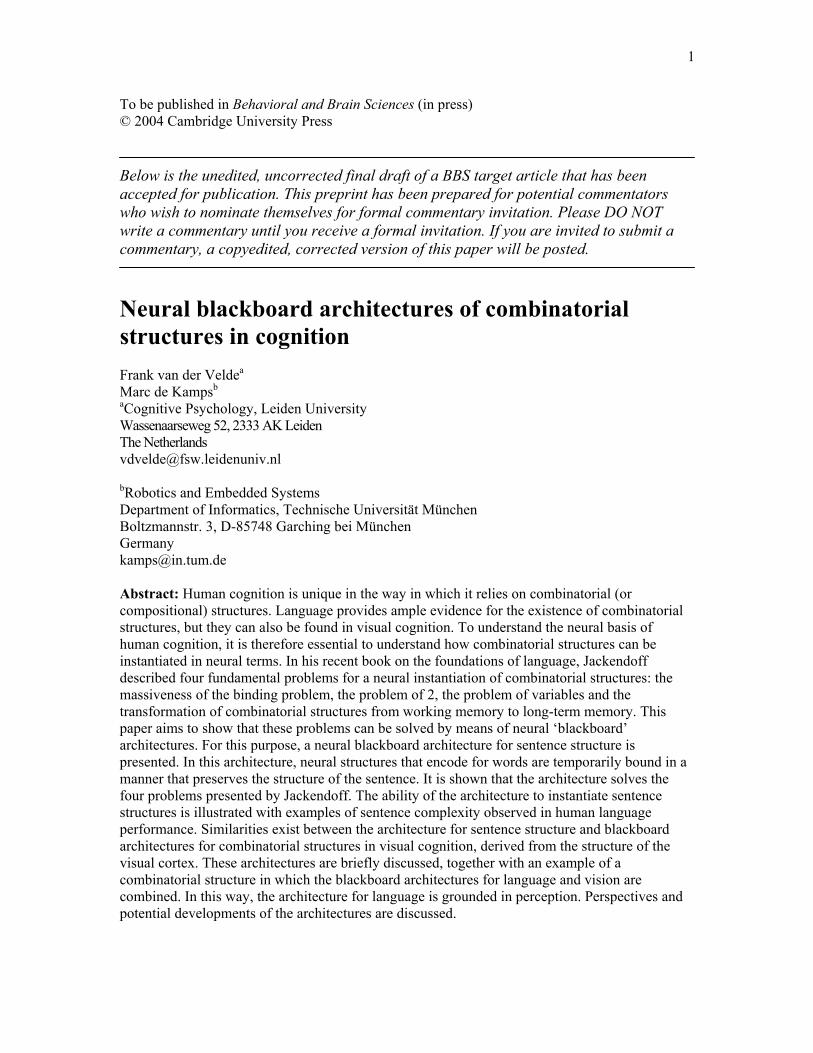
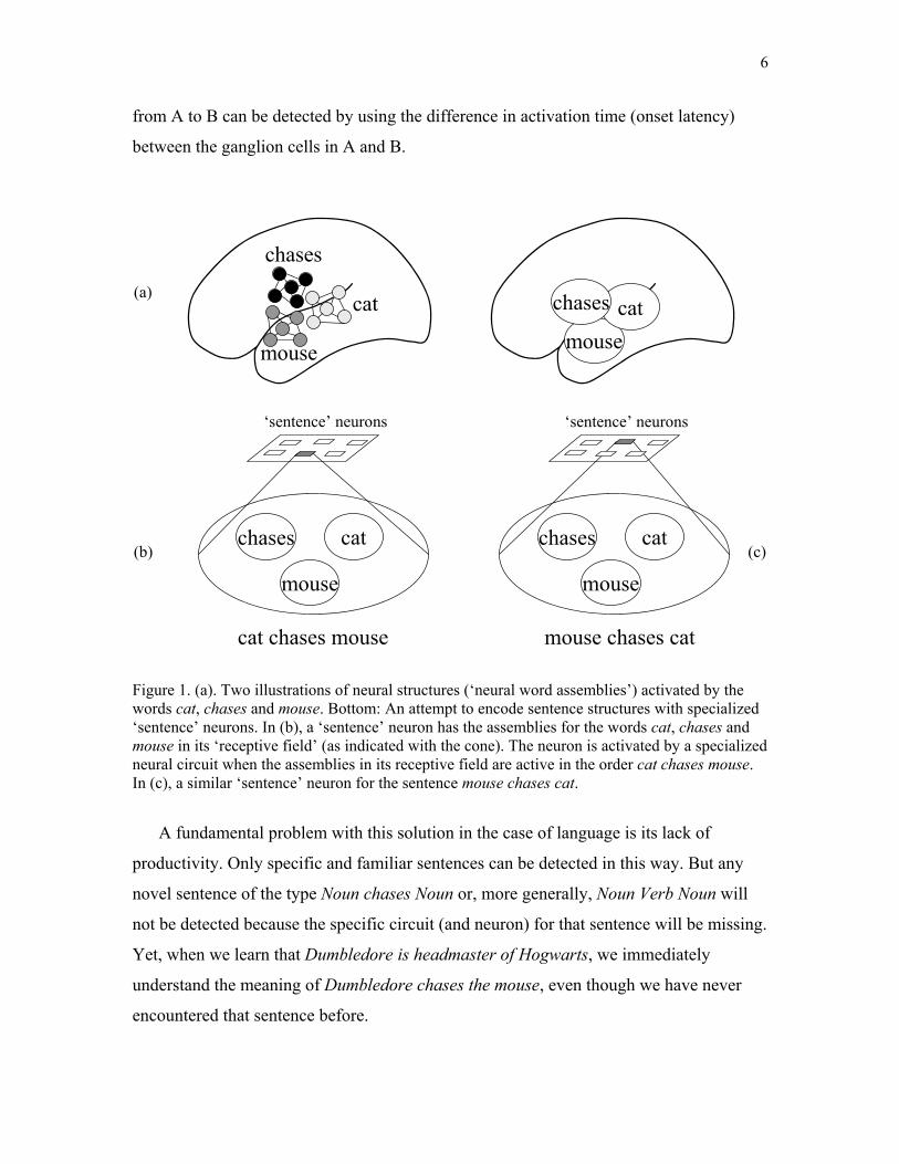
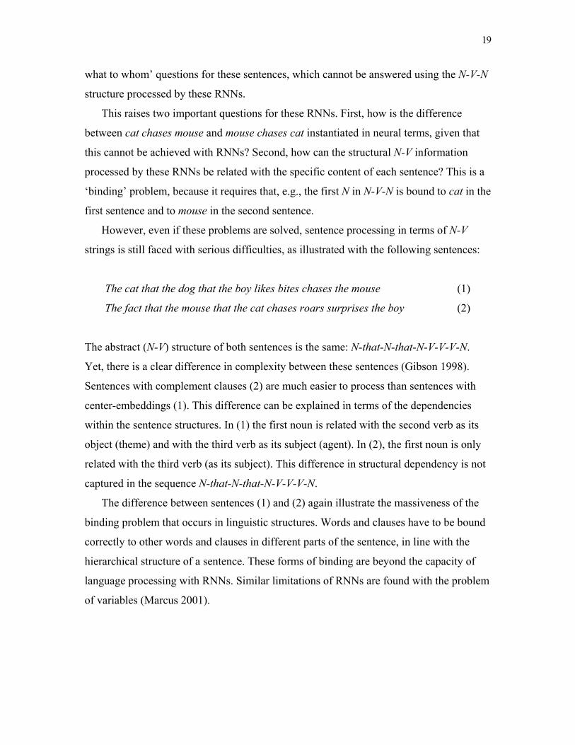
In the case of language, the problem is illustrated in figure 1. Assume that words like
cat, chases and mouse each activate specific neural structures, such as the ‘word
assemblies’ discussed by Pulvermüller (1999). The problem is how the neural structures
or word assemblies for cat and mouse can be bound to the neural structure or word
assembly of the verb chases, in line with the thematic roles (or argument structure) of the
verb. That is, how cat and mouse can be bound to the role of agent and theme of chases
in the sentence The cat chases the mouse, and to the role of theme and agent of chases in
the sentence The mouse chases the cat.
A potential solution for this problem is illustrated in figure 1. It consists of
specialized neurons (or populations of neurons) that are activated when the strings cat
chases mouse (figure 1b) or mouse chases cat (figure 1c) are heard or seen. Each neuron
has the word assemblies for cat, mouse and chases in its ‘receptive field’ (illustrated with
the cones in figures 1b and 1c). Specialized neural circuits could activate one neuron in
the case of cat chases mouse and the other neuron in the case of mouse chases cat, by
using the difference in temporal word order in both strings. Circuits of this kind can be
found in the case of motion detection in visual perception (e.g., Hubel 1995). For
instance, the movement of a vertical bar that sweeps across the retina in the direction
6
from A to B can be detected by using the difference in activation time (onset latency)
between the ganglion cells in A and B.
Figure 1. (a). Two illustrations of neural structures (‘neural word assemblies’) activated by the words cat, chases and mouse. Bottom: An attempt to encode sentence structures with specialized ‘sentence’ neurons. In (b), a ‘sentence’ neuron has the assemblies for the words cat, chases and mouse in its ‘receptive field’ (as indicated with the cone). The neuron is activated by a specialized neural circuit when the assemblies in its receptive field are active in the order cat chases mouse. In (c), a similar ‘sentence’ neuron for the sentence mouse chases cat.
A fundamental problem with this solution in the case of language is its lack of
productivity. Only specific and familiar sentences can be detected in this way. But any
novel sentence of the type Noun chases Noun or, more generally, Noun Verb Noun will
not be detected because the specific circuit (and neuron) for that sentence will be missing.
Yet, when we learn that Dumbledore is headmaster of Hogwarts, we immediately
understand the meaning of Dumbledore chases the mouse, even though we have never
encountered that sentence before.
mouse chases catcat chases mouse
mousecat
mouse
chases cat
(a)
(b) (c)
chases
mouse
chases cat
‘sentence’ neurons ‘sentence’ neurons
chases
cat
mouse

7
The difference between language and motion detection in this respect illustrates that
the nature of these two cognitive processes is fundamentally different. In the case of
motion detection there is a limited set of possibilities, so that it is possible (and it pays
off) to have specialized neurons and neural circuits for each of these possibilities. But this
solution is not feasible in the case of language. Linguists typically describe language in
terms of its unlimited combinatorial productivity. Words can be combined into phrases,
which in turn can be combined into sentences, so that arbitrary sentence structures can be
filled with arbitrary arguments (e.g., Webelhuth 1995; Sag & Wasow 1999; Chomsky
2000; Pullum & Scholz 2001; Jackendoff 2002; Piattelli-Palmarini 2002). In theory, an
unlimited amount of sentences can be produced in this way, which excludes the
possibility of having specialized neurons and circuits for each of these sentences.
However, unlimited (recursive) productivity is not necessary to make a case for the
combinatorial nature of language, given the number of sentences that can be produced or
understood. For instance, the average English-speaking 17-year-old knows more than
60.000 words (Bloom 2000). With this lexicon, and with a limited sentence length of 20
words or less, one can produce a set of sentences in natural language in the order of 1020
or more (Miller 1967; Pinker 1998). A set of this kind can be characterized as a
‘performance set’ of natural language, in the sense that (barring a few selected examples)
any sentence from this set can be produced or understood by a normal language user.
Such a performance set is not unlimited, but it is of ‘astronomical’ magnitude (e.g., 1020
exceeds the estimated lifetime of the universe expressed in seconds). By consequence,
most sentences in this set are sentences that we have never heard or seen before. Yet,
because of the combinatorial nature of language, we have the ability to produce and
understand arbitrary sentences from a set of this kind.
Hence, the set of possibilities that we can encounter in the case of language is
unlimited in any practical sense. This precludes a solution of the binding problem in
language in terms of specialized neurons and circuits. Instead, a solution is needed that
depends on the ability to bind arbitrary arguments to the thematic roles of arbitrary verbs,
in agreement with the structural relations expressed in the sentence. Moreover, the
solution has to satisfy the massiveness of the binding problem as it occurs in language,
which is due to the often complex and hierarchical nature of linguistic structures. For

8
instance, in the sentence The cat that the dog bites chases the mouse, the noun cat is
bound to the role of theme of the verb bites, but it is bound to the role of agent of the verb
chases. In fact, the whole phrase The cat that the dog bites is bound to the role of agent of
the verb chases (with cat as the head of the phrase). Each of these specific bindings has to
be satisfied in an encoding of this sentence.
2.2. The problem of 2
The second problem presented by Jackendoff (2002) is the problem of multiple instances,
or the ‘problem of 2’. Jackendoff illustrates this problem with the sentence The little star
is beside a big star2. The word star occurs twice in this sentence, the first time related
with the word little and the second time related with the word big. The problem is how in
neural terms the two occurrences of the word star can be distinguished, so that star is
first bound with little and then with big, without creating the erroneous binding of little
big star. The problem of 2 results from the assumption that any occurrence of a given
word will result in the activation of the same neural structure (e.g., its word assembly, as
illustrated in figure 1). But if the second occurrence of a word only results in the
reactivation of a neural structure that was already activated by the first occurrence of that
word, the two occurrences of the same word are indistinguishable (Van der Velde 1999).
Perhaps the problem could be solved by assuming that there are multiple neural
structures that encode for a single word. The word star could then activate one neural
structure in little star and a different one in big star, so that the bindings little star and big
star can be encoded without creating little big star. However, this solution would entail
that there are multiple neural structures for all words in the lexicon, perhaps even for all
potential positions a word could have in a sentence (Jackendoff 2002).
More importantly even, this solution disrupts the unity of word encoding as the basis
for the meaning of a word. For instance, the relation between the neural structures for cat
and mouse in cat chases mouse could develop into the neural basis for the long-term
knowledge (‘fact’) that cats chase mice. Similarly, the relation between the neural
structures for cat and dog in dog bites cat could form the basis of the fact that dogs fight
9
with cats. But if the neural structure for cat (say, cat1) in cat1 chases mouse is different
from the neural structure for cat (say, cat2) in dog bites cat2, then these two facts are
about different kinds of animals.
2.2.1. The problem of 2 and the symbol grounding problem
It is interesting to look at the problem of 2 from the perspective of the symbol grounding
problem that occurs in cognitive symbol systems. Duplicating symbols is easy in a
symbol system. However, in a symbol system, one is faced with the problem that
symbols are arbitrary entities (e.g., strings of bits in a computer), which therefore have to
be interpreted to provide meaning to the system. That is, symbols have to be ‘grounded’
in perception and action if symbol systems are to be viable models of cognition (Harnad
1991; Barsalou 1999).
Grounding in perception and action can be achieved with neural structures such as the
word assemblies illustrated in figure 1. In line with the idea of neural assemblies
proposed by Hebb (1949), Pulvermüller (1999) argued that words activate neural
assemblies, distributed over the brain (as illustrated with the assemblies for the words cat,
mouse and chases in figure 1). One could imagine that these word assemblies have
developed over time by means of a process of association. Each time a word was heard or
seen, certain neural circuits would have been activated in the cortex. Over time, these
circuits will be associated, which results in an overall cell assembly that reflects the
meaning of that word.
But, as argued above, word assemblies are faced with the problem of 2. Thus, it
seems that the problem of 2 and the symbol grounding problem are complementary
problems. To provide grounding, the neural structure that encodes for a word is
embedded in the overall network structure of the brain. But this makes it difficult to
instantiate a duplication of the word, and thus to instantiate even relatively simple
combinatorial structures such as The little star is beside a big star. Conversely,
duplication is easy in symbol systems (e.g., if ‘1101’ = star, then one would have The
little 1101 is beside a big 1101, with little and big each related to an individual copy of
1101). But symbols can be duplicated easily because they are not embedded in an overall
structure that provides the grounding of the symbol3.
10
2.3. The problem of variables
The knowledge of specific facts can be instantiated on the basis of specialized neural
circuits, in line with those illustrated in figure 1. But knowledge of systematic facts, such
as the fact that own(y,z) follows from give(x,y,z), cannot be instantiated in this way, that
is, in terms of a listing of all specific instances of the relation between the predicates own
and give (e.g., from give(John, Mary, book) it follows that own(Mary, book); from
give(Mary, John, pen) it follows that own(John, pen); etc.).
Instead, the derivation that own(Mary, book) follows from give(John, Mary, book) is
based on the rule that own(y,z) follows from give(x,y,z), combined with the binding of
Mary to the variable y and book to the variable z. Marcus (2001) analyzed a wide range of
relationships that can be described in this way. They are all characterized by the fact that
an abstract rule-based relationship, expressed in terms of variables, is used to determine
relations between specific entities (e.g., numbers, words, objects, individuals).
The use of rule-based relationships with variable binding provides the basis for the
systematic nature of cognition (Fodor & Pylyshyn 1988). Cognition is systematic in the
sense that one can learn from specific examples and apply that knowledge to all examples
of the same kind. A child will indeed encounter only specific examples (e.g., that when
John gives Mary a book, it follows that Mary owns the book) and yet it will learn that
own(y,z) follows from all instances of the kind give(x,y,z). In this way, the child is able to
handle novel situations, such as the derivation that own(Harry, broom) follows from
give(Dumbledore, Harry, broom).
The importance of rule-based relationships for human cognition raises the question of
how relationships with variable binding can be instantiated in the brain.
2.4. Binding in working memory versus long-term memory
Working memory in the brain is generally assumed to consist of a sustained form of
activation (e.g, Amit 1989; Fuster 1995). That is, information is stored in working
memory as long as the neurons that encode the information remain active. In contrast,
long-term memory results from synaptic modification, such as long-term potentiation
(LTP). In this way, the connections between neurons are modified (e.g., enhanced). When

11
some of the neurons are then reactivated, they will reactivate the others neurons as well.
The neural word assemblies, illustrated in figure 1, are formed by this process.
Both forms of memory are related in the sense that information in one form of
memory can be transformed into information in the other form of memory. Information
could be stored in a working memory (which could be specific for a given form of
information, such as sentence structures) before it is stored in long-term memory.
Conversely, information in long-term memory can be reactivated and stored in working
memory. This raises the question of how the same combinatorial structure can be
instantiated both in terms of neural activation (as found in working memory or in
stimulus dependent activation) and in terms of synaptic modification, and how these
different forms of instantiation can be transformed into one another.
2.5. Overview
It is clear that the four problems presented by Jackendoff (2002) are interrelated. For
instance, the problem of 2 also occurs in rule-based derivation with variable binding, the
massiveness of the binding problem is found in combinatorial structures stored in
working memory and in combinatorial structures stored in long-term memory. Therefore,
a solution of these problems has to be an integrated one that solves all four problems
simultaneously. In this paper, we will discuss how all four problems can be solved in
terms of neural blackboard architectures in which combinatorial structures can be
instantiated.
First, however, we will discuss two alternatives for a neural instantiation of
combinatorial structures: the use of synchrony of activation (e.g., Von der Malsburg
1987) as a mechanism for binding constituents in combinatorial structures, and the use of
recurrent neural networks to process combinatorial structures, in particular sentence
structures.
3. Combinatorial structures with synchrony of activation
An elaborate example of a neural instantiation of combinatorial structures in which
synchrony of activation is used as a binding mechanism is found in the model of reflexive
reasoning presented by Shastri and Ajjanagadde (1993). In their model, synchrony of
12
activation is used to show how a known fact such as John gives Mary a book can result in
an inference such as Mary owns a book.
The proposition John gives Mary a book is encoded by a ‘fact node’ that detects the
respective synchrony of activation between the nodes for John, Mary and book, and the
nodes for giver, recipient and give-object, which encode for the thematic roles of the
predicate give(x,y,z). In a simplified manner, the reasoning process begins with the query
own(Mary, book)? (i.e., does Mary own a book?). The query results in the respective
synchronous activation of the nodes for owner and own-object of the predicate own(y,z)
with the nodes for Mary and book. In turn, the nodes for recipient and give-object of the
predicate give(x,y,z) are activated by the nodes for owner and own-object, such that
owner is in synchrony with recipient and own-object is in synchrony with give-object. As
a result, the node for Mary is in synchrony with the node for recipient and the node for
book is in synchrony with the node for give-object. This allows the fact node for John
gives Mary a book to become active, which produces the affirmative answer to the query.
A first problem with a model of this kind is found in a proposition like John gives
Mary a book and Mary gives John a pen. With synchrony of activation as a binding
mechanism, a confusion arises between John and Mary in their respective roles of giver
and recipient in this proposition. In effect, the same pattern of activation will be found in
the proposition John gives Mary a pen and Mary gives John a book. Thus, with
synchrony of activation as a binding mechanism, both propositions are indistinguishable.
It is not difficult to see the problem of 2 here. John and Mary occur twice in the
proposition, but in different thematic roles. The simultaneous but distinguishable binding
of John and Mary with different thematic roles cannot be achieved with synchrony of
activation.
To solve this problem, Shastri and Ajjanagadde allowed for a duplication (or
multiplication) of the nodes for the predicates. In this way, the whole proposition John
gives Mary a book and Mary gives John a pen is partitioned into the two elementary
propositions John gives Mary a book and Mary gives John a pen. To distinguish between
the propositions, the nodes for the predicate give(x,y,z) are duplicated. Thus, there are
specific nodes for, say, give1(x,y,z) and give2(x,y,z), with give1(x,y,z) related with John
gives Mary a book and give2(x,y,z) related with Mary gives John a pen. Furthermore, for
13
the reasoning process to work, the associations between predicates have to be duplicated
as well. Thus, the node for give1(x,y,z) has to be associated with a node for, say, own1(y,z)
and the node for give2(x,y,z) has to be associated with a node for own2(y,z).
This raises the question of how these associations can be formed simultaneously
during learning. During its development, a child will learn from specific examples. Thus,
it will learn that, when John gives Mary a book, it follows that Mary owns the book. In
this way, the child will form an association between the nodes for give1(x,y,z) and
own1(y,z). But the association between the node for give2(x,y,z) and own2(y,z) would not
be formed in this case, because these nodes are not activated with John gives Mary a
book and Mary owns the book. Thus, when the predicate give(x,y,z) is duplicated into
give1(x,y,z) and give2(x,y,z), the systematicity between John gives Mary a book and Mary
gives John a pen is lost.
3.1. Nested structures with synchrony of activation
The duplication solution discussed above fails with nested (or hierarchical) propositions.
For instance, the proposition Mary knows that John knows Mary cannot be partitioned
into two propositions Mary knows and John knows Mary, because the entire second
proposition is the y argument of knows(Mary, y). Thus, the fact node for John knows
Mary has to be in synchrony with the node for know-object of the predicate know(x,y).
The fact node for John knows Mary will be activated because John is in synchrony with
the node for knower and Mary is in synchrony with the node for know-object. However,
the fact node for Mary knows Mary, for instance, will also be activated in this case,
because Mary is in synchrony with both knower and know-object in the proposition Mary
knows that John knows Mary. Thus, the proposition Mary knows that John knows Mary
cannot be distinguished from the proposition Mary knows that Mary knows Mary.
As this example shows, synchrony as a binding mechanism is faced with the ‘one-
level’ restriction (Hummel & Holyoak, 1993), i.e., synchrony can only encode bindings
at one level of abstraction or hierarchy at a time.
14
3.2. Productivity with synchrony of activation
A fundamental problem with the use of synchrony of activation as a binding mechanism
in combinatorial structures is its lack of productivity. Synchrony of activation has to be
detected to process the information that it encodes (Dennett 1991). In Shastri and
Ajjanagadde’s model, fact nodes (e.g., the fact node for John gives Mary a book) detect
the synchrony of activation between arguments and thematic roles. But fact nodes, and
the circuits that activate them, are similar to the specialized neurons and circuits
illustrated in figure 1. It is excluded to have such nodes and circuits for all possible verb-
argument bindings that can occur in language, in particular for novel instances of verb-
argument binding. As a result, synchrony of activation as a binding mechanism fails to
provide the productivity given by combinatorial structures.
The binding problems as analyzed here, the inability to solve the problem of 2, the
inability to deal with nested structures (the ‘one-level restriction’), and the lack of
systematicity and productivity, are typical for the use of synchrony of activation as a
binding mechanism (Van der Velde & de Kamps 2002a). The lack of productivity, given
by the need for ‘synchrony detectors’, is perhaps the most fundamental problem for
synchrony as a mechanism for binding constituents in combinatorial structures. True
combinatorial structures provide the possibility to answer binding questions about novel
combinations (e.g., novel sentences) never seen or heard before. Synchrony detectors (or
conjunctive forms of encoding in general) will be missing for novel combinatorial
structures, which precludes the use of synchrony as a binding mechanism for these
structures. Synchrony as a binding mechanism would seem to be restricted to structures
for which conjunctive forms of encoding exist, and which satisfy the ‘one-level
restriction’ (Van der Velde & de Kamps 2002a).
4. Processing linguistic structures with ‘simple’ recurrent neural networks
The argument that combinatorial structures are needed to obtain productivity in cognition
has been questioned (Elman 1991; Churchland 1995, Port & Van Gelder 1995). In this
view, productivity in cognition can be obtained in a ‘functional’ manner (‘functional
compositionality’, Van Gelder 1990), without relying on combinatorial structures. The
most explicit models of this kind deal with sentence structures.

15
A first example is the neural model of thematic role assignment in sentence
processing presented by McClelland and Kawamoto (1986). However, the model was
restricted to one particular sentence structure, and it could not represent different tokens
of the same type, e.g., dogagent and dogtheme in dog chases dog. St.John and McClelland
(1990) presented a more flexible model based on a recurrent network. The model learned
pre-segmented single-clause sentences and assigned thematic roles to the words in the
sentence, but it could not handle more complex sentences, like sentences with embedded
clauses.
A model that processed embedded clauses was presented by Miikkulainen (1996). It
consisted of three parts: a parser, a segmenter and a stack. The segmenter (a feedforward
network) divided the input sentence into clauses (by detecting clause boundaries). The
stack memorized the beginning of a matrix clause, e.g., girl in The girl, who liked the
boy, saw the boy. The parser that assigned thematic roles (agent, act, patient) to the words
in a clause. All clauses, however, were two or three word clauses, because the output
layer of the parser had three nodes.
The ‘simple’ recurrent neural networks (RNNs for short) play an important role in the
attempt to process sentence structures without relying on combinatorial structures (Elman
1991; Miikkulainen 1996; Palmer-Brown et al. 2002). They consist of a multilayer
feedforward network, in which the activation pattern in the hidden (middle) layer is
copied back to the input layer, as part of the input to the network in the next learning step.
In this way, RNNs are capable of processing sequential structures. Elman (1991) used
RNNs in a word prediction task. For instance, with Boys who chase boy feed cats, the
network had to predict that after Boys who chase a noun would follow, and that after
Boys who chase boy a plural verb would occur. The network was trained with sentences
from a language generated with a small lexicon and a basic phrase grammar. The network
succeeded in this task, both for the sentences that were used in the training session and
with other sentences from the same language.
The RNNs used by Elman (1991) could not answer specific binding questions like
"Who feed cats?”. Thus, the network did not bind specific words to their specific roles in
the sentence structure. Nevertheless, RNNs seem capable of processing aspects of
sentence structures in a noncombinatorial manner. But RNNs model languages derived
16
from small vocabularies (in the order of 10 to 100 words). In contrast, the vocabulary of
natural language is huge, which results in an ‘astronomical’ productivity, even with
limited sentence structures (e.g., sentences with 20 words or less, see section 2.1.). We
will discuss ‘combinatorial’ productivity with RNNs in more detail.
4.1. Combinatorial productivity with RNNs used in sentence processing
Elman (1991) used a language in the order of 105 sentences, based on a lexicon of about
20 words. In contrast, the combinatorial productivity of natural language is in the order of
1020 sentences or more, based on a lexicon of 105 words. A basic aspect of such a
combinatorial productivity is the ability to insert words from one familiar sentence
context into another. For instance, if one learns that Dumbledore is headmaster of
Hogwarts, one can also understand Dumbledore chases the mouse even though this
specific sentence has not been encountered before. To approach the combinatorial
productivity of natural language, RNNs should have this capability as well.
We investigated this question by testing the ability of RNNs to recognize a sentence
consisting of a new combination of familiar words in familiar syntactic roles (Van der
Velde et al. 2004a). In one instance, we used sentences like dog hears cat, boy sees girl,
dog loves girl and boy follows cat to train the network on the word prediction task. The
purpose of the training sentences was to familiarize the RNNs with dog, cat, boy and girl
as arguments of verbs. Then, a verb like hears from dog hears cat was inserted into
another trained sentence like boy sees girl to form the test sentence boy hears girl, and
the networks were tested on the prediction task for this sentence.
To strengthen the relations between boy, hears and girl, we also included training
sentences like boy who cat hears obeys John and girl who dog hears likes Mary. These
sentences introduce boy and hears, and girl and hears, in the same sentence context
(without using boy hears and hears girl)4. In fact, girl is the object of hears in girl who
dog hears likes Mary, as in the test sentence boy hears girl.
However, although the RNNs learned the training sentences to perfection, they failed
with the test sentences. Despite the ability to process boy sees girl and dog hears cat, and
even girl who dog hears likes Mary, they could not process boy hears girl. The behavior
of the RNNs with the test sentence boy hears girl was similar to the behavior in a ‘word

17
salad’ condition, which consisted of random word strings based on the words used in the
training session. In this ‘word salad’ condition the RNNs predicted the next word on the
basis of direct word-word associations, determined by all two-word combinations found
in the training sentences. The similarity between ‘word salads’ and the test sentence boy
hears girl suggests that RNNs resort to word-word associations when they have to
process novel sentences composed of familiar words in familiar grammatical structures.
The results of these simulations indicate that RNNs of Elman (1991) do not posses a
minimal form of the combinatorial productivity underlying human language processing.
It is important to note that this lack of combinatorial productivity is not just a negative
result, that resulted from the learning algorithm used. The training sentences were learned
to perfection. With another algorithm, these sentences could, at best, be learned to the
same level of perfection. Furthermore, the crucial issue here is not learning, but the
contrast in behavior exhibited by the RNNs in these simulations. The RNNs were able to
process (‘understand’) boy sees girl and dog hears cat, and even girl who dog hears likes
Mary, but not boy hears girl. This contrast in behavior is not found in humans, regardless
of the learning procedure used. The reason is the systematicity of the human language
system. If you understand boy sees girl, dog hears cat and girl who dog hears likes Mary,
you cannot but understand boy hears girl. Any failure to do so would be regarded as
pathological5.
4.2. Combinatorial productivity versus recursive productivity
The issue of combinatorial productivity is a crucial aspect of natural language processing,
which is sometimes confused with the issue of recursive productivity. Combinatorial
productivity concerns the productivity that results from combining a large lexicon with
even limited syntactical structures. Recursive productivity deals with the issue of
processing more complex syntactic structures, such as (deeper) center-embeddings.
The difference can be illustrated with the ‘long short-term memory recurrent
networks’ (LSTMs). LSTMs outperform standard RNNs on recursive productivity (Gers
& Schmidhuber, 2001). Like humans, RNNs have limited recursive productivity, but
LSTMs do not. They can, e.g., handle context-free languages like anbmBmAn for arbitrary
18
(n,m). However, the way in which they do this excludes their ability to handle
combinatorial productivity.
A LSTM is a RNN in which hidden units are replaced with "memory blocks" of units,
which develop into counters during learning. With anbmBmAn , the network develops two
counters, one for n’s and one for the m’s. Thus, the network counts whether an matches
An and bm matches Bm. This makes sense because all sentences have the same words, i.e.,
they are all of the form anbmBmAn. Sentences differ only in the value of n and/or m. So,
the network can learn that it has to count the n’s and m’s.
But this procedure makes no sense in a natural language. A sentence mouse chases
cat is fundamentally different from the sentence cat chases mouse, even though they are
both Noun-Verb-Noun sentences. How could a LSTM capture this difference? Should the
model, e.g., count the number of times that mouse and cat appear in any given sentence?
Consider the number of possibilities that would have to be dealt with, given a lexicon of
60.000 words, instead of four words as in anbmBmAn . Furthermore, how would deal with
novel sentences, like Dumbledore chases mouse? Could it have developed counters to
match Dumbledore and mouse if it has never seen these words in one sentence before?
This example illustrates that combinatorial productivity is an essential feature of
natural language processing, but virtually non-existent in artificial languages. The ability
to process complex artificial languages does not guarantee the ability to process
combinatorial productivity as found in natural language.
4.3. RNNs and the massiveness of the binding problem
Yet RNNs are capable of processing learned sentences like girl who dog hears obeys
Mary, and other complex sentence structures. Perhaps RNNs could be used to process
sentence structures in abstract terms, i.e., in terms of Nouns (N) and Verbs (V). Thus, N-
who-N-V-V-N instead of girl who dog hears obeys Mary.
However, sentences like cat chases mouse and mouse chases cat are N-V-N sentences,
and thus indistinguishable for these RNNs. But these sentences convey very different
messages, which humans can understand. In particular, humans can answer ‘who does
19
what to whom’ questions for these sentences, which cannot be answered using the N-V-N
structure processed by these RNNs.
This raises two important questions for these RNNs. First, how is the difference
between cat chases mouse and mouse chases cat instantiated in neural terms, given that
this cannot be achieved with RNNs? Second, how can the structural N-V information
processed by these RNNs be related with the specific content of each sentence? This is a
‘binding’ problem, because it requires that, e.g., the first N in N-V-N is bound to cat in the
first sentence and to mouse in the second sentence.
However, even if these problems are solved, sentence processing in terms of N-V
strings is still faced with serious difficulties, as illustrated with the following sentences:
The cat that the dog that the boy likes bites chases the mouse (1)
The fact that the mouse that the cat chases roars surprises the boy (2)
The abstract (N-V) structure of both sentences is the same: N-that-N-that-N-V-V-V-N.
Yet, there is a clear difference in complexity between these sentences (Gibson 1998).
Sentences with complement clauses (2) are much easier to process than sentences with
center-embeddings (1). This difference can be explained in terms of the dependencies
within the sentence structures. In (1) the first noun is related with the second verb as its
object (theme) and with the third verb as its subject (agent). In (2), the first noun is only
related with the third verb (as its subject). This difference in structural dependency is not
captured in the sequence N-that-N-that-N-V-V-V-N.
The difference between sentences (1) and (2) again illustrate the massiveness of the
binding problem that occurs in linguistic structures. Words and clauses have to be bound
correctly to other words and clauses in different parts of the sentence, in line with the
hierarchical structure of a sentence. These forms of binding are beyond the capacity of
language processing with RNNs. Similar limitations of RNNs are found with the problem
of variables (Marcus 2001).
20
5. Blackboard architectures of combinatorial structures
A combinatorial structure consists of parts (constituents) and their relations. The lack of
combinatorial productivity with RNNs illustrates a failure to encode the individual parts
(words) of a combinatorial structure (sentence) in a productive manner. In contrast,
synchrony of activation fails to instantiate even moderately complex relations in the case
of variable binding. These examples show that neural models of combinatorial structures
can only succeed if they provide a neural instantiation of both the parts and the relations
of combinatorial structures.
A blackboard architecture provides a way to instantiate the parts and the relations of
combinatorial structures (e.g., Newman et al. 1997). A blackboard architecture consists of
a set of specialized processors (‘demons’, Selfridge 1959) that interact with each other
using a blackboard (‘workbench’, ‘bulletin board’). Each processor can process and
modify the information stored on the blackboard. In this way, the architecture exceeds the
ability of each individual processor. For language, one could have processors for the
recognition of words and for the recognition of specific grammatical relations. These
processors could then interact by using a blackboard to process a sentence. With the
sentence The little star is beside a big star, the word processors could store the symbol
for star on the blackboard, first in combination with the symbol for little, and then in
combination with the symbol for big. Other processors could determine the relation
(beside) between these two copies of the symbol for star. Jackendoff (2002) discusses
blackboard architectures for phonological, syntactic and semantic structures.
Here, we will propose and discuss a neural blackboard architecture for sentence
structure based on neural assemblies. To address Jackendoff’s (2002) problems, neural
word assemblies are not copied in this architecture. Instead, they are temporarily bound
to the neural blackboard, in a manner that distinguishes between different occurrences of
the same word, and that preserves the relations between the words in the sentence. For
instance, with the sentence The cat chases the mouse, the neural assemblies for cat and
mouse are bound to the blackboard as the subject (agent) and object (theme) of chases.
With the neural structure of The cat chases the mouse, the architecture can produce
correct answers to questions like “Who chases the mouse?” or “Whom does the cat
chase?”. These questions can be referred to as ‘binding questions’, because they test the
21
ability of an architecture to ‘bind’ familiar parts in a (potentially novel) combinatorial
structure. A neural instantiation of a combinatorial structure like The cat chases the
mouse fails if it cannot produce the correct answers to such questions. In language,
binding questions typically query ‘who does what to whom’ information, which is
characteristic of information provided by a sentence (Pinker 1994; Calvin & Bickerton
2000). Aphasic patients, for instance, are tested on their language abilities using non-
verbal ‘who does what to whom’ questions (Caplan 1992). In general, the ability to
answer binding questions is of fundamental importance for cognition, because it is related
with the ability to select information needed for purposive action (Van der Heijden & van
der Velde 1999).
6. A neural blackboard architecture of sentence structure
In the architecture, words are encoded in terms of neural ‘word’ assemblies, in line with
Pulvermüller (1999), as illustrated in figure 1. It is clear that the relations between the
words in a sentence cannot be encoded by direct associations between word assemblies.
For instance, the association cat-chases-mouse does not distinguish between The cat
chases the mouse and The mouse chases the cat.
However, relations between words can be encoded, and Jackendoff ‘s problems can
be solved, if word assemblies are embedded in a neural architecture in which structural
relations can be formed between these assemblies. Such an architecture can be formed by
combining word assemblies with ‘structure’ assemblies.
A word assembly is a neural structure that is potentially distributed over a large part
of the brain, depending on the nature of the word (e.g., see Pulvermüller 1999). A part of
that structure could be embedded in a ‘phonological’ architecture that controls the
auditory perception and speech production related with that word. Other parts could be
embedded in other architectures that control other forms of neural processing related with
other aspects of that word (e.g., visual perception, semantics).
Here, we propose that a part of a word assembly is embedded in a neural architecture
for sentence structure, given by ‘structure’ assemblies and their relations. A word
assembly can be associated (‘bound’) temporarily with a given structure assembly, so that
it is (temporarily) ‘tagged’ by the structure assembly to which it is bound. A word
22
assembly can be bound simultaneously with two or more structure assemblies. The
different structure assemblies provide different ‘tags’ for the word assembly, which
distinguish between different ‘copies’ of the word encoded with the word assembly.
However, the word assembly itself is not ‘copied’ or disrupted in this process, and its
associations and relations remain intact when a word assembly is tagged by a given
structure assembly. Thus, any ‘copy’ of a word is always ‘grounded’ (as discussed in
section 2.2.1).
Structure assemblies are selective. For instance, nouns and verbs bind to different
kinds of structure assemblies. Furthermore, the internal structure of structure assemblies
allows selective activation of specific parts within each structure assembly. Structure
assemblies of a given kind can selectively bind temporarily to specific other structure
assemblies, so that a (temporal) neural structure of a given sentence is created. Thus,
structure assemblies can encode different instantiations of the same word assembly
(solving the ‘problem of 2’), and they can bind word assemblies in line with the syntactic
structure of the sentence.
Binding in the architecture occurs between word assemblies and structure assemblies,
and between structure assemblies. Binding between two assemblies derives from
sustained (‘delay’) activity in a connection structure that links the two assemblies. This
activity is initiated when the two assemblies are concurrently active. The delay activity is
similar to the sustained activation found in the ‘delay period’ in working memory
experiments (e.g., Durstewitz et al. 2000). Two assemblies are bound as long as this
delay activity continues.
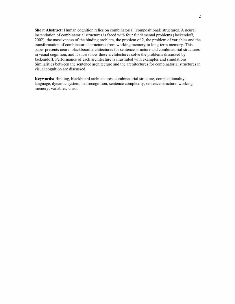
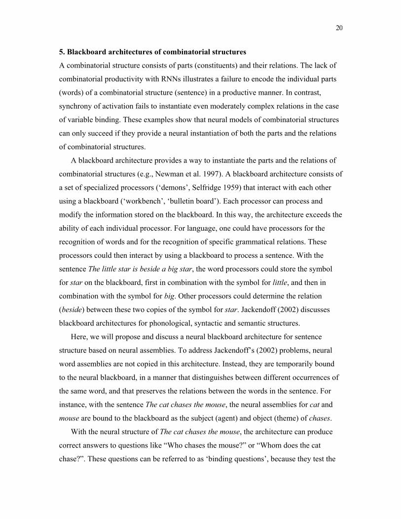
Figure 2 illustrates the basic neural structure in the architecture of cat chases mouse.
The structure consists of the word assemblies of cat, mouse and chases, and structure
assemblies for noun phrases (NPs) and verb phrases (VPs), together with ‘gating circuits’
and ‘memory circuits’. Gating circuits are used to selectively activate specific parts
within structure assemblies. Memory circuits are used to bind two assemblies
temporarily.
The assemblies for cat and mouse are bound to two different NP assemblies (N1 and
N2), and the assembly for chases is bound a VP assembly (V1). The structure assemblies
are bound to each other, to encode the verb-argument structure of the sentence. For this
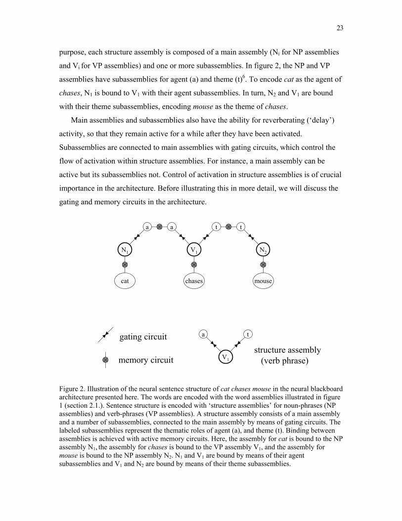
23
purpose, each structure assembly is composed of a main assembly (Ni for NP assemblies
and Vi for VP assemblies) and one or more subassemblies. In figure 2, the NP and VP
assemblies have subassemblies for agent (a) and theme (t)6. To encode cat as the agent of
chases, N1 is bound to V1 with their agent subassemblies. In turn, N2 and V1 are bound
with their theme subassemblies, encoding mouse as the theme of chases.
Main assemblies and subassemblies also have the ability for reverberating (‘delay’)
activity, so that they remain active for a while after they have been activated.
Subassemblies are connected to main assemblies with gating circuits, which control the
flow of activation within structure assemblies. For instance, a main assembly can be
active but its subassemblies not. Control of activation in structure assemblies is of crucial
importance in the architecture. Before illustrating this in more detail, we will discuss the
gating and memory circuits in the architecture.
Figure 2. Illustration of the neural sentence structure of cat chases mouse in the neural blackboard architecture presented here. The words are encoded with the word assemblies illustrated in figure 1 (section 2.1.). Sentence structure is encoded with ‘structure assemblies’ for noun-phrases (NP assemblies) and verb-phrases (VP assemblies). A structure assembly consists of a main assembly and a number of subassemblies, connected to the main assembly by means of gating circuits. The labeled subassemblies represent the thematic roles of agent (a), and theme (t). Binding between assemblies is achieved with active memory circuits. Here, the assembly for cat is bound to the NP assembly N1, the assembly for chases is bound to the VP assembly V1, and the assembly for mouse is bound to the NP assembly N2. N1 and V1 are bound by means of their agent subassemblies and V1 and N2 are bound by means of their theme subassemblies.
N1
cat
V1
a a
chases
N2
t t
mouse
memory circuitstructure assembly
(verb phrase)
gating circuit
V1
a t
24
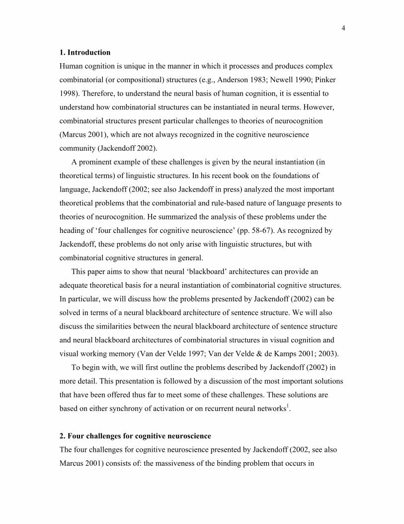
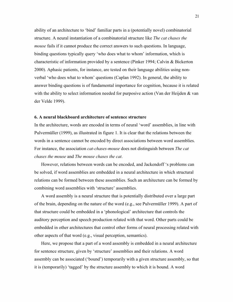
6.1. Gating and memory circuits
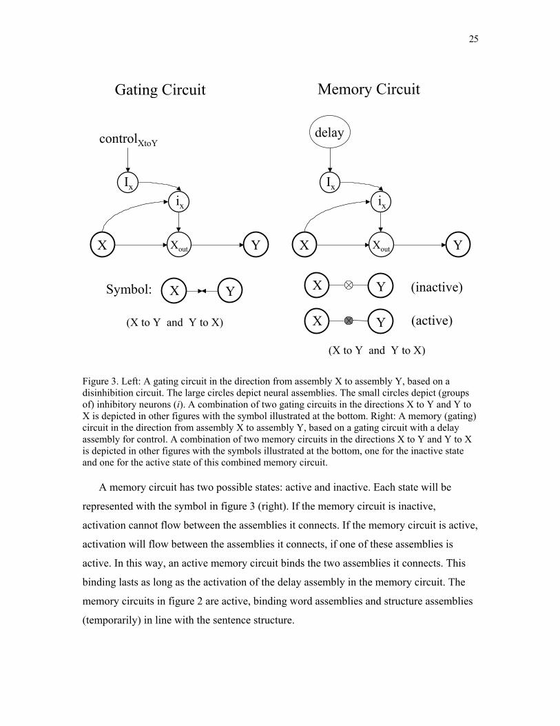
A gating circuit consists of a disinhibition circuit (e.g., Gonchar and Burkhalter 1999).
Figure 3 (left) illustrates a gating circuit in the direction from assembly X to assembly Y.
The circuit controls the flow of activation by means of an external control signal. If X is
active, it activates an inhibition neuron ix, which inhibits the flow of activation from X to
Xout. When ix is inhibited by another inhibition neuron (Ix), activated by an external
control signal, X activates Xout, and Xout activates Y. A gating circuit from Y to X operates
in the same way. Control of activation can be direction specific. With a control signal in
the direction from X to Y, activation will flow in this direction (if X is active), but not in
the direction from Y to X. The symbol in figure 3 (left) will be used to represent the
combination of gating circuits in both directions (as in figure 2).
A memory circuit consists of a gating circuit in which the control signal results from
a ‘delay’ assembly. Figure 3 (right) illustrates a memory circuit in the direction of X to Y.
However, each memory circuit in the architecture consists of two such circuits in both
directions (X to Y and Y to X). The delay assembly (that controls the flow of activation in
both directions) is activated when X and Y are active simultaneously (see below), and it
remains active for a while (even when X and Y are no longer active), due to the
reverberating nature of the activation in this assembly.
25
Figure 3. Left: A gating circuit in the direction from assembly X to assembly Y, based on a disinhibition circuit. The large circles depict neural assemblies. The small circles depict (groups of) inhibitory neurons (i). A combination of two gating circuits in the directions X to Y and Y to X is depicted in other figures with the symbol illustrated at the bottom. Right: A memory (gating) circuit in the direction from assembly X to assembly Y, based on a gating circuit with a delay assembly for control. A combination of two memory circuits in the directions X to Y and Y to X is depicted in other figures with the symbols illustrated at the bottom, one for the inactive state and one for the active state of this combined memory circuit.
A memory circuit has two possible states: active and inactive. Each state will be
represented with the symbol in figure 3 (right). If the memory circuit is inactive,
activation cannot flow between the assemblies it connects. If the memory circuit is active,
activation will flow between the assemblies it connects, if one of these assemblies is
active. In this way, an active memory circuit binds the two assemblies it connects. This
binding lasts as long as the activation of the delay assembly in the memory circuit. The
memory circuits in figure 2 are active, binding word assemblies and structure assemblies
(temporarily) in line with the sentence structure.
Xout YX
ix
Ix
controlXtoY
Gating Circuit
Symbol: X Y
(X to Y and Y to X)
Xout YX
ix
Ix
(X to Y and Y to X)
Memory Circuit
delay
X Y
X Y
(active)
(inactive)
26
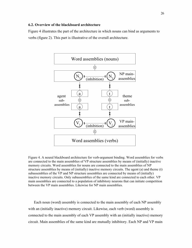
6.2. Overview of the blackboard architecture
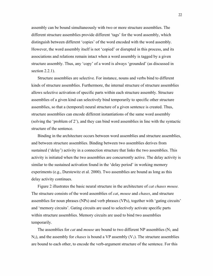
Figure 4 illustrates the part of the architecture in which nouns can bind as arguments to
verbs (figure 2). This part is illustrative of the overall architecture.
Figure 4. A neural blackboard architecture for verb-argument binding. Word assemblies for verbs are connected to the main assemblies of VP structure assemblies by means of (initially) inactive memory circuits. Word assemblies for nouns are connected to the main assemblies of NP structure assemblies by means of (initially) inactive memory circuits. The agent (a) and theme (t) subassemblies of the VP and NP structure assemblies are connected by means of (initially) inactive memory circuits. Only subassemblies of the same kind are connected to each other. VP main assemblies are connected to a population of inhibitory neurons that can initiate competition between the VP main assemblies. Likewise for NP main assemblies.
Each noun (word) assembly is connected to the main assembly of each NP assembly
with an (initially inactive) memory circuit. Likewise, each verb (word) assembly is
connected to the main assembly of each VP assembly with an (initially inactive) memory
circuit. Main assemblies of the same kind are mutually inhibitory. Each NP and VP main
VjVi
Word assemblies (verbs)
a
a
Word assemblies (nouns)
t
t
Nx Ny
VP main-assemblies
agentsub-
assemblies
themesub-
assemblies
NP main-assemblies
(inhibition)
(inhibition)
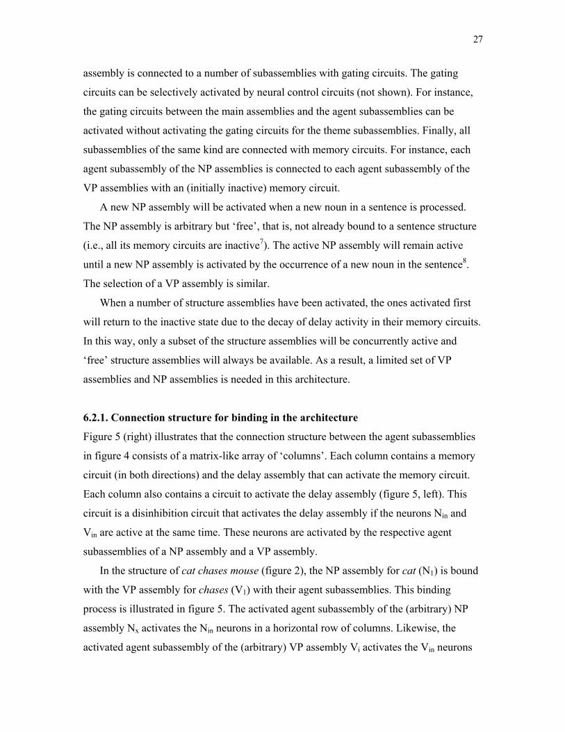
27
assembly is connected to a number of subassemblies with gating circuits. The gating
circuits can be selectively activated by neural control circuits (not shown). For instance,
the gating circuits between the main assemblies and the agent subassemblies can be
activated without activating the gating circuits for the theme subassemblies. Finally, all
subassemblies of the same kind are connected with memory circuits. For instance, each
agent subassembly of the NP assemblies is connected to each agent subassembly of the
VP assemblies with an (initially inactive) memory circuit.
A new NP assembly will be activated when a new noun in a sentence is processed.
The NP assembly is arbitrary but ‘free’, that is, not already bound to a sentence structure
(i.e., all its memory circuits are inactive7). The active NP assembly will remain active
until a new NP assembly is activated by the occurrence of a new noun in the sentence8.
The selection of a VP assembly is similar.
When a number of structure assemblies have been activated, the ones activated first
will return to the inactive state due to the decay of delay activity in their memory circuits.
In this way, only a subset of the structure assemblies will be concurrently active and
‘free’ structure assemblies will always be available. As a result, a limited set of VP
assemblies and NP assemblies is needed in this architecture.
6.2.1. Connection structure for binding in the architecture
Figure 5 (right) illustrates that the connection structure between the agent subassemblies
in figure 4 consists of a matrix-like array of ‘columns’. Each column contains a memory
circuit (in both directions) and the delay assembly that can activate the memory circuit.
Each column also contains a circuit to activate the delay assembly (figure 5, left). This
circuit is a disinhibition circuit that activates the delay assembly if the neurons Nin and
Vin are active at the same time. These neurons are activated by the respective agent
subassemblies of a NP assembly and a VP assembly.
In the structure of cat chases mouse (figure 2), the NP assembly for cat (N1) is bound
with the VP assembly for chases (V1) with their agent subassemblies. This binding
process is illustrated in figure 5. The activated agent subassembly of the (arbitrary) NP
assembly Nx activates the Nin neurons in a horizontal row of columns. Likewise, the
activated agent subassembly of the (arbitrary) VP assembly Vi activates the Vin neurons
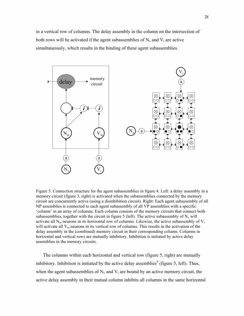
28
in a vertical row of columns. The delay assembly in the column on the intersection of
both rows will be activated if the agent subassemblies of Nx and Vi are active
simultaneously, which results in the binding of these agent subassemblies.
Figure 5. Connection structure for the agent subassemblies in figure 4. Left: a delay assembly in a memory circuit (figure 3, right) is activated when the subassemblies connected by the memory circuit are concurrently active (using a disinhibition circuit). Right: Each agent subassembly of all NP assemblies is connected to each agent subassembly of all VP assemblies with a specific ‘column’ in an array of columns. Each column consists of the memory circuits that connect both subassemblies, together with the circuit in figure 5 (left). The active subassembly of Nx will activate all Nin neurons in its horizontal row of columns. Likewise, the active subassembly of Vi will activate all Vin neurons in its vertical row of columns. This results in the activation of the delay assembly in the (combined) memory circuit in their corresponding column. Columns in horizontal and vertical rows are mutually inhibitory. Inhibition is initiated by active delay assemblies in the memory circuits.
The columns within each horizontal and vertical row (figure 5, right) are mutually
inhibitory. Inhibition is initiated by the active delay assemblies9 (figure 5, left). Thus,
when the agent subassemblies of Nx and Vi are bound by an active memory circuit, the
active delay assembly in their mutual column inhibits all columns in the same horizontal
Vi
a
Nx a
Nx
a
i i
delay
Vi
a
memory circuit
Nin Vin
29
and vertical row. This prevents a second binding of Nx with another VP assembly, or of
Vi with another NP assembly, with agent subassemblies.
The connection structure illustrated in figure 5 is illustrative of every connection
structure in the architecture in which assemblies are (temporarily) bound, including the
binding of V1 and N2 (figure 2) with their theme subassemblies.
In the binding process of the sentence in figure 2, the assembly for cat is bound to an
arbitrary (‘free’) NP assembly by the activated memory circuit that connects the two
assemblies. Likewise, the assembly for chases is bound to a VP assembly. The binding of
cat as the agent of chases results from activating the gating circuits between the NP and
VP main assemblies and their agent subassemblies. The active NP and VP main
assemblies (N1 for cat and V1 for chases) will then activate their agent subassemblies,
which results in the binding of these two agent subassemblies (as illustrated in figure 5).
Gating circuits will be activated by neural control circuits. These circuits instantiate
syntactic (parsing) operations, based on the active word assemblies and the activation
state of the blackboard. In the case of cat chases mouse, these circuits will detect that in
cat chases (or N-V), cat is the agent of the verb chases. In response, they will activate the
gating circuits for the agent subassemblies of all NPs and VPs. The binding of mouse as
the theme of chases proceeds in a similar manner. We will present an example of a
control circuit later on.
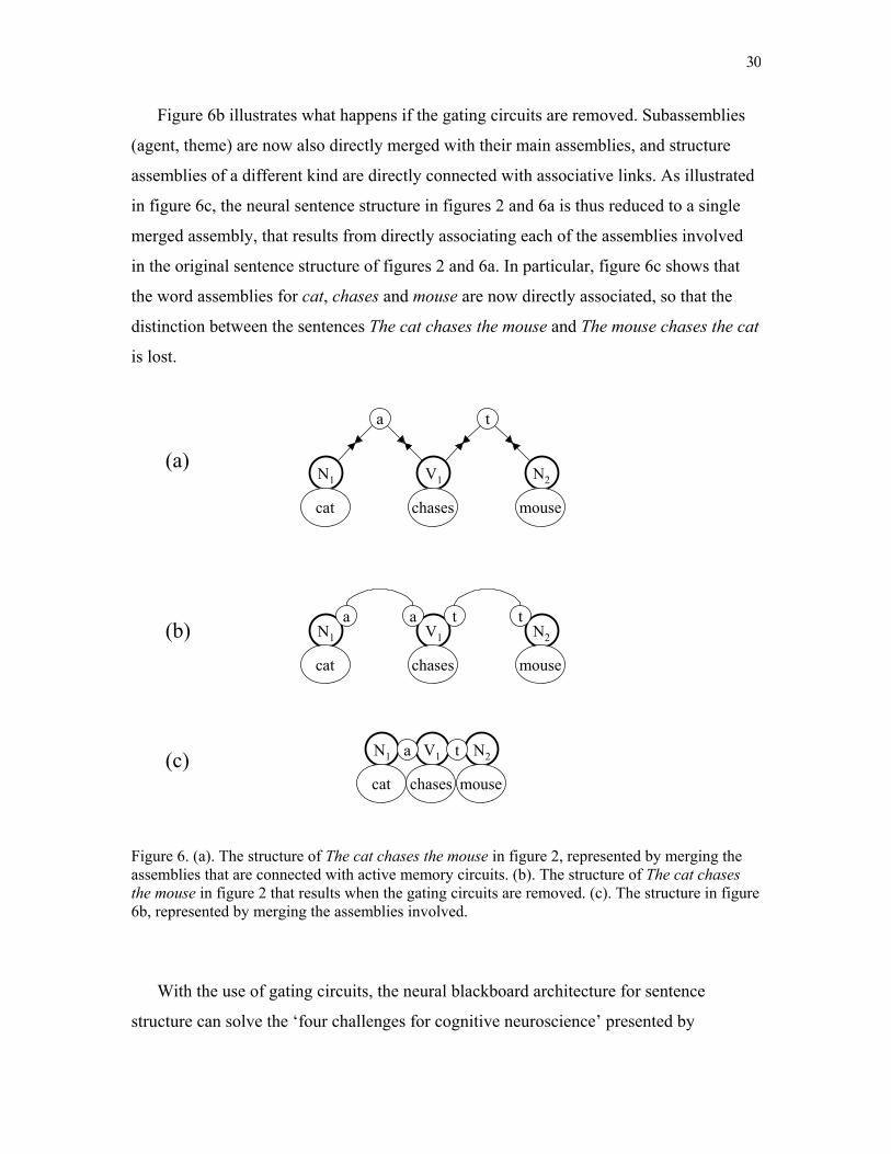
6.2.2. The effect of gating and memory circuits in the architecture
When a memory circuit is active, activation can flow between the two assemblies it
connects (figure 3, right). The two connected assemblies are then temporarily associated,
or ‘merged’, into a single assembly. Figure 6a illustrates the merging of assemblies for
the structure of The cat chases the mouse (figure 2). In figure 6a, the word assemblies are
directly connected (merged) with the main assemblies of their structure assemblies.
Likewise, the agent subassemblies and theme subassemblies are merged into single
assemblies (one for agent, and one for theme). The resulting structure shows that the
backbone of a neural sentence structure in this architecture is given by the gating circuits.
30
Figure 6b illustrates what happens if the gating circuits are removed. Subassemblies
(agent, theme) are now also directly merged with their main assemblies, and structure
assemblies of a different kind are directly connected with associative links. As illustrated
in figure 6c, the neural sentence structure in figures 2 and 6a is thus reduced to a single
merged assembly, that results from directly associating each of the assemblies involved
in the original sentence structure of figures 2 and 6a. In particular, figure 6c shows that
the word assemblies for cat, chases and mouse are now directly associated, so that the
distinction between the sentences The cat chases the mouse and The mouse chases the cat
is lost.
Figure 6. (a). The structure of The cat chases the mouse in figure 2, represented by merging the assemblies that are connected with active memory circuits. (b). The structure of The cat chases the mouse in figure 2 that results when the gating circuits are removed. (c). The structure in figure 6b, represented by merging the assemblies involved.
With the use of gating circuits, the neural blackboard architecture for sentence
structure can solve the ‘four challenges for cognitive neuroscience’ presented by
N1
cat
V1
a
N2
t
mousechases
N1
cat
V1a N2t
mousechases
N1
cat
V1
aN2
t
mousechases
a t
(a)
(b)
(c)

31
Jackendoff (2002, see section 2), as discussed below.
6.3. Multiple instantiation and binding in the architecture
Figure 7 (left, right) illustrates the neural structures of the sentences The cat chases the
mouse, The mouse chases the cat and The cat bites the dog in the neural blackboard
architecture (in the manner of figure 6a). The words cat, mouse and chases occur in more
than one sentence, which creates the problem of multiple instantiation (the problem of 2)
for their word assemblies.
Figure 7. Left: combined instantiation of the sentences cat chases mouse, mouse chases cat and cat bites dog in the architecture illustrated in figure 4. The multiple instantiations of cat, chases, and mouse in different sentences (and in different thematic roles) are distinguished by the different NP or VP structure assemblies to which they are bound. Right: the activation of the word assembly for cat and the word assembly for chases, due to the question “Whom does the cat chase?”
Figure 7 shows that this problem is solved by the use of structure assemblies. For
instance, the word assembly for cat is bound to the NP assemblies N1, N4 and N5.
N3
mouse
V2
a
N4
t
catchases
N1
cat
V1
a
N2
t
mousechases
N5
cat
V3
a
N6
t
dogbites
N3
mouse
V2
a
N4
t
catchases
N1
cat
V1
a
N2
t
mousechases
N5
cat
V3
a
N6
t
dogbites
32
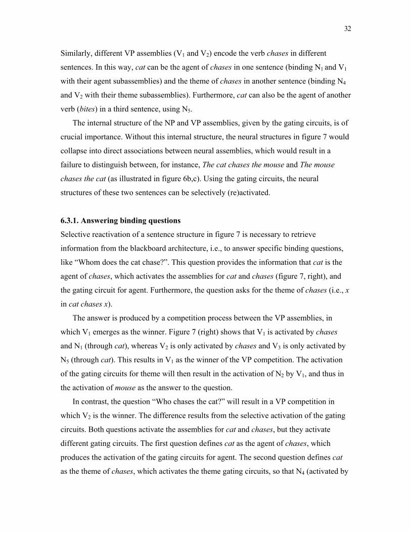
Similarly, different VP assemblies (V1 and V2) encode the verb chases in different
sentences. In this way, cat can be the agent of chases in one sentence (binding N1 and V1
with their agent subassemblies) and the theme of chases in another sentence (binding N4
and V2 with their theme subassemblies). Furthermore, cat can also be the agent of another
verb (bites) in a third sentence, using N5.
The internal structure of the NP and VP assemblies, given by the gating circuits, is of
crucial importance. Without this internal structure, the neural structures in figure 7 would
collapse into direct associations between neural assemblies, which would result in a
failure to distinguish between, for instance, The cat chases the mouse and The mouse
chases the cat (as illustrated in figure 6b,c). Using the gating circuits, the neural
structures of these two sentences can be selectively (re)activated.
6.3.1. Answering binding questions
Selective reactivation of a sentence structure in figure 7 is necessary to retrieve
information from the blackboard architecture, i.e., to answer specific binding questions,
like “Whom does the cat chase?”. This question provides the information that cat is the
agent of chases, which activates the assemblies for cat and chases (figure 7, right), and
the gating circuit for agent. Furthermore, the question asks for the theme of chases (i.e., x
in cat chases x).
The answer is produced by a competition process between the VP assemblies, in
which V1 emerges as the winner. Figure 7 (right) shows that V1 is activated by chases
and N1 (through cat), whereas V2 is only activated by chases and V3 is only activated by
N5 (through cat). This results in V1 as the winner of the VP competition. The activation
of the gating circuits for theme will then result in the activation of N2 by V1, and thus in
the activation of mouse as the answer to the question.
In contrast, the question “Who chases the cat?” will result in a VP competition in
which V2 is the winner. The difference results from the selective activation of the gating
circuits. Both questions activate the assemblies for cat and chases, but they activate
different gating circuits. The first question defines cat as the agent of chases, which
produces the activation of the gating circuits for agent. The second question defines cat
as the theme of chases, which activates the theme gating circuits, so that N4 (activated by
33
cat) can activate V2. This route of activation was blocked in case of the first question.
With the second question, V2 emerges as the winner because it receives the most
activation. Then, mouse can be produced as the answer, because the question asks for the
agent of chases (i.e., x in x chases cat).
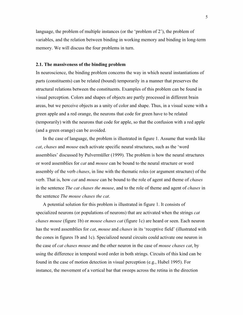
6.3.2. Simulation of the blackboard architecture
We have simulated the answer of “Whom does the cat chase?” with the sentences in
figure 7 stored simultaneously in the architecture. The simulation was based on the
dynamics of spiking neuron populations (i.e., average neuron activity). In all, 624
interconnected populations were simulated, representing the word assemblies, main
assemblies, subassemblies, gating circuits and memory circuits used to encode the
sentences in figure 7. The 624 populations evolved simultaneously during the simulation.
Appendix A1 provides further details of the simulation.
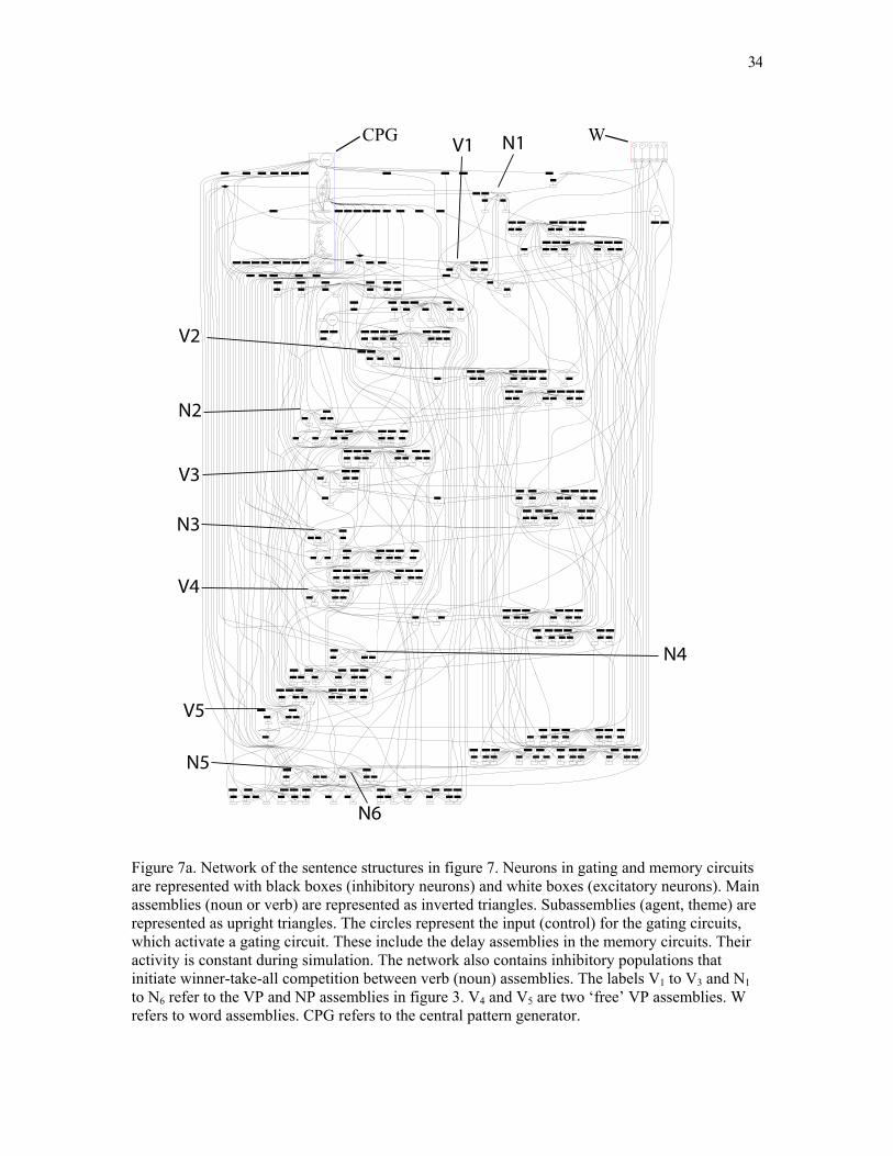
An overview of the network as simulated is presented in figure 7a. We used a visual
tool (dot by Koutsofious and North, 1996) to represent the network. The program dot
aims to place nodes (neurons) at a reasonable distance from each other and to minimize
the number of edge (connection) crossings. The network presented in figure 7a is the
same as the network presented in figure 7 (i.e., the three sentence structures). Both
networks can be converted into each other by successively inserting the structures
presented in figures 3, 4, and 5 in the structures presented in figure 7.
34
Figure 7a. Network of the sentence structures in figure 7. Neurons in gating and memory circuits are represented with black boxes (inhibitory neurons) and white boxes (excitatory neurons). Main assemblies (noun or verb) are represented as inverted triangles. Subassemblies (agent, theme) are represented as upright triangles. The circles represent the input (control) for the gating circuits, which activate a gating circuit. These include the delay assemblies in the memory circuits. Their activity is constant during simulation. The network also contains inhibitory populations that initiate winner-take-all competition between verb (noun) assemblies. The labels V1 to V3 and N1 to N6 refer to the VP and NP assemblies in figure 3. V4 and V5 are two ‘free’ VP assemblies. W refers to word assemblies. CPG refers to the central pattern generator.
John
john_exc
Bill
bill_exc
Mary
mary_exc
loves
love_exc
sees
sees_exc
LimAssemblyinput_1
LimAssemblyinput_4
LimAssemblyinput_5
LimAssemblyinput_2
LimAssemblyinput_3
LimAssemblyinput_7
LimAssemblyinput_8
LimAssemblyinput_9
LimAssemblyinput_10
LimAssemblyinput_11
I_center1
LimAssemblyhub_1
LimAssemblyhub_2
LimAssemblyhub_3
LimAssemblyhub_4
LimAssemblyhub_5 LimAssemblyhub_6
Gate_e1_1
Gate_i1_1
Gate_e1_2
Gate_i1_2
Gate_e2_3
Gate_i2_3
LimAssemblyagent_1
Gate_e2_1
Gate_i2_1
Gate_e1_34
Gate_i1_34
Gate_e1_35
Gate_i1_35
Gate_e1_36
Gate_i1_36
Gate_e1_37
Gate_i1_37
Gate_e1_38
Gate_i1_38
LimAssemblytheme_1
Gate_e2_2
Gate_i2_2
Gate_e2_64
Gate_i2_64
Gate_e2_70
Gate_i2_70
Gate_e2_76
Gate_i2_76
Gate_e2_82
Gate_i2_82
Gate_e2_88
Gate_i2_88
Gate_e1_3
Gate_i1_3
Gate_ifwd_1
Gate_ibwd_1
Gate_ifwd_2
Gate_ibwd_2
Gate_ifwd_3
Gate_ibwd_3
Gate_e1_4
Gate_i1_4
Gate_e1_5
Gate_i1_5
Gate_e2_6
Gate_i2_6
LimAssemblyagent_2
Gate_e2_4
Gate_i2_4
Gate_e1_39
Gate_i1_39
Gate_e1_40
Gate_i1_40
Gate_e1_41
Gate_i1_41
Gate_e1_42
Gate_i1_42
Gate_e1_43
Gate_i1_43
LimAssemblytheme_2
Gate_e2_5
Gate_i2_5
Gate_e2_65
Gate_i2_65
Gate_e2_71
Gate_i2_71
Gate_e2_77
Gate_i2_77
Gate_e2_83
Gate_i2_83
Gate_e2_89
Gate_i2_89
Gate_e1_6
Gate_i1_6
Gate_ifwd_4
Gate_ibwd_4
Gate_ifwd_5
Gate_ibwd_5
Gate_ifwd_6
Gate_ibwd_6
Gate_e1_7
Gate_i1_7
Gate_e1_8
Gate_i1_8
Gate_e2_9
Gate_i2_9
LimAssemblyagent_3
Gate_e2_7
Gate_i2_7
Gate_e1_44
Gate_i1_44
Gate_e1_45
Gate_i1_45
Gate_e1_46
Gate_i1_46
Gate_e1_47
Gate_i1_47
Gate_e1_48
Gate_i1_48
LimAssemblytheme_3
Gate_e2_8
Gate_i2_8
Gate_e2_66
Gate_i2_66
Gate_e2_72
Gate_i2_72
Gate_e2_78
Gate_i2_78
Gate_e2_84
Gate_i2_84
Gate_e2_90
Gate_i2_90
Gate_e1_9
Gate_i1_9
Gate_ifwd_7
Gate_ibwd_7
Gate_ifwd_8
Gate_ibwd_8
Gate_ifwd_9
Gate_ibwd_9
Gate_e1_10
Gate_i1_10
Gate_e1_11
Gate_i1_11
Gate_e2_12
Gate_i2_12
LimAssemblyagent_4
Gate_e2_10
Gate_i2_10
Gate_e1_49
Gate_i1_49
Gate_e1_50
Gate_i1_50
Gate_e1_51
Gate_i1_51
Gate_e1_52
Gate_i1_52
Gate_e1_53
Gate_i1_53
LimAssemblytheme_4
Gate_e2_11
Gate_i2_11
Gate_e2_67
Gate_i2_67
Gate_e2_73
Gate_i2_73
Gate_e2_79
Gate_i2_79
Gate_e2_85
Gate_i2_85
Gate_e2_91
Gate_i2_91
Gate_e1_12
Gate_i1_12
Gate_ifwd_10
Gate_ibwd_10
Gate_ifwd_11
Gate_ibwd_11
Gate_ifwd_12
Gate_ibwd_12
Gate_e1_13
Gate_i1_13
Gate_e1_14
Gate_i1_14
Gate_e2_15
Gate_i2_15
LimAssemblyagent_5
Gate_e2_13
Gate_i2_13
Gate_e1_54
Gate_i1_54
Gate_e1_55
Gate_i1_55
Gate_e1_56
Gate_i1_56
Gate_e1_57
Gate_i1_57
Gate_e1_58
Gate_i1_58
LimAssemblytheme_5
Gate_e2_14
Gate_i2_14
Gate_e2_68
Gate_i2_68
Gate_e2_74
Gate_i2_74
Gate_e2_80
Gate_i2_80
Gate_e2_86
Gate_i2_86
Gate_e2_92
Gate_i2_92
Gate_e1_15
Gate_i1_15
Gate_ifwd_13
Gate_ibwd_13
Gate_ifwd_14
Gate_ibwd_14
Gate_ifwd_15
Gate_ibwd_15
Gate_e1_16
Gate_i1_16
Gate_e1_17
Gate_i1_17
Gate_e2_18
Gate_i2_18
LimAssemblyagent_6
Gate_e2_16
Gate_i2_16
Gate_e1_59
Gate_i1_59
Gate_e1_60
Gate_i1_60
Gate_e1_61
Gate_i1_61
Gate_e1_62
Gate_i1_62
Gate_e1_63
Gate_i1_63
LimAssemblytheme_6
Gate_e2_17
Gate_i2_17
Gate_e2_69
Gate_i2_69
Gate_e2_75
Gate_i2_75
Gate_e2_81
Gate_i2_81
Gate_e2_87
Gate_i2_87
Gate_e2_93
Gate_i2_93
LimAssemblyinput_6
Gate_e1_18
Gate_i1_18
Gate_ifwd_16
Gate_ibwd_16
Gate_ifwd_17
Gate_ibwd_17
Gate_ifwd_18
Gate_ibwd_18
I_center2
LimAssemblyhub_7
LimAssemblyhub_8
LimAssemblyhub_9
LimAssemblyhub_10
LimAssemblyhub_11
Gate_e1_19
Gate_i1_19
Gate_e1_20
Gate_i1_20
Gate_e2_21
Gate_i2_21
LimAssemblyagent_7
Gate_e2_19
Gate_i2_19
Gate_e2_34
Gate_i2_34
Gate_e2_39
Gate_i2_39
Gate_e2_44
Gate_i2_44
Gate_e2_49
Gate_i2_49
Gate_e2_54
Gate_i2_54
Gate_e2_59
Gate_i2_59
LimAssemblytheme_7
Gate_e2_20
Gate_i2_20
Gate_e1_64
Gate_i1_64
Gate_e1_65
Gate_i1_65
Gate_e1_66
Gate_i1_66
Gate_e1_67
Gate_i1_67
Gate_e1_68
Gate_i1_68
Gate_e1_69
Gate_i1_69
Gate_e1_21
Gate_i1_21
Gate_ifwd_19
Gate_ibwd_19
Gate_ifwd_20
Gate_ibwd_20
Gate_ifwd_21
Gate_ibwd_21
Gate_e1_22
Gate_i1_22
Gate_e1_23
Gate_i1_23
Gate_e2_24
Gate_i2_24
LimAssemblyagent_8
Gate_e2_22
Gate_i2_22
Gate_e2_35
Gate_i2_35
Gate_e2_40
Gate_i2_40
Gate_e2_45
Gate_i2_45
Gate_e2_50
Gate_i2_50
Gate_e2_55
Gate_i2_55
Gate_e2_60
Gate_i2_60
LimAssemblytheme_8
Gate_e2_23
Gate_i2_23
Gate_e1_70
Gate_i1_70
Gate_e1_71
Gate_i1_71
Gate_e1_72
Gate_i1_72
Gate_e1_73
Gate_i1_73
Gate_e1_74
Gate_i1_74
Gate_e1_75
Gate_i1_75
Gate_e1_24
Gate_i1_24
Gate_ifwd_22
Gate_ibwd_22
Gate_ifwd_23
Gate_ibwd_23
Gate_ifwd_24
Gate_ibwd_24
Gate_e1_25
Gate_i1_25
Gate_e1_26
Gate_i1_26
Gate_e2_27
Gate_i2_27
LimAssemblyagent_9
Gate_e2_25
Gate_i2_25
Gate_e2_36
Gate_i2_36
Gate_e2_41
Gate_i2_41
Gate_e2_46
Gate_i2_46
Gate_e2_51
Gate_i2_51
Gate_e2_56
Gate_i2_56
Gate_e2_61
Gate_i2_61
LimAssemblytheme_9
Gate_e2_26
Gate_i2_26
Gate_e1_76
Gate_i1_76
Gate_e1_77
Gate_i1_77
Gate_e1_78
Gate_i1_78
Gate_e1_79
Gate_i1_79
Gate_e1_80
Gate_i1_80
Gate_e1_81
Gate_i1_81
Gate_e1_27
Gate_i1_27
Gate_ifwd_25
Gate_ibwd_25
Gate_ifwd_26
Gate_ibwd_26
Gate_ifwd_27
Gate_ibwd_27
Gate_e1_28
Gate_i1_28
Gate_e1_29
Gate_i1_29
Gate_e2_30
Gate_i2_30
LimAssemblyagent_10
Gate_e2_28
Gate_i2_28
Gate_e2_37
Gate_i2_37
Gate_e2_42
Gate_i2_42
Gate_e2_47
Gate_i2_47
Gate_e2_52
Gate_i2_52
Gate_e2_57
Gate_i2_57
Gate_e2_62
Gate_i2_62
LimAssemblytheme_10
Gate_e2_29
Gate_i2_29
Gate_e1_82
Gate_i1_82
Gate_e1_83
Gate_i1_83
Gate_e1_84
Gate_i1_84
Gate_e1_85
Gate_i1_85
Gate_e1_86
Gate_i1_86
Gate_e1_87
Gate_i1_87
Gate_e1_30
Gate_i1_30
Gate_ifwd_28
Gate_ibwd_28
Gate_ifwd_29
Gate_ibwd_29
Gate_ifwd_30
Gate_ibwd_30
Gate_e1_31
Gate_i1_31
Gate_e1_32
Gate_i1_32
Gate_e2_33
Gate_i2_33
LimAssemblyagent_11
Gate_e2_31
Gate_i2_31
Gate_e2_38
Gate_i2_38
Gate_e2_43
Gate_i2_43
Gate_e2_48
Gate_i2_48
Gate_e2_53
Gate_i2_53
Gate_e2_58
Gate_i2_58
Gate_e2_63
Gate_i2_63
LimAssemblytheme_11
Gate_e2_32
Gate_i2_32
Gate_e1_88
Gate_i1_88
Gate_e1_89
Gate_i1_89
Gate_e1_90
Gate_i1_90
Gate_e1_91
Gate_i1_91
Gate_e1_92
Gate_i1_92
Gate_e1_93
Gate_i1_93
Gate_e1_33
Gate_i1_33
Gate_ifwd_31
Gate_ibwd_31
Gate_ifwd_32
Gate_ibwd_32
Gate_ifwd_33
Gate_ibwd_33
tonic_stimulation
tonic_1
tonic_2
agent_control
verb_competition_control
tonic_3
tonic_4
tonic_5
tonic_6
tonic_7noun_competition_control
tonic_8
tonic_9
theme_control
tonic_10
tonic_11
tonic_12tonic_14
tonic_13 tonic_15
noun_reversal_control
control_input
postfunction
Gate_ifwd_34
Gate_ibwd_34
Gate_ifwd_35
Gate_ibwd_35
Gate_ifwd_36
Gate_ibwd_36
Gate_ifwd_37
Gate_ibwd_37
Gate_ifwd_38
Gate_ibwd_38
Gate_ifwd_39
Gate_ibwd_39
Gate_ifwd_40
Gate_ibwd_40
Gate_ifwd_41
Gate_ibwd_41
Gate_ifwd_42
Gate_ibwd_42
Gate_ifwd_43
Gate_ibwd_43
Gate_ifwd_44
Gate_ibwd_44
Gate_ifwd_45
Gate_ibwd_45
Gate_ifwd_46
Gate_ibwd_46
Gate_ifwd_47
Gate_ibwd_47
Gate_ifwd_48
Gate_ibwd_48
Gate_ifwd_49
Gate_ibwd_49
Gate_ifwd_50
Gate_ibwd_50
Gate_ifwd_51
Gate_ibwd_51
Gate_ifwd_52
Gate_ibwd_52
Gate_ifwd_53
Gate_ibwd_53
Gate_ifwd_54
Gate_ibwd_54
Gate_ifwd_55
Gate_ibwd_55
Gate_ifwd_56
Gate_ibwd_56
Gate_ifwd_57
Gate_ibwd_57
Gate_ifwd_58
Gate_ibwd_58
Gate_ifwd_59
Gate_ibwd_59
Gate_ifwd_60
Gate_ibwd_60
Gate_ifwd_61
Gate_ibwd_61
Gate_ifwd_62
Gate_ibwd_62
Gate_ifwd_63
Gate_ibwd_63
Delay_agent
Gate_ifwd_64
Gate_ibwd_64
Gate_ifwd_65
Gate_ibwd_65
Gate_ifwd_66
Gate_ibwd_66
Gate_ifwd_67
Gate_ibwd_67
Gate_ifwd_68
Gate_ibwd_68
Gate_ifwd_69
Gate_ibwd_69
Gate_ifwd_70
Gate_ibwd_70
Gate_ifwd_71
Gate_ibwd_71
Gate_ifwd_72
Gate_ibwd_72
Gate_ifwd_73
Gate_ibwd_73
Gate_ifwd_74
Gate_ibwd_74
Gate_ifwd_75
Gate_ibwd_75
Gate_ifwd_76
Gate_ibwd_76
Gate_ifwd_77
Gate_ibwd_77
Gate_ifwd_78
Gate_ibwd_78
Gate_ifwd_79
Gate_ibwd_79
Gate_ifwd_80
Gate_ibwd_80
Gate_ifwd_81
Gate_ibwd_81
Gate_ifwd_82
Gate_ibwd_82
Gate_ifwd_83
Gate_ibwd_83
Gate_ifwd_84
Gate_ibwd_84
Gate_ifwd_85
Gate_ibwd_85
Gate_ifwd_86
Gate_ibwd_86
Gate_ifwd_87
Gate_ibwd_87
Gate_ifwd_88
Gate_ibwd_88
Gate_ifwd_89
Gate_ibwd_89
Gate_ifwd_90
Gate_ibwd_90
Gate_ifwd_91
Gate_ibwd_91
Gate_ifwd_92
Gate_ibwd_92
Gate_ifwd_93
Gate_ibwd_93
Delay_target
N1
N2
V3
N3
V4
N5
V5
N6
N4
V2
V1WCPG
35
Figure 8 (left, middle) illustrates the simulation of the network with activation of the
VP and NP assemblies labeled in figure 7a. The figure (middle) also shows two ‘free’ VP
main assemblies (V4, V5), not used in the sentence encoding of figure 7, to illustrate the
activation of free assemblies in this process. The simulation starts at t = 0 ms. Before that
time, the only active assemblies are the delay assemblies in the memory circuits (as in
figure 2).
The question “Whom does the cat chase?” provides information that cat is the agent
of chases and it asks for the theme of the sentence cat chases x. The production of the
answer consists of the selective activation of the word assembly for mouse. Backtracking
(see figure 7), this requires the selective activation of the NP main assembly N2, the
theme subassemblies for N2 and V1, and the VP main assembly V1 (in reversed order).
This process proceeds in a sequence of steps. We used a central pattern generator
(CPG) to control the sequence. Basically, a CPG consists of a sequence of neurons, in
which a neuron is active for a while before activation is passed on to the next neuron in
the sequence. CPGs can be used in motion control (e.g., Kling and Szekély 1968). Forms
of sequential motion control could provide a basis for analogous functions in language as
well (e.g., Dominey 1997).We assume that a question of the type cat chases x? activates
a specific (type-related) CPG. That is, the same CPG will be initiated with any question
of the form noun verb x?. The CPG used consisted of 15 neurons, each one active for 25
ms. This provides 15 time steps of 25 ms. The CPG was activated at t=300 ms (indicated
with the asterisk in figure 8). It initiated the following sequence: activate VP competition
(step 1-5), activate agent gating circuits (step 1-4), inhibit word assemblies (step 5),
activate NP competition (step 6), activate theme gating circuits for VP assemblies (step 8-
11), and activate theme gating circuits for NP assemblies (step 13-15).
Figure 8 shows the activation of the assemblies for cat and chases (beginning at t = 0
ms). To produce the selective activation of the word assembly for mouse, other word
assemblies cannot be active at that moment. Therefore, word assemblies are inhibited
after a certain time (step 5). The activation of cat results in the activation of the NP main
assemblies N1, N4, and N5 (figure 8, left), and the activation of chases results in the
activation of the VP main assemblies V1 and V2 (figure 8, middle). As long as V1 and V2
are both active, the question “Whom does the cat chase?” cannot be answered. To
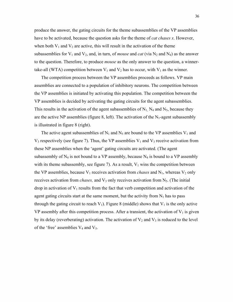
36
produce the answer, the gating circuits for the theme subassemblies of the VP assemblies
have to be activated, because the question asks for the theme of cat chases x. However,
when both V1 and V2 are active, this will result in the activation of the theme
subassemblies for V1 and V2, and, in turn, of mouse and cat (via N2 and N4) as the answer
to the question. Therefore, to produce mouse as the only answer to the question, a winner-
take-all (WTA) competition between V1 and V2 has to occur, with V1 as the winner.
The competition process between the VP assemblies proceeds as follows. VP main
assemblies are connected to a population of inhibitory neurons. The competition between
the VP assemblies is initiated by activating this population. The competition between the
VP assemblies is decided by activating the gating circuits for the agent subassemblies.
This results in the activation of the agent subassemblies of N1, N4 and N5, because they
are the active NP assemblies (figure 8, left). The activation of the N1-agent subassembly
is illustrated in figure 8 (right).
The active agent subassemblies of N1 and N5 are bound to the VP assemblies V1 and
V3 respectively (see figure 7). Thus, the VP assemblies V1 and V3 receive activation from
these NP assemblies when the ‘agent’ gating circuits are activated. (The agent
subassembly of N4 is not bound to a VP assembly, because N4 is bound to a VP assembly
with its theme subassembly, see figure 7). As a result, V1 wins the competition between
the VP assemblies, because V1 receives activation from chases and N1, whereas V2 only
receives activation from chases, and V3 only receives activation from N5. (The initial
drop in activation of V1 results from the fact that verb competition and activation of the
agent gating circuits start at the same moment, but the activity from N1 has to pass
through the gating circuit to reach V1). Figure 8 (middle) shows that V1 is the only active
VP assembly after this competition process. After a transient, the activation of V1 is given
by its delay (reverberating) activation. The activation of V2 and V3 is reduced to the level
of the ‘free’ assemblies V4 and V5.
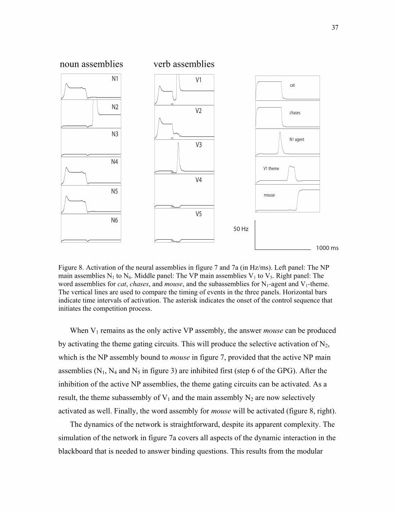
37
Figure 8. Activation of the neural assemblies in figure 7 and 7a (in Hz/ms). Left panel: The NP main assemblies N1 to N6. Middle panel: The VP main assemblies V1 to V5. Right panel: The word assemblies for cat, chases, and mouse, and the subassemblies for N1-agent and V1-theme. The vertical lines are used to compare the timing of events in the three panels. Horizontal bars indicate time intervals of activation. The asterisk indicates the onset of the control sequence that initiates the competition process.
When V1 remains as the only active VP assembly, the answer mouse can be produced
by activating the theme gating circuits. This will produce the selective activation of N2,
which is the NP assembly bound to mouse in figure 7, provided that the active NP main
assemblies (N1, N4 and N5 in figure 3) are inhibited first (step 6 of the GPG). After the
inhibition of the active NP assemblies, the theme gating circuits can be activated. As a
result, the theme subassembly of V1 and the main assembly N2 are now selectively
activated as well. Finally, the word assembly for mouse will be activated (figure 8, right).
The dynamics of the network is straightforward, despite its apparent complexity. The
simulation of the network in figure 7a covers all aspects of the dynamic interaction in the
blackboard that is needed to answer binding questions. This results from the modular
noun assemblies verb assembliesN1
N2
N3
N4
N5
N6
V1
V2
V3
V4
V5
1000 ms
50 Hz
cat
chases
N1 agent
V1 theme
mouse
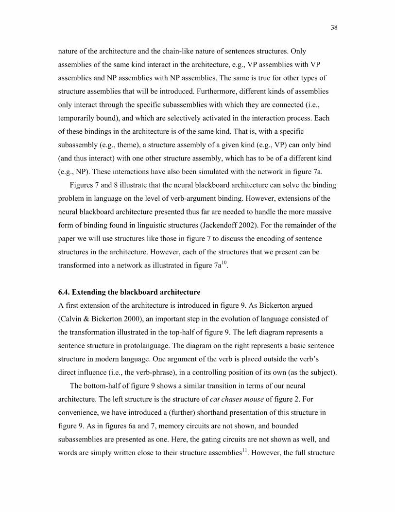
38
nature of the architecture and the chain-like nature of sentences structures. Only
assemblies of the same kind interact in the architecture, e.g., VP assemblies with VP
assemblies and NP assemblies with NP assemblies. The same is true for other types of
structure assemblies that will be introduced. Furthermore, different kinds of assemblies
only interact through the specific subassemblies with which they are connected (i.e.,
temporarily bound), and which are selectively activated in the interaction process. Each
of these bindings in the architecture is of the same kind. That is, with a specific
subassembly (e.g., theme), a structure assembly of a given kind (e.g., VP) can only bind
(and thus interact) with one other structure assembly, which has to be of a different kind
(e.g., NP). These interactions have also been simulated with the network in figure 7a.
Figures 7 and 8 illustrate that the neural blackboard architecture can solve the binding
problem in language on the level of verb-argument binding. However, extensions of the
neural blackboard architecture presented thus far are needed to handle the more massive
form of binding found in linguistic structures (Jackendoff 2002). For the remainder of the
paper we will use structures like those in figure 7 to discuss the encoding of sentence
structures in the architecture. However, each of the structures that we present can be
transformed into a network as illustrated in figure 7a10.
6.4. Extending the blackboard architecture
A first extension of the architecture is introduced in figure 9. As Bickerton argued
(Calvin & Bickerton 2000), an important step in the evolution of language consisted of
the transformation illustrated in the top-half of figure 9. The left diagram represents a
sentence structure in protolanguage. The diagram on the right represents a basic sentence
structure in modern language. One argument of the verb is placed outside the verb’s
direct influence (i.e., the verb-phrase), in a controlling position of its own (as the subject).
The bottom-half of figure 9 shows a similar transition in terms of our neural
architecture. The left structure is the structure of cat chases mouse of figure 2. For
convenience, we have introduced a (further) shorthand presentation of this structure in
figure 9. As in figures 6a and 7, memory circuits are not shown, and bounded
subassemblies are presented as one. Here, the gating circuits are not shown as well, and
words are simply written close to their structure assemblies11. However, the full structure
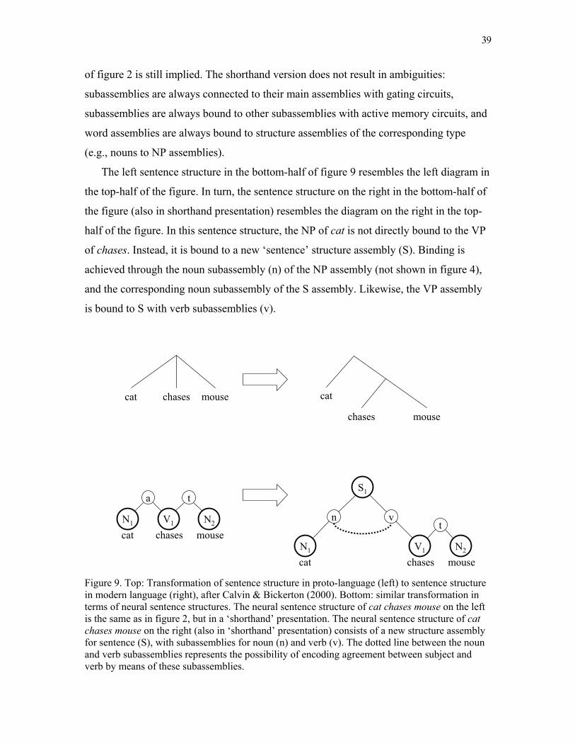
39
of figure 2 is still implied. The shorthand version does not result in ambiguities:
subassemblies are always connected to their main assemblies with gating circuits,
subassemblies are always bound to other subassemblies with active memory circuits, and
word assemblies are always bound to structure assemblies of the corresponding type
(e.g., nouns to NP assemblies).
The left sentence structure in the bottom-half of figure 9 resembles the left diagram in
the top-half of the figure. In turn, the sentence structure on the right in the bottom-half of
the figure (also in shorthand presentation) resembles the diagram on the right in the top-
half of the figure. In this sentence structure, the NP of cat is not directly bound to the VP
of chases. Instead, it is bound to a new ‘sentence’ structure assembly (S). Binding is
achieved through the noun subassembly (n) of the NP assembly (not shown in figure 4),
and the corresponding noun subassembly of the S assembly. Likewise, the VP assembly
is bound to S with verb subassemblies (v).
Figure 9. Top: Transformation of sentence structure in proto-language (left) to sentence structure in modern language (right), after Calvin & Bickerton (2000). Bottom: similar transformation in terms of neural sentence structures. The neural sentence structure of cat chases mouse on the left is the same as in figure 2, but in a ‘shorthand’ presentation. The neural sentence structure of cat chases mouse on the right (also in ‘shorthand’ presentation) consists of a new structure assembly for sentence (S), with subassemblies for noun (n) and verb (v). The dotted line between the noun and verb subassemblies represents the possibility of encoding agreement between subject and verb by means of these subassemblies.
cat mouse cat
mouse
chases
chases
N1
n
S1
V1
t
N2
v
cat chases mouse
V1
t
N2
a
chases mouseN1
cat
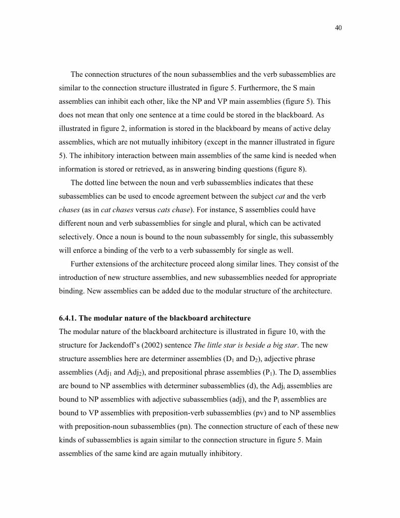
40
The connection structures of the noun subassemblies and the verb subassemblies are
similar to the connection structure illustrated in figure 5. Furthermore, the S main
assemblies can inhibit each other, like the NP and VP main assemblies (figure 5). This
does not mean that only one sentence at a time could be stored in the blackboard. As
illustrated in figure 2, information is stored in the blackboard by means of active delay
assemblies, which are not mutually inhibitory (except in the manner illustrated in figure
5). The inhibitory interaction between main assemblies of the same kind is needed when
information is stored or retrieved, as in answering binding questions (figure 8).
The dotted line between the noun and verb subassemblies indicates that these
subassemblies can be used to encode agreement between the subject cat and the verb
chases (as in cat chases versus cats chase). For instance, S assemblies could have
different noun and verb subassemblies for single and plural, which can be activated
selectively. Once a noun is bound to the noun subassembly for single, this subassembly
will enforce a binding of the verb to a verb subassembly for single as well.
Further extensions of the architecture proceed along similar lines. They consist of the
introduction of new structure assemblies, and new subassemblies needed for appropriate
binding. New assemblies can be added due to the modular structure of the architecture.
6.4.1. The modular nature of the blackboard architecture
The modular nature of the blackboard architecture is illustrated in figure 10, with the
structure for Jackendoff’s (2002) sentence The little star is beside a big star. The new
structure assemblies here are determiner assemblies (D1 and D2), adjective phrase
assemblies (Adj1 and Adj2), and prepositional phrase assemblies (P1). The Di assemblies
are bound to NP assemblies with determiner subassemblies (d), the Adji assemblies are
bound to NP assemblies with adjective subassemblies (adj), and the Pi assemblies are
bound to VP assemblies with preposition-verb subassemblies (pv) and to NP assemblies
with preposition-noun subassemblies (pn). The connection structure of each of these new
kinds of subassemblies is again similar to the connection structure in figure 5. Main
assemblies of the same kind are again mutually inhibitory.

41
Figure 10. Neural sentence structure for The little star is beside a big star. The structure assemblies are similar to those in figure 9 (bottom-right), with new structure assemblies for determiner (Di), adjective phrase (Adji) and prepositional phrase (Pi), and new subassemblies for determiner (d), adjective (adj), preposition-verb (pv) and preposition-noun (pn).
This sentence structure again illustrates the solution of the problem of 2 provided by
the architecture, and it illustrates the solution of the massiveness of the binding problem
in linguistic structures. The word assembly for star can participate in two different
constituents of the sentence, because it is bound to two different NP assemblies. Bound to
N1, star has the determiner the and the adjective little, and it constitutes the subject of the
sentence, bound directly to S. Bound to N2, star has the determine a and the adjective big,
and it is bound to the preposition beside, which is bound to the verb of the sentence.
Questions can be again be answered by selectively activating structure assemblies and
gating circuits. For instance, the question “Which star is beside a big star?” can be
answered if S1 is activated, together with the gating circuits for the noun subassemblies
(the question asks for the adjective of the subject). When N1 is activated, D1 and Adj1 can
also be activated, which produces the answer the little star. S1 will be activated due to the
information is beside a big star provided by the question. The phrase a big star activates
N2, which thus initially wins the competition over N1. However, after the selection of S1,
N1
n
S1
V1
d
N2
v
star is
pv
P1
pn
adj
Adj2
D1
little
adj
Adj1
the
d
star
D2
a big
beside
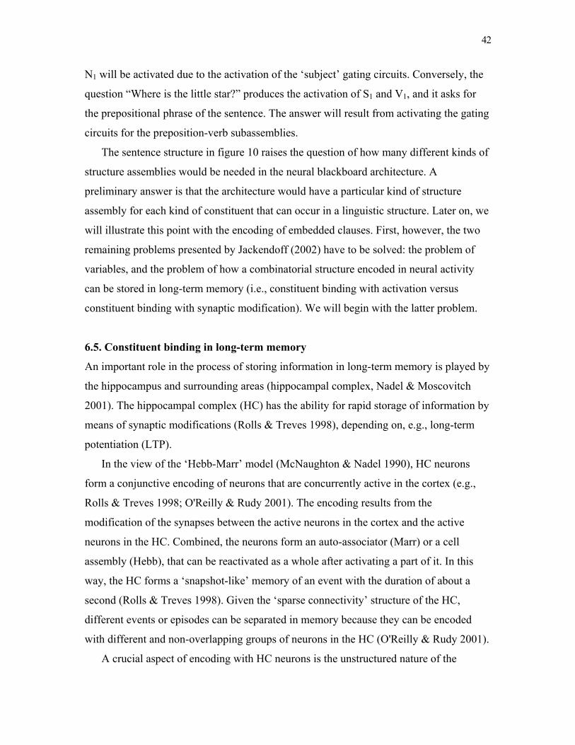
42
N1 will be activated due to the activation of the ‘subject’ gating circuits. Conversely, the
question “Where is the little star?” produces the activation of S1 and V1, and it asks for
the prepositional phrase of the sentence. The answer will result from activating the gating
circuits for the preposition-verb subassemblies.
The sentence structure in figure 10 raises the question of how many different kinds of
structure assemblies would be needed in the neural blackboard architecture. A
preliminary answer is that the architecture would have a particular kind of structure
assembly for each kind of constituent that can occur in a linguistic structure. Later on, we
will illustrate this point with the encoding of embedded clauses. First, however, the two
remaining problems presented by Jackendoff (2002) have to be solved: the problem of
variables, and the problem of how a combinatorial structure encoded in neural activity
can be stored in long-term memory (i.e., constituent binding with activation versus
constituent binding with synaptic modification). We will begin with the latter problem.
6.5. Constituent binding in long-term memory
An important role in the process of storing information in long-term memory is played by
the hippocampus and surrounding areas (hippocampal complex, Nadel & Moscovitch
2001). The hippocampal complex (HC) has the ability for rapid storage of information by
means of synaptic modifications (Rolls & Treves 1998), depending on, e.g., long-term
potentiation (LTP).
In the view of the ‘Hebb-Marr’ model (McNaughton & Nadel 1990), HC neurons
form a conjunctive encoding of neurons that are concurrently active in the cortex (e.g.,
Rolls & Treves 1998; O'Reilly & Rudy 2001). The encoding results from the
modification of the synapses between the active neurons in the cortex and the active
neurons in the HC. Combined, the neurons form an auto-associator (Marr) or a cell
assembly (Hebb), that can be reactivated as a whole after activating a part of it. In this
way, the HC forms a ‘snapshot-like’ memory of an event with the duration of about a
second (Rolls & Treves 1998). Given the ‘sparse connectivity’ structure of the HC,
different events or episodes can be separated in memory because they can be encoded
with different and non-overlapping groups of neurons in the HC (O'Reilly & Rudy 2001).
A crucial aspect of encoding with HC neurons is the unstructured nature of the
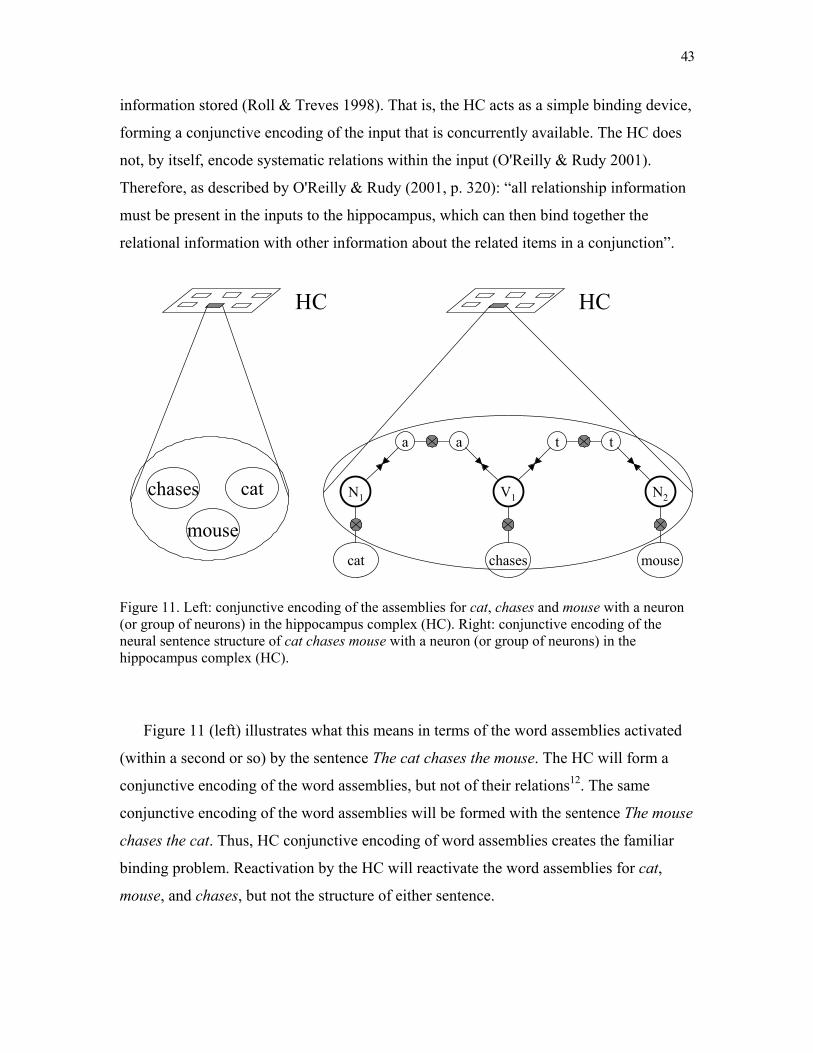
43
information stored (Roll & Treves 1998). That is, the HC acts as a simple binding device,
forming a conjunctive encoding of the input that is concurrently available. The HC does
not, by itself, encode systematic relations within the input (O'Reilly & Rudy 2001).
Therefore, as described by O'Reilly & Rudy (2001, p. 320): “all relationship information
must be present in the inputs to the hippocampus, which can then bind together the
relational information with other information about the related items in a conjunction”.
Figure 11. Left: conjunctive encoding of the assemblies for cat, chases and mouse with a neuron (or group of neurons) in the hippocampus complex (HC). Right: conjunctive encoding of the neural sentence structure of cat chases mouse with a neuron (or group of neurons) in the hippocampus complex (HC).
Figure 11 (left) illustrates what this means in terms of the word assemblies activated
(within a second or so) by the sentence The cat chases the mouse. The HC will form a
conjunctive encoding of the word assemblies, but not of their relations12. The same
conjunctive encoding of the word assemblies will be formed with the sentence The mouse
chases the cat. Thus, HC conjunctive encoding of word assemblies creates the familiar
binding problem. Reactivation by the HC will reactivate the word assemblies for cat,
mouse, and chases, but not the structure of either sentence.
HC
N1
cat
V1
a a
chases
N2
t t
mouse
HC
mouse
chases cat
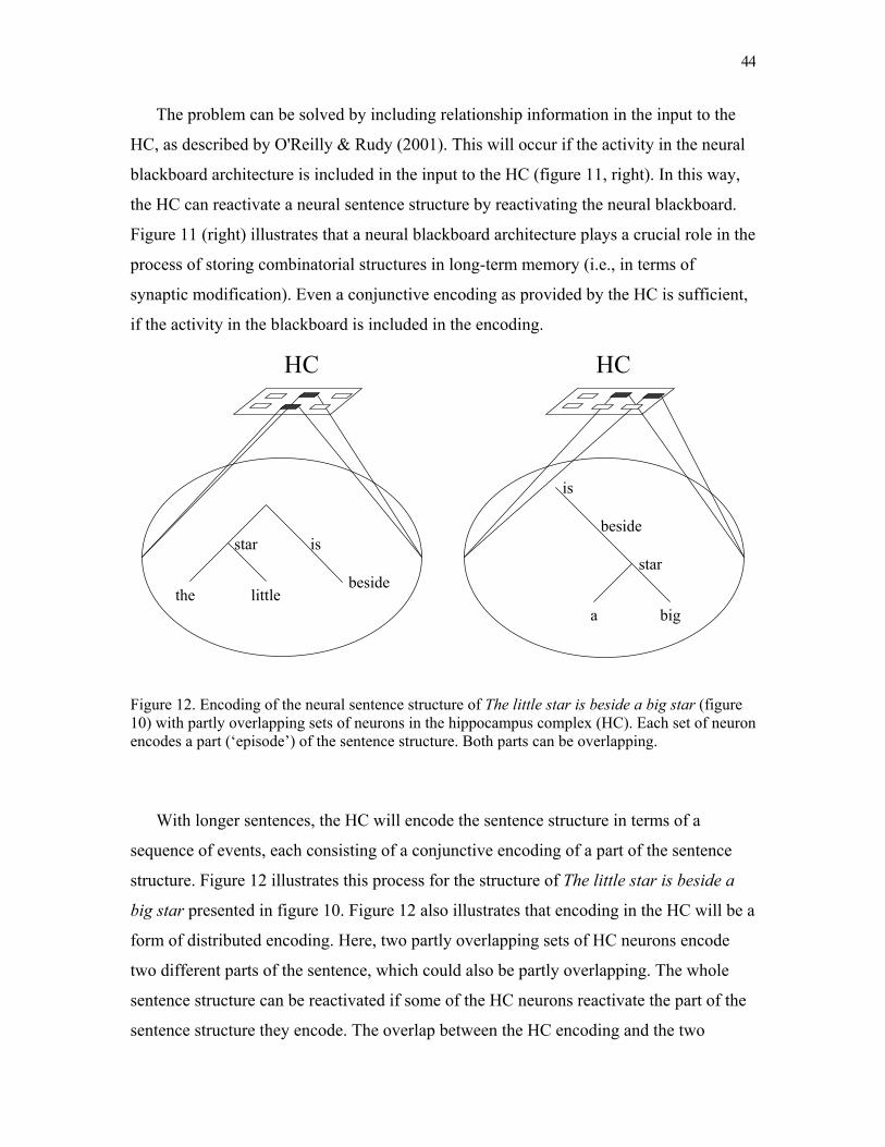
44
The problem can be solved by including relationship information in the input to the
HC, as described by O'Reilly & Rudy (2001). This will occur if the activity in the neural
blackboard architecture is included in the input to the HC (figure 11, right). In this way,
the HC can reactivate a neural sentence structure by reactivating the neural blackboard.
Figure 11 (right) illustrates that a neural blackboard architecture plays a crucial role in the
process of storing combinatorial structures in long-term memory (i.e., in terms of
synaptic modification). Even a conjunctive encoding as provided by the HC is sufficient,
if the activity in the blackboard is included in the encoding.
Figure 12. Encoding of the neural sentence structure of The little star is beside a big star (figure 10) with partly overlapping sets of neurons in the hippocampus complex (HC). Each set of neuron encodes a part (‘episode’) of the sentence structure. Both parts can be overlapping.
With longer sentences, the HC will encode the sentence structure in terms of a
sequence of events, each consisting of a conjunctive encoding of a part of the sentence
structure. Figure 12 illustrates this process for the structure of The little star is beside a
big star presented in figure 10. Figure 12 also illustrates that encoding in the HC will be a
form of distributed encoding. Here, two partly overlapping sets of HC neurons encode
two different parts of the sentence, which could also be partly overlapping. The whole
sentence structure can be reactivated if some of the HC neurons reactivate the part of the
sentence structure they encode. The overlap between the HC encoding and the two
HC HC
is
beside
star
a big
star is
the littlebeside

45
sentence structures can then result in the activation of the remaining part of the sentence
structure.
6.5.1. One-trial learning
In particular, the activity of the delay assemblies in the memory circuits has to be
included in the input to the HC, because the structure of a sentence is completely
determined by the set of active delay assemblies. In fact, as hinted at in figure 11 (right),
the HC encoding would not have to include all (or even any) of the word assemblies of
the sentence. The overall structure can be retrieved (i.e., binding questions can be
answered) as long as the delay assemblies can be reactivated by the HC.
The fact that HC encoding of the active delay assemblies is sufficient to store the
sentence structure in memory constitutes an important aspect of the use of delay activity
as a binding mechanism. The delay assemblies in the blackboard can remain active
concurrently without causing interference, unlike the word and structure assemblies. The
reverberating activity of delay assemblies will then provide sufficient time for the process
of synaptic modification to proceed (e.g., long-term potentiation takes in the order of 1-4
seconds, spoken sentences are processed in the order of 3 to 4 words per second).
In particular, this solves the problem of one-trial learning, as described by Jackendoff
(2002, p. 66): “It is usually argued that transient connections have the effect of gradually
adjusting synaptic weights (so-called Hebbian learning). But what about cases in which
one trial is sufficient for learning? For example, you say to me, I’ll meet you for lunch at
noon. I reply, OK, and indeed we do show up as agreed. My long-term memory has been
laid in on the basis of one trial; there hasn’t been any opportunity to adjust synaptic
weights gradually”.
Figure 11 (right) illustrates how one-trial learning can proceed by means of the
blackboard architecture. The word assemblies in The cat chases the mouse are indeed
activated briefly, to prevent the interference effects that would otherwise occur. But the
delay assemblies can remain active for a longer period, because they do not interfere with
each other. This provides the opportunity to adjust the synaptic weights between the HC
and the delay assemblies gradually, in line with Hebbian learning. In this way, a long-
term memory of a sentence structure can be formed on the basis of one trial.
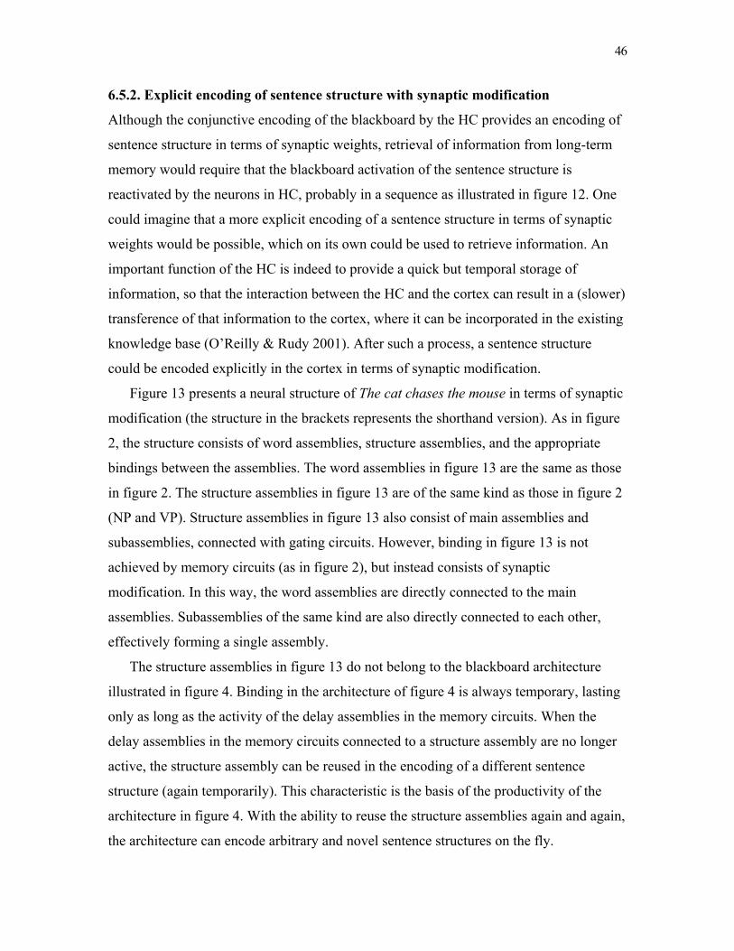
46
6.5.2. Explicit encoding of sentence structure with synaptic modification
Although the conjunctive encoding of the blackboard by the HC provides an encoding of
sentence structure in terms of synaptic weights, retrieval of information from long-term
memory would require that the blackboard activation of the sentence structure is
reactivated by the neurons in HC, probably in a sequence as illustrated in figure 12. One
could imagine that a more explicit encoding of a sentence structure in terms of synaptic
weights would be possible, which on its own could be used to retrieve information. An
important function of the HC is indeed to provide a quick but temporal storage of
information, so that the interaction between the HC and the cortex can result in a (slower)
transference of that information to the cortex, where it can be incorporated in the existing
knowledge base (O’Reilly & Rudy 2001). After such a process, a sentence structure
could be encoded explicitly in the cortex in terms of synaptic modification.
Figure 13 presents a neural structure of The cat chases the mouse in terms of synaptic
modification (the structure in the brackets represents the shorthand version). As in figure
2, the structure consists of word assemblies, structure assemblies, and the appropriate
bindings between the assemblies. The word assemblies in figure 13 are the same as those
in figure 2. The structure assemblies in figure 13 are of the same kind as those in figure 2
(NP and VP). Structure assemblies in figure 13 also consist of main assemblies and
subassemblies, connected with gating circuits. However, binding in figure 13 is not
achieved by memory circuits (as in figure 2), but instead consists of synaptic
modification. In this way, the word assemblies are directly connected to the main
assemblies. Subassemblies of the same kind are also directly connected to each other,
effectively forming a single assembly.
The structure assemblies in figure 13 do not belong to the blackboard architecture
illustrated in figure 4. Binding in the architecture of figure 4 is always temporary, lasting
only as long as the activity of the delay assemblies in the memory circuits. When the
delay assemblies in the memory circuits connected to a structure assembly are no longer
active, the structure assembly can be reused in the encoding of a different sentence
structure (again temporarily). This characteristic is the basis of the productivity of the
architecture in figure 4. With the ability to reuse the structure assemblies again and again,
the architecture can encode arbitrary and novel sentence structures on the fly.
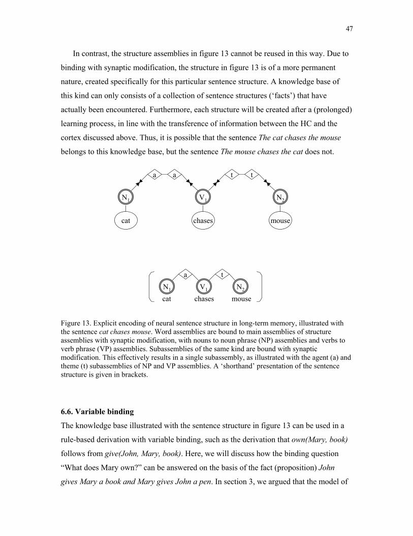
47
In contrast, the structure assemblies in figure 13 cannot be reused in this way. Due to
binding with synaptic modification, the structure in figure 13 is of a more permanent
nature, created specifically for this particular sentence structure. A knowledge base of
this kind can only consists of a collection of sentence structures (‘facts’) that have
actually been encountered. Furthermore, each structure will be created after a (prolonged)
learning process, in line with the transference of information between the HC and the
cortex discussed above. Thus, it is possible that the sentence The cat chases the mouse
belongs to this knowledge base, but the sentence The mouse chases the cat does not.
Figure 13. Explicit encoding of neural sentence structure in long-term memory, illustrated with the sentence cat chases mouse. Word assemblies are bound to main assemblies of structure assemblies with synaptic modification, with nouns to noun phrase (NP) assemblies and verbs to verb phrase (VP) assemblies. Subassemblies of the same kind are bound with synaptic modification. This effectively results in a single subassembly, as illustrated with the agent (a) and theme (t) subassemblies of NP and VP assemblies. A ‘shorthand’ presentation of the sentence structure is given in brackets.
6.6. Variable binding
The knowledge base illustrated with the sentence structure in figure 13 can be used in a
rule-based derivation with variable binding, such as the derivation that own(Mary, book)
follows from give(John, Mary, book). Here, we will discuss how the binding question
“What does Mary own?” can be answered on the basis of the fact (proposition) John
gives Mary a book and Mary gives John a pen. In section 3, we argued that the model of
a
N1
cat
V1
chases
N2
mouse
a t t
V1 N2
chases mouseN1
cat
a t
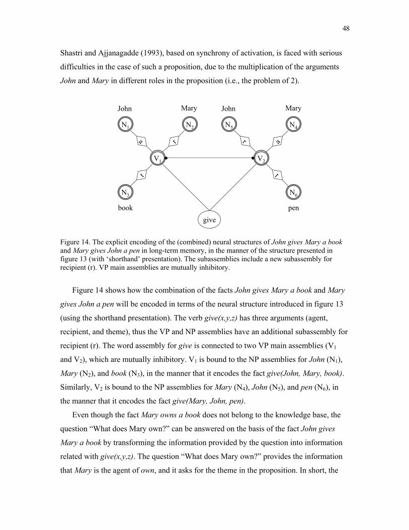
48
Shastri and Ajjanagadde (1993), based on synchrony of activation, is faced with serious
difficulties in the case of such a proposition, due to the multiplication of the arguments
John and Mary in different roles in the proposition (i.e., the problem of 2).
Figure 14. The explicit encoding of the (combined) neural structures of John gives Mary a book and Mary gives John a pen in long-term memory, in the manner of the structure presented in figure 13 (with ‘shorthand’ presentation). The subassemblies include a new subassembly for recipient (r). VP main assemblies are mutually inhibitory.
Figure 14 shows how the combination of the facts John gives Mary a book and Mary
gives John a pen will be encoded in terms of the neural structure introduced in figure 13
(using the shorthand presentation). The verb give(x,y,z) has three arguments (agent,
recipient, and theme), thus the VP and NP assemblies have an additional subassembly for
recipient (r). The word assembly for give is connected to two VP main assemblies (V1
and V2), which are mutually inhibitory. V1 is bound to the NP assemblies for John (N1),
Mary (N2), and book (N3), in the manner that it encodes the fact give(John, Mary, book).
Similarly, V2 is bound to the NP assemblies for Mary (N4), John (N5), and pen (N6), in
the manner that it encodes the fact give(Mary, John, pen).
Even though the fact Mary owns a book does not belong to the knowledge base, the
question “What does Mary own?” can be answered on the basis of the fact John gives
Mary a book by transforming the information provided by the question into information
related with give(x,y,z). The question “What does Mary own?” provides the information
that Mary is the agent of own, and it asks for the theme in the proposition. In short, the
t
V1
give
a r
t
V2
r a
N1 N5N2
N3
N4
N6
John Mary
book
John Mary
pen
49
question provides information of the form own(Mary, ?). In terms of give(x,y,z), the
question provides the information that Mary is the recipient of give, and it asks for the
theme in the proposition. In short, the question provides information of the form give(-,
Mary, ?). In general, information of the form own(X,?) can be transformed into
information of the form give(-,X,?) on the basis of a long-term association between own-
agent and give-recipient (as in the model of Shastri and Ajjanagadde, 1993).
In line with the process of answering binding questions (sections 6.3.1. and 6.3.2.),
the information of the form own(X, ?) will produce the activation of the assembly for own
and the gating circuits for agent. In contrast, the information of the form give(-,X, ?) will
produce the activation of the assembly for give and the gating circuits for recipient.
Therefore, the activation produced by own(X,?) cannot be concurrently active with the
activation produced by give(-,X,?). In figure 14, this would result in the activation of give
and the combined activation of the gating circuits for agent and recipient. The VP
assemblies V1 and V2 would then receive an equal amount of activation when the
assembly for X (Mary) is active, so that book and pen would have an equal probability of
being produced as the answer to the question.
Concurrent activation produced by own(X,?) and give(-,X,?) would be prevented if
the activation produced by own(X,?) consists of an ‘attractor’ state (Amit, 1989) of a
control network, which is associated with the attractor state in the control network
produced by give(-,X,?). First, the control network will be in the attractor state related
with own(X,?). But when an answer is not produced in this way (because own(Mary,
book) does not belong to the knowledge base), the attractor state in the control network
would change into the associated attractor state that corresponds with give(-,X,?)13.
When the information related with give(-, Mary, ?) is singled out, the answer can be
produced by activating Mary and give, and the gating circuit for recipient. As illustrated
in figure 14, this will result in V1 as the winner of the competition between the VP
assemblies (as in figure 8). After that, the answer can be produced by activating the
gating circuits for theme.
The transformation of the information related with own(X,?) into information related
with give(-,X,?) does not depend on Mary, or on any of the other word assemblies in
figure 14 (i.e., book, pen, or John). It only depends on the association between own-agent
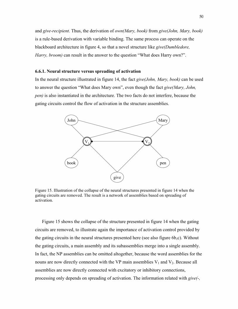
50
and give-recipient. Thus, the derivation of own(Mary, book) from give(John, Mary, book)
is a rule-based derivation with variable binding. The same process can operate on the
blackboard architecture in figure 4, so that a novel structure like give(Dumbledore,
Harry, broom) can result in the answer to the question “What does Harry own?”.
6.6.1. Neural structure versus spreading of activation
In the neural structure illustrated in figure 14, the fact give(John, Mary, book) can be used
to answer the question “What does Mary own”, even though the fact give(Mary, John,
pen) is also instantiated in the architecture. The two facts do not interfere, because the
gating circuits control the flow of activation in the structure assemblies.
Figure 15. Illustration of the collapse of the neural structures presented in figure 14 when the gating circuits are removed. The result is a network of assemblies based on spreading of activation.
Figure 15 shows the collapse of the structure presented in figure 14 when the gating
circuits are removed, to illustrate again the importance of activation control provided by
the gating circuits in the neural structures presented here (see also figure 6b,c). Without
the gating circuits, a main assembly and its subassemblies merge into a single assembly.
In fact, the NP assemblies can be omitted altogether, because the word assemblies for the
nouns are now directly connected with the VP main assemblies V1 and V2. Because all
assemblies are now directly connected with excitatory or inhibitory connections,
processing only depends on spreading of activation. The information related with give(-,
V1
book
give
John
V2
pen
Mary

51
Mary, ?) results in the activation of the assemblies for give and Mary. Due to the
uncontrolled spreading of activation, the activation of give and Mary results in an equal
activation of V1 and V2, so that a correct answer to the question cannot be given without
ambiguity or error.
In fact, any question will result in ambiguities or error in this uncontrolled spreading
of activation network. For instance, a question like “Who gives a book?” will result in the
activation of both John and Mary as potential answers, even though V1 will win the
competition over V2. In contrast, in the structure in figure 14, the question “Who gives a
book?” will result in John as the answer, because the question will result in the activation
of the gating circuits for agent after V1 has won the VP competition.
6.7. Summary of the basic architecture
The ability of the architecture to encode arbitrary sentence structures is based on the fact
that binding between a word assembly and a structure assembly, and between two
structure assemblies, is only temporal. The duration of the binding between two
assemblies is given by the duration of the reverberating activity of the delay assembly in
the memory circuit that connects the two assemblies. When the reverberating activity in
the delay assemblies disappears, the structure assemblies are ‘free’ again, which means
that they can be used to encode another sentence structure. Furthermore, only a small set
of structure assemblies is needed in the architecture (enough to account for the memory
span of language users and the duration of reverberating activity). As a result, an arbitrary
number of sentence structures can be encoded without an explosion of structure
assemblies.
Binding in this architecture is not a state of the system that needs to be observed for
read-out purposes (as in the case of binding with synchrony of activation). Instead, it is a
process, in which binding relations can be retrieved by posing ‘binding questions’. A
system can only answer a binding question on the basis of information that is available to
the system itself. Thus, the answer to a binding question shows that the system has solved
the binding problem implicated in the question. For instance, mouse is bound to chases as
its theme when it emerges as the answer of the question “Whom does the cat chase?”, as
illustrated in figures 7 and 8. The process of answering binding questions affects
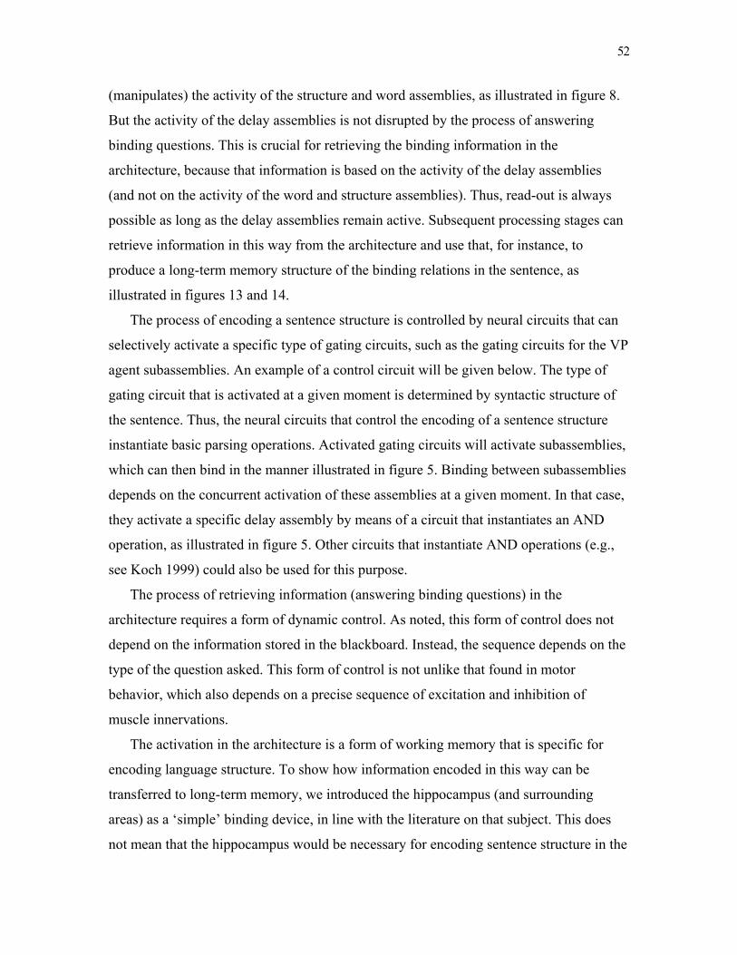
52
(manipulates) the activity of the structure and word assemblies, as illustrated in figure 8.
But the activity of the delay assemblies is not disrupted by the process of answering
binding questions. This is crucial for retrieving the binding information in the
architecture, because that information is based on the activity of the delay assemblies
(and not on the activity of the word and structure assemblies). Thus, read-out is always
possible as long as the delay assemblies remain active. Subsequent processing stages can
retrieve information in this way from the architecture and use that, for instance, to
produce a long-term memory structure of the binding relations in the sentence, as
illustrated in figures 13 and 14.
The process of encoding a sentence structure is controlled by neural circuits that can
selectively activate a specific type of gating circuits, such as the gating circuits for the VP
agent subassemblies. An example of a control circuit will be given below. The type of
gating circuit that is activated at a given moment is determined by syntactic structure of
the sentence. Thus, the neural circuits that control the encoding of a sentence structure
instantiate basic parsing operations. Activated gating circuits will activate subassemblies,
which can then bind in the manner illustrated in figure 5. Binding between subassemblies
depends on the concurrent activation of these assemblies at a given moment. In that case,
they activate a specific delay assembly by means of a circuit that instantiates an AND
operation, as illustrated in figure 5. Other circuits that instantiate AND operations (e.g.,
see Koch 1999) could also be used for this purpose.
The process of retrieving information (answering binding questions) in the
architecture requires a form of dynamic control. As noted, this form of control does not
depend on the information stored in the blackboard. Instead, the sequence depends on the
type of the question asked. This form of control is not unlike that found in motor
behavior, which also depends on a precise sequence of excitation and inhibition of
muscle innervations.
The activation in the architecture is a form of working memory that is specific for
encoding language structure. To show how information encoded in this way can be
transferred to long-term memory, we introduced the hippocampus (and surrounding
areas) as a ‘simple’ binding device, in line with the literature on that subject. This does
not mean that the hippocampus would be necessary for encoding sentence structure in the
53
architecture itself. Sentence encoding in the blackboard architecture can occur
independently of the hippocampus. In fact, the activity of the delay assemblies that
encodes a sentence structure in the blackboard is needed for the use of the hippocampus
as a simple binding device, as illustrated in figures 11 and 12.
6.8. Structural dependencies in the blackboard architecture
As Jackendoff (2002) noted, a solution of the ‘four challenges for cognitive
neuroscience’, as presented above, would allow a more productive interaction between
neural network modeling and linguistic theory to begin. To illustrate the possibility of
such an interaction, we will discuss the neural blackboard structures of the sentences (1)
and (2), discussed in section 4.2. They are repeated here for convenience:
The cat that the dog that the boy likes bites chases the mouse (1)
The fact that the mouse that the cat chases roars surprises the boy (2)
In section 4.3, we argued that these two sentences pose a problem for models that
process sentences in terms of strings of word category labels (N-V strings). Both
sentences have the same word category structure (N-that-N-that-N-V-V-V-N), but they are
different in terms of complexity (Gibson 1998), with (1) rated as far more complex than
(2). The difference in complexity between the sentences is related with the different
bindings between the constituents in both sentences. In (1) the subject of the main clause
(cat) is also an argument (theme) of a verb in an embedded clause (bites), whereas in (2)
the subject of the main clause (fact) is not an argument of any of the verbs in the
embedded clauses (chases and roars). The contrast between (1) and (2) forms an
interesting example of the massiveness of the binding problem that occurs in language.
A neural instantiation of sentence structure has to account for the differences in
constituent binding illustrated with sentences (1) and (2), as any linguistic theory of
sentence structure would have to do. But a neural instantiation of sentence structure
should also provide an explanation of the observed differences in complexity between
these sentences (and other performance effects, Van der Velde 1995).

54
As noted, the structural difference between sentences (1) and (2) is related with the
nature of the embedded clauses they contain. Therefore, we first have to discuss how
embedded clauses can be instantiated in the neural architecture presented here.
6.8.1. Embedded clauses in the blackboard architecture
Figure 16a presents the structure of the sentence The cat that bites the dog chases the
mouse (without the determiners the). This sentence contains the subject-relative clause
that bites the dog. To encode and bind this clause, a new clause structure assembly (C) is
introduced, with a new clause subassembly (c). C assemblies play a role in the encoding
of a clause that is similar to the role played by S assemblies in the encoding of the main
sentence (cat chases mouse in figure 16a). However, there are a few differences between
the role played by S and C assemblies, which motivates their distinction14. C assemblies
have to be bound to one of the structure assemblies in the sentence, as illustrated with the
binding between C1 and N1 in figure 16a, which requires a new kind of subassembly (c).
Furthermore, the word assemblies of complementizers can bind with C assemblies, as
illustrated with that in figure 16a.
A verb (verb-phrase) can only have a single argument for each of its thematic roles,
but a noun (noun-phrase) can be the argument of two verbs. That is, a noun can bind to
the verb on the same level as the noun in the sentence structure (the ‘sister’ of the noun),
and it can bind to a verb in a subordinate clause. Because binding is achieved with
subassemblies in this architecture, different subassemblies will be needed for binding a
noun with its ‘sister’ verb and with a subordinate verb. In figure 16a, to encode that cat is
the subject of the verb in its subordinate clause (bites the dog), N1 binds with a nc (noun-
clause) subassembly to the n subassembly of C1. The nc subassembly of N1 is similar to
its n subassembly, except that it is activated under the influence of the (subordinate)
clause C1, introduced with that.
Like S assemblies, C assemblies can be used to encode agreement between subject
and verb. In the case of a subject-relative clause, agreement exists between subject of the
main sentence (cat) and the verb of the relative clause (bites), as indicated with the dotted
line between the noun and verb subassemblies of the C assembly in figure 16a.
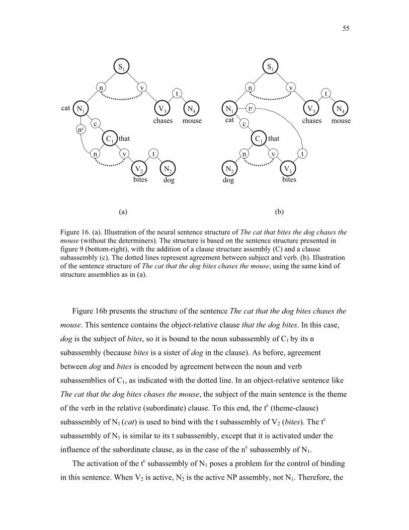
55
Figure 16. (a). Illustration of the neural sentence structure of The cat that bites the dog chases the mouse (without the determiners). The structure is based on the sentence structure presented in figure 9 (bottom-right), with the addition of a clause structure assembly (C) and a clause subassembly (c). The dotted lines represent agreement between subject and verb. (b). Illustration of the sentence structure of The cat that the dog bites chases the mouse, using the same kind of structure assemblies as in (a).
Figure 16b presents the structure of the sentence The cat that the dog bites chases the
mouse. This sentence contains the object-relative clause that the dog bites. In this case,
dog is the subject of bites, so it is bound to the noun subassembly of C1 by its n
subassembly (because bites is a sister of dog in the clause). As before, agreement
between dog and bites is encoded by agreement between the noun and verb
subassemblies of C1, as indicated with the dotted line. In an object-relative sentence like
The cat that the dog bites chases the mouse, the subject of the main sentence is the theme
of the verb in the relative (subordinate) clause. To this end, the tc (theme-clause)
subassembly of N1 (cat) is used to bind with the t subassembly of V2 (bites). The tc
subassembly of N1 is similar to its t subassembly, except that it is activated under the
influence of the subordinate clause, as in the case of the nc subassembly of N1.
The activation of the tc subassembly of N1 poses a problem for the control of binding
in this sentence. When V2 is active, N2 is the active NP assembly, not N1. Therefore, the
N1
n
S1
V3
t
N4
v
c
C1
N2V2
tv
cat
bites
chases mouse
that
dog
(a) (b)
N1
n
S1
V3
t
N4
v
c
C1
N2
n
V2
tv
cat
bites
chases mouse
that
dog
tc
nc
n

56
tc subassembly of N1 has to be activated before the activation of N2 (a subassembly can
remain active even if its main assembly is deactivated). Thus, the gating circuits for
theme-clause have to be activated before the activation of the main assembly of N2. With
the object-relative sentence in figure 16b, the control circuits could conclude from the
sequence cat that dog (or N that N) that cat is the theme of a verb in the clause, so that
the gating circuits for tc have to be activated before the activation of N2. This control of
activation is not needed for the subject-relative sentence in figure 16a. Furthermore, the
theme of bites (V2) in figure 16a presents itself directly with the occurrence of dog (N2),
resulting in a direct binding between V2 and N2. In figure 16b, the theme of bites (cat-N1)
can only bind with V2 due to the prolonged activation of tc. These activation differences
between the structures in figure 16b and figure 16a could be the basis for the fact that
object-relative sentences are more difficult to process than subject-relative sentences
(Gibson 1998).
Because a verb can have only one argument, the distinction between t and tc
subassemblies needed for NP assemblies does not occur with VP assemblies. For the
same reason, the distinction between n and nc subassemblies needed for NP assemblies
does not occur with C assemblies. In this way, the verb bites can have only one subject
(either cat-N1 in figure 16a or dog-N2 in figure 16b) and only one theme (either dog-N2 in
figure 16a or cat-N1 in figure 16b).
In case of a sentence The cat that the dog bites chases the mouse (figure 16b), the
question “Who bites the cat that chases the mouse?” can be answered by activating the
word assemblies, and the gating circuits in the direction from mouse (theme) to chases
(subject) to cat (theme) to bites. This will result in bites (V2) winning the competition (in
particular, because it receives more activation from cat (N1) than chases (V3) receives
from mouse (N4).
An interesting comparison can be made with answering the question “Whom does the
cat that chases the mouse bite?” with the sentence The cat that bites the dog chases the
mouse (figure 16a). The difficulty here is that cat is both the subject (agent) of chases and
bites. So, it has to be figured out that cat bites dog is an embedded clause, that is, that
activating the gating circuits in the direction from mouse to chases to cat results in the
activation of the S assembly instead of the C assembly. In other words, the architecture
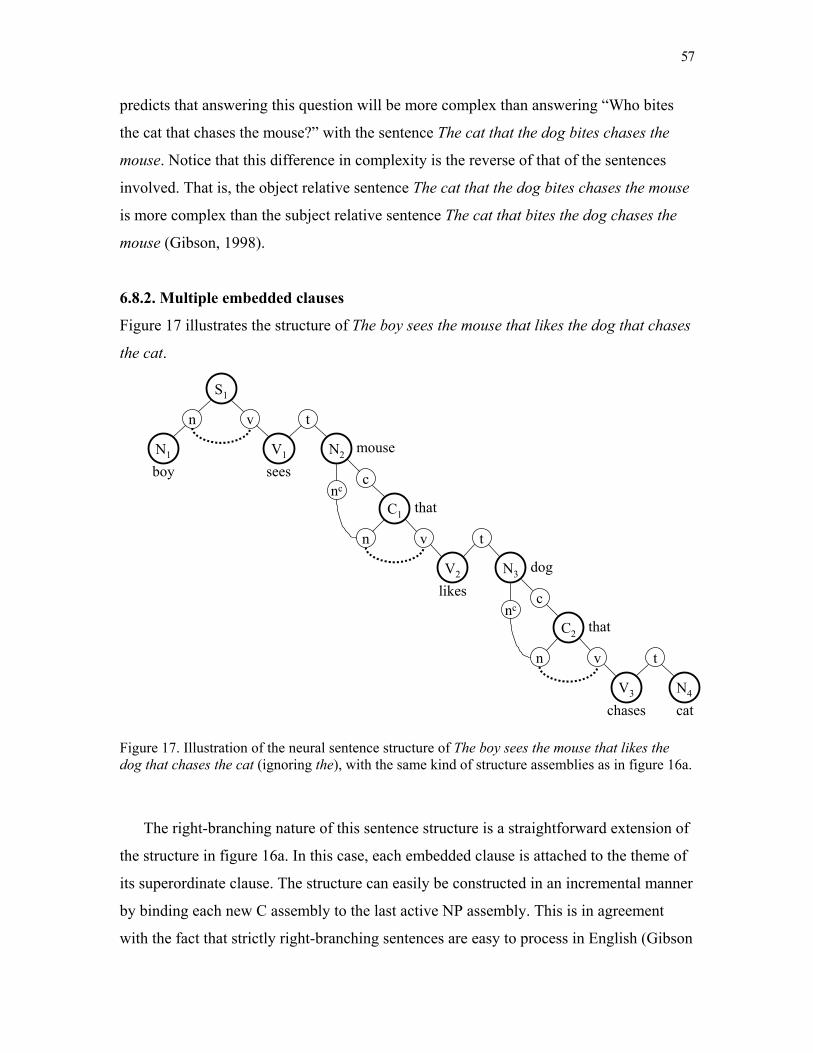
57
predicts that answering this question will be more complex than answering “Who bites
the cat that chases the mouse?” with the sentence The cat that the dog bites chases the
mouse. Notice that this difference in complexity is the reverse of that of the sentences
involved. That is, the object relative sentence The cat that the dog bites chases the mouse
is more complex than the subject relative sentence The cat that bites the dog chases the
mouse (Gibson, 1998).
6.8.2. Multiple embedded clauses
Figure 17 illustrates the structure of The boy sees the mouse that likes the dog that chases
the cat.
Figure 17. Illustration of the neural sentence structure of The boy sees the mouse that likes the dog that chases the cat (ignoring the), with the same kind of structure assemblies as in figure 16a.
The right-branching nature of this sentence structure is a straightforward extension of
the structure in figure 16a. In this case, each embedded clause is attached to the theme of
its superordinate clause. The structure can easily be constructed in an incremental manner
by binding each new C assembly to the last active NP assembly. This is in agreement
with the fact that strictly right-branching sentences are easy to process in English (Gibson
S1
N1
n
V1
v
boyN2
sees
C1
V2
v
that
c
n
N3
C2
c
chases
that
t
mouse
likes
t
nc
dog
catV3
tv
N4
n
nc
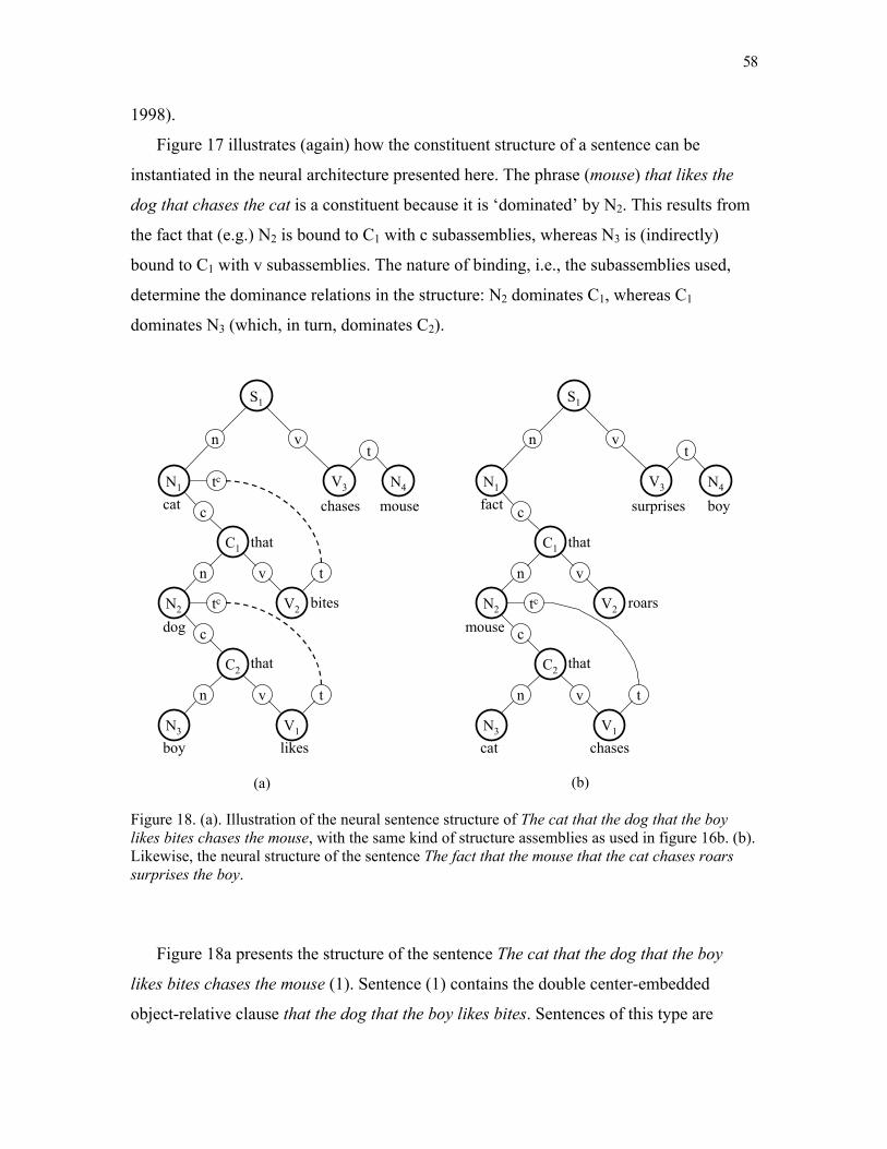
58
1998).
Figure 17 illustrates (again) how the constituent structure of a sentence can be
instantiated in the neural architecture presented here. The phrase (mouse) that likes the
dog that chases the cat is a constituent because it is ‘dominated’ by N2. This results from
the fact that (e.g.) N2 is bound to C1 with c subassemblies, whereas N3 is (indirectly)
bound to C1 with v subassemblies. The nature of binding, i.e., the subassemblies used,
determine the dominance relations in the structure: N2 dominates C1, whereas C1
dominates N3 (which, in turn, dominates C2).
Figure 18. (a). Illustration of the neural sentence structure of The cat that the dog that the boy likes bites chases the mouse, with the same kind of structure assemblies as used in figure 16b. (b). Likewise, the neural structure of the sentence The fact that the mouse that the cat chases roars surprises the boy.
Figure 18a presents the structure of the sentence The cat that the dog that the boy
likes bites chases the mouse (1). Sentence (1) contains the double center-embedded
object-relative clause that the dog that the boy likes bites. Sentences of this type are
N1
n
S1
V3
t
N4
v
c
C1
N2
n
V2
v
fact
mouseroars
surprises boy
that
C2
V1
tv
chases
that
c
n
N3
cat
tc
N1
n
S1
V3
t
N4
v
c
C1
N2
n
V2
tv
cat
dogbites
chases mouse
that
C2
V1
tv
likes
that
c
n
N3
boy
tc
tc
(a) (b)
59
notoriously hard to process, to the point that they can be classified as unprocessable
(Gibson 1998). The encoding of the phrase The cat that the dog proceeds in the same way
as in figure 16b, so that the tc subassembly of N1 (cat) will be activated to bind with the
theme subassembly of the next verb. However, another embedded clause is introduced,
instead of a verb. The phrase the dog that the boy is structurally similar to the phrase the
cat that the dog, so that the tc subassembly of N2 (dog) will be activated to bind with the
theme subassembly of the next verb. Thus, when the first verb (likes) appears, there are
two subassemblies that can bind with the theme subassembly of this verb, whereas the
verb should bind with dog (N2) as its theme argument. The situation is similar with the
second verb (bites), which should bind with cat (N1) as its theme argument. The two
problematic bindings are indicated with the dashed lines in figure 18a.
Figure 18b shows the structure of the sentence The fact that the mouse that the cat
chases roars surprises the boy (2). The structure of (2) is very similar to the structure of
(1), except for the fact that roars (V2) does not have a theme argument. A phrase
beginning with The fact that will be interpreted as a complementary clause, so that the tc
subassembly of N1 (fact) will not be activated. When the object-relative clause in the
mouse that the cat chases appears, the tc subassembly of N2 (mouse) will be activated to
bind mouse as the theme of the verb in its subordinate clause (chases), as in figure 16b.
However, in contrast with the structure of (1) in figure 18a, the binding of mouse (N2)
with the first verb (chases) as its theme can succeed because the theme subassembly of
N2 is the only active theme subassembly at that moment.
Thus the difference in complexity between (1) and (2) results from a difference in
structural dependency between both sentences. In (1) the subject of the main sentence
(cat) is also the theme of a verb in an object-relative clause. In combination with the
second object-relative clause, this results in an ambiguity of the binding of cat (N1) or
dog (N2) as the theme of likes (V1) or bites (V2). In contrast, in (2) the subject of the main
clause (fact) is not bound to any of the verbs in the embedded clauses, so that the
ambiguities in (1) do not arise in (2). Hence, sentence complexity in (1) results from
binding problems that arise when a number of structure assemblies of the same kind have
to bind in sequence with the overall sentence structure (in line with the notion of
similarity-based interference as the basis of sentence complexity, Lewis 1999)
60
At face value, the binding problem that arises with the theme subassemblies of the
sentence structure in figure 18a would also have to arise with the verb subassemblies in
both sentence structures in figure 18, in particular for the verb subassemblies connected
to the C assemblies (the verb subassembly of the S assembly could be activated after the
binding of C assemblies has been completed). The activation of C2 will inhibit the
activation of C1 in both sentence structures, thus the verb subassembly of C1 has to be
activated before C2 is activated. But the first verb in the sentence (likes or chases) has to
be bound to C2, which requires the activation of the verb subassembly of C2 as well.
However, the binding problem with the verb subassemblies can be solved in terms of the
dynamics of the binding process, as discussed below.
6.8.3. Dynamics of binding in the blackboard architecture
The binding of subassemblies occurs in a connection structure as illustrated in figure 5.
Figure 19 illustrates the process of subassembly binding between two arbitrary structure
assemblies A and B.
In figure 19a, the subassembly of Ai-1 has activated its horizontal row of columns in
the connection structure. If the Bj subassembly would activate its vertical row of columns
in the connection structure, a binding would result between Ai-1 and Bj, in the manner as
discussed in section 6.2.1. However, the subassembly of Ai is activated first, which
results in the activation of a second horizontal row of columns.
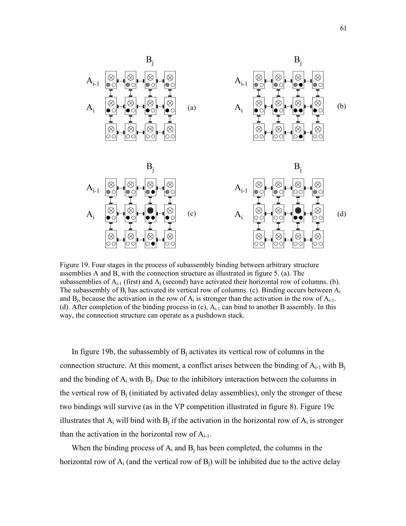
61
Figure 19. Four stages in the process of subassembly binding between arbitrary structure assemblies A and B, with the connection structure as illustrated in figure 5. (a). The subassemblies of Ai-1 (first) and Ai (second) have activated their horizontal row of columns. (b). The subassembly of Bj has activated its vertical row of columns. (c). Binding occurs between Ai and Bj, because the activation in the row of Ai is stronger than the activation in the row of Ai-1. (d). After completion of the binding process in (c), Ai-1 can bind to another B assembly. In this way, the connection structure can operate as a pushdown stack.
In figure 19b, the subassembly of Bj activates its vertical row of columns in the
connection structure. At this moment, a conflict arises between the binding of Ai-1 with Bj
and the binding of Ai with Bj. Due to the inhibitory interaction between the columns in
the vertical row of Bj (initiated by activated delay assemblies), only the stronger of these
two bindings will survive (as in the VP competition illustrated in figure 8). Figure 19c
illustrates that Ai will bind with Bj if the activation in the horizontal row of Ai is stronger
than the activation in the horizontal row of Ai-1.
When the binding process of Ai and Bj has been completed, the columns in the
horizontal row of Ai (and the vertical row of Bj) will be inhibited due to the active delay
(a)
(c)
(b)
(d)
Ai
Ai-1
Ai
Ai-1
Ai
Ai-1
Ai
Ai-1
Bj
Bj
Bj
Bj
62
assembly in the column that binds Ai with Bj. However, as illustrated in figure 19d, the
columns in the horizontal row of Ai-1 are still active (with the exception of the column in
the vertical row of Bj). Thus, the subassembly of Ai-1 can bind with another B
subassembly if that is activated.
The process illustrated in figure 19 shows that two A subassemblies can bind in
sequence with B subassemblies if there is a clear difference in activation strength
between the two A subassemblies. In that case, the stronger activated A subassembly will
bind with the first activated B subassembly and the other A subassembly will bind with
the second activated B subassembly. In theory, one could have a whole series of A
subassemblies that can bind in sequence with B subassemblies, if the A subassemblies
have distinguishable differences in their activation strengths.
Pulvermüller (1999) suggested that a gradual decay of activation in reverberating
assemblies (such as the delay assemblies in the memory circuits) could form the basis of
a neural pushdown stack. Figure 19 illustrates this possibility. If the subassemblies of Ai-n
to Ai have been activated that order, and if the activation strength of the subassemblies
decays over time, then the subassembly of Ai would have the strongest activation and it
would bind to the first B subassembly, as illustrated in figure 19. Then, the subassembly
of Ai-1 would bind to the next B subassembly, as illustrated in figure 19d. In the same
manner, all the subassemblies of Ai-n to Ai would bind to B subassemblies in the reverse
order of their activation, in line with the notion of a pushdown stack15.
It is not clear whether such a distinctive and reliable decay of reverberating activity
will be found in the brain, due to the fluctuations that can occur in this kind of activity
(Amit 1989). However, in one circumstance one can find a clear difference in activation
strength between reverberating assemblies. Fuster et al. (1985) investigated the relation
between reverberating activity in the prefrontal cortex and the visual cortex. First, they
identified neurons in both areas of the cortex that responded to the same objects and that
maintained their activation in a delay period. Then, they applied a technique of reversible
cooling to one of the areas involved. In this way, the activity of the neurons in that area
can be blocked temporarily, but the activity will reappear when the temperature is
increased to a normal level. Fuster et al. (1985) observed that blocking the activity of
neurons in one area also reduced the activity of the neurons in the other area. The activity

63
in the second area increased again when the activity in the first area reappeared (by
terminating the cooling in that area).
The results of Fuster et al. (1985) indicate that reverberating activity in a neural
assembly is stronger when the assembly also receives activation from outside. In this
way, the binding of the verb subassemblies in the sentence structures in figure 18 can be
explained. The main assembly of C2 is active when the first verb (likes or chases)
appears. Therefore, the verb subassembly of C2 is also activated by the main assembly,
unlike the verb subassembly of C1. As a result, the activity of the verb subassembly of C2
is stronger than the activity of the verb subassembly of C1. In line with the binding
process illustrated in figure 19, the verb subassembly of C2 will bind with the verb
subassembly of V1 (likes or chases), and the verb subassembly of C1 will bind with the
VP assembly (V2) of the next verb (bites or roars).
In contrast, the main assembly of N2 in figure 18a is not active, due to the activation
of N3 (boy), which is needed to bind boy with likes. Without a clear distinction in
activation strength between the theme subassemblies of N1 and N2, the binding process
illustrated in figure 19 will produce a conflict, which results in the complexity associated
with sentence (1).
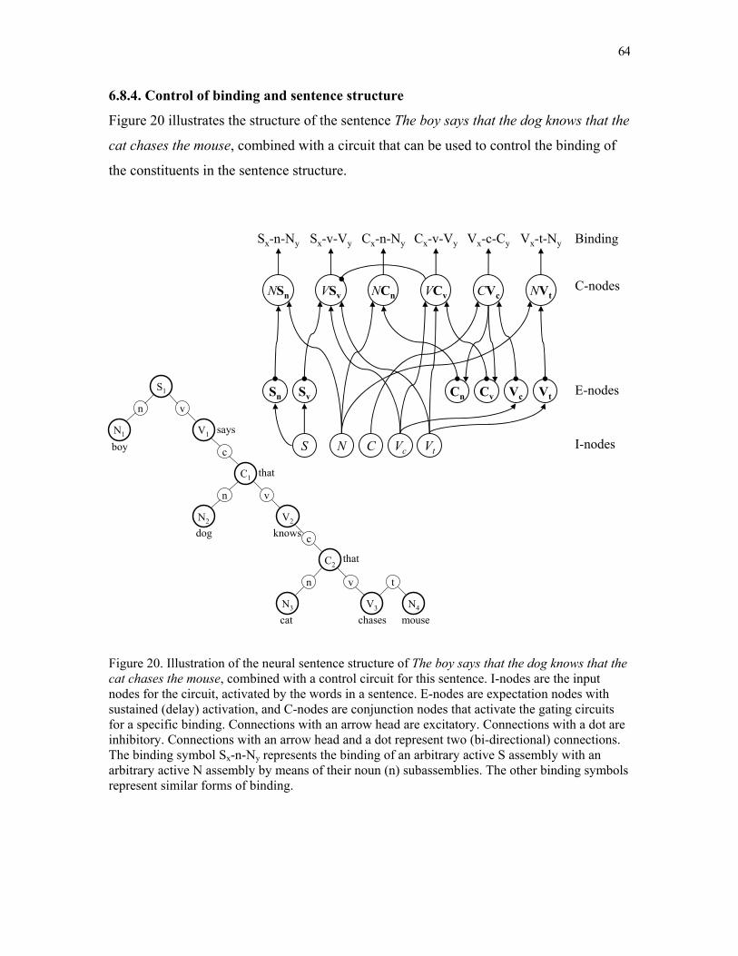
64
6.8.4. Control of binding and sentence structure
Figure 20 illustrates the structure of the sentence The boy says that the dog knows that the
cat chases the mouse, combined with a circuit that can be used to control the binding of
the constituents in the sentence structure.
Figure 20. Illustration of the neural sentence structure of The boy says that the dog knows that the cat chases the mouse, combined with a control circuit for this sentence. I-nodes are the input nodes for the circuit, activated by the words in a sentence. E-nodes are expectation nodes with sustained (delay) activation, and C-nodes are conjunction nodes that activate the gating circuits for a specific binding. Connections with an arrow head are excitatory. Connections with a dot are inhibitory. Connections with an arrow head and a dot represent two (bi-directional) connections. The binding symbol Sx-n-Ny represents the binding of an arbitrary active S assembly with an arbitrary active N assembly by means of their noun (n) subassemblies. The other binding symbols represent similar forms of binding.
S1
N1
n
V1
v
boysays
C1
V2
v
that
c
n
N2
dog
mouse
C2
V3
tv
chases
that
c
n
N3
cat
knows
N4
VtVcN CS
VcSvSn Cn Cv Vt
VSv CVcNCn VCvNSn NVt
I-nodes
E-nodes
C-nodes
Sx-n-Ny Sx-v-Vy Cx-v-VyCx-n-Ny Vx-c-Cy Vx-t-Ny Binding
65
The control circuit is given in the form of a connectionist network consisting of I-
nodes (input nodes), E-nodes (‘expectation’ nodes), and C-nodes (‘conjunction’ nodes).
The I-nodes are activated by the words in the sentence, based on their lexical type. It is
assumed that one I-node is active at a time (with the exception of the I-node S). The I-
node S is inhibited by the E-nodes (not shown in figure 20). The E-nodes are activated by
specific I-nodes or C-nodes. They remain active until inhibited. The C-nodes are
activated by a specific conjunction of an I-node and an E-node. They activate the gating
circuits that result in a specific binding of constituents in the sentence structure, and they
inhibit the E-node by which they are activated.
When boy is presented, it binds with N1 and it activates the I-node N. Furthermore,
boy will be seen as the beginning of a sentence, because there are no active E-nodes that
would force a binding of boy in an existing sentence structure (see below). As a result,
boy also activates S1 and the I-node S, which in turn activates the E-nodes Sn and Sv. The
conjunction node NSn is then activated, which results in the binding of S1 and N1 with
their noun (n) subassemblies. The activation of the E-node Sv reflects the expectation of a
verb for the main (matrix) sentence.
When the verb says is presented, it activates V1 and the I-node Vc, which entails that
says is interpreted as a verb that requires a complement clause (given by the lexical
information related with says). In turn, Vc activates the expectation node Vc. The
combined activation of the I-node Vc and the E-node Sv results in the activation of the
conjunction node VSv. This node activates the gating circuits for the binding of V
assemblies and S assemblies with their verb (v) subassembly, which results in the binding
of V1 with S1. The word that activates C1 and the I-node C, which in combination with
the E-node Vc activates the C-node CVc. In turn, CVc produces the binding of C1 with V1,
and activates the E-nodes Cn and Cv (i.e., the expectation of a clause subject and verb).
Continuing in this manner, dog (N2) and knows (V2) will bind with C1. The verb
knows again activates the I-node Vc, which results in the binding of that (C2) with knows
(V2). Then, cat (N3) and chases (V3) will bind with C2. The verb chases is a verb that
requires a theme. This lexical information related with chases will activate the I-node Vt,
which in turn activates the E-node Vt. The word mouse will bind with N4 and will
activate the I-node N. In combination with the active E-node Vt, this results in the
66
binding of mouse (N4) as the theme of chases (V3). Notice that the nouns dog, cat and
mouse are bound in an existing sentence structure due to the active expectation nodes in
the circuit.
The circuit in figure 20 illustrates how the process of binding could proceed in the
architecture for sentence structure presented here. However, it is clear that a more
detailed account of this process is a topic for further research, as described below.
6.9. Further development of the architecture
The neural blackboard architecture for sentence structure outlined here provides a
solution to the ‘four challenges for cognitive neuroscience’ presented by Jackendoff
(2002). The discussion in section 6.8 also illustrates that the architecture can potentially
account for structural and performance aspects of language processing. However, further
research is clearly needed to provide a more complete fulfillment of this potential. A few
directions of further research can be indicated with the architecture presented thus far.
One line of research would concern the development of the architecture, both in terms
of evolution and in terms of growth and learning. As figure 7a illustrates, the architecture
consists for the most part of gating circuits, which can be seen as the first level of
organization in the architecture. The second level consists of gating circuits organized in
structure assemblies. The third level of organization consists of the distinction between
different kinds of structure assemblies and the way they interact. Gating mechanisms are
found in the brain (e.g., Newman et al. 1997). So, the study of the development of the
architecture would be focused on the way in which the second and third level of
organization arise.
In terms of evolution, an important issue is the development of the connection
structure presented in figures 5 and 19. A benefit of an explicit model as the one in figure
5 is that the model can be used as a target in computer simulations. Thus, starting with
more elementary structures, one could investigate whether such a connection structure
could develop in an evolution-like process. In terms of growth and learning, an important
issue is the question of how specific bindings with connection structures like the one in
figure 5 could develop. That is, assuming that an undifferentiated connection structure
exists for undifferentiated assemblies, one can investigate whether a learning process
67
could reorganize the undifferentiated connection structure into a connection structure in
which distinctions are found between different kinds of structure assemblies and
subassemblies, as illustrated above. Furthermore, one could investigate whether different
languages used in the learning process would result in a different reorganization of the
initial connection structure.
Another line of research concerns the issue of parsing in this architecture. Parsing will
result from the neural circuits that control the binding process in the architecture. An
example is presented in figure 20. As noted earlier, the control circuits instantiate basic
parsing operations. Thus, they will be sensitive to the coding principles used in languages
to express structural information, like word order, or case marking in languages with free
word order (Van Valin 2001). However, the neural control circuits will also be sensitive
to the pattern of activation that arises in the blackboard during sentence processing.
Figure 19 provides an illustration. An active subassembly produces a significant amount
of activation in its connection structure (i.e., its row of columns), which provides the
information that a specific binding is required. This information can be used by the
control circuits to initiate the activation of a subassembly of the same kind (e.g., a VP
theme subassembly when a NP theme subassembly active).
One topic in the study of parsing will be the question of how constraints are
implemented in the control circuits, and how they relate with aspects of sentence
ambiguity. An example of a constraint is presented in the circuit in figure 20. It consists
of the inhibitory connection from the C-node VCv to the C-node VSv. This connection
implements the hierarchical constraint that verb-binding in a clause precedes verb-
binding in a main (matrix) sentence (as in figure 18). This form of constraint is a ‘hard’
constraint in which one demand (verb-binding in a clause) overrides another (verb-
binding in a matrix sentence). An important issue will be how ‘soft’ constraints can be
implemented, including those given by statistical regularities and semantic information.
It is clear that the study of parsing in the architecture presented here is just beginning.
However, the examples illustrated thus far suggest that the neural control circuits that
control the binding process in the architecture are engaged in a form of pattern
recognition and pattern completion, in which the current state of activation in the
blackboard together with the active word assemblies constitute the input pattern and the

68
new state of activation in the blackboard constitutes the output pattern. Pattern
recognition is a core capability of networks (Bechtel & Abrahamsen 2002). The fact that
a neural blackboard architecture of sentence structure could transform parsing operations
into forms of pattern recognition is an attractive prospect of further research.
In combination with parsing, the study of sentence complexity and other
psycholinguistic effects is also an important line of further research. Figures 16 and 18
illustrate the potential of the architecture to account for complexity effects, but there are
number of other complexity issues that should be accounted for as well (e.g., see Gibson,
1998). An interesting topic here will be the complexity related with answering binding
questions, as discussed in section 6.8.1. The architecture we presented suggests that this
can be a source of complexity of its own, that needs to be investigated further.
A fourth line of investigation consists of relating the structure and dynamics of the
architecture with observable brain structure and activation. The connection structure in
figure 5 is a prediction of how the brain could realize combinatorial productivity. The
activation in the architecture during sentence encoding, as illustrated in figure 7a, is also
a prediction of activation that would occur in the brain. Dynamic causal modeling
(Friston et al. 2003) can be used to compare activation simulated in a model with
activation observed with neuroimaging. As an example, this approach could be used to
investigate the sustained activation needed to handle long-distance dependencies. Figure
20 illustrates a long-distance dependency with object-relative clauses in the architecture,
which can be simulated in terms of the neural dynamics illustrated in figure 8. Ben-
Sachar et al. (2003) observed activation in specific brain regions produced by sentences
of this type (as compared with sentences with complement clauses). With the approach of
dynamic causal modeling, we can begin to compare the activation in the architecture
produced by these sentence types with the activation observed in the brain.
Likewise, the neural activity that occurs in a simulation, as illustrated in figure 7a,
can be transformed mathematically into an EEG signal, and compared with observations.
This is technically demanding, but in conceptual terms it can be done. An important issue
here is the topology of the network, which will affect the EEG signal. The model could
be used to test and develop specific topologies, by deriving the imaging signal using a
given topology and comparing it with empirical results.
69
A fifth line of research is the relation between the architecture for sentence structure
and other architectures for combinatorial structures in language (Jackendoff 2002) and
cognition in general. For instance, words can have an internal structure of their own,
which does not seem to agree with word encoding by means of (unstructured) word
assemblies (Bierwisch 1999). However, the word assemblies used here can be seen as the
interface between word structure (e.g., phonological structure) and sentence structure.
That is, a word assembly is the part of a neural word structure that connects (or
‘anchors’) that structure within the sentence structure. An example is given in figures 2
and 13, in which the assemblies for cat, chases and mouse form the interface between
sentence structures in working memory (figure 2) and sentence structures long-term
memory (figure 13).
The interaction between a neural architecture for combinatorial (e.g., phonological)
word structure and a neural architecture for sentence structure could explain how new
words can be embedded easily in a sentence structure. A new word is itself a novel
combination of familiar constituents (phonemes), instantiated in its own (assumed)
phonological neural blackboard. Thus, a new word would create a word structure in this
word architecture similar to the way in which a new sentence creates a sentence structure
in the neural sentence architecture. In this way, a new word would be temporarily
encoded with (say) a Wx assembly, just like a sentence is temporarily encoded with an Sx
assembly. The Wx assemblies could bind with the structure assemblies in the sentence
architecture, which would result in the embedding of the new word in the sentence
structure. Over time, the new word would form a direct link with the kind of structure
assemblies in the sentence architecture to which it belongs.
Word assemblies could also form the interface between sentence structures and
cognitive structures outside language, such as structures in visual cognition. This issue is
addressed in more detail below.
7. Neural blackboard architectures of combinatorial structures in vision
The aim of this paper is to show that combinatorial structures can be encoded in neural
terms by means of neural ‘blackboard’ architectures. Although combinatorial structures
are the ‘quintessential property’ of language (Pinker 1998), they can also be found in
70
visual cognition. Therefore, we will briefly discuss neural blackboard architectures of
combinatorial structures in visual cognition, in particular for binding visual object
features like shape, color and (relative) location. In this way we can investigate the
differences and similarities that exist between neural architectures of combinatorial
structures in two different domains like language and vision. Furthermore, we will
discuss how the architectures for visual cognition and language can be combined in a
combinatorial structure like The little star is beside a big star.
As in the case of the architecture for sentence structure, we will discuss the issue of
binding in the ‘vision’ architecture, such as the binding of color and shape, in terms of the
process that answers binding questions, like “What is the color of this shape?”. The
reason why we discuss the binding problem in this way is related with the coordinate
system or frame of reference in which the binding problem should be solved. As outside
observers, we could see some form of related (e.g., concurrent ) activity in brain areas
that are involved in processing information in a given task, such as binding the color and
shape of visual objects. But it is not clear that the observed relation in activity is used by
these brain areas to solve the binding problem at hand. That is, it is not clear that these
brain areas ‘know’ that they are (say) concurrently active with each other, so that they
can use that information effectively. What is needed is information that is available
within the system itself (instead of only from an outside perspective). A binding question
like “What is the color of this shape?” probes for information that is available within the
system itself, because the system generates behavior when it answers such a question,
which it can only do by using information that is available within the system itself.
Investigating the process that results in answering binding questions is, in our view, the
best way to study (and solve) the issue of binding in combinatorial structures, including
the binding of color and shape (and the binding of words in a sentence structure).
In a blackboard architecture for visual cognition, one would have processors for the
recognition of shape, color, location and other visual object features. Combined, these
processors would correctly process a visual display of objects, such as a blue cross on the
left and a yellow diamond on the right, if they could communicate with each other
through a blackboard. In this way, the architecture could answer binding questions like
“What is the color of the cross?" or "What is the shape of the yellow object?".
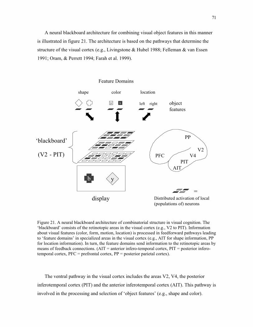
71
A neural blackboard architecture for combining visual object features in this manner
is illustrated in figure 21. The architecture is based on the pathways that determine the
structure of the visual cortex (e.g., Livingstone & Hubel 1988; Felleman & van Essen
1991; Oram, & Perrett 1994; Farah et al. 1999).
Figure 21. A neural blackboard architecture of combinatorial structure in visual cognition. The ‘blackboard’ consists of the retinotopic areas in the visual cortex (e.g., V2 to PIT). Information about visual features (color, form, motion, location) is processed in feedforward pathways leading to ‘feature domains’ in specialized areas in the visual cortex (e.g., AIT for shape information, PP for location information). In turn, the feature domains send information to the retinotopic areas by means of feedback connections. (AIT = anterior infero-temporal cortex, PIT = posterior infero-temporal cortex, PFC = prefrontal cortex, PP = posterior parietal cortex).
The ventral pathway in the visual cortex includes the areas V2, V4, the posterior
inferotemporal cortex (PIT) and the anterior inferotemporal cortex (AIT). This pathway is
involved in the processing and selection of ‘object features’ (e.g., shape and color).
(V2 - PIT)
y b
b y
display
‘blackboard’
left right
V2V4
PITAIT
PP
Feature Domains
objectfeatures
shape color location
PFC
Distributed activation of local (populations of) neurons
=
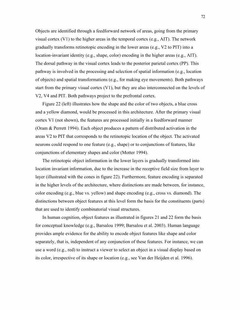
72
Objects are identified through a feedforward network of areas, going from the primary
visual cortex (V1) to the higher areas in the temporal cortex (e.g., AIT). The network
gradually transforms retinotopic encoding in the lower areas (e.g., V2 to PIT) into a
location-invariant identity (e.g., shape, color) encoding in the higher areas (e.g., AIT).
The dorsal pathway in the visual cortex leads to the posterior parietal cortex (PP). This
pathway is involved in the processing and selection of spatial information (e.g., location
of objects) and spatial transformations (e.g., for making eye movements). Both pathways
start from the primary visual cortex (V1), but they are also interconnected on the levels of
V2, V4 and PIT. Both pathways project to the prefrontal cortex.
Figure 22 (left) illustrates how the shape and the color of two objects, a blue cross
and a yellow diamond, would be processed in this architecture. After the primary visual
cortex V1 (not shown), the features are processed initially in a feedforward manner
(Oram & Perrett 1994). Each object produces a pattern of distributed activation in the
areas V2 to PIT that corresponds to the retinotopic location of the object. The activated
neurons could respond to one feature (e.g., shape) or to conjunctions of features, like
conjunctions of elementary shapes and color (Motter 1994).
The retinotopic object information in the lower layers is gradually transformed into
location invariant information, due to the increase in the receptive field size from layer to
layer (illustrated with the cones in figure 22). Furthermore, feature encoding is separated
in the higher levels of the architecture, where distinctions are made between, for instance,
color encoding (e.g., blue vs. yellow) and shape encoding (e.g., cross vs. diamond). The
distinctions between object features at this level form the basis for the constituents (parts)
that are used to identify combinatorial visual structures.
In human cognition, object features as illustrated in figures 21 and 22 form the basis
for conceptual knowledge (e.g., Barsalou 1999; Barsalou et al. 2003). Human language
provides ample evidence for the ability to encode object features like shape and color
separately, that is, independent of any conjunction of these features. For instance, we can
use a word (e.g., red) to instruct a viewer to select an object in a visual display based on
its color, irrespective of its shape or location (e.g., see Van der Heijden et al. 1996).
73
Figure 22. The process of answering the binding question “What is the color of the cross?” in the neural blackboard architecture of figure 21. Left: The shapes, cross and diamond, and the colors, blue (b) and yellow (y), of two objects are processed in feedforward pathways in the retinotopic areas. The receptive field size of neurons increases in higher areas (as indicated with the cones), until encoding is location invariant in the feature domains. Middle: The shape of the target object (the cross) is selected as a cue in the shape feature domain. The selected cue initiates feedback activation in the retinotopic areas. Right: Interaction between feedforward and feedback activation in the retinotopic areas results in the selection (enhancement) of the activation related with the target object in these areas. In turn, this results in the selection of the other features of the target object (its color in this example) in the feature domains. In this way, the features of the target object (‘cross’ and ‘blue’) are bound by the interaction in the neural blackboard architecture.
7.1. Feature binding
Figure 22 illustrates the binding of shape and color in the blackboard architecture
(binding of other features proceeds in a similar manner). The shape of the cross is given
as a cue, for instance by the binding question "What is the color of the cross?". The
V2
V4
PIT
cuey b y b y bFeature
Domains
b y
display= Receptive
fieldDistributed activation of local (populations of) neurons
=
neuron

74
binding process in the architecture consists of an interaction between a feedforward
network and a feedback network.
The feedforward network (figure 22, left) processes the visual display, which results
in the identification of the features of the cross and the diamond in the feature domains.
The activation pattern in the feedforward network that produces object identification is
object selective. That is, when an object is presented on a particular location in the
display, it produces a pattern of (distributed) activation in the retinotopic areas in the
feedfoward network. This pattern of activation is sufficiently different from the pattern of
activation produced by another object, presented on the same location in the display.
(Otherwise, a selective identification of the object could not succeed.)
The feedback network in figure 22 (middle) carries information about the selected
feature (cue) from the feature domains back to the lower retinotopic areas in the
architecture. The feedback network should be seen as lying ‘on top’ of the feedforward
network. That is, neurons in the retinotopic areas of the feedforward network have
corresponding neurons in the retinotopic areas of the feedback network. The
corresponding neurons in both networks could belong to different layers of the same
cortical column. Feedback connections are found between almost all areas in the visual
cortex (e.g., Felleman & van Essen 1991).
Through the feedback connections, information processed at the level of object
features (figure 21) can interact with information processed in the lower retinotopic areas.
Thus, the blackboard nature of the visual cortex, as discussed here, basically results from
the feedback connections in the visual cortex (Van der Velde 1997; Bulier 2001). The
activation patterns in the feedback network are also object selective. This can be achieved
by adapting the connections in the feedback network with Hebbian learning (see below),
using the selective activation patterns in the feedforward network that occur in the
process of object identification (Van der Velde & de Kamps 2001).
The cue-related information in the feedback network (figure 22, middle) interacts
with the processing of the display in the feedforward network (figure 22, left). The
interaction enhances (‘selects’) the neural activation related with the cue (cross) in the
retinotopic areas. The selection of cue-related activation results from the match between
the object selective activation in the feedforward network and the object selective
75
activation in the feedback network, as produced by the Hebbian learning procedure in the
feedback network described above. The enhanced (selected) cue-related activation in the
retinotopic areas can be used to select the color (and the other object features) of the cued
object (cross) in the feature domains, as illustrated in figure 22 (right).
The process presented in figure 22 is an illustration of the fact that the basis for the
blackboard architecture in figure 21 is given by the interaction between the retinotopic
areas, in which elementary information about the features of an object is combined, and
the feature domains, in which identity information of object features is separated. In
general terms, the visual features of an object can be bound in a combinatorial manner by
selecting a feature (e.g., its shape or color) in one of the feature domains. Using an
interaction process as described above, the activation related with a selected object
feature will be enhanced in the retinotopic areas. In turn, this enhanced activation can be
used to produce the selection of the other features of the object in the feature domains. In
particular, a novel combination of familiar visual features (e.g., a purple cow16) can be
identified in this way.
7.1.1. A simulation of feature binding
A simulation of the process of feature binding illustrated in figure 22 is presented in
figures 23 and 24. The simulation is based on Van der Velde & de Kamps (2001) and De
Kamps & van der Velde (2001a). The display in this case consists of a red cross (on the
location top-left) and a green triangle (on the location bottom-right). The figure illustrates
the binding of the color (red) and the shape (cross) of an object in the display, when the
shape is given as a cue (i.e., the answer to the binding question "What is the color of the
cross?").
The left panel in figure 23 shows two layers in a feedforward network that can
identify shapes and colors of the objects in a display. The network also contains an input
layer (V1) and the layer V2 between V1 and V4 (not shown here, see De Kamps & van
der Velde 2001a). Each small square within a layer represents the activation of one
neuron. The input layer (V1) consists of a 24 × 24 matrix in which each element
represents a V1 receptive field (RF). For each RF in V1 there are four input neurons that
each encode one of four line orientations (vertical, horizontal, left diagonal, or right
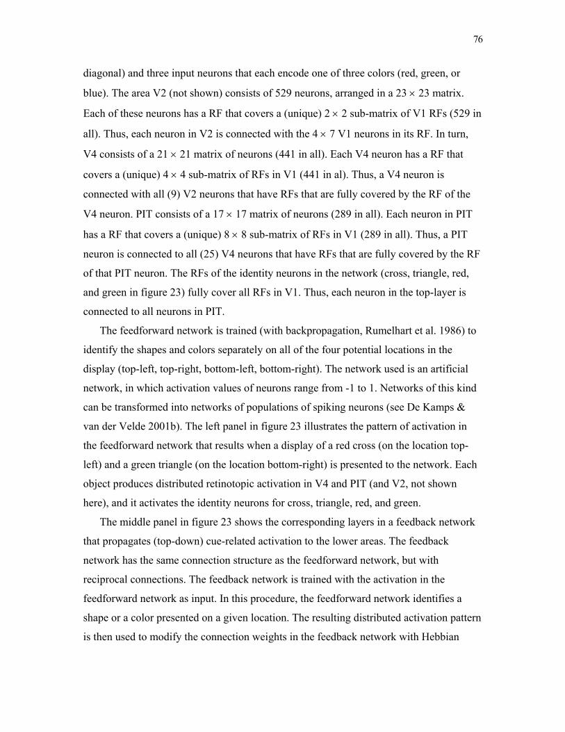
76
diagonal) and three input neurons that each encode one of three colors (red, green, or
blue). The area V2 (not shown) consists of 529 neurons, arranged in a 23 × 23 matrix.
Each of these neurons has a RF that covers a (unique) 2 × 2 sub-matrix of V1 RFs (529 in
all). Thus, each neuron in V2 is connected with the 4 × 7 V1 neurons in its RF. In turn,
V4 consists of a 21 × 21 matrix of neurons (441 in all). Each V4 neuron has a RF that
covers a (unique) 4 × 4 sub-matrix of RFs in V1 (441 in al). Thus, a V4 neuron is
connected with all (9) V2 neurons that have RFs that are fully covered by the RF of the
V4 neuron. PIT consists of a 17 × 17 matrix of neurons (289 in all). Each neuron in PIT
has a RF that covers a (unique) 8 × 8 sub-matrix of RFs in V1 (289 in all). Thus, a PIT
neuron is connected to all (25) V4 neurons that have RFs that are fully covered by the RF
of that PIT neuron. The RFs of the identity neurons in the network (cross, triangle, red,
and green in figure 23) fully cover all RFs in V1. Thus, each neuron in the top-layer is
connected to all neurons in PIT.
The feedforward network is trained (with backpropagation, Rumelhart et al. 1986) to
identify the shapes and colors separately on all of the four potential locations in the
display (top-left, top-right, bottom-left, bottom-right). The network used is an artificial
network, in which activation values of neurons range from -1 to 1. Networks of this kind
can be transformed into networks of populations of spiking neurons (see De Kamps &
van der Velde 2001b). The left panel in figure 23 illustrates the pattern of activation in
the feedforward network that results when a display of a red cross (on the location top-
left) and a green triangle (on the location bottom-right) is presented to the network. Each
object produces distributed retinotopic activation in V4 and PIT (and V2, not shown
here), and it activates the identity neurons for cross, triangle, red, and green.
The middle panel in figure 23 shows the corresponding layers in a feedback network
that propagates (top-down) cue-related activation to the lower areas. The feedback
network has the same connection structure as the feedforward network, but with
reciprocal connections. The feedback network is trained with the activation in the
feedforward network as input. In this procedure, the feedforward network identifies a
shape or a color presented on a given location. The resulting distributed activation pattern
is then used to modify the connection weights in the feedback network with Hebbian
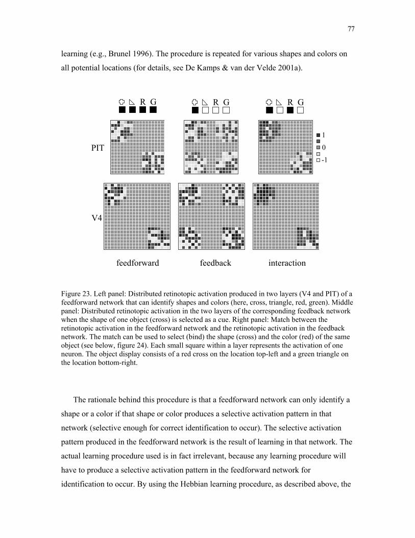
77
learning (e.g., Brunel 1996). The procedure is repeated for various shapes and colors on
all potential locations (for details, see De Kamps & van der Velde 2001a).
Figure 23. Left panel: Distributed retinotopic activation produced in two layers (V4 and PIT) of a feedforward network that can identify shapes and colors (here, cross, triangle, red, green). Middle panel: Distributed retinotopic activation in the two layers of the corresponding feedback network when the shape of one object (cross) is selected as a cue. Right panel: Match between the retinotopic activation in the feedforward network and the retinotopic activation in the feedback network. The match can be used to select (bind) the shape (cross) and the color (red) of the same object (see below, figure 24). Each small square within a layer represents the activation of one neuron. The object display consists of a red cross on the location top-left and a green triangle on the location bottom-right.
The rationale behind this procedure is that a feedforward network can only identify a
shape or a color if that shape or color produces a selective activation pattern in that
network (selective enough for correct identification to occur). The selective activation
pattern produced in the feedforward network is the result of learning in that network. The
actual learning procedure used is in fact irrelevant, because any learning procedure will
have to produce a selective activation pattern in the feedforward network for
identification to occur. By using the Hebbian learning procedure, as described above, the
1
-1
0
R G R G R G
feedforward feedback interaction
PIT
V4
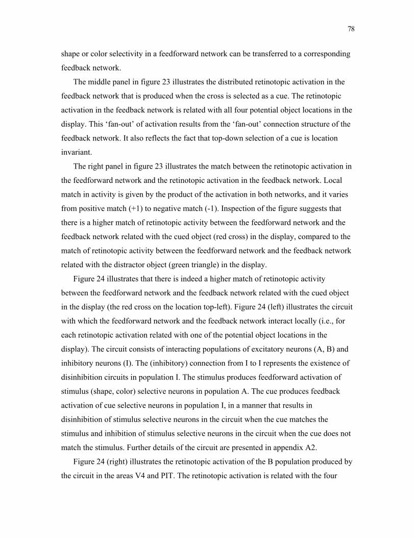
78
shape or color selectivity in a feedforward network can be transferred to a corresponding
feedback network.
The middle panel in figure 23 illustrates the distributed retinotopic activation in the
feedback network that is produced when the cross is selected as a cue. The retinotopic
activation in the feedback network is related with all four potential object locations in the
display. This ‘fan-out’ of activation results from the ‘fan-out’ connection structure of the
feedback network. It also reflects the fact that top-down selection of a cue is location
invariant.
The right panel in figure 23 illustrates the match between the retinotopic activation in
the feedforward network and the retinotopic activation in the feedback network. Local
match in activity is given by the product of the activation in both networks, and it varies
from positive match (+1) to negative match (-1). Inspection of the figure suggests that
there is a higher match of retinotopic activity between the feedforward network and the
feedback network related with the cued object (red cross) in the display, compared to the
match of retinotopic activity between the feedforward network and the feedback network
related with the distractor object (green triangle) in the display.
Figure 24 illustrates that there is indeed a higher match of retinotopic activity
between the feedforward network and the feedback network related with the cued object
in the display (the red cross on the location top-left). Figure 24 (left) illustrates the circuit
with which the feedforward network and the feedback network interact locally (i.e., for
each retinotopic activation related with one of the potential object locations in the
display). The circuit consists of interacting populations of excitatory neurons (A, B) and
inhibitory neurons (I). The (inhibitory) connection from I to I represents the existence of
disinhibition circuits in population I. The stimulus produces feedforward activation of
stimulus (shape, color) selective neurons in population A. The cue produces feedback
activation of cue selective neurons in population I, in a manner that results in
disinhibition of stimulus selective neurons in the circuit when the cue matches the
stimulus and inhibition of stimulus selective neurons in the circuit when the cue does not
match the stimulus. Further details of the circuit are presented in appendix A2.
Figure 24 (right) illustrates the retinotopic activation of the B population produced by
the circuit in the areas V4 and PIT. The retinotopic activation is related with the four
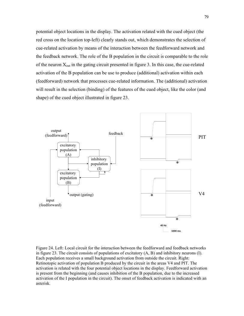
79
potential object locations in the display. The activation related with the cued object (the
red cross on the location top-left) clearly stands out, which demonstrates the selection of
cue-related activation by means of the interaction between the feedforward network and
the feedback network. The role of the B population in the circuit is comparable to the role
of the neuron Xout in the gating circuit presented in figure 3. In this case, the cue-related
activation of the B population can be use to produce (additional) activation within each
(feedforward) network that processes cue-related information. The (additional) activation
will result in the selection (binding) of the features of the cued object, like the color (and
shape) of the cued object illustrated in figure 23.
Figure 24. Left: Local circuit for the interaction between the feedforward and feedback networks in figure 23. The circuit consists of populations of excitatory (A, B) and inhibitory neurons (I). Each population receives a small background activation from outside the circuit. Right: Retinotopic activation of population B produced by the circuit in the areas V4 and PIT. The activation is related with the four potential object locations in the display. Feedforward activation is present from the beginning (and causes inhibition of the B population, due to the increased activation of the I population in the circuit). The onset of feedback activation is indicated with an asterisk.
excitatory population
(A)
excitatory population
(B)
inhibitory population
(I)
output (gating)input
(feedforward)
feedbackoutput
(feedforward)
40 Hz
1000 ms
V4
PIT*
*
*
*
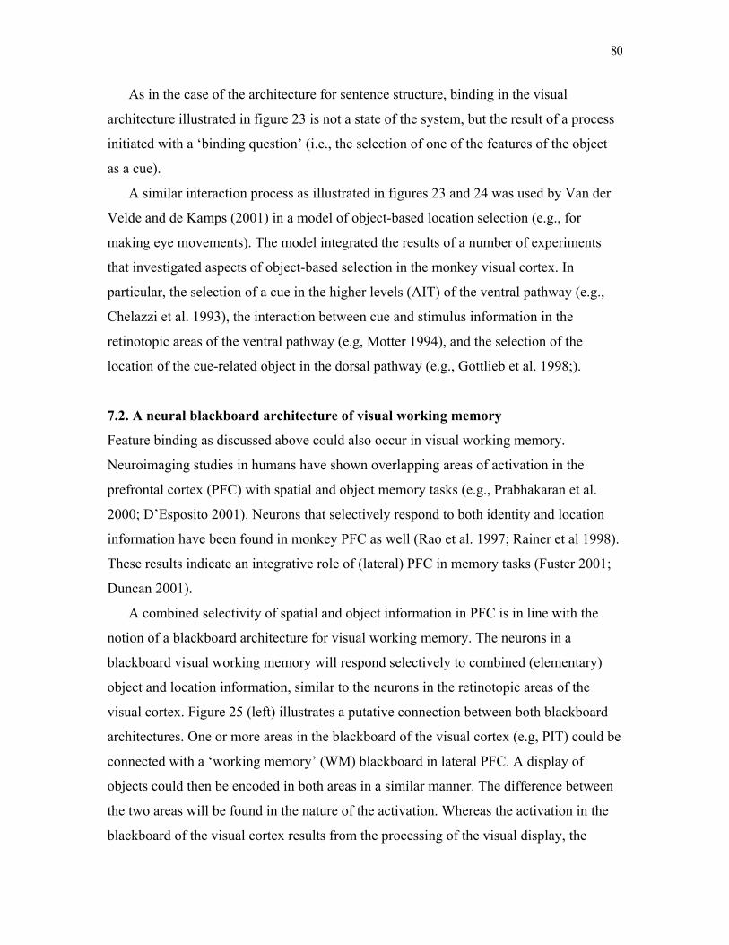
80
As in the case of the architecture for sentence structure, binding in the visual
architecture illustrated in figure 23 is not a state of the system, but the result of a process
initiated with a ‘binding question’ (i.e., the selection of one of the features of the object
as a cue).
A similar interaction process as illustrated in figures 23 and 24 was used by Van der
Velde and de Kamps (2001) in a model of object-based location selection (e.g., for
making eye movements). The model integrated the results of a number of experiments
that investigated aspects of object-based selection in the monkey visual cortex. In
particular, the selection of a cue in the higher levels (AIT) of the ventral pathway (e.g.,
Chelazzi et al. 1993), the interaction between cue and stimulus information in the
retinotopic areas of the ventral pathway (e.g, Motter 1994), and the selection of the
location of the cue-related object in the dorsal pathway (e.g., Gottlieb et al. 1998;).
7.2. A neural blackboard architecture of visual working memory
Feature binding as discussed above could also occur in visual working memory.
Neuroimaging studies in humans have shown overlapping areas of activation in the
prefrontal cortex (PFC) with spatial and object memory tasks (e.g., Prabhakaran et al.
2000; D’Esposito 2001). Neurons that selectively respond to both identity and location
information have been found in monkey PFC as well (Rao et al. 1997; Rainer et al 1998).
These results indicate an integrative role of (lateral) PFC in memory tasks (Fuster 2001;
Duncan 2001).
A combined selectivity of spatial and object information in PFC is in line with the
notion of a blackboard architecture for visual working memory. The neurons in a
blackboard visual working memory will respond selectively to combined (elementary)
object and location information, similar to the neurons in the retinotopic areas of the
visual cortex. Figure 25 (left) illustrates a putative connection between both blackboard
architectures. One or more areas in the blackboard of the visual cortex (e.g, PIT) could be
connected with a ‘working memory’ (WM) blackboard in lateral PFC. A display of
objects could then be encoded in both areas in a similar manner. The difference between
the two areas will be found in the nature of the activation. Whereas the activation in the
blackboard of the visual cortex results from the processing of the visual display, the
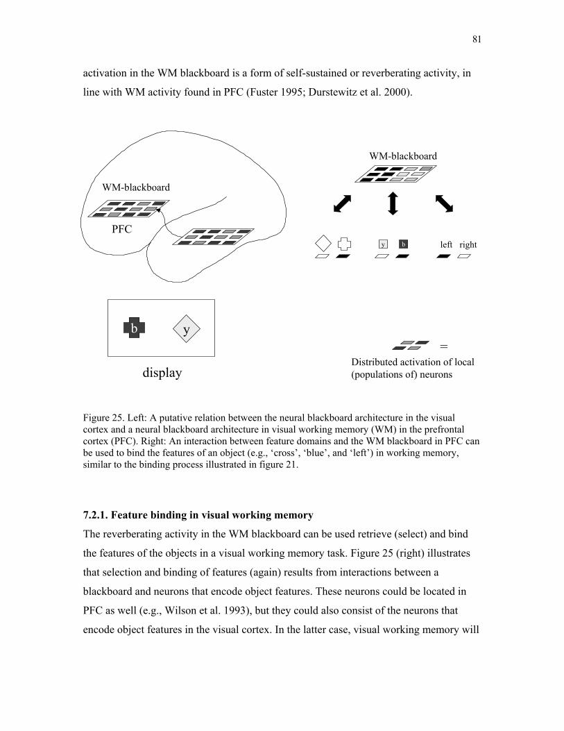
81
activation in the WM blackboard is a form of self-sustained or reverberating activity, in
line with WM activity found in PFC (Fuster 1995; Durstewitz et al. 2000).
Figure 25. Left: A putative relation between the neural blackboard architecture in the visual cortex and a neural blackboard architecture in visual working memory (WM) in the prefrontal cortex (PFC). Right: An interaction between feature domains and the WM blackboard in PFC can be used to bind the features of an object (e.g., ‘cross’, ‘blue’, and ‘left’) in working memory, similar to the binding process illustrated in figure 21.
7.2.1. Feature binding in visual working memory
The reverberating activity in the WM blackboard can be used retrieve (select) and bind
the features of the objects in a visual working memory task. Figure 25 (right) illustrates
that selection and binding of features (again) results from interactions between a
blackboard and neurons that encode object features. These neurons could be located in
PFC as well (e.g., Wilson et al. 1993), but they could also consist of the neurons that
encode object features in the visual cortex. In the latter case, visual working memory will
WM-blackboard
PFCleft right
WM-blackboard
y b
b y
displayDistributed activation of local (populations of) neurons
=
82
consist of interactions between neurons in PFC and neurons in posterior visual areas
(Ruchlin et al. in press).
The nature of the WM blackboard produces the behavioral effects reported by Luck
& Vogel (1997). They observed that the number of objects that can be maintained in
working memory is limited, but the number of their features is not. In terms of the WM
blackboard, too many objects in a display will cause an interference between their
distributed activations in the WM blackboard. This interference results in a limitation of
the number of objects that can be maintained in working memory, as simulated by Van
der Voort van der Kleij et al. (2003). However, the number of features for each object is
not limited. That is, all features of an object can be selected by means of the interaction
with the blackboard (figure 25, right) as long as the object activations in the WM
blackboard do not interfere.
7.3. Feature binding in long-term memory
Feature binding in visual working memory, as described above, is instantiated in terms of
the sustained activation in the WM blackboard. As discussed in section 2.4, this raises the
question of how feature binding can be achieved in terms of synaptic modification, which
forms the basis of long-term memory. In the case of linguistic structures, this question
was answered in terms of the process illustrated in figure 11. The answer proceeds along
similar lines for visual feature binding.
Figure 26 (left) illustrates the role of the HC in the case of visual features. A neuron
in the HC forms a conjunctive encoding of the object features that are activated by a
display of two objects (a blue cross on the left and a yellow diamond on the right). In this
way, the neurons that encode the object features can be reactivated when the neuron in
the HC is reactivated. However, it is clear that the conjunctive encoding by the HC
neuron results in the familiar binding problem (Von der Malsburg 1987), because the
relations between the object features are lost in this form of encoding. A display of, say, a
yellow cross and a blue diamond (on any of the two locations) would activate the same
object features, and would thus be encoded in the same way by the HC neuron as the
display in figure 26.
83
Figure 26. Left: Conjunctive encoding of the object features (e.g., shape, color, location) of two objects with a neuron (or group of neurons) in the hippocampus complex (HC). Right: Conjunctive encoding of the object features and a neural blackboard with a neuron (or group of neurons) in the hippocampus complex (HC).
However, as in figure 11, the relations between the object features can be encoded by
the HC neurons, if a neural blackboard (e.g., the WM blackboard) is included in the
conjunctive encoding, as illustrated in figure 26 (right). In this case, the relationship
information is part of the input to the HC (as described by O'Reilly & Rudy 2001), so that
the HC can encode the relationship information (the blackboard) together with the object
features. When the HC neurons reactivate the blackboard and the object features, the
relations between the features of the objects in the display can be retrieved in the manner
illustrated in figure 25. The encoding of different events (episodes) in this architecture
can proceed in a manner similar to the process illustrated in figure 12.
Figure 26 illustrates again how a blackboard architecture can be play an important
y b left right
HCHC
y b left right
location shape color
blackboard
b y
displayDistributed activation of local (populations of) neurons
=
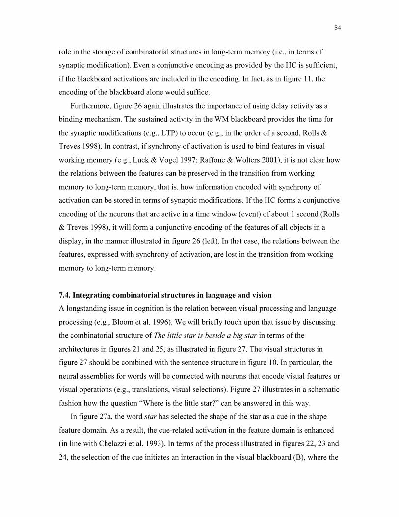
84
role in the storage of combinatorial structures in long-term memory (i.e., in terms of
synaptic modification). Even a conjunctive encoding as provided by the HC is sufficient,
if the blackboard activations are included in the encoding. In fact, as in figure 11, the
encoding of the blackboard alone would suffice.
Furthermore, figure 26 again illustrates the importance of using delay activity as a
binding mechanism. The sustained activity in the WM blackboard provides the time for
the synaptic modifications (e.g., LTP) to occur (e.g., in the order of a second, Rolls &
Treves 1998). In contrast, if synchrony of activation is used to bind features in visual
working memory (e.g., Luck & Vogel 1997; Raffone & Wolters 2001), it is not clear how
the relations between the features can be preserved in the transition from working
memory to long-term memory, that is, how information encoded with synchrony of
activation can be stored in terms of synaptic modifications. If the HC forms a conjunctive
encoding of the neurons that are active in a time window (event) of about 1 second (Rolls
& Treves 1998), it will form a conjunctive encoding of the features of all objects in a
display, in the manner illustrated in figure 26 (left). In that case, the relations between the
features, expressed with synchrony of activation, are lost in the transition from working
memory to long-term memory.
7.4. Integrating combinatorial structures in language and vision
A longstanding issue in cognition is the relation between visual processing and language
processing (e.g., Bloom et al. 1996). We will briefly touch upon that issue by discussing
the combinatorial structure of The little star is beside a big star in terms of the
architectures in figures 21 and 25, as illustrated in figure 27. The visual structures in
figure 27 should be combined with the sentence structure in figure 10. In particular, the
neural assemblies for words will be connected with neurons that encode visual features or
visual operations (e.g., translations, visual selections). Figure 27 illustrates in a schematic
fashion how the question “Where is the little star?” can be answered in this way.
In figure 27a, the word star has selected the shape of the star as a cue in the shape
feature domain. As a result, the cue-related activation in the feature domain is enhanced
(in line with Chelazzi et al. 1993). In terms of the process illustrated in figures 22, 23 and
24, the selection of the cue initiates an interaction in the visual blackboard (B), where the
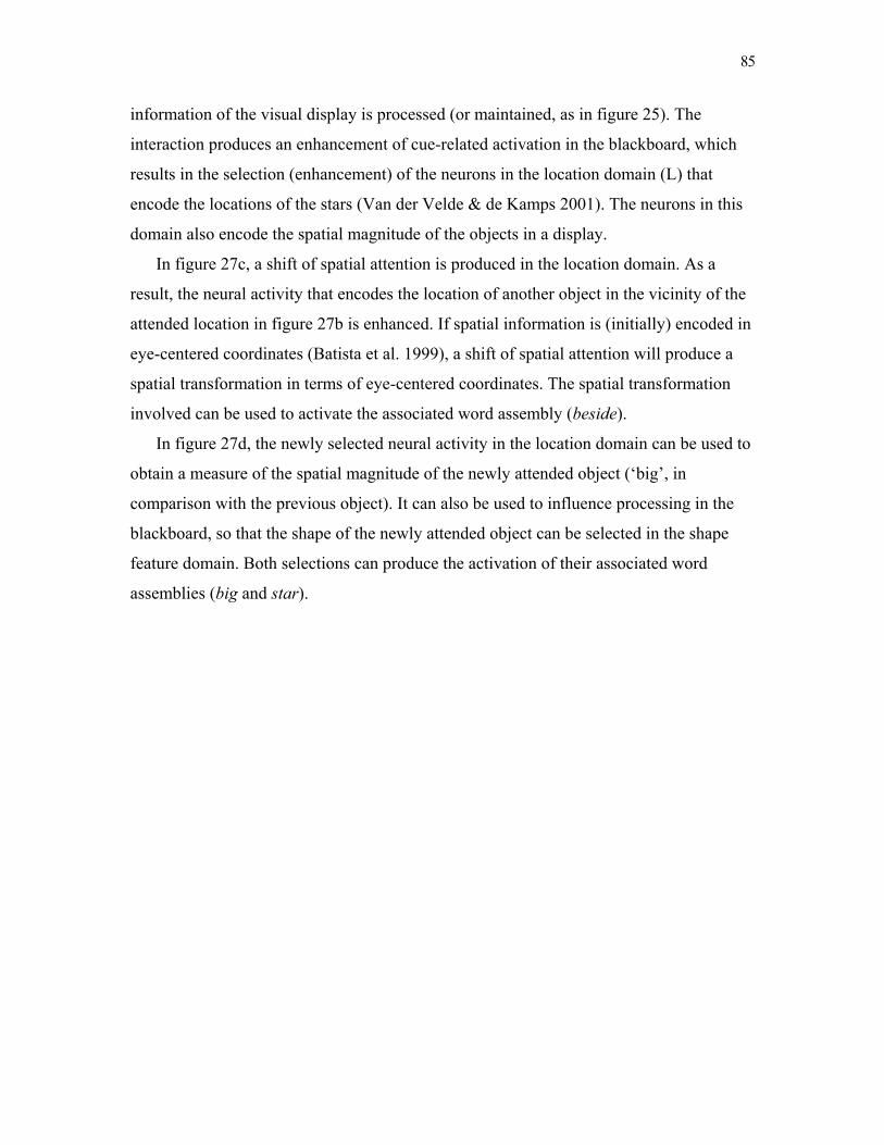
85
information of the visual display is processed (or maintained, as in figure 25). The
interaction produces an enhancement of cue-related activation in the blackboard, which
results in the selection (enhancement) of the neurons in the location domain (L) that
encode the locations of the stars (Van der Velde & de Kamps 2001). The neurons in this
domain also encode the spatial magnitude of the objects in a display.
In figure 27c, a shift of spatial attention is produced in the location domain. As a
result, the neural activity that encodes the location of another object in the vicinity of the
attended location in figure 27b is enhanced. If spatial information is (initially) encoded in
eye-centered coordinates (Batista et al. 1999), a shift of spatial attention will produce a
spatial transformation in terms of eye-centered coordinates. The spatial transformation
involved can be used to activate the associated word assembly (beside).
In figure 27d, the newly selected neural activity in the location domain can be used to
obtain a measure of the spatial magnitude of the newly attended object (‘big’, in
comparison with the previous object). It can also be used to influence processing in the
blackboard, so that the shape of the newly attended object can be selected in the shape
feature domain. Both selections can produce the activation of their associated word
assemblies (big and star).
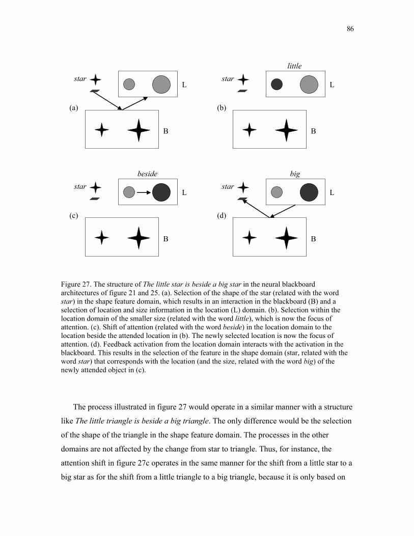
86
Figure 27. The structure of The little star is beside a big star in the neural blackboard architectures of figure 21 and 25. (a). Selection of the shape of the star (related with the word star) in the shape feature domain, which results in an interaction in the blackboard (B) and a selection of location and size information in the location (L) domain. (b). Selection within the location domain of the smaller size (related with the word little), which is now the focus of attention. (c). Shift of attention (related with the word beside) in the location domain to the location beside the attended location in (b). The newly selected location is now the focus of attention. (d). Feedback activation from the location domain interacts with the activation in the blackboard. This results in the selection of the feature in the shape domain (star, related with the word star) that corresponds with the location (and the size, related with the word big) of the newly attended object in (c).
The process illustrated in figure 27 would operate in a similar manner with a structure
like The little triangle is beside a big triangle. The only difference would be the selection
of the shape of the triangle in the shape feature domain. The processes in the other
domains are not affected by the change from star to triangle. Thus, for instance, the
attention shift in figure 27c operates in the same manner for the shift from a little star to a
big star as for the shift from a little triangle to a big triangle, because it is only based on
star
B
L
(a)
star
B
L
(b)
little
star
B
L
(c)
besidestar
B
L
(d)
big

87
the information in the location domain. Likewise, in a structure like The little diamond is
above a big square, the process in figure 27a is only affected by the (initial) selection of
the shape of the diamond (instead of the star or the triangle), and the process in figure 27c
is only affected by the nature of the spatial transformation (above, instead of beside).
The similarity between these examples emphasizes the combinatorial nature of the
process illustrated in figure 27. Each of the individual processes operates only on
information that is available in its own domain. However, by using the blackboard, a
process in one domain can influence the processes in the other domains. In this way, a
combinatorial structure can be produced by the architecture as a whole. For instance, with
The little diamond is above a big square, the attention shift in figure 27c will produce the
square as the second object selected in the shape feature domain (instead of the star or the
triangle in the other examples), by the interaction process in the blackboard illustrated in
figure 27d.
7.5. Related issues
The architecture for combinatorial structures in vision discussed here is related with a
number of issues that we can only briefly mention. The interactions between object
(feature) information and spatial information, illustrated in figure 27, have a clear relation
with attentional processes in the cortex (e.g., as in the ‘bias competition’ model of
attention, Desimone & Duncan 1995). The blackboard architecture in the visual cortex
(figure 21) and the blackboard architecture of visual working memory (figure 25) can be
combined in a ‘closed-loop attention model’ (Van der Velde et al. 2004b). Another issue
is the question of how and to what extent the architectures for combinatorial structures
discussed here are related to processing of object identification (e.g., Biederman 1987;
Edelman & Intrator 2003). Finally, the interaction between neural sentence structures
(figure 10) and visual blackboard structures, as illustrated in figure 27, could also form
the basis of a model that combines pictorial and propositional aspects of mental imagery
(for a discussion on that topic see Pylyshyn 2002, Van der Velde and de Kamps 2002b).

88
8. Conclusion and perspective
The aim of our paper is to show that the problems described by Jackendoff (2002) can be
solved by means of neural blackboard architectures. To this end, we have discussed and
illustrated how two kinds of combinatorial structures (linguistic and visual) can be
instantiated in terms of neural blackboard architectures. As can be expected, there are
clear structural differences between these architectures, which derive from the nature of
the information processing in which they are involved (in this case, the spatial
arrangement of visual features in a visual display versus the sequential arrangement of
words in a sentence). However, there are also important similarities between the different
blackboard architectures.
One similarity concerns the solution for the binding problem in each architecture. In
both architectures, the binding problem is solved in terms of a process that answers
specific ‘binding questions’ related to the binding at hand. This process consists of a
selective flow of activation. Thus, the binding of features in the visual blackboard
architectures consists of a selective flow of activation from one feature domain to
another, determined by the interaction process in the blackboard. Likewise, the
blackboard architecture for sentence structure produces a selective flow of activation in
the process of answering a ‘binding’ question.
Another similarity between the architectures concerns the transition from working
memory to long-term memory, and the role of delay activity as a binding mechanism.
Combinatorial structures can be stored in long-term memory (using synaptic
modification) when the blackboard activity is included in a conjunctive form of encoding
as provided by the hippocampus complex. The delay activity in the blackboard provides
the time for the synaptic modifications (Hebbian learning) to occur, even in the case of
one-trial learning.
We also discussed and illustrated the potential for further development of the
architectures we presented. It is clear that a substantial amount of work is needed to fulfill
this potential. However, concerning the problems he discussed, Jackendoff (2002, p. 64)
noted that “some further technical innovation is called for in neural network models …
upon the development of such an innovation, the dialogue between linguistic theory and
neural network modelling will begin to be more productive”. The examples of the neural
89
sentence structures we discussed illustrate how such a dialogue could proceed.
We would argue that this technical innovation is also needed for the development of
cognitive neuroscience models. In the preface of “The Cognitive Neurosciences”,
Gazzaniga (1995, p. xiii) described the aim of cognitive neuroscience as follows: “At
some point in the future, cognitive neuroscience will be able to describe the algorithms
that drive structural neural elements into the physiological activity that results in
perception, cognition, and perhaps even consciousness. To reach this goal, the field has
departed from the more limited aims of neuropsychology and basic neuroscience. Simple
descriptions of clinical disorders are a beginning, as is understanding basic mechanisms
of neural action. The future of the field, however, is in working toward a science that
truly relates brain and cognition in a mechanistic way.”
If the ultimate aim of cognitive neuroscience is to deliver detailed neural models of
cognitive processes, the question arises how such models can be developed and tested17.
In some cases, like visual processing, an animal model exists that can be studied with the
kind of experiments described in section 7.1.2. But for language and other aspects of
high-level human cognition an animal model is missing, which excludes the kind of
rigorous investigation of neural activity on a cell level that is possible with visual
processing. In figure 8, we presented the neural activity of some of the assemblies
presented in figure 7a. As the lines and labels in figure 7a suggest, one can see the
activity presented in figure 8 as the result of virtual electrodes inserted in the model. In a
similar way, one could compare the model with observations made with real electrodes,
except for the considerations that prevent such a testing. On the other hand, neuroimaging
methods like EEG and fMRI provide rather coarse observations of neural activity, not
(yet) on the level of the detailed neural mechanisms needed to relate brain and cognition
in a mechanistic way.
If the aim of cognitive neuroscience is to relate brain and cognition in a mechanistic
way, then the gap that seems to exist between detailed neural mechanisms and the current
methods of observation is a problem for both modelling and neuroimaging18. In our view,
the best way to close this gap is the integration of modelling and neuroimaging that we
described in section 6.9. In short, on the basis of detailed models, activation processes
can be derived that can be compared with neuroimaging observations. In turn, these
90
observations can be used to modify or change the existing models. This process is
technically demanding and can only proceed in a step by step manner, but it may be the
only way to fulfil the aim of cognitive neuroscience as described by Gazzaniga.
However, the success of this process depends on further advances in both
neuroimaging and modelling. In neuroimaging, further development of techniques like
dynamic causal modelling (e.g., Friston et al. 2003) and further integration of EEG and
fMRI is needed. In modelling, neural models are needed that can capture important
aspects of human cognition, such as the productivity and systematicity that derives from
the ability to process combinatorial structures.
Thus, it is clear that a substantial amount of work, both theoretically and empirically,
is needed to develop an understanding of the neural basis of combinatorial structures in
human cognition. However, the similarities between the potential neural instantiation of
combinatorial sentence structures and the (more familiar) neural instantiation of
combinatorial structures in visual cognition as described here provide the hope that such
a development can be successful in the near future.
Notes
1. Tensor networks could perhaps be included here. However, tensor networks fail to
instantiate combinatorial structures (Fodor and McLaughlin, 1990). Basically, this results
from the fact that a tensor is just a list of constituents, organized in a particular fashion
(i.e., as a n-dimensional list for a rank-n tensor). Any operation on a tensor consists of
selecting a k-dimensional subset of the constituents in the tensor (with k ≤ n). But all
selected subsets have to be listed in the tensor beforehand, which limits the instantiation
of novel structures. Furthermore, adding constituents to the tensor increases the
dimensions of the tensor, which requires adjustments to all components in the cognitive
system that can interact with the tensor.
2. The sentence presented by Jackendoff (2002) is The little star's beside a big star, with
the clitic z ('s) to emphasize the phonological structure of the sentence. Phonological

91
structure is not discussed here, therefore the clitic z is omitted.
3. When a symbol is copied and moved elsewhere, it is detached from its network of
relations and associations. One could try to reestablish these relations and associations
from time to time, but this requires an active process, executed by a control structure.
Active control would be needed constantly, to decide how many of these relations and
associations have to be reestablished (and how often).
4. Pilot simulations showed that RNNs are very good at reproducing learned word-word
associations. Thus, with the test sentence boy hears girl, we wanted to avoid
combinations like boy hears and hears girl in the training sentences. Other than that, we
wanted to train as much relations between these words as possible. In the case of this test
sentence, the RNNs learned the relation boy Verb girl. Furthermore, they learned the
relation dog Verb girl with dog hears Noun, and the relation boy Verb cat with Noun
hears cat.
5. We are not aware of pathological behavior of this kind. Broca's aphasics, for instance,
often fail on sentences like girl who dog hears obeys Mary, but they can still understand
sentences like boy hears girl (Grodzinsky 2000).
6. Verbs can have one, two, or three arguments, or thematic roles. Although in semantic
terms many different kinds of arguments can be distinguished, they can be grouped into
‘semantic macroroles’(Van Valin 2001). We will refer to these as ‘agent’, ‘theme’, and
(later on) ‘recipient’.
7. When a NP assembly is bound to a sentence structure, at least one of its memory
circuits is active. This activation can be used as a signal that the NP assembly is not free.
Or, one could have an ‘inhibition of return’ that prevents the reactivation of a structure
assembly activated recently.
8. The inhibition of the active NP assembly could result from initiating a competition
92
between the NP assemblies. Due to its high transient activity, frequently found with a
new stimulus, the new NP assembly could win the competition. Or, the occurrence of a
new noun could result in the inhibition of the active NP assembly before a new NP
assembly is generated.
9. The delay assemblies produce inhibition by activating inhibitory interneurons.
10. If tree-like structures capture important aspects of sentence structures, neural
instantiations of sentence structures can always be transformed into tree-like structures.
This is a direct consequence of having a neural instantiation of a sentence structure. It can
be compared with the gradual transformation of one computer language into another. It is
a matter of choice which of the intermediary structures are used to illustrate the
transformation. A comparison of figures 7 and 7a shows that it is more useful to discuss
the architecture in terms of the structures illustrated in figure 7 than those in figure 7a.
Yet, both figures represent the same architecture, and can be transformed into one
another.
11. In linguistics, words are the terminal notes placed at the bottom of a sentence
structure. Here, they are placed close to their structure assemblies.
12. The structures in figures 11 (left) and 1 (bottom) are not the same. Figure 11 (left)
represents a conjunctive encoding that results from direct associations between each of
the word assemblies and the HC neuron. In figure 1 (bottom), a specific neural circuit
will activate a ‘sentence’ neuron, when the word assemblies have been activated in the
correct order. Circuits of this kind are much harder to develop than the conjunctive
encoding in figure 11.
13. Transitions from an attractor state into an associated attractor state have been
observed in the cortex (Yakovlev et al., 1998).
14. A difference could be found in clause-based closure principles (e.g., see Gibson
93
1998). For instance, a relative clause can be closed without closing a matrix clause, but a
matrix clause cannot be closed without closing a relative clause.
15. The connection structure illustrated in figure 19 was not specifically designed to
operate as a pushdown stack. Instead, it was designed to satisfy two constraints. First, the
constraint of combinatorial productivity, which entails that every A subassembly should
be able to bind with every B subassembly (and vice versa). This constraint is satisfied
with the matrix-like array of columns in the connection structure. Second, the uniqueness
constraint, which entails that a given A subassembly can only bind with one B
subassembly (and vice versa). This constraint is satisfied with the inhibition within the
horizontal and vertical rows of columns. The resulting connection structure operates as a
pushdown stack if the reverberating activity in the structure decays over time.
16. The image of a purple cow is used in an advertisement campaign of a brand of milk
chocolate bars, sold in a purple wrap.
17. Perhaps we do not need to study the neural instantiation of cognition. In the view of
‘classical’ cognitive psychology (e.g., Fodor & Pylyshyn 1988), implementation is
irrelevant for the nature of a computational model of a cognitive process. A mathematical
critique of this position can be found in Van der Velde (2001). Here, we point out that
Fodor (2000) has argued that the computational theory of mind is incomplete, in fact only
a fraction of the truth. If so, it makes even more sense to study how computational
processes can be implemented in the brain. We know that the brain produces cognition (it
is the only example we are certain of). So, if we have an idea of how computational
processes could be matched onto brain processes, we could also get a clearer view of
what could be missing in the computational account.
18. An alternative would be to reformulate the aim of cognitive neuroscience. Or, what
amounts to the same thing, to abandon cognitive neuroscience as described by Gazzaniga.
We do not advocate such a position.
94
References
Amit, D. (1989) Modeling brain function. Cambridge University Press.
Anderson, J. R. (1983) The architecture of cognition. Cambridge, MA: Harvard
University Press.
Barsalou, L. W. (1999) Perceptual symbol systems. Behavioral and Brain Sciences
22:577-660.
Barsalou, L. W., Simmons, W. K., Barbey, A. K. & Wilson, C. D. (2003) Grounding
conceptual knowledge in modality-specific systems. Trends in Cognitive Sciences 7:84-
91.
Batista, A. P., Buneo, C. A. Snyder, L. H. & Andersen, R. A. (1999) Reach plans in eye-
centered coordinates. Science 285:257-260.
Bechtel, W. & Abrahamsen, A. (2002) Connectionism and the mind. Malden, MA:
Blackwell.
Ben-Sachar, M., Hendler, T., Kahn, I., Ben-Bashat, D. & Grodzinsky, Y. (2003) The
neural reality of syntactic transformations: Evidence from functional magnetic resonance
imaging. Psychological Science, 14:433-440.
Biederman, I. (1987) Recognition by components: A theory of human image
understanding. Psychological Review 94:115-147.
Bierwisch, M. (1999) Words in the brain are not just labeled concepts. Behavioral and
Brain Sciences 22:280-282.
Bloom, P. (2000) How children learn the meanings of words. Cambridge, MA: MIT
Press.
Bloom, P., Peterson, M. A., Nadel, L & Garrett, M. F., eds (1996). Language and space.
Cambridge, MA: MIT Press.
Brunel, N. (1996) Hebbian learning of context in recurrent neural networks. Neural
Computation 8:1677-1710.
Bulier J. (2001) Feedback connections and conscious vision. Trends in Cognitive
Sciences 5:369-370.
Calvin, W. H. & Bickerton, D. (2000) Lingua ex machina: Reconciling Darwin and
Chomsky with the human brain. Cambridge, MA: MIT Press.
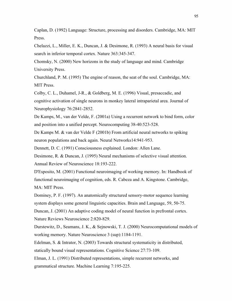
95
Caplan, D. (1992) Language: Structure, processing and disorders. Cambridge, MA: MIT
Press.
Chelazzi, L., Miller, E. K., Duncan, J. & Desimone, R. (1993) A neural basis for visual
search in inferior temporal cortex. Nature 363:345-347.
Chomsky, N. (2000) New horizons in the study of language and mind. Cambridge
University Press.
Churchland, P. M. (1995) The engine of reason, the seat of the soul. Cambridge, MA:
MIT Press.
Colby, C. L., Duhamel, J-R., & Goldberg, M. E. (1996) Visual, presaccadic, and
cognitive activation of single neurons in monkey lateral intraparietal area. Journal of
Neurophysiology 76:2841-2852.
De Kamps, M., van der Velde, F. (2001a) Using a recurrent network to bind form, color
and position into a unified percept. Neurocomputing 38-40:523-528.
De Kamps M. & van der Velde F (2001b) From artificial neural networks to spiking
neuron populations and back again. Neural Networks14:941-953.
Dennett, D. C. (1991) Consciousness explained. London: Allen Lane.
Desimone, R. & Duncan, J. (1995) Neural mechanisms of selective visual attention.
Annual Review of Neuroscience 18:193-222.
D'Esposito, M. (2001) Functional neuroimaging of working memory. In: Handbook of
functional neuroimaging of cognition, eds. R. Cabeza and A. Kingstone. Cambridge,
MA: MIT Press.
Dominey, P. F. (1997). An anatomically structured sensory-motor sequence learning
system displays some general linguistic capacities. Brain and Language, 59, 50-75.
Duncan, J. (2001) An adaptive coding model of neural function in prefrontal cortex.
Nature Reviews Neuroscience 2:820-829.
Durstewitz, D., Seamans, J. K., & Sejnowski, T. J. (2000) Neurocomputational models of
working memory. Nature Neuroscience 3 (sup):1184-1191.
Edelman, S. & Intrator, N. (2003) Towards structural systematicity in distributed,
statically bound visual representations. Cognitive Science 27:73-109.
Elman, J. L. (1991) Distributed representations, simple recurrent networks, and
grammatical structure. Machine Learning 7:195-225.
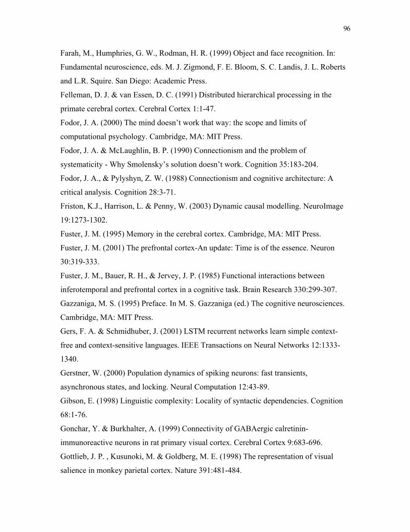
96
Farah, M., Humphries, G. W., Rodman, H. R. (1999) Object and face recognition. In:
Fundamental neuroscience, eds. M. J. Zigmond, F. E. Bloom, S. C. Landis, J. L. Roberts
and L.R. Squire. San Diego: Academic Press.
Felleman, D. J. & van Essen, D. C. (1991) Distributed hierarchical processing in the
primate cerebral cortex. Cerebral Cortex 1:1-47.
Fodor, J. A. (2000) The mind doesn’t work that way: the scope and limits of
computational psychology. Cambridge, MA: MIT Press.
Fodor, J. A. & McLaughlin, B. P. (1990) Connectionism and the problem of
systematicity - Why Smolensky’s solution doesn’t work. Cognition 35:183-204.
Fodor, J. A., & Pylyshyn, Z. W. (1988) Connectionism and cognitive architecture: A
critical analysis. Cognition 28:3-71.
Friston, K.J., Harrison, L. & Penny, W. (2003) Dynamic causal modelling. NeuroImage
19:1273-1302.
Fuster, J. M. (1995) Memory in the cerebral cortex. Cambridge, MA: MIT Press.
Fuster, J. M. (2001) The prefrontal cortex-An update: Time is of the essence. Neuron
30:319-333.
Fuster, J. M., Bauer, R. H., & Jervey, J. P. (1985) Functional interactions between
inferotemporal and prefrontal cortex in a cognitive task. Brain Research 330:299-307.
Gazzaniga, M. S. (1995) Preface. In M. S. Gazzaniga (ed.) The cognitive neurosciences.
Cambridge, MA: MIT Press.
Gers, F. A. & Schmidhuber, J. (2001) LSTM recurrent networks learn simple context-
free and context-sensitive languages. IEEE Transactions on Neural Networks 12:1333-
1340.
Gerstner, W. (2000) Population dynamics of spiking neurons: fast transients,
asynchronous states, and locking. Neural Computation 12:43-89.
Gibson, E. (1998) Linguistic complexity: Locality of syntactic dependencies. Cognition
68:1-76.
Gonchar, Y. & Burkhalter, A. (1999) Connectivity of GABAergic calretinin-
immunoreactive neurons in rat primary visual cortex. Cerebral Cortex 9:683-696.
Gottlieb, J. P. , Kusunoki, M. & Goldberg, M. E. (1998) The representation of visual
salience in monkey parietal cortex. Nature 391:481-484.

97
Grodzinsky, Y. (2000) The neurology of syntax: Language use without Broca’s area.
Behavioral and Brain Sciences 23:1-71.
Harnad, S. (1991) The symbol grounding problem. In: Emergent computation: Self-
organizing, collective, and cooperative phenomena in natural and artificial computing
networks, ed. S. Forrest. Cambridge, MA: MIT Press.
Hawkins, J. A. (1994) A performance theory of order and constituency. Cambridge
University Press.
Hebb, D. O. (1949) The organisation of behaviour. New York: Wiley.
Hubel, D. (1995) Eye, brain, and vision. New York: Scientific American Library.
Hummel, J. E. & Holyoak, K. J. (1993) Distributing structure over time. Behavioral and
Brain Sciences. 16:464.
Jackendoff, R. (2002) Foundations of language. Oxford: Oxford University Press.
Jackendoff, R. (in press) Précis to Foundations of language. Behavioral and Brain
Sciences.
Kling, U. and Szekély, G. (1968) Simulation of rhythmic activities. I. Function of
network with cyclic inhibitions. Kybernetics. 5: 89-103.
Koch, C. (1999). Biophysics of Computation: Information Processing in Single Neurons.
Oxford: Oxford University Press.
Koutsofios E & North, S. C. (1996) Drawing Graphs with dot.
http://research.att.com in dist/drawdag/dotguide.ps.Z.
Lewis, R. L. (1999) Accounting for the fine structure of syntactic working memory:
Similarity-based interference as a unifying principle. Behavioral and Brain Sciences
22:105-106.
Livingstone, M.S. & Hubel, D. H. (1988) Segregation of form, colour, movement and
depth: Anatomy, physiology, and perception. Science 240:740-749.
Luck, S. J. & Vogel, E. K. (1997) The capacity of visual working memory for features
and conjunctions. Nature 390:279-281.
Marcus, G. F. (2001) The algebraic mind. Cambridge, MA: MIT Press.
McClelland, J. L. & Kawamoto, A. H. (1986) Mechanisms of sentence processing:
Assigning roles to constituents. In: Parallel Distributed Processing: Explorations in the
Microstructure of Cognition, vol 2: Psychological and Biological Models, eds. J. L.
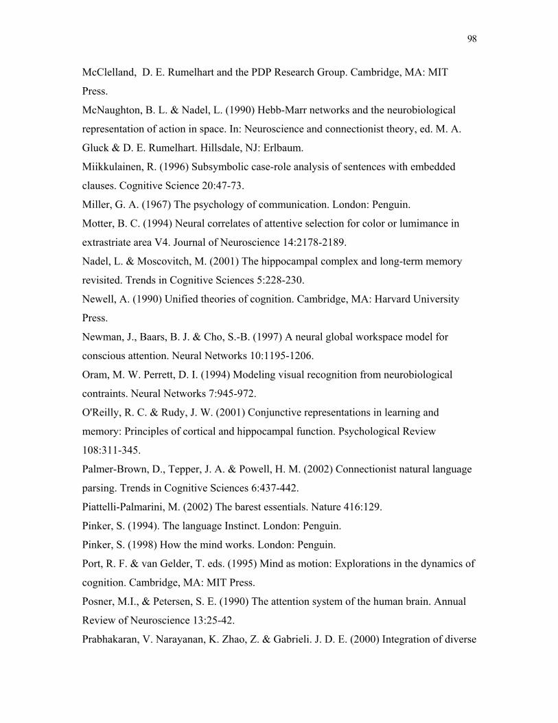
98
McClelland, D. E. Rumelhart and the PDP Research Group. Cambridge, MA: MIT
Press.
McNaughton, B. L. & Nadel, L. (1990) Hebb-Marr networks and the neurobiological
representation of action in space. In: Neuroscience and connectionist theory, ed. M. A.
Gluck & D. E. Rumelhart. Hillsdale, NJ: Erlbaum.
Miikkulainen, R. (1996) Subsymbolic case-role analysis of sentences with embedded
clauses. Cognitive Science 20:47-73.
Miller, G. A. (1967) The psychology of communication. London: Penguin.
Motter, B. C. (1994) Neural correlates of attentive selection for color or lumimance in
extrastriate area V4. Journal of Neuroscience 14:2178-2189.
Nadel, L. & Moscovitch, M. (2001) The hippocampal complex and long-term memory
revisited. Trends in Cognitive Sciences 5:228-230.
Newell, A. (1990) Unified theories of cognition. Cambridge, MA: Harvard University
Press.
Newman, J., Baars, B. J. & Cho, S.-B. (1997) A neural global workspace model for
conscious attention. Neural Networks 10:1195-1206.
Oram, M. W. Perrett, D. I. (1994) Modeling visual recognition from neurobiological
contraints. Neural Networks 7:945-972.
O'Reilly, R. C. & Rudy, J. W. (2001) Conjunctive representations in learning and
memory: Principles of cortical and hippocampal function. Psychological Review
108:311-345.
Palmer-Brown, D., Tepper, J. A. & Powell, H. M. (2002) Connectionist natural language
parsing. Trends in Cognitive Sciences 6:437-442.
Piattelli-Palmarini, M. (2002) The barest essentials. Nature 416:129.
Pinker, S. (1994). The language Instinct. London: Penguin.
Pinker, S. (1998) How the mind works. London: Penguin.
Port, R. F. & van Gelder, T. eds. (1995) Mind as motion: Explorations in the dynamics of
cognition. Cambridge, MA: MIT Press.
Posner, M.I., & Petersen, S. E. (1990) The attention system of the human brain. Annual
Review of Neuroscience 13:25-42.
Prabhakaran, V. Narayanan, K. Zhao, Z. & Gabrieli. J. D. E. (2000) Integration of diverse

99
information in working memory within the frontal lobe. Nature Neuroscience 3:85-90.
Pullum, G. K. & Scholz, B. C. (2001) More than words. Nature 413:367.
Pulvermüller, F. (1999) Words in the brain's language. Behavioral and Brain Sciences
22:253-336.
Pylyshyn, Z. (2002) Mental imagery: In search of a theory. Behavioral and Brain
Sciences 25:157-238.
Raffone & Wolters (2001) A cortical mechanism for binding in visual working memory.
Journal of Cognitive Neuroscience 13:766-785.
Rainer, G. Assad, W. F. & Miller, E. K. (1998) Memory fields of neurons in the primate
prefrontal cortex. Proceedings of the National Academy of Science USA 95: 15008-
15013.
Rao, S. C., Rainer, G. & Miller, E. K. (1997) Integration of what and where in the
primate prefrontal cortex. Science 276:821-824.
Rolls, E. T. & Treves, A. (1998) Neural networks and Brain Function. OUP.
Ruchlin, D. S., Grafman, J., Caneron, K. & Berndt, R. S. (in press) Working memory
retention systems: A state of activated long-term memory. Brain and Behavioral
Sciences.
Rumelhart, D. E., Hinton, G. E. & Williams, R. J. (1986) Learning representations by
back-propagating errors. Nature 323:533-536.
Sag, I. A. & Wasow, T. (1999) Syntactic theory. Stanford, CA: CSLI Publications.
Selfridge, O. G. (1959) Pandemonium: A paradigm for learning. In: Proceedings of the
symposium on the mechanisation of thought processes eds. D. V. Blake and A. M. Uttley.
London: HM Stationary Office.
Shastri L. & Ajjanagadde, V. (1993) From simple associations to systematic reasoning: A
connectionist representation of rules, variables and dynamic bindings using temporal
synchrony. Behavioral and Brain Sciences 16:417-494.
St. John, M. F. & J. L. McClelland (1990) Learning and applying contextual constraints
in sentence comprehension. Artificial Intelligence 46:217-257.
Van der Heijden, A. H. C., Kurvink, A. G., de Lange, L., de Leeuw, F. & van der Geest,
J. N. (1996) Attending to color with proper fixation. Perception & Psychophysics
58:1224-1237.
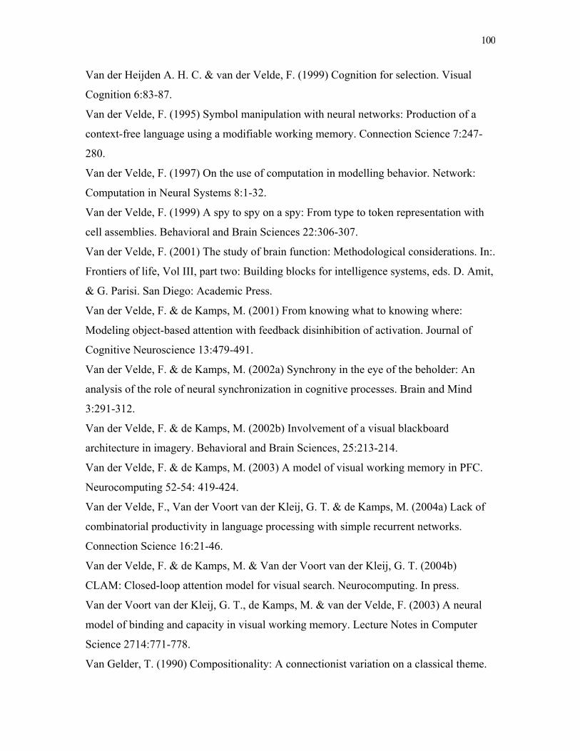
100
Van der Heijden A. H. C. & van der Velde, F. (1999) Cognition for selection. Visual
Cognition 6:83-87.
Van der Velde, F. (1995) Symbol manipulation with neural networks: Production of a
context-free language using a modifiable working memory. Connection Science 7:247-
280.
Van der Velde, F. (1997) On the use of computation in modelling behavior. Network:
Computation in Neural Systems 8:1-32.
Van der Velde, F. (1999) A spy to spy on a spy: From type to token representation with
cell assemblies. Behavioral and Brain Sciences 22:306-307.
Van der Velde, F. (2001) The study of brain function: Methodological considerations. In:.
Frontiers of life, Vol III, part two: Building blocks for intelligence systems, eds. D. Amit,
& G. Parisi. San Diego: Academic Press.
Van der Velde, F. & de Kamps, M. (2001) From knowing what to knowing where:
Modeling object-based attention with feedback disinhibition of activation. Journal of
Cognitive Neuroscience 13:479-491.
Van der Velde, F. & de Kamps, M. (2002a) Synchrony in the eye of the beholder: An
analysis of the role of neural synchronization in cognitive processes. Brain and Mind
3:291-312.
Van der Velde, F. & de Kamps, M. (2002b) Involvement of a visual blackboard
architecture in imagery. Behavioral and Brain Sciences, 25:213-214.
Van der Velde, F. & de Kamps, M. (2003) A model of visual working memory in PFC.
Neurocomputing 52-54: 419-424.
Van der Velde, F., Van der Voort van der Kleij, G. T. & de Kamps, M. (2004a) Lack of
combinatorial productivity in language processing with simple recurrent networks.
Connection Science 16:21-46.
Van der Velde, F. & de Kamps, M. & Van der Voort van der Kleij, G. T. (2004b)
CLAM: Closed-loop attention model for visual search. Neurocomputing. In press.
Van der Voort van der Kleij, G. T., de Kamps, M. & van der Velde, F. (2003) A neural
model of binding and capacity in visual working memory. Lecture Notes in Computer
Science 2714:771-778.
Van Gelder, T. (1990) Compositionality: A connectionist variation on a classical theme.
101
Cognitive Science 14:355-384.
Van Valin, R. D. Jr. (2001) An introduction to syntax. Cambridge: Cambridge University
Press.
Von der Malsburg, C. (1987) Synaptic plasticity as basis of brain organization. In: The
Neural and Molecular Bases of Learning, eds. J. P. Changeux and M. Konishi.
Chichester: John Wiley.
Webelhuth, G. ed. (1995) Government and binding theory and the minimalist program.
Oxford: Blackwell.
Wilson, F.A.W., Ó Scalaidhe, S. P., & Goldman-Rakic, P. S. (1993) Dissociation of
object and spatial processing domains in primate prefrontal cortex. Science 260:1955-
1958.
Wilson, H. R., & Cowan, J. D. (1972) Excitatory an inhibitory interactions in localized
populations of model neurons. Biophysical Journal 12:1-24.
Yakovlev, V. Fusi, S., Berman, E. & Zohary, E. (1998) Inter-trial neuronal activity in
inferior temporal cortex: A putative vehicle to generate long-term associations. Nature
Neuroscience 1:310-317.
Appendix
A1. The architecture for sentence structure
The simulations presented in figure 8 are based on excitatory (E) and inhibitory (I)
neuron populations (e.g., Wilson and Cowan 1972; Gerstner 2000). The activation of
population i is modelled with the population rate Ai, defined as the fraction of neurons
that fire in the time interval [t, t+dt] divided by dt. Ai is given by:
)( jijjii AwFA
dtdA
Σ+−=ατ (1)
τE (α=E) = 10 ms and τI (α=I) = 5 ms are the time constants for the excitatory and
inhibitory populations. The ijw (or ijw → ) are the efficacies from population j onto
population i ( ijw is negative iff j is an inhibitory population). F(x) is given by:
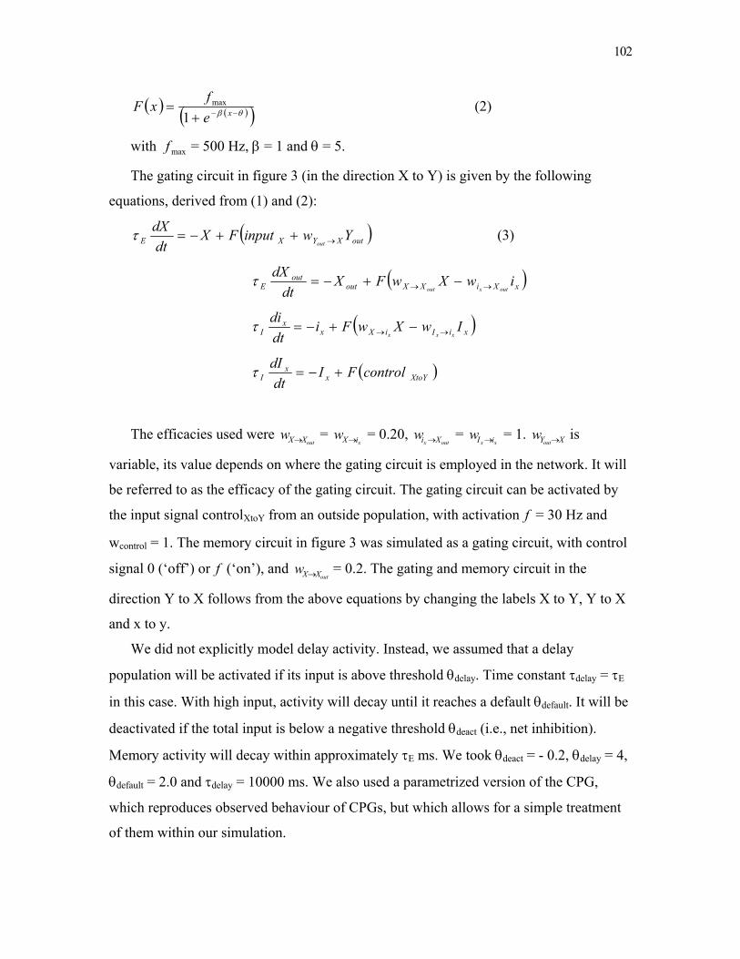
102
( ) ( )( )θβ −−+= xe
fxF1
max (2)
with maxf = 500 Hz, β = 1 and θ = 5.
The gating circuit in figure 3 (in the direction X to Y) is given by the following
equations, derived from (1) and (2):
( )outXYXE YwinputFXdtdX
out →++−=τ (3)
( )xXiXXout
outE iwXwFX
dtdX
outxout →→ −+−=τ
( )xiIiXx
xI IwXwFi
dtdi
xxx →→ −+−=τ
( )XtoYx
xI controlFI
dtdI
+−=τ
The efficacies used were outXXw → =
xiXw → = 0.20, outx Xiw → =
xx iIw → = 1. XYoutw → is
variable, its value depends on where the gating circuit is employed in the network. It will
be referred to as the efficacy of the gating circuit. The gating circuit can be activated by
the input signal controlXtoY from an outside population, with activation f = 30 Hz and
wcontrol = 1. The memory circuit in figure 3 was simulated as a gating circuit, with control
signal 0 (‘off’) or f (‘on’), and outXXw → = 0.2. The gating and memory circuit in the
direction Y to X follows from the above equations by changing the labels X to Y, Y to X
and x to y.
We did not explicitly model delay activity. Instead, we assumed that a delay
population will be activated if its input is above threshold θdelay. Time constant τdelay = τE
in this case. With high input, activity will decay until it reaches a default θdefault. It will be
deactivated if the total input is below a negative threshold θdeact (i.e., net inhibition).
Memory activity will decay within approximately τE ms. We took θdeact = - 0.2, θdelay = 4,
θdefault = 2.0 and τdelay = 10000 ms. We also used a parametrized version of the CPG,
which reproduces observed behaviour of CPGs, but which allows for a simple treatment
of them within our simulation.
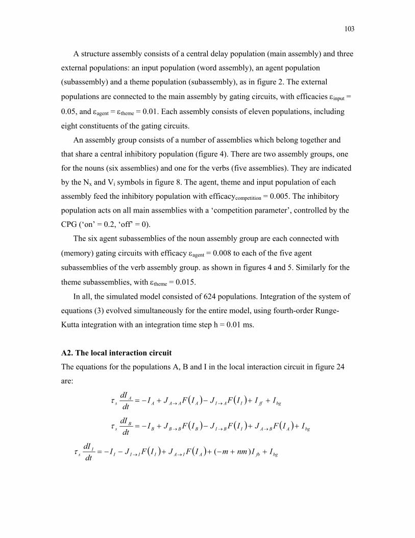
103
A structure assembly consists of a central delay population (main assembly) and three
external populations: an input population (word assembly), an agent population
(subassembly) and a theme population (subassembly), as in figure 2. The external
populations are connected to the main assembly by gating circuits, with efficacies εinput =
0.05, and εagent = εtheme = 0.01. Each assembly consists of eleven populations, including
eight constituents of the gating circuits.
An assembly group consists of a number of assemblies which belong together and
that share a central inhibitory population (figure 4). There are two assembly groups, one
for the nouns (six assemblies) and one for the verbs (five assemblies). They are indicated
by the Nx and Vi symbols in figure 8. The agent, theme and input population of each
assembly feed the inhibitory population with efficacycompetition = 0.005. The inhibitory
population acts on all main assemblies with a ‘competition parameter’, controlled by the
CPG (‘on’ = 0.2, ‘off’ = 0).
The six agent subassemblies of the noun assembly group are each connected with
(memory) gating circuits with efficacy εagent = 0.008 to each of the five agent
subassemblies of the verb assembly group. as shown in figures 4 and 5. Similarly for the
theme subassemblies, with εtheme = 0.015.
In all, the simulated model consisted of 624 populations. Integration of the system of
equations (3) evolved simultaneously for the entire model, using fourth-order Runge-
Kutta integration with an integration time step h = 0.01 ms.
A2. The local interaction circuit
The equations for the populations A, B and I in the local interaction circuit in figure 24
are:
( ) ( ) bgffIAIAAAA
As IIIFJIFJI
dtdI
++−+−= →→τ
( ) ( ) ( ) bgABAIBIBBBB
Bs IIFJIFJIFJI
dtdI
++−+−= →→→τ
( ) ( ) bgfbAIAIIIII
s IInmmIFJIFJIdtdI
++−++−−= →→ )(τ

104
Here, Ix is input current in population x and τs is the synaptic time constant (5ms).
The efficacies Jx are: JA→A = 0.01, JA→B = 0.07, JA→I =0.3, JB→B = 0.01, JI→I = 0.01 and
JI→A = 0.01, JI→B = 0.1. The background activity to all populations is 3,4 Hz (Ibg = 0.01).
The stimulus is given by a feedforward input activity Iff = 25 Hz to population A.
Feedback is given by the cue-related activity Ifb = 25 Hz to population I, divided in the
fractions match n and nonmatch nm (with n + nm = 1) as determined on the basis of
figure 23 (interaction).