neep hvac load shape report final august2
TRANSCRIPT

NEEP i August 2, 2011
C&I Unitary HVAC Load Shape Project
Final Report
August 2, 2011 Version 1.1
Prepared for the Regional Evaluation, Measurement
and Verification Forum a project facilitated by Northeast Energy Efficiency Partnerships (NEEP)
Submitted to NEEP
Northeast Energy Efficiency Partnerships, Inc.
91 Hartwell Avenue
Lexington, MA 02421
Prepared by KEMA
KEMA, Inc.
155 Grand Ave, Suite 500
Oakland, CA 94612
Fax: (510) 891-0440

NEEP ii August 2, 2011
Table of Contents
List of Tables ................................................................................................................... iii
List of Figures ..................................................................................................................iv
0 Executive Summary ................................................................................................. 5
0.1 Methodology and Sample Design ...................................................................... 5
0.2 Data Collection and Unit Analysis ...................................................................... 7
0.3 Load Shape Analysis ......................................................................................... 8
0.4 Results ............................................................................................................... 9
1 Introduction ............................................................................................................ 15
1.1 Project Intent and Goals ................................................................................... 15
1.2 Overall Approach ............................................................................................. 16
2 Methodology .......................................................................................................... 17
2.1 Planning and Sampling .................................................................................... 17
2.1.1 Procurement of Program Administrator and Secondary Data .................... 17 2.1.2 Sample Design .......................................................................................... 19
2.1.2.1 Size Dimensions ................................................................................. 20 2.1.2.2 Regions and Choice of Weather Data ................................................. 20 2.1.2.3 Facility Type Dimension ...................................................................... 31 2.1.2.4 Outside Air Intake Dimension .............................................................. 31 2.1.2.5 Planned Sample Design ...................................................................... 32
2.1.1 Achieved Population and Sample .............................................................. 36 2.2 Data Collection ................................................................................................. 40
2.2.1 Sample Selection and Customer Recruitment ........................................... 40 2.2.2 Site Data Collection ................................................................................... 40 2.2.3 Secondary Data Collection ........................................................................ 45
2.3 Data Analysis ................................................................................................... 47
2.3.1 Quality Control ........................................................................................... 47 2.3.2 Unit Level Regression Modeling Approach ................................................ 48 2.3.1 Definition of Analysis Time Variables ........................................................ 50 2.3.2 Peak Period Definitions ............................................................................. 50 2.3.3 Holidays ..................................................................................................... 53 2.3.4 Extrapolation Out of Sample ...................................................................... 54
3 Results ................................................................................................................... 56
3.1 Normalized Study Results and Basis of Load Shape Tool ............................... 57
3.2 Additional Results ............................................................................................ 63
3.3 Data Summary ................................................................................................. 66

NEEP iii August 2, 2011
4 Description of HVAC Load Shape Tool and Final Data Set ................................... 73
4.1 Overview of HVAC Load Shape Tool ............................................................... 73
4.2 Instructions for obtaining and using HVAC Load Shape Tool .......................... 73
4.3 Step-By-Step Instructions................................................................................. 73
4.4 Overview of Data Set Available to Sponsors .................................................... 74
5 Appendix ................................................................................................................ 75
5.1 C&I Unitary HVAC Data Request Submitted to Forum Members ..................... 75
5.2 Statistical Model References ............................................................................ 77
5.3 Analysis Definitions Supporting Tables ............................................................ 77
5.4 Data Collection Form ....................................................................................... 80
List of Tables Table 0-1: Sample of Units and Connected Load by Region and Size Strata .............................. 7
Table 0-2: Annual Load Factor and EFLH Estimate by Region Totals ....................................... 10
Table 0-3: Load Ratio Estimate by Region Small Units .............................................................. 10
Table 0-4: Load Ratio Estimate by Region Large Units .............................................................. 10
Table 0-5: Coincidence Factor for Peak Demand Definitions by Region Totals ......................... 12
Table 0-6: Coincidence Factor for Peak Demand Definitions by Region Small Units ................. 13
Table 0-7: Coincidence Factor for Peak Demand Definitions by Region Large Units ................. 13
Table 2-1: Summary of Tracking Data Provided by Sponsors .................................................... 18
Table 2-2: CDD and THIDD Data by City and Zone ................................................................... 22
Table 2-3: Weather Region Categorizations ............................................................................... 23
Table 2-4: Required Sample Sizes for Considered Error Ratios and Precisions ........................ 33
Table 2-5: Planned Sample Sizes and Precisions at the 90% Confidence Interval for Primary Data Collection ............................................................................................................................ 34
Table 2-6: Planned Sample Sizes for Primary Data Collection ................................................... 35
Table 2-7: Population of Units and Connected Load by Region and Size Strata ....................... 36
Table 2-8: Sample of Units and Connected Load by Region and Size Strata ............................ 37
Table 2-9: Sample of Units and Connected Load Included in Analysis ...................................... 38
Table 2-10: Metered Sample of Units and Connected Load By Sponsor ................................... 39
Table 2-11: Metering Equipment Suite for one AC Unit .............................................................. 41
Table 2-12: Distribution of Leveraged Data ................................................................................ 46
Table 2-13: ISO-NE System Peak to Weather Regression Results............................................ 52
Table 2-14: Number of TMY3 Hours with Load Greater than 90% of Long term Average and Comparison to Number of FCM Seasonal Peak Hours (2008-10) .............................................. 52
Table 2-15: Final Set of FCM Season Peak Hours ..................................................................... 53
Table 3-1: Annual Load Factor and EFLH Estimate by Region Totals ....................................... 57
Table 3-2: Coincidence Factor for Peak Demand Definitions by Region Totals ......................... 58

NEEP iv August 2, 2011
Table 3-3: Load Ratio Estimate by Region Small Units .............................................................. 59
Table 3-4: Coincidence Factor for Peak Demand Definitions by Region Small Units ................. 60
Table 3-5: Load Ratio Estimate by Region Large Units .............................................................. 61
Table 3-6: Coincidence Factor for Peak Demand Definitions by Region Large Units ................. 62
Table 3-7: Sample of Units and Metered Connected Load by Building Type and Size .............. 66
Table 3-8: Annual Energy Estimate by Building Type ................................................................. 67
Table 3-9: Coincidence Factor Estimate by Building Type ......................................................... 68
Table 3-10: Sample of Units and Connected Load by Economizer Type and Size .................... 71
Table 3-11: Annual Energy Estimate by Economizer Type with Standard Error......................... 71
Table 3-12: Coincidence Factor Estimate by Economizer Type with Standard Error ................. 72
Table 5-1: Mean /Standard Deviation of ISO-NE Actual Peak and 50/50 Forecast .................... 77
Table 5-2: ISO-NE FCM Seasonal Peak Data and Analysis Summary ...................................... 79
List of Figures Figure 2-1: Northern New England (NE-North) Sites and Assigned Weather Stations ............... 24
Figure 2-2: Southern New England (NE-South) Sites and Assigned Weather Stations ............. 25
Figure 2-3: New England – Eastern Massachusetts (NE-East Mass) Sites and Assigned Weather Stations ........................................................................................................................ 26
Figure 2-4: Mid-Atlantic Sites and Assigned Weather Stations .................................................. 27
Figure 2-5: New York Urban Coastal (NY-Urban/Coastal) Sites and ......................................... 28
Figure 2-6: New York Inland (NY-Inland) Sites and Assigned Weather Stations ........................ 29
Figure 2-7: TMY3 Weather Stations Assigned to Sites ............................................................... 29
Figure 2-8: Metering Equipment Picture ..................................................................................... 43
Figure 2-9: Wattnode Status Indicator Lights .............................................................................. 44
Figure 3-1: Annual Small Unit Load Shapes Shown as Energy Prints ....................................... 64
Figure 3-2: Annual Large Unit Load Shapes Shown as Energy Prints ....................................... 65
Figure 5-1: Historical FCM Peak Data and Forecast .................................................................. 78

NEEP 5 August 2, 2011
0 Executive Summary This C&I Unitary HVAC Load Shape Project developed weather normalized 8,760 (representing
every hour of the year) cooling end-use load shapes representative of hourly savings for the
target population of efficient unitary HVAC equipment promoted by efficiency programs in the
New England, New York and mid-Atlantic regions. Given the trade-offs between up-front capital
costs and continuing operating costs, unitary HVAC is generally chosen for situations with
minimal internal cooling loads, and where operating hours are not large and are concentrated in
the summer. Unitary HVAC is one type of cooling equipment, with relatively low capital costs
but high operating costs. Where cooling loads are more evenly distributed throughout the year
and cover substantial internal heat gains, other types of cooling equipment - with higher capital
costs, but lower operating costs, are typically chosen. These other types include (by ascending
efficiency) air-to-air air conditioners and heat pumps, water-to-air heat pumps, and chillers.
The unitary HVAC load shapes developed in this project further support program administrator
calculations of savings in the forward capacity markets. These load shapes were based on
results of primary data collection, including metering, completed as part of this study, as well as
data available from existing sources. Not all Forum sponsors were able to provide sites for
metering. However, by design and intent, the study goal was to serve all Forum members with
results that are transferable within the Forum overall including those not able to provide sites for
metering.
0.1 Methodology and Sample Design The sampling and analysis results were developed relative to the key dimensions of unit size
and unit location. The sampling framework was devised to meet the needs of sponsors and
allow for determination of average coincident peak demand impacts according to independent
system operator definitions and confidence/precision criteria. Data to establish the sample
frame was received from 13 sponsors and 11 of those sponsors had data meeting the minimum
study requirements. HVAC metered data was available from three sponsors, but only the BG&E
Commercial AC Profiler project had data for units meeting the study criteria. All other C&I
HVAC data identified in the NEEP Phase I Load Shape Project1 was identified as representing
larger or custom systems not characterized as “Unitary C&I HVAC from 1 to 100 ton”. The
study population excluded units with rebated economizers, devices which optimize the amount 1 The End Use Load Data Update Project – Final Report Phase 1, 2009, by KEMA for NEEP and
Regional EM&V Forum sponsors, is available at www.neep.org/emv-forum/forum-products-and-
guidelines.

NEEP 6 August 2, 2011
of fresh outside air drawn into cooled spaces. For multiple sponsors this only included dual-
enthalpy economizers which have temperature and humidity sensors both outdoors at the unit
and indoors in the cooled space. For a few sponsors this included rebated economizers of
unknown type. The economizers were excluded because the savings claim for those measures
are based on reducing the normal operating hours of the high efficiency equipment and
inclusion required oversampling that was outside the scope of the study.
The unit installed cooling capacity, its “size”, was used to develop a small and large sampling
dimension based on prior studies and experience that larger units have different annual full load
hours and peak coincidence timing. The units also are bi-furcated into small and large based on
the fact that large units (between 11.5 and 100 nominal tons cooling) have multiple compressors
and fans that operate in stages while a majority of small units (between 1 and 11.25 tons) are
single stage units. The size cut point conforms to the ASHRAE 90.1 (2007) size class
designations which set the minimum efficiency for new equipment based on nominal installed
capacity range.
A set of six weather region categories met the need to minimize the number of weather regions
while maintaining meaningful weather categorizations and staying within the task budget. A
representative city with typical meteorological year (TMY3) weather data available would then
be chosen for each weather region to provide normalized weather. The unit level regression
models used the TMY3 weather data as inputs to weather normalize predicted loads which were
based on actual metered year weather and also extrapolate data outside the metering period.
The TMY3 weather files are developed to represent typical hourly conditions based on 15 years
of data for a particular station. They represent conditions for annual energy computer
simulations and do not represent extreme design conditions nor are they simply the average
with no extreme hours or days.
The sample was designed to achieve minimum peak demand estimate precisions of 10% at the
90% confidence interval for the aggregate Loadshape which would require 133 to 530 sampled
units depending on error ratio. An error ratio of 1.0 was chosen for small units and 0.6 for large
units to achieve the desired precisions for peak demand estimates as well as annual load
shapes based on review of all the available information from past studies. The error ratio
measures the population variability of unit level demand relative to the connected load of the
HVAC unit. The connected load is defined as the unit’s rated load used in the calculation of
energy efficiency rating (EER) defined by American Heating and Refrigeration Institute (AHRI)
standards 210/240. The connected load of the HVAC unit was obtained from tracking data
directly or accurately through unit make and model number for the majority of A/C units in the

NEEP 7 August 2, 2011
study population. All connected loads in the analysis were estimated based on tonnage and unit
EER.
The unit-level sample was designed such that total sample would be evenly allocated by
weather region and within regions proportional to the population count for allocation by size for
small and large units. This design was chosen given the limitation of having incomplete data on
existing stratum-specific estimates of error ratios that could inform this study’s design. Through
multiple meetings the Forum came to agreement on a sample design of 45 small units and 30
large units for each of 6 weather regions for a total sample size of 450 units which would be
supplemented by some available data for small units from the BG&E AC Profiler study. The
following table describes the total achieved sample including the data leveraged from previous
studies. As previously mentioned, only data from the BG&E Commercial AC Profiler study was
applicable and most of the data fell under the small unit category. This study actually metered
22 units in the Mid-Atlantic small-stratum and leveraged existing metering data on 101 units
from BG&E as shown in the table.
Table 0-1: Sample of Units and Connected Load by Region and Size Strata
Includes Leveraged Data
0.2 Data Collection and Unit Analysis Following sample design, primary and backup samples were chosen for the purpose of
scheduling metering installation and data collection site visits. The installation of meters began
in May and ended in early June. All meters were removed in October. Data was collected for all
HVAC units specified in the final sample design and selection in adherence to the on-site
Region Small Large Total Small Large Total
Mid-Atlantic - BGE 95 6 101 516.4 91.8 608.3
Mid-Atlantic - Metered 22 15 37 257.2 361.5 165.3
Region Small Large Total Small Large Total
Mid-Atlantic 117 21 138 773.6 453.3 1,226.9
NE-East Mass 45 30 75 260.1 567.1 827.2
NE-North 45 30 75 251.8 664.2 916.0
NE-South Coastal 47 31 78 291.3 739.2 1,030.6
NY- Inland 44 33 77 252.7 438.3 691.0
NY- Urban/Coastal 44 24 68 383.1 383.8 766.9
Total 348 163 511 2,212.7 3,245.8 5,458.5
Metered Connected Load (kW)Metered Sample Size "n" (Count)
Metered Sample Size "n" (Count) Metered Connected Load (kW)

NEEP 8 August 2, 2011
measurement protocols. The project recognized the critical importance of full compliance with
all state and regional measurement requirements. The power measurement equipment
complied with ISO New England and PJM Interconnection M&V protocols2. The data collection
also included unit nameplate information, outside air control type, control settings, site building
type, and data logger configuration.
Beginning with the removal of the first meters in October, regression modeling began. Each unit
was modeled individually, taking into account factors such as day type, sequential hot days, and
unique temperatures and humidity. All system fan usage during compressor and condenser
“cooling” operation was included in the analysis. Peak coincidence factors and annual full load
hours were defined to only include the cooling operation of unitary HVAC equipment and thus
fan-only usage of systems was excluded from analyses.
The regression models were then used with a TMY3 full year normal weather series to generate
normalized 8,760 hourly results. The load predicted by the model was set to zero if the THI was
less than 50°F. This decision was made based on review of the BGE AC profiler data which
included year round data collection for multiple years and usage during off-peak metered
periods. This restriction had no effect on summer peaks, only on off-peak and annual usage.
Any information collected about when the units are activated or shut down for winter was
applied when extrapolating the results. If a unit was designated as being turned on in March
and off in December then no modeled usage was calculated for January and February. At this
stage there is a unit level 8760 weather-normalized profile for each sample point.
0.3 Load Shape Analysis After all the unit level modeling was done and regional weather normalization completed, each
load shape profile was pooled into 12 strata determined by 6 regions and 2 unit sizes (small
<11.25 tons or large ≥11.25 tons). For each hour, the load for each stratum was calculated as
the sum of the sample loads multiplied by their case weights. For each stratum, the case-
weighted sample connected load was also calculated. The ratio of the total hourly load to the
total connected load derived from the sample data in each stratum was multiplied by the total
population connected load to estimate the total stratum hourly load. By performing this
calculation for every hour, an annual load profile was estimated. The variation in the sample
customer ratios in each hour, as well as the sample size was used to calculate the relative
2 New England Independent System Operator (ISO-NE) M&V Manual for Wholesale Forward Capcity
Market (FCM). www.iso-ne.com/rules_proced/isone_mnls/index.html
PJM Manual 18B:Energy Efficiency Measurement & Verification, Revision: 01
Effective Date: March 1, 2010 http://pjm.com/~/media/documents/manuals/m18b.ashx

NEEP 9 August 2, 2011
precision at the 90% confidence interval of each hourly estimate. The analysis results were
used to develop a savings workbook (the Loadshape Tool), which will allow sponsors to
generate demand and energy savings over desired time intervals based on a connected load
reduction input.
0.4 Results The following tables present the annual usage and coincident peak estimates and relative
precisions based on the developed load shapes. The data are normalized by connected load
(based on EER and tonnage rating) such that the results are unit-less, coincidence and annual
load factors, except for effective full load cooling hours. All tables include estimated factors or
full load hours. Each estimated factor is presented with the relative precision of each estimate at
the 80% and 90% two-tail confidence intervals, abbreviated respectively as “RP @ 80%CI” and
“RP @ 90%CI. As a reminder, relative precision at the 80% two-tail interval is equivalent to that
of the 90% one-tail.
The following table presents the annual load factor and effective full load hours for the regional
totals and the relative precisions of the estimates. The annual load factor represents the
fraction of hourly regional loadshape divided by connected load for all 8,760 hours or more
simply, the fraction of effective full load cooling hours3 (EFLH) over 8,760.
760,8
)(
)(8760
1
EFLHFactorAnnualLoad
kWLoadConnected
kWLoadHourlyEstimatedEFLH
h
The relative precisions of the two estimates are identical given there is only division by a
constant. The precisions were much lower than the planned precisions from the sample design
for peak demand factors. As shown below, precisions for all of the load-weighted regional totals
are less than 18%. The precision calculations are based on aggregation of the hourly estimates
and hourly error terms and can be replicated in detail in the Load Shape Tool.
3 Effective full load cooling hours (EFLH) represents the annual number of hours (8,760 hours = 1 year)
that a cooling system would operate for, at full load. It can be used to estimate annual energy
consumption of a system when the capacity and efficiency are known.

NEEP 10 August 2, 2011
Table 0-2: Annual Load Factor and EFLH Estimate by Region Totals4
Table 0-3: Load Ratio Estimate by Region Small Units4
Table 0-4: Load Ratio Estimate by Region Large Units4
4 Note that relative precision (RP) at the 80% two-tail interval is equivalent to that of the RP 90% one-tail.
Total
RegionEstimated
RatioRP @ 80%CI
RP @ 90%CI
Annual Estimate
RP @ 80%CI
RP @ 90%CI
Mid-Atlantic 0.1707 ±9.78% ±12.55% 1,495 ±9.78% ±12.55%
NE-East Mass 0.1339 ±10.12% ±12.99% 1,173 ±10.12% ±12.99%
NE-North 0.0862 ±13.14% ±16.87% 755 ±13.14% ±16.87%
NE-South Coastal 0.0976 ±11.44% ±14.69% 855 ±11.44% ±14.69%
NY- Inland 0.1087 ±13.58% ±17.43% 952 ±13.58% ±17.43%
NY- Urban/Coastal 0.1704 ±10.69% ±13.72% 1,492 ±10.69% ±13.72%
Annual Load Factor (EFLH/8760)
EFLH = Effective Full Load Cooling Hours
SMALL units (<11.25 TONS)
Small Units
RegionEstimated
RatioRP @ 80%CI
RP @ 90%CI
Annual Estimate
RP @ 80%CI
RP @ 90%CI
Mid-Atlantic 0.1157 ±6.79% ±8.72% 1,014 ±6.79% ±8.72%
NE-East Mass 0.1261 ±14.78% ±18.97% 1,104 ±14.78% ±18.97%
NE-North 0.0946 ±19.18% ±24.62% 829 ±19.18% ±24.62%
NE-South Coastal 0.1064 ±14.98% ±19.22% 932 ±14.98% ±19.22%
NY- Inland 0.0752 ±25.39% ±32.59% 659 ±25.39% ±32.59%
NY- Urban/Coastal 0.1375 ±8.27% ±10.62% 1,204 ±8.27% ±10.62%
Annual Load Factor (EFLH/8760) EFLH
LARGE units (≥ 11.25 TONS)
Large Units
RegionEstimated
RatioRP @ 80%CI
RP @ 90%CI
Annual Estimate
RP @ 80%CI
RP @ 90%CI
Mid-Atlantic 0.2081 ±13.24% ±16.99% 1,823 ±13.24% ±16.99%
NE-East Mass 0.1396 ±13.67% ±17.54% 1,223 ±13.67% ±17.54%
NE-North 0.0775 ±17.26% ±22.15% 679 ±17.26% ±22.15%
NE-South Coastal 0.0905 ±17.21% ±22.09% 793 ±17.21% ±22.09%
NY- Inland 0.1215 ±15.69% ±20.13% 1,065 ±15.69% ±20.13%
NY- Urban/Coastal 0.1894 ±14.78% ±18.97% 1,659 ±14.78% ±18.97%
EFLHAnnual Load Factor
(EFLH/8760)

NEEP 11 August 2, 2011
The definition of the ISO-NE On-Peak, PJM On-Peak, and ISO-NE FCM seasonal coincident
peak factor are described below:
ISO-NE On-Peak Period: The ISO-NE summer “Demand Resource On-Peak Hours,” are defined as 1 PM to 5 PM on weekday non-holidays during June, July, and August.
PJM On-Peak Period: The PJM On-Peak Period is structurally identical to the first,
except that it will encompass the hours from 2 PM to 6 PM instead of 1 PM to 5 PM.
ISO-NE FCM Seasonal Peak: The FCM Summer Seasonal Peak includes all non-
holiday weekday hours in June, July and August during which the ISO New England
Real-Time System Hourly Load is greater than 90% of the most recent “50/50” System
Peak Load Forecast for the summer season.
A coincident peak factor of one would indicate all units ran at full load for the entire hour for all
hours included in the peak definitions. The following table presents coincident factor estimates
and precisions and the maximum hourly coincident load ratio and relative precisions for those
hours. The precisions at the 90% confidence interval of the coincident peak estimates range
roughly from 9% to 16%. They are low relative to the planned precisions across all peak
definitions and regions. The precision of the maximum load ratio is for an individual hour by
region and shows the greater variability at the hourly level with precisions from 6% to 17%. The
coincidence factor estimates include the effects of oversizing and some peak defined hours
where units operate at part loads. The results reflect diversity of usage within and between
hours in the population.

NEEP 12 August 2, 2011
Table 0-5: Coincidence Factor for Peak Demand Definitions by Region Totals4
Total
RegionHourly
AverageRP @ 80%CI
RP @ 90%CI
Hourly Maximum
RP @ 80%CI
RP @ 90%CI
Mid-Atlantic 0.4892 ±7.09% ±9.10% 0.718 ±7.83% ±10.05%
NE-East Mass 0.4488 ±8.40% ±10.78% 0.699 ±8.43% ±10.82%
NE-North 0.3421 ±11.98% ±15.38% 0.469 ±12.23% ±15.69%
NE-South Coastal 0.3397 ±10.39% ±13.33% 0.526 ±9.59% ±12.30%
NY- Inland 0.3815 ±12.59% ±16.15% 0.477 ±13.01% ±16.69%
NY- Urban/Coastal 0.5529 ±8.24% ±10.58% 0.822 ±5.80% ±7.44%
Mid-Atlantic 0.4833 ±7.32% ±9.40% 0.718 ±7.83% ±10.05%
NE-East Mass 0.4443 ±8.56% ±10.99% 0.699 ±8.43% ±10.82%
NE-North 0.3343 ±12.16% ±15.61% 0.469 ±12.23% ±15.69%
NE-South Coastal 0.3341 ±10.49% ±13.46% 0.526 ±9.59% ±12.30%
NY- Inland 0.3836 ±12.62% ±16.20% 0.477 ±13.01% ±16.69%
NY- Urban/Coastal 0.5665 ±7.83% ±10.05% 0.822 ±5.80% ±7.44%
Mid-Atlantic
NE-East Mass 0.4863 ±8.39% ±10.77% 0.699 ±8.43% ±10.82%
NE-North 0.4241 ±12.23% ±15.70% 0.469 ±12.23% ±15.69%
NE-South Coastal 0.4369 ±9.54% ±12.24% 0.526 ±9.59% ±12.30%
NY- Inland
NY- Urban/Coastal
ISO-NE FCM
Seasonal Peak
ISO-NEOn-Peak (1-5PM, WDNH, Jun-Aug)
Maximum Load Ratio
PJMOn-Peak (2-6PM, WDNH, Jun-Aug)
Coincidence Factor

NEEP 13 August 2, 2011
Table 0-6: Coincidence Factor for Peak Demand Definitions by Region Small Units4
Table 0-7: Coincidence Factor for Peak Demand Definitions by Region Large Units4
Small Units
RegionHourly
AverageRP @ 80%CI
RP @ 90%CI
Hourly Maximu
mRP @ 80%CI
RP @ 90%CI
Mid-Atlantic 0.3578 ±5.54% ±7.11% 0.588 ±5.70% ±7.32%
NE-East Mass 0.4345 ±12.38% ±15.89% 0.722 ±10.40% ±13.35%
NE-North 0.3720 ±16.23% ±20.84% 0.501 ±15.91% ±20.42%
NE-South Coastal 0.3498 ±13.09% ±16.80% 0.536 ±12.38% ±15.89%
NY- Inland 0.2426 ±22.73% ±29.18% 0.305 ±22.31% ±28.63%
NY- Urban/Coastal 0.4435 ±7.50% ±9.63% 0.703 ±7.69% ±9.87%
Mid-Atlantic 0.3596 ±5.57% ±7.16% 0.588 ±5.70% ±7.32%
NE-East Mass 0.4305 ±12.54% ±16.09% 0.722 ±10.40% ±13.35%
NE-North 0.3623 ±16.24% ±20.85% 0.501 ±15.91% ±20.42%
NE-South Coastal 0.3357 ±13.62% ±17.49% 0.536 ±12.38% ±15.89%
NY- Inland 0.2433 ±22.70% ±29.14% 0.305 ±22.31% ±28.63%
NY- Urban/Coastal 0.4507 ±7.38% ±9.47% 0.703 ±7.69% ±9.87%
Mid-Atlantic
NE-East Mass 0.4758 ±12.31% ±15.80% 0.722 ±10.40% ±13.35%
NE-North 0.4519 ±16.20% ±20.79% 0.501 ±15.91% ±20.42%
NE-South Coastal 0.4311 ±13.62% ±17.48% 0.536 ±12.38% ±15.89%
NY- Inland
NY- Urban/Coastal
ISO-NE FCM
Seasonal Peak
PJMOn-Peak (2-6PM, WDNH, Jun-Aug)
ISO-NEOn-Peak (1-5PM, WDNH, Jun-Aug)
Maximum Load RatioCoincidence Factor
Large Units
RegionHourly
AverageRP @ 80%CI
RP @ 90%CI
Hourly Maximum
RP @ 80%CI
RP @ 90%CI
Mid-Atlantic 0.5787 ±9.80% ±12.58% 0.874 ±10.17% ±13.05%
NE-East Mass 0.4591 ±11.33% ±14.55% 0.683 ±12.56% ±16.12%
NE-North 0.3113 ±17.75% ±22.78% 0.438 ±18.65% ±23.93%
NE-South Coastal 0.3314 ±15.70% ±20.16% 0.543 ±14.43% ±18.51%
NY- Inland 0.4348 ±14.49% ±18.59% 0.545 ±15.04% ±19.30%
NY- Urban/Coastal 0.6162 ±11.25% ±14.44% 0.893 ±8.58% ±11.01%
Mid-Atlantic 0.5674 ±10.20% ±13.10% 0.874 ±10.17% ±13.05%
NE-East Mass 0.4543 ±11.58% ±14.87% 0.683 ±12.56% ±16.12%
NE-North 0.3054 ±18.35% ±23.55% 0.438 ±18.65% ±23.93%
NE-South Coastal 0.3328 ±15.48% ±19.87% 0.543 ±14.43% ±18.51%
NY- Inland 0.4375 ±14.53% ±18.64% 0.545 ±15.04% ±19.30%
NY- Urban/Coastal 0.6335 ±10.62% ±13.64% 0.893 ±8.58% ±11.01%
Mid-Atlantic
NE-East Mass 0.4940 ±11.36% ±14.58% 0.683 ±12.56% ±16.12%
NE-North 0.3953 ±18.60% ±23.87% 0.438 ±18.65% ±23.93%
NE-South Coastal 0.4416 ±13.27% ±17.03% 0.543 ±14.43% ±18.51%
NY- Inland
NY- Urban/Coastal
ISO-NE FCM
Seasonal Peak
Coincidence Factor Maximum Load Ratio
ISO-NEOn-Peak (1-5PM, WDNH, Jun-Aug)
PJMOn-Peak (2-6PM, WDNH, Jun-Aug)

NEEP 14 August 2, 2011
Preface The Regional EM&V Forum
The Regional EM&V Forum (Forum) is a project managed and facilitated by Northeast Energy
Efficiency Partnerships, Inc. The Forum’s purpose is to provide a framework for the
development and use of common and/or consistent protocols to measure, verify, track and
report energy efficiency and other demand resource savings, costs and emission impacts to
support the role and credibility of these resources in current and emerging energy and
environmental policies and markets in the Northeast, New York, and Mid-Atlantic region. Jointly
sponsored research is conducted as part of this effort. For more information, see http:
www.neep.org/emv-forum.
Acknowledgments
Jarred Metoyer from KEMA managed the project, assisted by many colleagues. Stephen Waite
served as technical advisor to NEEP throughout this project.
Subcommittee for the Unitary HVAC Loadshape Project
A special thanks and acknowledgment from Elizabeth Titus on behalf of EM&V Forum staff and
contractors is extended to this project’s subcommittee members and beta testers, many of
whom provided input during the development of this project: Iqbal Al-Azad and Jim Cunningham
(New Hampshire Public Utility Commission), Dave Bebrin, Tom Belair, and Gene Fry (Northeast
Utilities), Judeen Byrne, Victoria Engel-Fowles and Helen Kim (NYSERDA), Mary Cahill (New
York Power Authority), Elizabeth Crabtree (Efficiency Maine), Niko Dietsch (US EPA), Kristy
Fleischmann, Mary Straub and Sheldon Switzer (Baltimore Gas and Electric), Ethan Goldman
and Nikola Janjic (VEIC - Efficiency Vermont), Kristin Graves (Consolidated Edison), Paul Gray
(United Illuminating), Colin High (Metro Washington Council of Governments), Doug Hurley
(consultant to Cape Light Compact), Dave Jacobson and Andrew Wood (National Grid), Debbie
Kanner, Teri Lutz and Gary Musgrave (Allegheny Power), Taresa Lawrence (District of
Columbia Department of Energy), Laura Magee (PepCo Holding Company), Arthur Maniaci
(New York ISO), Kim Oswald (consultant to CT Energy Efficiency Board), Ralph Prahl
(consultant to MA Energy Efficiency Advisory Council), Allison Reilly (NESCAUM), Marilyn Ross
(Massachusetts Public Service Commission), Earle Taylor (consultant to Northeast Utilities),
and Dave Weber (NSTAR).

NEEP 15 August 2, 2011
1 Introduction This report serves the following functions:
Document the intent and goals of this Unitary HVAC Load Shape Project
Provide an overview of project activities and analysis methods
Present selected results from the load shape analysis tool
Present additional results based on analysis of the data set.
1.1 Project Intent and Goals The primary goal of this project was to develop weather normalized 8,760 (representing every
hour of the year) cooling end-use load shapes representative of hourly savings for the target
population of efficient unitary HVAC equipment promoted by efficiency programs in the New
England, New York and mid-Atlantic regions. Given the trade-offs between up-front capital
costs and continuing operating costs, unitary HVAC is generally chosen for situations with
minimal internal cooling loads, and where operating hours are not large and are concentrated in
the summer. Unitary HVAC is one type of cooling equipment, with relatively low capital costs
but high operating costs. Where cooling loads are more evenly distributed throughout the year
and cover substantial internal heat gains, other types of cooling equipment - with higher capital
costs, but lower operating costs, are typically chosen. These other types include (by ascending
efficiency) air-to-air air conditioners and heat pumps, water-to-air heat pumps, and chillers.
The unitary HVAC load shapes developed in this project further support program administrator
calculations of savings in the forward capacity markets. These load shapes were based on
results of primary data collection, including metering, completed as part of this study, as well as
data available from existing sources.
The sampling and analysis results were developed relative to the key dimensions of unit size
and unit location. The results of this project are delivered in multiple formats: this report, a
savings workbook called the Loadshape Tool, and a data set of complete analysis results and
collected data. This report contains a comprehensive description of the data collection process
and the analytical methods used to develop the results. The savings Loadshape Tool provides
savings load shapes across all key dimensions identified during project sampling. The
Loadshape Tool outputs energy and demand savings estimates over any specified time frame
based on the connected load reduction value entered into the Loadshape Tool. The data set

NEEP 16 August 2, 2011
includes 8760 analysis results for all units in the sample and other data collected for the
metered units.
1.2 Overall Approach This section provides a high level overview of the approach taken to complete this project.
To begin developing a sample frame for the project, a detailed data request was submitted to all
sponsors. This data request asked for tracking information and secondary source data from any
potentially relevant program or research efforts undertaken by sponsors. Using the data
received from this request, a sampling framework was devised to meet the needs of sponsors
and allow for determination of average coincident peak demand impacts according to ISO/PJM
definitions and confidence/precision criteria.
Following sample design, primary and backup samples were chosen for the purpose of
scheduling metering installation and data collection site visits. Scheduling was completed
rapidly in order to capture as much of the cooling season as possible while still maintaining the
integrity of the project sampling requirements. The installation of meters began in May and
ended in early June. All meters were removed in October. Secondary facility data was collected
concurrent with the May meter installations to inform the subsequent HVAC unit regression
modeling.
Beginning with the removal of the first meters in October, regression modeling began. Each unit
was modeled individually, taking into account factors such as day type, sequential hot days, and
unique temperatures and humidity. The regression models were then used with a full year
normal weather series to generate normalized 8,760 results. Unit level normalized results were
aggregated based on the case weights determined during the sampling process. The analysis
results were used to develop a savings workbook (the Loadshape Tool), which will allow
sponsors to generate demand and energy savings over desired time intervals based on a
connected load reduction input.
NEEP 17 August 2, 2011
2 Methodology
2.1 Planning and Sampling
2.1.1 Procurement of Program Administrator and Secondary Data Within one week of the kick off meeting, KEMA prepared and submitted a blanket data request
to the Project Coordinator. This data request specified the required information to characterize
C&I Unitary HVAC programs. The purpose of this data request was to obtain all available
tracking data from unitary HVAC programs undertaken by Forum members within the past three
years. The dimensionality of the sampling frame was dictated by the availability of common
tracking variables across Forum member programs. The study’s focus was on direct refrigerant
expansion (DX) packaged unitary HVAC units installed at non-residential (C&I) facilities.
Several types of efficiency programs were excluded from this data request, in particular:
Custom programs that do not have parsed-out HVAC savings (whole building new
construction programs, for instance).
Programs with HVAC measures that make up less than 5% of a given sponsor’s total
number of unitary HVAC measures.
Programs that include unitary HVAC equipment in excess of 100 tons are only required
to provide savings data for equipment less than or equal to 100 tons. A cap of 100 tons
has been designated for this project because differentiating between unitary and
customized systems greater than 100 tons becomes an issue.
The following information was requested for each applicable Forum member program with
additional details provided in the Appendix Section 5.1:
Tracking savings estimates on a per unit/site basis
Detailed equipment characteristics for each HVAC unit in the population
Site Characteristics
Load Zone / Climate
Program Participant Contact Information
Dated Records
The data were combined into common fields for development of the target population. Units
were required to include installed capacity in tons (size) and efficiency for the purpose of
estimating connected load where the connected load was not explicitly included. The target
population included air-source split systems and packaged rooftop systems. Packaged terminal
air conditioners (PTACS) were excluded along with all water-source and ground-source

NEEP 18 August 2, 2011
equipment. All equipment had to be installed between January 2007 and May 2010 so the
population excluded older units or units not installed in time for metering in summer 2010.
In addition to tracking data, KEMA also requested that load data from recently completed
applicable studies be provided. Due to the diverse nature of the load metering data and results
generated through various programs, KEMA anticipated significant variability in the formatting
and content of the provided metering data, results and documentation. Unit or site level
documentation was to include equipment characteristics, site characteristics, and climate data
according to the same guidelines provided for the tracking data request.
Data to establish the sample frame was received from 13 sponsors and 11 of those sponsors
had data meeting the minimum study requirements. HVAC metered data was available from
three sponsors, but only the BG&E Commercial AC Profiler project had data for units meeting
the study criteria. All other C&I HVAC data identified in the NEEP Phase I Load Shape Project5
was identified as representing larger or custom systems not characterized as “Unitary C&I
HVAC from 1 to 100 ton”. Details of how the sample broke down by sponsor and the amount of
leveraged data is included in the following section. Table 2-1 below details the sponsors who
provided data, those with data qualified as meeting the unitary HVAC definition, and those with
units which were excluded because they also included a rebated economizer. For multiple
sponsors this only included dual-enthalpy economizers which have temperature and humidity
sensors both outdoor at the unit and indoor in the cooled space. For a few sponsors this
included rebated economizers of unknown type. The economizers were excluded because the
savings claim for those measures are based on reducing the normal operating hours of the high
efficiency equipment and inclusion required oversampling that was outside the scope of the
study.
Table 2-1: Summary of Tracking Data Provided by Sponsors
Sponsor Provided
Data Qualifying
Data Economizer Rebate
Units Excluded
Baltimore Gas & Electric (BGE) X X
Cape Light Compact (CLC) X X X
Efficiency Maine (MAINE) X
National Grid (NGRID) X X X
NSTAR X X X
5 The End Use Load Data Update Project – Final Report Phase 1, 2009, by KEMA for NEEP and
Regional EM&V Forum sponsors, is available at www.neep.org/emv-forum/forum-products-and-
guidelines.

NEEP 19 August 2, 2011
Sponsor Provided
DataQualifying
DataEconomizer Rebate
Units Excluded
Northeast Utilities (NU) X X X
New York Power Authority (NYPA) X
NYSERDA X X X
PEPCO X X
Public Service New Hampshire (PSNH) X X X
United Illuminating (UILL) X X
Unitil X X
Efficiency Vermont (VEIC) X X
2.1.2 Sample Design There were a number of dimensions under consideration as the sample design was developed
through the kick off meeting discussions and additional meetings with the Forum. These
dimensions include:
Sampling unit: project, facility, or A/C unit;
Climate: as per temperature data or weather region;
Unit size: tracking savings, connected kW, or tonnage;
Facility or business type;
Unit outside air intake type: Economizers (dual or single enthalpy), fixed, or none
Independent system operator (ISO) Load zone (ISO-NE, NY ISO, and PJM);
Geography: State or Sponsor service territory;
Covering even several of these dimensions created some formidable challenges to the project.
As an example, if we elected to design for four (4) weather/load zones, six (6) facility types, and
stratify by three (3) size (e.g. savings) tiers, we end up with seventy-two (72) domains to cover
with the available sample. KEMA had to work closely with the sponsors to prioritize these
potential stratification dimensions and formulate an appropriately representative sample design
that was affordable within the project budget. The final sample design was reviewed and
approved by consensus from the project subcommittee.
Stratification was ultimately dictated by two factors: (1) the availability of common tracking
variables across sponsor programs from which to devise the sample frame, and (2) the relative
importance of the various possible sample dimensions to the sponsors.

NEEP 20 August 2, 2011
We envisioned a multi-dimensional sample design using some of the dimensions discussed
above. The challenge was to attain adequate coverage of all of the “important” characteristics
(i.e. region, unit size, building type, etc.) that can be isolated for the population of program
participants. This required consistency across the data elements secured for each of the
sponsors.
After discussion with the project subcommittee, designing the samples and selecting the
participants based on overall targets across all of the sponsors’ service territories and ISO load
zones was chosen as the sample design strategy. The following section discusses each of the
key parameters used and considered in the study.
2.1.2.1 Size Dimensions Typically, these types of studies use a size dimension to help differentiate the contributors.
Tonnage and tracking savings per unit were available for the population of units. The unit size
was used to develop a small and large dimension based on prior studies and experience that
larger units have different annual full load hours and peak coincidence timing. The units also
are bi-furcated into small and large based on the fact that large units (between 11.5 and 100
nominal tons cooling) have multiple compressors and fans that operate in stages while a
majority of small units (between 1 and 11.25 tons) are single stage units. The size cut point
conforms to the ASHRAE 90.1 (2007) size class designations which set the minimum efficiency
for new equipment based on nominal installed capacity range. The tracking system estimate of
savings was used as a secondary variable to stratify within the large unit strata given the large
range of estimated savings within the stratum whereas many small units had deemed savings
which were uniform for units by sponsor and secondary stratification by savings would not
differentiate unit usage.
2.1.2.2 Regions and Choice of Weather Data There was consensus that peak demand and load shape results would likely vary by regional
climate and weather. The sample was divided into weather regions to account for climatic
differences within the entire region made up by all sponsor service territories combined. Each
weather region may span one or multiple states and state lines were used as boundaries where
appropriate. The lines used to divide weather regions within states were those of the
independent system operator (ISO), i.e. ISO-NE load zones and NY ISO weather cities.
To begin the weather region development process, a consistent means of categorizing weather
based on geographic location was searched for across the tracking data sets. In most of the
tracking data sets, ISO-NE forward capacity market (FCM) load zone categorization was either
provided or readily determined using other parameters provided in the tracking data. For New

NEEP 21 August 2, 2011
York service territories, weather was categorized by the program sponsor based on a set of 6
statewide weather stations designated by NY ISO as representing New York State’s climate
hereafter called NY zones. A total of 16 ISO-NE load zones and NY zones were identified using
this process. The International Energy Conservation Code weather regions were not applicable
to this study because they are defined by heating degree days.
To reduce the number of weather regions to a more manageable list, one or more
representative cities were chosen based on proximity and data availability from each ISO load
zone/NY zone and the number of cooling degree days (CDD) was identified using readily
available long term average data from the National Climatic Data Center with base temperature
of 65°F. The CDD identified for each load zone/NY zone was then compared to the CDD
identified in adjacent load zones/NY zone. Load zones and NY zones were grouped into
weather regions based on two considerations: similarity of CDD values and geographic
proximity to other load zones. Geographic proximity was considered to avoid creating
discontinuous weather regions and to compensate for humidity variation and heat island effects6
not captured in CDD. Table 2-2 shows the CDD data and provides an indicator of humidity in
terms of Temperature-Humidity Index Degree Days (THIDD). For the purposes of this analysis,
THI was defined according to the New England ISO (NE-ISO) definition:
Equation 1
153.05.0 DPTOSATHI db ,
Where THI is the temperature-humidity index in °F,
OSAdb is the outside dry bulb temperature in °F, and
DPT is the outside air dew point temperature in °F.
THIDD was then calculated using a base THI of 70 °F chosen according to the American
Meteorological Society claim that few people will feel uncomfortable at a THI below 70.7 8,760
6 US EPA. The term "heat island" describes built up areas that are hotter than nearby rural areas. The
annual mean air temperature of a city with 1 million people or more can be 1.8–5.4°F (1–3°C) warmer
than its surroundings. In the evening, the difference can be as high as 22°F (12°C).
http://www.epa.gov/heatisld/ 7 American Meteorological Society Definition of THI - Studies have shown that relatively few people in the
summer will be uncomfortable from heat and humidity while THI is 70 or below; about half will be
uncomfortable when THI reaches 75; and almost everyone will be uncomfortable when THI reaches 79.

NEEP 22 August 2, 2011
hourly THI values were calculated using typical meteorological year (TMY3) 8 data sets. The
TMY3 weather files are developed to represent typical hourly conditions based on 15 years of
data for a particular station. They represent conditions for annual energy computer simulations
and do not represent extreme design conditions nor are they simply the average with no
extreme hours or days. The TMY3 weather was also used in the weather normalization of
analysis results as described later in this Section.
Table 2-2: CDD and THIDD Data by City and Zone
A set of six weather region categories met the need to minimize the number of weather region
while maintaining meaningful weather categorizations and staying within the task budget. A
representative city with TMY3 weather data available would then be chosen for each weather
region to provide normalized weather. The unit level regression models used the TMY3
weather data as inputs to weather normalize predicted loads which were based on actual year
weather and extrapolate data outside the metering period.
8 National Solar Radiation Data Base. 1991- 2005 Update: Typical Meteorological Year 3.
The TMY3 data set contains data for 1020 locations, compared with 239 for the TMY2 data set. The
TMY3s are data sets of hourly values of solar radiation and meteorological elements for a 1-year period.
http://rredc.nrel.gov/solar/old_data/nsrdb/1991-2005/tmy3/
City/Location Load Zone or NY
Zone CDD for
City/Location THIDD, Base 70
New York
Syracuse Syracuse 437 130New York (Central Park ) New York City 1094 300Albany Albany 506 128
Binghamton Binghamton 337 84Buffalo Buffalo 477 83Massena Massena 310 46
NE Portland, ME Maine 266 87Concord Muni AP New Hampshire 328 117
Burlington International AP Vermont 387 939 station Average WCMA 375 (187 to 751) 69 (Worchester)Boston NEMA 677 148
7 station average SEMA 446 (313 to 729) 90 (Plymouth)Providence Rhode Island 605 176Bridgeport Connecticut 724 147
PJM Baltimore BGE 1607 355
Washington, DC PEPCO 1548 335 (Dulles AP)

NEEP 23 August 2, 2011
New York State was broken into two weather region based on the commonality of CDD and
THIDD values in the inland portion of the state regardless of latitude and the unique weather
characteristics of the urban/coastal portion of the state near New York City. New England was
broken into three weather regions. Maine, New Hampshire, and Vermont exhibited similar
CDD/THIDD values and constitute the northern reaches of the region. The WCMA (Western
Massachusetts) load zone shared similar degree day values with the aforementioned New
England states and was also grouped in this mostly inland region. NEMA (Boston and other
urban areas) and SEMA (Southeastern Massachusetts) represent the most populous regions of
Massachusetts and the northern New England coast. Finally, Rhode Island and Connecticut
represent the urban and coastal portions of southern New England and share comparable
CDD/THIDD characteristics. The BGE and PEPCO load zones exhibited considerably higher
degree day values than any of the other load zones and have been categorized together based
on their geographic proximity. Table 2-3 below lists the load zones/NY zones together with the
weather regions to which they have been matched.
Table 2-3: Weather Region Categorizations
Load Zone or NY Zone Weather Region Load Zone or NY Zone Weather Region
NYC NY‐Urban/Coastal SEMA NE‐East Mass
Syracuse NY‐Inland NEMA NE‐East Mass
Albany NY‐Inland Rhode Island NE‐South Coastal
Binghamton NY‐Inland Connecticut NE‐South Coastal
Buffalo NY‐Inland Maine NE‐North
Massena NY‐Inland New Hampshire NE‐North
BGE Mid Atlantic Vermont NE‐North
PEPCO Mid Atlantic WCMA NE‐North
Local Weather Matching
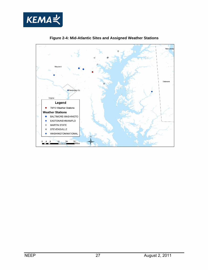
All sites associated with the sampled units were geocoded (assigned latitude and longitude)
with ArcGIS software and matched to the five closest National Oceanic and Atmospheric
Administration (NOAA) weather stations. If the closest station’s data quality was poor, the next
closest station was used. Maps were developed to show the final assignment of sites to
weather stations by weather region (Figures 2-1 through 2-6). The analysis methodology
describes the use of the nearest station actual weather data during the metered time frame to
develop unit level regression models in Section 2.3.2.

NEEP 24 August 2, 2011
Figure 2-1: Northern New England (NE-North) Sites and Assigned Weather Stations

NEEP 25 August 2, 2011
Figure 2-2: Southern New England (NE-South) Sites and Assigned Weather Stations

NEEP 26 August 2, 2011
Figure 2-3: New England – Eastern Massachusetts (NE-East Mass) Sites and Assigned
Weather Stations
NEEP 27 August 2, 2011
Figure 2-4: Mid-Atlantic Sites and Assigned Weather Stations

NEEP 28 August 2, 2011
Figure 2-5: New York Urban Coastal (NY-Urban/Coastal) Sites and
Assigned Weather Stations

NEEP 29 August 2, 2011
Figure 2-6: New York Inland (NY-Inland) Sites and Assigned Weather Stations
TMY3 Weather Stations Regional lines were determined and agreed upon to be based on state and ISO load zone/NY
Zone lines as described above. Within each weather region there are multiple sources of long
term average data for a typical meteorological year, given the large number of TMY3 stations.
The selections were made based on sample site proximity to the TMY3 station within a weather
region. It was also agreed that data from one station would be used for each weather region
rather than using any type of blended approach. A map was developed to show the units
associated with each TMY3 station.
Figure 2-7: TMY3 Weather Stations Assigned to Sites

NEEP 30 August 2, 2011

NEEP 31 August 2, 2011
2.1.2.3 Facility Type Dimension
In the facility type dimension, the project team responded to sponsor interest in facility-level
information from the study as follows: It confirmed inconsistencies exist in facility classifications
across sponsors, and it confirmed that using something as detailed as the CBECS/MECS9
classifications would create a plethora of strata that were not feasible to fill. However, the study
could record consistent designation in CBECS and another highly detailed list of types to
provide descriptive data for predominant facility types. Estimation of load shapes by facility was
outside the scope of the study.
2.1.2.4 Outside Air Intake Dimension Sponsor programs provide specific rebates for dual enthalpy economizers and it was decided by
the sponsors to exclude units with rebated dual enthalpy economizers due to the fact that the
units would affect runtime and would not offer enough results in a random sample to produce
precise results by type. The type of economizer installed on each unit in the study population
was still unknown and was not considered in the sample. The installed economizer type was
determined during the site visit providing known information on the sample that the sponsors
can use to inform their understanding of this population.
9 The U.S. Department of Energy, Energy Information Administration’s Commercial Buildings Energy
Consumption Survey (CBECS) and Manufacturing Energy Consumption Survey (MECS).

NEEP 32 August 2, 2011
2.1.2.5 Planned Sample Design
KEMA employed model-based statistical sampling (“MBSS”) to construct the sample design and
provide the framework for the subsequent analysis. MBSS techniques have been used to
create a very efficient and flexible structure for collecting data on countless energy efficiency
evaluations, demand response evaluations, and interval load data analyses, e.g., load research
and end-use metering, projects. MBSS methods provide the framework, through the use of
case weights, to allow the sponsors to analyze the resulting data based on their varying
portfolios of projects. The following sections fully describe the sample design and analysis
approach that was used in this project.
Conventional methods are documented in standard texts such as Cochran’s Sampling
Techniques.10 MBSS is grounded in theory of model-assisted survey sampling developed by
C.E. Sarndal and others.11 12 MBSS methodology has been applied in load research for more
than thirty years and in energy efficiency evaluation for more than twenty years. This fusion of
theory and practice has led to important advances in both model-based theory and interval load
data collection practice, including the use of the error ratio for preliminary sample design, the
model-based methodology for efficient stratified ratio estimation, and effective methods for
domains estimation.
As an initial assessment, we examined the error ratios associated with “large” C&I HVAC
savings for one of the regional studies that KEMA recently conducted. The error ratio
associated with the demand reduction for the forward capacity market13 (“FCM”) peak hours
was estimated to be 0.78. Other studies reviewed showed the following:
One study showed the error ratios are between .6 (single phase) and .8 (3 phase) for 60
to 80% of hours based on one set of data.
10 Sampling Techniques, by W. G. Cochran, 3rd. Ed. Wiley, 1977. 11 Model Assisted Survey Sampling, by Carl Erik Sarndal, Bengt Swensson and Jan Wretman, Springer-
Verlag, 1992. 12 Wright, R. L. (1983), “Finite population sampling with multivariate auxiliary information,” Journal of the
American Statistical Association, 78, 879-884. 13 FCM peak demand impacts are coincident with “Demand Resource On-Peak Hours” as defined by ISO New England:
Summer: June, July, and August, 1pm to 5pm, weekday non-holidays Winter: December and January, 5pm to 7pm, weekday non-holiday

NEEP 33 August 2, 2011
The error ratios for New York small C&I demand and non-demand data sets – .6 and .91
respectively.
The error ratio from a 1998 RLW study was .35 for coincident peak demand savings
Error ratios from a study where HVAC composed 50% of the projects (.92)
We recognize that there may be more variation for small C&I than for this recently observed
group. We therefore calculated the required sample given a range of error ratios near this level.
Table 2-4 presents the required unit-level (not site level) sample sizes for error ratios that range
from 0.7 to 1.4 at the 80% and 90% level of confidence and at ±10% and ±15% level of
precision. For 80/10 confidence/precision, the sample sizes range from 81 to 322 depending on
error ratio. The sample was designed to achieve minimum peak demand estimate precisions of
10% at the 90% confidence interval for the aggregate Loadshape which would require 133 to
530 sampled units depending on error ratio. The sample was designed such that total sample
would be evenly allocated by weather region and within regions proportional to the population
count for allocation by size for small and large units. This design was chosen given the
limitation of having incomplete data on existing stratum-specific estimates of error ratios that
could inform this study’s design. Through multiple meetings the Forum came to agreement on a
sample design of 45 small units and 30 large units for each of 6 weather regions for a total
sample size of 450 units which would be supplemented by some available data from the BGE
AC Profiler study.
Table 2-4: Required Sample Sizes for Considered Error Ratios and Precisions
Error Ratio
Required Sample Size
80% Confidence 90% Confidence
±10% ±15% ±10% ±15%
0.7 81 36 133 59
0.8 105 47 173 77
0.9 133 59 219 97
1 164 73 271 120
1.1 199 88 327 146
1.2 237 105 390 173
1.3 278 123 457 203
1.4 322 143 530 236

NEEP 34 August 2, 2011
The primary data collection sample design is shown below along with planned precision
estimates by stratum. The regions and size ranges were defined in the previous section. The
tracking system estimate of savings was used as a secondary variable to stratify within the large
unit strata given the large range of estimated savings within the stratum whereas many small
units had deemed savings which were uniform for units by sponsor and secondary stratification
by savings would not differentiate unit usage. There were three savings substrata in weather
regions with one very large saving unit that was placed in a certainty stratum to ensure its
inclusion in the sample.
The population used in the planned sample design in the three following tables included units
that were eliminated after further review that did not meet planning criteria. The next tables
show the precision estimates of the planned sample design and distributions including
secondary savings stratification within the large stratum. An error ratio of 1.0 was chosen for
small units and 0.6 for large units to achieve the desired precisions for peak demand estimates
as well as annual load shapes based on review of all the available information.
Table 2-5: Planned Sample Sizes and Precisions at the 90% Confidence Interval for
Primary Data Collection
The samples sizes including secondary stratification within the large stratum by savings are
shown below. The maximum unit savings within each stratum shown serves as the cut point
between strata.
ExpectedClass Sector Units Percent Units Percent Precision
Climate Unit SizeMid Atlantic Small 158 2% 45 10% ±29.7%Mid Atlantic Large 82 1% 30 7% ±15.5%NE-East Mass Small 294 4% 45 10% ±26.1%NE-East Mass Large 128 2% 30 7% ±15.8%NE-North Small 1,225 17% 45 10% ±30.1%NE-North Large 355 5% 30 7% ±18.0%NE-South Coastal Small 470 6% 45 10% ±28.4%NE-South Coastal Large 151 2% 30 7% ±16.0%NY-Inland Small 2,537 35% 45 10% ±25.5%NY-Inland Large 672 9% 30 7% ±19.3%NY-Urban/Coastal Small 917 13% 45 10% ±28.6%NY-Urban/Coastal Large 256 4% 30 7% ±17.3%
7,245 100% 450 100% ±8.7%
Sample Size
Totals
Population
NEEP 35 August 2, 2011
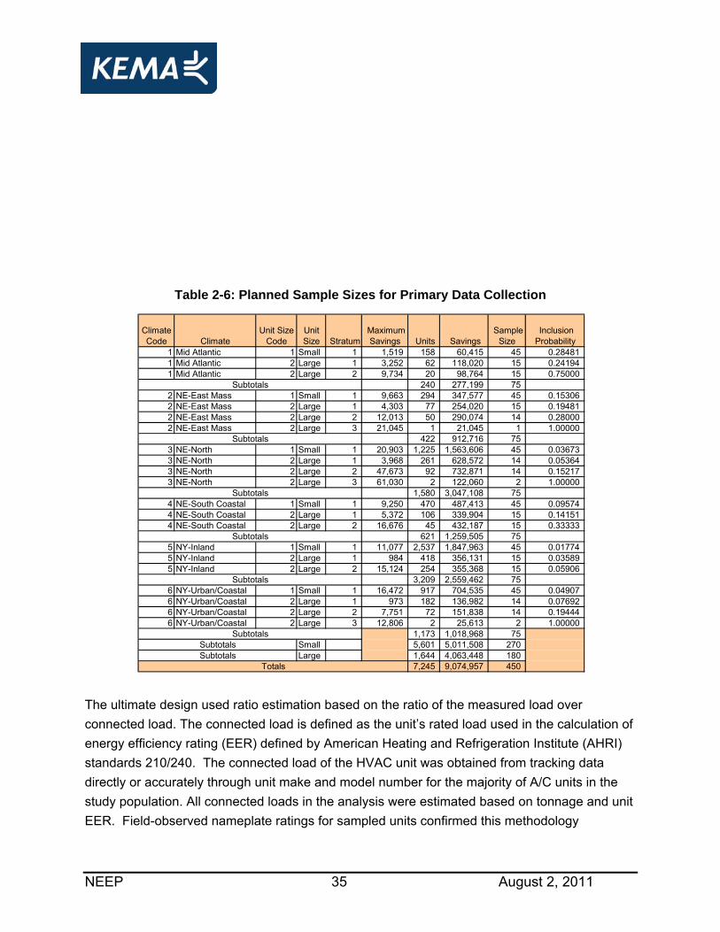
Table 2-6: Planned Sample Sizes for Primary Data Collection
The ultimate design used ratio estimation based on the ratio of the measured load over
connected load. The connected load is defined as the unit’s rated load used in the calculation of
energy efficiency rating (EER) defined by American Heating and Refrigeration Institute (AHRI)
standards 210/240. The connected load of the HVAC unit was obtained from tracking data
directly or accurately through unit make and model number for the majority of A/C units in the
study population. All connected loads in the analysis were estimated based on tonnage and unit
EER. Field-observed nameplate ratings for sampled units confirmed this methodology
Climate Code Climate
Unit Size Code
Unit Size Stratum
Maximum Savings Units Savings
Sample Size
Inclusion Probability
1 Mid Atlantic 1 Small 1 1,519 158 60,415 45 0.28481 1 Mid Atlantic 2 Large 1 3,252 62 118,020 15 0.24194 1 Mid Atlantic 2 Large 2 9,734 20 98,764 15 0.75000
240 277,199 75 2 NE-East Mass 1 Small 1 9,663 294 347,577 45 0.15306 2 NE-East Mass 2 Large 1 4,303 77 254,020 15 0.19481 2 NE-East Mass 2 Large 2 12,013 50 290,074 14 0.28000 2 NE-East Mass 2 Large 3 21,045 1 21,045 1 1.00000
422 912,716 75 3 NE-North 1 Small 1 20,903 1,225 1,563,606 45 0.03673 3 NE-North 2 Large 1 3,968 261 628,572 14 0.05364 3 NE-North 2 Large 2 47,673 92 732,871 14 0.15217 3 NE-North 2 Large 3 61,030 2 122,060 2 1.00000
1,580 3,047,108 75 4 NE-South Coastal 1 Small 1 9,250 470 487,413 45 0.09574 4 NE-South Coastal 2 Large 1 5,372 106 339,904 15 0.14151 4 NE-South Coastal 2 Large 2 16,676 45 432,187 15 0.33333
621 1,259,505 75 5 NY-Inland 1 Small 1 11,077 2,537 1,847,963 45 0.01774 5 NY-Inland 2 Large 1 984 418 356,131 15 0.03589 5 NY-Inland 2 Large 2 15,124 254 355,368 15 0.05906
3,209 2,559,462 75 6 NY-Urban/Coastal 1 Small 1 16,472 917 704,535 45 0.04907 6 NY-Urban/Coastal 2 Large 1 973 182 136,982 14 0.07692 6 NY-Urban/Coastal 2 Large 2 7,751 72 151,838 14 0.19444 6 NY-Urban/Coastal 2 Large 3 12,806 2 25,613 2 1.00000
1,173 1,018,968 75 Small 5,601 5,011,508 270 Large 1,644 4,063,448 180
7,245 9,074,957 450 Totals
Subtotals
Subtotals
Subtotals
Subtotals
Subtotals
SubtotalsSubtotalsSubtotals

NEEP 36 August 2, 2011
reasonably estimated the connected load for units even without direct tracking data or specific
model number information.
2.1.1 Achieved Population and Sample The population of study air conditioner units is presented below. It was different from the
sampling population in the previous tables due to the late exclusion of some units discovered as
older than 2007 or part of incomplete projects. The following tables describe the achieved total
population and sample including the data leveraged from previous studies. As previously
mentioned, only data from the BG&E Commercial AC Profiler study was applicable and those
data all fell under the small unit category. The BG&E study includes the power measurement of
101 units over multiple years along with the relevant weather data. Given this primary data the
study could model the units similarly to measured units and include them in the population and
sample.
Table 2-7: Population of Units and Connected Load by Region and Size Strata
Includes Leveraged Data
The final achieved sample sizes and total stratum connected loads by region and size are
shown in a series of tables. The building type and economizer distributions are presented in a
data summary following the study results. The following table describes the total sample
including the data leveraged from previous studies. As previously mentioned, only data from
the BG&E Commercial AC Profiler study was applicable and most of the data fell under the
small unit category. This study actually metered 22 units in the Mid-Atlantic small-stratum and
leveraged existing metering data on 101 units from BG&E as shown in the table. The Mid-
Atlantic-small stratum primary metering sample size was restricted to sites already recruited
after reviewing the BG&E data in more detail which determined all secondary data could be
used to fill the specific stratum. Of note, the relatively low population size of Mid-Atlantic-large
Region Small Large Total Small Large Total
Mid-Atlantic 185 71 256 1,093 1,606 2,699NE-East Mass 293 128 421 1,710 2,374 4,084NE-North 1218 352 1570 6,948 6,717 13,665NE-South Coastal 470 151 621 2,869 3,524 6,393NY- Inland 470 582 1052 2,898 7,543 10,441NY- Urban/Coastal 227 218 445 1,969 3,403 5,372
Total 2,863 1,502 4,365 17,487 25,167 42,654
Population Size "N" (Count) Population Connected Load (kW)
NEEP 37 August 2, 2011
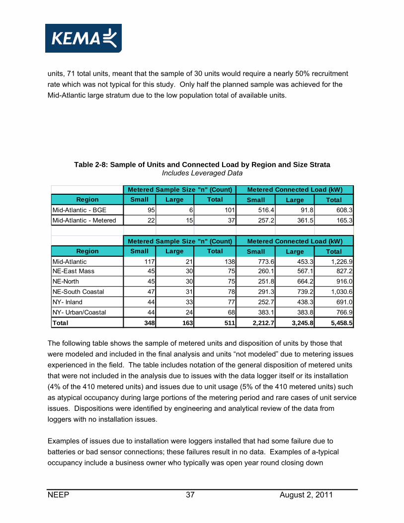
units, 71 total units, meant that the sample of 30 units would require a nearly 50% recruitment
rate which was not typical for this study. Only half the planned sample was achieved for the
Mid-Atlantic large stratum due to the low population total of available units.
Table 2-8: Sample of Units and Connected Load by Region and Size Strata Includes Leveraged Data
The following table shows the sample of metered units and disposition of units by those that
were modeled and included in the final analysis and units “not modeled” due to metering issues
experienced in the field. The table includes notation of the general disposition of metered units
that were not included in the analysis due to issues with the data logger itself or its installation
(4% of the 410 metered units) and issues due to unit usage (5% of the 410 metered units) such
as atypical occupancy during large portions of the metering period and rare cases of unit service
issues. Dispositions were identified by engineering and analytical review of the data from
loggers with no installation issues.
Examples of issues due to installation were loggers installed that had some failure due to
batteries or bad sensor connections; these failures result in no data. Examples of a-typical
occupancy include a business owner who typically was open year round closing down
Region Small Large Total Small Large Total
Mid-Atlantic - BGE 95 6 101 516.4 91.8 608.3
Mid-Atlantic - Metered 22 15 37 257.2 361.5 165.3
Region Small Large Total Small Large Total
Mid-Atlantic 117 21 138 773.6 453.3 1,226.9
NE-East Mass 45 30 75 260.1 567.1 827.2
NE-North 45 30 75 251.8 664.2 916.0
NE-South Coastal 47 31 78 291.3 739.2 1,030.6
NY- Inland 44 33 77 252.7 438.3 691.0
NY- Urban/Coastal 44 24 68 383.1 383.8 766.9
Total 348 163 511 2,212.7 3,245.8 5,458.5
Metered Connected Load (kW)Metered Sample Size "n" (Count)
Metered Sample Size "n" (Count) Metered Connected Load (kW)

NEEP 38 August 2, 2011
unexpectedly for several of the hottest weeks in the middle of the metered period. Generally if
most of the summer had typical occupancy, metered data was available for the regression, but
several weeks closed followed by sporadic and a-typical occupancy compared with the initial
data produced unreliable models with large errors relative to the actual usage pattern. An
example of unit service issues would be water getting in electrical compartments that should be
sealed which failed the logger in one case and logger and unit in another. Another case was
where the unit was serviced and operation completely changed. If an economizer was repaired
from stuck closed or a thermostat changed from constant setpoint to variable the data produced
unreliable models with large errors relative to the actual usage pattern.
The methodology for data quality control and model review are described in the following
section. The methodology for data quality control and model review are described in the
following section.
Table 2-9: Sample of Units and Connected Load Included in Analysis
Includes Leveraged Data
Region Small Large Total Small Large TotalMid-Atlantic 115 19 134 753.7 392.5 1,146.2
NE-East Mass 43 29 72 251.0 545.2 796.2
NE-North 41 28 69 236.5 638.6 875.2
NE-South Coastal 42 29 71 268.0 699.3 967.3
NY- Inland 32 32 64 179.7 419.2 599.0
NY- Urban/Coastal 41 22 63 355.6 346.3 701.9
Total 320 153 473 2,044.5 3,041.2 5,085.7Region Small Large Total Small Large Total
Mid-Atlantic 2 2 4 19.8 60.8 80.7NE-East Mass 2 1 3 9.1 21.8 31.0NE-North 4 2 6 15.2 25.6 40.8NE-South Coastal 5 2 7 23.3 39.9 63.3NY- Inland 10 1 11 56.9 19.0 75.9NY- Urban/Coastal 5 2 7 43.7 37.5 81.2
Total 28 10 38 168.1 204.7 372.8
* - 9% Total, Failure rate (failed loggers and installations) - 4%, and Other issues (HVAC unit issues and business vacancy) - 5% , Small Units Majority
Modeled
Metered Sample Size "n" (Count) Metered Connected Load (kW)
Not Modeled
*

NEEP 39 August 2, 2011
The following table does not include leveraged data, in order to show the sample distribution of
units metered by this study and ultimately included in the final analysis by Forum sponsor. Not
all Forum sponsors were able to provide sites for metering. By design and intent, the study goal
was to serve all Forum members with results that are transferable within the Forum overall
including those not able to provide sites for metering. The sample size and connected load by
sponsor are shown in Table 2-10.
Table 2-10: Metered Sample of Units and Connected Load By Sponsor
Does Not Include Leveraged Data
Table Does Not Include Leverage Data
Baltimore Gas & Electric (BGE) 25 402.2Cape Light Compact (CLC) 3 8.1
National Grid (NGRID) 105 1470.9
NSTAR 9 85.5
Northeast Utilities (NU) 27 287.6
NYSERDA 127 1300.8
PEPCO 8 135.7
Public Service New Hampshire (PSNH) 41 496.5
United Illuminating (UILL) 11 141.6
Unitil 2 27.6
Efficiency Vermont (VEIC) 14 120.8
Total 372 4477.5
Baltimore Gas & Electric (BGE) 3 58.9
Cape Light Compact (CLC)
National Grid (NGRID) 1 3.9
NSTAR 5 61.4
Northeast Utilities (NU) 2 5.7
NYSERDA 18 157.1
PEPCO 1 21.8
Public Service New Hampshire (PSNH) 5 39.4
United Illuminating (UILL) 2 23.3
Unitil
Efficiency Vermont (VEIC) 1 1.5
Total 38 372.8
Modeled
Not Modeled
*
Sample Size "n" (Count)
Connected Load (kW)Sponsor

NEEP 40 August 2, 2011
2.2 Data Collection
2.2.1 Sample Selection and Customer Recruitment Once the final sample design was approved by the NEEP project committee, KEMA drew a
random sample of C&I Unitary HVAC program units and associated sites in accordance with the
approved design and standard sampling techniques. Initial response rates by strata were used
to determine if and how many priority backup units to meter at sites with many units in the
population strata.
Recruiting methods are a vital component of studies such as this C&I Unitary HVAC Load
Shape Project. KEMA had to overcome some recruiting challenges. First, the scope of work to
be performed at a customer site was moderately intrusive; technicians required access to
electrical closets, mechanical rooms, and for the most part rooftops, all of which tend to be
access-controlled areas. Another issue of vital importance to the recruiting effort was KEMA’s
ability to prove our legitimacy to customers. Customers tend to be skeptical when a consulting
firm they are unfamiliar with contacts them “on behalf” of their utility. As such, KEMA worked
with program administrators to ensure that each sponsor had at least one point person for
customer contact. In this way, KEMA was able to provide direct references to utility contacts
during scheduling, if necessary, to alleviate customer concerns.
In addition to the aforementioned issues, recruiting and scheduling generally required detailed
planning and organization to ensure sampling quotas are achieved, optimize the data collection
process (e.g. coordinate technicians by date, time, and location), and minimize impact on the
customers.
2.2.2 Site Data Collection Inextricably linked to the success of the preceding tasks, this Site Data Collection task
represents the heart of this C&I Unitary HVAC Load Shape Project. In recognition of the
inherent challenges, KEMA assembled a senior project management team with direct
experience managing large-scale and geographically-diverse data collection efforts. Data
loggers were installed in May and early June and meters were downloaded in late September
and October of 2010.
KEMA collected data for all HVAC units specified in the final sample design and selection in
adherence to the on-site measurement protocols described in this section and used the data
collection form shown in the Appendix 6.3. KEMA recognizes the critical importance of full

NEEP 41 August 2, 2011
compliance with all state and regional measurement requirements. The power measurement
equipment complied with ISO New England and PJM Interconnection M&V protocols14. The
data collection also included unit nameplate information, outside air control type, control
settings, site building type, and data logger configuration.
While the measurement plans defined all monitoring equipment and methods, the monitoring
strategy could be summarized as rigorous, compliant, and cost-effective. This system provided
data at short intervals across a long duration on a single install: one-minute kW readings for the
entire summer. While this may seem excessive, the notable analytical advantage to such high
resolution was that it characterizes the peak observed kW of the system, avoiding any reliance
on nameplate or assumptions on equipment over-sizing. Table 2-11 below provides equipment
specifications for each of the key components of the metering suite. The metering suite
includes sensors to measure true RMS current and voltage and a recording data logger. The
current transducers and direct voltage connections of all three-phase legs are used by the
Wattnode to calculate true RMS power and transmit pulse data to the Microstation data logger.
Quantities in the table are indicated relative to the requirements of metering one sampled AC
unit.
Table 2-11: Metering Equipment Suite for one AC Unit
Temperature monitoring was not included in the KEMA work plan for reasons of cost-control
and also because hourly ambient temperature is available at low cost from proximal weather
stations.
14 New England Independent System Operator (ISO-NE) M&V Manual for Wholesale Forward Capcity
Market (FCM). www.iso-ne.com/rules_proced/isone_mnls/index.html
PJM Manual 18B:Energy Efficiency Measurement & Verification, Revision: 01
Effective Date: March 1, 2010 http://pjm.com/~/media/documents/manuals/m18b.ashx
Function /Data Point to Measure
Equipment Brand/Model
Qty Req'd
Rated Full Scale
Accuracy
Accuracy of Expected
Measurement
Planned Metering Duration
Planned Metering Interval
Power Wattnode/WNB-3D-480-P
1 ± 0.05% ± 0.45% 4+ Months
1 min
Power Onset Hobo Micro Station
1
±0.4 4+ Months
1 min
Power Magnelab Split-Core AC Current Transducer
3 ± 1% ± 1% 4+ Months
1 min

NEEP 42 August 2, 2011
Field staff began all site work by interviewing the site contact and performing a brief survey of
the space served by the incented equipment. The survey portion of the site visit followed the
progression provided below:
1. The field engineer presented the site contact with a document containing letterhead from
their local sponsor that indicates the intent of the project, stated the scope of the work to be
performed on site, and verifies the legitimacy of KEMA and L&S Energy Services. This
document contained appropriate KEMA contact information should any issues arise with the
metered equipment during the monitoring period. Contact information for the point person at
the local utility was also provided should the contact still have any concerns about the
legitimacy of the research effort.
2. Engineers explained what their on-site activities will entail and answered any customer
questions. Field engineers reiterated the details provided to the site contact during the
scheduling phone call and contained in the aforementioned document.
3. The site contact was interviewed to determine the operating schedules and set points of the
incented unitary HVAC equipment. The contact was asked if the company uses a
programmed set back schedule, or manually adjust the temperature set points to meet their
needs. If set points were manually controlled, the site contact was asked to provide
approximate on/off and hourly temperature set point schedules for the sampled AC units.
The contact was also asked to provide specific schedules for weekends, holidays, and any
other special events which may alter the normal operation of the unit. Should the contact
indicate that the HVAC equipment follows a programmed schedule, field engineers asked if
set points are ever changed, and if so, when and for what reasons. For sites with
programmed schedules, the contact was asked to show the engineer the thermostat/ EMS
interface for recording.
4. Field engineers requested that the site contact next provide access to the roof so that the
metering tasks can be completed.
a. Metering Equipment - The metering procedure uses the metering suite depicted below.

NEEP 43 August 2, 2011
Figure 2-8: Metering Equipment Picture
All on site metering activities will comply with NFPA 70E safety protocols. Furthermore,
all KEMA field staff members were required to undergo additional electrical and ladder
safety training courses annually.
b. Meter Installation - After being provided roof access by the site contact, the
following protocols will be followed to install the metering suite and verify its
correct operation.
1. Before touching any energized equipment, remove all metallic jewelry
and put on all safety gear required by the NFPA 70E standards.
2. Turn off the power by flipping the manual disconnect switch.
3. Open the unit and verify that it is completely off. This can be done by
measuring the phase voltage with a multi-meter at the unit’s primary
terminal block. Install the logger by hard wiring the voltage leads into
each phase at the terminal block with an insulated screw driver. Attach
current transducers (CTs) to the corresponding supply circuits on the
line side of the terminal block.
4. Launch the Micro Station logger for 1 minute interval metering. Turn the
unit on and verify that the logger is recording data and operating
properly. Compare the logger readings to spot measured values
collected using the procedure in section C. In the event that the logger
is not recording data or the numbers do not compare within reason to
the spot measured values, check the Wattnode status lights and consult
the field troubleshooting guide (provided with all site kits).

NEEP 44 August 2, 2011
Figure 2-9: Wattnode Status Indicator Lights
5. After correct operation has been verified, turn the unit off again and
close all HVAC unit panels. Turn the unit on and verify that it runs
before leaving the roof. This can be done by decreasing the thermostat
set point sufficiently to induce compressor operation.
c. Spot Power Measurement Check - The accuracy of all meter installations must
be verified using spot measurement checks. Spot measurements consist of
voltage, amperage, power factor, and true power readings. A minimum of three
sets of spot measurements taken 1 minute apart is required.
5. After meter equipment installation is complete, the site contact will next be asked to provide
field engineers with access to areas of the facility served by the sampled HVAC units.
Engineers will then record information regarding the space type and function (i.e. kitchen,
general office, retail, etc.) and whether any significant internal loads (server farms, kitchen
equipment, process equipment etc.) exist. For spaces with substantial internal loads, the
equipment operating schedules, energy rating and efficiency of the equipment will be
collected to inform the modeling effort. The site contact will also be asked how many people
typically occupy the space and how the occupancy schedule fluctuates throughout the day.
Engineers will also ask about and record shell characteristics data including wall
construction and roof type.
6. Before leaving the facility, field engineers will notify the site contact that a KEMA employee
will be contacting them in August to schedule a September meter retrieval date.
7. Meter removal followed all the steps of meter installation. After removing all logging
equipment from the unit, securely reinstall the panels. Turn the unit back on and make sure
it runs. If necessary, adjust the thermostat to force the unit to turn on.

NEEP 45 August 2, 2011
Data collection concluded with a visit to pick up data loggers and ask site contacts to confirm
unit operation and control strategy outside of the monitored period, especially winter months.
The responses were included in the analysis at the unit level to inform extrapolation of results to
hours outside the monitored period.
2.2.3 Secondary Data Collection Weather data for 2010 for the specified weather stations were obtained directly from the NOAA
database. TMY3 regional weather is available for free from the location referenced above. The
data collected from past studies and leveraged for load shape development was limited to that
of the BG&E Commercial AC Profiler15 project. Those load and weather data were provided by
BG&E in a format such that the data could be re-analyzed according to the specifications in the
following section. The study resulted from long term metering of units which were also subject
to demand-response load control, but having the hourly power measurements and weather data
for all hours outside the load control events was invaluable. There were four to five years of
power and weather data to model for each unit, offering good tests of modeled usage versus
actual usage across all relevant conditions. Each leveraged unit was modeled in the same
fashion as units metered according to the above data collection protocols.
BG&E’s load data were obtained from end-use meters that were installed on 101 air
conditioning units. These meters provided integrated kW demand data on a fifteen-minute
interval basis. During the summers of 2001 through 2007, BGE operated its load curtailment
program on 106 summer days. Since the focus of their research was to develop profiles of
uninterrupted air conditioner use, these days were excluded from the analysis and data set
provided. In addition, BGE identified heating usage of heat pumps which was also excluded
from the modeling in this NEEP study. The size distribution of units is shown in the table below
which also shows that 95 units went to the small stratum and 6 units went to the large stratum
within the MidAtlantic weather region.
15 Baltimore Gas and Electric Company (BGE) - Development of Commercial Load Profiler for Central Air
Conditioners and Heat Pumps. Contact Mary Straub at BGE.

NEEP 46 August 2, 2011
Table 2-12: Distribution of Leveraged Data
Stratum
Mid-Atlantic Small 1 2
Mid-Atlantic Small 1.5 6
Mid-Atlantic Small 2 6
Mid-Atlantic Small 2.5 7
Mid-Atlantic Small 3 10
Mid-Atlantic Small 3.5 2
Mid-Atlantic Small 4 8
Mid-Atlantic Small 5 41
Mid-Atlantic Small 5.5 2
Mid-Atlantic Small 6 5
Mid-Atlantic Small 7.5 4
Mid-Atlantic Small 10 2
Mid-Atlantic Large 11 2
Mid-Atlantic Large 12 1
Mid-Atlantic Large 15 3
Total 101
TonnageNumber of
Units

NEEP 47 August 2, 2011
2.3 Data Analysis The highlights of the data analysis are as follows:
Quality control performed on the hourly power measurements for all units for the cooling
season provided by the logging effort.
Modeling of each unit kW individually as a function of weather variables and other
available data.
Fitting models to normal weather series for both the normalization of the individual unit
data and the extrapolation to 8,760 load shapes; that is average kW for each hour of the
year.
The individual unit 8,760 load shapes were aggregated, hour by hour, with a ratio estimation
approach using the case weight developed in the sample design.
2.3.1 Quality Control Logging of end-use data in the field is a complicated and challenging process. The first step of
all data analysis using logged data is confirming that the data on the logger correctly reflects the
usage of that end-use. In addition to all of the checks integrated into the logging process itself,
we check each set of logger data before doing any analysis. Air conditioning data, in particular,
has a clear visual signature that allows for confirmation of the data. Unexpectedly low usage
may indicate a failed logger. Data analysts ran a series of tests on the data and worked with the
engineers who performed the data logging to confirm that all data were correct. Quality control
included checking for missing data, atypical peaking patterns, and low/high values that were
inconsistent with the unit’s size, etc. Table 2.3 in the Sample Design section describes the
number of units excluded based on the QC criteria. The following section also describes how
error analysis of the modeling results was also used to inform the engineering QC process.
As part of the quality control, the data was preprocessed to exclude times when the unit is in
fan-only mode. Fan-only mode appears as a fraction of typical unit usage but a relatively flat line
in a plot of a unit’s power draw versus time. The fan’s rated power was also factored in to
determine the correct point at which to exclude fan-only data points in the final unit level
analysis. This method excludes economizer-only and ventilation-only usage, however it does
not account for changes in outside air intake fraction during cooling operation. All fan usage
during compressor and condenser “cooling” operation was included in the analysis. Peak
coincidence factors and annual full load hours were defined to only include the cooling operation
of unitary HVAC equipment.

NEEP 48 August 2, 2011
In addition, a time series of the power draw was inspected to capture any apparent operating
schedule. The data were imported into a SAS program that extracts in different columns, the
date, hour, Weekend/Weekday, hourly average power (kW), OSA dry bulb temperature, cooling
degree hour (defined as OSA minus 65), outside air relative humidity, outside air dew point
temperature, and the temperature-humidity index (THI).
2.3.2 Unit Level Regression Modeling Approach The analysis is based on the following equation to determine unit level hourly load estimates:
Equation 2
dhdhdhhgdwdhChdh HHhgdwTHIL 3322)()( )()(
where for a particular HVAC unit;
Ldh = load on day d hour h, day= 1 to 365, hour = 1 to 8760 in kW THIdh = Temperature-humidity index on day d hour h w(d) = 0/1 dummy indicating day type of day d , Monday = 1, Sunday =7, Holiday = 8 g(h) = 0/1 dummy indicating hour group for hour h, hour group = 1 to 24 H2d = 0/1 dummy indicating that hours in day d are the second hot day in a row H3d = 0/1 dummy indicating that hours in day d are the third or more hot day in a row Ch Hh w(d) g(h) = coefficients determined by the regression 2h, 3h = hot day adjustments, a matrix of coefficients assigned to binary variables (0/1)
for hours defined for 2nd and 3rd consecutive hot days, the matrix variables are unique to each hour in each hot day
dh = residual error
Models using alternative weather variables were developed, but THI was used;
Cdh() = cooling degree-hours for day d hour h, base °FHdh = relative humidity on day d hour h
The data were filtered for the hours when the unit is on, defined as when kW > “fan only” and
other parameters (i.e. – specific hours per operating schedule) as determined necessary by the
engineer. The inputs were run in SAS multi-variable regression for kW, THI (and alternatively
CDH, RH), day-type, hour-type, and consecutive hot day adjustments. The regression used
local weather data available closest to the unit’s location with the intent that modeling the unit
this way will yield a much more accurate model that is highly sensitive to changes in
temperature and humidity inputs to THI. The estimated values from the regression represent the
, Ch, Hh, w(d), and g(h) coefficient values in the original modeling equation as shown in
Equation 1. These values were used to model the energy consumption of the unit based on THI,
NEEP 49 August 2, 2011
day type, and hour type. The 2nd and 3rd hot days, flags will be placed in the weather file to
denote whether this is the 2nd or 3rd consecutive hot day. A hot day was defined as a day when
the average dry bulb temperature for all 24 hours is greater than 80 °F. An adjustment is made
for both 2nd and 3rd hot days in the following manner: These hot day variables represent the 2h
(d,h) and 3h (d,h) terms in the original equation. Note that these terms depend on the day of the
week and hour of the day for the hour in question. For each unit level model there are 340
regression coefficients, one for each of the variables CDH, RH, day-type, and hour-type and
each consecutive hot day adjustment is 168 coefficients on the 0/1 dummy variables.
Finally, the model values are compared to the original metered data and a statistical analysis is
done to determine the mean bias error (MBE). The MBE results for the metered time frame
were used to prioritize review of the unit models by senior engineers and site staff to
supplement the QC described above under data collection. Ultimately an engineering decision
was made for each unit the model did not match to determine if poorly modeled data was a
result of the actual unit usage or if there was a measurement or other issue requiring exclusion
of the unit entirely from the aggregate load shape analysis. This error analysis can be
computed mathematically using the residual error term in the regression and the graphing
procedure for quality control also automatically calculated the mean bias error for the entire
profile and for selected time periods. Investigating the error over the various peak hours was
easier in the graphical interface. The comparative statistics are calculated for coincident data
values, i.e. data values for time periods which contain data values for both the measured (base)
and modeled (comparison) profiles. All time periods where data is missing for either the base or
comparison profile are ignored. The mean bias error, MBE, is the mean of the error or difference
between the base and comparison profiles for all pairs of coincident data points over the mean
of the coincident data points of the base profile, as shown in the equation below.
where;
bi = data value of the base profile at time period i
ci = data value of the comparison profile at time period i
n = number of coincident data points

NEEP 50 August 2, 2011
The unit level model was applied to one of six regional (TMY3) weather files to provide a
weather-normalized 8760 load shape profile for the unit. The load predicted by the model was
set to zero if the THI was less than 50°F. This decision was made based on review of the BGE
AC profiler data which included year round data collection for multiple years and usage during
off-peak metered periods. This restriction had no effect on summer peaks, only on off-peak and
annual usage. Any information collected about when the units are activated or shut down for
winter was applied when extrapolating the results. If a unit was designated as being turned on
in March and off in December then no modeled usage was calculated for January and February.
At this stage there is a unit level 8760 weather-normalized profile for each sample point.
2.3.1 Definition of Analysis Time Variables This section describes the definition of peak periods and holidays included in the analysis.
2.3.2 Peak Period Definitions
Peak period definitions vary by ISO territory. Accordingly, the Load Shape Tool and this report
include the three peak period definition options originally specified in the RFP.
ISO-NE On-Peak Period: The ISO-NE summer “Demand Resource On-Peak Hours,” are
defined as 1 PM to 5 PM on weekday non-holidays during June, July, and August. This
peak period is defined inclusive of the start instant and exclusive of the end instant,
meaning that the summer peak period therefore includes the four hours from 1:00:00 PM
to 4:59:59 PM. In practice, this means that data time stamped from 1:00 PM to 4:59 PM
will be included in the ISO-NE peak time frame for analysis purposes.
PJM On-Peak Period: The PJM On-Peak Period is structurally identical to the first,
except that it will encompass the hours from 2 PM to 6 PM instead of 1 PM to 5 PM.
ISO-NE FCM Seasonal Peak: The FCM Summer Seasonal Peak includes all non-
holiday weekday hours in June, July and August during which the ISO New England
Real-Time System Hourly Load is greater than 90% of the most recent “50/50” System
Peak Load Forecast for the summer season.
ISO-NE FCM Seasonal Peak Details
Calculation of summer seasonal peak demand reduction and related results, such as
coincidence factors is based on performance hours. Seasonal demand performance hours
for ISO-NE FCM are defined as hours when the real time ISO-NE system load meets or
NEEP 51 August 2, 2011
exceeds 90% of the predicted seasonal peak from the most recent Capacity, Electricity,
Load and Transmission Report (CELT report).
For this project KEMA needed to translate the definition of summer seasonal demand
performance hours in order to apply them to weather-normalized unit usage estimates. This
process involved several steps summarized in this section and detailed in the Appendix.
The method uses actual identified hours for 2010 and applies the actual year weather to the
ISO system loads for those hours. KEMA developed a simple regression of hourly system
load for peak hours as a function of outside temperature and THI at the various weather
regions.
As expected, the summer of 2010 contained several hours to develop a regression of
system load to weather. 2010 ISO-NE reports16 posted for the period identified the following
number of peak hours: 20 peak hours in June, 88 peak hours in July, and 53 peak hours in
August. The following equation describes the model used for each weather region.
dhdhTHIhdhThdh THITS
Where,
Sdh = ISO-NE System load for day d and hour h in megawatts (MW)
Tdh = Outdoor Dry-bulb temperature for day d and hour h in degrees oF
THIdh = ISO-NE temperature-humidity index for day d and hour h in degrees oF Th , THIh = coefficients determined by the regression
dh = residual error
The system load to weather regression differed for each weather region. The resulting equation
coefficients for each weather region are shown below along with predicted loads for an example
input. The table below has shaded headings for the regression definitions and white headings
to show an example of inputting the same weather condition in each equation.
16 ISO NE Seasonal Peak Files: http://www.iso-
ne.com/markets/othrmkts_data/fcm/reports/snlph/index.html

NEEP 52 August 2, 2011
Table 2-13: ISO-NE System Peak to Weather Regression Results
The temperature and THI from the TMY3 weather files was substituted into the equation for
each weather region to estimate system loads for weekday non-holidays in the summer months.
The loads for each hour were reviewed to determine hours with load greater than 90% of the
long term average 50/50 system peak. The derivation of the long term average is presented in
the Appendix. The load representing 90% of the long term (2005 to 2010) average 50/50
system peak was 24,472 megawatts. The raw number of hours identified for each weather
region is shown in the table below. The historic actual annual number of FCM summer
seasonal peak hours was also reviewed to provide a foundation for reviewing the results of the
regression and weather normalization process.
Table 2-14: Number of TMY3 Hours with Load Greater than 90% of Long term Average
and Comparison to Number of FCM Seasonal Peak Hours (2008-10)
The 25 hours mutually identified across all ISO-NE weather regions are specified below along
with TMY3 temperature and THI as well as predicted system load for each weather region.
Weather Region Station
Intercept
T
Temp_degF
THI
THI_degFExample Temp/THI
Predicted System Load
NE_North Boston, MA 9,919 -77 287 85/80 26,335
NE_South Concord, NH 8,845 -82 302 85/80 26,004
NE_EastMass Providence, RI 15,829 -102 234 85/80 25,937
Weather Region Station
RAW TMY3 FCM Peak
Hours
NE_North Boston, MA 172
NE_South Concord, NH 115
NE_EastMass Providence, RI 49
Year
Number of Summer Seasonal
Peak Hours
2008 29
2009 1
2010 161

NEEP 53 August 2, 2011
Table 2-15: Final Set of FCM Season Peak Hours
2.3.3 Holidays
Holidays are part of the TMY3 weather data and 2010 day types (weekday versus weekend)
and typical holidays were applied to the analysis results using a 2010 calendar. The Load
Shape Tool allows for the user selection of time periods and allows for holiday exclusion. Only
Independence Day, observed Monday July 5th in the 2010 calendar, falls within the period of the
above peak definitions so this primarily affects annual estimates or custom time period analysis
in the Load Shape Tool.
Holiday definitions vary across both ISOs and sponsor service territories. The full list of
holidays included in annual (8760 hourly) estimates has used the ISO-NE holidays, ISO-NE
Demand Response holidays, NERC holidays, and NSTAR holiday definitions to create the
Month/
Day
Hour
Ending
8760
hour
2010
Daytype
Temp.
(oF)
THI
(oF)
ISO‐NE
S_Load
(MW)
Temp.
(oF)
THI
(oF)
ISO‐NE
S_Load
(MW)
Temp.
(oF)
THI
(oF)
ISO‐NE
S_Load
(MW)
7/19 13 4789 Tuesday 78.08 73.52 25,008 87.98 77.88 25,117 89.06 82.04 26,002
7/19 14 4790 Tuesday 75.02 72.32 24,898 91.04 78.54 25,066 93.02 83.10 25,848
7/19 15 4791 Tuesday 75.02 71.99 24,805 89.96 77.68 24,894 93.02 83.10 25,848
7/19 16 4792 Tuesday 75.02 71.99 24,805 89.06 77.55 24,930 91.04 82.70 25,956
7/19 17 4793 Tuesday 73.94 71.18 24,656 87.98 77.01 24,856 87.98 80.90 25,846
7/20 13 4813 Wednesday 75.92 74.55 25,469 91.04 80.33 25,604 89.06 77.82 25,014
7/20 14 4814 Wednesday 75.02 74.10 25,409 89.96 79.46 25,432 91.04 77.90 24,830
7/20 15 4815 Wednesday 75.02 73.23 25,161 89.96 79.19 25,351 89.96 77.68 24,889
7/22 13 4861 Friday 75.92 72.44 24,865 84.02 76.82 25,123 91.94 78.99 24,996
7/22 14 4862 Friday 73.94 70.86 24,562 84.92 76.94 25,086 91.94 80.18 25,274
7/22 15 4863 Friday 75.92 72.17 24,787 84.02 76.82 25,123 89.96 79.79 25,383
7/22 16 4864 Friday 75.02 71.72 24,727 82.94 76.55 25,130 89.06 79.93 25,508
7/22 17 4865 Friday 73.04 70.41 24,503 78.98 73.97 24,679 89.06 79.34 25,369
7/26 13 4957 Tuesday 78.98 72.78 24,727 86 77.21 25,079 95 79.28 24,752
7/26 14 4958 Tuesday 82.04 73.40 24,667 84.92 76.67 25,005 95 80.52 25,043
7/26 15 4959 Tuesday 82.94 73.85 24,727 84.02 75.90 24,845 95 79.88 24,891
7/26 16 4960 Tuesday 80.06 73.65 24,892 82.04 75.83 24,987 93.92 79.34 24,875
7/27 13 4981 Wednesday 84.92 74.24 24,688 86 77.21 25,079 93.92 83.87 25,938
7/27 14 4982 Wednesday 84.02 73.52 24,551 84.92 76.67 25,005 93.02 83.10 25,848
8/15 13 5437 Monday 80.06 76.35 25,667 91.04 80.92 25,784 91.94 83.15 25,970
8/15 14 5438 Monday 82.04 77.34 25,799 91.94 81.37 25,845 91.94 82.88 25,907
8/15 15 5439 Monday 78.98 75.81 25,595 91.94 81.96 26,025 91.04 82.70 25,956
8/15 16 5440 Monday 75.92 74.55 25,469 91.94 81.69 25,943 89.96 82.49 26,015
8/15 17 5441 Monday 75.92 74.28 25,392 91.04 81.51 25,963 87.08 81.05 25,971
8/15 18 5442 Monday 77 75.09 25,541 87.98 80.31 25,851 84.02 79.19 25,847
EastMass NE‐North NE‐South

NEEP 54 August 2, 2011
following list of potential holidays and highlighted summer season holidays relevant to the peak
definitions:
New Year’s
Martin Luther King
Day
President’s Day
Good Friday
Patriot’s Day
Memorial Day
Independence Day*
Labor Day
Columbus Day
Veteran’s Day
Thanksgiving
Day after
Thanksgiving
Christmas
KEMA chose to include holidays in the Load Shape Tool by providing sponsors with a list of
holidays that can be individually selected. Each selected holiday can be selected in the “holiday”
time frame category and thus excluded from relevant time periods
2.3.4 Extrapolation Out of Sample Unit level normalized results were aggregated based on the case weights determined during the
sampling process. The analysis results were used to develop hourly case-weighted normalized
load shape data for each of the 12 strata (e.g. NY-Inland - Large). After all the unit level
modeling was done and regional weather normalization completed, each load shape profile was
pooled into 12 strata determined by 6 regions and 2 unit sizes (small <11.25 tons or large
≥11.25 tons). For each hour, the load for each stratum was calculated as the sum of the sample
loads multiplied by their case weights. For each stratum, the case-weighted sample connected
load was also calculated. The ratio of the total hourly load to the total connected load derived
from the sample data in each stratum was multiplied by the total population connected load to
estimate the total stratum hourly load. By performing this calculation for every hour, an annual
load profile was estimated. The variation in the sample customer ratios in each hour, as well as
the sample size was used to calculate the relative precision at the 90% confidence interval of
each hourly estimate. The sampling and extrapolation were performed using Load Research
Software which is specifically designed for developing estimates and precision from all 8760
hours. The software also aggregated loadshapes based on case weights to the total for region
and size strata as well as across all units. These case-weighted aggregations of the 12 strata
were not part of the tool or result tables because the Load Shape Tool was designed to use
connected load to scale estimates and to aggregate small and large unit populations within a
region. The precision of the estimate over the peak period as defined by ISO-NE and PJM as

NEEP 55 August 2, 2011
well as the precision of the annual estimate are calculations performed by the Load Shape Tool
using the stratum level data. In all strata the load shapes were near precision targets for all
peak definitions, therefore the use of cross regional load shapes was not deemed necessary for
use in the reporting or tool and combinations could be based on weighting by connected load.

NEEP 56 August 2, 2011
3 Results This section focuses on the primary results which are the annual load shape for each size and
region stratum and key parameters that can be calculated using the loadshape data. The
annual results are presented in illustrative figures and tables below. The primary results of the
study were unit-less load ratio estimates and precisions at the hourly level, which also serve as
the basis of the Load Shape Tool. The load ratio is the hourly modeled load divided by the
connected load. The average load ratio over the hours defined in a peak period is equal to the
coincidence factor. The sum of load ratios over a year is equal to the equivalent full load
cooling hours. Results (demand and annual energy) extrapolated to the population in physical
units of kW and kWh are available through the Load Shape Tool by entering population
connected loads.
The usage estimates generated from this study show some usage occurring outside the
monitored period of May to September. Various steps were taken to explain the non-summer
usage. Interviews with facility staff were conducted during the logger pickup visit to determine
seasonal operation outside the metered period. While not all site contacts could provide
detailed schedule information, many responses were that the units would operate if necessary
in winter. Long term metered data that was leveraged for this study, provided by BG&E,
showed actual metered non-summer usage consistent with the modeled usage of units
(restricted to THI > 50) only monitored by this study in summer 2010 and extrapolated to the
same weather data recorded in the long term metered data set. An extensive analysis was
beyond the scope of this study, but a reasonable effort was made to validate the results. For
large units, the internal building loads such as lighting and occupants are such that the cooling
systems were used more consistently across temperature ranges than small units. Although not
presented in the report, data in the Load Shape Tool show the relative precision and error ratios
for winter hours were much higher than the hours included in peak definitions where there is
more likely coincident usage across a region. The extreme error ratios were a result of many
units having zero usage with one or a few units having some sporadic usage. The 8,760
profiles in section 3.2 show the limited usage in winter months, but rather extensive off-peak
summer usage.

NEEP 57 August 2, 2011
3.1 Normalized Study Results and Basis of Load Shape Tool
The following tables present the annual usage and coincident peak estimates and relative
precisions based on the developed load shapes. The data are normalized by connected load
such that the results are unit-less, coincidence and annual load factors, except for effective full
load cooling hours. All tables include estimated factors or full load hours. Each estimated factor
is presented with the relative precision of each estimate at the 80% and 90% two-tail confidence
intervals, abbreviated respectively as “RP @ 80%CI” and “RP @ 90%CI. As a reminder,
relative precision at the 80% two-tail interval is equivalent to that of the 90% one-tail.
The following table presents the annual load factor and effective full load hours for the regional
totals and the relative precisions of the estimates. The annual load factor represents the
fraction of hourly regional loadshape divided by connected load for all 8,760 hours or more
simply, the fraction of effective full load cooling hours over 8,760.
The relative precisions of the two estimates are identical given there is only division by a
constant. The precisions were much lower than the planned precisions from the sample design
for peak demand factors. As shown below, precisions for all of the load-weighted regional totals
are less than 23%. The precision calculations are based on aggregation of the hourly estimates
and hourly error terms and can be replicated in detail in the Load Shape Tool.
Table 3-1: Annual Load Factor and EFLH Estimate by Region Totals
760,8
)(
)(8760
1
EFLHFactorAnnualLoad
kWLoadConnected
kWLoadHourlyEstimatedEFLH
h
Total
RegionEstimated
RatioRP @ 80%CI
RP @ 90%CI
Annual Estimate
RP @ 80%CI
RP @ 90%CI
Mid-Atlantic 0.1707 ±9.78% ±12.55% 1,495 ±9.78% ±12.55%
NE-East Mass 0.1339 ±10.12% ±12.99% 1,173 ±10.12% ±12.99%
NE-North 0.0862 ±13.14% ±16.87% 755 ±13.14% ±16.87%
NE-South Coastal 0.0976 ±11.44% ±14.69% 855 ±11.44% ±14.69%
NY- Inland 0.1087 ±13.58% ±17.43% 952 ±13.58% ±17.43%
NY- Urban/Coastal 0.1704 ±10.69% ±13.72% 1,492 ±10.69% ±13.72%
Annual Load Factor (EFLH/8760)
EFLH = Effective Full Load Cooling Hours
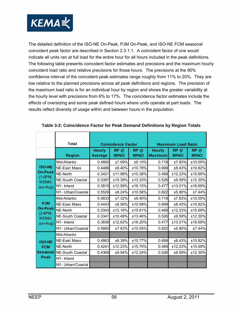
NEEP 58 August 2, 2011
The detailed definition of the ISO-NE On-Peak, PJM On-Peak, and ISO-NE FCM seasonal
coincident peak factor are described in Section 2.3.1.1. A coincident factor of one would
indicate all units ran at full load for the entire hour for all hours included in the peak definitions.
The following table presents coincident factor estimates and precisions and the maximum hourly
coincident load ratio and relative precisions for those hours. The precisions at the 90%
confidence interval of the coincident peak estimates range roughly from 11% to 20%. They are
low relative to the planned precisions across all peak definitions and regions. The precision of
the maximum load ratio is for an individual hour by region and shows the greater variability at
the hourly level with precisions from 6% to 17%. The coincidence factor estimates include the
effects of oversizing and some peak defined hours where units operate at part loads. The
results reflect diversity of usage within and between hours in the population.
Table 3-2: Coincidence Factor for Peak Demand Definitions by Region Totals
Total
RegionHourly
AverageRP @ 80%CI
RP @ 90%CI
Hourly Maximum
RP @ 80%CI
RP @ 90%CI
Mid-Atlantic 0.4892 ±7.09% ±9.10% 0.718 ±7.83% ±10.05%
NE-East Mass 0.4488 ±8.40% ±10.78% 0.699 ±8.43% ±10.82%
NE-North 0.3421 ±11.98% ±15.38% 0.469 ±12.23% ±15.69%
NE-South Coastal 0.3397 ±10.39% ±13.33% 0.526 ±9.59% ±12.30%
NY- Inland 0.3815 ±12.59% ±16.15% 0.477 ±13.01% ±16.69%
NY- Urban/Coastal 0.5529 ±8.24% ±10.58% 0.822 ±5.80% ±7.44%
Mid-Atlantic 0.4833 ±7.32% ±9.40% 0.718 ±7.83% ±10.05%
NE-East Mass 0.4443 ±8.56% ±10.99% 0.699 ±8.43% ±10.82%
NE-North 0.3343 ±12.16% ±15.61% 0.469 ±12.23% ±15.69%
NE-South Coastal 0.3341 ±10.49% ±13.46% 0.526 ±9.59% ±12.30%
NY- Inland 0.3836 ±12.62% ±16.20% 0.477 ±13.01% ±16.69%
NY- Urban/Coastal 0.5665 ±7.83% ±10.05% 0.822 ±5.80% ±7.44%
Mid-Atlantic
NE-East Mass 0.4863 ±8.39% ±10.77% 0.699 ±8.43% ±10.82%
NE-North 0.4241 ±12.23% ±15.70% 0.469 ±12.23% ±15.69%
NE-South Coastal 0.4369 ±9.54% ±12.24% 0.526 ±9.59% ±12.30%
NY- Inland
NY- Urban/Coastal
ISO-NE FCM
Seasonal Peak
ISO-NEOn-Peak (1-5PM, WDNH, Jun-Aug)
Maximum Load Ratio
PJMOn-Peak (2-6PM, WDNH, Jun-Aug)
Coincidence Factor

NEEP 59 August 2, 2011
The following table presents the annual load factor and effective full load hours for the small
units for each region and the relative precisions of the estimates. The precisions were generally
near the planned precisions for peak demand factors with the regional range at the 90%
confidence interval of 11% to 33%. The precision calculations are based on aggregation of the
hourly estimates and hourly error terms and can be replicated in detail in the Load Shape Tool.
Table 3-3: Load Ratio Estimate by Region Small Units
The following table presents small unit coincidence factor estimates and precisions and
maximum hourly coincident load ratios and associated relative precisions. The precisions of the
coincident peak estimates were on the order of 10 to 29% across the range of definitions and
regions. The precisions of the maximum load ratio at the hourly level were from 6 to 29%. The
coincidence factor estimates include the effects of oversizing and some peak defined hours
where units operate at part loads. The results reflect diversity of usage within and between
hours in the population.
SMALL units (<11.25 TONS)
Small Units
RegionEstimated
RatioRP @ 80%CI
RP @ 90%CI
Annual Estimate
RP @ 80%CI
RP @ 90%CI
Mid-Atlantic 0.1157 ±6.79% ±8.72% 1,014 ±6.79% ±8.72%
NE-East Mass 0.1261 ±14.78% ±18.97% 1,104 ±14.78% ±18.97%
NE-North 0.0946 ±19.18% ±24.62% 829 ±19.18% ±24.62%
NE-South Coastal 0.1064 ±14.98% ±19.22% 932 ±14.98% ±19.22%
NY- Inland 0.0752 ±25.39% ±32.59% 659 ±25.39% ±32.59%
NY- Urban/Coastal 0.1375 ±8.27% ±10.62% 1,204 ±8.27% ±10.62%
Annual Load Factor (EFLH/8760) EFLH
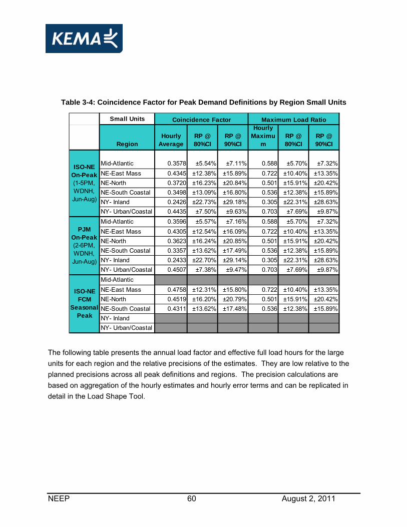
NEEP 60 August 2, 2011
Table 3-4: Coincidence Factor for Peak Demand Definitions by Region Small Units
The following table presents the annual load factor and effective full load hours for the large
units for each region and the relative precisions of the estimates. They are low relative to the
planned precisions across all peak definitions and regions. The precision calculations are
based on aggregation of the hourly estimates and hourly error terms and can be replicated in
detail in the Load Shape Tool.
Small Units
RegionHourly
AverageRP @ 80%CI
RP @ 90%CI
Hourly Maximu
mRP @ 80%CI
RP @ 90%CI
Mid-Atlantic 0.3578 ±5.54% ±7.11% 0.588 ±5.70% ±7.32%
NE-East Mass 0.4345 ±12.38% ±15.89% 0.722 ±10.40% ±13.35%
NE-North 0.3720 ±16.23% ±20.84% 0.501 ±15.91% ±20.42%
NE-South Coastal 0.3498 ±13.09% ±16.80% 0.536 ±12.38% ±15.89%
NY- Inland 0.2426 ±22.73% ±29.18% 0.305 ±22.31% ±28.63%
NY- Urban/Coastal 0.4435 ±7.50% ±9.63% 0.703 ±7.69% ±9.87%
Mid-Atlantic 0.3596 ±5.57% ±7.16% 0.588 ±5.70% ±7.32%
NE-East Mass 0.4305 ±12.54% ±16.09% 0.722 ±10.40% ±13.35%
NE-North 0.3623 ±16.24% ±20.85% 0.501 ±15.91% ±20.42%
NE-South Coastal 0.3357 ±13.62% ±17.49% 0.536 ±12.38% ±15.89%
NY- Inland 0.2433 ±22.70% ±29.14% 0.305 ±22.31% ±28.63%
NY- Urban/Coastal 0.4507 ±7.38% ±9.47% 0.703 ±7.69% ±9.87%
Mid-Atlantic
NE-East Mass 0.4758 ±12.31% ±15.80% 0.722 ±10.40% ±13.35%
NE-North 0.4519 ±16.20% ±20.79% 0.501 ±15.91% ±20.42%
NE-South Coastal 0.4311 ±13.62% ±17.48% 0.536 ±12.38% ±15.89%
NY- Inland
NY- Urban/Coastal
ISO-NE FCM
Seasonal Peak
PJMOn-Peak (2-6PM, WDNH, Jun-Aug)
ISO-NEOn-Peak (1-5PM, WDNH, Jun-Aug)
Maximum Load RatioCoincidence Factor

NEEP 61 August 2, 2011
Table 3-5: Load Ratio Estimate by Region Large Units
The following table presents large unit coincidence factor estimates and precisions and
maximum hourly coincident load ratio and relative precisions for those hours. The precisions of
the coincident peak estimates were on the order of 11 to 20% across the range of definitions
and regions. The precisions of the maximum load ratio represent an individual hour by region
and shows greater variability at the hourly level with precisions from 9 to 24%. The coincidence
factor estimates include the effects of oversizing and some peak defined hours where units
operate at part loads. The results reflect diversity of usage within and between hours in the
population.
LARGE units (≥ 11.25 TONS)
Large Units
RegionEstimated
RatioRP @ 80%CI
RP @ 90%CI
Annual Estimate
RP @ 80%CI
RP @ 90%CI
Mid-Atlantic 0.2081 ±13.24% ±16.99% 1,823 ±13.24% ±16.99%
NE-East Mass 0.1396 ±13.67% ±17.54% 1,223 ±13.67% ±17.54%
NE-North 0.0775 ±17.26% ±22.15% 679 ±17.26% ±22.15%
NE-South Coastal 0.0905 ±17.21% ±22.09% 793 ±17.21% ±22.09%
NY- Inland 0.1215 ±15.69% ±20.13% 1,065 ±15.69% ±20.13%
NY- Urban/Coastal 0.1894 ±14.78% ±18.97% 1,659 ±14.78% ±18.97%
EFLHAnnual Load Factor
(EFLH/8760)

NEEP 62 August 2, 2011
Table 3-6: Coincidence Factor for Peak Demand Definitions by Region Large Units
Large Units
RegionHourly
AverageRP @ 80%CI
RP @ 90%CI
Hourly Maximum
RP @ 80%CI
RP @ 90%CI
Mid-Atlantic 0.5787 ±9.80% ±12.58% 0.874 ±10.17% ±13.05%
NE-East Mass 0.4591 ±11.33% ±14.55% 0.683 ±12.56% ±16.12%
NE-North 0.3113 ±17.75% ±22.78% 0.438 ±18.65% ±23.93%
NE-South Coastal 0.3314 ±15.70% ±20.16% 0.543 ±14.43% ±18.51%
NY- Inland 0.4348 ±14.49% ±18.59% 0.545 ±15.04% ±19.30%
NY- Urban/Coastal 0.6162 ±11.25% ±14.44% 0.893 ±8.58% ±11.01%
Mid-Atlantic 0.5674 ±10.20% ±13.10% 0.874 ±10.17% ±13.05%
NE-East Mass 0.4543 ±11.58% ±14.87% 0.683 ±12.56% ±16.12%
NE-North 0.3054 ±18.35% ±23.55% 0.438 ±18.65% ±23.93%
NE-South Coastal 0.3328 ±15.48% ±19.87% 0.543 ±14.43% ±18.51%
NY- Inland 0.4375 ±14.53% ±18.64% 0.545 ±15.04% ±19.30%
NY- Urban/Coastal 0.6335 ±10.62% ±13.64% 0.893 ±8.58% ±11.01%
Mid-Atlantic
NE-East Mass 0.4940 ±11.36% ±14.58% 0.683 ±12.56% ±16.12%
NE-North 0.3953 ±18.60% ±23.87% 0.438 ±18.65% ±23.93%
NE-South Coastal 0.4416 ±13.27% ±17.03% 0.543 ±14.43% ±18.51%
NY- Inland
NY- Urban/Coastal
ISO-NE FCM
Seasonal Peak
Coincidence Factor Maximum Load Ratio
ISO-NEOn-Peak (1-5PM, WDNH, Jun-Aug)
PJMOn-Peak (2-6PM, WDNH, Jun-Aug)

NEEP 63 August 2, 2011
3.2 Additional Results
The primary results presented in the previous section provide a summary of the load shape
data. This section provides additional figures to illustrate other aspects of the load shapes
developed.
The first set of figures provides a graphical representation of the annual load shapes. The
format is an energy print which displays the hours of the day on the x-axis and the day of the
year on the y-axis with color coding to show hourly load ratios with black representing zero and
lighter colors representing increasing regional cooling demand. There are energy prints for
each region representing the total load shape across small and large units as well as the
separate regional profiles for small and large units. Note that the y-axis provides the first letter
of the month and the x-axis provides the hours zero through 24. The plots are of load ratio so
there are no physical units. The maximums correspond to the maximum hourly demands
shown in the section 3.1 tables.

NEEP 64 August 2, 2011
Figure 3-1: Annual Small Unit Load Shapes Shown as Energy Prints

NEEP 65 August 2, 2011
Figure 3-2: Annual Large Unit Load Shapes Shown as Energy Prints

NEEP 66 August 2, 2011
3.3 Data Summary
This section of the report presents other results that may be gleaned from the data collected,
but were not primary study objectives and are provided in response to sponsor interests. The
data summary provides insight into the average performance of sample units based on several
parameters which were inconsistent across sponsor data and thus cannot be extrapolated to the
population. Precisions were thus not calculated as the values would not be consistent with the
population weighted results developed and used in the Load Shape Tool. The sample size
distributions are presented, followed by annual and peak averages for each cross tabulation of
the sample. The data are presented in two sections; Building Type Summary and Economizer
Summary. There is intentionally little discussion of the data summary tables as they are
provided to share information on secondary study objectives.
The following table shows the sample size and total connected load in the metered sample by
building type and size of HVAC unit. Recall that connected loads are based on EER and
tonnage. The data are un-weighted by sample weights for the sample of units characterized by
building type. The sample (including leveraged units) was dominated by retail and office types;
smaller samples exist for other building types.
Table 3-7: Sample of Units and Metered Connected Load by Building Type and Size
Small Large Total Small Large TotalEducation 11 6 17 78.2 150.7 228.9
Food Sales 14 3 17 111.6 94.6 206.2Food Service 9 2 11 73.1 33.5 106.7
Health Care-inpatient 2 0 2 30.0 0.0 30.0Health Care-outpatient 1 2 3 2.1 78.1 80.1
Lodging 6 1 7 20.6 8.6 29.3
Mercantile (Retail) 111 95 206 859.3 1,793.6 2,652.9
Mercantile (Mall) 3 21 24 37.0 371.1 408.1Office 96 11 107 514.9 259.7 774.6Other 49 14 63 224.0 278.1 502.1
Public Assembly 3 1 4 14.4 23.5 37.9Public Order and Safety 3 1 4 14.8 21.2 36.0
Religious Worship 31 0 31 158.4 0.0 158.4
Service 1 5 6 3.6 104.5 108.1
Warehouse and Storage 8 1 9 70.6 28.6 99.2
Total 348 163 511 2,212.7 3,245.9 5,458.5
CBECS Building TypeMetered Sample Size "n" (Count) Metered Connected Load (kW)

NEEP 67 August 2, 2011
The following table shows the average load factor and effective full load cooling hour averages
for the sample and indicates where sample sizes are less than 10. The table is followed by
analysis results of the standard error for each estimate which further supports or advises
caution of the use of these sample un-weighted averages. All results are inherently weighted by
connected load of the units in the cross-tabulation.
Table 3-8: Annual Energy Estimate by Building Type
Sample n > 10
Sample n < 10
CBECS Building Type Annual Load Factor
(EFLH/8,760) EFLH = Effective Full Load
Cooling Hours
Small Large Total Small Large Total
Education 0.119 0.043 0.060 1,044 376 524
Food Sales 0.169 0.096 0.127 1,477 840 1,116
Food Service 0.175 0.198 0.192 1,536 1,733 1,678
Health Care - Inpatient 0.134 0.000 0.134 1,178 - 1,178
Health Care - Outpatient 0.097 0.030 0.032 848 261 276
Lodging 0.082 0.134 0.098 721 1,175 855
Mercantile (Retail) 0.113 0.123 0.120 992 1,073 1,048
Mercantile (Mall) 0.084 0.110 0.108 734 967 945
Office 0.083 0.101 0.091 726 886 799
Other 0.089 0.131 0.115 780 1,147 1,006
Public Assembly 0.032 0.104 0.076 281 908 670
Public Order and Safety 0.131 0.021 0.066 1,144 187 579
Religious Worship 0.040 0.000 0.040 351 - 351
Service 0.067 0.185 0.181 591 1,622 1,588
Warehouse and Storage 0.056 0.362 0.263 489 3,174 2,307

NEEP 68 August 2, 2011
Annual Load Percent Standard Error / Mean
The detailed definition of the ISO-NE On-Peak, PJM On-Peak, and ISO-NE FCM seasonal
coincident peak factor are described in Section 2.3.1.1. A coincidence factor of one would
indicate all units ran at full load for the entire hour for all hours included in the peak definitions.
The following table presents coincidence factor estimates and indication of sample sizes less
than 10 for all peak definitions and building types. The table is followed by analysis results of the
standard error for each ISO-NE On-peak estimate which further supports or advises caution of
the use of these un-weighted sample averages.
Table 3-9: Coincidence Factor Estimate by Building Type
Does Not Include Leverage Data
CBECS Building Type Coincidence Factor
Small Large Total
ISO-NE On-Peak (1-5PM, WDNH,
Jun-Aug)
Education 0.388 0.167 0.238 Food Sales 0.547 0.413 0.553
Food Service 0.682 0.650 0.812 Health Care-inpatient 0.586 0.000 0.948
Health Care-outpatient 0.463 0.122 0.142 Lodging 0.246 0.297 0.343
Mercantile (Retail) 0.401 0.461 0.446 Mercantile (Mall) 0.409 0.434 0.448
Education
Food SalesFood Service
Health Care-inpatient
Health Care-outpatient
Lodging
Mercantile (Retail)
Mercantile (Mall)
Office
Other
Public Assembly
Public Order and Safety
Religious WorshipService
Warehouse and Storage
27%63%
40%
15% 16%
67%
78%
CBECS Building TypeSmall Standard Error [Standard Dev / n^.5 ]
Large Standard Error [Standard Dev / n^.5 ]
13%13%
30%
11% 8%
9%
35%
10%6%
26% 34%
59%
19% 20%

NEEP 69 August 2, 2011
CBECS Building Type
Coincidence Factor
Small Large Total Office 0.318 0.385 0.357 Other 0.345 0.465 0.437
Public Assembly 0.135 0.386 0.343 Public Order and Safety 0.438 0.152 0.396
Religious Worship 0.123 0.000 0.149 Service 0.290 0.568 0.568
Warehouse and Storage 0.187 0.901 0.714
PJM On-Peak (2-6PM, WDNH,
Jun-Aug)
Education 0.373 0.151 0.223 Food Sales 0.550 0.425 0.519
Food Service 0.675 0.664 0.803 Health Care-inpatient 0.535 0.000 0.843
Health Care-outpatient 0.449 0.111 0.132 Lodging 0.269 0.292 0.360
Mercantile (Retail) 0.405 0.466 0.451 Mercantile (Mall) 0.394 0.435 0.447
Office 0.308 0.370 0.344 Other 0.341 0.454 0.429
Public Assembly 0.139 0.370 0.338 Public Order and Safety 0.440 0.129 0.384
Religious Worship 0.126 0.000 0.153 Service 0.263 0.586 0.584
Warehouse and Storage 0.180 0.908 0.714
ISO-NE FCM
Seasonal Peak
Education 0.453 0.204 0.285 Food Sales 0.557 0.479 0.556
Food Service 0.708 0.654 0.811 Health Care-inpatient 0.622 0.984
Health Care-outpatient 0.494 0.000 0.025 Lodging 0.041 0.000 0.044
Mercantile (Retail) 0.121 0.221 0.193 Mercantile (Mall) 0.461 0.459 0.476
Office 0.277 0.158 0.230 Other 0.238 0.131 0.186
Public Assembly 0.019 0.352 0.233 Public Order and Safety 0.524 0.232 0.489
Religious Worship 0.000 0.002 Service 0.419 0.407 0.422
Warehouse and Storage 0.054 0.930 0.668

NEEP 70 August 2, 2011
ISO-NE On-Peak Percent Standard Error / Mean
Recall that units with rebated economizers were excluded from the study population such that
all economizers present in the study represent the random occurrence of unit outside air
economizer (dry bulb or enthalpy) use for cooling. The following table shows the sample size
and total connected load for each of the simple averages presented by economizer type.
The data are sample-unweighted results for the sample of units characterized by outside air
intake type. The sample (assuming no economizers on leveraged units) had a very low
saturation of dual temperature and enthalpy economizers. The single temperature and enthalpy
economizers tended to be on small units and a large number of units had unknown outside air
controls. All “don’t know” units had non-fixed outside air intake and many were believed to be
single temperature/enthalpy but there was no definitive confirmation for some economizers from
third party manufacturers (an economizer not specified by the AC manufacturer as associated
with the unit). Note that the table groups dual temperature and dual enthalpy units under
“differential temperature” as well as single temperature and single enthalpy under “single
temperature” units given the sample sizes and limited information for some economizer brands.
Education
Food SalesFood Service
Health Care-inpatient
Health Care-outpatient
Lodging
Mercantile (Retail)
Mercantile (Mall)
Office
Other
Public Assembly
Public Order and Safety
Religious WorshipService
Warehouse and Storage 67%
65%40%
70%
Small Standard Error [Standard Dev / n^.5 ]
Large Standard Error [Standard Dev / n^.5 ]
12%
17%
9%
19%
61%
28%
14% 11%
18%
5%
29% 42%
11%37%
CBECS Building Type
55%
77% 23%

NEEP 71 August 2, 2011
Table 3-10: Sample of Units and Connected Load by Economizer Type and Size
The following table shows the average load factor and effective full load cooling hour averages
for the sample and indicates where sample sizes are less than 10. The table is followed by
analysis results of the standard error for each estimate which further supports or advises
caution of the use of these un-weighted sample averages. Large units show an expected trend
while small units showed potential that single temperature economizers may be malfunctioning
and increasing run hours over no economizer.
Table 3-11: Annual Energy Estimate by Economizer Type with Standard Error
Sample n > 10 Annual Load Factor (EFLH/8,760)
EFLH = Effective Full Load Cooling Hours Sample n < 10
Economizer Small Large Total Small Large Total Differential Temperature 0.093 0.087 0.089 816 765 775
Single Temperature 0.137 0.106 0.125 1,199 929 1,092 Fixed 0.041 0.142 0.062 358 1,244 545 None 0.089 0.136 0.116 782 1,191 1,013
Don't Know 0.097 0.115 0.110 851 1,006 964
Mean Annual Load Percent Standard Error / Mean
EconomizerSmall Large Total Small Large Total
Differential Temperature 17 18 35 112.3 429.4 541.7Single Temperature 66 16 82 527.8 347.4 875.2
Fixed 12 1 13 46.8 12.5 59.3
None 186 69 255 1,032.4 1,120.1 2,152.4
Don't Know 61 65 126 493.4 1,336.5 1,829.9
Total 348 163 511 2,212.7 3,245.9 5,458.5
Metered Sample Size "n" (Count) Metered Connected Load (kW)
Economizer
Differential Temperature
Single Temperature
Fixed
None
Don't Know
22%
8% 5%
7% 9%
19% 31%
7% 18%
Small Standard Error [Standard Dev / n^.5 ]
Large Standard Error [Standard Dev / n^.5 ]

NEEP 72 August 2, 2011
The detailed definition of the ISO-NE On-Peak, PJM On-Peak, and ISO-NE FCM seasonal
coincident peak factor are described in Section 2.3.1.1. A coincidence factor of one would
indicate all units ran at full load for the entire hour for all hours included in the peak definitions.
The following table presents coincidence factor estimates and indication of sample sizes less
than 10 for all peak definitions and economizer types. The table is followed by analysis results
of the standard error for each estimate which further supports or advises caution of the use of
these un-weighted sample averages.
Table 3-12: Coincidence Factor Estimate by Economizer Type with Standard Error
Sample n > 10 Sample n < 10
Coincidence Factor
Economizer Small Large Total
ISO-NE On-Peak (1-5PM WDNH,
Jun-Aug)
Differential Temperature 0.357 0.310 0.320
Single Temperature 0.429 0.409 0.421
Fixed 0.151 0.447 0.214
None 0.306 0.423 0.367
Don't Know 0.322 0.398 0.377
Total 0.338 0.396 0.373
PJM On-Peak (2-
6PM, WDNH,
Jun-Aug)
Differential Temperature 0.355 0.309 0.319
Single Temperature 0.439 0.410 0.428
Fixed 0.140 0.445 0.204
None 0.307 0.434 0.373
Don't Know 0.319 0.399 0.377
Total 0.340 0.400 0.376
ISO-NE FCM
Seasonal Peak
Differential Temperature 0.401 0.196 0.238
Single Temperature 0.213 0.161 0.193
Fixed 0.204 0.661 0.300
None 0.062 0.264 0.167
Don't Know 0.212 0.270 0.255
Total 0.152 0.248 0.209
ISO-NE On-Peak Percent Standard Error / Mean
Economizer
Differential Temperature
Single Temperature
Fixed
None
Don't Know
15% 5%
1% 9%
19% 32%
7% 18%
22%
Small Standard Error [Standard Dev / n^.5 ]
Large Standard Error [Standard Dev / n^.5 ]

NEEP 73 August 2, 2011
4 Description of HVAC Load Shape Tool and Final Data Set The following information is also described on the ReadMe worksheet of the C&I Unitary HVAC
Load Shape Tool.
4.1 Overview of HVAC Load Shape Tool The C&I Unitary HVAC Load Shape Tool (LST) was designed to calculate the peak and annual
energy savings from the installation of typical high efficiency unitary direct expansion (DX)
systems installed at commercial and industrial sites based on a specified load reduction. The
tool also outputs the energy load shapes in EEI (Edison Electric Institute) format. The following
documents the inputs, outputs, and instructions for how to use the tool. The LST is intended to
represent single air conditioning units or multiple units so long as the units are greater than 1
ton and less than 100 ton and are unitary DX systems
The above report describes the methodology and results of the study which provide the
underlying data of the LST. The tool includes a summary of the total number of units and total
connected load that were sampled from in the metering study are listed in primary input and
output page. Metered data and actual weather data were used to develop a linear regression in
SAS and models were then run using TMY3 typical weather data for the region. The LST
includes active calculations of precision based on the underlying study results. There is a
specific worksheet in the tool with the extrapolated load ratios (ratio of modeled kW / connected
load kW) and precision (90% two tail) for each hour for each strata. The coincidence factor in
the LST is equal to the average of the hourly load ratios for the defined period in the peak
definition. The Load Shape Tool also allows user specification of time periods and/or
temperature thresholds for user defined analyses.
4.2 Instructions for obtaining and using HVAC Load Shape Tool The C&I Unitary HVAC Load Shape Tool can be obtained from NEEP through their website
www.neep.org. The tool instructions are provided in this section to illustrate inputs and outputs
of the tool.
4.3 Step-By-Step Instructions 1. Select a peak definition and region
a) Appropriate hours and day types will be automatically included
b) The listed holidays will be automatically excluded from coincidence factor (but not
annual) analysis unless the user specifies

NEEP 74 August 2, 2011
2. Specify the connected load reduction (CLR) in kW for the population or by size classification.
a) Defaults for each region are shown below the CLR inputs
b) If 0% is entered for small and large then defaults will be used
c) Enter percentage of total CLR for small and large or enter 100% in correct size range
and 0 in the other to represent one unit.
3. Choose a custom time frame to include in the analysis
a) Check the months you would like to include in your analysis
b) Check the days you would like to include in your analysis
c) Check the hours of the day you would like to include in your analysis. (i.e.- for hours
10 AM – 11 AM, check 11 AM)
d) Check the Holidays to include in the analysis. If not checked, energy savings, if any
for these holidays, will not show up in the results.
e) Enter high and low outdoor temperatures and those not meeting the criteria will be
excluded in the results.
f) Enter high and low THI and those not meeting the criteria will be excluded in the
results.
4. The results sections in orange color will provide you with the annual 8760 kWh savings, the
selected period kWh savings, the selected period demand savings averaged over the specified
hours, and the demand savings per the peak definition. It also has the selected period kWh
savings as a percent of the 8760 savings, the number of hours included in the period of interest
and the precision at 80% and 90% confidence. These values are also broken out into unit sizes.
5. Switch over to the labeled tab to view the load shape in EEI format.
4.4 Overview of Data Set Available to Sponsors The load shape tool and report provide the study methodology and primary results. The study
produced a large amount of data to arrive at the final results that were not presented in either
format. The sponsors were provided a data set including all metered data, site observations,
weather data, and unit level analysis result. The data were formatted and analyzed in SAS and
thus the data set is best replicated in the available SAS format. The data was also provided in a
comma-delimited format to allow for review in any analysis format.

NEEP 75 August 2, 2011
5 Appendix
5.1 C&I Unitary HVAC Data Request Submitted to Forum Members The following information was requested for each applicable Forum member program:
a) Tracking savings estimates on a per unit/site basis –
For any program, we request that gross tracking savings (kWh and coincident kW)
be provided individually for each HVAC unit in the population. In the event that unit
level tracking data was unavailable, project level savings information should be
provided at a minimum. For programs with savings specified at the project level, the
scope of project designation should be clearly indicated (i.e., whether an individual
building, multiple buildings, or a specific customer constitutes one project).
Documentation indicating computational inputs and procedures used to calculate
savings for each measure should be provided. If deemed savings were used to
calculate savings, KEMA requires the appropriate work papers indicating the
theoretical basis of the deemed values. This information was used to evaluate the
consistency of measure savings calculations across different Forum members’
programs. It will therefore indicate if sample stratification by claimed measure
savings was a reasonable option.
b) Detailed equipment characteristics for each HVAC unit in the population –
All tracked equipment characteristics should be provided. For the purposes of this
study, equipment type (heat pump or AC, split or packaged), nameplate capacity,
nameplate efficiency, and economizer type are of the greatest importance. All other
available parameters should however be furnished when possible.
If the tracking data does not include specific equipment information and uses unit size ranges instead of exact unit sizes, those data should conform to the ASHRAE 90.1 (2007) size class designations.
Exhibit 5-1 below provides a list of the ASHRAE size bins for unitary and split air
cooled HVAC systems.

NEEP 76 August 2, 2011
Exhibit 5-1: ASHRAE 90.1 Unitary HVAC Size Bins
Air Cooled Unitary AC and Split Systems Air Cooled Heat Pumps
<65,000 Btu/h (5.4 tons) <65,000 Btu/h (5.4 tons)
≥65,000 Btu/h (5.4 tons) and <135,000 Btu/h
(11.25 tons)
≥65,000 Btu/h (5.4 tons) and <135,000 Btu/h
(11.25 tons)
≥135,000 Btu/h (11.25 tons) and <240,000
Btu/h (20 tons)
≥135,000 Btu/h (11.25 tons) and <240,000
Btu/h (20 tons)
≥240,000 Btu/h (20 tons) and <760,000 Btu/h
(63 tons) ≥240,000 Btu/h (20 tons)
≥760,000 Btu/h (63 tons)
c) Site Characteristics – Site specific data should include:
Business type (e.g. grocery, retail, small business, etc.)
Building type (e.g. high bay warehouse, hospital, small office building, etc.)
NAICS or SIC codes
Number of affected high efficiency HVAC units at the facility
Site address (City, State, ZIP Code for all sites)
d) Load Zone / Climate – Although provided site addresses will implicitly indicate the
appropriate climate data, other information such as ISO specific load zones may provide
an efficient means of stratification. Therefore, unit level ISO load zone data are
requested, as well as any other data specifically demarcating climate based boundaries.
e) Dated Records – The date of measure installation and/or service should be provided for
all affected units in all programs.
f) Program Participant Contact Information – Contact information should be provided
for all program participants. Contact information should include appropriate contact
names, phone numbers, and email addresses.

NEEP 77 August 2, 2011
5.2 Statistical Model References MBSS and conventional methodologies are currently taught in the Association of Edison
Illuminating Companies’ Advanced Methods in Load Research seminar. MBSS methodology is
also documented in The California Evaluation Framework.17 MBSS has been used in countless
load research and program evaluation studies. It has also been examined in public utility
hearings and in at least two EPRI studies.
5.3 Analysis Definitions Supporting Tables “Typical” System Loads
The study had to determine a typical value for system load and typical value for 90% of the
50/50 forecasted load to be used for identifying FCM peak hours in typical year weather data
(TMY3). There was only one hour for the summer of 2009 and 161 hours in summer 2010 at
which the ISO-NE system load met 90% of the CELT forecast peak, evaluators looked at the
trend of forecast and actual system peak for past years to develop a standard load cutpoint that
could be applied to specific TMY3 weather files. The effort to identify long term average FCM
peak hours also had to be developed knowing they would be based on 2010 weather to load
data relationships. The Table 5-1 below shows the actual load variation in the six period was
roughly double that of the forecast. The actual system peak is more variable than the forecast
and for given years the forecast has been exceeded such as 2005, 2006, and 2010, but on
average the forecast was a statistically-insignificant 1.3% greater than actual. It was important
to understand the variability in the number of FCM seasonal peak hours from year to year which
are based on actual and forecast load in order to define weather conditions that represent
seasonal peak hours.
Table 5-1: Mean /Standard Deviation of ISO-NE Actual Peak and 50/50 Forecast
17 The report can be downloaded from the web at http://www.calmac.org/calmac-filings.asp
2005-2010 Actual Peak
Std. Deviation
StDev/ Mean
Actual/ Forecast
26,841 1,348 0.050 0.9872005-2010
Average 50/50 Forecast
Std. Deviation
StDev/ Mean
Actual/ Forecast
27,191 660 0.024

NEEP 78 August 2, 2011
The figure below shows the actual load (diamond points, bold) and the 50/50 forecast (square
points) as the top lines and 90% of each year for the past 6 years (circles, bold). The figure
shows straight lines for 90% of the 6 year forecast average and 90% of the actual average
which were the potential cutpoint and a reference point. The past two years (2009, 2010) well
illustrate the challenge that in some years there will be few FCM peak hours where actual load
is close to 90% of 50/50 forecast which will correspond to the maximum weather conditions of
that particular year like 2009. However, in 2010 a range of weather conditions were covered
due to the large difference between actual load and 90% of forecast.
Figure 5-1: Historical FCM Peak Data and Forecast
23,000
24,000
25,000
26,000
27,000
28,000
29,000
2004 2005 2006 2007 2008 2009 2010 2011
ISO - NE System Load
(MW)
Year
ISO NE Peak and 50/50 Forecast
Actual
90% of 50/50 Forecast
50-50 Frcst
90% of Avg. Forecast

NEEP 79 August 2, 2011
Table 5-2: ISO-NE FCM Seasonal Peak Data and Analysis Summary
FCM Seasonal Peak Data from ISO-NE Archive
FCM Seasonal Peak Data Analysis
Actual 50-50 Frcst 90% of
Year Date Peak (MW) Peak (MW) 50-50 Frcst
2005 July 27, 2005 26,885 26,355 23,720
2006 August 2, 2006 28,130 26,970 24,273
2007 August 3, 2007 26,145 27,360 24,624
2008 June 10, 2008 26,111 27,970 25,173
2009 August 18, 2010 25,100 27,875 25,088
2010 July 6, 2010 28,676 26,618 23,956
System Load Summer Peak
Actual/ 50-50 Frcst 90% of Actual/ 90%(Avg.)/
Frcst Average 50-50 Avg. 50-50 Avg. 90%Frct
1.020 26,841 24,472 1.099 1.032
1.043 26,841 24,472 1.149 1.008
0.956 26,841 24,472 1.068 0.994
0.934 26,841 24,472 1.067 0.972
0.900 26,841 24,472 1.026 0.975
1.077 26,841 24,472 1.172 1.022
Peak Analysis

NEEP 80 August 2, 2011
5.4 Data Collection Form
Site ID: Unit ID: Primary Contact:
Address 1: Phone 1:
Address 2: Phone 2:
City: State: Zip: Phone 3:
Account Number: Install Date: / / Email:
Application ID: Quantity to Meter:
Annual Savings: Secondary Contact:
Building Type: Industry Type:
Corrected Bld Type: Corrected Ind. Type:
Site Visit Date: / / Site Visit Time:
Inspection Date: / / Inspection Time:
Sunday Monday Tuesday Wednesday Thursday Friday Saturday
Open
Close
Building Hours of Operation
Scheduling Notes:
Holidays Observed
Inspector Initials: Start: End:
SITE NOTES:
ONSITE VERIFICATION FORM - C&I Upstream AC Temp/Power Metering
Total Quantity rebated:
Holiday New Year's Day
MLK DayPresident's
DayEaster
Memorial Day
July 4th Labor DayColumbus
DayVeteran's
DayThanksgiving Christmas
# Days

NEEP 81 August 2, 2011
UNIT # ZONE
REFRIGERANT
DUCT LOCATION Roof Plenum In Zone Other
HVAC DISPOSITION
MANUFACTURER
MODEL # SERIAL #
ELECTRIC INFO QTY RLA-VOLTS FLA-VOLTS HP CFM
COMPRESSOR 1
COMPRESSOR 2
COMPRESSOR 3
CONDENSER FAN 1
CONDENSER FAN 2
SUPPLY FAN 1
SUPPLY FAN 2
RETURN FAN 1
RETURN FAN 2
EXHAUST FAN 1
EXHAUST FAN 2
SUPPLY VOLTAGE
COOLING CAPACITY FACTORY CHARGE
YR MANF Rated Efficiency
SEER/EER (circle one)
ECONOMIZER TYPE SINGLE POINT TEMP
SINGLE POINT ENTHALPY
DIFFERENTIAL TEMP
DIFFERENTIAL ENTHALPY
FIXED OA FRACTION
Y N Describe:
Unit in Cooling Mode (wet coils) Comp1 Comp2 Comp3 Comp4
Volts1 Ph-Gnd V1
Volts2 Ph-Gnd V2
Volts3 Ph-Gnd V3
Amps1 A1
Amps2 A2
Amps3 A3
Power 1 W1
Power 2 W2
Power 3 W3
Power Factor1 PF1
Power Factor2 PF2
Power Factor3 PF3
CT size
HVAC UNIT
TXV NON-TXV R-22 R-410a
Installation Notes:
logger number
Wattnode serial
Spot Power Measurements
ECONOMIZER DATA
Appears Functional
HVAC INFO
NOTES:
? choose oneEARLY REPLACEMENT REPLACED ON BURNOUT

NEEP 82 August 2, 2011
UNIT # ZONE
CONTROL TYPE SETPOINT TEMP 1 TEMP 2 TEMP 3
COOLING SETTINGS SUN MON TUE WED THU FRI SAT
TIME SET TO TEMP1
TIME SET TO TEMP2
TIME SET TO TEMP3
TIME OFF
UNIT # ZONE
CONTROL TYPE SETPOINT TEMP 1 TEMP 2 TEMP 3
COOLING SETTINGS SUN MON TUE WED THU FRI SAT
TIME SET TO TEMP1
TIME SET TO TEMP2
TIME SET TO TEMP3
TIME OFF
UNIT # ZONE
CONTROL TYPE SETPOINT TEMP 1 TEMP 2 TEMP 3
COOLING SETTINGS SUN MON TUE WED THU FRI SAT
TIME SET TO TEMP1
TIME SET TO TEMP2
TIME SET TO TEMP3
TIME OFF
Cooling
CONTROLS ON UNIT
Check box if below schedule is controlled manually
Cooling
Cooling
CONTROLS ON UNIT
Check box if below schedule is controlled manually
CONTROLS ON UNIT
Check box if below schedule is controlled manually