NEAR EAST UNIVERSITY

Faculty of Engineering

Department of Electrical & Electronic Engineeing

Solar Tracking System using Arduino/MATLAB

Graduation Project EE- 400

ADNAN SHAHIN

Assoc. Prof. Dr. Ozgi.ir C. Ozerdem

Nicosia 2014

Acknowledgement

First and foremost, I am very grateful to the almighty ALLAH for giving me the key

and opportunity to accomplish my Final Year Project.

In particular, I wish to express my sincere appreciation to my supervisor, Assoc. Prof.

Dr. Ozgur C. Ozerdem for encouragement, guidance, suggestions, critics and friendship

throughout finishing this project.

Secondly, I wish to thank lecturers, staff and technicians, for their cooperation, indirect

or directly contribution in finishing my project. My sincere appreciation also to all my

friends who have involved and helped me in this project.

Most importantly, I wish my gratitude to my parents for their support, encouragement,

understanding, sacrifice and love.

ii

ABSTRACT •

As we can see now, the earth becomes hot effect of the global warming. Here we can

take an advantage from the effect of the global warming. We can use solar energy as

an electrical energy to operate an electrical appliance.

The problem that we can see now is most of the solar panel that had been use by a user

just only in a static direction. If the solar panel located at east and the sun is located at

west, the solar panel cannot be charging. So, the project that wants to develop here is

called "Solar Tracking System".

Solar tracking system is the project that used arduino microcontroller as a brain to

control the whole system. The LDR (Light Dependant Resistor) had been used to sense

the intensity of light and sent the data to the microcontroller.

This microcontroller will compare the data and rotate a servo motor to the right

direction. The stepper motor will rotate the solar panel based on the highest intensity of

light.

iii

Contents Acknowledgement

ABSTRACT

...•••..•..•.•....••••••••.••... 1

..••..•••..................... 111

Chapter 1: Impacts of Smart Grid I. I .Introduction

1.2.Why implement the smart grid?

............................... 1

............................... 2

1.2. l .Ageing assets and lack of circuit capacity 2

1.2.2.Thermal constrains 3

1.2.3 .Operational constrains

1.2.4.Security of supply

1.3.What is the smart grid?

1.4.Early smart grid initiatives

........................................................................... 3

................................................................................. 4

............................... 4

............................... 6

1.4. l .Active distribution networks 6

1.4.2.Virtual power plant 8

1.5.Impacts and demonstrations of smart grid ............................... 9

1.5. l. Galvin electricity initiative 9

1.5.2.IntelliGridsM 9

1.5.3.Xcel energy's Smart grid 10

1.5.4.SCE's smart grid 11

1.6.0verview of the technologies required for the Smart Grid ........................ 12

Chapter 2: Power electronics and renewable energy

2.1. Introduction ........................................... 13

............................. 15

............................. 19

2.2. Current source converters

2.3. Voltages source converters

2.3 .1. VS Cs for low and medium power applications 20

2.3.2. Single-phase voltage source converter 20

2.3.3. Two-level three-phase voltage source converter 22

2.3.4. Three-Level Three-Phase Diode Clamp Converter. 22

2.4. Renewable energy generation ............................. 23

2.4. l. Photovoltaic systems 24

2.4.2. Wind, hydro and tidal energy systems 26

iv

Chapter 3: Control systems using microcontroller and MATLAB

3 .1. What is a Microcontroller? ............................. 28

3 .1.1. Specification (Arduino ) 28

3.1.2. Shields 29

3.1.3. What is Arduino good for? 30

3.2. Install the software 30

3 .3. Arduino board and MATLAB ............................. 33

3.3.1. Challenges with Mechatronics projects 33

3.3.1.1. Sensing & Data Acquisition 33

3.3.1.2. Processing & Programming Platform 33

3.3.1.3. Acting (Digital & Analog Outputs, PWM) 33

3.3.1.4. Lots of (interrelated) choices 34

3 .3 .2. Math Works Solution 34

3.3.2.1. Using MATLAB vs. IDE Environment.. 35

3.3.2.2. Analog and Digital IO 35

3.3.2.3. Servo motors workflow 38

3.4. GUI Design I MATLAB ............................. 40

3.4.1. What is a MATLAB Graphical User Interface? 40

3.4.2. The Three Phases oflnterface Design 42

3 .4.2.1. Analysis 42

3.4.2.2. Design 42

3.4.2.2. Paper prototype 45

3.4.2. UI control elements 46

3.4.3 .1. The styles 46

3.4.3.2. UI control properties 47

3.5. Control instrument using the serial port 48

3.5.1. Serial Port overview 48

3.5.2. Connecting Two Devices with a Serial Cable 49

3.5.3. Serial Port Signals and Pin Assignments 50

3.5.3.1. Serial Port Pin and Signal Assignments 51

3.5.3.2. Signal states 51

3.5.3.3. The data pins 52

3.5.3.4. The control pins 52

V

3.5.3:5. Serial Data format.. ~ 54

3.5.4. Configuring Communication Settings I MATLAB 56

3.5.4.1. Creating a Serial Port Object.. 56

3.5.5. Interfacing Devices to RS-232 Ports 57

3.5.5.1. RS-232 Waveforms 57

3.5.5.2. RS-232 Level Converter 58

3.5.6. FTDI Chip 60

Chapter 4: Practical results - MATLAB/Arduino/Solar tracking system

4.1. Practical prototype 61

4.2. Control Methods 61

4.2.1. Programming environment 62

4.2.1.1. Traditional control method.

4.2.1.2. Sun Position

4.2.2. Simulink environment. 63

4.2.2.1. Traditional control method with FCN

4.2.2.2. PID control.

vi

Chapter 1 Impacts of Smart Grid

1.1. Introduction

Established electric power systems, which have developed over the past 70 years, feed

electrical power from large central generators up through generator transformers to a

high voltage interconnected network, known as the transmission grid. Each individual

generator unit, whether powered by hydropower, nuclear power or fossil fuelled, is

large with a rating of up to 1 OOOMW. The transmission grid is used to transport the

electrical power, sometimes over considerable distances, and this power is then

extracted and passed through a series of distribution transformers to final circuits for

delivery to the end customers.

The part of the power system supplying energy (the large generating units and the

transmission grid) has good communication links to ensure its effective operation, to

enable market transactions, to maintain the security of the system, and to facilitate the

integrated operation of the generators and the transmission circuits. This part of the

power system has some automatic control systems though these may be limited to local,

discrete functions to ensure predictable behavior by the generators and the transmission

network during major disturbances.

The distribution system, feeding load, is very extensive but is almost entirely passive

with little communication and only limited local controls. Other than for the very largest

loads (for example, in a steelworks or in aluminum smelters), there is no real-time

monitoring of either the voltage being offered to a load or the current being drawn by it.

There is very little interaction between the loads and the power system other than the

supply of load energy whenever it is demanded.

The present revolution in communication systems, particularly stimulated by the

internet, offers the possibility of much greater monitoring and control throughout the

power system and hence more effective, flexible and lower cost operation. The Smart

Grid is an opportunity to use new ICTs (Information and Communication Technologies)

to revolutionize the electrical power system. However, due to the huge size of the power

system and the scale of investment that has been made in it over the years, any

significant change will be expensive and requires careful justification.

The consensus among climate scientists is clear that man-made greenhouse gases are

leading to dangerous climate change. Hence ways of using energy more effectively and

1

generating electricity without the production of CO2 rmist be found. The effective

management of loads and reduction of losses and wasted energy needs accurate

information while the use of large amounts of renewable generation requires the

integration of the load in the operation of the power system in order to help balance

supply and demand. Smart meters are an important element of the Smart Grid as they

can provide information about the loads and hence the power flows throughout the

network. Once all the parts of the power system are monitored, its state becomes

observable and many possibilities for control emerge.

1n the UK, the anticipated future de-carbonised electrical power system is likely to rely

on generation from a combination of renewables, nuclear generators and fossil-fuelled

plants with carbon capture and storage. This combination of generation is difficult to

manage as it consists of variable renewable generation and large nuclear and fossil

generators with carbon capture and storage that, for technical and commercial reasons,

will run mainly at constant output. It is hard to see how such a power system can be

operated cost-effectively without the monitoring and control provided by a Smart Grid.

1.2. Why implement the smart grid?

Since about 2005, there has been increasing interest in the Smart Grid. The recognition

that ICT offers significant opportunities to modernize the operation of the electrical

networks has coincided with an understanding that the power sector can only be de­

carbonised at a realistic cost if it is monitored and controlled effectively. In addition, a

number of more detailed reasons have now coincided to stimulate interest in the Smart

Grid.

1.2.1. Ageing assets and lack of circuit capacity

In many parts of the world (for example, the USA and most countries in Europe), the

power system expanded rapidly from the 1950s and the transmission and distribution

equipment that was installed then is now beyond its design life and in need of

replacement. The capital costs of like-for-like replacement will be very high and it is

even questionable if the required power equipment manufacturing capacity and the

skilled staff are now available. The need to refurbish the transmission and distribution

circuits is an obvious opportunity to innovate with new designs and operating practices.

In many countries the overhead line circuits, needed to meet load growth or to connect

renewable generation, have been delayed for up to 10 years due to difficulties in

2

obtaining rights-of-way and environmental permits. Therefore some of the existing

power transmission and distribution lines are operating near their capacity and some

renewable generation cannot be connected. This calls for more intelligent methods of

increasing the power transfer capacity of circuits dynamically and rerouting the power

flows through less loaded circuits.

1.2.2. Thermal constrains

Thermal constraints in existing transmission and distribution lines and equipment are

the ultimate limit of their power transfer capability. When power equipment carries

current in excess of its thermal rating, it becomes over-heated and its insulation

deteriorates rapidly.

This leads to a reduction in the life of the equipment and an increasing incidence of

faults. If an overhead line passes too much current, the conductor lengthens, the sag of

the catenary increases, and the clearance to the ground is reduced. Any reduction in the

clearance of an overhead line to the ground has important consequences both for an

increase in the number of faults but also as a danger to public safety. Thermal

constraints depend on environmental conditions that change through the year. Hence the

use of dynamic ratings can increase circuit capacity at times.

1.2.3. Operational constrains

Any power system operates within prescribed voltage and frequency limits. If the

voltage exceeds its upper limit, the insulation of components of the power system and

consumer equipment may be damaged, leading to short-circuit faults. Too low a voltage

may cause malfunctions of customer equipment and lead to excess current and tripping

of some lines and generators. The capacity of many traditional distribution circuits is

limited by the variations in voltage that occur between times of maximum and minimum

load and so the circuits are not loaded near to their thermal limits. Although reduced

loading of the circuits leads to low losses, it requires greater capital investment.

Since about 1990, there has been a revival of interest in connecting generation to the

distribution network. This distributed generation can cause over-voltages at times of

light load, thus requiring the coordinated operation of the local generation, on-load tap

changers and other equipment used to control voltage in distribution circuits. The

frequency of the power system is governed by the second-by-second balance of

generation and demand. Any imbalance is reflected as a deviation in the frequency from

50 or 60 Hz or excessive flows in the tie lines between the control regions of very large 3

power systems. System operators maintain the frequency within strict limits and when it

varies, response and reserve services are called upon to bring the frequency back within

its operating limits. Under emergency conditions some loads are disconnected to

maintain the stability of the system. Renewable energy generation (for example. wind

power, solar PY power) has a varying output which cannot be predicted with certainty

hours ahead. A large central fossil-fuelled generator may require 6 hours to start up

from cold. Some generators on the system (for example, a large nuclear plant) may

operate at a constant output for either technical or commercial reasons. Thus

maintaining the supply-demand balance and the system frequency within limits

becomes difficult. Part-loaded generation 'spinning reserve' or energy storage can

address this problem but with a consequent increase in cost. Therefore, power system

operators increasingly are seeking frequency response and reserve services from the

load demand. It is thought that in future the electrification of domestic heating loads (to

reduce emissions of CO2) and electric vehicle charging will lead to a greater capacity of

flexible loads. This would help maintain network stability, reduce the requirement for

reserve power from part-loaded generators and the need for network reinforcement.

1.2.4. Security of supply

Modern society requires an increasingly reliable electricity supply as more and more

critical loads are connected. The traditional approach to improving reliability was to

install additional redundant circuits, at considerable capital cost and environmental

impact. Other than disconnecting the faulty circuit, no action was required to maintain

supply after a fault. A Smart Grid approach is to use intelligent post-fault

reconfiguration so that after the faults in the power system, the supplies to customers are

maintained but to avoid the expense of multiple circuits that may be only partly loaded

for much of their lives. Fewer redundant circuits result in better utilization of assets but

higher electrical losses.

1.3. What is the smart grid?

The Smart Grid concept combines a number of technologies, end-user solutions and

addresses a number of policy and regulatory drivers. It does not have a single clear

definition.

The European Technology Platform defines the Smart Grid as:

4

"A Smart grid is an electricity network that can intelligently integrate the actions of

all users connected to it - generators, consumers and those that do both - in order to

efficiently deliver sustainable, economic and secure electricity supplies."

According to the US Department of Energy:

"A smart grid uses digital technology to improve reliability, security, and

efficiency (both economic and energy) of the electric system from large generation,

through the delivery systems to electricity consumers and a growing number of

distributed-generation and storage resources."

In Smarter Grids: The Opportunity, the Smart Grid is defined as:

"A smart grid uses sensing, embedded processing and digital communications to

enable the electricity grid to be observable (able to be measured and visualised),

controllable (able to manipulated and optimised), automated (able to adapt and self- ' heal), fully integrated (fully interoperable with existing systems and with the capacity to

incorporate a diverse set of energy sources)."

The literature suggests the following attributes of the Smart Grid:

1. It enables demand response and demand side management through the

integration of smart meters, smart appliances and consumer loads, micro­

generation, and electricity storage (electric vehicles) and by providing customers

with information related to energy use and prices. It is anticipated that customers

will be provided with information and incentives to modify their consumption

pattern to overcome some of the constraints in the power system.

2. It accommodates and facilitates all renewable energy sources, distributed

generation, residential micro-generation, and storage options, thus reducing the

environmental impact of the whole electricity sector and also provides means of

aggregation. It will provide simplified interconnection similar to 'plug-and­

play'.

3. It optimises and efficiently operates assets by intelligent operation of the

delivery system (rerouting power, working autonomously) and pursuing efficient

asset management. This includes utilising asserts depending on what is needed

and when it is needed.

4. It assures and improves reliability and the security of supply by being resilient to

disturbances attacks and natural disasters, anticipating and responding to system

5

disturbances (predictive maintenance and self-healfng), and strengthening the

security of supply through enhanced transfer capabilities.

5. It maintains the power quality of the electricity supply to cater for sensitive

equipment that increases with the digital economy.

6. It opens access to the markets through increased transmission paths, aggregated ;

supply and demand response initiatives and ancillary service provisions.

1.4. Early smart grid initiatives

1.4.1. Active distribution networks

Figure 1.1 is a schematic of a simple distribution network with distributed generation

(DG). There are many characteristics of this network that differ from a typical passive

distribution network. First, the power flow is not unidirectional. The direction of power

flows and the voltage magnitudes on the network depend on both the demand and the

injected generation. Second, the distributed generators give rise to a wide range of fault

currents and hence complex protection and coordination settings are required to protect

the network. Third, the reactive power flow on the network can be independent of the

active power flows. Fourth, many types of DGs are interfaced through power

electronics and may inject harmonics into the network.

Figure 1.1 also shows a control scheme suitable for achieving the functions of active

control. In this scheme a Distribution Management System Controller (DMSC) assesses

the network conditions and takes action to control the network voltages and flows. The

DMSC obtains measurements from the network and sends signals to the devices under

its control. Control actions may be a transformer tap operation, altering the DG output

and injection/absorption of reactive power.

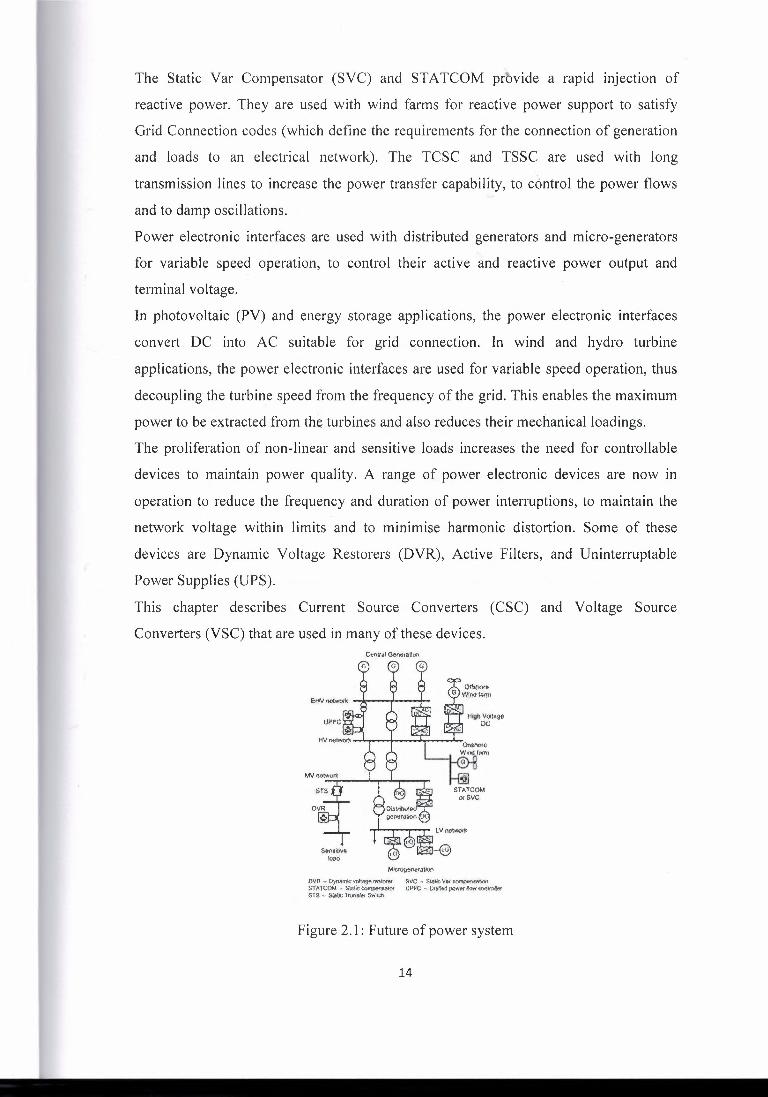
Figure 1.2 shows the DMSC controller building blocks that assess operating conditions

and find the control settings for devices connected to the network. The key functions of

the DMSC are state estimation, bad data detection and the calculation of optimal control

settings.

The DMSC receives a limited number of real-time measurements at set intervals from

the network nodes. The measurements are normally voltage, load injections and power

flow measurements from the primary substation and other secondary substations. These

measurements are used to calculate the network operating conditions. In addition to

these real-time measurements, the DMSC uses load models to forecast load injections at

6

- ·--------------

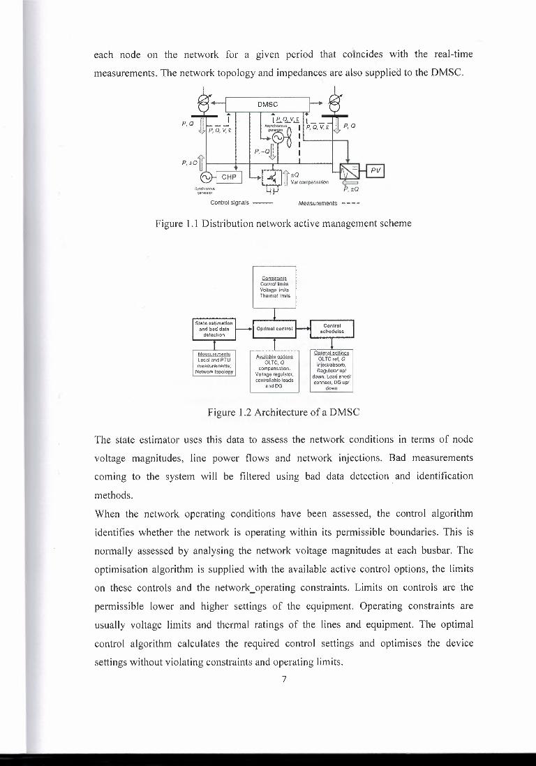
each node on the network for a given period that colncides with the real-time

measurements. The network topology and impedances are also supplied to the DMSC.

4

p Q PL I ' ,B,fp, Q, V,£

DMSC 4

I e...q._vJ; I I ,-------, I

P,±Q

Control signals --- Measurements - - - -

Figure 1.1 Distribution network active management scheme

i&JNlrninJ§. Control limils Voltage limils Thermal limits

51Ate estimation and bad data detection

Control schedules

Optimal s-0ttings OLTC rel, 0 inioct'ebsorb, Regulator up/

down. Load shed/ connect, DG up/

down

Measurements Local and RTU measurements: Network topology -----

fill!ilQble2pJiQllii OLTC, Q

compensation, Voltage regulator, conlrollab!o loads

and OG

Figure 1.2 Architecture of a DMSC

The state estimator uses this data to assess the network conditions in terms of node

voltage magnitudes, line power flows and network injections. Bad measurements

coming to the system will be filtered using bad data detection . and identification

methods.

When the network operating conditions have been assessed, the control algorithm

identifies whether the network is operating within its permissible boundaries. This is

normally assessed by analysing the network voltage magnitudes at each busbar. The

optimisation algorithm is supplied with the available active control options, the limits

on these controls and the network_operating constraints. Limits on controls are the

permissible lower and higher settings of the equipment. Operating constraints are

usually voltage limits and thermal ratings of the lines and equipment. The optimal

control algorithm calculates the required control settings and optimises the device

settings without violating constraints and operating limits.

7

--~--

The solution from the control algorithm is the optimal contrbl schedules that are sent to

the devices connected to the network. Such control actions can be single or multiple

control actions that would alter the set point of any of the devices by doing any of the

following:

• alter the reference of an On-Load Tap Changer (OLTC) transformer/voltage

regulator relay;

• request the Automatic Voltage Regulator (A VR) or the governor of a

synchronous generator to alter the reactive/active power of the machine;

• send signals to a wind farm Supervisory Control and Data Acquisition (SCADA)

system to decrease the wind farm output power;

• connect controllable loads on the network;

• increase or decrease the settings of any reactive power compensation devices;

• Reconfigure the network by opening and closing circuit open points.

1.4.2. Virtual power plant

Distributed energy resources (DER) such as micro-generation, distributed generation,

electric vehicles and energy storage devices are becoming more numerous due to the

many initiatives to de-carbonize the power sector. DERs are too small and too

numerous to be treated in a similar way to central generators and are often connected to

the network on a 'connect-and-forget' basis. The concept of a Virtual Power Plant

(VPP) is to aggregate many small generators into blocks that can be controlled by the

system operator and then their energy output is traded.

Through aggregating the DERs into a portfolio, they become visible to the system

operator and can be actively controlled. The aggregated output of the VPP is arranged to

have similar technical and commercial characteristics as a central generation unit.

The VPP concept allows individual DERs to gain access to and visibility in the energy

markets. Furthermore, system operators can benefit from the optimal use of all the

available capacity connected to the network.

The size and technological make-up of a VPP portfolio have a significant effect on the

benefits of aggregation seen by its participants. For example, fluctuation of wind

generation output can lower the value of the energy sold but variation reduces with

increasing geographical distance between the wind farms. If a VPP assembles

generation across a range of technologies, the variation of the aggregated output of

these generators is likely to reduce.

8

1.5. Impacts and demonstrations of smart grid •

1.5.1. Galvin electricity initiative

The Galvin vision is an initiative that began in 2005 to define and achieve a 'perfect

power system'. The perfect power system is defined as:

"The perfect power system will ensure absolute and universal availability and energy in

the quantity and quality necessary to meet every consumer's needs."

The philosophy of a perfect power system differs from the way power systems

traditionally have been designed and constructed which assumes a given probability of

failure to supply customers, measured by a reliability metric, such as Loss of Load

Probability (LOLP). Consideration of LOLP shows that a completely reliable power

system can only be provided by using an infinite amount of plant at infinite cost.

Some of the attributes of the perfect power system are similar to those of the Smart

Grid.

For example, in order to achieve a perfect power system, the power system must meet

the following goals:

• be smart, self-sensing, secure, self-correcting and self-healing;

• sustain the failure of individual components without interrupting the

service;

• be able to focus on regional, specific area needs;

• be able to meet consumer needs at a reasonable cost with minimum resource

utilisation and minimal environmental impact;

• enhance quality of life and improve economic productivity.

The development of the perfect power system is based on integrating devices (smart

loads, local generation and storage devices), then buildings (building management

systems and micro CHP), followed by construction of an integrated distribution system

(shared resources and storage) and finally to set up a fully integrated power system

( energy optimisation, market systems and integrated operation).

1.5.2. IntelliGridsM

EPRI's IntelliGridsM initiative, which is creating a technical foundation for the Smart

Grid, has a vision of a power system that has the following features:

9

• is made up of numerous automated transmission and distribution systems, all

operating in a coordinated, efficient and reliable manner;

• handles emergency conditions with 'self-healing' actions and is responsive to

energy-market and utility business enterprise needs;

• serves millions of customers and has an intelligent communications

infrastructure enabling the timely, secure and adaptable information flow needed

to provide reliable and economic power to the evolving digital economy.

To realise these attributes, an integrated energy and communication systems

architecture should first of all be developed. This will be an open standard-based

architecture and technologies such as data networking, communication over a wide

variety of physical media and embedded computing will be part of it. This architecture

will enable the automated monitoring and control of the power delivery system, increase

the capacity of the power delivery system, and enhance the performance and

connectivity of the end users. In addition to the proposed communication architecture,

the realization of the IntelliGridSM will require enabling technologies such as

automation, distributed energy resources, storage, power electronic controllers, market

tools, and consumer portals. Automation will become widespread in the electrical

generation, consumption and delivery systems. Distributed energy resources and storage

devices may offer potential solutions to relieve the necessity to strengthen the power

delivery system, to facilitate a range of services to consumers and to provide electricity

to customers at lower cost, and with higher security, quality, reliability and availability.

Power electronic-based controllers can direct power along specific corridors, increase

the power transfer capacity of existing assets, help power quality problems and increase

the efficient use of power. Market tools will be developed to facilitate the efficient

planning for expansion of the power delivery system, effectively allocating risks, and

connecting consumers to markets. The consumer portal contains the smart meter that

allows price signals, decisions, communication signals and network intelligent requests

to flow seamlessly through the two-way portal.

1.5.3. Xcel energy's Smart grid

Xcel Energy's vision of a smart grid includes:

"a fully network-connected system that identifies all aspects of the power grid and

communicates its status and the impact of consumption decisions including economic,

10

environmental and reliability impacts) to automated decision-making systems on that

network."

Xcel Energy's Smart Grid implementation involved the development of a number of

quickhit projects. Even though some of these projects were not fully realised, they are

listed below as they illustrate different Smart Grid technologies that could be used to

build intelligence into the power grid:

1. Wind Power Storage: A 1 MW battery energy storage system to demonstrate

long-term emission reductions and help to reduce impacts of wind variability.

2. Neural Networks: A state-of-the-art system that helps reduce coal slagging and

fouling (build-up of hard minerals) of a boiler.

3. Smart Substation: Substation automation with new technologies for remote

monitoring and then developing an analytics engine that processes data for near

real-time decision-making and automated actions.

4. Smart Distribution Assets: A system that detects outages and restores them using

advanced meter technology.

5. Smart Outage Management: Diagnostic software that uses statistics to predict

problems in the power distribution system.

6. Plug-in Hybrid Electric Vehicles: Investigating vehicle-to-grid technology

through field trials.

7. Consumer Web Portal: This portal allows customers to program or pre-set their

own energy use and automatically control their power consumption based on

personal preferences including both energy costs and environmental factors

1.5.4. SCE's smart grid

Southern California Edison (SCE)'s Smart Grid strategy encompasses five strategic

themes namely, renewable and distributed energy resources integration, grid control and

asset optimisation, workforce effectiveness, smart metering, and energy-smart customer

solutions. SCE anticipates that these themes will address a broad set of business

requirements to better position them to meet current and future power delivery

challenges. By 2020, SCE will have 10 million intelligent devices such as smart meters,

energy-smart appliances and customer devices, electric vehicles, DERs, inverters and

storage technologies that are linked to the grid, providing sensing information and

automatically responding to prices/event signals.

11

SCE has initiated a smart meter connection programme where 5 million meters will be

deployed from 2009 to 2012. The main objectives of this programme include adding

value through information, and initiating new customer partnerships. The services and

information they are going to provide include interval billing, tiered rates and rates

based on time of use.

1.6. Overview of the technologies required for the Smart Grid

Power electronics and energy storage: include:

(a). High Voltage DC (HVDC) transmission and back-to-back schemes and

Flexible AC Transmission Systems (FACTS) to enable long distance

transport and integration of renewable energy sources;

(b) different power electronic interfaces and power electronic supporting

devices to provide efficient connection of renewable energy sources and

energy storage devices;

(c) series capacitors, Unified Power Flow Controllers (UPFC) and other FACTS

devices to provide greater control over power flows in the AC grid;

( d) HVDC, FACTS and active filters together with integrated communication

and control to ensure greater system flexibility, supply reliability and

power quality;

( e) power electronic interfaces and integrated communication and control to

support system operations by controlling renewable energy sources,

energy storage and consumer loads;

(f) energy storage to facilitate greater flexibility and reliability of the power

system.

12

•

Chapter 2

Power electronics and renewable energy

2.1. Introduction

The future power system increasingly will include more controllable power electronic

devices to make the best use of existing circuits, maintain flexibility and optimum

operation of the power system, and to facilitate the connection of renewable energy

resources at all voltage levels. Figure 2.1 illustrates a future power system that is rich in

power electronics.

Current Source Converter High Voltage DC (CSC-HVDCl) is presently used for the

connection of asynchronous power systems (for example, 50-60 Hz), for long overhead

line transmission and submarine cable circuits as well as for the connection of

geographically extensive or weak systems. It is anticipated that CSC-HVDC

connections will be increasingly used in future for inter-country and inter-state

connections.

Voltage Source Converter HVDC (VSC-HVDCl) is used for offshore wind farm

connections. Offshore wind farms up to 50-80 km from shore can be connected to the

terrestrial grid using an AC connection. However, the submarine cables generate

significant reactive power limiting the distance over which an AC cable connection can

be used. The decision on whether to use AC or DC depends on the cable route length,

the number of cables required to transmit the wind farm output, acceptable losses and

capital costs.

Flexible AC Transmission Systems (FACTS) are used to increase the power transfer

capability of existing AC lines, to control steady state and dynamic power flow through

an AC circuit, to control reactive power and voltage and to enhance voltage and angle

stability. Shunt-connected power electronic devices using Thyristors, for example,

Static Var Compensators (SVCs) using Thyristor Controlled Reactors or Thyrsistor

Switched Capacitors

are already widely used. Other FACTS devices, given in Table 2.1, have been

demonstrated.

Other than some commercial applications of STATCOMs, TCSCs, and TSSCs, the use

of other FACTS devices (IPFC and UPFC) has yet to become widespread.

13

The Static Var Compensator (SVC) and STATCOM provide a rapid injection of

reactive power. They are used with wind farms for reactive power support to satisfy

Grid Connection codes (which define the requirements for the connection of generation

and loads to an electrical network). The TCSC and TSSC are used with long

transmission lines to increase the power transfer capability, to control the power flows

and to damp oscillations.

Power electronic interfaces are used with distributed generators and micro-generators

for variable speed operation, to control their active and reactive power output and

terminal voltage.

In photovoltaic (PV) and energy storage applications, the power electronic interfaces

convert DC into AC suitable for grid connection. In wind and hydro turbine

applications, the power electronic interfaces are used for variable speed operation, thus

decoupling the turbine speed from the frequency of the grid. This enables the maximum

power to be extracted from the turbines and also reduces their mechanical loadings.

The proliferation of non-linear and sensitive loads increases the need for controllable

devices to maintain power quality. A range of power electronic devices are now in

operation to reduce the frequency and duration of power interruptions, to maintain the

network voltage within limits and to minimise harmonic distortion. Some of these

devices are Dynamic Voltage Restorers (DVR), Active Filters, and Uninterruptable

Power Supplies (UPS).

This chapter describes Current Source Converters (CSC) and Voltage Source

Converters (VSC) that are used in many of these devices.

Microgon~ratlOn.

DVB.:" Oyn,1cmicvolt~e_.~totfl:r SVC· "' Sw.~ V~( compc<fis!lt0ti $TAJ COM ·"' S!ti!lis Co.m~:ulator UPfC ~ ... unifi~ ~ b .wntn,im- _ST$ .., ,$!a:& 'ft'M1slijt Swlleh

Figure 2.1: Future of power system

14

2.2. Current source converters

The rapid development of semiconductor devices and associated control techniques has

allowed a number of applications of switching power converters in the electric power

system.

Two types of power converter, the Current Source Converter (CSC) and the Voltage

Source Converter (VSC) are in use. In a CSC, the DC side current is kept constant with

a small ripple using a large inductor, thus forming a current source on the DC side. The

r direction of power flow through a CSC is determined by the polarity of the DC voltage

while the direction of current flow remains the same. At present, the CSC is used

mainly in high power applications, particularly for HVDC transmission with a capacity

of up to 7000MW for a single link. In a CSC, the power electronic switches (thyristor

valves) are turned on by control circuits but switch off through natural commutation

when the current through them drops to zero. -

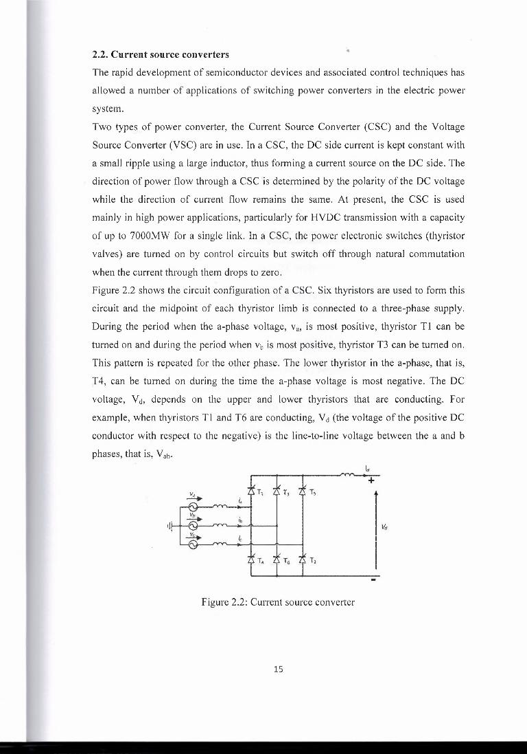
Figure 2.2 shows the circuit configuration of a CSC. Six thyristors are used to form this

circuit and the midpoint of each thyristor limb is connected to a three-phase supply.

During the period when the a-phase voltage, Va, is most positive, thyristor Tl can be

turned on and during the period when vb is most positive, thyristor T3 can be turned on.

This pattern is repeated for the other phase. The lower thyristor in the a-phase, that is,

l4, can be turned on during the time the a-phase voltage is most negative. The DC

voltage, Yct, depends on the upper and lower thyristors that are conducting. For

example, when thyristors Tl and T6 are conducting, V ct (the voltage of the positive DC

conductor with respect to the negative) is the line-to-line voltage between the a and b

phases, that is, Vab· k

~ Y T1 75, T3 ~· r,

+ ' . ·. . . .. ,J~ I

~ '

I \{1

- le.

T.t1 . ti

Figure 2.2: Current source converter

15

Figure 2.3 shows the DC voltage and thyristors that are conducting if they are turned on

without a firing angle delay. The average value of the DC voltage can be obtained by

dividing the shaded area by n/3 (the angle of the shaded area).

OC p0$itive ( +) r~ll vQlt.ig.c with ri/$pOct to ~art.h

OC negative H rail voUa.9\l WI!/\ 1e•rrocl; !o eu.rth Vo!tar,e ac,.oss.oc posmvo (•) aridmigatlve('-) r•il• (Vo)

Figure 2.3: Operation of the CSC without firing angle delay

Since Vd is formed by the line-to-line voltage, its peak value is v'2VLL· So the average

DC voltage is given by:

3 f TI/6 3{2 , TI/6 3{2 Vct = - JzvLL cos(8) de = -VLdsm(8)]_TI/6 = -VLL = 1.35VLL

TT -TI/6 · TT TT

If thyristor Tl is not triggered at the point when Ya becomes more positive than V c or,

in other words, if there is a firing angle delay in Tl, the previous thyristor on the upper

side, that is T5, continues to conduct until Tl is turned on. Figure 2.4 shows the DC

voltage with a firing angle delay of a. Now the shaded area is the integration of same

cosine function, but from -(n/6 - a) to (n/6 + a). Therefore, the average DC voltage is given by..

TI 3 f (6+a) 3{2 . c:!!-a)

Vct = - JzvLLcos(8)d8 = -VLdsm(8)] 6 TI = 1.35VLLcos(cx) rt -Ci-a) TT -(6-a)

16

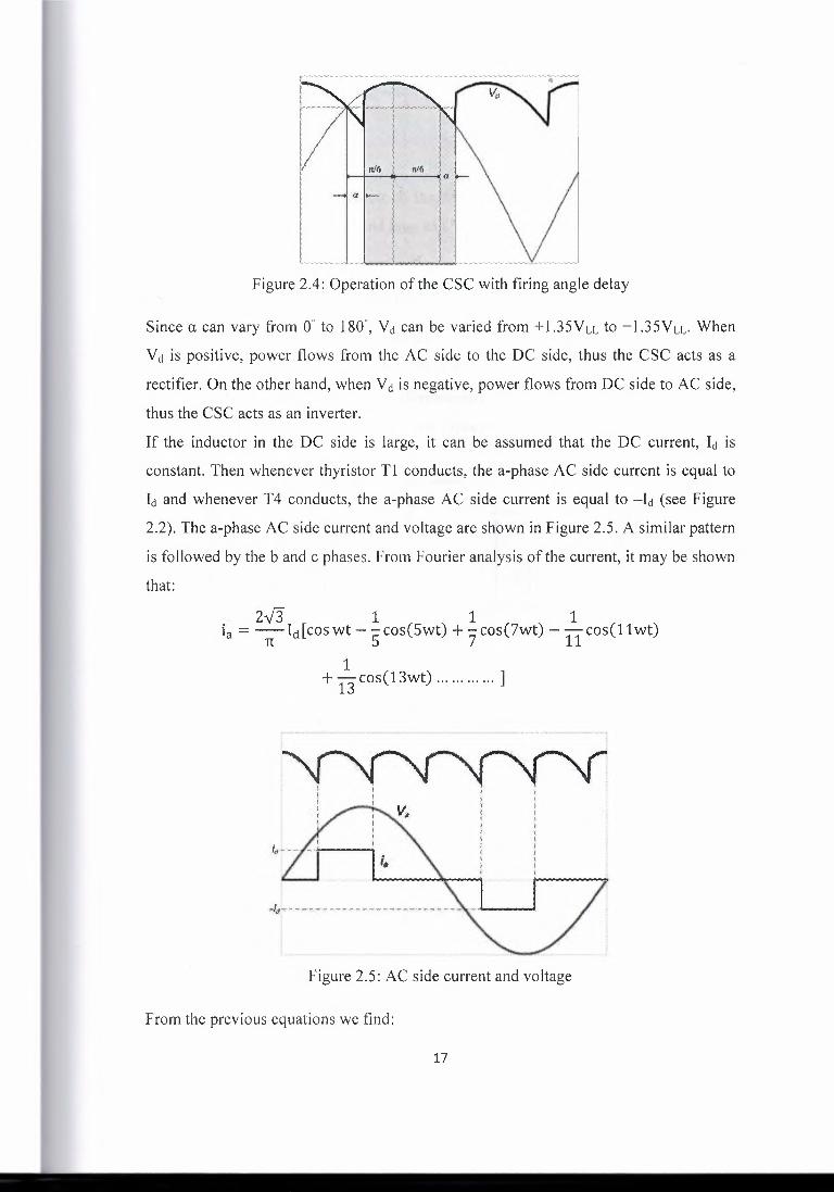
Figure 2.4: Operation of the CSC with firing angle delay

Since a can vary from 0° to 180°, Yct can be varied from +l.35V11 to -l.35V11. When

Vct is positive, power flows from the AC side to the DC side, thus the CSC acts as a

rectifier. On the other hand, when Vct is negative, power flows from DC side to AC side,

thus the CSC acts as an inverter.

If the inductor in the DC side is large, it can be assumed that the DC current, lct is

constant. Then whenever thyristor Tl conducts, the a-phase AC side current is equal to

lct and whenever T4 conducts, the a-phase AC side current is equal to -lct (see Figure

2.2). The a-phase AC side current and voltage are shown in Figure 2.5. A similar pattern

is followed by the band c phases. From Fourier analysis of the current, it may be shown

that:

2'13 1 1 1 ia = ~Ict[coswt-5cos(Swt) + 7cos(7wt) -11cos(11wt)

1 + 13

cos(13wt) ]

Figure 2.5: AC side current and voltage

From the previous equations we find:

17

2y3 The peak value of the fundamental= -Id TI

16 Therefore therms value= - Id TI

Ignoring losses and equating power on the AC and DC sides: 3VRMsIRMs cos cp = Yctlct,

Substituting for VRMs = VLJ-'13 and IRMs and Yct from previous Equations, the following

equations can be obtained:

Vu- -v6 3-v2 3 x r::; x -Id cos(0) = -Vucos(a) x Id

v3 TI TI

cos(0) = cos(a) 0=a

As the angle a changes, the phase displacement between the AC side voltage and

current of the CSC also changes. From last Equation, the power factor angle is equal to

a.

Figure 2.6: The commutation process

·•JaiL. 1t

l .15Vuc;l$'( r1L\ _

Figure 2. 7: Equivalent circuit in rectifier mode

In the preceding section it is assumed that the commutation process is instantaneous. In

other words, one thyristor stops conducting suddenly and transfers the current to the

next thyristor immediately. However, this is not true as the system inductance does not

allow the current through a thyristor to extinguish suddenly. Figure 2.6 shows

commutation from T3 to T5 (that is, T3 will stop conducting and T5 will start

18

conducting at this instance). As shown in Figure 2.6, V d is nd longer V baas there will be

a circulating current between T3 and T5.

This circulating current reduces the average value of the DC side voltage. It can be

shown that Yct = l.35VLL cos a - (3coL/n )Ict. From this equation, a DC equivalent

circuit of the rectifier, which is a DC source of magnitude 1.35V LL cos a and a series

resistance (not a physical resistor but an equivalent resistance to represent the

commutation process) of (3coL)/n (as shown in Figure 2.7), can be derived.

2.3. Voltages source converters

A converter where the DC side voltage is maintained as constant using a large capacitor

is called a VSC. The VSC is widely used for low and medium power applications such

as grid connection of micro-generation, renewable energy sources, and energy storage.

However, the VSC is also used at power levels up to 1000 MW for HVDC transmission.

The semiconductor devices that are used in YSC are rapidly increasing in size and

reducing in cost. Therefore, it is anticipated that YSC technology will dominate high

power DC applications in future. The VSC offers advantages such as freedom to operate

with any combination of active and reactive power, the ability to operate in a weak grid

and even black-start, fast acting control, the possibility of using voltage polarised cables

and generating good sinusoidal wave-shapes. Hence it is anticipated that it will be the

choice of future converters.

A YSC employs controllable switches where current can be controlled in the forward

direction and an anti-parallel diode is provided for current flow in the reverse direction.

The current in the forward direction can be switched on and off. Commonly used

semiconductor switches include Metal Oxide Semiconductor Field Effect Transistor

(MOSFET), Insulated Gate Bipolar Transistor (IGBT), Gate Turn-off Thyristor (GTO),

and Insulated Gate Commutated Thyristor (IGCT). The current and voltage ratings of

MOSFETs are limited and therefore they are only used for low power applications.

IGBTs have been used in both low and medium power applications. As their current and

voltage ratings increase, it is anticipated that IGBT switches will be used in high power

applications (already a few HVDC projects of up to 500MWare employing them). The

IGCT is evolving as a device having lower on-state losses (compared to an IGBT) and

faster switching times ( compared to a OTO) and is used in some high power

applications.

19

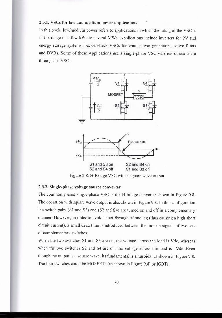
2.3.1. VSCs for low and medium power applications

In this book, low/medium power refers to applications in which the rating of the VSC is

in the range of a few kWs to several MWs. Applications include inverters for PY and

energy storage systems, back-to-back VSCs for wind power generators, active filters

and DVRs. Some of these Applications use a single-phase VSC whereas others use a

three-phase VSC.

t V•ct.¢' '~.

2

V

Fimtlo;me:1jtal

)I; ,t< :;,r•

"' /.

.S1 ~tldSS on S2and:s4 Off.

S2andS4on si. and S3 off

Figure 2.8: H-Bridge VSC with a square wave output

2.3.2. Single-phase voltage source converter

The commonly used single-phase VSC is the H-bridge converter shown in Figure 9.8.

The operation with square wave output is also shown in Figure 9.8. In this configuration

the switch pairs (SI and S3) and (S2 and S4) are turned on and off in a complementary

manner. However, in order to avoid shoot-through of one leg (thus causing a high short

circuit current), a small dead time is introduced between the turn-on signals of two sets

of complementary switches.

When the two switches S 1 and S3 are on, the voltage across the load is V de, whereas

when the two switches S2 and S4 are on, the voltage across the load is -Vdc. Even

though the output is a square wave, its fundamental is sinusoidal as shown in Figure 9.8.

The four switches could be MOSFETs (as shown in Figure 9.8) or IGBTs.

20

Due to the harmonics produced by the square wave voltage output,

switching strategy is only used with off-grid low

applications a sine-triangular Pulse Width Modulation (FWM) technique is used to

control the tum-on and tum-off times of the four switches. The switching instances are

determined by comparing a sinusoidal modulating signal with a triangular carrier signal

(see Figure 9.9). When the magnitude of the carrier is higher than the modulating signal,

S2 and S4 are turned on. On the other hand, when

the magnitude of the carrier is lower than the modulating signal, S 1 and S3 are turned

on.

Modulating sfgnal Frequency (m Amplitude A,,,

C;1rrje( sign.ii Freq(Jeooy f. AmpUlude A.

PWM waveform F.undamenlal

Figure 2.9: PWM output voltage

The PWM output voltage has a fundamental component and a series of harmonics.

Harmonic frequencies depend on the frequency modulation index, mf, which is defined

as the ratio between fc (frequency of the Carrier signal) and fm (frequency of the

Modulating signal). The harmonics are at frequencies (pm, + q) fin, where p = 1, 2, 3 .. . . etc .. When p is odd then q is zero or even, that is if p = 3, harmonics will occur at

3mf fin, (pm, +2)fm, (pm- +4 jfm and so on. When p is even then q is odd, that is if p =

2, harmonics will occur at (pmf+ l jfrn, (pmr+ 3)fm and so on.

As each switch is turned on and off many times in a cycle, a VSC switched by a PWM

technique produces more switching losses than a VSC that produces square waves.

However, square wave VSC operation is less attractive due to the low order harmonics

it generates and the filtering needed to control these harmonics.

Figure 2.10 shows the PWM pattern shown in Figure 2.9 for two different amplitude

modulation indexes. As can be seen from Figure 2.10, the average of the PWM pattern

21

------~- ------------- ---------- ---------

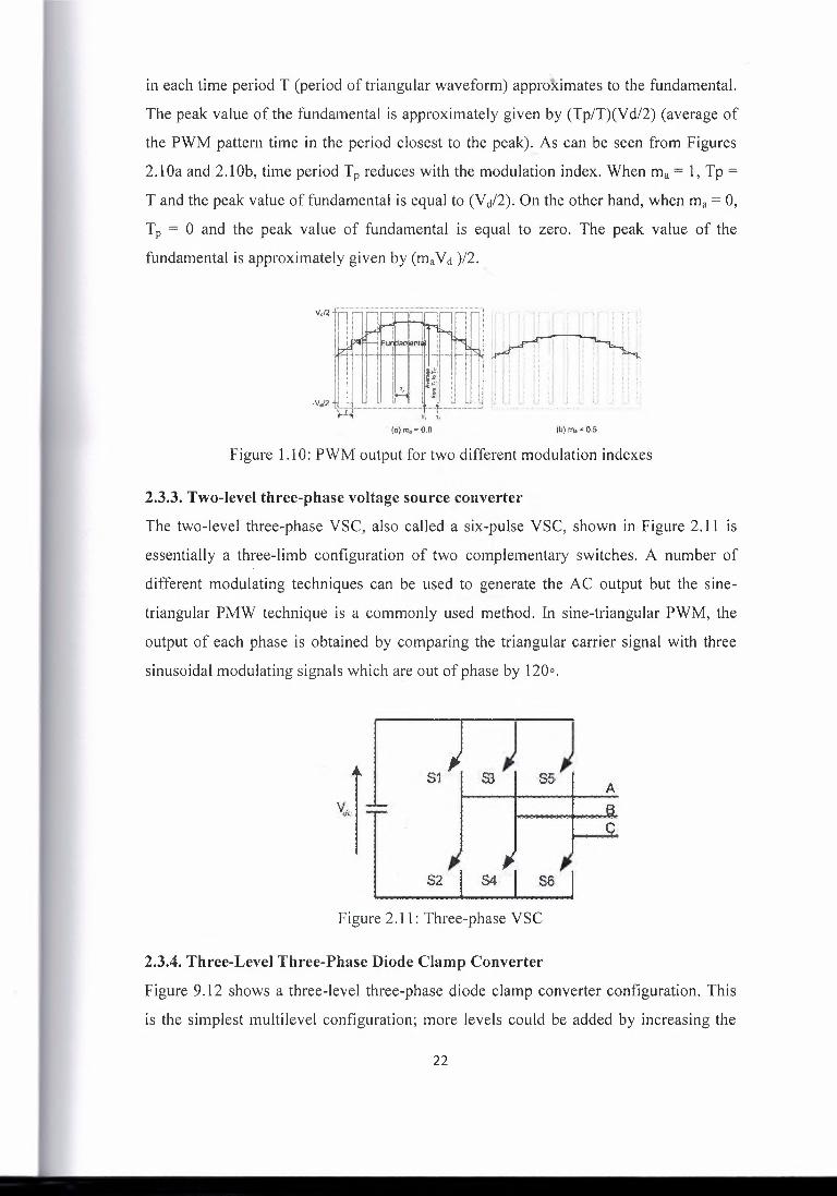
in each time period T (period of triangular waveform) approximates to the fundamental.

The peak value of the fundamental is approximately given by (Tp/T)(V d/2) ( average of

the PWM pattern time in the period closest to the peak)., As can be seen from Figures

2.1 Oa and 2.1 Ob, time period T P reduces with the modulation index. When ma = 1, Tp =

T and the peak value of fundamental is equal to (V ctl2). On the other hand, when ma= 0,

T, = 0 and the peak value of fundamental is equal to zero. The peak value of the

fundamental is approximately given by (rn.V, )/2.

Figure 1.10: PWM output for two different modulation indexes

(B)m,,=.0,8 (b) rt>,• 0.5

2.3.3. Two-level three-phase voltage source converter

The two-level three-phase VSC, also called a six-pulse VSC, shown in Figure 2.11 ts

essentially a three-limb configuration of two complementary switches. A number of

different modulating techniques can be used to generate the AC output but the sine­

triangular PMW technique is a commonly used method. In sine-triangular PWM, the

output of each phase is obtained by comparing the triangular carrier signal with three

sinusoidal modulating signals which are out of phase by 120°.

Figure 2.11: Three-phase VSC

2.3.4. Three-Level Three-Phase Diode Clamp Converter

Figure 9.12 shows a three-level three-phase diode clamp converter configuration. This

is the simplest multilevel configuration; more levels could be added by increasing the

22

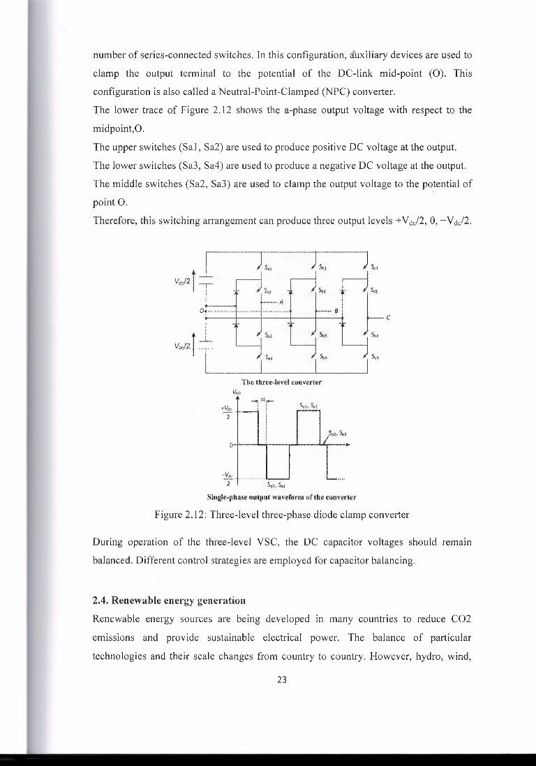
number of series-connected switches. In this configuration, auxiliary devices are used to

clamp the output terminal to the potential of the DC-link mid-point (0). This

configuration is also called a Neutral-Point-Clamped (NPC) converter.

The lower trace of Figure 2.12 shows the a-phase output voltage with respect to the

midpoint,O.

The upper switches (Sal, Sa2) are used to produce positive DC voltage at the output.

The lower switches (Sa3, Sa4) are used to produce a negative DC voltage at the output.

The middle switches (Sa2, Sa3) are used to clamp the output voltage to the potential of

point 0.

Therefore, this switching arrangement can produce three output levels +Yctc/2, 0, -Vctcf2.

. . I V~J2l

. Jf.f ·. · S ...•.. ,.·., .2 .

C

... ,··s..

-V"' . 2 ! · S,i;.S,,

Single-phase output waveform of Ute converter

Figure 2.12: Three-level three-phase diode clamp converter

During operation of the three-level VSC, the DC capacitor voltages should remam

balanced. Different control strategies are employed for capacitor balancing.

2.4. Renewable energy generation

Renewable energy sources are being developed in many countries to reduce CO2

emissions and provide sustainable electrical power. The balance of particular

technologies and their scale changes from country to country. However, hydro, wind,

23

biomass (solid biomass, bioliquids and biogas), tidal stream: and photovoltaic (PV) are

common choices.

Variable speed turbines are used for wind, small hydro and tidal power generation.

These generally use AC-DC-AC power conversion where the turbine is arranged to

rotate at optimum speed to extract the maximum power from the fluid flow or minimize

mechanical loads on the turbine. The variable frequency power output from the

generator is first converted to DC. A second converter is used to convert DC into 50/60

Hz AC.

The output of a PV system is DC and therefore a DC-AC converter is essential for grid

connection. Biomass technologies use a steam or gas turbine and a conventional

generator.

Reciprocating engines may be fuelled by biogas. They generally use a synchronous

generator connected to the grid directly and are not considered in this chapter.

The power electronic interface between a renewable energy source and the grid can be

used to control reactive power output and hence the network voltage as well as

curtailing real power output, and so enable the generator to respond to the requirements

of the grid.

2.4.1. Photovoltaic systems

Photovoltaic (PV) systems which convert solar power directly into electricity are being

installed in increasing numbers in many countries, for example, Germany, Spain, the

USA and Japan. Feed-in-tariffs, which provide guaranteed payment per unit of

electricity (p/kWh) for renewable electricity generation, have been particularly

important in stimulating the uptake of PV.

Figure 2.13 shows the main elements of a grid-connected domestic PV system. It

typically consists of:

(I) a DC-DC converter for Maximum Power Point Tracking (MPPT) and to increase

the voltage;

(2) a single

filter

phase

and sometimes

DC-AC inverter;

a transformer; and (3) an output

( 4) a contra lier.

24

DC-DC converter

Single ph.ise inverter

Flltetand grid

lnlerface

Controller for MPPT, PWM, Reactive. power comrot,

1/0ltage control. ..

Interface to Homo Area Network or Smart meter

Figure 2.13: Block diagram of a domestic PV system

A

500Wlm2

I sopw1mi I

o1YM•--ibc.~ -c, ,,,ch J. (1 20 40

Voltage (V).

00 20 40 Voltage(V)

Figure 2.14: Typical current/voltage and power/voltage characteristics of a PV module

for irradiance

The PV module contains a number of photovoltaic cells connected in series and in

parallel. Figure 2.14 shows the current versus voltage and the power versus voltage

characteristics of a PV module. The maximum power output of the module is obtained

near the knee of its voltage/current characteristic.

Different configurations of DC-DC converters are used, for example, boost, push-pull,

full bridge, and flyback converter. The DC voltage on the inverter side of the DC-DC

converter is normally maintained to be constant by the inverter control. The MPPT

algorithm is used to find continually a PV array DC voltage which extracts the most

power from the PV array while the cell temperatures and operating conditions of the

module change.

25

As it is easy to implement in a digital controller, the most widely used MPPT algorithm

is 'perturb and observe' sometime known as 'hill climbing'. In this method, the terminal

voltage of the PV array is perturbed in one direction and if the power from the PV array

increases, then the operating voltage is further perturbed in the same direction.

Otherwise if the power from the PV array decreases, then the operating voltage is

perturbed in the reverse direction. Another technique more easily implemented with

analogue electronics is incremental conductance.

This is based on the fact that at maximum power point, (di/dv) + (i/v) of the PV array is zero (derived from dP/dv = 0). This equation suggests that the voltage corresponding to

the maximum power can be found by measuring the incremental conductance (di/dv)

and instantaneous conductance (i/v).

The DC voltage obtained from the DC-DC converter is inverted to 50/60 Hz AC. A

voltage source inverter is widely used. As discussed, this normally uses a pulse width

modulation switching technique to minimize harmonic distortion. Finally, a filter is

placed at the output to minimise harmonics fed into the power system. In some designs

a transformer is also employed at the output of the inverter to ensure no DC is injected

into the grid.

2.4.2. Wind, hydro and tidal energy systems

Wind, hydro and tidal generation systems all involve converting the potential and/or

kinetic energy in water or air into electrical energy. In recent years there has been a

dramatic increase in power generation from the wind with the capacity of wind turbines

that have been installed across the globe now approaching 200 GW. Hydropower is a

mature technology with units varying in size from a few kW to hundreds of MW. Tidal

stream generation is a more recent innovation and the subject of considerable research

and development effort.

Wind farms are now being developed both onshore and offshore. Placing a wind turbine

in the sea is more challenging and expensive but offshore wind farms enjoy a stronger

and more consistent wind resource and reduced environmental impact. The majority of

generators used in offshore wind turbines are variable speed. Some years ago, fixed

speed wind turbines were common onshore but the majority of new onshore

installations also use variable speed wind turbines.

In developed countries the economically attractive sites for large hydropower plants

have now almost all been exploited but there are still opportunities for the development

26

of small and micro hydropower plants. The efficiency of these smaller units across a

wide range of water flows can be improved by using a variable speed generator with a

power electronic interface.

Different turbine designs are available for tidal stream technologies [5]. Some stand on

the seabed and are shrouded and some are floating. They can be categorised into:

1. Horizontal axis turbines: The architecture of these turbines is similar to that of wind

turbines.

2. Vertical axis turbines: Vertical axis turbines do not require orientation into the flow

but do suffer from large cyclic torques.

3. Oscillating hydrofoil devices: These have hydrofoils which move back and forth in a

plane normal to the tidal stream.

4. Ducted devices: The tidal flow is directed through a duct and a smaller diameter

turbine is situated inside the duct.

Turbine

.Qout>ly•F'ed !nduqtiori · Generator

aaclNo,Bd; Vtl0$ :i;ortri~t~tt

.to Ihm ro.tor

Geared Full Power ConvcH1.er

B.!ci\•lo-Ballk \/SC# coooccloo

to Uio ,i.la!m

Gearless Full Power . . converter

Mµlitsp()1e ~imMenl magnel

· ayoci1rooou1; 9e!Ji<!r1d.or

Figure 2.15: Different variable speed generator configurations

27

Chapter 3

Control systems using microcontroller and MATLAB

3.1. What is a Microcontroller?

A micro-controller is a small computer on a single integrated circuit containing a

processor core, memory, and programmable input/output peripherals.

The important part for us is that a micro-controller contains the processor (which all

computers have) and memory, and some input/output pins that you can control. (often

called GPIO - General Purpose Input Output Pins).

Figure 3.1: Arduino Board

For this book, we will be using the Arduino Uno board. This combines a micro­

controller along with all of the extras to make it easy for you to build and debug your projects.

Arduino is an open-source microcontroller board, with an associated development

environment. The schematics and the software are released under the Creative

Commons License.

Manufacturing and distributing an official Arduino product is subject to a few

restrictions (basically the authors need to be contacted) to make sure that:

• Things work properly.

• The product fits into the overall project.

• It is manufactured under reasonably fair labor conditions.

3.1.1. Specification (Arduino)

• A Tmega328 microcontroller

• 16 MHz, 32 KB FLASH, 2KB SRAM, lK EEPROM 28

• 19 DIO pins (6 can be 8-bits 500Hz PWM outputs) •

• 6 analog inputs (10 bits over 0-5V range, 15kSPS)

• 5V operating voltage, 40 mA DC Current per IO Pin

• I2C (TWI) fully supported and SPI partially supported

• USB connection (FTDI chip converts USB to Serial)

• FTDI Drivers provide a virtual com port to the OS

• Power jack and optional 9V power supplier

3.1.2. Shields

• Shields are boards to be mounted on top of the Arduino

• They extend its functionality to control different devices, acquire data, and so C'

on ...

• Examples:

• Motor/Stepper/Servo Shields (Motor Control)

• Multichannel Analog and Digital IO Shields

• Prototyping Shields

• Ethernet and Wireless communication Shields

• Wave Shields (Audio)

• GPS and Logging Accelerometer Shields

• Relay Control Shields

We will be using a test board in our project; this is a relatively easy way to make

circuits quickly. Test boards are made for doing quick experiments. They are not known

for keeping circuits together for a long time. When you are ready to make a project that

you want to stay around for a while, you should consider an alternative method such as

wire-wrapping or soldering or even making a printed circuit board (PCB).

The first thing you should notice about the test board is all of the holes. These are

broken up into 2 sets of columns and a set of rows (the rows are divided in the middle).

The columns are named a, b, c, d, e, f, g, h, i, and j (from left to right). The rows are

numbered 1 - 30. (from top to bottom). The columns on the edges do not have letters or

numbers. The columns on the edges are connected from top to bottom inside of the test

board to make it easy to supply power and ground. (You can think of ground as the

negative side of a battery and the power as the positive side.)

For our project power will be +5 volts. Inside of the test board, the holes in each row are

connected up to the break in the middle of the board.

29

For Example: al, bl, cl, dl, el all have a wire inside of the'test board to connect them.

Then fl, g 1, h 1, i I, and j 1 are all connected. but a 1 is not connected to fl. This may

sound confusing now, but it will quickly come to make sense as we wire up circuits.

Figure 3.2: Test board

3.1.3. What is Arduino good for? ' • Projects requiring Analog and Digital IO

• Mechatronics Projects using Servo, DC or Stepper Motors

• Projects with volume/size and/or budget constraints

• Projects requiring some amount of flexibility and adaptability (i.e. changing

code and functions on the fly)

• Basically any Mechatronics project requiring sensing and acting, provided that

computational requirements are not too high (e.g. can't do image processing

with it)

• Ideal for undergraduate/graduate Mechatronics Labs and Projects

• There is a very large community of people using it for all kind of projects, and a

very lively forum where it is possible to get timely support

3.2. Install the software

If you have access to the internet, there are step-by-step directions and the software

available at: here. Otherwise, the USB stick in your kit has the software under the

Software

Directory. There are two directories under that. One is "Windows" and the

other is "Mac OS X". If you are installing onto Linux, you will need to follow the

directions at: here

3.2.1. Windows Installation

1. Plug in your board via USB and wait for Windows to begin its driver installation

process. After a few moments, the process will fail. (This is not unexpected.)

2. Click on the Start Menu, and open up the Control Panel. 30

3. While in the Control Panel, navigate to System and Security. Next, click on System.

Once the System window is up, open the Device Manager.

4. Look under Ports (COM & LPT). You should see an open port named "Arduino

UNO (COMxx)".

5. Right click on the "Arduino UNO (COMxx)" port and choose the "Update Driver

Software" option.

6. Next, choose the "Browse my computer for Driver software" option.

7. Finally, navigate to and select theUno's driver file, named "ArduinoUNO.inf',

located in the "Drivers" folder of the Arduino Software download (not the "FTDI

USB Drivers" sub-directory).

8. Windows will finish up the driver installation from there.

9. Double-click the Arduino application.

10. Open the LED blink example sketch: File> Examples> I.Basics> Blink.

11. Select Arduino Uno under the Tools> Board menu.

12. Select your serial port (if you don't know which one, disconnect the UNO and the

entry that disappears is the right one.)

13. Click the Upload button.

14. After the message "Done uploading" appears, you should see the "L" LED blinking

once a second. (The "L" LED is on the Arduino directly behind the USB port.)

3.2.2. The integrated Development Environment (IDE)

You use the Arduino IDE on your computer (Figure 3 .3) to create, open, and change

sketches. Sketches define what the board will do. You can either use the buttons along

the top of the IDE or the menu items.

In our project we will use Arduino IDE only one time to load the main program to the

board that make programming Arduino micro-controller from MA TLAB/Simulink

possible.

31

Lsave Open

New Upload

Verify

Figure 3.3: Arduino IDE

Parts of the IDE: (from left to right, top to bottom)

• Compile -Before your program"code" can be sent to the board, it needs to be

converted into instructions that the board understands. This process is called

compiling.

• Stop-This stops the compilation process. (I have never used this button and you

probably won't have a need to either.)

• Create new Sketch-This opens a new window to create a new sketch.

• Open Existing Sketch - This loads a sketch from a file on your computer.

• Save Sketch-This saves the changes to the sketch you are working on.

• Upload to Board - This compiles and then transmits over the USB cable to your

board.

• Serial Monitor.

• Tab Button - This lets you create multiple files in your sketch. This is for more

advanced programming than we will do in this class.

• Sketch Editor.

• Text Console - This shows you what the IDE is currently doing and is also

where error messages display if you make a mistake in typing your program.

(often called a syntax error).

32

• Line Number -This shows you what line number your cursor is on. It is useful

since the compiler gives error messages with a line number.

3.3. Arduino board and MATLAB

3.3.1. Challenges with Mechatronics projects

3.3.1.1. Sensing & Data Acquisition

• Distance/Range, Position/Orientation, Force/Pressure, Touch, Orientation,

Motion/Speed, Environment, Optical, Chemical, Flow, Voltage/Current, sensor

selection is largely application related but also related to:

• Data acquisition system (Analog and Digital input)

• Number of sensors

• Ranges

• AID conversion issues as Resolution and Sampling Rate

• Signal Conditioning

• Delay/Bandwidth

3.3.1.2. Processing & Programming Platform

• External Microcontroller/Microprocessor Board

• Development-Prototyping Environment

• Low-Level Programming Language, Compiler/Assembler

• Connection to computer (or LCD) for visualization

• DAQ typically already there

• Stand Alone Issues, power requirements

• Computer

• Connection to DAQ (USB, PCI, Serial, Wireless)

• Programming-Analysis Environment

• OS I Drivers (Real Time?)

• Embedded I Small Form Factor Computer

3.3.1.3. Acting (Digital & Analog Outputs, PWM)

• Relays

• Motors

• DC/Steppers/Servos.

33

• Signal Amplification

• ' Power Suppliers, Batteries

• Forward/Reverse, H-Bridges

• Displays

•

3.3.1.4. Lots of (interrelated) choices

Driving factors:

• Cost

• Easy to use

• Flexibility

• Non trivial process even for simple projects.

• Some challenges are inherent to the multidisciplinary nature of the field and it's

good for students to struggle with them ( e.g. sensors, actuators, power, design)

• Some are not ( e.g. debugging C code, drivers issues, hardware limitations,

unreadable manuals, high costs)

3.3.2. MathWorks Solution

• Arduino IO Package:

Used to perform analog and digital input and output as well as motor control from

the MATLAB command line

• Arduino Target:

Used to compile and download Simulink® code directly to the Arduino board

Figure 3.4: Arduino 10 - Concept

34

3.3.2.1. Using MATLAB vs. IDE Environment

• MATLAB is more interactive, results from Digital/ Analog 1/0 instructions can

•

be seen immediately without needing to program - compile - upload - execute

each time.

It is a good idea even just for algorithm prototyping

• MATLAB code is generally more compact and easier to understand than C

(higher-abstraction data types, vectorization, no need for

initialization/allocation, less lines of code) which means:

a) MATLAB scales better with project complexity

b) People get the job done faster in MATLAB

• For wider-breadth projects (that might include data analysis, signal processing,

calculations, simulation, statistics, control design ... ) MATLAB is better suited

• Engineering Departments typically need to introduce MATLAB during the first

years, so this package will allow professors to keep the same environment and

students to practice more MATLAB

• People might already be more familiar with MATLAB than with C, both in

industry and university

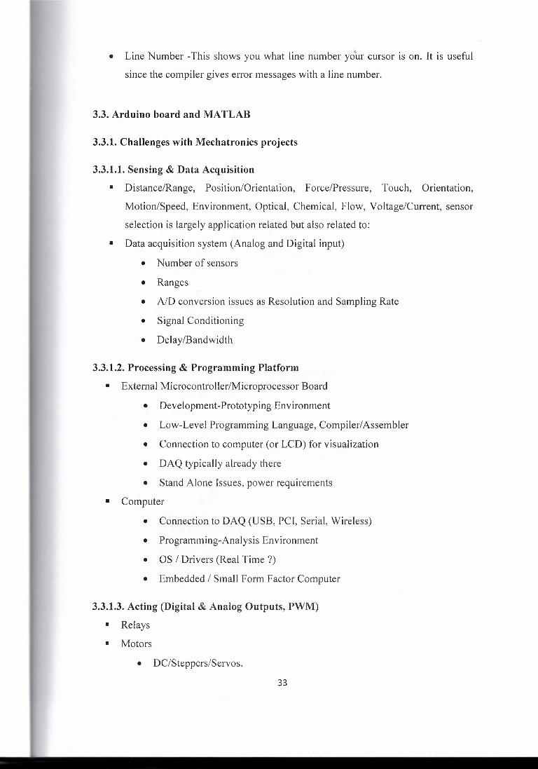
3.3.2.2. Analog and Digital IO

Plug board Connect

USE

Assign Pin Mode Digital Input Digital Output Analog Input Analog Output

Disconnect Unplug

Figure 3.5: Connect diagram

• Connect:

Use the command a=arduino('port'), with the right COM port as a string input

argument, to connect MATLAB with the board and create an arduino object in

the workspace:

35

>> a=arduino('COM5');

• Assign Pin Mode (input/output)

Use the command a.pinMode(pin,str) to get or set the mode of a specified pin:

•

• Examples:

>> a.pinMode(l 1,'output')

>> a.pinMode(l O,'input')

>> val=a.pinMode(lO)

>> a.pinMode(5)

>> a.pinMode;

• Digital Read (digital input)

Use the command a.digitalRead(pin) to read the digital status of a pin:

• Examples:

>> val=a.digita1Read(4)

This returns the value (0 or 1) of the digital pin number

T ... 11'. :·,:~ .. ,,.~ .... .,

a 1Ni:i<.""'"'°"J~ r l, •• ~ i,, , .. ,_9,,..,-,-<,., r com11·". ood .

executed while M-" = nunon is re_!easod

HATIAfl ,. Comruann "cJt- Comrnand Wmdow ,,._,, ~.<:h.p:1: .. <"1.~r>r,.i<:1 di 4:t exeo...1tedwh1!e

button rs p1essfltl I "'a~ =

Figure 3.6: Digital Read example

• Digital Write (digital output)

Use the command a.digitalWrite(pin,val)with the pin as first argument and the

value (0 or 1) as second argument:

• Examples:

a.digita1Write(l3,l); % sets pin #13 high

a.digita1Write(13,0); % sets pin #13 low

36

----·------

f '"""''·~,·~ J, MATLAB ·t L:ti- Command

I Windo)v

l '::' (lH;-¥.c\i:,!

PWM..,.f41 PWM14(S)1

Pwr1_,m, 'ciJOOI

Figure 3.7: Digital Write example

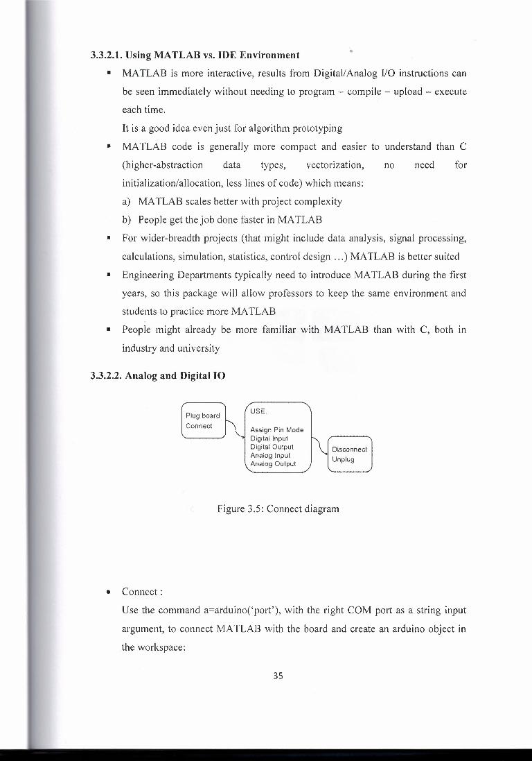
• Analog Read (analog input)

Use the command val=a.analogRead(pin) with the pin as an integer argument:

• Example:

val=a.analogRead(O); % reads analog pin # 0

• The returned argument ranges from O to 1023.

• Note that 6 analog input pins (0 to 5) coincide with the digital pins 14 to

19 and are located on the bottom right corner of the board

MATLAB ·\. Command Window'\.

'"" )<

Figure 3.7: Analog read example

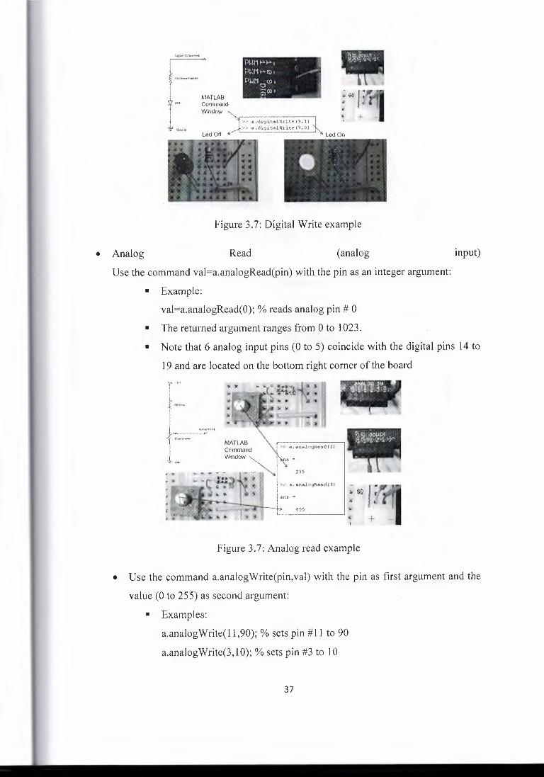
• Use the command a.analogWrite(pin,val) with the pin as first argument and the

value (0 to 255) as second argument:

• Examples:

a.analogWrite(l 1,90); % sets pin #11 to 90

a.analogWrite(3,10); % sets pin #3 to 10

37

.. ~.::~ ,, l MATLAB

I·.u.o Command Window ,.

-;·.:,,,i,:;w,ec

a. an~l,:igWri t e ('9·1 10)

Figure 3.8: Analog write example

• Disconnect

Use the command delete(a) to disconnect the MATLAB session from the

Arduino board: "

>> delete(a);

This renders the serial port available for other sessions or the IDE environment.

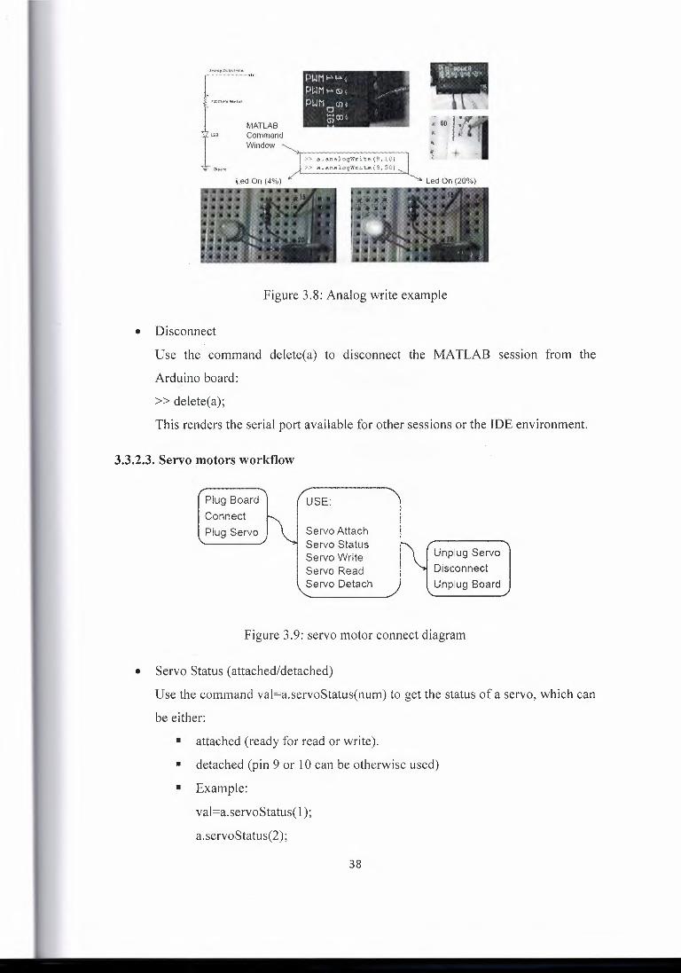
3.3.2.3. Servo motors workflow

Plug Board Connect Plug Servo

USE:

Servo Attach Servo Status Servo Write Servo Read Servo Detach

Unplug Servo Disconnect Unplug Board

Figure 3.9: servo motor connect diagram

• Servo Status (attached/detached)

Use the command val=a.servoStatus(num) to get the status of a servo, which can

be either:

• attached (ready for read or write).

• detached (pin 9 or 10 can be otherwise used)

• Example:

val=a.servoStatus(l);

a.servoStatus(2);

38

a.servoStatus;

• Servo attach

Use the command a.servoAttach(num) to attach a servo to the corresponding

pwm pin (servo #1 uses pin #10, servo #2 uses pin #9).

• Example:

a.servoAttach(l); % attach servo #1

a.servoAttach(2); % attach servo #2

• Servo Read

Use the command val=a.servoRead(num) to read the angle from a servo. The

argument is the number of the servo.

The returned value is the angle in degrees, typically from Oto 180.

• Example:

val=a.servoRead(l ); % read angle servo # 1

val=a.servoRead(2); % read angle servo #2

• Servo Write

Use the command a.servo Write(num,val) to rotate a servo of a given angle.

The first argument is the number of the servo, the second is the angle.

• Example:

a.servoWrite(l,45); % rotates 45° servo #1

• Servo Detach

Use the command a.servoDetach(num) to detach a servo from the corresponding

pwmpm.

• Example:

a.servoDetach(l); % detach servo #1

a.servoDetach(2); % detach servo #2

39

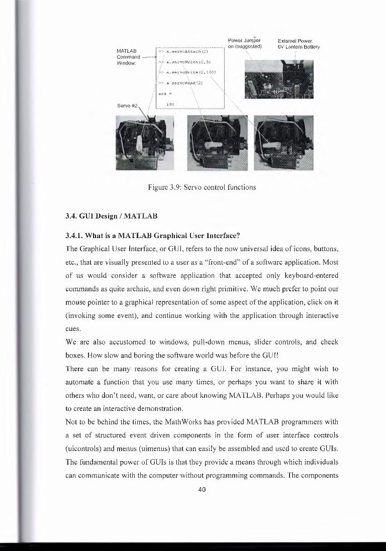
MATLAB Command Window:

• Power Jumper on (suggested)

External Power: 6Vlantern Battery

Servo#2

Figure 3.9: Servo control functions

3.4. GUI Design I MATLAB "'

3.4.1. What is a MATLAB Graphical User Interface?

The Graphical User Interface, or GUI, refers to the now universal idea of icons, buttons,

etc., that are visually presented to a user as a "front-end" of a software application. Most

of us would consider a software application that accepted only keyboard-entered

commands as quite archaic, and even down right primitive. We much prefer to point our

mouse pointer to a graphical representation of some aspect of the application, click on it

(invoking some event), and continue working with the application through interactive

cues.

We are also accustomed to windows, pull-down menus, slider controls, and check

boxes. How slow and boring the software world was before the GUI!

There can be many reasons for creating a GUI. For instance, you might wish to

automate a function that you use many times, or perhaps you want to share it with

others who don't need, want, or care about knowing MATLAB. Perhaps you would like

to create an interactive demonstration.

Not to be behind the times, the Math Works has provided MATLAB programmers with

a set of structured event driven components in the form of user interface controls

(uicontrols) and menus (uimenus) that can easily be assembled and used to create GUis.

The fundamental power of GUis is that they provide a means through which individuals

can communicate with the computer without programming commands. The components

40

have become quite standardized and developed into a user friendly and intuitive set of

tools.

These tools can be used to increase the productivity of a user or to provide a window to

the sophistication and power of a MATLAB application for people with little or no

MATLAB programming experience.

The set of user interface components supplied with MATLAB allows you to design

GUis that match those used in sophisticated software packages. Considering the great

deal of flexibility and usefulness that these objects provide, the programming required

to design a fully functional GUI is amazingly simple. The uicontrols and uimenus can

be combined with other graphics objects to create informative, intuitive, and

aesthetically pleasing GUis. This chapter is designed to make you aware of all the user

interface capabilities and to show you how to program fully functional GUis that meet

your needs. In addition to showing how to create and program uicontrol and uimenu

objects, this chapter will also attempt to broaden your programming horizons by

showing how you can use the other graphics objects previously discussed to design your

own interface components.

The first approach is a low-level, bottom-up approach where we use our skills with

handle graphics to write M-files that implement any GUI design we wish. The second

approach will briefly examine the use of MATLAB's Graphical User Interface

Development Environment, or GUIDE for short. (We think of GUIDE as a top-down

GUI development approach.) GUIDE is high-level, yet powerful and extremely easy to

use; an excellent tool for quickly developing GUis that takes care of much of the

usually associated with GUI development. Although not as rapid for quick GUI

development as the GUIDE approach, working at a lower level you have complete

control over your GUI. We will devote a great deal of this chapter to the low-level

approach since it is the approach that gives you the greatest control and also will teach

you much about the inner workings of MATLAB GUis. Even if you end up preferring

to use GUIDE for your GUI development, the knowledge of the low-level approach is

still very much applicable and will provide you with valuable insight. Let's face it;

either way you will be a MATLAB GUI developing fiend when you finish this chapter!

Before we dive right into building GUls, we believe that a brief discussion on general

GUI design is in order. The following discussion is not intended to substitute for a

university text on software interface design, but it should give you a basic

understanding of what is important in GUI design and how to efficiently proceed with 41

your GUI implementation. After discussing general GUI design, we will present the

details of the uicontrol and uimenu objects.

Then we will present GUIDE and take you through an example, then look at the low­

level programming approach. Finally, we will wrap things up with a discussion of

common programming needs and desires.

3.4.2. The Three Phases of Interface Design

One can make the argument that there are three phases of good GUI design. These are

mostly common sense, but it is good for us to present them here in a formal manner. In

this section we quickly present the three phases of good GUI design and offer some

"rules-of-thumb" that are good to apply with your MATLAB, or any other GUis.

3.4.2.1. Analysis

Before you start your GUI design, you need to consider who will be using it and how.

For instance, if you were creating a computer interface for toddlers, you probably would

not use written words, but large, brightly colored clickable pictures would probably

work nicely. However, the same approach would probably not be as well received if

you were tasked with creating an interface for your company's director of marketing (or

maybe it would!). The

point is that you need to keep the user in mind. Many MATLAB programmers find -,

themselves as the primary user of their GUis. This is because they have found that

automating tasks and having a convenient GUI is up-front time well spent. You might

find yourself as part of a development team and your task is to create a rich yet intuitive

to use GUI for functions and data provided by other members. In such a case, the

analysis portion of good GUI design could be very important indeed. The analysis

process can become very involved, depending on the goals, and could require extensive

usability specifications, developing user case scenarios, identifying the expertise of the

user, computer system limitations, and plans for future upgrades based on user

feedback.

3.4.2.2. Design

Once you understand your users and the information that is to be interfaced with, you

can begin the process of laying out your GUI. In the design phase you still aren't

writing the GUI, although you might feel like you want to; instead, you are considering

42

what components, tasks, and sequences are required to make your GUI effective.

Unbelievably, pencil and paper is still

a great way to explore your GUI design. Again, for major projects, this can become an

involved task, but in the course of the GUI development, it is time well spent. We will

talk about this again in the next section on Paper Prototyping.

3.4.2.2.1. User considerations

Remember, whatever GUI you create has two major components: one is the GUI itself,

the other is the user. It is important that you know who your users will be; you would

not design a GUI to be used by kindergarteners the same as for a group of scientists at a

research laboratory. Human factors specialists consider people from visual, cognitive,

and physical perspectives.

Of course we are limiting our scope to what we might do with MATLAB, but as you

have seen, MATLAB gives you significant graphical capabilities-and as you are about \,

to learn, its GUI capabilities are just as rich.

3.4.2.2.2. The reason for the GUis

You should always keep in mind the reason ( or reasons) for building a GUI ( especially

in MATLAB). These reasons stem from the fundamental goal of the GUI of being a

useful and reliable tool for accomplishing a larger task. The nature of the tasks you are

likely to use GUls in MATLAB for generally involve automating laborious

computations, or searching for or learning about information content in data.

If the GUI is to be used primarily as a tool that helps you accomplish a larger task, then

you will want to pay particular attention to methods that:

1. Reduce the demands on the user.

2. Match the user's workflow.

3. Take advantage of accepted interface standards.

When your goal is to expedite a laborious task, keeping things simple should be a rule.

Keep the number of windows, decision points, etc., to a minimum. Don't expect a user

(or even yourself if you are the user) to learn new ways to do the same old things; put

basic pull-downs in the menu bar, use universal accelerators, e.g., CTRL-C for copy,

and use accepted language for common descriptors, e.g., "Save" and "Save As ... ".

If the GUI is to be used for searching for information, such as gleaning data for specific

statistical content, looking at data from different perspectives or with different plot

types, then it is important that you build in the ability for users to quickly change 43

between different presentations of the data, change resolutions, and dialog with data

processing methods. GUis of this nature should:

1. Provide flexibility.

2. Quickly go back and forth.

3. Not overwhelm the user.

The GUI should be flexible in that the user can select from a list of data searching

perspectives and statistical methods. The user should be able to start broadly, and then

narrow the search. The user should be able to quickly apply different methods or plot

techniques, and "undo" if the selection turned out to be undesirable. Finally, don't

overwhelm the user with too many choices.

Arrange choices in a logical fashion and limit how much the user must remember.

Provide helps and tips where necessary.

3.4.2.2.3. Cognitive considerations

Cognition refers to people's ability to think and learn. There are a few rules of thumb

you should keep in mind when developing your GUis that will make using your GUI

both intuitive and a generally pleasant experience.

1. Don't require the user to remember many things at once: In general, people can

remember about seven new things for about twenty seconds. With MATLAB a

you can help the user remember by using the Uicontextmenu property to include

"right-click".

2. Organize functions and operations into logical groupings.

3. Present information in the proper context.

4. Strive for consistency in your GUis.

3.4.2.2.4. Physical considerations

Don't lose sight of the fact that you ( or your users) must interact physically with your

GUI. That means they will have to use their eyes, hands, and possibly their ears. (Yes,

you can use sound in MATLAB but we do not explore that in this text.) Whatever your

GUI accomplishes, the user must use the keyboard, mouse, and monitor to effectively

interact with the computer. Some

rules of thumb here are:

Keep accelerator key combinations simple, e.g., CTRL+SHIFT+Character requires

three fingers so should probably be avoided (unless you want to make the action very

deliberate). Don't mix mouse and keyboard commands without careful consideration. It 44

is best to keep the interface predominantly one or the other. ff the text entries are always the same, then consider using a list box; if they are always different consider using

editable text. The visual display should not be too busy or have too many colors as this

can obscure the presentation of data and interface controls.

3.4.2.2. Paper prototype

Perhaps the most effective GUI development process you can do before actually

creating your GUI is to create a paper prototype. Simply put, take a sheet of paper, and

sketch just how you want the GUI to appear to the user. Of course, this is done after you

have determined what the goals of the GUI are to be. The paper prototype is a design

mockup that lets you explore the layout of your user interface objects, buttons, dialogs,

etc., and data presentation components, e.g., plots. You will be trying to optimize the

position and organization of your GUI to best accomplish your goal. If your task is

large, or if you are part of an organized software ( or analysis) team effort, your paper

prototype can also be used to communicate your understanding of the GUis goals with

the rest of the team.

3.4.2.3.1. Appearance

We will be developing a GUI. In this GUI, we want the user to be able to connect with

the system .using serial port, then the user will choose control mode (manual or

automatic). We also want the user to be able to easily connect/disconnect with the

system. Since this GUI is simple, we can probably assume a single window with some

uicontrols to let the user quickly change things.

This paper prototype is simple, since we will use this GUI to demonstrate many things.

Regardless of the complexity, the paper prototyping approach is always a good way to

start.

3.4.2.3.2. Construction

Ah, here is the part for which you are waiting! Now that you know how you want to use

your GUI, what information is presented through it, what features you will need, how

you will arrange your objects, etc., you can start building something that works. The

bulk is to deal with uicontrol and uimenu objects and their properties and how to use

them in constructing MATLAB GUis.

Depending on the complexity of the GUI task you are undertaking, you might find the

need to prototype the GUI. (This can be particularly easy with MATLAB's GUIDE.)

45

Your prototype can help you identify flaws in your design before you have invested too

much time in implementation. By prototyping, we mean creating the user interface

portion without detailing the functions that respond to the user actions (callbacks). First,

we will explore the uicontrol and uimenu objects and their properties, then use

MATLAB's Graphical User Interface Development Environment (GUIDE) to get a

GUI running quickly, and finish this chapter with a look at some specific GUI

applications that demonstrate GUI capabilities.

3.4.2. UI control elements

Most of the MATLAB user interface control, or uicontrol, elements are created with the

purpose of performing an action or setting up the options for a future action. The action

is executed or the option is set when the user selects the uicontrol with the mouse

pointer. As you will see, there are different methods of selecting the various uicontrol

objects. However, the act of selecting usually consists of moving the mouse pointer

directly over the object and clicking the mouse button. ;;

This section has been designed to introduce the set of uicontrol object styles, the type of

actions each style is normally used for, and the properties that are associated with every

uicontrol object. This will be accomplished by means of descriptions, tables, and

examples. It is essential that you have a good understanding or at least are familiar with

the various properties, so that the advanced programming techniques discussed in later

sections are clear and easy to follow.

3.4.3.1. The styles

The ten styles of MATLAB uicontrol objects along with a brief description are listed

below.

UI Control Style value Description

Check Box 'checkbox' indicates the state of an

option or attribute

Editable Text 'edit' user editable text box

Frame 'frame' used to visually group

controls

Pop-up Menu 'popup' provides a list of mutually

exclusive options

List Box 'listbox' shows a scrollable list of

46

selections

Push Button 'pushbutton' invokes an event

immediately

Radio Button 'radio' indicates an option that can

be selected

Toggle Button 'toggle' only two states, "on" or

"off''

Slider 'slider' used to represent a range of

values

3.4.3.2. UI control properties

Just as with all other MATLAB graphics objects, uicontrol objects have a set of

properties that can be manipulated to suit your needs and help you obtain the look you

want for your GUI. The following table lists all of the properties associated with a

uicontrol object. Each row contains the property's name, the read-only status, the

property values (the default value is contained in"{}"), and the format of the value.

Property Read Only ValueType/Options Format

Background Color No [Red Green Blue] or color ROB row

string

ButtonDownF en No string row

CD a ta No Matrix

CallBack No String row

Enable No [ on I { off} I inactive ] row

Extent Yes [0,0,width,height] row

FontAngle No [ {normal} I italic I row

oblique]

FontName No string row

FontSize No Number 1 element

Font Units No {points} I normalized I row

inches I centimeters I pixels

47

Font Weight No [ light I {normal} I demi I row

bold]

ForegroundColor No [Red Green Blue] or color ROB row

string

HorizontalAlignment No [ left I { center} I right] Row

Interruptible No { on} I off Row

ListBoxTop No number 1 element

Max No number 1 element

Min No Number 1 element

Position No [left bottom width height] 4-element row

String No String string matrix

Style No [ {pushbutton} I Row

radiobutton I togglebutton I checkbox I . edit I text I slider I frame I popupmenu I list box]

SliderStep No number 1 element

TooltipString No string row

Units No [ inches I centimeters I row

normalized I points I {pixels} ]

UIContextMenu No handle 1 element

Value No number 1 element

Tag No String Row

User Data No string(s) or number(s) Matrix

Visible No [ {on} I off] row

3.5. Control instrument using the serial port

3.5.1. Serial Port overview

Serial communication is the most common low-level protocol for communicating

between two or more devices. Normally, one device is a computer, while the other

48

device can be a modem, a printer, another computer, or a scientific instrument such as

an oscilloscope or a function generator.

As the name suggests, the serial port sends and receives bytes of information in a serial

fashion - one bit at a time. These bytes are transmitted using either a binary format or

a text (ASCII) format.

For many serial port applications, you can communicate with your instrument without

detailed knowledge of how the serial port works. Communication is established through

a serial port object, which you create in the MATLAB workspace.

Over the years, several serial port interface standards for connecting computers to

peripheral devices have been developed. These standards include RS-232, RS-422, and

RS-485 - all of which are supported by the serial port object. Of these, the most

widely used standard is RS-232, which stands for Recommended Standard number 232.

The current version of this standard is designated as TIA/EIA-232C, which is published

by the Telecommunications Industry Association. However, the term "RS-232" is still

in popular use, and is used in this guide when referring to a serial communication port

that follows the TIA/EIA-232 standard. RS-232 defines these serial port characteristics:

• The maximum bit transfer rate and cable length

• The names, electrical characteristics, and functions of signals

• The mechanical connections and pin assignments

Primary communication is accomplished using three pins: the Transmit Data pin, the

Receive Data pin, and the Ground pin. Other pins are available for data flow control,

but are not required.

3.5.2. Connecting Two Devices with a Serial Cable

The RS-232 and RS-485 standard defines the two devices connected with a serial cable

as the Data Terminal Equipment (DTE) and Data Circuit-Terminating Equipment

(DCE). This terminology reflects the RS-232 origin as a standard for communication

between a computer terminal and a modem.

Throughout this guide, your computer is considered a DTE, while peripheral devices

such as modems and printers are considered DCEs. Note that many scientific

instruments function as DTEs.

Because RS-232 mainly involves connecting a DTE to a DCE, the pin assignments are

defined such that straight-through cabling is used, where pin 1 is connected to pin 1, pin

49

2 is connected to pin 2, and so on. A DTE to DCE serial connection using the transmit

data (TD) pin and the receive data (RD) pin is shown below. Compute!' Instrument

TD RD Pin 3 I Pin 3

DTE DCE Pin 21 Pin 2

RD TD Figure 3.10: DTE to a DCE

If you connect two DTEs or two DCEs using a straight serial cable, then the TD pin on

each device is connected to the other, and the RD pin on each device is connected to the

other. Therefore, to connect two like devices, you must use a null modem cable. As

shown below, null modem cables cross the transmit and receive lines in the cable.

Computer Compute!'

TD TD Pina~--- .....•. ~----1Pin3

Pin21... , DTE DTE

, 11it1P:in 2 RD RD

Figure 3.11: DTE to a DTE

3.5.3. Serial Port Signals and Pin Assignments

Support these signal types, as well as the signal ground, the RS-232 standard defines a

25-pin connection. However, most PCs and UNIX® platforms use a 9-pin connection.

In fact, only three pins are required for serial port communications: one for receiving

data, one for transmitting data, and on for the signal ground. The pin assignment scheme

for a 9-pin male connector on a DTE is given below.

1 2 3 4 5 0 0 0 0 0

0 0 0 0 6 7 8 9

Figure 3.12: RS-232 port

The pins and signals associated with the 9-pin connector are described below.

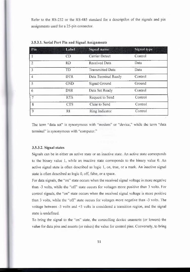
Refer to the RS-232 or the RS-485 standard for a description of the signals and pin

assignments used for a 25-pin connector.

3.5.3.1. Serial Port Pin and Signal Assignments

Pin Label Signal name Signal type

1 CD Carrier Detect Control

2 RD Received Data Data

3 TD Transmitted Data Data

4 DTR Data Terminal Ready Control

5 GND Signal Ground Ground

6 DSR Data Set Ready Control

7 RTS Request to Send Control

8 CTS Clear to Send Control

. 9 RI Ring Indicator Control

The term "data set" is synonymous with "modem" or "device," while the term "data

terminal" is synonymous with "computer."

3.5.3.2. Signal states

Signals can be in either an active state or an inactive state. An active state corresponds

to the binary value 1, while an inactive state corresponds to the binary value 0. An

active signal state is often described as logic 1, on, true, or a mark. An inactive signal

state is often described as logic 0, off, false, or a space.

For data signals, the "on" state occurs when the received signal voltage is more negative

than -3 volts, while the "off'' state occurs for voltages more positive than 3 volts. For

control signals, the "on" state occurs when the received signal voltage is more positive

than 3 volts, while the "off" state occurs for voltages more negative than -3 volts. The

voltage between -3 volts and + 3 volts is considered a transition region, and the signal state is undefined.

To bring the signal to the "on" state, the controlling device unasserts (or lowers) the

value for data pins and asserts (or raises) the value for control pins. Conversely, to bring

51

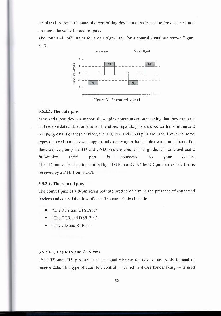
the signal to the "off' state, the controlling device asserts the value for data pins and

unasserts the value for control pins.

The "on" and "off' states for a data signal and for a control signal are shown Figure

3.13. Data Signal Control Signal

6

--- -~- 1 -~_] .• c------ ___ -----

-6

Figure 3.13: control signal

3.5.3.3. The data pins

Most serial port devices support full-duplex communication meaning that they can send

and receive data at the same time. Therefore, separate pins are used for transmitting and

receiving data. For these devices, the TD, RD, and GND pins are used. However, some

types of serial port devices support only one-way or half-duplex communications. For

these devices, only the TD and GND pins are used. In this guide, it is assumed that a

full-duplex serial port is connected to your device.

The TD pin carries data transmitted by a DTE to a DCE. The RD pin carries data that is

received by a DTE from a DCE.

3.5.3.4. The control pins

The control pins of a 9-pin serial port are used to determine the presence of connected

devices and control the flow of data. The control pins include:

• "The RTS and CTS Pins"

• "The DTR and DSR Pins"

• "The CD and RI Pins"

3.5.3.4.1. The RTS and CTS Pins.

The RTS and CTS pins are used to signal whether the devices are ready to send or

receive data. This type of data flow control - called hardware handshaking - is used

52

• to prevent data loss during transmission. When enabled for both the DTE and DCE,

hardware handshaking using RTS and CTS follows these steps:

1. The DTE asserts the RTS pin to instruct the DCE that it is ready to receive data.

2. The DCE asserts the CTS pin indicating that it is clear to send data over the TD

pin. If data can no longer be sent, the CTS pin is unasserted.

3. The data is transmitted to the DTE over the TD pin. If data can no longer be

accepted, the RTS pin is unasserted by the DTE and the data transmission is

stopped.

3.5.3.4.2. The DTR and DSR Pins.

Many devices use the DSR and DTR pins to signal. if they are connected and powered.

Signaling the presence of connected devices using DTR and DSR follows these steps:

1. The DTE asserts the DTR pin to request that the DCE connect to the

communication line.

2. The DCE asserts the DSR pin to indicate that it is connected.

3. DCE unasserts the DSR pin when it is disconnected from the communication

line.

The DTR and DSR pins were originally designed to provide an alternative method of

hardware handshaking. However, the RTS and CTS pins are usually used in this way,

-and not the DSR and DTR pins. However, you should refer to your device

documentation to determine its specific pin behavior.

3.5.3.4.3. The CD and RI Pins.

The CD and RI pins are typically used to indicate the presence of certain signals during

modem-modem connections. CD is used by a modem to signal that it has made a

connection with another modem, or has detected a carrier tone. CD is asserted when the

DCE is receiving a signal of a suitable frequency. CD is unasserted if the DCE is not

receiving a suitable signal. RI is used to indicate the presence of an audible ringing

signal. RI is asserted when the DCE is receiving a ringing signal. RI is unasserted when

the DCE is not receiving a ringing signal (for example, it's between rings).

53

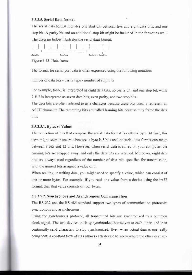
3.5.3.5. Serial Data format •

The serial data format includes one start bit, between five and eight data bits, and one

stop bit. A parity bit and an additional stop bit might be .included in the format as well.

The diagram below illustrates the serial data format.

Start bit Data hits Parity hit Stop bits

Figure 3.13: Data frame

The format for serial port data is often expressed using the following notation:

number of data bits - parity type - number of stop bits

For example, 8-N-1 is interpreted as eight data bits, no parity bit, and one stop bit, while

7-E-2 is interpreted as seven data bits, even parity, and two stop bits.

The data bits are often referred to as a character because these bits usually represent an

ASCII character. The remaining bits are called framing bits because they frame the data

bits.

3.5.3.5.1. Bytes vs Values

The collection of bits that compose the serial data format is called a byte. At first, this

term might seem inaccurate because a byte is 8 bits and the serial data format can range

between 7 bits and 12 bits. However, when serial data is stored on your computer, the

framing bits are stripped away, and only the data bits are retained. Moreover, eight data

bits are always used regardless of the number of data bits specified for transmission,

with the unused bits assigned a value of 0.

When reading or writing data, you might need to specify a value, which can consist of

one or more bytes. For example, if you read one value from a device using the int32

format, then that value consists of four bytes.

3.5.3.5.2. Synchronous and Asynchronous Communication

The RS-232 and the RS-485 standard support two types of communication protocols:

synchronous and asynchronous.

Using the synchronous protocol, all transmitted bits are synchronized to a common

clock signal. The two devices initially synchronize themselves to each other, and then

continually send characters to stay synchronized. Even when actual data is not really

being sent, a constant flow of bits allows each device to know where the other is at any

54

given time. That is, each bit that is sent is either actual cfata or an idle character.

Synchronous communications allows faster data transfer rates than asynchronous

methods, because additional bits to mark the beginning and end of each data byte are

not required.

Using the asynchronous protocol, each device uses its own internal clock resulting in

bytes that are transferred at arbitrary times. So, instead of using time as a way to

synchronize the bits, the data format is used.

In particular, the data transmission is synchronized using the start bit of the word, while

one or more stop bits indicate the end of the word. The requirement to send these

additional bits causes asynchronous communications to be slightly slower than

synchronous. However, it has the advantage that the processor does not have to deal

with the additional idle characters. Most serial ports operate asynchronously.

3.5.3.5.3. How Are the Bits Transmitted?

By definition, serial data is transmitted one bit at a time. The order in which the bits are

transmitted follows these steps:

I. The start bit is transmitted with a value of 0.

2. The data bits are transmitted. The first data bit corresponds to the least

significant bit (LSB), while the last data bit corresponds to the most significant

bit (MSB).

3. The parity bit (if defined) is transmitted.

4. One or two stop bits are transmitted, each with a value of I.

The number of bits transferred per second is given by the baud rate. The transferred bits

include the start bit, the data bits, the parity bit (if defined), and the stop bits.

3.5.3.5.4. Start and Stop bits

Most serial ports operate asynchronously. This means that the transmitted byte must be

identified by start and stop bits. The start bit indicates when the data byte is about to

begin and the stop bit(s) indicates when the data byte has been transferred. The process

of identifying bytes with the serial data format follows these steps:

I. When a serial port pin is idle (not transmitting data), then it is in an "on" state.

2. When data is about to be transmitted, the serial port pin switches to an "off'

state due to the start bit.

3. The serial port pin switches back to an "on" state due to the stop bit(s). This

indicates the end of the byte. 55

•

The data bits transferred through a serial port might represent device commands, sensor

readings, error messages, and so on. The data can be transferred as either binary data or

as text (ASCII) data.

Most serial ports use between five and eight data bits. Binary data is typically

transmitted as eight bits. Text-based data is transmitted as either seven bits or eight bits.

If the data is based on the ASCII character set, then a minimum of seven bits is required

because there are 27 or 128 distinct characters. If an eighth bit is used, it must have a

value of 0. If the data is based on the extended ASCII character set, then eight bits must

be used because there are 28 or 256 distinct characters.

3.5.3.5.6. The parity bit

The parity bit provides simple error (parity) checking for the transmitted data. The types

of parity checking are given below.

Parity type Description

Even The data bits plus the parity bit produce an even number of 1 s.

Mark The parity bit is always 1.

Odd The data bits plus the parity bit produce an odd number of ls.

Space The parity bit is always 0.

Mark and space parity checking are seldom used because they offer minimal error

detection. You might choose not to use parity checking at all.

The parity checking process follows these steps:

1. The transmitting device sets the parity bit to O or to 1 depending on the data bit

values and the type of parity checking selected.

2. The receiving device checks if the parity bit is consistent with the transmitted

data. If it is, then the data bits are accepted. If it is not, then an error is returned.

3.5.4. Configuring Communication Settings I MATLAB

3.5.4.1. Creating a Serial Port Object

You create a serial port object with the serial function. Serial requires the name of the

serial port connected to your device as an input argument. you can also configure

property values during object creation.

56

Before you can write or read data, both the serial port object and the instrument must

have identical communication settings. Configuring serial port communications

involves specifying values for properties that control the baud rate and the "Serial Data

Format" These properties are as follows.

Property Name Description

BaudRate Specify the rate at which bits are transmitted.

DataBits Specify the number of data bits to transmit.

Parity Specify the type of parity checking.

StopBits Specify the number of bits used to indicate the end of a byte.

Terminator Specify the terminator character.

3.5.5. Interfacing Devices to RS-232 Ports

3.5.5.1. RS-232 Waveforms

So far we have introduced RS-232 Communications in relation to the PC. RS-232

communication is asynchronous. That is a clock signal is not sent with the data. Each

word is synchronized using it's start bit, and an internal clock on each side, keeps tabs

on the timing.

:::: ::: l Sbrt I O I 1 I 2 I J I 4 I S I 6 I 7 I Stop L +:: Figure 3.14: TTL/CMOS Serial Logic Waveform

The diagram above, shows the expected waveform from the UART when using the

common 8Nl format. 8Nl signifies 8 Data bits, No Parity and 1 Stop Bit. The RS-232

line, when idle is in the Mark State (Logic 1). A transmission starts with a start bit

which is (Logic 0). Then each bit is sent down the line, one at a time. The LSB (Least

Significant Bit) is sent first. A Stop Bit (Logic 1) is then appended to the signal to make

up the transmission.

The diagram, shows the next bit after the Stop Bit to be Logic 0. This must mean

another word is following, and this is it's Start Bit. If there is no more data coming then

the receive line will stay in it's idle state(logic 1 ). We have encountered something

called a "Break" Signal. This is when the data line is held in a Logic O state for a time

57

long enough to send an entire word. Therefore if you don't put' the line back into an idle

state, then the receiving end will interpret this as a break signal.

The data sent using this method, is said to be framed. That is the data is framed between

a Start and Stop Bit. Should the Stop Bit be received as a Logic 0, then a framing error

will occur. This is common, when both sides are communicating at different speeds.

The above diagram is only relevant for the signal immediately at the UART. RS-232

logic levels uses +3 to +25 volts to signify a "Space" (Logic 0) and -3 to -25 volts for a

"Mark" (logic 1). Any voltage in between these regions (ie between +3 and -3 Volts) is

undefined. Therefore this signal is put through a "RS-232 Level Converter". This is the

signal present on the RS-232 Port of your computer, shown in figure 3.15.

Mark

Space

Figure 3.15: RS-232 Logic Waveform

The above waveform applies to the Transmit and Receive lines on the RS-232 port.

These lines carry serial data, hence the name Serial Port. There are other lines on the

RS-232 port which, in essence are Parallel lines. These lines (RTS, CTS, DCD, DSR,

DTR, RTS and RI) are also at RS-232 Logic Levels.

3.5.5.2. RS-232 Level Converter

Almost all digital devices which we use require either TTL or CMOS logic levels.

Therefore the first step to connecting a device to the RS-232 port is to transform the RS-

232 levels back into O and 5 Volts. As we have already covered, this is done by RS-232

Level Converters.

58

---

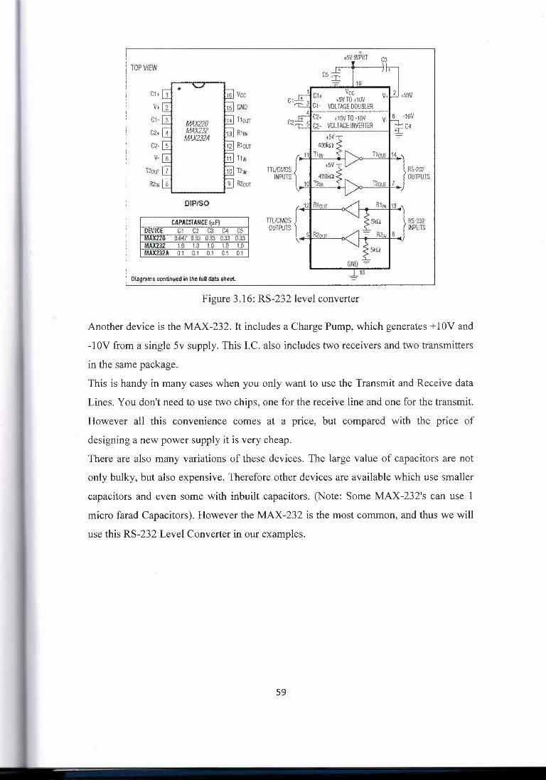
10PV!EW

•

MAY.220 !A4X232 MAX232A

DIP/SO

CAPACIT AflCE (µFl DEVICE C1 C2 C3-C4 -Ci; MAX220 OJM7 0.33 0.33 0.33 033 MAX232 tO LO to 1.0 t.O MAX23eA OJ OJ OJ 0.1 O.t

Dlagr~ms continued in the full d3ta $heet

• +5V INPUT cs JT···"···---3f:ri

C5T I

a. = Vcc16 ,j , c1 Ch ,5V TO +!OV V+ --- ,10V

, G1- \iOLTAGEOOUBLER ----~--- .....•....... -, ' __F"" C2+ +1GVTO-HN V- 6 -10\f

G2= C2- VO!.TAGE.INVERTER ~ C4 :;::r::: .

400~;~ 11 T1m <

nw,os[ "'j INPUTS I ~rn r:1!00'~1 £.

\.'

J21 Rlorn TIUGMOS r (JlJTP!JTS l . gl R2nm

\

R,~a,13} RS-232 5hll

I

INPUTS

= Figure 3.16: RS-232 level converter

Another device is the MAX-232. It includes a Charge Pump, which generates + 1 OV and -1 OV from a single 5v supply. This LC. also includes two receivers and two transmitters

in the same package.

This is handy in many cases when you only want to use the Transmit and Receive data

Lines. You don't need to use two chips, one for the receive line and one for the transmit.

However all this convenience comes at a price, but compared with the price of

designing a new power supply it is very cheap.

There are also many variations of these devices. The large value of capacitors are not

only bulky, but also expensive. Therefore other devices are available which use smaller

capacitors and even some with inbuilt capacitors. (Note: Some MAX-232's can use 1

micro farad Capacitors). However the MAX-232 is the most common, and thus we will

use this RS-232 Level Converter in our examples.

59

• 3.5.6. FTDI Chip

FTDI (Future Technology Devices International) Chip offers a wide range of products

including modules, cables, and integrated circuits. Driven by its chip development,

FTDI's product focus is on USB connectivity and display interfaces, which have wide

applications across all market segments, including; industrial, consumer, PC peripheral,

medical, telecom, energy infrastructure, etc.

60

•

Chapter 4 Practical results- MATLAB/Arduino/Solar tracking system

4.1.Practical prototype In the prototype we used Arduino board with motor shield to determine the angle of solar cell in order to be orthogonal with the sun light. For that i used light sensor (LDR) to detect the sun position and give the motor the rotate commands, figure 4.1.

Figure 4.1: Practical prototype

4.2.Control Methods Many methods could be applied in this project to track the sun lights, each method has its own properties. The most used methods are:

Traditional control method. Sun position (zenith - azimuth). PID control. Fuzzy control.

In my project I applied the first three methods using two techniques:

Programing environment. Simulink environment.

61

4.2.1. Programming environment

4.2.1.1. Traditional control method.

•

62

--~- ·-------- ----

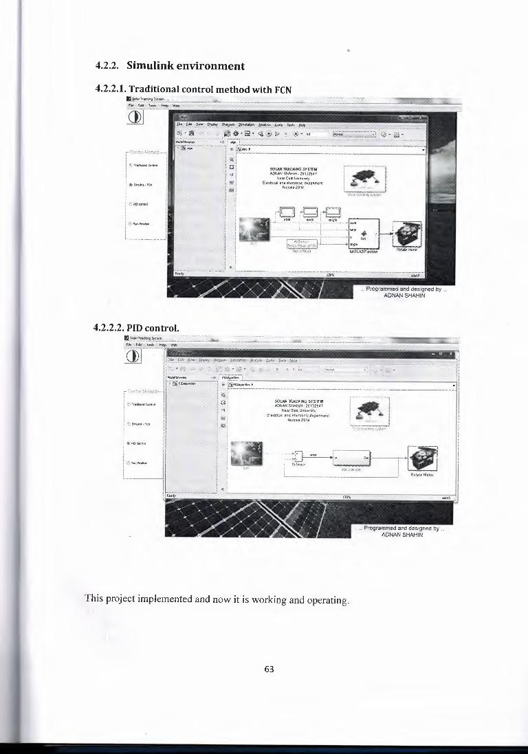
• 4.2.2. Simulink environment

4.2.2.1. Traditional control method with FCN

4.2.2.2. PID control.

SOLAR lRACKING &YS1EM ~DNAN SHA.'-liN -2~13:2~47

N!:uEast.Urfr,ersity f!e:<:tric.aJ ande:!l(!,ct<t<llkd&part.eI,~!11.

-Nica°9B2014

This project implemented and now it is working and operating.

63

References • 1. Erinmez, I.A., Bickers, D.O.,Wood, G.F. and Hung,W.W. (1999) NGC Experience

with frequency control in England and Wales: provision of frequency response by generator. IEEE PES Winter Meeting, 31 January-4 February 1999, New York, USA.

2. European Commission (2006) European SmartGrids Technology Platform:Vision and Strategy for Europe's Electricity, http://ec.europa.eu/research/ energy /pdf/ smartgrids _ en. pdf ( accessed on 4 August 2011).

3. Department of Energy and Climate Change, UK, Smarter Grids: The Opportunity,December 2009, http://www.decc.gov. uk/ assets/ decc/what%20we%20do/uk%20energy%2 Osupply /fu tureelectricitynetworks/1 _ 20091203163757 _ e _@@_ smartergridsopportunity.pdf (accessed on 4 August 2011).

4. U.S. Department of Energy, Smart Grid System Report, July 2009, http://www.oe.energy.gov I sites/prod/files/ oeprod/DocumentsandMedia/SGSRMain _ 090707 _lowres.pdf (accessed on 4 August 2011 ).

5. World Economic Forum (2009) Accelerating Smart Grid Investments, http://www.weforum.org/pdf/SlimCity/SmartGrid2009.pdf (accessed on 4 August 2011).

6. Pudjianto, D., Ramsay, C. and Strbac, G. (2007) Virtual power plant and system integration of distributed energy resources. Renewable Power Generation, IET, 1 (1),10-16.

7. Gellings, C.W. (2009) The Smart Grid: Enabling Energy Efficiency and Demand Response, The Fairmont Press, Lilburn.

8. Galvin, R., Yeager, K. and Stuller, J. (2009) Perfect Power: How the Microgrid Revolution Will Unleash Cleaner, Greener, More Abundant Energy, McGraw-Hill, New York.

9. The Integrated Energy and Communication Systems Architecture, 2004, http://www.epriintelligrid.com/intelligrid/docs/IECSA _ Volume!. pdf ( accessed on 4 August 2011).

10. XCel Energy Smart Grid: A White Paper, March 2007, http://smartgridcity.xcelenergy.com/media/pdf/SmartGridWhitePaper.pdf (accessed on 4 August 2011).

11. Southern California Edison Smart Grid Strategy and Roadmap, 2007 ,http://asset.sce.com/Documents/Environment%20%20Smart%20Grid/l 00712 _ SCE _SmartGridStrategyandRoadmap.pdf (accessed on 4 August 2011).

12. Arrillaga, J. (1998) High Voltage Direct Current Transmission, IET, Stevenage. Kim, C., Sood, V.K. and Seong-Jo, G.J. (2010) HVDC Transmission: Power Conversion Applications in Power Systems, Wiley-IEEE, Singapore.

14. Barker, C. et al. (2010) HVDC: Connecting to the Future, Alstom Grid. 15. Song, Y.H. and Johns, A.T. (1999) Flexible AC Transmission Systems, IET Power

and Energy Series 30. 16. Acha, E., Fuerte-Esquivel, C.R., Ambriz-P 'erez, H. and Angeles-Camacho,(2004)

FACTS: Modelling and Simulation in Power Networks, John Wiley & Sons Ltd, Chichester.

17. Jenkins, N., Ekanayake, J.B. and Strbac, G. (2010) Distributed Generation, IET, Stevenage.

18. Heier, S. (2006) Grid Integration of Wind Energy Conversion Systems, John Wiley & Sons, Ltd, Chichester.

64

- ---·-

19. Anaya-Lara, 0., Jenkins, N., Ekanayake, J. et al. (2009) Wind Energy Generation: Modelling and Control, John Wiley & Sons, Ltd, Chichester.

20. Hingorani, H. (1995) Introducing custom power. IEEE Spectrum, 32(6), 41-48. 21. Mohan, N., Undeland, T.M. and Robbins, W.P. (1995) Power Electronics:

Converters,Applications and Design, John Wiley & Sons, Inc, New York. 22. Yazdani, A. and Iravani, R. (2010) Voltage-Sourced Converters in Power

Systems, IEEEWiley, Singapore. 23. Holtz, J. (1992) Pulsewidth modulation - a survey. IEEE Transactions on

Industrial Electronics, 39(5), 410-420. 24. Handley, P.G. and Boys, J.T. (1992) Practical real-timePWMmodulators: an

assessment. IEE Proceedings-B (Electric Power Applications), 139(2), 96-102. 25. Shen, J. and Butterworth, N. (1997) Analysis and design of a three-level

PWMconverter system for railway-traction applications. IEE Proceeding Electric Power Applications, 144(5), 357-371.

26. Nabae, A., Takahashi, I. and Akagi, H. (1981) A new neutral-point-clamped PWM inverter. IEEE Transactions on Industry Applications, lA-17(5), 518-523.

27. Withanage, R., Crookes,W. and Shammas, N. (2007) Novel voltage balancing technique for series connection of IGBTs. 2007 European Conference on Power Electronics and Applications, 2007, pp. 1-10.

28. Hochgraf, C., Lasseter, R., Divan, D. and Lipo, T.A. (1994) Comparison of multilevel inverters for Static V Ar Compensation. IEEE Industry Applications .Society Annual Meeting, Vol. 2, 1994, pp. 921-928.

65