national oceanic and atmospheric administration national weather
TRANSCRIPT
U.S. DEPARTMENT OF COMMERCENATIONAL OCEANIC AND ATMOSPHERIC ADMINISTRATION
NATIONAL WEATHER SERVICENATIONAL METEOROLOGICAL CENTER
OFFICE NOTE 394
THE NMC ETA MODEL POST PROCESSOR:A DOCUMENTATION
RUSSELL TREADON
JUNE 1993
THIS IS AN INTERNALLY REVIEWED MANUSCRIPT,PRIMARILY INTENDED FOR INFORMAL EXCHANGE OF INFORMATION
AMONG NMC STAFF MEMBERS

Table of Contents
1. Introduction 1
2. The Eta Model 13. The Eta Post Processor - An Overview 54. The Eta Post Processor- Details 7
4.1 Sea level pressure 84.2 Subterranean fields 104.3 Constant eta and pressure fields 104.4 Tropopause level data 124.5 FD level fields 124.6 Freezing level data 134.7 Sounding fields 134.8 Surface based fields. 154.9 10m winds and 2m temperatures 164.10 Boundary layer fields 174.11 LFM and NGM look-alike fields 18
5. Summary 196. References 207. Appendix 1: Fields Posted from the Operational Eta 22
7.1 Discussion 227.2 Table 1. Where is it? 247.3 Table 2. Contents of Operational Eta Sequential Access, VSAM, 25
and GRIB I Files7.4 Table 3. Contents of Operational Eta Rotating Archives 277.5 Table 4. Contents of Operational Eta PC-Grids Files 287.6 Table 5. Office Note 84 Labels of Posted Eta Fields 297.7 Table 6. Eta based products 31
8. Appendix 2: Using the Eta Post Processor 348.1 Introduction 348.2 Namelist FCSTDATA 348.3 The Control File 348.4 The Template 398.5 Pre-computed Interpolation Weights 418.6 Internal and External Post 418.7 Summary 42
1. Introduction
This Office Note describes the post processor for the National Meteorological Center Eta model. Preliminary
to this discussion is a brief review of the Eta model emphasizing the model grid and arrangement of variables.
A general overview of the post processor design, usage, and capabilities follows. Currently 110 unique fields
are available from the post processor. The final section documents these fields and the algorithms used to
compute them. Appendix 1 lists the various NMC data sets from which operational Eta model output is avail-
able. Details for using the post processor in conjunction with the model are found in Appendix 2.
The Eta post processor is not a stagnant piece of code. New output fields, improved algorithms, GRIB pack-
ing, and code optimization are just a few areas in which development continues. However, it is unlikely that
the algorithms discussed in this Office Note will dramatically change.
2. The Eta Model
Since its introduction by Philips (1957) the terrain-following sigma coordinate has become the vertical coor-
dinate of choice inmostnumerical weather prediction models. Aprime reason for thsis is simplification of the
lower boundary condition. Difficulties arise in the sigma coordinate when dealing with steep terrain. In such
situations the noncancellation of errors in two terms of the pressure gradient force becomes significant (Sma-
gorinsky et aL, 1967). These errors in turn generate advection and diffusion errors. Numerous methods have
been devised to account for this defect of the sigma system. Mesinger (1984) took a different approach in
defining the eta coordinate,
r = P -- Pt x 7,
where
p(zs) - Ptf7S, p(o) - Pt
In this notation p is pressure and subscripts rf, s, and t respectively refer to reference pressure, the model
surface, and the model top (p, = 50 mb). The height zis geometric height. Observe that the sigma coordinate
appears as the q, = 1 case of the eta coordinate. The reference pressure used in the Eta model is
_ To -Fz\1n RpJz) = PA 0) ( T ) where p,(0) = 1013.25mb, To = 288K, F = 6.5°/kin, i = -g-, g = 9.80n/s2,
and R = 287.04J/Kkg.
l
In the eta coordinate terrain assumes a step-like appearance thereby minimizing problems associated with
steeply sloping coordinate surfaces. At the same time the coordinate preserves the simplified lower boundary
condition of a terrain following vertical coordinate.
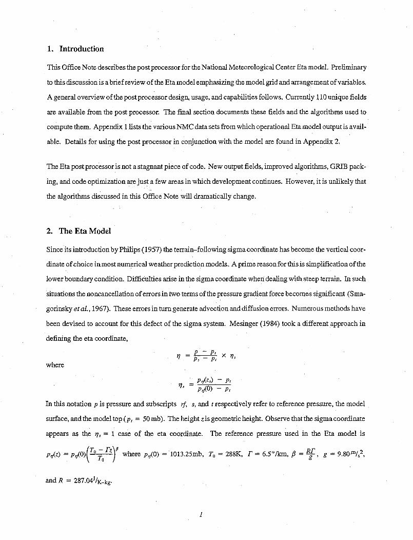
The Eta model uses the semi-staggered Arakawa E grid (Fig. 1). Prognostic variables at mass (H) points are
surface pressure, temperature, and specific humidity. Zonal and meridional wind components are carried at
velocity (V) points. The E grid is mapped to a rotated latitude-longitude grid which is centered at 52N and
111W for the operational Eta. Two rotations are involved. One moves the Greenwich meridian to 111W. The
second shifts the equator to 52N. Each row of the E grid lies along a line of constant rotated latitude; each
column along a line of constant rotated longitude. In the operational Eta the shortest distance between like
grid points is approximately 80 km. The large box in Fig. 1 delimits the extent of the computational domain.
Prognostic variables on the outermost rows and columns are specified by a global model forecast from the
previous cycle. The second outermost rows and columns serve to smoothly blend boundary conditions with
values in the computational domain. The boundaries are one way interactive.
H VH VH VH VH VHV H V H V H V H V H V
H V H V H V H VH VH
V H V H VH VH V H V
H V H V H x H H V H
-V H V v H V H V H V
H VH V V H V H V H
VH V H V H V H V H V
H VH VH VH V H VH
Fig. 1. Arakawa E grid of Eta model. H denotes mass points, V velocity points. Thesolid box outlines the computational domain. The distance d between like grid points isapproximately 80 km. The dashed box represents a model step.
Model terrain is represented in terms of discrete steps. Each step is centered on a mass point with a velocity
point at each vertex. This is suggested by the dashed box in Fig. 1. The algorithm creating the steps tends to
2

maximize their heights (so-called silhouette topography) based on the raw surface elevation data. Topogra-
phy over the operational Eta domain is discretized into steps from sea level to 3264 meters over the Colorado
Rockies. Figure 2 represents these steps on a bar chart.
3300
3000 M2700 .. ...2400 .MM MR .m
2100 .M. Mr MM
600 i~~~~~~~~~~~~~~~~~~~~$ MM S smsm ORMM MAMMNMZSC
1800 M mm.......M'
1M2 3 4 5 6 7 8 9 10 11 12 13 14 15 16 17 18 19Discrete steps in eta topographyFig. 2. Schematic of step topography used in operational Eta model. The top of each step coin-
cides with an interface between eta layers. Note that the thickness of eta layers increases moving
up from mean sea level.
00The operational Eta runs with 38 vertical layers. The thickness of the layers varies with greatest vertical reso-
300 M WM$ M Z
1 2 3 4 5 6 7 8 9 10 11 12~~~M 13 14 15 16 17 1IN 19
lution n ear seatlevel anp usd n250 mb (to better resolve jet dynaics). The top of each step coincides exact-
up from mean sea level.~~~~~~~~~~~~~~~~~~~~~~~~~~~~~~~~~~~~~~~~~~~~~~~~~~~~~~~~~~~~~~~~~~~~~~~~~~~~~~~~~~~~~~~~~~~~~~~~~~~~~~~~~~~~~~~~~~~~~~~~~~~~~~~~~~~~~~~~~~~~~~~~~~~~~~~~~~~~~~~~~~~~~~~~Ma M ~
ly with one of the interfaces between the model's layers. Note that the thickness of the lowest eta layer above
the model terrain is not horizontally homogeneous. This presents difficulties when posting terrain following
fields. Such fields often exhibit strong horizontal gradients in mountainous regions. Vertical averaging over
several eta layers, sometimes coupled with horizontal smoothing, minimizes this effect.
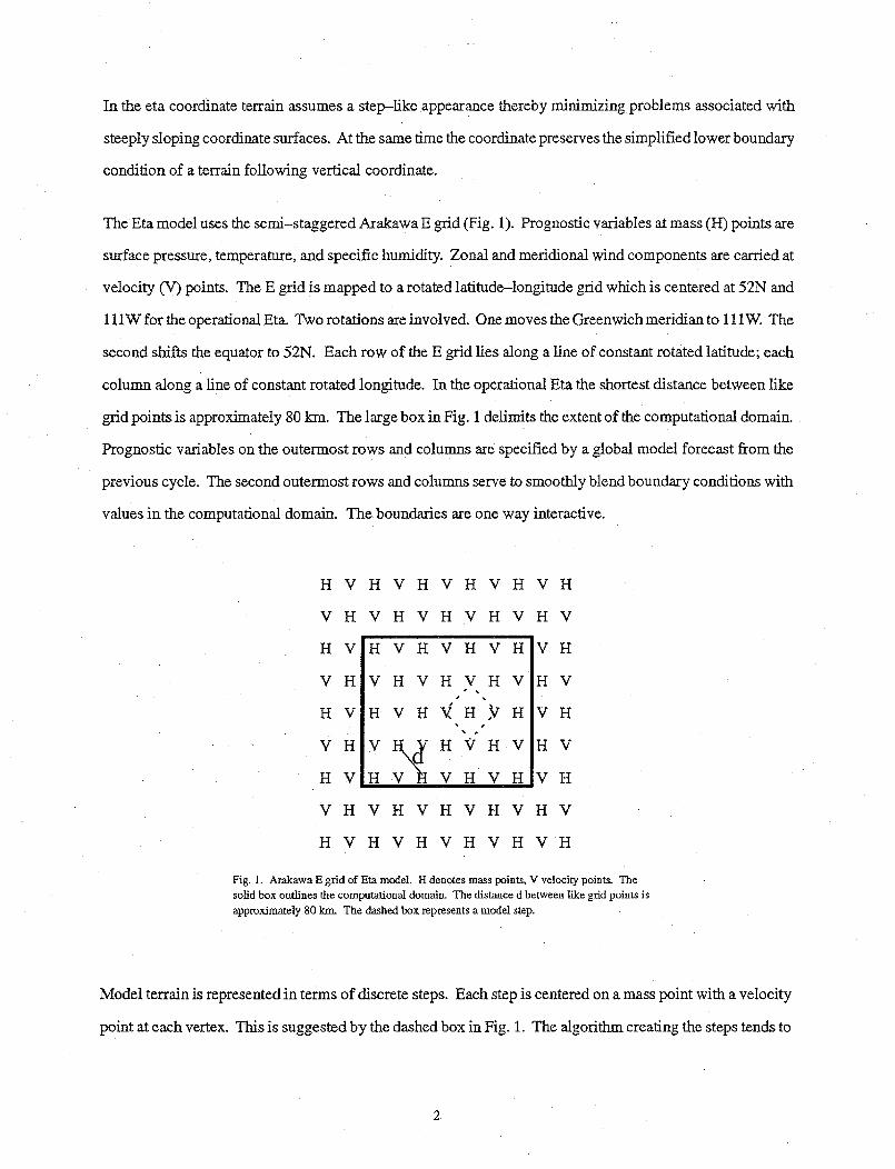
Model variables are staggered vertically as well as horizontally (Fig. 3). Temperature, specific humidity, and
wind components are computed at the midpoint of eta layers. Turbulent kinetic energy is defined at the inter-
faces between layers Ano-slip boun dary condition maintains z ero wind components along the side of steps.
Zero wind points are circled in Fig. 3.
The model uses a technique for preventing grid separation (Mesinger 1973, Janjie 1974) in combination with
the split-explict time differencing scheme (Mesinger 1974, Janjit 1979). The fundamental time step for the
operational Eta model is 200 seconds. This is the mass-momentum adjustment time scale. Advection, physi-
3
- u - ~~ ~ ~ ~ ~ ~ ~ ~ ~ ~ ~ ~ ~~-u .. - -'h- l,¼ '| H I- ' -u-v- * -,q- ',- -T.q- -u.v- '- U -.J * : I , , ,/
. , I ' I I I * . , ,
* I I ; I I I I I I I I
~'~ - Vrq --,- q - - -V,, - -~q- :- - - -U,-V -,- -rq-. - ' _ ' vP~~| | ~, -,' ---; v ,
Fig 3. Vetia crs eto hog t oeihMlyr. Teprape spcii huiiy .oa and
'~~~~~~~~~~~~~~~~~~~~~-~ i q _ ~a 3
mio w in I Ieo o e
e ho l a n a, , t , 1 Vr-2#. ~s g- Uff, -- Cjq T z )~-7tq~-M -T >-Fq - - U V
mV~~~~~~~~~~~~~~ I
I_ *! W I I I . I
tical adv 3 Vrtcacos ection ofmituei rbsdong Ethe pideewise-linears. Tmperthod, (Capentrc eutidi, 1989).an
lDS M5M 55 ACM 5WX~. f5~, .. ~
Leve 2.5schmeriinlwn (M orpoand s Yamadan1974, 1982iel) inrte dfrnee atmos ipher ofeathet M aellr-YaadP Leel2s
scheme forthe "surface" laysr Tecr, and awisdcous nsublayer over thde oseans (Zeideitinky evitsspchf170) Sufcepo
|~~~~~~~~~~~~~~~~~~~ ~/ w_ n5kz - - -... ~--,- q- -- ucv0~r -z- -JV -U prcessesaremoeled rafatie ose maof yo an th e stdel wSith is (19) emranud ueridsicf (t18 Duniaffuto tiles an
The horizontal advection algorithm has abuilt-in strictnonlinear energy cascade control (Janjic ,1984). Ver-
tical advection of moisture is based on the piecewise-linear method (Carpenter et al., 1989).
The model includes a fairly sophisticated physics package (Janjic', 1990) corisisting of the Mellor-Yamada
Level 2.5 scheme (Mellor and Yamada-1974, 1982) in the free atmosphere, the Mellor-Yamada Level 2.0
scheme for the "surface" layer, and a viscous sublayer over the oceans (Z:ilitinkevitch, 1970). Surface pro-
cesses are modeled after those of Miyakoda and Sirutis (1984) and Deardorff (1978). Diffusion utilizes a
second order scheme with the diffusion coefficient depending on turbulent kinetic energy and deformation of
the wind field. Large scale and parameterized deep and shallow convection are based on an approach pro-
posedby Betts (1986) and Betts and Miller (1986). The radiationis the NMC version of the GFDL radiation
scheme with interactive random overlap clouds.
4
The operational Eta runs from a static analysis based on Optimum Interpolation. First guess for the static
analysis comes from the T-126 Global Data Assimilation System (approximately 105 km horizontal resolu-
tion). An assimilation system directly on the E grid is being developed and research is ongoing towards an
adjoint Eta-based assimilation system. Boundary conditions for the model are provided by the previous
cycle global model forecast, again, at T-126 resolution.
A more complete treatment of the Eta model is found in Black (1988) and Black (1993). The presentation
above was intended to give the reader a general impression of the Eta model prior to discussing the Eta post
processor below.
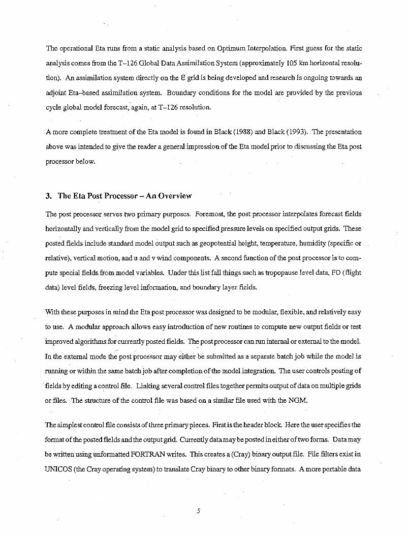
3. The Eta Post Processor - An Overview
The post processor serves two primary purposes. Foremost, the post processor interpolates forecast fields
horizontally and vertically from the model grid to specified pressure levels on specified output grids. These
posted fields include standard model output such as geopotential height, temperature, humidity (specific or
relative), vertical motion, and u and v wind components. A second function of the post processor is to com-
pute special fields from model variables. Under this list fall things such as tropopause level data, FD (flight
data) level fields, freezing level information, and boundary layer fields.
With these purposes in mind the Eta post processor was designed to be modular, flexible, and relatively easy
to use. A modular approach allows easy introduction of new routines to compute new output fields or test
improved algorithms for currently posted fields. The post processor can run internal or external to the model.
In the external mode the post processor may either be submitted as a separate batch job while the model is
running or within the same batch job after completion of the model integration. The user controls posting of
fields by editing a control file. Linking several control files together permits output of data on multiple grids
or files. The structure of the control file was based on a similar file used with the NGM.
The simplest control file consists of three primary pieces. First is the header block. Here the user specifies the
format of the posted fields and the output grid. Currently data may be posted in either of two forms. Data may
be written using unformatted FORTRAN writes. This creates a (Cray) binary output file. File filters exist in
UNICOS (the Cray operating system) to translate Cray binary to other binary formats. A more portable data
5

format is Office Note 84 packing. Both operational and quasi-operational versions of the Eta model post
fields according to Office Note 84 specifications. GRIB posting directly from the post is under development
For the interim GRIB versions of the Office Note 84 packed model output are generated by a separate program
following execution of the post processor.
Data may be posted on the staggered E grid, a filled (i.e., regular) version of this grid, or any grid defined using
standard NMC grid specifications. All computations involving model output are done on the staggered mod-
el grid. Bilinear interpolationisusedto fill the staggered grid. Asecondinterpolationisrequiredtopostdata
on a regular grid other than the filled E grid. This interpolation is also bilinear. Those grid points to which it is
notpossible to bilinearlyinterpolate avalue to receive one oftwo values. A searchis made fromthe outermost
rows and columns of the output grid inward to obtain "known" values along the edge of the region to which
interpolation was possible. Having identified these values the algorithm reverses direction and moves out-
ward along each row and column. Grid points to which interpolation was not possible are set equal to the
"known" value along their respective row and column. If after this operation corner points on the output grid
do not have values they areassigned the field mean. Depending on the number of output fields requested the
calculation of interpolation weights can take more CPU time than does posting the fields. For this reason
interpolation weights may be pre-computed, saved, and read during post execution. The post retains the abil-
ity to compute these weights internally prior to posting any fields. A character flag in the header block con-
trols this feature. A second character flag allows fields on different output grids to be appended to the same
output file using the same or different data formats.
The second section of a control file lists available fields. By setting integer switches (0=off, 1=on) the user
selects the fields and levels of interest. The current post processor has 110 unique output fields, some on
multiple levels. Room exists for posting data on up to 60 vertical levels. In posting fields to an output grid
smoothing or filtering of the data may be applied at any of three steps in the posting process. Fields may be
smoothed on the staggered E grid, filtered on a filled E grid, or filtered on the output grid. Control of smooth-
ing or filtering is viainteger switches. Nonzero integers activate the smoother or filter with the magnitude of
the integer representing the number of applications (passes) of the selected smoother or filter. The smoother
coded in the post is a fourth order smoother which works directly on the staggered E grid. Once data is on a
regular grid a 25 point Bleck filter is available. A nice property of this filter is its fairly sharp response curve.
6
Repeated applications will remove wavelengths twice the grid spacing while largely preserving field minima
and maxima. Additional smoothing of posted fields can be realized in the interpolation process itself.
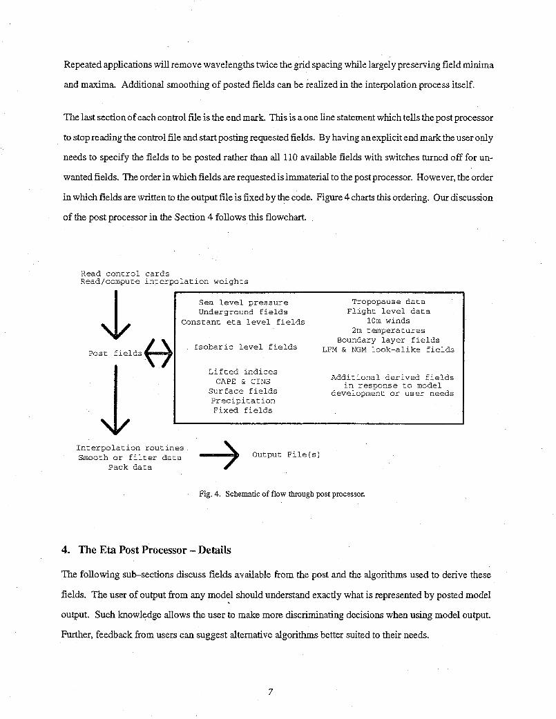
The last section of each control file is the end mark. This is a one line statement which tells the post processor
to stop reading the control file and start posting requested fields. By having an explicit end mark the user only
needs to specify the fields to be posted rather than all 110 available fields with switches turned off for un-
wanted fields. The order in which fields are requestedis immaterial to the postprocessor. However, the order
in which fields are written to the output file is fixed by the code. Figure 4 charts this ordering. Our discussion
of the post processor in the Section 4 follows this flowchart.
Read control cardsRead/compute interpolation weights
Post fields
\!/Interpolation routinSmooth or filter da
Pack data
Les
ta Output File(s)
Fig. 4. Schematic of flow through post processor.
4. The Eta Post Processor - Details
The following sub-sections discuss fields available from the post and the algorithms used to derive these
fields. The user of output from any model should understand exactly what is represented by posted model
output. Such knowledge allows the user to make more discriminating decisions when using model output.
Further, feedback from users can suggest alternative algorithms better suited to their needs.
7
Sea level pressure Tropopause dataUnderground fields Flight level data
Constant eta level fields 10m winds2m temperatures
Boundary layer fieldsIsobaric level fields LFM & NGM look-alike fields
Lifted indicesCAPEd ind s Additional derived fields
CAPE & CINS in response to modelSurface fields development or user needsPrecipitationFixed fields

4.1 Sea level pressure.
Sealevel pressure is one of the most frequently used fields posted from any operational model. Just as surface
pressure observations must be reduced to sea level so must forecast surface pressures be reduced to sea level.
The question here is which of a myriad of reduction algorithms to use. Different reduction algorithms can
produce significantly different sea level pressure fields given similar input data. The traditional approach is to
generate "representative" underground temperatures in vertical columns and then integrate the hydrostatic
equation downward. Saucier (1957) devotes several pages detailing the then current U.S. Weather Bureau
reduction scheme. Cram and Pielke (1989) compare and contrast two reduction procedures using surface
winds and pressure. References for other schemes may be found in their paper.
Sealevel pressure is available from the Eta model using either of two reduction algorithms. One is based on a
scheme devised by Mesinger (1990). The other is the "standard" NMC reduction algorithm. The methods
differ in the technique used to create fictitious underground temperatures.
The "standard" reduction algorithm uses the column approach of vertically extrapolating underground tem-
peratures from a representative above ground temperature. The algorithm starts with the hydrostatic equation
in the form
dz RdTy- d(ln(p)) g
where
z = geometric height,
p =air pressure,
T = virtual temperature (approximately given by T(1 + 0.608q); T, the dry air temperature and
q, the specific humidity,
Rd = dry air gas constant, and
g = gravitational acceleration.
Mean sea level pressure, p(msl), is computed at mass points using the formula p(msl) = p(sfc) x ef. The
function f = (i-f where r' is the average of r at the model surface and mean sea level. The remainingustion i h z(sfc) '
question is how to determine these r's.
8
In the NGM r(sfc) and r(msl) are first set using a 6.5°/kmn lapse rate from the first sigma layer. A similar ap-
proach was not successful in the Eta model due to the discontinuous nature of the step topography. Virtual
temperatures are averaged over eta layers in the first 60 mb above the model surface. The resulting layer mean
virtual temperature field is in turn horizontally smoothed before extrapolating surface and sea level tempera-
tures.
In both the NGM and Eta r(sfc) and r(msl) are subject to the Sheull correction. Whether this correction is
applied or not depends on the relation of the extrapolated r's to a critical value r, = Rd X 290.66.g
The Sheull correction is applied in two cases:
(1) When only r(ms/) exceeds rT,, set r(msr) to rcr,
(2) When both r(sfc) and r(msl) exceed r,, set r(msl) = r, - II(r(sfc) - r) 2 ,
where t = 0.005 x R
Once mean sea level pressure is computed a consistent 1000 mb height field is obtained using the relation
p(msl) - p(lOOOmb) = x z(1000 mb). This simple relationship itself can be used to obtain sea level
pressure given 1000 mb geopotential heights and an assumed mean density. In the post the mean density, e',
is computed from r'and p' (the average in log pressure of p(sfc) and p(msl)).
In contrast to the traditional column approach the Mesinger scheme uses horizontal interpolation to obtain
underground virtual temperatures. The argument here is that it is physically more reasonable to create under-
ground temperatures using atmospheric temperatures surrounding the mountain rather than extrapolating
downward from a single temperature on the mountain. The step-mountain topography of the Eta model sim-
plifies coding of this approach. The algorithm starts from the tallest resolved mountain and steps down
through the topography. Virtual temperatures on each step inside the mountain (i.,e., underground) are ob-
tained by solving a Laplace equation. Atmospheric virtual temperatures on the same step surrounding the
mountain provide consistent, realistic boundary conditions. Once all underground temperatures have been
generated the hydrostatic equation is integrated downward to obtain sea level pressure.
9
For selected sites the Eta model posts vertical profile (sounding) data plus several surface fields. The posting
of profile information is not part of the post processor. Sea level pressures included in the profile data are
available only from the Mesinger scheme. The standard and Mesinger schemes can produced markedly dif-
ferent sea level pressure fields given the same input data. This is especially true in mountainous terrain. The
Mesinger scheme generally produces a smoother analysis, much as one might produce by hand.
4.2 Subterranean fields.
Over large portions of the Eta domain mean sea level is below the model terrain; hence the need for the sea
level pressure reduction algorithms. Either algorithm generates underground temperatures and 1000 mb geo-
potential heights. Unresolved is the treatment of moisture and velocity fields below the model terrain. The
approach taken in the Eta post processor follows the NGM. In each vertical column the lowest atmospheric
eta layer relative humidity, zonal wind, meridional wind, and vertical motion fields are maintained below the
model terrain. That is, there is constant extrapolation of the lowest atmospheric eta layer fields below the
model surface. Underground specific humidity is adjusted to maintain the lowest atmospheric eta layer rela-
tive humidity given the underground temperatures generated by the sea level pressure reduction algorithm.
4.3 Constant eta and pressure fields.
Once underground temperature, humidity, and velocity fields have been specified there exists data on all eta
layers. Itis thenpossibleto output data on constant eta orpressure levels. For either option the fields that may
be posted are height, temperature (ambient, potential, and dewpoint), humidity (specific and relative), mois-
ture convergence, zonal and meridional wind components, vertical velocity, absolute vorticity, the geostroph-
ic streamfunction, and turbulent kinetic energy. Pressure may also be posted on constant eta layers.
Two options exist for posting eta layer data. Data may be posted from the n-th eta layer. This is simply a
horizontal slice through the three dimensional model grid along then-theta layer. The slice disregards model
topography. A second optionis to post fields on then-theta layer above the model surface. From the defini-
tion of the eta coordinate it is clear that an eta-based terrain following layer is generally not a constant mass
layer. In the current 38 layer operational Eta the thinnest first atmospheric eta layer is 20 meters thick while
the deepest such layer (over a few grid points in the Colorado Rockies) is 360 meters thick. Despite differ-
ences in layer thickness, examining data in the n-th atmospheric eta layer does have merit. It permits the user
10

to see what is truly happening in the n-th eta layer above the model surface and as such represents an eta-
based boundary layer perspective. Additionally, the code can post mass weighted fields in six 30 mb deep
layers stacked above the model surface (see Section 4.10). The operational Eta does not post eta layer data.
The more traditional way of viewing model output is on constant pressure surfaces. The post processor inter-
polates fields to nineteen isobaric levels (every 50 mb from 100 to 1000 mb). Vertical interpolation of temper-
ature, specific humidity, vertical velocity, and turbulent kinetic energy is quadratic in log pressure. For
horizontal and vertical winds the vertical interpolation is linear in log pressure. Consistent geopotential
heights are deduced by integrating the hydrostatic equation using interpolated temperatures and specific hu-
midity. Derived fields (e.g., dewpoint temperature, relative humidity, absolute vorticity, geostrophic stream-
function, etc.,) are computed from vertically interpolated base fields.
Still open is what to do if a requested isobaric level lies below the lowest model layer or above the model top
(50 mb). Vertical and horizontal wind components above the model top are a constant extrapolation of the
field at the uppermost model level. For isobaric levels below the lowest model layer the first atmospheric eta
layer fields are posted. Turbulent kinetic energy (TKE) is defined at model interfaces rather than the midpoint
of each layer. At isobaric layers above the model top the average TKE over the two uppermost model inter-
faces is constantly extrapolated. The same is done for pressure surfaces below the lowest model layer using
TKE from the two lowest above ground interfaces.
Temperature, humidity, and geopotential heights are treated differently. For pressure levels above the model
top the virtual temperature averaged over the two uppermost model layers is extrapolated assuming a standard
atmospheric lapse rate. The specific humidity at the target level is set so as to maintain the relative humidity
averaged over the two uppermost model layers. Geopotential heights are computed from the temperature and
specific humidity using the hydrostatic equation. The treatmentis the same for isobaric levels below the low-
est model layer except that the averaging is over fields in the second and third model layers above the surface.
Including data from the first atmospheric layer imposed a strong surface signature on the extrapolated isobar-
ic level data.
1I
4.4 Tropopause level data.
The post processor can generate the following tropopause level fields: pressure, temperature (ambient and
potential), horizontal winds, and vertical wind shear. The greatest difficulty was coding an algorithm to locate
the tropopause above each mass point. The procedure used in the Eta post processor is based on that in the
NGM. Above each mass point a surface-up searchis made for the first occurrence of two adjacent layers over
which the lapse rate is less than a critical lapse rate. In both the NGM and Eta model the critical lapse rate is
2K/kin. The midpoint (in log pressure) of these two layers is identified as the tropopause. A lower bound of
500 mb is enforced on the tropopause pressure. If no two layer lapse rate satisfies the above criteria the model
top is designated the tropopause. Very strong horizontal pressure gradients result from this algorithm. Hori-
zontal averaging over neighboring grid points prior to or during the tropopause search might minimize this
effect. To date this alternative has not been coded. It might be more accurate to describe the current algorithm
as one locating the lowest tropopause fold above 500 mb.
Linear interpolation in log pressure from the model layers above and below the tropopause provides the tem-
perature. Recall that velocity points are staggered with respect to mass points. Winds at the four velocity
points surrounding each mass point are averaged to provide a mass point wind. These mass point winds are
used in the vertical interpolation to tropopause level. Vertical differencing between horizontal wind fields
above and below the tropopause provides an estimate of vertical wind shear at the tropopause.
4.5 FD level fields.
Flight level temperatures and winds are posted at six levels, namely 914, 1524, 1829, 2134, 2743, and 3658
meters above the model surface. At each mass point a surface-up search is made to locate the model layers
bounding the target FD level height. Linear in log pressure interpolation gives the temperature at the target
height. Again, wind components at the four velocity points surrounding each mass point are averaged to pro-
vide a mass point wind. The wind averaging is coded so as to not include zero winds in the average. This can
happen in mountainous terrain where the no slip boundary condition of the model maintains zero winds along
the side of steps. Experimentation demonstrated that the averaging of winds to mass points minimized point
maxima or minima in posted FD level wind fields. This process is repeated for all six flight level heights.
12

4.6 Freezing level data.
The post processor computes freezing level heights and relative humidities at these heights. The calculation
is made at each mass point. Moving up from the model surface a search is made for the two model layers over
which the temperature first falls below 273.16 K. Vertical interpolation gives the mean sea level height, tem-
perature, pressure, and specific humidity at this level. From these fields the freezing level relative humidity is
computed. These fields are used to generate the FOUS 40-43 NWS bulletins containing six hourly forecasts
of freezing level heights and relative humidities for forecast hours twelve through forty-eight. The surface-
up search algorithm means posted freezing level heights can never be below the model terrain. This differs
from the LFM algorithm where underground heights were possible.
4.7 Sounding fields.
Several lifted indices are available from the Eta model. All are defined as being the temperature difference
between the temperature of a lifted parcel and the ambient temperature at 500 mb. The distinction between the
indices hinges on what parcel is lifted. The surface to 500 mb lifted index lifts a parcel from the first atmo-
spheric eta layer. This lifted index is posted as the traditional LFM surface to 500 mb lifted index. The thin-
ness of the first atmospheric eta layer in certain parts of the model domain imparts a strong surface signal on
temperatures and humidities in this layer. In particular strong surface fluxes can create an unstable first atmo-
spheric layer not representative of the layers above. The surface to 500 mb lifted index generally indicates
larger areas of instability than other Eta lifted indices.
A second set of lifted indices are those computed from constant mass or "boundary" layer fields. The post
can compute mass weighted mean fields in six 30 mnb deep layers stacked above the model surface. Lifted
indices may be computed bylifting a layer mean parcel from any of these layers. Of six possible liftedindices
the operational Eta posts that obtained by lifting a parcel from the first (closest to surface) 30 mb deep layer.
The last lifted index available from the postprocessor is similar to the NGM best lifted index. In the NGM the
best lifted index is the most negative (unstable) lifted index of resulting from lifting parcels in the four lowest
sigma layers. The Eta best lifted index is the most negative lifted index resulting from lifting parcels in the six
constant mass layers.
13

Two integral, sounding based fields are available from the Eta post processor: convective available potential
energy (CAPE) and convective inhibition (CINS). The operational Eta posts only CAPE, not CINS. As
coded in the post processor CAPE is the column integrated quantity (Cotton and Anthes, 1989)
Z
CAPE = g (InO6 - hIOa) dz- cl
where,
0p = parcel equivalent potential temperature,
0o = ambient equivalent potential temperature,
Icl = lifting condensation level of parcel, and
z = upper integration limit.
The parcel to lift is selected as outlined in Zhang and McFarlane (1991). The algorithm locates the parcel with
the warmest equivalent potential temperature (Bolton, 1980) in the lowest 70 mb above the model surface.
This parcel is lifted from its lifting condensation level to at least 500 mb. Lifting above 500 mb continues
until the parcel is negatively buoyant. During the lifting process positive area in each layer is summed as
CAPE, negative area as CINS. Note that the parcel is lifted to at least 500 mb, regardless of buoyancy. This
differs from most definitions of CAPE. Typical is Atkinson's (1981) definition of CAPE
(OP -04)CAPE = g ji (. ) dz
with z being the equilibrium level. Apart from the difference in integration limits this definition of CAPE
and the one coded in the post processor produce qualitatively similar results. This is easily seen from the
powerseriesexpansionof IlnO, - In2a= -= } ( a) wh.ichshowstheinte-
grands to be related.
Posted CAPE values canindicate a greater potential for convection than may be realized. Two factors contrib-
ute to this effect. First, the search to determine which parcel to lift starts from the first eta layer above the
surface. As mentioned above the thinness of this layer over certain parts of the domain imparts a strong sur-
face signal on temperatures and humidities in this layer. Instabilities in the first atmospheric eta layer may not
be representative of the layers above. Secondly, the CAPE calculation forcefully lifts all parcels to at least
14

500 mb regardless of any inversion(s) which would cap or prevent convection in the atmosphere. These
points should be kept in mind when using CAPE values posted from the operational Eta.
Random overlap clouds are included in the Eta model radiation package. This code is based on that in the
NMC global spectral model (Campana and Caplan (1989), Campana etal. (1990)). Both stratiform and con-
vective clouds are parameterized. Key variables in the parameterization are relative humidity and convective
precipitation rates. Clouds fall into three categories: low (approximately 640 to 990 mb), middle (350 to 640
mb), and high (above 350 mb). Fractional cloud coverage for stratiform clouds is computed using a quadratic
relation in relative humidity (Slingo, 1980). The operational Eta posts neither stratiform nor convective
cloud fractions.
In addition to cloud fractions the post processor can compute lifting condensation level (lcl) pressure and
height above each mass point. These calculations appear quite sensitive to the definition of the parcel to lift.
Experiments are ongoing to find an optimal definition of this parcel. Under certain situations the convective
condensation level or level of free convection may be more indicative of cloud base heights. The modular
design of the post processor simplifies the development of such routines. Currently neither lcl pressures nor
heights are posted from the operational Eta.
4.8 Surface based fields.
The post processor can output surface pressure, temperature (ambient, dewpoint, and potential), and humid-
ity (specific and relative). Surface temperatures and humidities are strictly surface based and should not be
interpreted as being indicative of shelter level measurements. The model carries running sums of total, grid-
scale, and convective precipitation. The accumulation period for these precipitation amounts is set prior to
the model run and is currently twelve hours. Interpolation of accumulated precipitation amounts from the
model grid to other output grids utilizes an area conserving interpolation scheme. Other surface based fields
that can be posted include incoming and outgoing radiation, roughness length, friction velocity, and coeffi-
cients proportional to surface momentum and heat fluxes.
Static surface fields may also be posted. These are the geodetic latitude and longitude of output grid points,
the land-sea mask, the sea ice mask, and arrays from which three dimensional mass and velocity point masks
may be reconstructed. The land-sea mask defines the land-sea interface in the model. Three dimensional
15
mass and velocity point masks vertically define model topography. For operational models the practice is to
post model output atop background maps. This assumes the model geography matches that of the background
map. A one to one correspondence between the two is obviously not possible. The same remarkholds true in
the vertical. These comments should be keep in mind when interpreting output from any model.
4.9 10 m winds and 2 m temperatures.
The post processor computes anemometer level (10 meter) winds and shelter level (2 meter) temperatures.
Gradients of wind speed and temperature can vary by several orders of magnitude in the surface-layer. Direct
application of the Mellor-Yamada Level 2.0 equations in the surface-layer would require additional model
layers to adequately resolve these gradients. A computationally less expensive approach is to use a bulklayer
parametrization of the surface-layer consistent with the Mellor-Yamada Level 2.0 model. Lobocki (1993)
outlined an approach to derive surface-layer bulkrelationshipsfromhigher closer models. Assuming ahori-
zontally homogenous surface layer at rest the Monin-Obukov theory maintains that dimensionless gradients
of wind speed and potential temperature at heightz (in the surface-layer) may be represented as a function of a
single variable = L The length scale L is the Monin-Obukhov scale. A second important surface-layer
parameter is the flux Richardson number Rf which quantifies the relative importance of two production
terms in the turbulent kinetic energy equation. Using the Mellor-Yamada Level 2.0 model Lobocki derived a
fundamental equation relating internal or surface-layer parameters g and Rf with external or bulk characteris-
tics of the surface-layer. Equations consistent with this fundamental equation relating the wind speed, U, or
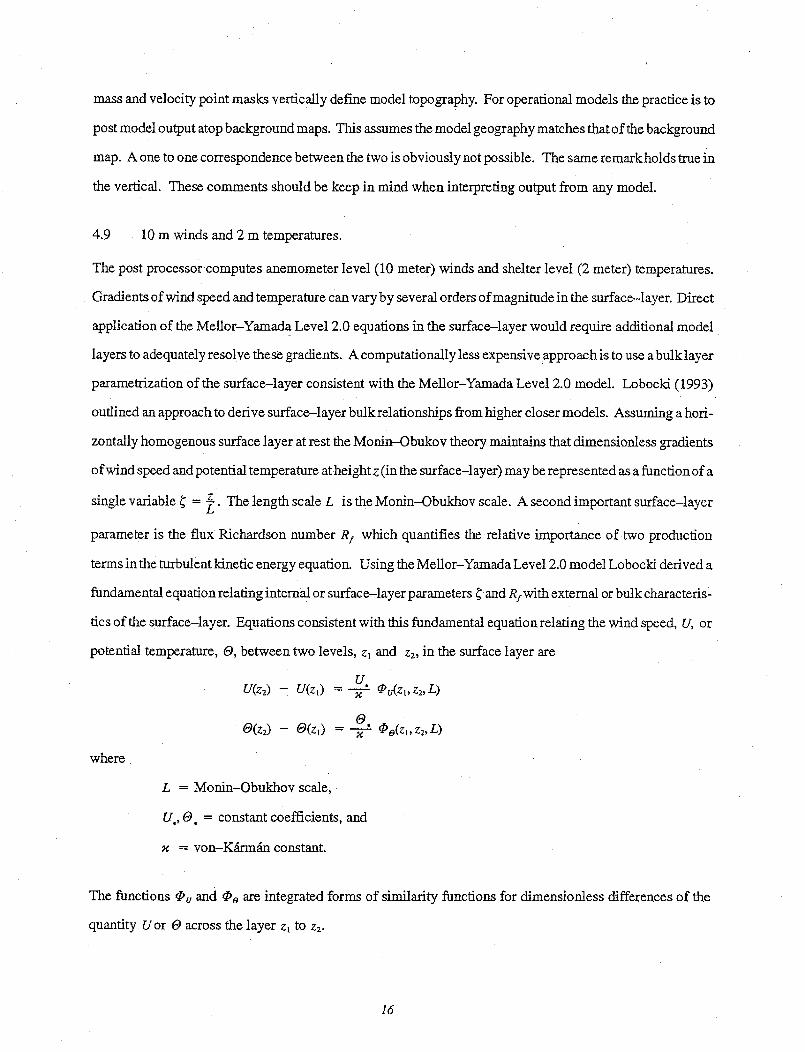
potential temperature, 9, between two levels, z1 and z2, in the surface layer are
UU(z 2) - U(Z1) = X 'U(Zl, Z12,L)
0(z2) - e(z 1) = X Po(zt ' Z2 , L)
where
L = Monin-Obukhov scale,
U., . = constant coefficients, and
x = von-KArm6n constant.
The functions Au and 'P are integrated forms of similarity functions for dimensionless differences of the
quantity U or e across the layer z, to z2.
16
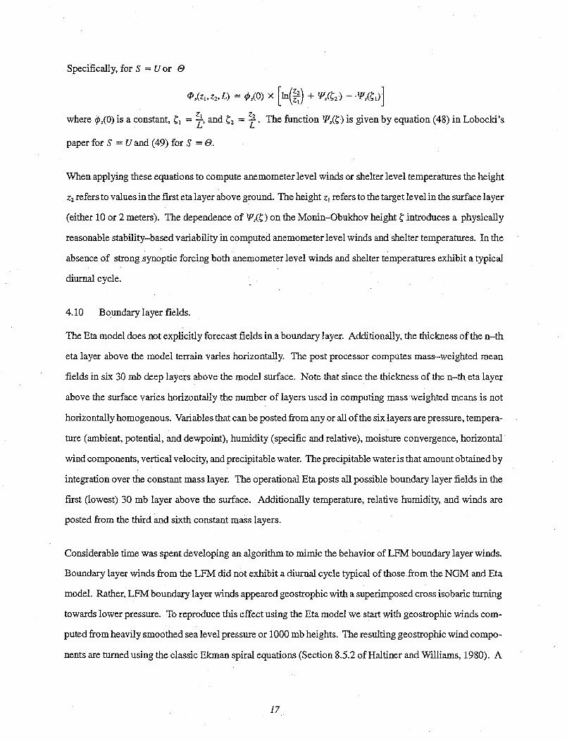
Specifically, for S = U or )
0,(zIz 2,L) = ,() x [n(Z) + P( 2) -
where 0(0) is a constant, z = Z and z2 = .- The function PF(. ) is given by equation (48) in Lobocki's
paper for S = U and (49) for S = 6.
When applying these equations to compute anemometer level winds or shelter level temperatures the height
z2 refers to values in the first eta layer above ground. The height z, refers to the target level in the surface layer
(either 10 or 2 meters). The dependence of W(.) on the Monin-Obukhov height ~ introduces a physically
reasonable stability-based variability in computed anemometer level winds and shelter temperatures. In the
absence of strong synoptic forcing both anemometer level winds and shelter temperatures exhibit a typical
diurnal cycle.
4.10 Boundary layer fields.
The Eta model does not explicitly forecast fields in a boundary layer. Additionally, the thickness of the n-th
eta layer above the model terrain varies horizontally. The post processor computes mass-weighted mean
fields in six 30 mb deep layers above the model surface. Note that since the thickness of the n-th eta layer
above the surface varies horizontally the number of layers used in computing mass weighted means is not
horizontally homogenous. Variables that can be posted from any or all of the six layers are pressure, tempera-
ture (ambient, potential, and dewpoint), humidity (specific and relative), moisture convergence, horizontal
wind components, vertical velocity, and precipitable water. The precipitable water is that amount obtained by
integration over the constant mass layer. The operational Eta posts all possible boundary layer fields in the
first (lowest) 30 mb layer above the surface. Additionally temperature, relative humidity, and winds are
posted from the third and sixth constant mass layers.
Considerable time was spent developing an algorithm to mimic the behavior of LFM boundary layer winds.
Boundary layer winds from the LFM did not exhibit a diurnal cycle typical of those from the NGM and Eta
model. Rather, LFM boundary layer winds appeared geostrophic with a superimposed cross isobaric turning
towards lower pressure. To reproduce this effect using the Eta model we start with geostrophic winds com-
puted from heavily smoothed sea level pressure or 1000 mb heights. The resulting geostrophic wind compo-
nents are turned using the classic Ekman spiral equations (Section 8.5.2 of Haltiner and Williams, 1980). A
17
rotation parameter controls the amount of the cross contour flow. After much experimentation a suitable rota-
tion parameter along with appropriate smoothing was found to produce a wind field very comparable to the
LFM boundary layer winds. This method is not currently used in the operational Eta.
4.11 LFM and NGM look-alike fields.
In addition to posting standard data on pressure surfaces or deriving other fields from model output, the post
processor generates fields specific to the LFM and NGM using Eta model output These fields are written to
the output file using LFM or NGM labels. The primary reason for including these look-alike fields was to
ensure compatibility of posted Eta model output with existing graphics and bulletin generating codes.
The post computes equivalents to fields in the NGM first (S1=0.98230), third (S3=0.89671), and fifth
(S5=0.78483) sigma layers data as well as layer mean relative humidities and a layer mean moisture conver-
gence field. Recall the definition of the sigma coordinate,
P -P tPs - Pt
Given the pressure at the top of the model (p, = 50mb) and the forecast surface pressure pi target sigmalevels
are converted to pressure equivalents. Vertical interpolationfromthe etalayers bounding each targetpressure
provides aneta-based approximation to the field onthe targetsigmalevel. This calculationis repeated at each
horizontal grid point to obtain eta-based sigma level S 1, S3, S5 temperatures, S 1 relative humidity, and S 1 u
and v wind components. Since surface pressure is carried at mass points a four point average of the winds
surrounding each mass pointis usedin computing the S 1 u and v wind components. A check is made to ensure
zero winds are not included in this average. S3 and S5 relative humidities are layer means over the eta layers
mapping into sigma layers 0.47 to 0.96 and 0.18 to 0.47, respectively.
The FOUS 60-78 NWS bulletins are generated from the NGM look-alike fields and other posted fields.
These bulletins contain initial condition and six hourly forecasts out to forecast hour 48 for thirteen parame-
ters at sites over the U.S., Canada, and coastal waters. Table 1 identifies which Eta fields are used in generat-
ing these bulletins.
LFM look-alike fields include three layer mean relative humidities and a partial column precipitable water.
An approach similar to that used for the NGM is not directly applicable. The distinction arises due to the
vertical structure of the LFM. The approach taken here was to assume a sigma based vertical coordinate in the
18
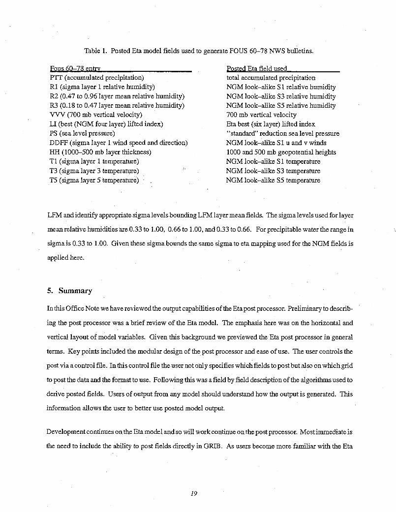
Table 1. Posted Eta model fields used to generate FOUS 60-78 NWS bulletins.
Fous 60-78 entrvPTT (accumulated precipitation)R1 (sigma layer 1 relative humidity)R2 (0.47 to 0.96 layer mean relative humidity)R3 (0.18 to 0.47 layer mean relative humidity)VVV (700 mb vertical velocity)LI (best (NGM four layer) lifted index)PS (sea level pressure)DDFF (sigma layer 1 wind speed and direction)HH (1000-500 mb layer thickness)T1 (sigma layer 1 temperature)T3 (sigma layer 3 temperature)
T5 (sigma layer 5 temperature)
Posted Eta field usedtotal accumulated precipitationNGM look-alike S 1 relative humidityNGM look-alike S3 relative humidityNGM look-alike S5 relative humidity700 mb vertical velocity
Eta best (six layer) lifted index"standard" reduction sea level pressureNGM look-alike S 1 u and v winds1000 and 500 mb geopotential heights
NGM look-alike S 1 temperatureNGM look-alike S3 temperatureNGM look-alike S5 temperature
LFM and identify appropriate sigma levels bounding LFM layer mean fields. The sigma levels used for layer
mean relative humidities are 0.33 to 1.00, 0.66 to 1.00, and 0.33 to 0.66. For precipitable water the range in
sigma is 0.33 to 1.00. Given these sigma bounds the same sigma to eta mapping used for the NGM fields is
applied here.
5. Summary
In this Office Note we have reviewed the output capabilities of the Eta post processor. Preliminary to describ-
ing the post processor was a brief review of the Eta model. The emphasis here was on the horizontal and
vertical layout of model variables. Given this background we previewed the Eta post processor in general
terms. Key points included the modular design of the post processor and ease of use. The user controls the
post via acontrol file. Inthis control file theusernot only specifies whichfields to postbut also onwhichgrid
to post the data and the format to use. Following this was a field by field description of the algorithms used to
derive posted fields. Users of output from any model should understand how the output is generated. This
information allows the user to better use posted model output.
Development continues on the Eta model and so will work continue on the postprocessor. Mostimmediate is
the need to include the ability to post fields directly in GRIB. As users become more familiar with the Eta
19
model it is envisioned their feedback will suggest the addition or deletion of routines. Such communication
can play an important but often overlooked role in development.
6. References
Atldkinson, B.W., 1981: Meso-scale Atmospheric Circulations, Academic Press, New York, 495 pp.
Betts, A.K., 1986: A new convective adjustment scheme. PartI: observational and theoretical basis. Quart.J. Roy. Meteor. Soc., 112, 677-691.
-, and M.J. Miller,1986: A new convective adjustment scheme. Part II: single column tests using GATEwave, BOMEX, and artic air-mass data sets. Quart J. Roy. Meteor. Soc., 112, 693-709.
Black, T., 1988: The step mountain, eta coordinate model: A documentation. NMC/NWS Washington, 47pp [Available from NMC, 5200 Auth Road, Washington, D.C. 20233].
-,1993: The step-mountainetacoordinate mesoscale model attheNational Meteorological Center, inprep-aration.
Bolton, D., 1980: The computation of equivalent potential temperature. Mon. Wea. Rev., 108, 1046-1053.
Campana, K.A., and P.M. Caplan, 1989: Diagnosed cloud specifications, Research Highlights of the NMCDevelopment Division: 1987-1988, 101-111.
-,P.M. Caplan, G.H. White, S.K. Yang, and H.M. Juang, 1990: Impact of changes to cloud parameterizationon the forecast error of NMC's global model, Preprints Seventh Conference on Atmospheric Radiation,San Francisco, CA, Amer. Meteor. Soc., J152-J158.
Carpenter, R.L., Jr., K.K. Droegemeier, P.W. Woodward, and C.E. Hane, 1989: Application of the piecewiseparabolic method (PPM) to meteorological modeling. Mon. Wea. Rev., 118, 586-612.
Cotton, W.R., and R.A. Anthes, 1989: Storm and Cloud Dynamics, Academic Press, New York, 880 pp.
Cram, J.M., and R.A. Pielke, 1989: A further comparison of two synoptic surface wind and pressure analysismethods. Mon. Wea. Rev., 117, 696-706.
Deardorff, J., 1978: Efficient prediction of ground temperature and moisture with inclusion of a layer of ve-getation. J. Geophys. Res., 83, 1989-1903.
Haltiner, G.J., and R.T. Williams, 1980: Numerical Prediction and Dynamic Meteorology. John Wilely &Sons, New York, 477 pp.
Janjic , Z.I., 1974: A stable centered difference scheme free of two-grid-interval noise. Mon. Wea. Rev., 102,319-323.
-,1979: Forward-backward scheme modified to prevent two-grid-interval noise and its application in sig-ma coordinate models. Contrib. Atmos. Phys., 52, 69-84.
-,1984: Nonlinear advection schemes and energy cascade on semistaggered grids. Mon. Wea. Rev., 112,1234-1245.
-, 1990: The step-mountain coordinate: physical package. Mon. Wea. Rev., 118, 1429-1443.
Keyser, D.A., 1990: NMC Development Divsion Rotating Random Access DiskArchive - UserDocumenta-tion. [Available from NMC, 5200 Auth Road, Washington, D.C., 20233].
Lobocki, L., 1993: A procedure for the derivation of surface-layer bulk relationships from simplified se-cond-order closure models. J. Appl. Meteor., 32, 126-138.
Mellor, G.L., and T. Yamada, 1974: A hierarchy of turbulence closure models for planetary boundary layers.JAtmos. Sci., 31, 1791-1806.
20
-, and-, 1982: Development of a turbulence closure model for geophysical fluid problems. Rev. Geophys.Space Phys., 20, 851-875.
Mesinger, F., 1973: A method for construction of second-order accuracy difference schemes permitting nofalse two-grid-interval wave in the height field. Tellus, 25, 444 458.
-, 1974: An economical explicit scheme which inherently prevents the false two-grid-interval wave inforecast fields. Proc. Symp. on Difference and Spectral MethodsforAtmosphere and Ocean DynamicsProblems, Novosibirsk, Acad. Sci., Novosibirsk, Part II, 18-34.
-,1984: A blocking technique for representation of mountains in atmospheric models. Riv. Meteor. Aero-nautica, 44, 195-202.
-,1990: Horizontal pressure reduction to sea level. Proc. 21st Conf for Alpine Meteor, Zurich, Switzer-land, 31-35.
Miyakoda, K., and J. Sirutis, 1983: Impact of sub-grid scale parameterizations on monthly forecasts. Proc.ECMWF Workshop on Convection in Large-Scale Models, ECMWF, Reading, England, 231-277.
Phillips, N.A., 1957: A coordinate system having some special advantages for numerical forecasting. J. Me-teor., 14, 297-300.
Saucier W.J., 1957: Principles of Meteorological Analysis, Dover Publications, New York, 438 pp.
Slingo, J.M., 1980: A cloud parameterization scheme derived from GATE data for use with a numerical mod-el. Quart J. Roy. Met. Soc., 106, 747-770.
Smagorinsky, J.J., L. Holloway, Jr., and G.D. Hembree, 1967: Prediction experiments with a general circula-tion model, Proc. Inter. Symp. DynamicsLarge ScaleAtmospheric Processes. Nauka, Moscow, U.S.S.R.,70-134.
Stackpole, J., 1990: NMC Handbook [Available from NMC, 5200 Auth Road, Washington, D.C., 20233].
Zhang, G.J., and N.A. McFarlane, 1991: Convective Stabilization in Midlatitudes. Mon. Wea. Rev., 119,1915-1928.
Ziltinkevitch, S.S., 1970: Dynamics of the planetary boundary layer. Gidrometeorologicheskoe Izdatelystvo,Leningrad, 292 pp. (in Russian).
21

Appendix 1: Fields Posted from the Operational Eta
7.1 Discussion
With the introduction of any new forecast model it is important to document what is available, where it is, and
in what format it is stored. This appendix attempts to fill this void by listing several sources of operational Eta
output. It does not address questions of accessing or unpacking the data. The last section lists LFM products
replaced by Eta products as of June 1993.
The operational Eta runs twice daily out to forecast hour 48. Fields are posted every six hours starting from
the initial conditions. The post processor generates two sets of sequential access Office Note 84 packed out-
put files, "FM" and "XP" files. To facilitate dissemination of Eta model output to the field across existing
communication circuits it was necessary to post Eta model output on the LFM forecast grid (Office Note 84
grid 26). These files are the FM files. Note that grid 26 has a mesh length of 190 km while the Eta model runs
on an approximately 80 km mesh. Obviously, significant detail can sometimes be lost in this interpolation.
To make the FM files completely compatible with preexisting codes a few additional fields posted to grids
other than grid 26 are appended to the FM files.
The XP files contain data posted to Office Note 84 grid 104, the NGM "super-C" grid. The horizontal resolu-
tion of this grid is approximately 90 km, comparable to that of the operational Eta. Precipitation forecasts on
the Eta model grid (90) are appended to this file. The XP files contain the most complete posting of Eta model
output. Their design and naming ("XP") was chosen to mimic similar files generated by the RAFS. FM files
contain a subset of the data posted to XP files.
The LFM posted an analysis to Office Note 84 grid 5 at the start of its integration. This analysis was a true
analysis and not the initial conditions used to start the LFM. The operational Eta posts its initial conditions to
grid 5 as well as to the FM and XP files. When the eta-based assimilation system is made operational a true
analysis may be posted to grid 5 if deemed necessary.
Operational Eta model output is archived in two databases. Permanent archiving of model output began with
the June 1993 implementation. The permanent database is the NMC Run History Tapes. The sequential ac-
cess, Office Note 84 packed XP and FM files are written to these tapes every cycle. Documentation for this
database is found in the NMC Handbook (Stackpole, 1990).
22

A second database for Eta forecasts is a rotating archive maintained by Development Division, NMC. The
XP files are written to a 36 day rotating ETAX archive. Not all fields posted to the XP file are written to the
ETAX archive. Further, data along the edges of grid 104 is stripped off leaving the smaller subgrid 105 which
is then archived. The FM files are written to a 7 day rotating archive named ETLX. Here data is archived on
grid 26. Not all fields posted to the FM files are written to this archive. Table 3 lists which fields are available
on the ETAX and ETLX archives. Documentation describing the rotating archive is "NMC Development
Division Rotating Random Access Archive: User Documentation" (Keyser 1990).
On a daily basis Eta model output is available in four forms: sequential Office Note 84 holding files, Office
Note 84 VSAM files, GRIB 1 formatted files, and PC-Grids files. These files reside on the NAS 9000 oper-
ated by the Department of Commerce at the Suitland Federal Center. Table 1 lists the names of these files on
the NAS 9000. The sequential access, Office Note 84 holding files are simply the XP and FM files generated
by the post processor. NAS 9000 jobs create VSAM files from these sequential files. Other than the file
format the VSAM and holding file versions of the XP and FM files are identical. Until GRIB is added to the
post processor, NAS 9000 codes generate GRIB 1 files from the sequential XP and FM files. The GRIB 1 XP
files contain data over the smaller grid 105. All fields on the XP and FM files are converted to GRIB 1. The
last format for posted Eta forecasts is PC-Grids. In this reformatting process grid 104 data is reduced to grid
105. Not all fields posted to the XP and FM files are written to PC-Grids files. Table 4 lists which fields are
posted to PC-Grids files. Note that the exact contents of the PC-Grids files will likely change in response to
future user requests.
Table 5 lists the first four hexadecimal words of the Office Note 84 label with which operational Eta fields are
packed. Admittedly, this table is of little use to users of the GRIB 1 or PC-Grids Eta files. However, since all
forms of Eta model output start from the Office Note 84 packed data sets it was decided to include these labels
in this Office Note. They definitively tell any user of the Office Note 84 packed Eta data sets what each field
is.
The last table (6) lists products generated from the operational Eta as of June 1993. Many of these replaced
LFM products. Others are unique to the Eta model. Note that Eta-based FOUS 60-78 NWS bulletins use the
NGM format and not that of the LFM. In the months following the June 1993 implementation additional Eta
based products will gradually come on line.
23

This concludes this brief overview of the availability and dissemination of operational Eta model output.
Following are several tables mentioned above. Please note that the specific contents of these listings are sub-
ject to change as the Eta model implementation progresses.
7.2 Table 1. Where is it?
Where can one find all this data? The above mentioned data sets reside on the NAS 9000 operated by the
Department of Commerce at the Suitland Federal Complex. The table below lists the filenames of these data-
sets.
File typeOffice Note 84 sequential analysisOffice Note 84 sequential XPOffice Note 84 sequential FM
Office Note 84 VSAM XP
Office Note 84 VSAM FM
GRIB1 XPGRIB1 FM
PC-Grids XPPC-Grids FM
NAS 9000 dataset name
NMC.PROD.LFANL. HOLD.ETANMC.PROD.LFxxXP.HOLD.ETANMC.PROD.LFxx.HOLD.ETANMC .PROD.VLFxxXP.TccZ.ETA
NMC.PROD.VLFxx.TccZ.ETACOM.CED1 .LFxxXP.TccZ.ETA
COM.CED 1 .LFcxx.TccZ.ETA
USR.WD20.PCGRIDS.TccZ.ETXCUSR.WD20.PCGRIDS.TccZ.ETAX
xx is the forecast hour in six hourly increments from 00 through 48.cc is the forecast cycle, 00 or 12.
24
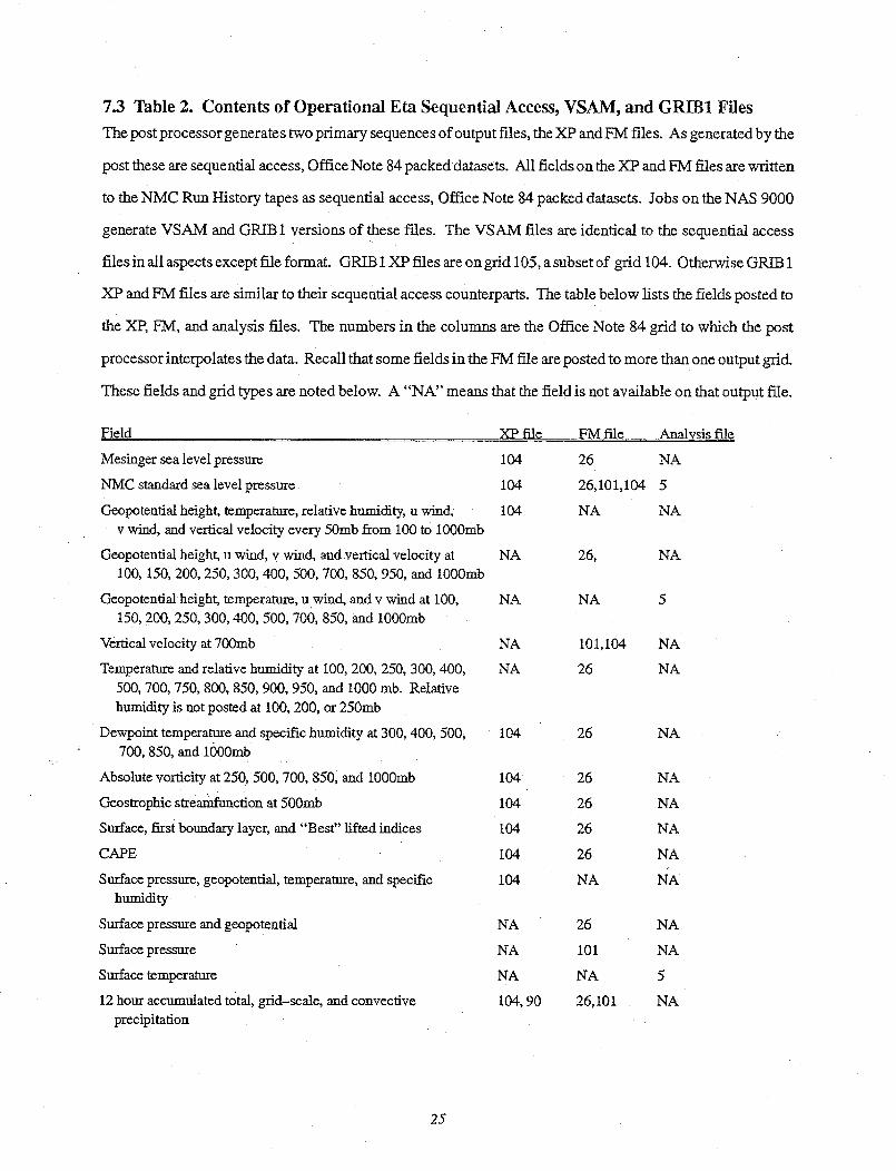
73 Table 2. Contents of Operational Eta Sequential Access, VSAM, and GRIB1 Files
The post processor generates two primary sequences of output files, the XP and FM files. As generated by the
post these are sequential access, Office Note 84 packed datasets. All fields on the XP and FM files are written
to the NMC Run History tapes as sequential access, Office Note 84 packed datasets. Jobs on the NAS 9000
generate VSAM and GRIB 1 versions of these files. The VSAM files are identical to the sequential access
files in all aspects except file format. GRIB 1 XP files are on grid 105, a subset of grid 104. Otherwise CGRIB 1
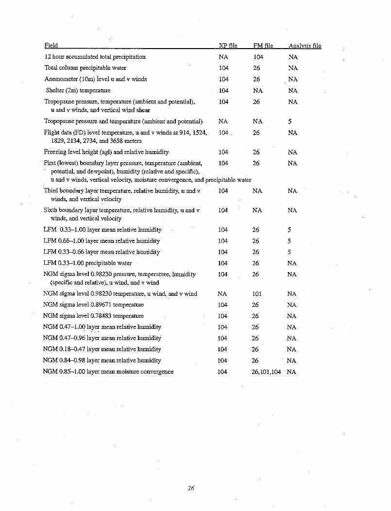
XP and FM files are similar to their sequential access counterparts. The table below lists the fields posted to
the XP, FM, and analysis files. The numbers in the columns are the Office Note 84 grid to which the post
processor interpolates the data. Recall that some fields in the FM file are posted to more than one output grid.
These fields and grid types are noted below. A "NA" means that the field is not available on that output file.
Field
Mesinger sea level pressure
NMC standard sea level pressure
Geopotential height, temperature, relative humidity, u wind,v wind, and vertical velocity every 50mb from 100 to 1000mb
Geopotential height, u wind, v wind, and vertical velocity at100, 150, 200,250,300,400, 500, 700, 850, 950, and 1000mb
Geopotenfial height, temperature, u wind, and v wind at 100,150, 200, 250, 300, 400, 500, 700, 850, and 1000mb
Vertical velocity at 700mb
Temperature and relative humidity at 100, 200, 250, 300, 400,
500, 700, 750, 800, 850, 900, 950, and 1000 mrb. Relative
humidity is not posted at 100, 200, or 250mb
Dewpoint temperature and specific humidity at 300, 400, 500,700, 850, and 1000mb
Absolute vorticity at 250, 500, 700, 850, and 1000mb
Geostrophic streanamfunction at 500mb
Surface, first boundary layer, and "Best" lifted indices
CAPE
Surface pressure, geopotential, temperature, and specifichumidity
Surface pressure and geopotential
Surface pressure
Surface temperature
12 hour accumulated total, grid-scale, and convectiveprecipitation
XP file
104
104
104
NA
FM file
26
26,101,104
NA
26,
NA NA
NA
NA
101,104
26
104 26
104
104
104
104
104
26
26
26
26
NA
NA
NA
NA
104, 90
26
101
NA
26,101
25
Analysis file
NA
5
NA
NA
5
NA
NA
NA
NA
NA
NA
NA
NA
NA
NA
NANA
XP file FM file Analysis file
12 hour accumulated total precipitation
Total column precipitable water
Anemometer (10m) level u and v winds
Shelter (2m) temperature
NA
104
104
104
Tropopause pressure, temperature (ambient and potential), 104u and v winds, and vertical wind shear
Tropopause pressure and temperature (ambient and potential) NA
Flight data (FD) level temperature, u and v winds at 914, 1524, 1041829, 2134, 2734, and 3658 meters
Freezing level height (agl) and relative humidity 104
First (lowest) boundary layer pressure, temperature (ambient, 104potential, and dewpoint), humidity (relative and specific),u and v winds, vertical velocity, moisture convergence, and precipitable water
Third boundary layer temperature, relative humidity, u and v 104winds, and vertical velocity
SLxth boundary layer temperature, relative humidity, u and v 104winds, and vertical velocity
LFM 0.33-1.00 layer mean relative humidity 104
LFM 0.66-1.00 layer mean relative humidity 104
LFM 0.33-0.66 layer mean relative humidity 104
LFM 0.33-1.00 precipitable water 104
NGM sigma level 0.98230 pressure, temperature, humidity 104(specific and relative), u wind, and v wind
NGM sigma level 0.98230 temperature, u wind, and v wind NA
NGM sigma level 0.89671 temperature 104
NGM sigma level 0.78483 temperature 104
NGM 0.47-1.00 layer mean relative humidity 104
NGM 0.47-0.96 layer mean relative humidity 104
NGM 0.18-0.47 layer mean relative humidity 104
NGM 0.84-0.98 layer mean relative humidity 104
NGM 0.85-1.00 layer mean moisture convergence 104
104
26
26
NA
26
NA
26
NA
NA
NA
NA
NA
5
NA
26
26
NA
NA
NA NA
NA NA
26
26
26
26
26
5
5
5
NA
NA
101 NA
26 NA
26 NA
26 NA
26 NA
26 NA
26 NA
26,101,104 NA
26
Field
7.4 Table 3. Contents of Operational Eta Rotating Archives
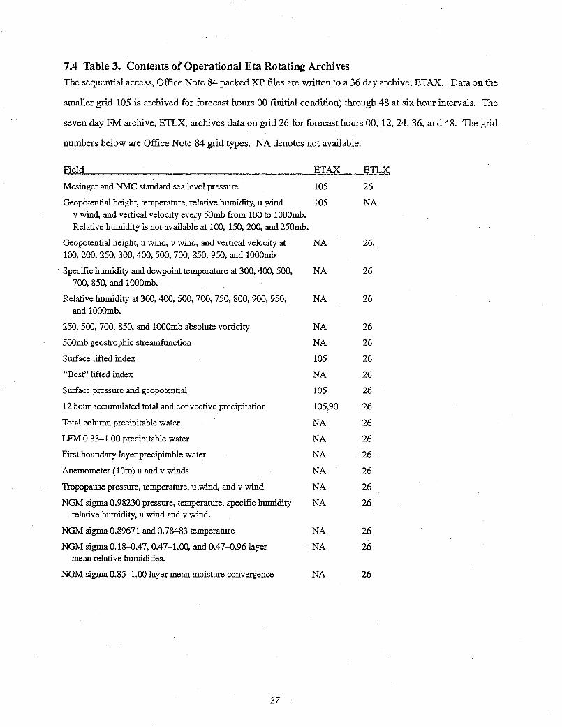
The sequential access, Office Note 84 packed XP files are written to a 36 day archive, ETAX. Data on the
smaller grid 105 is archived for forecast hours 00 (initial condition) through 48 at six hour intervals. The
seven day FM archive, ETLX, archives data on grid 26 for forecast hours 00, 12, 24, 36, and 48. The grid
numbers below are Office Note 84 grid types. NA denotes not available.
Field ETAX ETLX
Mesinger and NMC standard sea level pressure 105 26
Geopotential height, temperature, relative humidity, u wind 105 NAv wind, and vertical velocity every 50mb from 100 to 1000mb.Relative humidity is not available at 100, 150, 200, and 250mb.
Geopotential height, u wind, v wind, and vertical velocity at NA 26,100, 200, 250, 300, 400, 500, 700, 850, 950, and 1000mb
Specific humidity and dewpoint temperature at 300, 400, 500, NA 26700, 850, and 1000mb.
Relative humidity at 300, 400, 500, 700, 750, 800, 900, 950, NA 26and 1000mb.
250, 500, 700, 850, and 1000mb absolute vorticity NA 26
500mb geostrophic streamfunction NA 26
Surface lifted index 105 26
"Best" lifted index NA 26
Surface pressure and geopotential 105 26
12 hour accumulated total and convective precipitation 105,90 26
Total column precipitable water NA 26
LFM 0.33-1.00 precipitable water NA 26
First boundary layer precipitable water NA 26
Anemometer (10m) u and v winds NA 26
Tropopause pressure, temperature, u wind, and v wind NA 26
NGM sigma 0.98230 pressure, temperature, specific humidity NA 26relative humidity, u wind and v wind.
NGM sigma 0.89671 and 0.78483 temperature NA 26
NGM sigma 0.18-0.47, 0.47-1.00, and 0.47-0.96 layer NA 26mean relative humidities.
NGM sigma 0.85-1.00 layer mean moisture convergence NA 26
27

7.5 Table 4. Contents of Operational Eta PC-Grids FilesThe table below lists operational Eta fields available in PC-Grids format. The smaller grid 105 is extracted
from the XP files and converted to PC-Grids format. AVBL means the field is on the file; NA, not available.
Field
NMC standard sea level pressure
XP files FM files
AVBL AVBL
Geopotential height, temperature, u wind, v wind, and vertical AVBLvelocity at 100, 150, 200, 250, 300, 400, 500, 700, 850, and
1000mb. The FM PC-Grids file does not contain 100 or 150mb data.
500mb absolute vorticity NA
Relative humidity at 300, 400, 500, 700, 850, and 1000mb AVBL
Specific humidity at 300, 400, 500, 700, 850, and 1000mb NA
Surface pressure and geopotential AVBLThe FM PC-Grids file only contains surface pressure.
Surface lifted index AVBL
12 hour accumulated total and convective precipitation
Total column precipitable water
Anemometer (1 Om) winds
First boundary layer pressure, temperature, relativehumidity, u wind, and v wind.
AVBL
AVBL
NA
AVBL
28
AVBL
AVBL
NA
AVBL
AVBL
AVBL
AVBL
AVBL
AVBL
AVBL

7.6 Table 5. Office Note 84 Labels of Posted Eta Fields
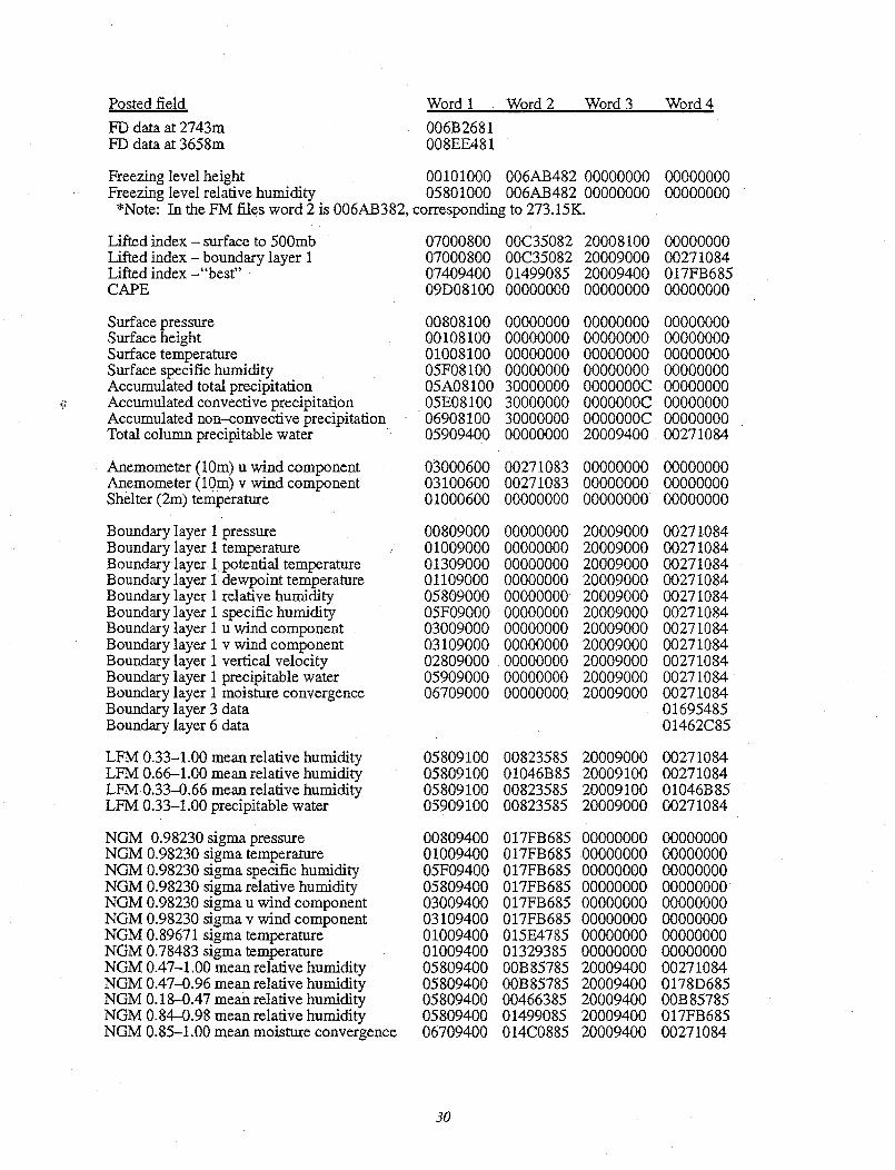
The table below lists all the fields posted from the operational Eta along with the first four hexadecimal words
of the Office Note 84 label with which each field is packed. We assume the reader is familiar with the Office
Note 84 packing convention. The listing below is for 00 hour posted fields. The same fields are written every
six hours.
Posted field
Mesinger sea level pressureNMC standard sea level pressure
500mb geopotential height500mb temperature500mb dewpoint temperature500mb relative humidity500mb specific humidity500mb u wind component500mb v wind component500mb vertical velocity500mb absolute vorticity500mb geostrophic streamfunction
100mb data150mb data200mb data250mb data300mb data350mb data400mb data450mb data550mb data600mb data650mb data700mb data750mb data800mb data850mb data900mb data950mb data1000mb data
Tropopause pressureTropopause temperatureTropopause u wind componentTropopause v wind componentTropopause vertical wind shear
FD temperature at 914mFD u wind component at 914mFD v wind component at 914mFD data at 1524mFD data at 1829mFD data at 2143m
Word 1 Word 2
00808A00 0000000000808000 00000000
0010080001000800011008000580080005F008000300080003100800028008000480080005000800
0080820001008200030082000310820003408200
010001000300010003100100
Word 3 Word4
00000000 0000000000000000 00000000
00C35082 0000000000C35082 0000000000C35082 0000000000C35082 0000000000C35082 0000000000C35082 0000000000C35082 0000000000C35082 0000000000C35082 0000000000C35082 00000000
00271082003A9882004E20820061A882007530820088B882009C408200AFC88200D6D88200EA608200FDE882011170820124F88201388082014C0882015F90820173188200271081
0000000000000000000000000000000000000000
016508820165088201650882003B88810047728100535C81
0000000000000000000000000000000000000000
000000000000000000000000
29
00000000000000000000000000000000000000000000000000000000000000000000000000000000
0000000000000000000000000000000000000000
000000000000000000000000
Word 2 Word 3 Word 4Posted field
FD data at 2743mFD data at 3658m
Freezing level height 00101000 006AB482 00000000Freezing level relative humidity 05801000 006AB482 00000000
*Note: In the FM files word 2 is 006AB382, corresponding to 273.15K.
Lifted index - surface to 500mbLifted index - boundary layer 1Lifted index -"best"CAPE
07000800070008000740940009D08100
Surface pressureSurface heightSurface temperatureSurface specific humidityAccumulated total precipitationAccumulated convective precipitationAccumulated non-convective precipitationTotal column precipitable water
Anemometer (10m) u wind componentAnemometer (10m) v wind componentShelter (2m) temperature
Boundary layer 1 pressureBoundary layer 1 temperatureBoundary layer 1 potential temperatureBoundary layer 1 dewpoint temperatureBoundary layer 1 relative humidityBoundary layer 1 specific humidityBoundary layer 1 u wind componentBoundary layer 1 v wind componentBoundary layer 1 vertical velocityBoundary layer 1 precipitable waterBoundary layer 1 moisture convergenceBoundary layer 3 dataBoundary layer 6 data
LFM 0.33-1.00 mean relative humidityLFM 0.66-1.00 mean relative humidityLFM 0.33-0.66 mean relative humidityLFM 0.33-1.00 precipitable water
NGM 0.98230 sigma pressureNGM 0.98230 sigma temperatureNGM 0.98230 sigma specific humidityNGM 0.98230 sigma relative humidityNGM 0.98230 sigma u wind componentNGM 0.98230 sigma v wind componentNGM 0.89671 sigma temperatureNGM 0.78483 sigma temperatureNGM 0.47-1.00 mean relative humidityNGM 0.47-0.96 mean relative humidityNGM 0.18-0.47 mean relative humidityNGM 0.84-0.98 mean relative humidityNGM 0.85-1.00 mean moisture convergence
00808100001081000100810005F0810005A0810005E081000690810005909400
030006000310060001000600
008090000100900001309000011090000580900005F090000300900003109000028090000590900006709000
05809100058091000580910005909100
008094000100940005F0940005809400030094000310940001009400010094000580940005809400058094000580940006709400
00C3508200C350820149908500000000
0000000000000000000000000000000030000000300000003000000000000000
002710830027108300000000
0000000000000000000000000000000000000000000000000000000000000000000000000000000000000000
0082358501046B850082358500823585
017FB685017FB685017FB685017FB685017FB685017FB685015E4785013293850OB 8578500B 857850046638501499085014C0885
20008100200090002000940000000000
0000000000000000
0000000000271084017FB68500000000
00000000 0000000000000000 0000000000000000 0000000000000000 00000000000000OC 00000000000000OC 00000000OOOOOOOC 0000000020009400 00271084
00000000 0000000000000000 0000000000000000 00000000
2000900020009000200090002000900020009000200090002000900020009000200090002000900020009000
20009000200091002000910020009000
00000000000000000000000000000000000000000000000000000000000000002000940020009400200094002000940020009400
00271084002710840027108400271084002710840027108400271084002710840027108400271084002710840169548501462C85
002710840027108401046B8500271084
0000000000000000000000000000000000000000000000000000000000000000002710840178D68500B 85785017FB68500271084
30
006B2681008EE481
Wnrd 1
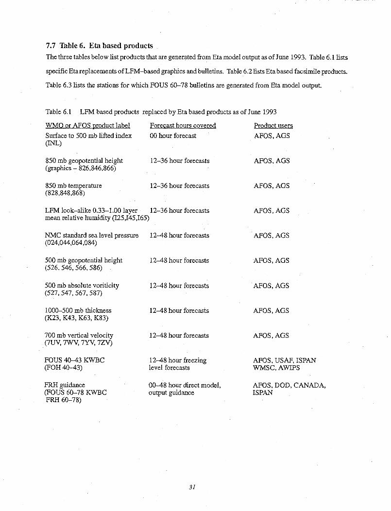
7.7 Table 6. Eta based productsThe three tables below list products that are generated from Eta model output as of June 1993. Table 6.1 lists
specific Etareplacements of LFM-based graphics and bulletins. Table 6.2 lists Eta based facsimile products.
Table 6.3 lists the stations for which FOUS 60-78 bulletins are generated from Eta model output.
Table 6.1 LFM based products replaced by Eta based products as of June 1993
WMO or AFOS product label Forecast hours covered Product users
Surface to 500 mb lifted index 00 hour forecast AFOS, AGS(INL)
850 mb geopotential height 12-36 hour forecasts AFOS, AGS(graphics - 826,846,866)
850 mb temperature 12-36 hour forecasts AFOS, AGS(828,848,868)
LFM look-alike 0.33-1.00 layer 12-36 hour forecasts AFOS, AGSmean relative humidity (I25,I45,I65)
NMC standard sea level pressure 12-48 hour forecasts AFOS, AGS(024,044,064,084)
500 mb geopotential height 12-48 hour forecasts AFOS, AGS(526, 546,566,586)
500 mb absolute voriticity 12-48 hour forecasts AFOS, AGS(527, 547,567, 587)
1000-500 mb thickness 12-48 hour forecasts AFOS, AGS(K23, K43, K63, K83)
700 mb vertical velocity 12-48 hour forecasts AFOS, AGS(7UV, 7WV, 7YV, 7ZV)
FOUS 40-43 KWBC 12-48 hour freezing AFOS, USAF, ISPAN(FOH 40-43) level forecasts WMSC, AWIPS
FRH guidance 00-48 hour direct model, AFOS, DOD, CANADA,(FOUS 60-78 KWBC output guidance ISPANFRH 60-78)
31

Table 6.2 Eta based facsimile products.
San Juan facsimile circuit:
Slot number Product description
J038 12hr 700 mb height and relative humidity12hr total accumulated precipitation and 700 mb vertical velocity12hr 500 mb height and vorticity12hr mean sea level pressure and 1000-500 mb thickness
Slot number Product description
J039 24hr 700 mb height and relative humidity24hr total accumulated precipitation and 700 mb vertical velocity24hr 500 mb height and vorticity24hr mean sea level pressure and 1000-500 mb thickness
J040 36hr 700 mb height and relative humidity36hr total accumulated precipitation and 700 mb vertical velocity36hr 500 nib height and vorticity36hr mean sea level pressure and 1000-500 mb thickness
48hr 700 mb height and relative humidity48hr total accumulated precipitation and 700 mb vertical velocity48hr 500 mb height and vorticity48hr mean sea level pressure and 1000-500 mb thickness
Alaska facsimile circuit:
Slot number Product description
A070 12hr 500 mb height and vorticity24hr 500 mb height36hr 500 mb height and vorticity
Difax facsimile circuit:
Slot number
D024
D154
D034
D169
Product description
00hr 500 mb height and vorticity (00Z)12hr 500 mb height and vorticity24hr 500 mb height and vorticity36hr 500 mb height and vorticity
00hr 500 mb height and vorticity (12Z)12hr 500 mb height and vorticity24hr 500 mb height and vorticity36hr 500 mb height and vorticity
FDFAX LFM FAXPLOT (point plots of model winds and temperatures) (00Z)
FDFAX LFM FAXPLOT (12Z)
32
J044
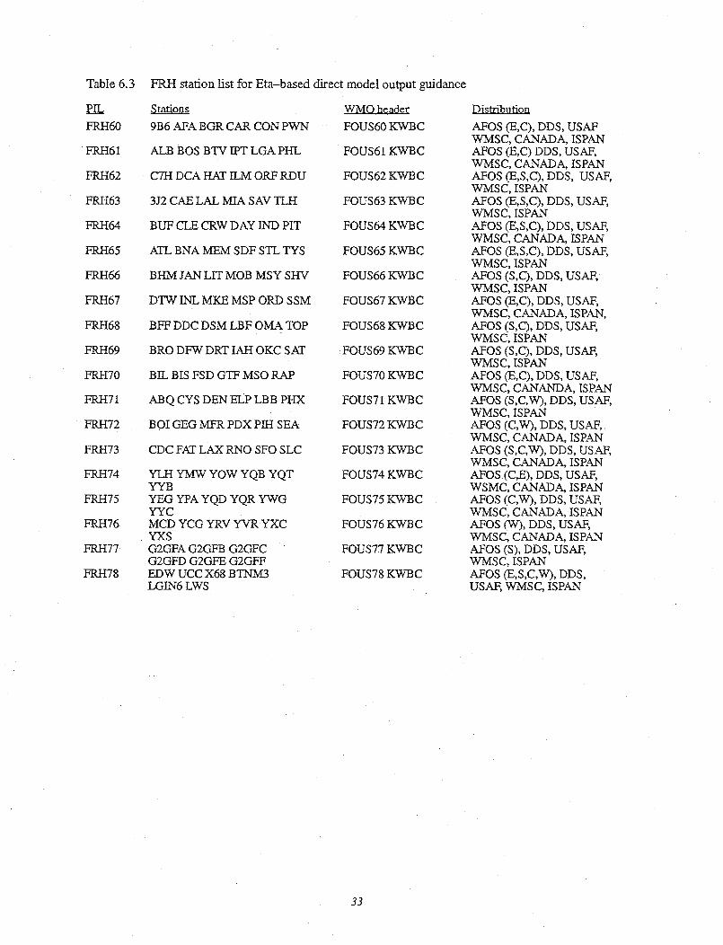
Table 6.3 FRH station list for Eta-based direct model output guidance
PIL StationsFRH60 9B6 AFA BGR CAR CON PWN
FRH61 ALB BOS BTVIPTLGAPHL
FRH62 C7H DCA HAT ILM ORF RDU
FRH63 3J2 CAE LAL MIA SAV TLH
FRH64 BUF CLE CRW DAY IND PIT
FRH65 ATL BNA MEM SDF STL TYS
FRH66 BHM JAN LIT MOB MSY SHV
FRH67 DTW INL MKE MSP ORD SSM
FRH68 BFF DDC DSM LBF OMA TOP
FRH69 BRO DFW DRT IAH OKC SAT
FRH70 BIL BIS FSD GTF MSO RAP
FRH71 ABQ CYS DEN ELP LBB PHX
FRH72 BOI GEG MFR PDX PIH SEA
FRH73 CDC FAT LAX RNO SFO SLC
FRH74 YLH YMW YOW YQB YQTYYB
FRH75 YEG YPA YQD YQR YWGYYC
FRH76 MCD YCG YRV YVR YXCYXS
FRH77 G2GFA G2GFB G2GFCG2GFD G2GFE G2GFF
FRH78 EDW UCC X68 BTNM3LGIN6 LWS
WMO header
FOUS60 KWBC
FOUS61 KWBC
FOUS62 KWBC
FOUS63 KWBC
FOUS64 KWBC
FOUS65 KWBC
FOUS66 KWBC
FOUS67 KWBC
FOUS68 KWBC
FOUS69 KWBC
FOUS70 KWBC
FOUS71 KWBC
FOUS72 KWBC
FOUS73 KWBC
FOUS74 KWBC
FOUS75 KWBC
FOUS76 KWBC
FOUS77 KWBC
FOUS78 KWBC
Distribution
AFOS (E,C), DDS, USAFWMSC, CANADA, ISPANAFOS (E,C) DDS, USAF,WMSC, CANADA, ISPANAFOS (E,S,C), DDS, USAF,WMSC, ISPANAFOS (E,S,C), DDS, USAF,WMSC, ISPANAFOS (E,S,C), DDS, USAF,WMSC, CANADA, ISPANAFOS (E,S,C), DDS, USAF,WMSC, ISPANAFOS (S,C), DDS, USAF,WMSC, ISPANAFOS (E,C), DDS, USAF,WMSC, CANADA, ISPAN,AFOS (S,C), DDS, USAF,WMSC, ISPANAFOS (S,C), DDS, USAF,WMSC, ISPANAFOS (E,C), DDS, USAF,WMSC, CANANDA, ISPANAFOS (S,C,W), DDS, USAF,WMSC, ISPANAFOS (C,W), DDS, USAF,WMSC, CANADA, ISPANAFOS (S,C,W), DDS, USAF,WMSC, CANADA, ISPANAFOS (C,E), DDS, USAF,WSMC, CANADA, ISPANAFOS (C,W), DDS, USAF,WMSC, CANADA, ISPANAFOS (W), DDS, USAF,WMSC, CANADA, ISPANAFOS (S), DDS, USAF,WMSC, ISPANAFOS (E,S,C,W), DDS,USAF, WMSC, ISPAN
33
Appendix 2: Using the Eta Post Processor
8.1 Introduction
In this appendix we discuss in greater detail how to use the Eta post processor. We assume the reader knows
how to run the Eta model. The peculiarities of any single user application necessarily limits how specific our
treatment can be. It is hoped enough information is given to get the reader started using the Eta post processor.
8.2 Namelist FCSTDATA
Prior to running the model the user must set variables in namelist FCSTDATA accordingly. We draw atten-
tion only to those variables in FCSTDATA which impact the post processor. These are TSTART, TEND,
TPREC, NMAP, TSHDE, and SPL. The model integration starts at hour TSTART and runs through hour
TEND. Total and convective precipitation are accumulated over periods TPREC hours long starting from
hour TSTART. The times (measured in hours) at which to post model fields are set in array TSHDE. NIMAP
is the number of posting times specified in array TSHDE. Currently the maximum number of posting times is
forty-nine. The only restriction on the output times is that they be between TSTART and TEND. Note that the
accumulation of precipitation over TPREC hour intervals operates independently of the posting times set in
TSHDE. The last variable of interest to the post processor in namelist FCSTDATAis array S PL. Through this
array the user sets the standard pressure levels (in Pascals) to which the post will be able to interpolate data.
We postpone discussion of how the pressures in S PL are interpreted by the post processor to the next section.
8.3 The Control File
The user interacts with the post processor through a control file. The set-up of this file is similar to one used
with the NGM. By editing the control file the user selects which fields to post, what grid to post the fields to,
and what format to output the fields in. If fields are to be posted to a grid other than the model grid interpola-
tion weights may be computed beforehand and read in. Depending on the number of output fields, calculation
of interpolation weights can require more CPU time than the time it takes to post the fields. Obviously, opera-
tional Eta runs utilize pre-computed interpolation weights. However, this is not necessary. The post retains
the ability to compute interpolation weights itself prior to posting fields. By stringing together several control
files the user may request that the same or different fields be posted on different output grids. In turn, these
different grids may be in the same or different output files.
34
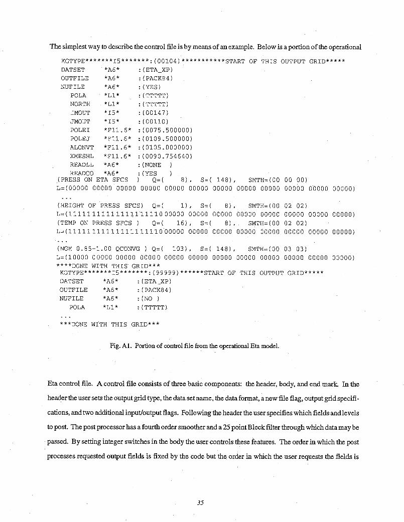
The simplest way to describe the control file is by means of an example. Below is a portion of the operational
KGTYPE*******I5*******:(00104)***********START OF THIS OUTPUT GRID*****DATSET *A6* :(ETA_XP)
OUTFILE *A6* :(PACK84)
NUFILE *A6* :(YES)
POLA *L1* :(TTTTT)
NORTH *L1* :(TTTTT)
IMOUT *I5* :(00147)
JMOUT *I5* :(00110)
POLEI *F11.6* :(0075.500000)POLEJ *F11.6* :(0109.500000)ALONVT *F11.6* :(0105.000000)XMESHL *F11.6* :(0090.754640)READLL *A6* :(NONE )READCO *A6* :(YES )
(PRESS ON ETA SFCS ) Q=( 8), S=( 148), SMTH=(00 00 00)
L=(00000 00000 00000 00000 00000 00000 00000 00000 00000 00000 00000 00000)
(HEIGHT OF PRESS SFCS) Q=( 1), S=( 8), SMTH=(00 02 02)L=(1111111111111111111000000 00000 00000 00000 00000 00000 00000 00000)
(TEMP ON PRESS SFCS ) Q=( 16), S=( 8), SMTH=(00 02 02)
L=(11111 11111 111111111000000 00000 00000 00000 00000 00000 00000 00000)
(NGM 0.85-1.00 QCONVG ) Q=( 103), S=( 148), SMTH=(00 03 03)
L=(10000 00000 00000 00000 00000 00000 00000 00000 00000 00000 00000 00000)****DONE WITH THIS GRID***KGTYPE*******I5*******:(99999)******START OF THIS OUTPUT GRID*****DATSET *A6* :(ETA_XP)
OUTFILE *A6* :(PACK84)
NUFILE *A6* :(NO )
POLA *L1* :(TTTTT)
***DONE WITH THIS GRID***
Fig. A1. Portion of control file from the operational Eta model.
Eta control file. A control file consists of three basic components: the header, body, and end mark. In the
header the user sets the output grid type, the data set name, the data format, a new file flag, output grid specifi-
cations, and two additional input/output flags. Following the header the user specifies which fields and levels
to post. The post processor has a fourth order smoother and a 25 point Bleck filter through which data may be
passed. By setting integer switches in the body the user controls these features. The order in which the post
processes requested output fields is fixed by the code but the order in which the user requests the fields is
35
immaterial. The body of a control file only needs to list those fields the user wants. To allow for this flexibil-
ity every control file must end with an end mark. The end mark line tells the post processor to stop reading the
control file and start posting requested fields.
At first glance the header block of a control file appears confusing. The key to understanding the header is
remembering what the variable name atthe start of eachline means. KGTYPE is a nonnegativeintegerrepre-
senting the type of output grid. The convention here is to use Office Note 84 grid types with two exceptions.
The first exception is shown at the bottom of Fig. Al. Grid type 9 9 9 9 9 is the staggered E grid, regardless of
the horizontal resolution. The second exception is grid type 0 0 0 0 0. This grid type instructs the code to post
the requested field(s) on a filled E grid. In the upper portion of Fig. Al grid type 104 is the NGM "super-C"
grid. The string "START OF THIS OUTPUT GRID" is simply added for readability. The post processor
ignores everything in the header outside of the parentheses. Each line of the header contains the data format
the post expects to read. Proper spacing is crucial. DATSET is the root from which the post generates output
filenames. To this root the post appends the forecast hour (e.,g., ETAXP0 0, ETA XP 6, etc.). Via the
character string OUTFILE the user specifies the format of the posted data. Currently two data formats are
available: unpacked (Cray) binary and Office Note 84. Setting DATSET to NOPACK tells the post to write
data using unformatted FORTRAN writes. A short program is available from the author to convert Cray
binary to other binary formats using the UNICOS assign statement. With DATS ET = PACK 8 4 an Office Note
84 packed data set is generated. At a later date the ability to post data directly in GRIB will be added. Current-
ly a program on the NAS 9000 converts Office Note 84 packed data sets to GRIB 1. Variable NUF I LE allows
the user to specify whether fields requested in the body are to be appended to a currently open output file or if a
new output file is to be opened. It is a simple YES or NO switch.
The indented variables in the header deal with the output grid and pre-computed interpolation weights.
POLA, NORTH, IMOUT, JMOUT, POLEI, POLEJ, ALONVT, and XMESHL are the basic set of
parameters by which standard NMC software defines polar stereographic grids. POLA and NORTH are log-
ical flags. Setting both to true (TTTTT) specifies a polar stereographic projection in the northern hemi-
sphere. (IMOUT, lMOUT) are the number of west-east and south-north grid points (directions relative to
the rotation specified by ALONVT). Grid point (1,1) is in the southwest corner of the grid; (IMOUT, JMOUT)
in the northeast corner. POLEI and POLEJ define the floating point (i,j) location of the pole point with
respect to the output grid. ALONVT is the longitude (west longitude being positive) from which grid east and
36

north are defined. Finally, XMESHL is the grid spacing in kilometers. Via these eight parameters all standard
polar stereographic NMC grids may be specified.
The user may sidestep this method to define an output grid by setting READLL to YES. This tells the post to
read an input file containing the geodetic latitude (glat) and longitude (glon) of output grid points. The
post canreadmultiple (glat,glon) files starting from unit number 30. The structure ofthe (glat,glon)
file expected by the post is (((glat(i,j),glon(i,j)),i=l,imout),j=l,jmout) using
FORMAT 5(gl 2.6, 1x). A word of caution. This option of the post has not been exhaustively tested
since most users desire data on standard polar stereographic NMC grids.
The last entry in the header block tells the post if pre-computed interpolation weights are available. Perfor-
mance timings showed that by far the largest percentage of CPU time executing the post was in computing
interpolation weights. If READCO is NONE the post computes all necessary interpolation weights once and
then proceeds with the posting. Having the post compute interpolation weights frees the user of this burden
and adds generality to the post. However, for repeated runs it is wise to compute the weights beforehand.
(Source is available from the author to compute these weights.) With READCO set to YES the post reads
weights starting from unit 20. If the control file has several output grids the unit number for the weights incre-
ments by one for each output grid up to a maximum unit number of 29. The user must ensure that the order in
which interpolation weights are assigned is the order in which the grids are listed in the control file (see Sec-
tion 8.4 for elaboration).
The bulk of the control file is the body. This is where the user specifies which fields to post and optionally the
degree of smoothing or filtering to apply to the posted fields. There arecurrently 110 unique fields that may be
posted from the Eta model. This, of course, is subject to change in response to model development and user
needs. As mentioned above it is not necessary to list all 110 available fields in the body of the control file.
Only those fields which are desired need to be listed. Each field specification consists of two lines. The first
line, the identifier line, starts with a brief description of the field. The post processor ignores this. Following
this are blocks Q= (xxx) and S= (xxx). The Q and S refer the first and second entries of the 27 element
Office Note 84 label. In any copy of the control file obtained from the author these labels are properly set.
The SMTH block on the identifier line controls the smoothing or filtering. In most applications the model to
output grid process involves two steps. First the staggered E grid is filled to make a regular grid. This is then
37
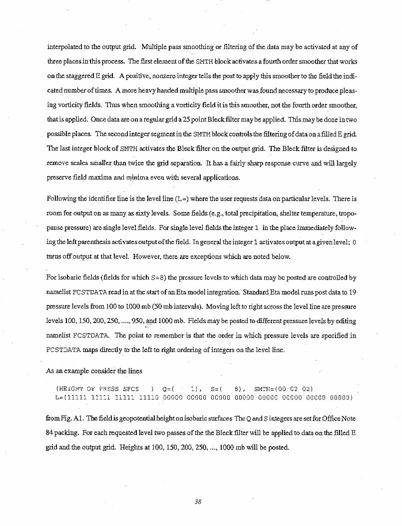
interpolated to the output grid. Multiple pass smoothing or filtering of the data may be activated at any of
three places in this process. The first element of the SMTH block activates a fourth order smoother that works
onthe staggered E grid. A positive, nonzero integer tells the post to apply this smoother to the field the indi-
cated number of times. A more heavy handed multiple pass smoother was found necessary to produce pleas-
ing vorticity fields. Thus when smoothing a vorticity field it is this smoother, not the fourth order smoother,
that is applied. Once data are on a regular grid a 25 point Bleck filter may be applied. This may be done in two
possible places. The second integer segment in the SMTH block controls the filtering of data on a filled E grid.
The last integer block of SMTH activates the Bleck filter on the output grid. The Bleck filter is designed to
remove scales smaller than twice the grid separation. It has a fairly sharp response curve and will largely
preserve field maxima and minima even with several applications.
Following the identifier line is the level line (L =) where the user requests data on particular levels. There is
room for output on as many as sixty levels. Some fields (e.g., total precipitation, shelter temperature, tropo-
pause pressure) are single level fields. For single level fields the integer 1 in the place immediately follow-
ing the left parenthesis activates output of the field. In general the integer 1 activates output at a given level; 0
turns off output at that level. However, there are exceptions which are noted below.
For isobaric fields (fields for which S= 8) the pressure levels to which data may be posted are controlled by
namelist FC STDATA read in at the start of an Eta model integration. Standard Eta model runs post data to 19
pressure levels from 100 to 1 000 mb (50 mb intervals). Moving left to right across the level line are pressure
levels 100, 150,200, 250 .... , 950, and 1000 mb. Fields may be posted to different pressure levels by editing
namelist FCSTDATA. The point to remember is that the order in which pressure levels are specified in
FCSTDATA maps directly to the left to right ordering of integers on the level line.
As an example consider the lines
(HEIGHT OF PRESS SFCS ) Q=( 1), S=( 8), SMTH=(00 02 02)
L=(11111 11111 11111 11110 00000 00000 00000 00000 00000 00000 00000 00000)
from Fig. Al. The fieldis geopotential height onisobaric surfaces The Q and S integers are set for Office Note
84 packing. For each requested level two passes of the the Bleck filter will be applied to data on the filled E
grid and the output grid. Heights at 100, 150, 200, 250, ..., 1000 mb will be posted.
38

For data on constant eta layers two options are available. Setting the n-th integer on the level line to 1
instructs the post to extract data on eta layer n. Note that the vertical numbering convention in the Eta model is
top down. That is, layer one is at the top of the model with the vertical index increasing downward. At times it
may be of interest to see what a selected field looks like in the n-th atmospheric eta layer. This is a terrain
following perspective. To activate this option set the n-th integer (left to right) on the level line to any integer
between 2 and 9, inclusive. For example, if a user wanted pressure data on the first, second, and fourth atmo-
spheric eta layers the specifications could look like
(PRESS ON ETA SFCS ) Q=( 8), S=( 148), SMTH=(00 00 00)L=(22020 00000 00000 00000 00000 00000 00000 00000 00000 00000 00000 00000)
In addition to eta layer and isobaric level data multiple levels may be requested for FD fields and boundary
layer fields. There are six FD levels. The ordering on the level line is from lowest to highestFD level. Bound-
ary layer fields are available from six 30 mb deep layers. The ordering on the level line is from the lowest
(nearest the surface) to the highest constant mass layer. All other fields are single level. That is, the leftmost
integer activates (1) or deactivates (0) posting of that field.
The last section of a control file is the end mark. This single line tells the post processor to stop reading the
control file and startpostingrequested fields. The key wordon theline is DONE. The post scans eachline read
from the control file for this string. It is the only way to specify the end of a control file.
As shown in Fig. A1 individual header-body-end control files may be chained together to output data in nu-
merous ways. The post reads the control files sequentially. If pre-computed interpolation weights are to be
read in the user must ensure that their assigned unit numbers correspond to the order in which the grids appear
in the combined control file. One last detail involves the end mark at the end of the last control file. The post
knows it has processed everything when it reads an end of file mark (EOF) from the control file. This EOF
must immediately follow the last DONE statement. If not, the post will unsuccessfully try to process what it
thinks is the next set of control cards.
8.4 The Template
If the post is to be run externally from the model the user must provide the model a "blank" template. The
template is a script which sets the stage for running the post, runs the post, and then cleans up after running the
post. The model reads and edits this template during the integration at posting times specified by the user
39
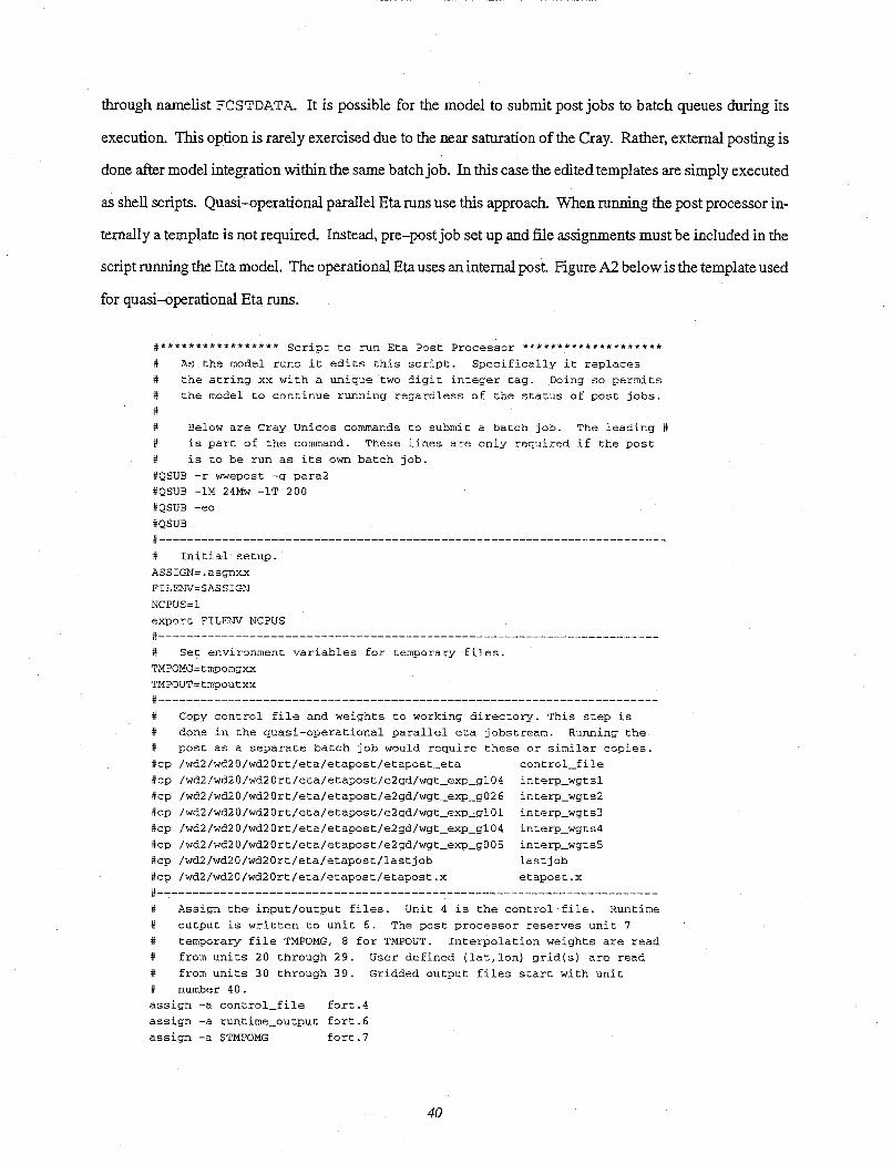
through namelist FCSTDATA. It is possible for the model to submit post jobs to batch queues during its
execution. This option is rarely exercised due to the near saturation of the Cray. Rather, external posting is
done after model integration within the same batch job. In this case the edited templates are simply executed
as shell scripts. Quasi-operational parallel Eta runs use this approach. When running the post processor in-
ternally a template is not required. Instead, pre-post job set up and file assignments must be included in the
script running the Eta model. The operational Eta uses an internal post. Figure A2 below is the template used
for quasi-operational Eta runs.
#***************** Script to run Eta Post Processor ******************
As the model runs it edits this script. Specifically it replaces
# the string xx with a unique two digit integer tag. Doing so permits
# the model to continue running regardless of the status of post jobs.
#Below are Cray Unicos commands to submit a batch job. The leading #
# is part of the command. These lines are only required if the post
# is to be run as its own batch job.
#QSUB -r wwepost -q para2
#QSUB -1M 24Mw -lT 200
#QSUB -eo
#QSUB
…# ...................- ------ _____________________.
# Initial setup.
ASSIC-N=.asgnxx
FILENV=$ASSIGN
NCPUS=l
export FILENV NCPUSif…#.................----…- _______- _____..._______
i Set environment variables for temporary files.
TMPOMG=tmpomgxx
TMPOUT=tmpoutxx
# if… . ............................................
# Copy control file and weights to working directory. This step is
done in the quasi-operational parallel eta jobstream. Running the
# post as a separate batch job would require these or similar copies.
#cp /wd2/wd20/wd20rt/eta/etapost/etapost_eta control_file
#cp /wd2/wd20/wd20rt/eta/etapost/e2gd/wgt_exp_g!04 interp_wgtsl
#cp /wd2/wd20/wd20rt/eta/etapost/e2gd/wgtexpg026 interp__wgts2
#cp /wd2/wd20/wd20rt/eta/etapost/e2gd/wgtexp_glOl interp_wgts3
#cp /wd2/wd20/wd20rt/eta/etapost/e2gd/wgtexpgl04 interpwgts4
#cp /wd2/wd20/wd20rt/eta/etapost/e2gd/wgtexpg005 interp_wgts5
#cp /wd2/wd20/wd20rt/eta/etapost/lastjob lastjob
#cp /wd2/wd20/wd20rt/eta/etapost/etapost.x etapost.x
if…#.................--- ____…- ___- _ _....._________
Assign the input/output files. Unit 4 is the control file. Runtime
# output is written to unit 6. The post processor reserves unit 7
# temporary file TMPOMG, 8 for TMPOUT. Interpolation weights are read
# from units 20 through 29. User defined (lat,lon) grid(s) are read
from units 30 through 39. Gridded output files start with unit
number 40.
assign -a control_file fort.4
assign -a runtime_output fort.6
assign -a $TMPOMG fort.7
40

assign -a $TMPOUT fort.8
assign -a interpwgtsl fort.20
assign -a interp_wgts2 fort.21
assign -a interp_wgts3 fort.22
assign -a interp_wgts4 fort.23
assign -a interpwgts5 fort.24......................................---------- ____________________...
Run the post processor.
etapost.x........................................................................
# Clean up after the posting job.
rm $TMPOMG $TMPOUT $ASSIGN core
#.- - - .- - - - _- -- - - - -- - - - -- - - - -- - - - - - -- - - -- - - -- - - - -- - - - -- - - -- - - - -- - -- - - - - --# If running the post as a batch job the user might want to trigger a
# sequence of jobs after the last set of fields are posted. This is
# not done for quasi-operational parallel Eta runs.
#LAST="sh lastjob"
#$LAST
#rm lastjob#- - - _ _ _ _ _ _ _ _ _ _ _ - -- - - - - - - - _ - - - _ _ _ _ _ _ _ _ - - - - - - - - _ _ _ _ _ - - -
End of output job.
exit
Fig. A2. Template for quasi-operational parallel Eta model runs.
8.5 Pre-computed Interpolation Weights
For many single or limited use applications it is not necessary or worthwhile to pre-compute interpolation
weights. The post will automatically compute these weights when the flag READCO=NONE. For repeated
model runs using the same model grid and output grids considerable time savings can be realized if pre-com-
puted weights are read in at the start of each post execution.
Source code is available from the author to pre-compute all necessary interpolation weights. All that is re-
quired are the Eta model grid specifications and those for the output grid or grids. These specifications are set
in namelists. For most grids the job to pre-compute interpolation weights can be run interactively on the
Cray.
8.6 Internal and External PostMention has already been made of the various modes in which the Eta post processor can be run; further elabo-
ration follows. In the early stages of development it was envisioned that the post processor would run as
stand-alone code external to the model. The model would spawn post jobs as it ran. The complexities of Cray
queuing priorities and scheduling, the near saturation of the Cray, and the time constraints of operational fore-
casting necessitated a version of the post that runs within the Eta model. Care has been taken to ensure consis-
41
tency between internal and external versions of the post processor. Virtually all aspects remain the same
between the two except for some subtle programming details.
In the internal mode pre-postjob steps and file assignments must be made in the script running the Eta model.
This removes the need for a template. Data required by the post is passed via commons. For the operational
Eta a batch job is spun off every twelve hours of model integration to dispose posted fields to the NAS 9000
for graphics generation and dissemination. The size of the combined model-post executable precludes its use
for non-operational model runs.
In the external mode the model edits a template at it runs. This template runs the post as discussed above.
Prior to editing the template the model dumps virtually all model variables in commons to temporary output
files named TMPOMGxx and TMPOUTxx. Creation of these temporary files allows the post to run externally
regardless of status of the model integration. Immediately upon termination of each post executable the used
temporary files are removed. The temporary files can be huge (TMPOUTxx is 60 Mb for the operational Eta
domain). The user should ensure that sufficient / tmp disk space is available under their user quota prior to
submitting the model run. For most applications this is not a problem.
Other than these brief remarks the variability from one user application to the next precludes a more detailed
discussion of how to set up the model and post. Sample scripts are available from the author which illustrate
various model-post configurations.
8.7 Summary
In this appendix we have described how to use the Eta post processor in conjunction with the model. The post
processor can be run either internal or external to the model. Most users will run the post externally after
model execution but within the same batch job. This necessitates a template which the model edits as it runs.
The user controls the post by editing a control file. In this file the user specifies the fields to post, smoothing,
data format, and output grids. This is common to all versions of the post. Both internal and external versions
of the post may read pre-computed interpolation weights.
Further details beyond those given getinto the specific needs of each user. Sample scripts and assistance are
available from the author.
42