1

Request to the National Oceanic and Atmospheric Administration for Incidental Take Regulations Governing Geophysical Surveys

on the Outer Continental Shelf of the Gulf of Mexico

(A response to Subpart I — MMPA Request Requirements at 50 CFR § 216.104)

Revision to original request package submitted December 20, 2002. Previous revisions provided in 2004, 2007, and 2011.

October 14, 2016

Submitted to: The Office of Protected Resources

1315 East-West Highway Silver Spring, Maryland 20910

Submitted by: Bureau of Ocean Energy Management

45600 Woodland Road Sterling, Virginia 20166

2

TABLE OF CONTENTS

Section 1 A Detailed Description of the Specific Activity or Class of Activities That Can Be Expected To Result in Incidental Taking of Marine Mammals ............................5

Section 2 The Date(s) and Duration of Such Activity and the Specific Geographical Region Where It Will Occur .....................................................................................35

Section 3 The Species and Numbers of Marine Mammals Likely To Be Found within the Activity Area; AND ..................................................................................................40

Section 4 A Description of the Status, Distribution, and Seasonal Distribution (When Applicable) of the Affected Species or Stocks of Marine Mammals Likely To Be Affected by Such Activities.................................................................................40

Section 5 The Type of Incidental Taking Authorization that Is Being Requested (i.e., Takes by Harassment Only or Takes by Harassment, Injury, and/or Death) and the Method of Incidental Taking ...............................................................................90

Section 6 By Age, Sex, and Reproductive Condition (If Possible), the Number of Marine Mammals (by Species) that May Be Taken by Each Type of Taking Identified in Paragraph (a)(5) of this Section, and the Number of Times Such Takings by Each Type of Taking Are Likely to Occur ...............................................................93

Section 7 Anticipated Impact of the Activity to the Species or Stock of Marine Mammal ...113

Section 8 The Anticipated Impact of the Activity on the Availability of the Species or Stocks of Marine Mammals for Subsistence Uses ..................................................133

Section 9 The Anticipated Impact of the Activity Upon the Habitat of the Marine Mammal Populations, and the Likelihood of Restoration of the Affected Habitat ................134

Section 10 The Anticipated Impact of the Loss or Modification of the Habitat on the Marine Mammal Populations Involved ..................................................................138

Section 11 The Availability and Feasibility (Economic and Technological) of Equipment, Methods, and Manner of Conducting Such Activity or Other Means of Affecting the Least Practicable Adverse Impact Upon the Affected Species or Stocks, Their Habitat, and on Their Availability for Subsistence Uses, Paying Particular Attention to Rookeries, Mating Grounds, and Areas of Similar Significance ........139

Section 12 Where the Proposed Activity Would Take Place In or Near a Traditional Arctic Subsistence Hunting Area and/or May Affect the Availability of a Species or Stock of Marine Mammal for Arctic Subsistence Uses, the Applicant Must Submit Either a Plan of Cooperation or Information That Identifies What

3

Measures Have Been Taken and/or Will Be Taken to Minimize Any Adverse Effects on the Availability of Marine Mammals for Subsistence Uses ..................151

Section 13 The Suggested Means of Accomplishing the Necessary Monitoring and Reporting that Will Result in Increased Knowledge of the Species, the Level of Taking or Impacts on Populations of Marine Mammals that Are Expected to Be Present while Conducting Activities and Suggested Means of Minimizing Burdens by Coordinating Such Reporting Requirements with Other Schemes Already Applicable to Persons Conducting Such Activity. Monitoring Plans Should Include a Description of the Survey Techniques that Would Be Used to Determine the Movement and Activity of Marine Mammals Near the Activity Site(S) Including Migration and Other Habitat Uses, Such as Feeding .................152

Section 14 Suggested Means of Learning of, Encouraging, and Coordinating Research Opportunities, Plans, and Activities Relating to Reducing Such Incidental Taking and Evaluating Its Effects ...........................................................................154

Section 15 References ...............................................................................................................157

Appendix A. JASCO Modeling Report ....................................................................................... A-1

5

1 A DETAILED DESCRIPTION OF THE SPECIFIC ACTIVITY OR CLASS OF ACTIVITIES THAT CAN BE EXPECTED TO RESULT IN INCIDENTAL TAKING OF MARINE MAMMALS

The Bureau of Ocean Energy Management (BOEM) is requesting regulations under Section (101)(5)(a) of the Marine Mammal Protection Act (MMPA) for the incidental take of marine mammals within the Outer Continental Shelf (OCS) of the Gulf of Mexico (GOM) associated with geophysical activities related to oil and gas exploration and development. BOEM is requesting these regulations for the geophysical contracting industries (hereinafter referred to as “industry” or “industries”) at the specific request of the National Marine Fisheries Service (NMFS). Should NMFS issue a regulation then subsequent Letters of Authorization (LOAs) will be applied for, in accordance with this regulation, by the aforementioned industries. Additionally, BOEM expects that subsequent requests for future regulations as needed in the GOM for geophysical activities related to oil and gas activities will be made by industry.

1.1 BACKGROUND On December 20, 2002, BOEM (formerly the Minerals Management Service [MMS])

petitioned NMFS for rulemaking under Section 101(a)(5)(A) of the MMPA to authorize any potential take of sperm whales (Physeter macrocephalus) incidental to conducting seismic surveys during oil and gas exploration activities in GOM. The petition for rulemaking was submitted at the request of NMFS so as to consolidate and more efficiently handle a larger number of activities within the specified geographic area. On March 3, 2003, NMFS published a notice of receipt of the petition and requested comments and information from the public (68 FR 9991), later extended to April 16, 2003 (68 FR 16262). BOEM prepared a Programmatic Environmental Assessment (PEA) for the petition, which was completed in July 2004. Based on the PEA findings, BOEM submitted a revised petition in September 2004 to request incidental take authorization for all NMFS-protected marine mammals considered to routinely inhabit the GOM and to be potentially impacted by oil and gas exploration and development activities. After several years of no action on the petition, pending the completion of a Programmatic Environmental Impact Statement (PEIS) by NMFS, BOEM provided NMFS with another revised MMPA petition on April 18, 2011, which incorporated updated information and analyses since the 2004 petition. The NMFS then followed with a Notice of Intent to prepare a PEIS on June 14, 2011 (76 FR 34656). On May 10, 2013, BOEM announced its intent to take over preparation of the PEIS and reopened a second public scoping period to gather public comments on the content and issues to consider in the PEIS (78 FR 27427). The Draft PEIS is currently available to the public for review. Given the time that has passed, BOEM is submitting another revision to the petition so as to incorporate the best available information that has developed since submission of its 2011 revised petition.

1.2 GEOPHYSICAL SURVEY TYPES A variety of geophysical techniques are used to characterize the shallow and deep structure

of the shelf, slope, and deepwater ocean environments. Geophysical surveys are conducted to (1) obtain data for hydrocarbon and mineral exploration and production; (2) aid in siting of oil and gas structures, facilities, and pipelines; (3) identify possible seafloor or shallow depth

6

geologic hazards; and (4) locate potential archaeological resources and benthic habitats that should be avoided. Geophysical surveys are performed to obtain indirect information on marine seabed and subsurface geology. High-resolution seismic surveys are designed to highlight seabed and near-surface potential obstructions, archaeology, and geohazards that may have safety implications during rig installation or well and development facility siting. Deep-focused seismic, electromagnetic, gravity, and magnetic surveys are designed to illuminate deeper subsurface structures and formations that may be of economic interest as a reservoir for oil and gas exploitation.

Geophysical activities are needed for operators to make business decisions about acquiring leases and maintaining reservoirs on leases. In addition to the needs of private industry, geophysical surveys provide important information for Government decisions. For example, BOEM uses deep two-dimensional (2D) and three-dimensional (3D) seismic data for resource estimation and bid evaluation to ensure that the government receives a fair market value for OCS leases. They also use geophysical data to help them make potential estimates of existing resources, to evaluate worst-case discharge for potential oil-spill analysis, and to evaluate sites for potential hazards prior to drilling.

Table 1-1 summarizes geophysical survey types and purposes. Detailed descriptions of these activities are provided below, and projected activity levels are described in Section 2.

Table 1-1. Survey Types and Purpose

Survey Type Purpose Deep-Penetration Airgun Seismic Surveys

2D Seismic – Towed Streamer Seismic surveys evaluate subsurface geological formations to assess potential hydrocarbon reservoirs and optimally site exploration and development wells. The 2D surveys provide a cross-sectional image of the Earth’s structure while 3D surveys provide a volumetric image of underlying geological structures. Repeated 3D surveys result in time-lapse, or 4D, surveys that assess the depletion of a reservoir. The VSP surveys provide information about geologic structure, lithology, and fluids.

3D Seismic – Towed Streamer 2D Seismic – Seafloor Cable or Nodes 3D Seismic – Seafloor Cable or Nodes Wide Azimuth and Related Multi-Vessel Borehole Seismic Vertical Cable

4D (Time-Lapse)

Airgun HRG Surveys High-Resolution Seismic A single airgun is used to assess shallow hazards,

archaeological resources, and benthic habitats. Non-Airgun HRG Surveys

Subbottom Profiling Assess shallow hazards, potential sand and gravel resources for coastal restoration, archaeological resources, and benthic habitats. Devices used in subbottom profiling surveys include

● sparkers; ● boomers; ● pingers; and ● CHIRP subbottom profilers.

Side-Scan Sonar

Single Beam and Multibeam Echosounders

2D = two-dimensional; 3D = three-dimensional; 4D = four-dimensional; CHIRP = compressed high-intensity radar pulse; HRG = high-resolution geophysical; VSP = vertical seismic profile.

The activities above can take place before (pre) or after (post) leasing. Typical prelease

activities associated with the proposed action of this petition include deep-penetration seismic airgun surveys to explore and evaluate deep geologic formations. The 2D seismic surveys are

7

usually designed to cover thousands of square miles or entire geologic basins as a means to geologically screen large areas for potential hydrocarbon prospectivity. The 3D surveys can consist of several hundred OCS lease blocks and provide much better resolution to evaluate hydrocarbon potential in smaller areas or specific prospects.

Postlease activities conducted by operators can include additional deep-penetration seismic surveys, although considerably smaller in geographic and time scales than pre-lease surveys, and high-resolution geophysical (HRG) surveys. Examples of postlease seismic surveys include vertical seismic profiles (VSP) with geophone receivers placed in a wellbore and four-dimensional (4D) (time-lapse) surveys to monitor reservoirs during production. The HRG surveys are conducted in leases and along pipeline routes to evaluate the potential for geohazards, archaeological resources, and certain types of benthic communities. The sections to follow provide information on the current geophysical technologies and methods used by industry. Note that for all of the above-listed survey types, and in detailed descriptions of these survey types below, when “single source” is used, this refers to the vessel upon which the airgun array(s) is mounted. In other words, a “single source” means a single vessel.

It is impossible, however, to project what new technologies may become available in the course of any issued 5-year Incidental Take Regulation (ITR), and such changes in technology are anticipated. BOEM requests that NMFS include in its rule an efficient process for approving new technologies as they become available if their potential impacts are consistent with those analyzed under any resulting ITR.

1.2.1 Deep-Penetration Seismic Airgun Surveys Marine seismic surveys using airgun sources are capable of imaging geological structures to

several kilometers depth and have become an essential tool for geoscientists studying the Earth’s uppermost crust. Deep-penetration seismic surveys are conducted to obtain data on geological formations several thousand meters beneath the seafloor. A survey vessel tows an airgun array that emits acoustic energy pulses that propagate through water then pass into the seafloor. The acoustic signals reflect (or refract) off subsurface layers having acoustic impedance contrasts; upon return through the earth, the signals are detected by sensors (i.e., hydrophones and geophones) that may be towed in streamer cables behind the vessel (hydrophones) (Figure 1-1) or incorporated into cables or autonomous nodes and placed on the seafloor (geophones). Receivers may also be placed in boreholes or, in rare instances, spaced at various depths in vertically positioned cables in the water column.

8

Figure 1-1. A Marine Seismic Survey Vessel Towing an Airgun Array and a Streamer Containing

Hydrophones (From: USDOI, BOEM, 2016). This is a single source as there is a single vessel towing the airgun array.

Data from these surveys can be used to assess potential hydrocarbon structural and

stratigraphic traps and reservoirs, and also to help locate exploration, development, and production wells to optimize extraction and production from a reservoir. Seismic airgun surveys are the only commercially proven technology currently available to accurately image the subsurface. Deep-penetration seismic airgun surveys are also used for scientific and academic research and to detect geological fault lines. State-of-the-art computer systems are used to process and analyze seismic datasets and to display the subsurface geology in two or three dimensions. Seismic data acquisition, processing, and analysis technologies are continuously evolving to provide more information about the subsurface. Consequently, regions already surveyed may be resurveyed using a new technology to obtain an improved description of subsurface geology, which may lead to increased success in the discovery and production of oil and gas resources.

The types of deep-penetration seismic surveys discussed in this section primarily use airguns or airgun arrays as sound sources (Figure 1-2). The survey types differ in where the receivers that detect the reflected sound source energy are located. The locations for receivers are as follows:

(1) in the water column, integrated into horizontally towed streamers or stationary vertical cables;

(2) in autonomous nodes placed on the seafloor;

(3) in cables laid on the seafloor; or

(4) in sensor packages located in wellbores (VSPs and checkshot surveys).

9

Figure 1-2. Basic Difference Between 2D and 3D Survey Geometries (From: USDOI, BOEM, 2016).

The different types of deep-penetration seismic surveys have three elements in common:

(1) a sound source; (2) the means to detect, process, and analyze sound reflected and refracted from subsurface geology; and (3) vessels or equipment to deploy the sound source.

The vast majority of the underwater sound generated during a seismic survey is attributable to the airgun array(s). Airguns are stainless steel cylinders charged with high pressure air. The acoustic signal is generated when the air is released nearly instantaneously into the surrounding column. The survey vessels towing the airgun(s) and secondary equipment used in the different types of surveys contribute relatively little to the overall sound field.

A typical marine seismic source is a sleeve-type airgun array that releases compressed air into the water, creating a bubble that generates a pulse of sound sufficiently energetic to penetrate deep beneath the seafloor. Airguns are broadband acoustic sources that generate energy over a wide range of frequencies, from less than 10 hertz (Hz) to more than 5 kilohertz (kHz), with industry usable frequencies ranging between 5 and 100 Hz. Most of the energy is

10

concentrated at frequencies less than 500 Hz. The acoustic energy produced by an airgun or airgun array depends on the following three factors:

(1) firing pressure (2,000 pounds per square inch [psi] for most airguns currently in use);

(2) the number of airguns in an array (generally between 20 and 80); and

(3) the total volume of all the airguns in the array (generally between 24,581 and 138,635 cubic centimeters [cm3]; 1,500 and 8,460 cubic inches [in3]).

The output of an airgun array is directly proportional to airgun firing pressure, the number of airguns, and the cube root of the total volume of airguns in the array. The geometry of the array is designed to have the wavefront of the sound from all elements aligned in the downward direction. This increases the total energy in the downward direction and reduces the secondary bubble oscillations, which leads to a clearer signal and return and reduces higher frequencies (above 300 Hz) that are not used in geophysical data. However, the acoustic directivity of an airgun array is complex and not uniform in all directions. Some energy is emitted in directions that are more horizontal than vertical with the directivity of emitted sound, in terms of frequency as well as intensity, being a function of the geometry of the airgun array and other factors.

Guard (or chase) vessels are similar to crew boats and range in size from approximately 40 to 50 meters (m) (130 to 160 feet [ft]) and are responsible for maintaining clearance of the streamers, and typically follow within 1 to 2 kilometers (km) (0.6 to 1 mile [mi]) of the array. This ensures no interaction with other vessels, minimizes interaction with other marine users in line with the survey, and maintains the appropriate stand-off distance. These vessels are critical to maintain array safety. Depending on the size of the survey, 1 to 3 guard vessels are typically used.

1.2.1.1 2D (Towed-Streamer) Seismic Surveys The 2D surveys provide a cross-sectional image of subsurface geology. A single vessel

towing an airgun array and a single streamer cable usually conduct 2D seismic surveys. The streamer is a polyurethane-jacketed cable containing several hundred to several thousand sensors (mostly hydrophones). An integrated navigational system is used to georeference the locations where the airgun array is fired, as well as the location and depth of streamer cables. Tail buoys at the ends of streamer cables also contain global positioning system (GPS) receivers. Radar reflectors usually are placed on the tail buoys so other vessels can detect the ends of streamers.

The 2D surveys are primarily used to describe structural and stratigraphic geology, to perform reconnaissance surveys in frontier exploration areas, to link known productive areas over large geographic areas, and to determine if a 3D survey is warranted in an Area of Interest (AOI). The 2D towed streamer seismic exploration surveys are conducted on a proprietary or a non-exclusive (multi-client) basis. Proprietary surveys usually cover only a few OCS lease blocks for an individual client, who owns the data and has exclusive use of it. In contrast, non-exclusive (multi-client) survey data are owned by the seismic surveyor, typically are collected over large multi-block areas, and are licensed for use to as many clients as possible. Because the survey data are not for the exclusive use of any one client, the surveyor’s goal is to license the data multiple times.

Vessels conducting 2D surveys typically are 60 to 90 m (197 to 295 ft) long and tow an airgun array 200 to 300 m (656 to 984 ft) behind the ship at a depth of approximately 5 to 10 m

11

(16 to 33 ft). The airgun array often consists of three subarrays of 6 to 12 airguns each and is approximately 12.5 to 18 m (41 to 59 ft) long and 16 to 36 m (52 to 118 ft) wide. Following behind the airgun array by 100 to 200 m (328 to 656 ft) is a single streamer approximately 5 to 12 km (3.1 to 7.5 mi) long. The airgun array and streamers are towed at a speed of approximately 4.5 to 5 knots (kn) (5.2 to 5.8 miles per hour [mph]). Approximately every 10 to 15 seconds, at a separation distance of 23 to 35 m (75 to 115 ft) for a vessel traveling at 4.5 kn (5.2 mph), the airgun array is fired; the actual time between firings depends on ship speed and data requirements. The airguns used for analysis of the proposed action include a small single airgun (90 in3) and a large airgun array (8,000 in3).

In Figure 1-2A (left panel), a typical marine 2D seismic survey geometry is shown; in Figure 1-2B (right panel), a typical marine 3D seismic survey geometry is shown. Both survey geometries are presented over contour maps that indicate the structure of a particular horizon (strata) in the subsurface. The number of airgun array firings is exactly the same for both surveys. The subsurface images of the target strata that are generated by the two survey types are shown in the bottom half of Figure 1-2. The figure illustrates the difference in the level of detail of the subsurface produced by a 3D survey compared to a 2D survey. The ship track spacing shown in the Figure 1-2 is 500 m (1,640 ft) for both survey types. Typically, spacing between adjacent ship tracks during 2D surveys will be 1 km (3,280 ft) or more. For 3D surveys, track spacing depends on several factors, such as the number of airgun arrays being used (often 2) and the number of streamers being towed (commonly 8 to 10). In Figure 1-2B, the spacing between streamers is 133 m (436 ft). The result is that, in the case of this example, data density will be 15 to 50 times greater in the cross-track dimension for the 3D survey. The data density in the along-track dimension of the figure will be approximately the same for both survey types.

Following ramp-up of the airgun array to full operational output, the 2D survey vessel moves along a preset track line until a full line of data is acquired. At the end of a track, the vessel typically takes approximately 2 to 6 hours (hr) to turn around, realign the airgun array and streamer, and begin another survey track. Sometimes it can take much longer to turn between tracks. The spacing between track lines and the length of track lines can vary greatly, depending on the objectives of a survey. The time required to turn a survey vessel between tracks can vary based on location and associated navigational constraints, environmental conditions, and proximity to other vessels. Some 2D surveys might include only a single long track. Others may have numerous tracks, with track spacings as short as 2 to 10 km (1.2 to 6.2 mi). This depends on the data sought, area to be covered by the survey and level of imaging detail sought for that area. Line spacing, therefore, can vary widely depending on the goals of the survey. When the survey vessel is operational, data acquisition usually is continuous (24 hr per day) and, depending on the size of the survey area, may continue for days, weeks, or months. However, data acquisition may be interrupted. A typical seismic survey experiences approximately 20 to 30 percent of non-operational downtime due to a variety of factors, including technical or mechanical problems, standby for weather or other interferences, and performance of mitigation measures (e.g., ramp-up, pre-survey visual observation periods, and shutdowns).

Fewer 2D surveys are conducted than 3D surveys. The 2D surveys usually cover a larger area in the same time as 3D surveys do but with lower spatial resolution and also much lower cost. Typical spacing between track lines for 2D surveys, which is also the spacing between adjacent streamer line positions, is on the order of 1 km (0.6 mi) or more. Geophysical surveyors often have proprietary methods for data acquisition depending on the survey target and their

12

data-processing capabilities. Such differences can make each surveyor’s dataset for the same area somewhat unique and may prevent a client from combining one surveyor’s dataset for an area with that of another surveyor for the same area.

1.2.1.2 3D (Towed-Streamer) Seismic Surveys As with 2D towed-streamer seismic surveys, 3D towed-streamer seismic surveys are

conducted by geophysical surveyors on a proprietary or a non-exclusive, multi-client basis. Proprietary surveys usually cover only a few OCS lease blocks for an individual client who owns the data and, therefore, will have exclusive use of it. In contrast, for non-exclusive surveys, the data are owned by the geophysical surveyor, are often collected over large multi-block areas, and are licensed to as many clients as possible to recover costs, make a profit, and keep the cost to clients lower than would be the case for a proprietary survey.

The 3D seismic surveys provide data that image the subsurface geology with much greater clarity and higher resolution than is possible with 2D surveys (Figure 1-2). Compare to 2D seismic surveys where track spacing is usually 1 km (3,280 ft) or more, the separation between tracks for 3D surveys depends on several factors such as the number of airgun arrays being used and the number of streamers being towed (commonly eight). A common survey design parameter for 3D surveys is to have the distance between streamer tracks be on the order of 75 to 150 m (246 to 492 ft). The result is that the data density for any subsurface point will be 15 to 30 times greater in the cross-track direction for 3D surveys than for 2D surveys. The data density in the along-track direction will be approximately the same for 2D and 3D towed-streamer surveys.

The 3D survey data can be used to distinguish hydrocarbon-bearing zones from water-bearing zones below the seafloor. The 3D seismic surveys techniques have improved since first used in the 1970s, and areas surveyed by older 3D methods may be resurveyed using updated methods to provide better characterization of subsurface geology. The 3D surveys also are used in areas previously surveyed using 2D techniques that show potential for development. Repeated 3D surveys in a single area are used to monitor changes in the structure of producing reservoirs. Such surveys, which typically are conducted at 6-month intervals, are called 4D or time-lapse 3D surveys. There are several types of 3D surveys that differ in the number of vessels, sound sources, and the location of hydrophones. Conventional, single-vessel 3D surveys are referred to as narrow azimuth (NAZ) 3D surveys. Other 3D seismic surveys include wide-azimuth (WAZ), multi-azimuth (MAZ), and rich-azimuth (RAZ) surveys, which are discussed in the following sections.

The current state-of-the-art ships used for 3D surveys are purpose-built vessels with much greater towing capability than vessels used for 2D surveys. The 3D seismic survey vessels generally are 60 to 120 m (197 to 394 ft) long, with the largest vessels more than 120 m (394 ft) in length and more than 65 m (213 ft) wide at the stern. The seismic ships typically tow two parallel airgun arrays 200 to 300 m (656 to 984 ft) behind them. The arrays contain various numbers and sizes of airguns. Streamers containing hydrophones and other sensor are towed 100 to 200 m (328 to 656 ft) behind the dual airgun arrays.

Most 3D ships can tow eight or more streamers, with the total length of streamers (number of streamers multiplied by the length of each streamer) exceeding 80 km (49.7 mi). The theoretical maximum number of streamers that can be towed by a modern vessel is 24, each of which can be up to 12 km (7.5 mi) long, for a total of 288 km (179 mi) of streamers. A 3D seismic vessel usually will tow 8 to 14 streamers, each 3 to 8 km (1.9 to 5 mi). The width of the streamer array

13

towed by a 3D seismic vessel can be quite large. For example, an array of 10 streamers where the streamers are 75 to 150 m (246 to 492 ft) apart will have a width of 675 to 1,350 m (2,215 to 4,429 ft), which is the swath of ocean surface covered by the survey vessel during each track line. Other streamer configurations may result in narrower or wider swaths.

Seismic survey vessels tow their airgun and streamer arrays at a speed of 4 to 5.5 kn (4.6 to 6.3 mph) during data acquisition. During a 3D seismic survey, one of the two airgun arrays being towed is fired approximately every 11 to 15 seconds (i.e., a distance of 25 m [82 ft] for a vessel traveling at 4.5 kn [5.2 mph]). The other array is fired 11 to 15 seconds later. To achieve a desired distance between airgun firings, the time between firings is a function of survey vessel speed. At the end of each track line, which can be 100 to 167 km (62 to 104 mi) long and may take 12 to 20 hr to complete, the survey ship turns to begin the next planned track line, an operation that may require up to 10 hr to complete, depending on the length of streamers. This procedure runs continuously day and night, and may continue for days, weeks, or months depending on the size of the survey area. There are survey designs such as coil surveys where turning is continuous, as is data acquisition. Regardless of survey type, data acquisition is almost never continuous. A typical seismic survey experiences approximately 20 to 30 percent non-operational downtime due to technical or mechanical problems, standby for weather or other interferences, and performance of mitigation measures (e.g., ramp up, pre-survey visual observation periods, and shutdowns). The airguns used for analysis of the proposed action include a small single airgun (1,475 cm3; 90 in3) and a large airgun array (131,096 cm3; 8,000 in3).

1.2.1.3 Ocean-Bottom Seismic (Cables and Nodes)

2D Surveys

Ocean-bottom seismic (OBS) surveys can be conducted using ocean-bottom cables (OBCs) and/or ocean-bottom nodes (OBNs). The OBC surveys originally were designed to enable seismic surveys in shallow water and congested areas such as producing fields with many platforms and subsea production structures. The cables contain pairs of hydrophones and geophones to measure pressure and very small movements (linear accelerations) of the seafloor. Some seafloor cables are used in a retrievable mode of operation, some are used in a permanent installation, and some can be used in both modes. Recent innovations in OBS surveys include development of autonomous nodes that can be tethered to coated lines and deployed from ships or remotely operated vehicles (ROVs), depending on water depth (Figures 1-3 and 1-4). Current technology can be used in water depths to 3,000 m (9,842 ft) or slightly greater. The OBS surveys are most useful to acquire data in shallow water and obstructed areas, as well as four-component (4C) survey data, which consists of pressure and 3D linear acceleration. The 4C data can provide more information than 2D data about subsurface fluids and rock characteristics.

14

Figure 1-3. Three Examples of OBCs (From: USDOI, BOEM, 2016).

Figure 1-4. Five Types of OBNs.

15

The OBCs and autonomous node seismic airgun surveys require the use of several ships. One or two ships usually are needed to lay out and pick up cables, one ship is needed to record seismic data, one ship tows an airgun array, and two smaller utility boats support survey operations. Seismic airgun surveys conducted using recording buoys do not need a recording vessel but still need other vessels.

Most 2D OBS surveys use OBCs, with OBNs being a lesser-used alternative. The length of a 2D survey line varies from a few to tens of kilometers (miles), depending on the objectives of the survey. Because most 2D survey lines are longer than the length of available cables, lines are completed in segments that require cables to be picked up and re-laid several times. The distance between adjacent 2D lines usually is several hundred meters (a few thousand feet) to a few kilometers (a couple of miles). Within survey lines, when autonomous nodes are used, they are placed a few hundred meters (several hundred feet) apart; when cables are used, the sensors in the cables are usually 50 to 100 m (164 to 328 ft) apart.

After OBNs or OBCs are deployed, a vessel towing an airgun array (source vessel) passes along the line of sensors (Figure 1-5). The spacing between discharges of the airgun array (shots) depends on survey objectives. Typical spacing between airgun array shots are 25 m (82 ft), 50 m (164 ft), 75 m (246 ft), and 100 m (328 ft). When shot spacing is 25 m (82 ft), a shot is fired every 11 seconds when the source vessel’s speed is 4.4 kn (5.1 mph). After a survey line is completed, the source vessel takes approximately 10 to 15 minutes (min) to turn around then passes along the next segment of bottom-deployed sensors. During a survey, OBNs or OBCs may remain deployed for a couple of days to several weeks, depending on operating conditions and the survey’s design. Usually more than one cable, or more than one set of nodes, will be used so that the next receiver line segment can be deployed while the previous line segment is being shot.

Figure 1-5. Layout for a 2D Ocean-Bottom Receiver Seismic Survey.

16

Figure 1-5A shows the layout for a 2D ocean bottom receiver seismic survey with a source vessel towing an airgun array and a recording vessel connected to a seismic cable. Figure 1-5B shows the location of OBCs or autonomous nodes relative to a recording vessel and the track line of the seismic source vessel. Nodes, while autonomous, may be tethered to a line that is connected to a deployment vessel; alternatively, the nodes could be kept autonomous from a surface vessel and deployed on the seafloor using an ROV.

3D Surveys

Newer technology 4C receiving sensors, rather than older 2D sensors, are used for most ocean bottom receiver 3D surveys. The new 4C technology was developed for new types of OBCs and autonomous receiving units (nodes) that can be attached to coated lines or as autonomous nodes using ROVs. Most 3D ocean-bottom receiver surveys are RAZ or are in areas where there are structural obstructions on the sea surface or seafloor (Figure 1-6). Some seafloor surveys are conducted because the receivers are in the quieter environment of the seafloor rather than the noisier environment of the sea surface, thereby generally producing better, more easily interpreted data than would a streamer survey. Finally, seafloor surveys methods are used for some 4D seismic surveys.

Figure 1-6. (A) Drill Rigs and Platforms in the Gulf of Mexico in a Configuration that Makes a Towed-

Streamer Seismic Survey Impossible to Conduct; OBCs or OBNs Would be Required to Acquire 3D Seismic Data in Such an Obstructed Area. (B) Schematic of One Possible Deployment of Subsea Structures at the Atlantis Field in the Gulf of Mexico; the Acquisition of 3D Seismic Data in Such a Situation Might Best be Handled Using an OBNs System.

Electrical power, command and control signals, and seismic data are transmitted via cable

to/from a ship, platform, or buoy in seismic surveys that use seafloor cables. In contrast, autonomous nodes are equipped with a power source, seismic sensors, and computer processor based hardware and software to acquire, pre-process, and store seismic data. Seismic cables are laid on the seafloor using special equipment off the back of a vessel that may be designed for that purpose. Autonomous nodes generally are deployed from a specially equipped vessel able to lay nodes on the seafloor attached to a line or cable, or to individually place nodes on the seafloor using a ROV. The deployment method used depends primarily on water depth, but other factors

17

such as safety in obstructed areas may be a factor in deployment method selection. The maximum deployment depth for new recording systems is approximately 3,000 m (9,842 ft).

Ocean-bottom seismic recording systems may be kept deployed for extended periods of time when attached to a buoy or platform at the surface. The power supply of autonomous nodes requires periodic replacement or recharging. The service schedule for current autonomous nodes for power supply maintenance and data recovery is 120 to 140 days, which is sufficient time to complete most surveys.

A nominally rectangular grid of sensors is laid on the seafloor for 3D OBCs or OBNs surveys (Figure 1-7). The spacing between sensor modules on a cable usually is 50 to 200 m (164 to 328 ft), and the spacing between adjacent cables usually is 200 to 400 m (656 to 1,312 ft). When autonomous nodes are used, spacing between nodes often is 300 to 400 m (984 to 1,312 ft) measured both parallel and perpendicular to the seismic source vessel’s track lines. The size of the receiver grid is usually limited by the amount of equipment the seismic survey contractor has available. For example, 961 receiving nodes would be required for a 12- × 12-km (7.5- × 7.5-mi) survey area with 400-m (1,312-ft) spacing between nodes, if it was desired to lay out the total grid of nodes at the initiation of a survey. The survey could be broken into smaller segments requiring fewer nodes; however, to efficiently conduct a survey, approximately 500 nodes or 100 km (62 mi) of cable are needed.

Figure 1-7A illustrates the layout pattern of an OBNs or OBCs system (cables and nodes are shown side-by-side only for illustrative purposes; generally, only one of the system types would be used for a survey) for a 3D survey. The OBCs system is connected to a recording vessel or buoy. The OBNs system would not need a connection to the surface if deployed as individual autonomous nodes. A surface connection would be needed if the otherwise autonomous nodes were deployed attached to a line or cable. Figure 1-7B shows cable systems attached to recording vessels and indicates that the track lines of the seismic source vessel may be aligned perpendicular (orthogonal or patch geometry) or parallel (parallel or swath geometry) to the receiving array; most surveys are shot using orthogonal geometry.

18

Figure 1-7. Placement of an OBN or OBC System in a 3D Seismic Survey.

The 3D ocean-bottom surveys are conducted using the same type of seismic source (airgun

arrays) used for 2D ocean-bottom and towed-streamer surveys. Once the grid of receiving sensors is in place, a seismic source vessel, typically much smaller than a high-end towed-streamer 3D seismic vessel, traverses the area of the grid. A dual-airgun array usually is used, and the distance between discharges of the airgun array is 25 to 50 m (82 to 164 ft). The time between airgun array discharges corresponding to these distances is 10 to 25 seconds when the source vessel’s speed is 4.5 kn (5.2 mph). After a track line is acquired, the seismic source vessel takes approximately 10 to 15 min to turn around and begin the next survey track line. When data acquisition using sets of recording nodes or cable is complete, the nodes or cable are retrieved and moved to their next position. A particular set of nodes or cable may remain in place for a couple of days to several weeks, depending on operating conditions, survey size, and the logistics of the survey. In some cases, nodes or cables may be left on the seafloor for future 4D surveys (Figure 1-8).

The seafloor topography of the Atlantis Field in the Green Canyon Area of the GOM is shown in Figure 1-8. The inset map shows the BP Atlantis platform and its location. Water depth ranges from approximately 1,300 to 2,200 m (4,265 to 7,218 ft). The dots in the figure indicate OBN locations for the first of multiple 3D surveys (part of a 4D seismic program) conducted in the field. The first survey required two patches of nodes (the pink area and the gray area); each patch consisted of approximately 800 nodes and nodes were 426 m (1,398 ft) apart. The total area covered by the nodes was 247 km2 (95 mi2), and the area transected by the sound source vessel was 757 km2 (292 mi2).

19

Figure 1-8. OBNs Left on the Seafloor for Use in 4D Surveys (Modified from: Beaudoin and Ross,

2007).

1.2.1.4 Wide Azimuth and Related Multi-Vessel Surveys In conventional 3D seismic surveys involving a single source vessel, only a subset of the

reflected wave field can be obtained because of the narrow range of source-receiver azimuths, and thus are called NAZ surveys (Figure 1-9). New techniques such as WAZ, MAZ, RAZ, and full-azimuth (FAZ) towed streamer acquisition, as well as associated data processing, have emerged to provide better data quality than that achievable using traditional NAZ seismic surveys (Figure 1-9). The new methods provide seismic data with better illumination, higher signal-to-noise ratios, and higher resolution. The various azimuth surveys have been particularly helpful in deepwater locations of the GOM and other areas where breakthroughs have been achieved in imaging subsurface areas containing complex geologic structures, particularly those beneath salt bodies with very irregular geometries.

20

Figure 1-9. A Wide Azimuth (Multi-Ship) Airgun Survey.

Figure 1-10 shows offset (the distance between a source and a particular receiver) and

azimuth (the angles covered by the various directions between a seismic source and individual receiving sensors). The two thin green arrows in Figure 1-10 show the range of azimuths to the farthest offset receivers. The pink rectangle indicates the nominal area imaged by the reflection points produced in the subsurface by the recording of energy at all of the receivers in the streamer array when the seismic source is fired one time. “Inline” means in the same direction as the vessel track, and “crossline” means in the direction perpendicular to the vessel track. With NAZ surveys, the width (crossline dimension) of the pink area will be less than half the length (inline dimension). The aspect ratio (crossline divided by inline) of the pink area is much less than 0.5 (the inline dimension in Figures 1-10 and 1-11 is shown much less than it is in actuality compared to the crossline dimension so as to fit the page). At least one company performs coil surveys that do not require any turns, therefore allowing shorter survey durations.

To achieve wider azimuthal coverage, the crossline dimension of the pink areas should be greater than that shown in Figure 1-10 and should approach the length of the streamers indicated in the figure. The thin green arrows in Figure 1-11 indicate the azimuthal coverage between the source and the farthest receiver, and the heavy short green arrows (Figure 1-11D) indicate the various azimuths produced by the various passes in the illustrated geometry. Figure 1-11A illustrates one method to acquire WAZ data. This method requires three seismic source vessels, only one of which tows receiver streamers, and produces more azimuthal coverage than the NAZ geometry, but it does not generate data for all azimuths. Figure 1-11B illustrates another configuration used to acquire WAZ data, using the same three vessels shown in Figure 1-11A, but in a different spatial arrangement. Figure 1-11C shows another WAZ data acquisition strategy; it uses two source-and-streamer vessels and two source-only vessels. The red arc illustrates that this method obtains more than 90° of azimuth. Figure 1-11D shows the most basic method used to acquire MAZ data. Using this method, a single seismic source and streamer vessel, using conventional 3D survey methodology, transects the same area multiple times along different azimuthal directions. Figure 1-11E illustrates acquisition of RAZ data using multiple passes of one source-and-streamer vessel and two source-only vessels, the same vessel configuration shown in Figure F-11B. Making two passes at right angles to each other

21

with the vessel configuration shown in Figure 1-11C would produce FAZ (180° azimuth) coverage. Figure 1-11E demonstrates that a combination of WAZ and MAZ geometries will produce a RAZ or FAZ geometry. Figure 1-11 does not show all of the tested survey designs, and new designs will be tested as the seismic industry continues to work to make WAZ, MAZ, RAZ, and FAZ shooting more efficient and less costly.

Figure 1-10. The Narrow Range of Source-Receiver Azimuths in Single-

Vessel 3D Surveys.

Figure 1-11. New 3D Acoustic Survey Techniques that Provide Improved

Data Quality.

22

The WAZ, MAZ, RAZ, and FAZ seismic survey strategies generally require multiple vessels

using a variety of vessel operation geometries. Figure 1-11 illustrates only some of the survey configurations that have been tested or are feasible. The geophysical objectives of a survey, the need for high-quality data, data acquisition efficiency, safety, and cost are factors that influence survey design. Whatever the design, better azimuthal coverage costs more because some combination of more vessels or more vessel passes over the survey area will be required. Seismic survey designers continue to create new survey strategies to acquire data more efficiently and at less cost. Synchronized discharge of airgun arrays being towed by different vessels is being used in some cases because data processing techniques can separate the energy from synchronized seismic sources using differences in source-to-receiver offset distances. While this increases the level of sound in the ensonified water volume, it also reduces the length of time that the water volume is ensonified because the discharge of all the seismic airgun arrays being used for the survey occurs at one time. The seismic industry continues to study, design, and refine seismic survey designs to increase data quality while reducing survey time, survey costs, and environmental impact. Some survey designs have been patented, such as coil survey design where one or more seismic source-receiver array vessels follow an overlapping circular path, and there are other proprietary and unique designs as well.

The specifications and other elements of the design of MAZ survey airgun arrays are developed to obtain the best information possible given the characteristics and depth of geologic targets of interest. The energy levels of the airguns used for WAZ, NAZ, and RAZ surveys are the same as those discussed in Section 1.2.

The time required to complete one pass of a transit line for a single NAZ vessel and the time required for one pass by multi-vessel conducting a WAZ survey will be essentially the same. Turn times will be somewhat longer during multi-vessel surveys to ensure that all vessels are properly aligned prior to beginning the next transit line. Turn times depend mostly on the vessels and the equipment they are towing (as in conventional 3D surveys); however, the number of vessels towing streamers in the entire entourage is the main determinant of the increased time to turn. The MAZ technique, where multiple passes are made, increases the time needed for a survey in proportion to the number of passes that will be made within an area. The reduction in the number of passes is one of the most significant driving factors in continued efforts to design more efficient seismic surveys.

1.2.1.5 Borehole Seismic Surveys The VSP surveys are useful for several reasons: (1) they provide an accurate depth to a

seismic reflector at the wellbore; (2) they provide good rock-velocity information near the well; (3) they aid in the identification of seismic multiples, such identification being useful in the processing of surface seismic data; (4) they produce high-resolution images of the subsurface near the well; and (5) they may be used in a time-lapse mode. The VSP surveys provide information about geologic structure, lithology, and fluids that is intermediate between that obtained from sea surface seismic surveys and the well-log scale of information. The VSP surveys may be conducted during all stages of oil and gas industry activity (i.e., exploration, development, and production), but most are conducted during the exploration and development stages.

23

2D VSP Surveys

The placement of seismic sensors in a well or borehole is another way seismic data can be acquired. The VSP surveying is conducted by placing seismic receivers, usually three-component geophones, at many depths in a wellbore, and recording both direct-arriving and reflection energy from an acoustic source (Figure 1-12). Thirty years ago, VSP surveys were conducted using a single receive sensor. More modern VSP surveys are conducted using strings of 12 to 120 seismic sensors. The use of multiple sensor strings shortens acquisition time and helps ensure that the airgun source level referenced during data processing is the same for all sensors in a string for each airgun discharge. The typical spacing between sensors in strings (tools) is 15 m (49 ft), but it can be any distance needed to meet survey requirements. The receiver sensors must be coupled to the borehole casing during borehole surveys to obtain high-quality data. There are a variety of methods used to couple receive sensors to a borehole casing, including electrically operated locking arms, bow springs, magnets, or even just gravity (in deviated wells). Borehole seismic surveys include (1) 2D VSPs, (2) 3D VSPs, (3) checkshot surveys, and (4) seismic while drilling. Sensors usually are placed at 50 to 200 depths, but this number depends on several factors. The seismic sensors usually are spaced equally apart at 15 m (49 ft) so that the total depth covered is a few thousand meters (several thousand feet). The seismic source usually is a single airgun or small airgun array hung from a platform or deployed from a source vessel. The airguns used for VSPs may be the same or similar to those used for 2D and 3D towed-streamer surveys; however, the number of airguns and the total volume of airguns used are less than those used for towed-streamer surveys. Less sound energy is required for VSP surveys because the seismic sensors are in a borehole, which is a much quieter environment than that for sensors in a towed streamer, and because the VSP sensors are located nearer to the targeted reflecting horizons. The total round-trip path for sound from the seismic source to reflector and back to a sensor in a VSP is one-half to two-thirds as long as those for seismic surveys where the source and seismic sensor are located near the sea surface. The VSP survey duration mostly depends on the equipment used for the survey, but it also depends partially on survey type and objectives. Some VSP surveys take less than a day, and most are completed in a few days. The 2D VSP survey type is defined by seismic source location (Figure 1-12) and less by the number and depth of sensors. There are four commonly used types of 2D VSP surveys (refer to Figure 1-12).

• Zero-Offset – This uses a single source position that is close to the well compared to the depths where the sensor units are placed (thereby causing the sensors to receive mostly vertically propagating energy), and is usually acquired by hanging an airgun, or a small array of airguns, over the side of a platform from the deck of a drilling rig.

• Offset – This has a source position that is far enough away from the well that the recorded waveforms have a significant amount of horizontally propagating energy, and the source is on a vessel that remains stationary while the data are acquired.

o Note: Multiple-offset, a subset of offset can be used as well. This has a relatively small number of source locations, generally less than 10, sometimes, but not always, in a line radiating from or through the well location. Again, the source vessel is stationary during source firing.

24

• Walkaway – This places the source at various locations along a line out from the well. The source vessel is typically moving while the source is operating, and a relatively small number of sensors are deployed in the well for this type of VSP. 2D walk-aways in the marine setting are also called walk-above VSPs when the wells are deviated. 3D VSPs, which are effectively the equivalent to a small 3D survey, may be used as well, but with the receivers in the wellbore.).

• Deviated-Well (or Walkabove) – This has the source positions placed vertically above the path of the well. The source vessel may or may not be stationary when data are being acquired, depending on the strength of the source and the objectives of the survey).

Figure 1-12. The Geometries of the Four Basic Types of 2D VSPs.

In an offset VSP survey, the seismic source is deployed from a small, stationary vessel far

enough away from the well so that the received seismic waveforms have a significant amount of horizontally propagating energy and image some lateral distance away from the borehole. The seismic source for a multiple-offset VSP is deployed using a small vessel at multiple locations, typically less than 10, where it is held stationary during data acquisition. In some situations, the seismic source locations are in a line radiating away from or through the well location. In a walkaway VSP survey, a relatively small number of receiving sensors are deployed within the well, and the seismic source is moving during data acquisition. The walkaway VSP requires a small source vessel capable of accurately positioning the seismic source at many positions along a line passing over or near the well. During a deviated-well VSP survey, the seismic source, which may be stationary or moving depending on the source output level and survey objectives, is fired from a small vessel that is positioned at various points above the path of the well. If the number of depth levels at which data are needed to meet survey requirements exceeds the number of seismic sensors in a string, then the string is repositioned as many times as necessary to obtain data at all desired depths.

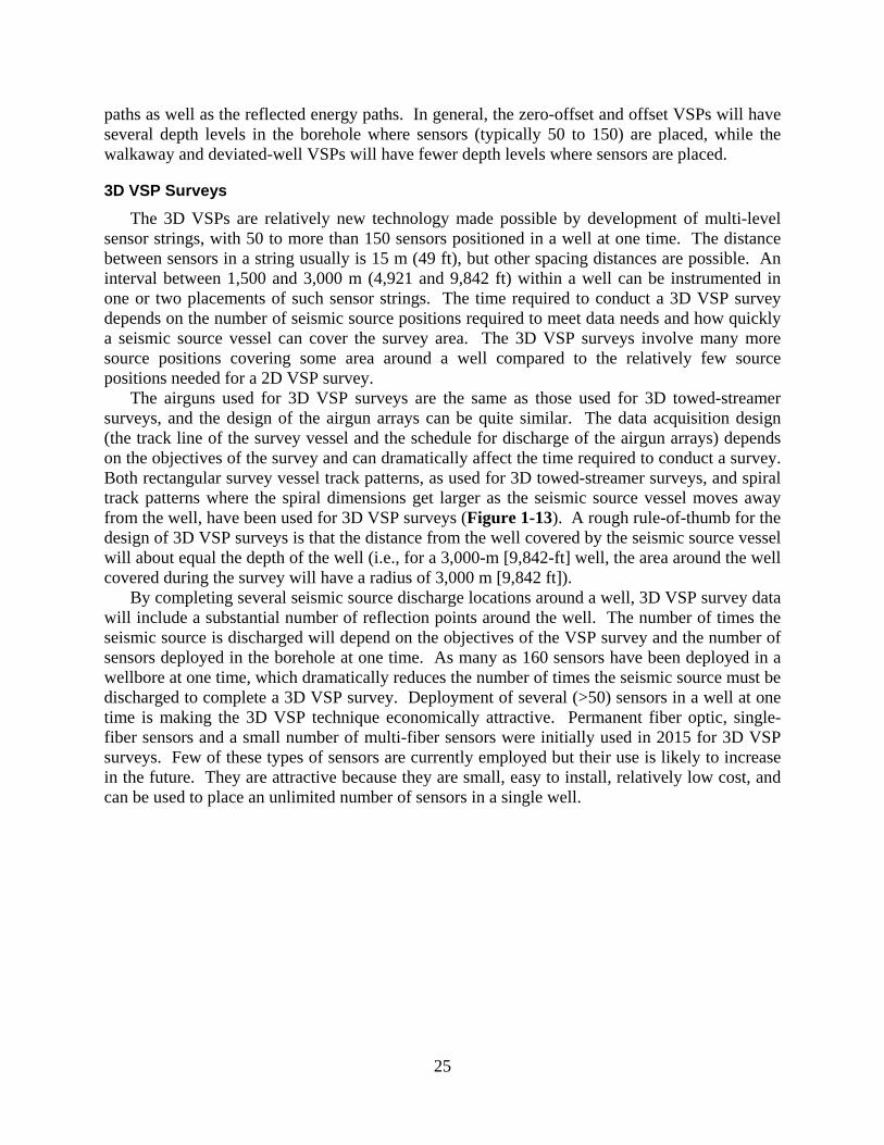
The subsurface image obtained from a VSP survey will be a 2D plane defined by the source location and the borehole (Figure 1-13). In Figure 1-12, the black arrows indicate ray paths for energy that propagates from the seismic source directly to each sensor in a borehole. The red arrows indicate ray paths for energy that is reflected from some point in the subsurface to sensors in the borehole. For the deviated-well VSP, the red ray paths show the directly arriving energy

25

paths as well as the reflected energy paths. In general, the zero-offset and offset VSPs will have several depth levels in the borehole where sensors (typically 50 to 150) are placed, while the walkaway and deviated-well VSPs will have fewer depth levels where sensors are placed.

3D VSP Surveys

The 3D VSPs are relatively new technology made possible by development of multi-level sensor strings, with 50 to more than 150 sensors positioned in a well at one time. The distance between sensors in a string usually is 15 m (49 ft), but other spacing distances are possible. An interval between 1,500 and 3,000 m (4,921 and 9,842 ft) within a well can be instrumented in one or two placements of such sensor strings. The time required to conduct a 3D VSP survey depends on the number of seismic source positions required to meet data needs and how quickly a seismic source vessel can cover the survey area. The 3D VSP surveys involve many more source positions covering some area around a well compared to the relatively few source positions needed for a 2D VSP survey.

The airguns used for 3D VSP surveys are the same as those used for 3D towed-streamer surveys, and the design of the airgun arrays can be quite similar. The data acquisition design (the track line of the survey vessel and the schedule for discharge of the airgun arrays) depends on the objectives of the survey and can dramatically affect the time required to conduct a survey. Both rectangular survey vessel track patterns, as used for 3D towed-streamer surveys, and spiral track patterns where the spiral dimensions get larger as the seismic source vessel moves away from the well, have been used for 3D VSP surveys (Figure 1-13). A rough rule-of-thumb for the design of 3D VSP surveys is that the distance from the well covered by the seismic source vessel will about equal the depth of the well (i.e., for a 3,000-m [9,842-ft] well, the area around the well covered during the survey will have a radius of 3,000 m [9,842 ft]).

By completing several seismic source discharge locations around a well, 3D VSP survey data will include a substantial number of reflection points around the well. The number of times the seismic source is discharged will depend on the objectives of the VSP survey and the number of sensors deployed in the borehole at one time. As many as 160 sensors have been deployed in a wellbore at one time, which dramatically reduces the number of times the seismic source must be discharged to complete a 3D VSP survey. Deployment of several (>50) sensors in a well at one time is making the 3D VSP technique economically attractive. Permanent fiber optic, single-fiber sensors and a small number of multi-fiber sensors were initially used in 2015 for 3D VSP surveys. Few of these types of sensors are currently employed but their use is likely to increase in the future. They are attractive because they are small, easy to install, relatively low cost, and can be used to place an unlimited number of sensors in a single well.

26

Figure 1-13. The Geometry of a 3D VSP Survey.

Checkshot Surveys

Checkshot surveys are similar to a zero-offset VSP surveys but (1) are less complex and require less time to conduct, (2) produce less information, (3) are cheaper, (4) use a less sophisticated borehole seismic sensor, and (5) acquire shorter data records at fewer depths. During a checkshot survey, a seismic sensor is sequentially placed at a few depths (<20) in a well, and a seismic source (almost always an airgun) is hung from the side of the well platform (Figure 1-14). Only the first energy arriving at the sensor from the seismic source is permanently recorded by the sensor and recording unit combination (the black arrow in Figure 1-14 indicates a ray path for energy propagating from the source directly to a sensor positioned in the borehole). No reflection events are recorded, and no sophisticated data processing like that for VSP surveys is required. The purpose of a checkshot survey is to estimate the velocity of sound in rocks penetrated by the well. Typically, the depths at which the sensors are placed are at, or near, the boundaries of prominent lithologic features. Checkshot surveys can be conducted quite quickly, much quicker than VSP surveys, but they produce much less information. Because checkshot surveys are much less expensive and do not use the wellbore and the drilling rig as long, they are much more common than VSP surveys.

In most checkshot surveys, the seismic source is hung from the platform in a fixed location within the water column, so a surface vessel is not needed. Because reflection energy does not need to be acquired, the seismic source usually is smaller than those used for VSP surveys. On occasion, the availability of seismic sources and logistics sometimes makes it operationally and financially advantageous to use a VSP type of seismic source array.

27

Figure 1-14. The Geometry of a Checkshot

Survey.

Seismic While Drilling

The acquisition of seismic while drilling refers to the acquisition of borehole data while there is downtime from the actual drilling. There are two different modes of acquisition. One mode collects data when a stand of pipe (90 or 135 ft; 27 or 41 m) is being connected to the drill stem. These surveys can take days to a month to complete, but they are done intermittently during that time period. Airgun arrays are 19,665 to 25,564 cm3 (1,200 to 1,560 in3). The other mode collects borehole data during the time while round tripping all drill pipe out of the borehole to change the bit. This survey is run intermittently for weeks and sometimes up to a month to the well completion depth.

Vertical Cable Surveys

Vertical cable surveys use hydrophones positioned along a cable held vertically in the water column between a seafloor anchor and a buoy at the sea surface. The hydrophones record the energy produced by an acoustic seismic source, typically an airgun array. The primary energy of interest is reflections from subbottom geological features. This technique produces a VSP without using a well, but it requires two vessels: one to manage the hydrophone cables and one to manage the seismic sources.

28

The objectives of the survey determine the number and positions of hydrophone cables and seismic sources. The hydrophone cables may be left in place for hours or days, depending on the size of the survey area and operating conditions. The airgun array is the same as that used for 3D towed-streamer surveys. These types of surveys are not common because of the better data acquisition techniques available using other types of surveys.

4D Time-Lapse Surveys

The 4D surveys are repeated one or more times after the original baseline survey has been completed. The purpose of 4D surveys is to monitor reservoir changes in a producing field. For approximately 25 years, the purpose of 4D surveys in the hydrocarbon industry has been to monitor changes in oil and gas reservoirs to better manage them. However, in addition to that purpose, 4D surveys now are being used to monitor changes for environmental and safety reasons. Examples of this include monitoring for oil leaks in the seafloor above reservoirs not only for health, safety, security, and environment purposes but also for carbon capture and storage. Some of the survey types described in this section can be used in time-lapse mode, including VSP, 3D towed-streamer, and multibeam bathymetry.

The usefulness and value of 4D surveys is well-established, and such surveys have become common. The particular acquisition technique chosen (towed-streamer, temporary OBCs or OBNs, or permanently emplaced systems on the seafloor) depends on the objectives of the survey, the particular geology being addressed, the physical facilities in a given field, and the nature of the geophysical response to changes such as reservoir saturation and pressure. The seismic sensors used for 4D surveys have been almost exclusively nodal. The seismic survey equipment and procedures used for 4D surveys are the same as those described in previous sections for 3D surveys. However, because these surveys are conducted over producing fields, the survey area is smaller and the survey time shorter than needed for most other 3D towed-streamer and 3D OBCs or OBNs surveys. The time lapse between a baseline survey and 4D survey has been as short as 3 months and as long as 10 years. Many 4D surveys are repeated every 1 to 2 years. When permanently emplaced receiver systems are used, the repeat time generally is on the order of several months because a relatively small and inexpensive seismic source vessel is all that is required to conduct additional monitoring surveys. A key requirement of 4D surveys is acquisitional repeatability, with emphasis on controlling factors that could confound results. This means the monitoring surveys use the same seismic source size and depth as well as the same receiver systems and attempt to duplicate as much as possible all other details of the original survey.

1.3 HIGH-RESOLUTION GEOPHYSICAL SURVEYS Before any operation takes place on the seafloor, there is an operational and legal regulatory

need to characterize the nature of the seafloor and the geologic layers immediately beneath it. The HRG surveys are conducted to investigate the shallow subsurface for geohazards and soil conditions over specific locations in one or more OCS lease blocks. Identification of geohazards is necessary to avoid drilling and facilities emplacement problems. Geohazards include shallow gas, over-pressured zones, shallow water flows, shallow buried channels, gas hydrates, incompetent sediments, and mass transport complexes. These surveys also are used to identify potential benthic biological communities (or habitats) and archaeological resources. Survey data are used for initial site evaluation, drilling rig emplacement, and platform or pipeline design and emplacement. The HRG surveys and reporting requirements are outlined by Notice to Lessees

29

and Operators (NTL) 2008-G05 (“Shallow Hazards Program,” extended with NTL 2014-G03; USDOI, BOEM, 2008) and NTL 2005-G07 (“Archaeological Resource Surveys and Reports”; USDOI, BOEM, 2005).

In most cases, conventional 2D and 3D deep-penetration seismic surveys do not have the correct resolution to provide the required information. Although HRG surveys may use a single airgun source, they generally use electromechanical sources such as side-scan sonars, shallow- and medium-penetration subbottom profilers, and single-beam echosounders (SBESs) or multibeam echosounders (MBESs). The sections to follow describe these sources and techniques.

1.3.1 Airgun High-Resolution Geophysical Surveys This section discusses shallow-penetration airgun seismic surveys used for HRG surveys.

Because the intent of high-resolution, shallow-penetration airgun seismic surveys is to image shallow depths (typically 1,000 m [3,280 ft] or less below the seafloor) and to produce high-resolution images, the airgun sources used (typically 1 or 2 airguns) are smaller (typically 40 to 400 in3), the streamers are shorter and towed shallower, the streamer-separation distances are smaller (150 to 300 m [492 to 984 ft]), and the firing times between airgun shotpoints are shorter than for conventional 2D and 3D airgun seismic surveys. Typical surveys cover one OCS lease block, which is usually 4.8 km (3 mi) on a side. The presence of historic archaeological resources (e.g., shipwrecks), shallow hazards, or live bottom features can require surveys using a maximum line spacing of 300 m (984 ft). Including vessel turns at the end of lines, the time required to survey (transect all lines) one OCS lease block is approximately 36 hr. Other activities before and after the time spent actively acquiring seismic data, such as streamer and airgun deployment and other operations, add to the total survey time. In addition, weather can create conditions that degrade the performance of streamer arrays and prevent acquisition of useful data, especially in shallow water where streamers are towed close to the sea surface. Sea state conditions caused by weather in the GOM can result in operational downtime. Also, in some instances, the time required to conduct a survey is affected by needs for tighter line spacing to accomplish survey objectives and data quality.

The 3D high-resolution airgun seismic surveys using ships towing multiple streamer cables have become more common. These surveys include (1) dual-source acquisition that incorporates better source and streamer positioning accuracies (derived from GPS) that allow for advanced processing techniques (pre stack time migration), (2) single-source multi-streamer (up to 6 streamers maximum in most cases), (3) dual-source multi-streamer, and (4) P-Cable acquisition. All of these 3D survey types, except P-Cable acquisition, have the same surveying practices as high-resolution 2D surveying, including shorter streamers (typically 100 to 1,200 m [328 to 3,937 ft]); shallower streamer tow depths; more closely spaced shots, often as close as 12.5 m (41 ft); smaller airgun arrays (typically 40 to 400 in3); and more closely spaced track lines (generally 25 to 100 m [82 to 328 ft]).

The P-Cable acquisition survey technique was first tested in 2007 and utilized in 2014 for the first multi-client geohazards ultra-high-resolution 3D (UHR3D) survey in the GOM. In a UHR3D survey, a cable is towed oriented perpendicular to the ship track (Figure 1-15). Attached to the cable are a series (10 to 20) of short (25 to 300 m [82 to 984 ft]), closely spaced (12.5 m [41 ft]) streamers. The UHR3D surveying requires accurate geological positioning. Figure 1-16 shows the level of detail of the seafloor morphology and of the subsurface below the seafloor provided by UHR3D technology for five examples of geohazards. It should be noted

30

that the subsurface velocities required to process the P Cable (and similar technologies) cannot be obtained from this acquisition technique; instead, it must be obtained from borehole checkshot surveys (refer to Section 1.2.1.5) or other methods that measure the appropriate velocities (Hill et al., 2015).

Figure 1-15. The Equipment Layout for a P-Cable Acquisition Survey.

31

Figure 1-16. Examples of the Data that the P-Cable Technology can Deliver. Diagrams (A) and (B)

Show the Seafloor Morphology in Two Areas of the Gulf of Mexico and the Locations of Features (C) Through (G) Whose Vertical Structures are Shown at the Bottom (From: Brookshire and Scott, 2015).

32

1.3.2 Non-Airgun Acoustic High-Resolution Geophysical Surveys Typical non-airgun HRG surveys may involve one or more types of high-frequency acoustic

sources, such as the following:

• subbottom/sediment profilers (2.5 to 7 kHz); o pingers (2,000 Hz); o sparkers (50 to 4,000 Hz); o boomers (300 to 3,000 Hz); o compressed high-intensity radar pulse (CHIRP) subbottom profilers (4 to

24 kHz); o side-scan sonar (usually 16 to 1,500 kHz);

• single-beam echosounders (12 to 240 kHz); and

• multibeam echosounders (50 to 400 kHz).

In general, any combination of these techniques, which are employed for both hazard and archaeological surveys, may be conducted during a single deployment from the same vessel. However, conventional 3D seismic data generally cannot be substituted for HRG survey data for pipeline pre-installation surveys. The vessel tow speed during non-airgun HRG surveys may be up to 4 to 5 kn (4.6 to 5.8 mph). If a high-resolution airgun survey is required to meet the survey objective, it makes operational/economic sense to do everything in a single deployment. For postlease engineering studies used to guide the placement of production facilities and pipelines in deep water and to meet archaeological requirements, HRG surveys often are conducted with autonomous underwater vehicles (AUVs) equipped with side-scan sonar, an MBES, and a subbottom profiler. Geophysical contractors have been using AUVs since 2000 to make detailed maps of the seafloor before installing subsea infrastructure.

1.3.2.1 Subbottom Profiling Surveys

Sparker

A sparker is an acoustic source that uses electricity to vaporize water, creating collapsing bubbles that produces a broadband (50 Hz to 4 kHz) omnidirectional pulse of sound that can penetrate a few hundred meters (several hundred feet) into the subsurface. Because of the sparker’s relatively high frequency compared to deep-penetration seismic, it is used for high-resolution shallow imaging. Short hydrophone arrays towed near the sparker receive sound reflected from subsurface features. Normally, the sparker is towed on one side of a ship’s wake and the hydrophone array is towed on the other side. Some of the operational characteristics of sparker surveys are as follows:

• sparker and hydrophone array tow depths are 1 to 1.5 m (3 to 5 ft);

• vessel speed is 3 to 6 kn (3.5 to 6.9 mph) (similar to seismic), but can be faster;

• acquired reflection return length typically is 500 millisecond (ms) (shorter than seismic);

33

• operating rate of two discharges per second (faster than seismic);

• analog-to-digital sampling interval of 0.1 to 0.25 ms (higher than seismic); and

• dominant sound frequency band is 300 to 800 Hz (higher than seismic).

Boomer

A boomer is an acoustic sound source that uses electricity to cause two spring-loaded plates to rapidly repel each other, generating an acoustic pulse. The acoustic pulse has a bandwidth of 300 Hz to 3 kHz. A boomer is commonly mounted on a sled and towed behind a vessel. Short hydrophone arrays towed nearby receive sound reflected off subbottom features. Depending on subsurface geology, the resolution of the boomer system typically is 0.5 to 1 m (1.6 to 3 ft) and penetration is 25 to 50 m (82 to 164 ft). Boomers generate a sound pulse with very repeatable characteristics, although wave motion can distort the signal. A boomer often is deployed with other higher frequency systems to increase the depth range achieved by the survey.

Pingers and CHIRP Subbottom Profilers

The acoustic pinger is the oldest technology used for bathymetric and subbottom profiling surveys. A pinger operates at a single frequency (usually 2 kHz) and is a relatively weak sound source, penetrating to a maximum depth of approximately 5 m (16 ft), depending on the composition of seafloor sediments.

CHIRP is a type of sonar used for high-resolution sub-bottom profiling. The word is an acronym for Compressed High-Intensity Radiated Pulse. Instead of sending a single frequency, CHIRP sends a continuous sweep of frequencies ranging from 500 Hz up to 24 kHz approximately every 0.5 to 1 seconds. CHIRP sonar technology then interprets frequencies individually upon their return. Because this continuous sweep of frequencies provides CHIRP with a much wider range of information, it is able to create a much clearer, higher-resolution image than the older subbottom profiling methods while achieving the same or better depth of penetration. CHIRP systems are used for high-resolution mapping of relatively shallow deposits and have less penetration than boomers; however, newer CHIRP systems are able to penetrate to levels comparable to boomers yet yield extraordinary resolution of the substrate (NSF and USDOI, GS, 2011).

Side-Scan Sonars

Sonar uses reflections of sound pulses to locate, image, and aid in the identification of objects in the water and on the seafloor, and to determine water depth. Side-scan sonars transmit sound pulses in a beam that is narrow in the direction along the tow vessel’s track and wide vertically. The fan-shaped transmit beam sweeps the seafloor from directly under the sound source to either side, typically to a distance of 50 to 200 m (164 to 656 ft). The sound pulses do not penetrate the subbottom but are reflected off the seafloor and objects lying on the seafloor. As the vessel moves forward, an image of the seafloor and the relative size and location of objects on the seafloor to either side of the vessel is created. Side-scan sonar typically consists of three components: a towfish that contains the sound source and receiving transducers; a transmission cable; and a topside echo signal processing and display unit. Side-scan sonars often are used in conjunction with a SBES or MBES system that covers the part of the seafloor directly under the survey vessel that is not covered by the side-scan sonar. Because these types of sonars

34

are used to detect relatively small objects, they operate at higher frequencies (1 to 1,500 kHz), and because of the high attenuation of high-frequency sound in the ocean, these sonars have useful ranges of a few hundred meters or less. There are hull-mounted and towed side-scan sonars, but because they operate at higher frequencies and their range is limited, imaging the seafloor in water depths greater than 10 m (33 ft) requires the use of a towed body or an AUV to position the side-scan sound source and receiving transducers closer to the seafloor.

1.3.2.2 Echosounders Echosounders, also called depth sounders and fathometers, are used to estimate water depth.

Most seismic and HRG survey vessels have an echosounder, which works by emitting a short, usually single frequency, pulse of sound and receives, processes, and displays echo returns from the seafloor. If the speed of sound in sea water is known, the device can estimate water depth by multiplying the speed of sound by half the time from transmit of a pulse to receipt of an echo. Many echosounders also have sensors that detect salinity, temperature, and conductivity, measurements that are used to estimate the speed of sound in water.

Single-Beam Echosounders

An SBES transmits a sound pulse aimed vertically below the vessel to estimate the distance to the seafloor directly beneath the ship. Typically, higher operating frequencies are used for shallow depths and lower frequencies are used for greater depths. For example, an echosounder operating at 200 kHz would be used in shallow (<100 m [328 ft]) water, and an echosounder operating at 3 kHz would be used in very deep water (3,000 m [9,842 ft]). If a high level of detail about seafloor depths is needed, a survey vessel must complete many closely spaced track lines because depth is only estimated directly beneath the ship.

Multibeam Echosounders

The MBESs emit multiple sound beams in a fan shape, covering a range of angles beneath the ship orthogonal to the ship’s track. Therefore, in one pass of the survey vessel over an area, the bathymetry of a swath of the seafloor is estimated, so a larger area can be covered in a shorter time and with fewer track lines than is possible using an SBES. The width of the swath depends on the number of sound beams, the multibeam operating frequency, and water depth. The MBESs that operate at low frequencies (e.g., 12 kHz) are used to survey at depths up to 10,000 m (32,808 ft) while others operating at high frequencies (e.g., >300 kHz) are used to survey at depths as shallow as 20 m (66 ft) or less.

35

2 THE DATE(S) AND DURATION OF SUCH ACTIVITY AND THE SPECIFIC GEOGRAPHICAL REGION WHERE IT WILL OCCUR

Oil and gas activity on the OCS of the northern GOM (U.S. waters north of the Exclusive Economic Zone [EEZ] boundary) is in a mature state, although large discoveries are expected in deeper waters. The eastern GOM remains largely under explored. New seismic survey activity is expected to occur in the Eastern Planning Area (EPA); however, industry activity in the EPA has historically been limited to the westernmost portions of the planning area due to lack of availability of acreage for lease and is usually defined by the Five-Year Program (see http://www.boem.gov/Five-Year-Program/).

Proposed Action

The proposed action in this petition is BOEM’s request for authorization under the Marine MMPA (16 U.S.C. §§ 1361 et seq.) for the “take” of marine mammals incidental to geophysical activities conducted by the oil and gas industry in the northern GOM waters (U.S. waters north of the EEZ boundary) via an ITR with subsequent LOAs sought by industry. State-of-the-practice data about the ocean bottom and subsurface data are collected through geophysical activities to provide information about the potential location and extent of oil and gas reserves. Access to and the use of the best available information obtained from geophysical activities helps to make informed business, management, design, stewardship, and environmental protection decisions. Such decisions are an integral part of several Bureau of Ocean Energy Management’s OCS programs, including oil and gas (e.g., location, extent, fair market value of resources, and orderly development of hydrocarbon reserves) and to industry.

Proposed Action Scenario

Typical prelease activities include deep-penetration seismic airgun surveys to explore and evaluate deep geologic formations. The 2D seismic surveys are usually designed to cover thousands of square miles or entire geologic basins as a means to geologically screen large areas for potential hydrocarbon prospectivity. The 3D surveys can consist of several hundred OCS lease blocks and provide much better resolution to evaluate hydrocarbon potential in smaller areas or specific prospects. Other prelease surveys include largely passive data gathering methods such as electromagnetic, gravity, and magnetic surveys, as well as remote-sensing surveys from aircraft and satellites.

Postlease activities conducted by operators can include additional seismic surveys, non-airgun HRG seismic surveys, and seafloor sampling (including stratigraphic wells, shallow test wells, and geotechnical sampling). Examples of postlease seismic surveys include VSPs with geophone receivers placed in a wellbore and 4D (time-lapse) surveys to monitor reservoirs during production. Non-airgun HRG surveys are conducted in leases and along pipeline routes to evaluate the potential for geohazards, archaeological resources, and certain types of benthic communities. Prelease and postlease activities are described further in Section 1.

Projected Activity Levels

To construct a scenario for geophysical surveys in support of oil and gas exploration, BOEM evaluated recent trends in permit applications as well as industry estimates of future seismic survey activity. The scenario to follow is programmatic in nature and forward-looking, with the

36

fluctuating market influencing the amount, timing, and location of surveys in any given year. It is not meant to be exact but rather an informed upper estimate of future survey activity.

Given the programmatic and predictive nature of the scenario, defining specific locations of each survey is not possible. Specific surveys may span 1 day, weeks, or months (and a single deep-penetration seismic survey may last over a year). Activity levels and frequency are expected to be relatively constant throughout the year (little variation in regards to seasonality) but are likely to vary, sometimes greatly, between years. Activity levels are also estimated to be spread mostly throughout the Western and Central Planning Areas (WPA and CPA) with some limited activity in the EPA (Figure 2-1). These planning areas and administrative boundaries represent the largest area within which surveys may occur and are the starting point of the development of the scenario.

Figure 2-1. BOEM’s Gulf of Mexico Planning Areas and Proposed 2017-2022 Lease Sale Areas.

In order to better frame activity levels for the purposes of this petition and acoustic modeling,

the planning areas and administrative boundaries above were divided into seven acoustic zones based on the physical properties of the project area and the distribution of its marine mammals. This included three shelf zones, three slope zones, and 1 deep zone (Figure 2-2 and Appendix A.

37

Figure 2-2. Seven Acoustic Regions and Representative Model Sites (Zones) in the Gulf of Mexico.

Finally, within each of the seven acoustic zones, activity levels were projected on an annual

basis by the number of days (24-hr periods) per survey type over the course of a 5-year MMPA rulemaking (2018-2022; Table 2-1).

Table 2-1. Projected Level of Effort in Days (24 h) for Survey Types in Years 2018 to 2022 (expected

years covered under an MMPA rule) The 2-D seismic survey is 131,097 cm3; 8000 in3 airgun array with 1 vessel. 3-D seismic survey is 131,097 cm3; 8,000 in3 airgun array with 2 vessels. The WAZ seismic survey is 131,097 cm3; 8,000 in3 airgun array with four vessels. Coil seismic survey is 131,097 cm3; 8,000 in3 airgun array with 4 vessels. Shallow hazards seismic survey is a 1,475 cm3; 90 in3 airgun. The high-resolution sources include for side-scan sonar, multibeam, and sub-bottom profiler. The VSP is 31,097 cm3; 8,000 in3 airgun array with 1 vessel.

Year Zone 2-D 3-D WAZ Coil Shallow Hazards Boomer High-Resolution

Sources VSP

2018

1 0 0 0 0 0 0 1 0 2 0 243 0 0 2 0 18 0 3 0 0 0 0 0 0 4 0 4 0 0 0 0 0 0 1 0 5 0 342 160 69 0 0 27 2 6 0 186 49 21 0 0 12 0 7 0 456 208 89 0 0 36 2

2019

1 0 0 0 0 0 0 0 0 2 0 364 43 19 2 1 16 0 3 0 30 0 0 0 0 3 0 4 66 61 21 9 0 0 1 0 5 28 247 96 41 0 0 27 2 6 0 99 0 0 0 0 12 0 7 94 380 140 60 0 0 36 2

38

2020

1 0 0 0 0 0 0 0 0 2 0 243 0 0 0 0 20 0 3 0 0 0 0 0 0 3 0 4 0 92 0 0 0 0 0 0 5 0 295 192 82 2 1 25 2 6 0 99 0 0 0 0 13 0 7 0 467 241 103 3 2 34 3

2021

1 0 0 0 0 0 0 0 0 2 0 364 43 19 0 0 18 0 3 0 0 0 0 0 0 2 0 4 0 92 0 0 0 0 1 0 5 0 247 160 69 0 0 30 2 6 0 186 49 21 0 0 13 0 7 0 421 208 89 0 0 40 3

2022

1 0 0 0 0 0 0 0 0 2 0 243 0 0 0 0 16 0 3 0 30 0 0 0 0 2 0 4 33 61 21 9 0 0 1 0 5 28 247 160 69 0 0 32 2 6 0 99 0 0 0 0 13 0 7 64 380 220 94 0 0 43 3

Total 313 5,974 2,011 863 9 4 500 23

There is no way to provide an exact number of what the above total day/hr equate to for the number of each type of survey. Not all surveys, even within the same type category, are created equal (i.e., not every deep-penetration seismic airgun survey happens within the same amount of effort days). Further, there is fluctuation and variability within the financial market and individual company needs that can greatly affect the amount of effort (survey days) and number of survey types in any given year. As an example, Table 2-2 provides a history of the annual variability as a guidepost. It reflects actual permitted/approved surveys for 2006-2016 into two bins: deep-penetration seismic surveys with airguns (2D, 3D, WAZ, Coil, VSP) and HRG surveys (shallow hazard, boomer, high-resolution sources). Between 2006 and 2015, the deep-penetration seismic surveys ranged from 21 to 34, but there have only been 2 permitted surveys in 2016 so far. The same trend can be seen for HRG surveys. In some years, HRG surveys ranged up to 78 surveys, while in 2016, there were 7 HRG surveys. The lower number of HRG surveys from 2011 to 2013 is related to decreased activity levels post-Deepwater Horizon. The lower number of both bins of surveys in 2016 is related to the more recent downward trend in the price of oil and the subsequent self-reduction of survey requests from industry. It is difficult to determine if this downward trend will continue or if the number of surveys requests will increase within the 5-year time span of any issued Marine Mammal Protection Act ITR.

39

Table 2-2. Permitted Surveys in the Gulf of Mexico for 2006-2016

Year Deep Penetration Seismic

with Airguns (2D, 3D, WAZ, Coil, VSP)

Shallow Hazard and High-Resolution Surveys Total

2006 30 48 78 2007 34 70 104 2008 20 78 98 2009 22 39 61 2010 26 32 58 2011 24 2 26 2012 29 8 37 2013 24 14 38 2014 28 39 67 2015 21 38 59 2016 2 7 9

BOEM has, therefore, decided to maintain the original scenario (described in Table 2-1 above) recognizing that it likely represents the upper end of likely survey activity in any given year and would accommodate flexibility for market influences. In developing the scenario, BOEM also has taken into account the restrictions under the Gulf of Mexico Energy Security Act (GOMESA), which precludes leasing, preleasing, or any related activity in all areas in the GOM east of the Military Mission Line (86°41’ W. longitude), and the area within the CPA that is within 125 mi (201 km) of Florida. The GOMESA restrictions place most of the EPA and a portion of the CPA under restriction from oil and gas leasing until 2022, which is within the time period covered by this petition (USDOI, BOEM, 2006). However, geophysical surveys are not restricted by GOMESA.

40

3 THE SPECIES AND NUMBERS OF MARINE MAMMALS LIKELY TO BE FOUND WITHIN THE ACTIVITY AREA; AND

4 A DESCRIPTION OF THE STATUS, DISTRIBUTION, AND SEASONAL DISTRIBUTION (WHEN APPLICABLE) OF THE AFFECTED SPECIES OR STOCKS OF MARINE MAMMALS LIKELY TO BE AFFECTED BY SUCH ACTIVITIES

The GOM is a semi-enclosed marginal sea of the Atlantic Ocean bounded by the United States, Mexico, and Cuba. Entry from the Atlantic Ocean into the GOM is gained through the Straits of Florida, and entry from the Caribbean Sea is gained through the Yucatan Channel. The GOM is characterized by a very wide, gently sloping continental shelf around most of its margin. The only area of the U.S. Gulf (north of the EEZ) where the water depth reaches 200 m (656 ft) within 50 km (31 mi) of the shore is off the Mississippi River delta. Continental shelf waters (<200 m; 656 ft deep) comprise about 35 percent of the GOM surface, and continental slope waters (200-3,000 m; 656-9,843 ft) make up another 40 percent (Wursig et al., 2000). In contrast to the smooth, gentle slope of the continental shelf, the GOM continental slope is steep and irregular with canyons and knolls. The remaining 25 percent of the GOM waters includes the abyssal depths, mainly of the Sigsbee Abyssal Plain.

The U.S. GOM marine mammal community is diverse and distributed throughout the northern Gulf waters. Table 3-1 lists the individual species that routinely inhabit the United States GOM and, thus, might be affected by the subject activities. Mullin and Fulling (2004) reported that many of these species were widely distributed but some had a more regional distribution and these are noted in species accounts. It was also reported that there was some evidence of seasonal changes in slope waters species abundance but that the Gulf marine mammal community remained diverse and abundant throughout the year and no commonly occurring species vacated the slope waters seasonally (Mullin et al., 2004). Seasonal observations are also reported under individual species accounts.

Slope waters are routinely inhabited by 20 species, most of which have worldwide distribution in deep, warm-temperate to tropical waters. Two exceptions to worldwide distributions are Atlantic spotted dolphins (Stenella frontalis) and Clymene dolphins (Stenella clymene). Common in the GOM, these two species are endemic to the Atlantic and its associated waters. The only two species that are commonly found in continental shelf waters are bottlenose dolphins (Tursiops truncatus) and Atlantic spotted dolphins (Stenella frontalis) (Fulling et al., 2003).

There are species that have been reported from GOM waters, either by sighting or stranding, that are not included in the species accounts because the observations were not such that would deem the species extralimital in the GOM (Wursig et al., 2000; Mullin and Fulling, 2004; Robert et al., 2016). These species include the blue whale (Balaenoptera musculus), the North Atlantic right whale (Eubalaena glacialis), and the Sowerby’s beaked whale (Mesoplodon bidens), all considered extralimital in the GOM, and the humpback whale (Megaptera novaeangliae), the fin whale (Balaenoptera physalus), the sei whale (Balaenoptera borealis), and the minke whale (Balaenoptera acutorostrata), all considered rare occasional migrants in the northern GOM. The National Oceanic and Atmospheric Administration's (NOAA) Stock Assessment Reports also list them as extralimital. Because of the rarity of these species in the GOM, no potential effects from subject activities are expected and they are not considered further in this petition.

41

BOEM does note that fin whales were included within density estimates from Roberts et al. (2016). However, Roberts et al. (2016) states that, “In the GOM, surveys reported on-effort sightings of only two baleen whale species. A single fin whale was sighted in the western Gulf at the shelf break. Fin whales do not inhabit the northern GOM, but the process was to model all species reported while observers were on effort, regardless of rarity; accordingly, we incorporated this extralimital sighting into a GOM-wide stratified model.” Given this clarification, BOEM agrees that fin whales are extralimital in the GOM and is not including them in this petition.

Species/Stocks Potentially Affected by the Proposed Action and Abundance Estimates

After reviewing available information on GOM marine mammals, BOEM has determined that 21 species/stocks of marine mammals are expected to be found in the activity area and may be potentially affected by the proposed action. These species are noted in Table 3-1 along with a summary of their expected status, occurrence, seasonality, range and abundance.

Prior to the start of the acoustic modeling described in Appendix A, a decision had to made on which abundance estimates should be used for the affected marine mammal species/stocks. The two choices were as follows:

(1) NOAA Stock Assessment Reports for the Northern GOM (Waring et al., 2016): Methodology is based on actual sightings data; and

(2) Habitat density modeling performed by Duke University (Roberts et al., 2016): Methodology is based on interpreting sightings data but also incorporating habitat modeling to predict species occurrence, seasonality, and abundance.

Based on direction from NMFS, the abundance estimates generated by the Duke Habitat Density Modeling (#2 above, Roberts et al., 2016) were used for the purposes of acoustic modeling associated with this petition. Except for Table 3-1, which provides abundance estimates based on both methodologies (for comparison purposes), the remainder of this petition will refer only to predictive abundance and density models from the Duke Habitat Density Modeling.

42

Table 3-1. Population Estimates for Marine Mammal Species Likely to be Found in the Proposed Activity Area

Species Status Occurrence Seasonality Range Abundance

Atlantic Spotted Dolphin (Stenella frontalis)

MMPA-Protected ESA-N/A

Northern Gulf All Seasons

Continental shelf waters 10-200 m deep to slope waters <500 m deep

47488-DUKE Unknown-NOAA

Beaked whales Cuvier’s (Ziphius cavirostris) Blainville’s (Mesoplodon densirostris) Gervais’ (Mesoplodon europaeus)

MMPA-Protected ESA-N/A

Northern Gulf All Seasons >500 m deep and deep oceanic

2910-DUKE (combined stocks) NOAA (separated by stock) Cuvier’s Beaked Whale 74 Blainville’s Beaked Whale 149 Gervais’ Beaked Whale 149

Bottlenose Dolphin (Turisops truncatus)

MMPA-Protected ESA-N/A

Northern Gulf All Seasons

138,602-DUKE (entire GOM species) NOAA (published by stock) Continental-51,192 Eastern Coastal-12,388 Northern Coastal-7,185 Western Coastal-20,161 Oceanic- 5,806 GOM Bay, Sound, and Estuary-unknown for all but 6 stocks Barataria Bay- unknown Mississippi

43

Sound-901 St. Joseph Bay-152 Choctawhatchee Bay-179

Bryde’s whale (Balaenoptera edeni)

MMPA-Protected ESA-Status Review

Northeastern Gulf

Spring Sightings, Year-Round Strandings

Northeastern Gulf, outside the 100-m isobaths

44-DUKE 33-NOAA

Clymene dolphin (Stenella clymene)

MMPA-Protected ESA-N/A

Northern Gulf

Winter, Spring, and Summer based on surveys

Oceanic and to a lesser extent continental shelf waters in the northern Gulf

11000-DUKE 129-NOAA

False killer whale (Pseudorca crassidens)

MMPA-Protected ESA- N/A

Northeastern Oceanic Gulf

Recent sightings in spring and summer

Oceanic Gulf 3204-DUKE Unknown-NOAA

Fraser’s dolphin (Lagenodelphis hosei)

MMPA-Protected ESA- N/A

Northern Gulf All Seasons Oceanic Gulf >200m

1665-DUKE Unknown-NOAA

Killer whale (Orcinus orca)

MMPA-Protected ESA- N/A

North-Central Oceanic Gulf

Recent sightings in summer

256-2,652 m (based on sightings)

185-DUKE 28-NOAA

Kogia spp. (Dwarf sperm whale (Kogia sima) and Pygmy sperm whale (Kogia breviceps))

MMPA-Protected ESA-N/A

Oceanic Gulf All Seasons Oceanic Gulf 2234-DUKE 186-NOAA

Melon-headed shale (Peponocephala electra)

MMPA-Protected ESA- N/A

Northern Gulf All Seasons

>800 m and west of Mobile Bay, Alabama

6733-DUKE 2235-NOAA

Pantropical spotted dolphin (Stenella attenuatus)

MMPA-Protected ESA-N/A

Northern Oceanic Gulf All Seasons Oceanic Gulf 84014-DUKE

50880-NOAA

Pygmy killer whale (Feresa attentuata)

MMPA-Protected ESA-N/A

Oceanic Gulf All Seasons Oceanic Gulf 2126-DUKE 152-NOAA

Risso’s dolphin (Grampus griseus)

MMPA-Protected ESA-N/A

Northern Gulf All Seasons

Throughout oceanic waters but concentrated

3137-DUKE 2442-NOAA

44

at continental slope

Rough-toothed dolphin (Steno bredanensis)

MMPA-Protected ESA- N/A

Northern Gulf All Seasons

Oceanic and to a lesser extent continental shelf waters in the northern Gulf

4853-DUKE 624-NOAA

Short-finned pilot whale (Globicephala macrorhynchus)

MMPA-Protected ESA-N/A

Northern Gulf All Seasons Continental slope west of 89˚W.

1981-DUKE 2415-NOAA

Sperm whale (Physeter macrocephalus)

MMPA-Depleted ESA-Endangered

Northern Gulf All Seasons Continental slope and oceanic waters

2128-DUKE 763-NOAA

Spinner dolphin (Stenella longirostris)

MMPA-Protected ESA-N/A

Northern Oceanic Gulf All Seasons

Generally east of the Mississippi River

13485-DUKE 11441- NOAA

Striped dolphin (Stenella coeruleoalba)

MMPA-Protected ESA-N/A

Northern Oceanic Gulf All Seasons Oceanic Gulf 4914-DUKE

1849-NOAA

For the marine mammal species/stocks within the proposed activity area, Table 4-1 provides

the predicted mean density estimates per acoustic zone used in the modeling (refer to Appendix A for methods used to calculate the mean density). These mean density estimates are based on Roberts et al. (2016). The narrative to follow then provides details on each species/stock, distribution, habitat, behavior, vocalization and hearing, threats, and status. Table 4-1. Mean Density Estimates of Marine Mammals in the GOM per Modeled Acoustic Zone

(Figure 2-2 and AppendixA)

Species Zone 1 Mean

Zone 2 Mean

Zone 3 Mean

Zone 4 Mean

Zone 5 Mean

Zone 6 Mean

Zone 7 Mean

Atlantic spotted dolphins 19.561691 7.456256 8.191627 2.781758 2.031142 1.273500 0.000004

Beaked whales 0.000107 0.000003 0.000001 0.725775 1.080930 0.832344 0.519543 Common bottlenose dolphins 37.130025 53.082960 39.405915 11.553444 5.728691 3.342733 0.027482

Bryde’s whales* 0.012267 0.000164 0.000041 0.035179 0.014526 0.013691 0.000000 Clymene dolphins 0.000785 0.000002 0.000000 0.914148 3.416620 4.262516 2.627719 False killer whales 0.123816 0.028735 0.013218 0.727735 0.726846 0.735816 0.748148 Fraser’s dolphins 0.064342 0.014932 0.006869 0.378170 0.377708 0.382369 0.388778 Killer whales 0.000392 0.000177 0.000191 0.013264 0.020153 0.019773 0.077865 Kogia spp. 0.016379 0.000937 0.000187 0.958299 0.726706 0.411093 0.342218

45

Melon-headed whales 0.002691 0.000181 0.000062 1.181967 2.209811 1.890231 1.533612

Pantropical spotted dolphins 0.111202 0.002317 0.000597 21.767563 15.504281 9.864202 26.087947

Pygmy killer whales 0.001253 0.000078 0.000029 0.296539 0.456866 0.476313 0.661113

Risso’s dolphins 0.017854 0.000835 0.000297 1.419280 0.972485 0.794562 0.419790 Rough-toothed dolphins 0.406426 0.394670 0.396268 0.961959 1.050021 0.997906 0.798816

Short-finned pilot whales 0.000262 0.000010 0.000005 0.685525 0.639206 1.249850 0.121555

Sperm whales 0.000150 0.000007 0.000002 0.482223 0.725159 0.486587 0.467025 Spinner dolphins 0.018491 0.000000 0.000000 11.762649 4.154421 0.236570 0.612156 Striped dolphins 0.002602 0.000025 0.000030 0.799246 1.334442 1.091651 1.365036

*Density estimates for Brydes whales reflected above are based on preliminary estimates provided by Duke University at the time of the acoustic modeling and prior to subsequent revisions published in Roberts et al., 2016. These older mean density estimates are contained here given these were used for the take modeling to be discussed later in the petition.

GOM Cetacean Unusual Mortality Event and Deepwater Horizon Impacts

An Unusual Mortality Event (UME) was declared for dolphins and whales (cetaceans) in the northern GOM (Texas/Louisiana border through Franklin County, Florida) from March 2010 through July 2014. Based upon analysis of stranding data and recommendations from the UME investigative team and the Working Group on Marine Mammal Unusual Mortality Events (an advisory group of marine mammal health and biology experts), NOAA declared the northern GOM cetacean UME closed. The majority of cetaceans involved are also the subject of this petition, including the common bottlenose dolphins (Tursiops truncatus), spinner dolphins (Stenella longirostris), Atlantic spotted dolphins (Stenella frontalis), and melon-headed whales (Peponocephala electra). It is important to note, however, that the findings of the Working Group made no mention of seismic activity as a contributing factor to this UME. Information on the UME (and its linkage to the Deepwater Horizon explosion, oil spill, and response) remain important when considering a potential changing baseline of marine mammal abundance and distributions in the GOM.

Although the UME began prior to the Deepwater Horizon explosion, oil spill, and response, the UME investigation and the Deepwater Horizon Natural Resource Damage Assessment (NRDA) have determined that the Deepwater Horizon oil spill resulted in the death of marine mammals and is the most likely explanation of the persistent, elevated stranding numbers in the northern GOM after the spill. The evidence to date supports that exposure to Deepwater Horizon petroleum products was the most likely explanation of the adrenal and lung disease in dolphins, which has contributed to increased deaths of dolphins living within the oil spill footprint and increased fetal loss. While the number of dolphin mortalities in the area decreased after the peak from March 2010 to July 2014, it does not indicate that the effects of the oil spill on these populations have ended. Researchers still saw evidence of chronic lung disease and adrenal impairment even 4 years after the spill (in July 2014) and saw evidence of failed pregnancies in 2015. Research into the long-term health effects of the spill on marine mammal populations is

46

ongoing. For more information on this UME, see NMFS’ website at http://www.nmfs.noaa.gov/pr/health/mmume/cetacean_gulfofmexico.htm.

Health assessments were conducted on live bottlenose dolphins living in Barataria Bay (a coastal area heavily impacted by the spill). It revealed a high prevalence of moderate to severe lung disease and evidence of hypoadrenocorticism in Barataria Bay dolphins. These abnormalities were consistent with adverse health effects that might be expected following oil exposure. While the cause(s) of the northern Gulf of Mexico UME remains under investigation, the study revealed that the UME is composed of multiple groups of bottlenose dolphin deaths, including some that overlap both temporally and spatially with the Deepwater Horizon oil spill. “Evaluations of lesions and other diagnostic testing of dolphins from the UME will provide critical insight regarding disease processes present and contributors to morbidity and mortality. Beyond aiding with the investigation of this UME, this study demonstrates the importance of sustaining long-term, wildlife health surveillance programs to determine baselines and understand the impacts of changing environments over time” (Venn-Watson et al., 2015).

In accordance with the Oil Pollution Act of 1990 (OPA) and the National Environmental Policy Act (NEPA), the Federal and State natural resource trustee agencies (Trustees) have prepared the Deepwater Horizon Oil Spill: Final Programmatic Damage Assessment and Restoration Plan and Final Programmatic Environmental Impact Statement (Final PDARP/PEIS; DWH NRDAT 2016). The Final PDARP/PEIS considers programmatic alternatives, composed of Restoration Types, to restore natural resources, ecological services, and recreational use services injured or lost as a result of the Deepwater Horizon explosion, oil spill, and response. The OPA and NRDA regulations guided the Trustees’ development and evaluation of programmatic restoration alternatives. The Final PDARP/PEIS also evaluates the environmental consequences of the restoration alternatives under NEPA. This document shows that the injuries caused by the Deepwater Horizon explosion, oil spill, and response affected such a wide array of linked resources over such an enormous area that the effects must be described as constituting an ecosystem-level injury. Consequently, the Trustees’ preferred alternative for a restoration plan employs a comprehensive, integrated ecosystem approach to best address these ecosystem-level injuries. Specific restoration projects, to be selected in subsequent planning phases and evaluated under OPA and NEPA, will take place primarily in the northern GOM, Texas, Louisiana, Mississippi, Alabama, and Florida. For more information, see http://www.gulfspillrestoration.noaa.gov/restoration-planning/gulf-plan/.

Description of Potentially Affected Species

Atlantic Spotted Dolphin (Stenella frontalis)

The Atlantic spotted dolphin is highly variable geographically, leading to much taxonomic confusion and misidentification of specimens (Perrin et al., 1994a). There is significant variability in osteological characteristics and color patterns in this species (Jefferson et al., 2008). Adults range from 1.7 to 2.3 m (5.6 to 7.5 ft) in length (Perrin, 2002a).

Population

The GOM population is being considered a separate stock for management purposes. In a recent study, Adams and Rosel (2005) presented strong genetic support for differentiation between GOM and western North Atlantic management stocks using both mitochondrial and

47

nuclear markers. However, this study did not test for further population subdivision within the GOM (Waring et al., 2013).

Distribution The Atlantic spotted dolphin is endemic and common in tropical and temperate waters of the

Atlantic Ocean. In the western Atlantic, they generally occur on the outer continental shelf and upper continental slope, usually from about the 20- to 200-m (66- to 656-ft) depth contours (Jefferson et al., 2008). This species may conduct seasonal nearshore-offshore movements in response to the availability of prey species (Würsig et al., 2000). During the GulfCet study from 1991 to 1995, Atlantic spotted dolphins were sighted near the 100-m (328-ft) isobath, both spatially and temporally throughout the length of the survey area and across multiple seasons (Davis and Fargion, 1996).

Habitat Atlantic spotted dolphins prefer the tropical to warm temperate waters along the continental

shelf of the Atlantic Ocean. This species generally occurs in coastal or continental shelf waters 20 to 250 m (65 to 820 ft) deep, but it can be found occasionally in deeper oceanic waters.

Behavior Atlantic spotted dolphins are observed in small to moderate-sized groups of less than

50 individuals (Jefferson et al., 2008). These groups may be segregated by age group and sex (Perrin, 2002a). They may interact with bottlenose dolphins, sometimes aggressively (Jefferson et al., 2008). Atlantic spotted dolphins feed on a variety of epipelagic and mesopelagic fishes and squids, along with benthic invertebrates. They forage at water depths between 40 and 60 m (131 and 197 ft); during foraging bouts, most time is spent at depths less than 10 m (33 ft) (Perrin, 2002a).

Vocalization and Hearing

Stenella produce sounds that range from 0.1 to 160 kHz (Richardson et al., 1995). As a group, Stenella are classified within the mid-frequency cetacean functional marine mammal hearing group (150 Hz to 160 kHz) (Southall et al., 2007). There is no direct measurement of auditory threshold for the hearing sensitivity of the Stenella dolphins, except for striped dolphins (Ketten, 2000; Thewissen, 2002). Atlantic spotted dolphins produce a variety of sounds, including whistles, whistle-squawks, buzzes, burst-pulses, synch pulses, barks, screams, squawks, tail slaps, and echolocation clicks. Like other odontocetes, they produce broadband, short-duration echolocation signals. Most of these signals have a bimodal frequency distribution. They project relatively high-amplitude signals with a maximum SL of about 223 dB re 1 µPa @ 1 m (Au and Herzing, 2003). Their broadband clicks have peak frequencies between 60 and 120 kHz. Atlantic spotted dolphins produce whistles with frequencies generally in the human audible range, below 20 kHz, with multiple harmonics extending about 100 kHz (Lammers et al., 2003). Burst pulses consist of frequencies above 20 kHz (Lammers et al., 2003). Many of the vocalizations from Atlantic spotted dolphins have been associated with foraging behavior (Herzing, 1996). Thomson and Richardson (1995) report that squawks, barks, growls, and chirps typically range from 0.1 to 8 kHz. Echolocation clicks have two dominant frequency ranges at 40 to 50 kHz and 110 to 130 kHz, depending on the SL (lower SLs typically correspond to lower frequencies, and vice versa) (Au and Herzing, 2003). There are no available data regarding

48

seasonal variation in the sound production of Stenella dolphins, although geographic variation is evident. Peak-to-peak source levels (P-P SLs) as high as 210 dB re 1 µPa @ 1 m have been measured for echolocation clicks (Au et al., 1998; Au and Herzing, 2003).

Threats

Like all marine mammals, Atlantic spotted dolphins may be sensitive to underwater sounds and anthropogenic noise. Throughout their range, Atlantic spotted dolphins have been incidentally taken as bycatch in fisheries such as gillnets and purse seines. This species has been observed interacting with various fishing vessels, often following and feeding on discarded catch. The commercial fisheries which potentially could interact with this stock in the GOM are the Atlantic Ocean, Caribbean, Gulf of Mexico large pelagic longline fishery and the Southeastern U.S. Atlantic/GOM shrimp trawl fishery (Waring et al., 2013). A few animals have been harpooned in the Caribbean, South America (e.g., Brazil), West Africa, and other offshore islands for food and bait.

Atlantic spotted dolphins have also been a part of a UME that has impacted several species including the bottlenose dolphin. Very little data or information has been made public regarding species other than bottlenose dolphins. Refer to the prior description of NOAA’s UME and Deepwater Horizon damage assessment and restoration plan.

Status

The status of Atlantic spotted dolphins in the northern GOM is unknown. The species is not listed as threatened or endangered under the Endangered Species Act (ESA); and there are insufficient data to determine population trends for this species. It is not a strategic stock because previous estimates of population size have been large compared to the number of cases of documented human-related mortality and serious injury. The PBR is undetermined for the northern GOM stock (Waring et al. 2016).

Beaked Whales

Beaked whales comprise at least 21 species of small odontocete whales in the family Ziphiidae. Four ziphiid species may occur within the northern GOM. These include one species of the genus Ziphius (Cuvier’s beaked whale [Z. cavirostris]) and three species of the genus Mesoplodon (Blainville's beaked whale [M. densirostris], Gervais’ beaked whale [M. europaeus], and Sowerby’s beaked whale [M. bidens]). The Sowerby’s beaked whale is extralimital in the GOM (Waring et al., 2014).

Beaked whales are medium-sized cetaceans with body lengths of 4.6 to 10 m (15 to 33 ft), characterized by reduced dentition, an elongated rostrum, and an accentuated cranial vertex (bones associated with the upper surface of the head), which is associated with sound production and modification (Jefferson et al., 2008). Beaked whales are difficult to identify to the species level at sea, and much of the available characterization for them is to genus level only (Waring et al., 2013).

Cuvier’s Beaked Whale (Ziphius cavirostris)

Cuvier;’s beaked whales are members of the beaked whale family (Ziphiidae). They can reach lengths of about 4.5-7 m (15-23 ft) and weigh 1,845-3,090 kilograms (kg) (4,000-6,800 pounds [lb]). There is no significant “sexual dimorphism” in regards to body size for this species.

49

Population

For management purposes, Cuvier’s beaked whales inhabiting U.S. waters have been divided into five stocks: the Alaska Stock; the California/Oregon/Washington stock; the Hawaiian stock; the Northern GOM stock; and the Western North Atlantic stock. The GOM population is provisionally being considered a separate stock for management purposes, although there is currently no information to differentiate this stock from the Atlantic Ocean stock(s) (Waring et al., 2012).

Distribution

Cuvier’s beaked whales are found in deep, offshore waters of all oceans from 60°N. to 60°S. latitude (Jefferson et al., 1993) but are more common in subtropical and temperate waters (Evans, 1987). Cuvier’s beaked whales are reported in the GOM from strandings and live individuals sighted during surveys. Strandings records are primarily from the eastern GOM, along the Florida coast. Sightings of live individuals were made primarily within the central and western GOM, in areas of water depths of approximately 2,000 m (6,560 ft) (Würsig et al., 2000). During GulfCet surveys, they were sighted only during spring (Davis and Fargion, 1996). Population trends cannot be determined by NMFS (Waring et al., 2012).

Habitat

Cuvier's beaked whales can be found in temperate, subtropical, and tropical waters. They prefer deep water habitats (usually greater than 1,000 m; 3,300 ft) of the continental slope and edge, as well as around steep underwater geologic features like banks, seamounts and submarine canyons. Recent surveys suggest that Cuvier’s beaked whales, like other beaked whale species, may favor oceanographic features such as currents, current boundaries, and core ring features.

Behavior

Mullin and Hoggard (2000) reported that Cuvier’s have been sighted in groups of 1 to 4 individuals, but Mullin et al. (2004) and MacLeod and D’Amico (2006) later reported that Cuvier’s beaked whales may occur in groups ranging from 1 to 15 individuals. Swim speeds of Cuvier’s beaked whales have been recorded between 5 and 6 km/h (2.7 and 3.3 kn) (Houston, 1991). Dive durations range between 20 and 87 min with an average dive time near 30 min (Heyning, 1989; Jefferson et al., 1993; Baird et al., 2004). Baird et al. (2004, 2006) recorded Cuvier’s beaked whales diving as long as 87 min to depths up to 1,990 m (6,529 ft). Cuvier’s beaked whales consume squid and deep-sea fish (Clarke, 1996).

Vocalization and Hearing

The hearing sensitivity of Cuvier’s beaked whales has not been determined (Ketten, 2000; Thewissen, 2002). Cuvier’s beaked whales have been recorded producing high-frequency clicks between 13 and 17 kHz, lasting 15 to 44 seconds (Frantzis et al., 2002). These sounds were recorded during diving activity and may be associated with echolocation purposes. Whistle frequencies have been measured at approximately 2 to 12 kHz and pulsed sounds have ranged in frequency from 300 Hz to 135 kHz. However, it is possible that higher frequencies could not be recorded due to equipment limitations (MacLeod and D’Amico, 2006). No data are available regarding seasonal or geographical variation in the sound production of Cuvier’s beaked whales. Beaked whales are capable of producing SLs of 200 to 220 dB (p-p) (Johnson et al., 2004).

50

Zimmer et al. (2005a) also studied Cuvier’s beaked whales and their echolocation clicks. The highest measured SL was 214 dB re 1 µPa @ 1 m (p-p). It is recognized in this study that it is possible that Cuvier’s beaked whales cannot produce any higher SLs, but it is more likely that the full capabilities of the Cuvier’s beaked whales are underestimated by this study. Therefore, the maximum SL shown in this study may be the result of the whale’s reducing the volume when ensonifying each other (Zimmer et al., 2005b).

Threats

Threats to Cuvier’s beaked whales include entanglement in fishing gear, ship strikes, and anthropogenic noise. The commercial fishery that potentially could interact with this stock in the GOM is the Atlantic Ocean, Caribbean, GOM large pelagic longline fishery. Stranding data probably underestimate the extent of fishery-related mortality and serious injury because not all of the marine mammals that die or are seriously injured in fishery interactions wash ashore, not all that wash ashore are discovered, reported or investigated, nor will all of those that do wash ashore necessarily show signs of entanglement or other fishery-interaction (Waring et al., 2012). Total human-caused mortality and serious injury for this stock is not known but none has been documented. There is insufficient information available to determine whether the total fishery-related mortality and serious injury for this stock is insignificant and approaching zero mortality and serious injury rate. Disturbance by anthropogenic noise may prove to be an important habitat issue in some areas of this population’s range, notably in areas of oil and gas activities or where shipping or naval activities are high.

Status

The Cuvier’s beaked whale is currently classified as a data-deficient species by the IUCN and is protected under the MMPA. The species is not listed as threatened or endangered under the Endangered Species Act. Abundance estimates of the global population size for this species are unknown. The status of Cuvier’s beaked whales and other beaked whales in the northern GOM, relative to an optimum sustainable population (OSP), is unknown. There are insufficient data to determine the population trends for this species. This is not a strategic stock because it is assumed that the average annual human-related mortality and serious injury does not exceed Potential Biological Removal [PBR (PBR = 0.4)] (Waring et al., 2012).

Mesoplodon Beaked Whales

Two species of Mesoplodon beaked whales may occur in the GOM: Gervais’ beaked whale (M. europaeus) and Blainville’s beaked whale (M. densirostris). Many species of beaked whales (especially those in the genus Mesoplodon) are very difficult to distinguish from one another due to their cryptic, skittish behavior, a low profile, and a small, inconspicuous blow at the water’s surface; therefore, much of the available characterization for beaked whales is to genus level only. Uncertainty regarding species identification of beaked whales often exists because of a lack of easily discernable or distinct physical characteristics.

Population

For management purposes, Gervais’ beaked whales inhabiting U.S. waters have been divided into two stocks (Western North Atlantic stock and Northern GOM stock), and Blainville’s beaked whales have been divided into three stocks (Hawaiian stock, the Northern GOM stock, and Western North Atlantic stock).

51

Distribution

Mesoplodon whales are distributed in offshore, pelagic waters between 72°N. and 60°S. latitude (Leatherwood and Reeves, 1983; Jefferson et al., 1993; Wade and Gerrodette, 1993; Carlstrom et al., 1997). Along the Atlantic Coast of the United States, beaked whales may be associated with the Gulf Stream and warm-core eddies (Waring et al., 1992). Globally, beaked whales typically inhabit the continental slope and deep oceanic waters (greater than 200 m [656 ft]) (Canadas et al., 2002; Pitman, 2002; MacLeod et al., 2004; Ferguson et al., 2006; MacLeod and Mitchell, 2006). In the GOM, beaked whales have been sighted during all seasons and in waters with bottom depths ranging from 420 to 3,487 m (1,378 to 11,440 ft) (Ward et al., 2005; Waring et al., 2009).

Blainville’s beaked whales appear to be widely but sparsely distributed in temperate and tropical waters of the world’s oceans (Leatherwood et al., 1976). Blainville’s beaked whales appear to be pelagic and mainly found in deep waters but also occur in some coastal areas (Davis et al., 1998). They are generally sighted in waters with bottom depths greater than 200 m (656 ft) and frequently sighted in waters with bottom depths greater than 1,000 m (3,281 ft) (Ritter and Brederlau, 1999; Gannier, 2000; MacLeod et al., 2004; Claridge, 2005; Ferguson et al., 2005; MacLeod and Zuur, 2005). Blainville’s have been reported as far north as Nova Scotia and as far south as Florida, the Bahamas, and the GOM (Leatherwood et al., 1976; Mead, 1989; Würsig et al., 2000; MacLeod et al., 2006). There have been two sightings and four documented strandings of Blainville’s beaked whales in the northern GOM (Hansen et al., 1995; Würsig et al., 2000).

Gervais’ beaked whales appear to be primarily oceanic and sparsely distributed in temperate and tropical waters. Strandings of this species have occurred along the U.S. east coast from Cape Cod, Massachusetts, south to Florida, as well as in the Caribbean and GOM (Leatherwood et al., 1976; Mead, 1989; MacLeod et al., 2006), with 16 strandings occurring in the GOM (Würsig et al., 2000). The strandings may coincide with calving, which takes place in shallow water (Würsig et al., 2000).

Habitat

Blainville's beaked whales occur in tropical to temperate waters worldwide, generally within deep, offshore waters of the continental shelf. This species is often associated with steep underwater geologic structures such as banks, submarine canyons, seamounts, and continental slopes. Gervais' beaked whales prefer deep tropical, subtropical, and warm temperate waters of the Atlantic Ocean, but are occasionally found in colder temperate seas.

Behavior

Blainville’s beaked whales are typically found in groups of 1 to 11 individuals (Mullin and Fulling, 2004; MacLeod and D’Amico, 2006), whereas other Mesoplodon species are found either alone or in groups of up to 15 individuals (MacLeod and D’Amico, 2006). General swim speeds for beaked whales have averaged 5 km/h (2.7 kn) (Kastelein and Gerrits, 1991). Dives of Blainville’s beaked whales averaged 7.47 min during social interactions at the surface (Baird et al., 2004). Dives over 45 min have been recorded for some species in this genus (Jefferson et al., 1993).

Gervais' beaked whales are usually found individually or in small closely associated social groups. Females may become sexually mature at 4.5 m (15 ft), and will give birth to a single

52

newborn calf that is about 1.6-2.2 m (7 ft) long and weighs about 80 kg (176 lb). The estimated lifespan of this species is at least 27 years, but may be up to 48 years (Reeves et al. 2002).

Mesoplodon whales are deep diving species which consume small cephalopods and bentho-pelagic fish (Sullivan and Houck, 1979; Leatherwood et al., 1988; Mead, 1989; Jefferson et al., 1993; MacLeod et al., 2003). Blainville’s beaked whales diving to depths near 900 m (2625 ft) for 20 min or longer are most likely foraging (Leatherwood et al., 1988; Baird et al., 2004). Barlow (1999) and Baird et al. (2006) have recorded dive durations of over 20 min for Mesoplodon species.

Vocalization and Hearing

No direct measurements of the hearing sensitivity of Mesoplodon species have been made (Ketten, 2000; Thewissen, 2002). There are sparse data available on the sound production of Mesoplodon species and no data regarding seasonal or geographical variation in the sound production of Mesoplodon species. A stranded Blainville’s beaked whale in Florida produced chirps and whistles below 1 kHz up to 6 kHz (Caldwell and Caldwell, 1971). Johnson et al. (2004) found that Blainville’s beaked whales started clicking at an average depth of 400 m (1,312 ft), ranging from 200 to 570 m (656 to 1,870 ft), and stopped clicking when they started their ascent at an average depth of 720 m (2,362 ft), with a range of 500 to 790 m (1,640 to 2,592 ft). The intervals between regular clicks were approximately 0.4 second. Trains of clicks often end in a rapid increase in the click rate, which is also called a buzz. Both the Cuvier’s beaked whale and the Blainville’s beaked whale have a somewhat flat spectrum that was accurately sampled by Johnson et al. (2004) between 30 and 48 kHz. There may be a slight decrease in the spectrum above 40 kHz, but the 96 kHz sampling rate was not sufficient to sample the full frequency range of clicks from either of the species (Johnson et al., 2004).

Threats

Beaked whales may be sensitive to underwater sounds and anthropogenic noise. Strandings of Blainville’s beaked whales in the Bahamas due to acoustic trauma have been associated with active sonar during naval military activities and exercises. While these strandings have not occurred in the GOM and there are no known strandings caused by the use of airguns, strandings are a significant concern due to the data that show beaked whales are particularly responsive to anthropogenic sound. The report Marine Mammal Strandings Associated with U.S. Navy Sonar Activities (DON, 2013) addresses this concern. This report states the following:

“While sonar may be a contributing factor to a small number of strandings under certain rare conditions, other contextual, physiological, or behavioral factors likely contribute to the necessary conditions for stranding to occur (A. D’Amico, et al., 2009; Filadelfo et al., 2009; P. Tyack, 2009; Peter L. Tyack, et al., 2011). In established Navy instrumented ranges, such as those in the Bahamas, Hawaii, and Southern California, where beaked whales are present and training and testing using sonar has been routine for decades, there have been no stranded beaked whales associated with sonar use (Filadelfo et al., 2009; Filadelfo, Pinelis, et al., 2009). A review of past stranding events associated with sonar suggests that the potential factors that may contribute to a stranding event are steep bathymetry changes, narrow channels, multiple sonar ships, surface ducting and the presence of beaked whales that may be more adverse than other species to sonar and

53

anthropogenic noise in general (A. D’Amico, et al., 2009; Southall, et al., 2007; P. Tyack, 2009).”

Status

Species in the genus Mesoplodon are currently classified as data deficient by IUCN and are protected under the MMPA. The status of beaked whales in the northern GOM, relative to Optimum Sustainable Population (OSP), is unknown. The species are not listed as threatened or endangered under the ESA. There are insufficient data to determine the population trends for these species. Total human-caused mortality and serious injury to the stocks is not known but none has been documented. There is insufficient information available to determine whether the total fishery-related mortality and serious injury for these stocks is insignificant and approaching zero mortality and serious injury rate. They are not strategic stocks because it is assumed that the average annual human-related mortality and serious injury does not exceed PBR (Waring et al., 2012).

Common Bottlenose Dolphin (Tursiops truncatus truncatus)

Adult bottlenose dolphins are medium-sized dolphins that range in length from 1.9 to 3.8 m (5.9 to 12.5 ft), with much variation among populations (Würsig et al., 2000; Jefferson et al., 2008). Male bottlenose dolphins may be somewhat larger than females in some populations (Jefferson et al., 2008). Two genetically distinct geographic varieties (ecotypes) of bottlenose dolphins are known to occur in the western North Atlantic and GOM: a “coastal” ecotype and an “offshore” ecotype (Hersh and Duffield, 1990; LeDuc and Curry, 1998). The coastal ecotype differs from the offshore ecotype mainly in features of the skull associated with feeding, and suggests that it may feed on larger and tougher prey than the offshore ecotype. Other morphological differences may reflect differences in diving behavior and sound production, and may indicate evolutionary adaptation to different physical environments (Perrin et al., 2011). The two bottlenose dolphin ecotypes are also genetically distinct using both mitochondrial and nuclear markers (Hoelzel et al., 1998). Densities for each species can be found in Table 4-1. These are densities (an area-weighted average) for each of the seven defined and modeled regions of the GOM. These densities are the best resolution data within the CETMAP database.

Population

Bottlenose dolphins inhabiting the northern GOM are currently divided into the following management stocks (from Waring et al., 2016):

● Northern GOM Oceanic Stock;

● Northern GOM Continental Shelf Stock;

● GOM Coastal Stocks (comprising three individual stocks); and

● Northern GOM Bay, Sound, and Estuary Stocks (comprising 31 individual stocks).

Details of each stock or stock group, including their distribution in the GOM are described in the following sections.

54

Northern GOM Oceanic Stock: The Northern GOM Oceanic stock encompasses the waters from the 200-m (656-ft) isobath to the seaward extent of the United States EEZ. This stock is considered separate from Atlantic Ocean stocks of bottlenose dolphins for management purposes. The Oceanic stock is thought to be composed entirely of individuals of the “offshore” ecotype.

Northern GOM Continental Shelf Stock: The Northern GOM Continental Shelf stock of

bottlenose dolphins inhabits waters from 20-200 m (66-656 ft) deep from the U.S. Mexican border to the Florida Keys. This stock probably includes a mixture of both coastal and offshore ecotypes. It is believed that inshore stocks (Bay, Sound, and Estuary stocks), Coastal stocks, and the Oceanic stock are separate from the Continental Shelf stock. However, the Continental Shelf stock may overlap with the other stocks in some areas and so may be genetically indistinguishable from some of those stocks (Sellas et al., 2005).

GOM Coastal Stocks: Bottlenose dolphins inhabiting northern GOM coastal waters (defined

as water depths less than 20 m [66 ft]) have been divided for management purposes into the following three separate stocks:

● Eastern Coastal stock – Florida coastal waters from 84°W longitude to Key West;

● Northern Coastal stock – coastal waters from 84°W longitude (Florida) to the Mississippi River Delta (Louisiana); and

● Western Coastal stock – Mississippi River Delta (Louisiana) to the Texas-Mexico border.

It is assumed that the dolphins occupying GOM coastal habitats with dissimilar climatic, coastal, and oceanographic characteristics may be restricted in their movements between these habitats, and so constitute separate stocks. Portions of the three coastal stocks may also co-occur with the northern GOM Continental Shelf stock, and Bay, Sound, and Estuary stocks. The seaward boundary for GOM Coastal stocks (the 20-m [66-ft] isobath) generally corresponds to historical survey strata (Scott, 1990; Blaylock and Hoggard, 1994; Fulling et al., 2003) and so represents a management boundary rather than an actual ecological boundary for these stocks. The GOM Coastal stocks may include both “coastal” and “offshore” ecotypes of bottlenose dolphins.

Northern GOM Bay, Sound, and Estuary Stocks: Distinct stocks of bottlenose dolphins are

currently identified in 31 areas of contiguous, enclosed, or semi-enclosed bodies of water adjacent to the northern GOM, based on descriptions of relatively discrete dolphin “communities” in some of these areas. A “community” in this case has been defined by NMFS as groups of resident dolphins that regularly share large portions of their ranges, exhibit similar distinct genetic profiles, and interact with each other to a much greater extent than with dolphins in adjacent waters (Waring et al., 2013). The geographic nature of these areas and long-term stability of residency patterns suggest that many of these communities exist as functioning units and under the MMPA are being maintained as separate management stocks.

55

Distribution

The bottlenose dolphin is widely distributed worldwide in tropical and temperate waters, mostly between 50° S. to 45° N. latitude (Croll et al., 1999). It is the most widespread and common cetacean species in coastal waters of the GOM. During GulfCet surveys, bottlenose dolphins were, in almost all cases, sighted in areas with water depths less than 1,000 m (3,280 ft) (Würsig et al., 2000).

Habitat

Bottlenose dolphins are found in temperate and tropical waters around the world. There are coastal populations that migrate into bays, estuaries, and river mouths as well as offshore populations that inhabit pelagic waters along the continental shelf.

Behavior

In the GOM, bottlenose dolphins show seasonal and diel patterns in their behavior, such as feeding, socializing, and traveling. During the summer months, they feed primarily during the morning and for a short time in the afternoon. Social behaviors increase as feeding decreases, with socializing peaking in the afternoon. In the fall, they feed throughout the day and spend less time socializing and traveling (Brager, 1993). Bottlenose dolphins feed primarily on fish in the summer and on cephalopods and crustaceans in the winter (Brager, 1993). The diet of the bottlenose dolphin is diverse in nature, being opportunistic feeders, and ranges from various fishes, cephalopods, and shrimp (Wells and Scott, 1999), with a preference for sciaenids, scombrids, and mugilids (Wells and Scott, 2002).

Different age classes and sexes may feed in different localities. Lactating females and calves have been reported foraging in the near-shore zone, while adolescents feed farther offshore. Females without young and male adults may feed still farther offshore (Wells and Scott, 2002). Bottlenose dolphins appear to be active during both the day and night. Their activities are influenced by the seasons, time of day, tidal state, and physiological factors such as reproductive seasonality (Wells and Scott, 2002). Bottlenose dolphins also have recurrent feeding behaviors in the northern GOM. They are known to feed behind working shrimp boats, feed on fishes dumped from the decks of shrimp boats, herding schools of fishes by encircling and charging, crowding small fishes onto shoals or banks and then drive the fish on the shore, then sliding on the banks to retrieve them, and to individually feed (Würsig et al., 2000).

Bottlenose dolphins can sustain swim speeds ranging between 4 and 20 km/h (2.5 and 12.4 mph). Speeds commonly range from 6.4 to 11.5 km/h (3.9 to 7.1 mi/h) and may reach speeds as high as 29.9 km/h (18.6 mph) for 7.5 seconds (Croll et al., 1999). Dive times range from 38 seconds to 1.2 min but have been known to last as long as 10 min (Mate et al., 1995; Croll et al., 1999). The dive depth of a bottlenose dolphin in Tampa Bay was measured at 98 m (322 ft) (Mate et al., 1995). The deepest dive recorded for a bottlenose dolphin is 535 m (1,755 ft), reached by a trained individual (Ridgway, 1986).

Vocalization and Hearing

Bottlenose dolphins are known to use active echolocation and also listen for the sounds that their prey produce, which is called “passive listening” (Barros and Myrberg, 1987; Gannon et al., 2005). Bottlenose dolphins hear underwater sounds in the range of 150 Hz to 135 kHz (Johnson, 1967; Ljungblad et al., 1982). Their best underwater hearing occurs at 15 kHz, where the

56

threshold level range is 42 to 52 dB (Sauerland and Dehnhardt, 1998). Bottlenose dolphins also have good sound location abilities and are most sensitive when sounds arrive from the front (Richardson et al., 1995).

Bottlenose dolphins produce vocalizations as low as 0.05 kHz and as high as 150 kHz with dominant frequencies at 0.3 to 14.5 kHz, 25 to 30 kHz, and 95 to 130 kHz (Johnson, 1967; Popper, 1980; McCowan and Reiss, 1995; Schultz et al., 1995; Croll et al., 1999; Oswald et al., 2003). The maximum SL is 228 dB re 1 µPa @ 1 m (Croll et al., 1999). Bottlenose dolphins produce a variety of whistles, echolocation clicks and burst-pulse sounds. Echolocation clicks with peak frequencies from 40 to 130 kHz are hypothesized to be used in navigation, foraging, and predator detection (Au, 1993; Houser et al., 1999, 2003; Jones and Sayigh, 2002). According to Au (1993), sonar clicks are broadband, ranging in frequency from a few kHz to more than 150 kHz, with a 3-dB bandwidth of 30 to 60 kHz (Croll et al., 1999). The echolocation signals usually have a 50- to 100-microsec duration with peak frequencies ranging from 30 to 100 kHz and fractional bandwidths between 10 and 90 percent of the peak frequency (Houser et al., 1999). Electrophysiological experiments with bottlenose dolphins suggest that their brain has a dual analysis system: one specializing in ultrasonic clicks and the other for lower frequency sounds like whistles (Ridgway, 2000).

Burst-pulses, or squawks, are commonly produced during social interactions. These sounds are broadband vocalizations that consist of rapid sequences of clicks with inter-click intervals less than 5 milliseconds. Burst-pulse sounds are typically used during escalations of aggression. Each individual bottlenose dolphin has a fixed, unique FM pattern, or contour whistle called a signature whistle. These signal types have been well studied and are presumably used for recognition, but they may have other social contexts (Frankel, 2002; Sayigh, 2002). Up to 52% of whistles produced with mother-calf pairs in the group can be classified as signature whistles (Cook et al., 2004). Stereotypically, signature whistles have a narrow-band sound with the frequency commonly between 4 and 20 kHz, duration between 0.1 and 3.6 seconds, and a SL of 125 to 140 dB (re 1 µPa measured at 3.3 ft) (Croll et al., 1999).

McCowan et al. (1999) discusses bottlenose dolphins and their structure and organization of communication mathematically. Zipf’s law is applied, which examines the first-order entropic relation and evaluates the signal composition of a repertoire by examining the frequency of use of signals in a relationship to their ranks. It measures the potential capacity for information transfer at the repertoire level by examining the optimal amount of diversity and redundancy necessary for communication transfer across a noisy channel. The results from this experiment suggest that Zipf’s statistic can be applied to animal vocal repertoires, specifically in this case, dolphin whistle repertoires, and their development. Zipf’s statistic may be an important comparative measure of repertoire complexity both inter-species and as an indicator for vocal acquisition or learning of vocal repertoire structure within a species. The results also suggest that dolphin whistles contain some higher-order internal structure, enough to begin to predict statistically what whistle types might immediately follow the same or another whistle type. A greater knowledge of the higher-order entropic structures could allow the reconstruction of dolphins’ whistle sequence structure, independent of additional data inputs such as actions and non-vocal signaling (McCowan et al., 1999).

In contrast to the signature whistle theory, McCowan and Reiss. (2001) stated that predominant whistle types produced by isolated dolphins were the same whistle types that were predominant for all adult subjects and for infant subjects by the end of their first year in both socially interactive and separation contexts. No evidence for individually distinctive signature

57

whistle contours was found in the bottlenose dolphins studied. Ten of 12 individuals produced one shared whistle type as their most predominant whistle during contexts of isolation. The two other individuals produced two other predominant whistle types that could not be considered signature whistles because both whistle types were shared among many different individuals within and across independent captive social groups (McCowan and Reiss, 2001).

Jones and Sayigh (2002) reported geographic variations in behavior and in the rates of vocal production. Both whistles and echolocation varied between Southport, North Carolina, the Wilmington North Carolina Intracoastal Waterway (ICW), the Wilmington, North Carolina coastline, and Sarasota, Florida. Dolphins at the Southport site whistled more than the dolphins at the Wilmington site, which whistled more than the dolphins at the ICW site, which whistled more than the dolphins at the Sarasota site. Echolocation production was higher at the ICW site than all of the other sites. Dolphins in all three of the North Carolina sites spent more time in large groups than the dolphins at the Sarasota site. Echolocation occurred most often when dolphins were socializing (Jones and Sayigh, 2002).

Threats

Like all marine mammals, bottlenose dolphins may be sensitive to underwater sounds and anthropogenic noise. Worldwide, threats to bottlenose dolphins include incidental injury and mortality from fishing gear, such as gillnet, seine, trawl, and longline commercial and recreational operations; exposure to pollutants and biotoxins; viral outbreaks; and direct harvest, in Japan and Taiwan (Waring et al., 2012). From Waring et al. (2012), the commercial fisheries that potentially could interact with this species in the GOM are listed by management stock group:

● Northern GOM Bay, Sound, and Estuary Stocks: the shrimp trawl, blue crab trap/pot, stone crab trap/pot, menhaden purse seine, gillnet, and Atlantic Ocean commercial passenger fishing vessel (hook and line) fisheries;

● Northern GOM Continental Shelf Stock: Southeastern U.S. Atlantic, GOM shark bottom longline fishery; Southeastern U.S. Atlantic, GOM shrimp trawl fishery, Southeastern U.S. Atlantic, GOM, Caribbean snapper-grouper and other reef fish fishery; and the GOM butterfish trawl fishery;

● Eastern, Northern, and Western Coastal Stocks: the shark bottom longline, shrimp trawl, blue crab trap/pot, stone crab trap/pot, spiny lobster trap/pot, and Atlantic Ocean commercial passenger fishing vessel (hook and line) fisheries; and

● Northern GOM Oceanic Stock: the Atlantic Ocean, Caribbean, GOM large pelagic longline fishery and the GOM butterfish trawl fishery.

Refer to the prior description of NOAA’s UME and Deepwater Horizon damage assessment and restoration plan.

58

Status

The bottlenose dolphin is classified as a data-deficient species by the IUCN and is protected under the MMPA. The Northern GOM Oceanic stock, Continental Shelf stock, Eastern Coastal stock, Western Coastal stock, and Northern Coastal stock are classified as non-strategic under the MMPA (Waring et al., 2016). However, the occurrence of an UME that lasted from March 2010 through July 2014 (described earlier in this section) has impacted the Western and Northern Coastal stocks of bottlenose dolphins, which NMFS considers a cause for concern. This is because the total impact from U.S. fishery-related mortality and serious injury is not known for these stocks, but likely exceeds 10 percent of the calculated PBR for each of these stocks which would not be considered to be insignificant and approaching zero mortality and serious injury rate.

The most current NMFS Stock Assessment Report now recognizes 31 bay, sound, and estuary stocks of common bottlenose dolphins and is in the process of writing individual stock assessment reports for each. The NMFS considers each of these stocks to be strategic because most of the stock sizes are currently unknown but likely small, so relatively few mortalities and serious injuries would exceed PBR, and because stock areas in Louisiana, Mississippi, Alabama, and the western Florida panhandle have been impacted by the aforementioned UME (Waring et al., 2016). The current PBR estimates for the northern GOM stock of bottlenose dolphins are as follows:

● Continental Shelf Stock – 469;

● Eastern Coastal Stock – 111;

● Northern Coastal Stock – 60;

● Western Coastal Stock – 175;

● Oceanic Stock – 42;

● Laguna Madre – Undetermined;

● Nueces Bay, Corpus Christi Bay – Undetermined;

● Copano Bay, Aransas Bay, San Antonio Bay, Redfish Bay, Espiritu Santo Bay – Undetermined;

● Matagorda Bay, Tres Palacios Bay, Lavaca Bay – Undetermined;

● West Bay – Undetermined;

● Galveston Bay, East Bay, Trinity Bay – Undetermined;

● Sabine Lake - Undetermined;

● Calcasieu Lake – Undetermined;

● Vermilion Bay, West Cote Blanche Bay, Atchafalaya Bay – Undetermined;

● Terrebonne Bay, Timbalier Bay – Undetermined;

● Barataria Bay – Undetermined;

● Mississippi River Delta – 1.7;

59

● Mississippi Sound, Lake Borgne, Bay Boudreau – 5.6;

● Mobile Bay, Bonsecour Bay – Undetermined;

● Perdido Bay – Undetermined;

● Pensacola Bay, East Bay – Undetermined;

● Choctawhatchee Bay - 1.7;

● St. Andrew Bay – Undetermined;

● St. Joseph Bay - 1.4;

● St. Vincent Sound, Apalachicola Bay, St. George Sound – 3.9;

● Apalachee Bay – Undetermined;

● Waccasassa Bay, Withlacoochee Bay, Crystal Bay – Undetermined;

● St. Joseph Sound, Clearwater Harbor – Undetermined;

● Tampa Bay – Undetermined;

● Sarasota Bay, Little Sarasota Bay - 1.6;

● Pine Island Sound, Charlotte Harbor, Gasparilla Sound, Lemon Bay – Undetermined;

● Caloosahatchee River – Undetermined;

● Estero Bay – Undetermined;

● Chokoloskee Bay, Ten Thousand Islands, Gullivan Bay – Undetermined;

● Whitewater Bay – Undetermined; and

● Florida Keys (Bahia Honda to Key West) – Undetermined.

There are currently no stock-specific abundance estimates available for bottlenose dolphins.

Bryde’s Whale (Balaenoptera edeni)

Bryde's whales are large animals (considered medium-sized for balaenopterids) that have a sleek body that is dark gray in color and white underneath (http://www.nmfs.noaa.gov/pr/species/mammals/cetaceans/brydeswhale.htm). They can reach lengths of about 13-16.5 m (40-55 ft) and weigh up to about 40,000 kg (90,000 lbs). Males are usually slightly smaller than females.

Population

It is possible that the Bryde's whales found in the northern GOM may represent a resident stock (Schmidly 1981; Leatherwood et al. 1983), but there is no information on stock differentiation. The GOM population is provisionally being considered a separate stock for management purposes (Waring et al., 2012). Rosel and Wilcox (2014) characterized genetic diversity and phylogenetic relationships of GOM resident whales to other members of the Bryde’s whale complex. Their low abundance in the region was consistent with extremely low levels of genetic diversity found in both mitochondrial DNA and nuclear genomes, and places

60

these whales at risk from decreased fitness and evolutionary potential, and demographic stochasticity (Rosel and Reeves 2000). The high level of genetic divergence of GOM Bryde’s whales, when compared with the two recognized Bryde’s whale subspecies (B. e. edeni and B. e. brydei) and other balaenopterids, suggests that they have been isolated for a relatively long period of time. The combination of low genetic diversity, low population size, restricted distribution, and multiple potential sources for human-induced mortality elevates the level of concern for this population (Rosel and Wilcox, 2014).

The NMFS issued a 90-day finding on a petition to list the GOM Bryde's whale (Balaenoptera edeni) as an endangered distinct population segment (DPS) under the ESA. They found that the petition presents substantial scientific or commercial information indicating that the petitioned action may be warranted and are conducting a review of the status of this species to determine if the petitioned action is warranted. More information on this action can be found at https://www.federalregister.gov/articles/2015/04/06/2015-07836/endangered-and-threatened-wildlife-90-day-finding-on-a-petition-to-list-the-gulf-of-mexico-brydes.

Distribution

Bryde’s whales are distributed globally in tropical and subtropical waters of the world (Omura, 1959; Kato, 2002). Bryde’s whales occur in both coastal and pelagic waters and are often sighted in shelf break waters or near topographic features such as the De Soto Canyon or Florida Escarpment in the GOM (Mullin et al., 1994; Davis et al., 2000). Most of the sighting records of Bryde's whales in the northern GOM are from NMFS abundance surveys that were conducted during the spring season, and sightings generally fall in the De Soto Canyon region and offshore western Florida (Waring et al., 2013). Additionally, Rice et al. (2014) recorded sounds associated with Bryde’s whales from several autonomous recording units deployed south of Panama City, Florida, from June through October 2010. An area has been designated as a Biologically Important Area for GOM Bryde’s whales, based on extensive expert review and synthesis of published and unpublished information (LaBrecque et al., 2015).

Some populations of Bryde's whales may seasonally migrate between higher latitudes during the summer and lower latitudes (near the equator) during the winter (USDOC, NMFS, 2012). Other populations of Bryde's whales are residents and do not migrate, which is unique among baleen whale species. It has been postulated that Bryde's whales found in the northern GOM may represent a non-migratory (resident) population (Schmidly, 1981; Leatherwood et al., 1983).

Behavior

Bryde’s whales are typically seen alone or in pairs (Tershy, 1992) but have also been observed in groups of up to 10 individuals (Miyazaki and Wada, 1978). In the GOM, they occur singly or in groups of up to seven individuals (Mullin and Hoggard, 2000). Bryde’s whales have been recorded swimming at speeds of 20 km/h (10.8 kn) (Cummings, 1985) with dives lasting as long as 20 min, although dive depths are not known. Bryde’s whales feed primarily on euphausiids, copepods, and schooling fish such as sardines, herring, pilchard, and mackerel (Best, 1960; Nemoto and Kawamura, 1977; Cummings, 1985; Tershy, 1992; Tershy et al., 1993). The Bryde’s whale does not have a well-defined breeding season in most areas, and births can take place throughout the year (Jefferson et al., 2008).

61

Hearing and Vocalizations

Bryde’s whales are classified within the low-frequency cetacean functional marine mammal hearing group (7 Hz to 25 kHz) (Au et al., 2006; Lucifredi and Stein, 2007; Southall et al., 2007; Ketten and Mountain, 2009; Tubelli et al., 2012). There is no direct measurement of auditory threshold for Bryde’s whales (Ketten, 2000; Theweissen, 2002). They are known to produce a variety of low frequency sounds in the 20 to 900 Hz band (Cummings, 1985; Edds et al., 1993; Olson et al., 2003). A pulsed moan has also been recorded in frequencies ranging from 100 to 900 Hz. Olson et al. (2003) reported call types with a fundamental frequency below 60 Hz. These lower frequency call types have been recorded from Bryde’s whales in the Caribbean, eastern tropical Pacific, and off the coast of New Zealand. Calves produce discrete pulses at 700 to 900 Hz (Edds et al., 1993). The function of these sounds is unknown, but is assumed to be used for communication. SLs range between 152 and 174 dB re 1 µPa @ 1 m (Frankel, 2002).

Threats

Like all marine mammals Bryde’s whale may be sensitive to underwater sounds and anthropogenic noise. Annual human-caused mortality and serious injury is unknown for this stock. There is no documented mortality or serious injury associated with commercial fishing. During 2009 there was 1 known Bryde’s whale mortality as a result of a ship strike. The species is currently hunted outside the U.S (Japanese whalers) and artisanal whalers have hunted and taken Bryde's whales off the coasts of Indonesia and the Philippines. However, this is not the case in the GOM (Waring et al., 2014).

Status

The Bryde’s whale is currently protected under CITES as well as the MMPA and is classified as a data deficient species by the IUCN. It is not listed as endangered or threatened under the ESA (Waring et al., 2014). The status of Bryde’s whales in the northern GOM, relative to its OSP, is unknown. There are insufficient data to determine the population trends for this stock. Total human-caused mortality and serious injury for this stock is not known, but one human-caused mortality was documented in 2009. This is a strategic stock because the average annual human-caused mortality and serious injury exceeds PBR (PBR for the northern GOM Bryde’s whale is 0.03) (Waring et al., 2016).

Clymene Dolphin (Stenella clymene)

The Clymene dolphin is the smallest member of the genus Stenella. Adult individuals are known to reach 1.97 m (6.46 ft) (males) and 1.90 m (6.23 ft) (females) in length.

Population

The GOM population is provisionally being considered a separate stock for management purposes, although there is currently no information to differentiate this stock from the Atlantic Ocean stock(s). Additional morphological, genetic and/or behavioral data are needed to provide further information on stock delineation (Waring et al., 2013).

Distribution

The Clymene dolphin is restricted to tropical and warm temperate waters of the Atlantic Ocean, including the Caribbean Sea and GOM. It is a deepwater oceanic species and is

62

considered relatively common in oceanic waters (Würsig et al., 2000; Jefferson, 2002b; Jefferson et al., 2008). Clymene dolphins were sighted offshore Louisiana in every season during the GulfCet surveys. Sightings made during these surveys occurred almost exclusively beyond the 100-m (328-ft) isobath.

Habitat

Clymene dolphins prefer deep, tropical, subtropical and warm temperate waters in the Atlantic Ocean, including the GOM. This species generally occurs in oceanic waters 250-5,000 m (820-16,400 ft) in depth.

Behavior

Clymene dolphins are commonly observed in groups of approximately 60-80 individuals in the GOM. These groups often appear to be segregated by age group and sex. They often segregate with other cetacean species such as spinner dolphins. There is very little known about the ecology of Clymene dolphins. Based on few examinations of stomach contents, the species feeds mostly on mesopelagic fishes and squids, presumably at night (Jefferson et al., 2008).

Vocalization and Hearing

Stenella produce sounds that range from 0.1 to 160 kHz (Richardson et al., 1995). As a group, Stenella are classified within the mid-frequency cetacean functional marine mammal hearing group (150 Hz to 160 kHz) (Southall et al., 2007). There is no direct measurement of auditory threshold for the hearing sensitivity of the Stenella dolphins, except for striped dolphins (Ketten, 2000; Thewissen, 2002). There are very little data on Clymene dolphin acoustics and hearing. Their whistles are generally higher in frequency, ranging from about 6.3 to 19.2 kHz (Mullin et al., 1994). Striped dolphin whistles range from 6 to over 24 kHz, with dominant frequencies ranging from 8 to 12.5 kHz (Thomson and Richardson, 1995). There are no available data regarding seasonal variation in the sound production of Stenella dolphins, although geographic variation is evident. P-P SLs as high as 210 dB re 1 µPa @ 1 m have been measured for echolocation clicks (Au et al., 1998; Au and Herzing, 2003).

Threats

Like all marine mammals, Clymene dolphins may be sensitive to underwater sounds and anthropogenic noise. The commercial fishery which potentially could interact with this stock in the GOM is the Atlantic Ocean, Caribbean, GOM large pelagic longline fishery (Waring et al., 2013).

Status

The GOM population is considered a separate stock (Northern GOM stock) for management purposes, although there is currently no information to differentiate this stock from the Atlantic Ocean stock(s). The status of Clymene dolphins in the northern GOM is unknown. The species is not listed as threatened or endangered under the ESA, and there are insufficient data to determine species population trends. It is not a strategic stock because average annual human-related mortality and serious injury does not exceed PBR. The current PBR for the Northern GOM stock of Clymene dolphins is 0.6 individuals (Waring et al., 2013).

63

False Killer Whale (Pseudorca crassidens)

The false killer whale is medium-sized odontocete whale of the family Delphinidae. Adult males may reach a body length of up to 6 m (20 ft) and adult females up to 5 m (16 ft) (Jefferson et al., 2008).

Population

The GOM population is provisionally being considered 1 stock for management purposes, although there is currently no information to differentiate this stock from the Atlantic Ocean stock(s). Additional morphological, genetic and/or behavioral data are needed to provide further information on stock delineation (Waring et al., 2013).

Distribution

The false killer whale is distributed worldwide throughout warm temperate and tropical oceans, generally in relatively deep, offshore waters from 60°S. to 60°N. latitude (Stacey et al., 1994; Odell and McClune, 1999; Baird, 2002a; Waring et al., 2013). They are also reported to occur on occasion over the continental shelf and may move into very shallow waters on occasion (Jefferson et al., 2008). Historic sightings of this species in the northern GOM are from oceanic waters (Mullin and Fulling, 2004; Maze-Foley and Mullin, 2006). False killer whales were observed only during spring and summer seasons during GulfCet aerial surveys between 1992 and 1998 (Hansen et al., 1996; Mullin and Hoggard, 2000) and in the spring during vessel surveys (Mullin and Fulling, 2004). Sightings during the GulfCet surveys were not concentrated in any particular portion of the study area (Davis and Fargion, 1996). There are no available data on specific breeding grounds. Calving season may be considered year-round with a peak in late winter (Baird, 2002a).

Habitat

False killer whales prefer tropical to temperate waters that are deeper than 1,000 m (3,300 ft) (Waring et al., 2012).

Behavior

False killer whales are highly social and commonly observed in groups of 10-60 individuals, although larger groups have been documented (Baird, 2002a; Würsig et al., 2000). During GulfCet surveys, observed group sizes averaged 3.5 and 27.5 individuals estimated from ship and aerial platforms, respectively, and ranged from 2 to 35 individuals (Davis and Fargion, 1996). Details of the social organization of false killer whale social organizations are not available; however, because of their propensity to strand in groups, it is assumed that there are strong bonds between individuals within groups (Baird, 2002a). They primarily feed on fishes and cephalopods, although they are known to attack other cetaceans. False killer whales have an approximate swim speed of 3 km/h (1.9 mph), although a maximum swim speed has been documented as 28.8 km/h (17.9 mph) (Brown et al., 1966; Rohr et al., 2002) with dive depths of 500 m (1,640.4 ft) (Odell and McClune, 1999). The calving interval for one group was reported as almost 7 years, and calving may occur year-round (Baird, 2002a).

64

Vocalization and Hearing

False killer whales are classified within the mid-frequency cetacean functional marine mammal hearing group (150 Hz-160 kHz) (Southall et al., 2007). They hear underwater sounds in the range of <1 to 115 kHz (Johnson, 1967; Awbrey et al., 1988; Au, 1993). Their best underwater hearing occurs at 17 kHz, where the threshold level ranges between 39 to 49 dB re 1 µPa (Sauerland and Dehnhardt, 1998). Behavioral audiograms, supported by auditory brainstem response (ABR) studies which gave similar results, show that the range of best hearing sensitivity is between 16 and 24 kHz, with peak sensitivity at 20 kHz (Yuen et al., 2005). Au et al. (1997) studied the hearing sensitivities of false killer whales and Risso’s dolphins to the acoustic thermometry of ocean climate (ATOC) signal. The ATOC program transmitted 75 Hz, phase modulated, 195 dB SL signals from two locations in the North Pacific to study ocean temperatures. The hearing thresholds for false killer whales were 140.7 dB re 1 µPa RL, plus or minus 1.2 dB, for a 75 Hz pure tone signal and 139 dB re 1 µPa RL, plus or minus 1.1 dB, for the ATOC signal.

False killer whales produce a wide variety of sounds from 4 to 130 kHz, with dominant frequencies between 25 to 30 kHz and 95 to 130 kHz (Busnel and Dziedzic, 1968; Kamminga and van Velden, 1987; Thomas and Turl, 1990; Murray et al., 1998). Most signal types vary among whistles, burst-pulse sounds and click trains (Murray et al., 1998). Whistles generally range between 4 and 9.5 kHz (Thomson and Richardson, 1995). False killer whales echolocate using highly directional clicks ranging between 20 and 60 kHz, and also between 100 and 130 kHz (Kamminga and van Velden, 1987; Thomas and Turl, 1990). The SL of clicks has been measured to range from 200 to 228 dB re 1 µPa @ 1 m (Thomas and Turl, 1990; Ketten, 1998). There are no available data regarding seasonal or geographical variation in the sound production of false killer whales.

Threats

Like all marine mammals, false killer whales may be sensitive to underwater sounds and anthropogenic noise. Throughout their range, threats to false killer whales include bycatch and other fishery interactions. The commercial fishery which potentially could interact with this stock in the GOM is the Atlantic Ocean, Caribbean, GOM large pelagic longline fishery. Pelagic swordfish, tunas and billfish are the targets of the longline fishery operating in the northern GOM (Waring et al., 2013).

Status

False killer whales are classified as lower risk (least concern) by the IUCN and are protected under the MMPA. The species is not listed as threatened or endangered under the ESA. The status of false killer whales in the northern GOM is unknown, and there are insufficient data to determine population trends for this species. The species is not a strategic stock. The current PBR for the Northern GOM stock of false killer whales is undetermined (Waring et al., 2013).

Fraser’s Dolphin (Lagenodelphis hosei)

The Fraser’s dolphin is easily identified by its stocky body, short beak, and small, triangular or slightly falcate dorsal fin (Dolar, 2002). They grow to lengths of approximately 2.7 m (8.9 ft) (Jefferson et al., 2008).

65

Population

The GOM population is provisionally being considered one stock for management purposes, although there is currently no information to differentiate this stock from the Atlantic Ocean stock(s). Additional morphological, genetic, and/or behavioral data are needed to provide further information on stock delineation (Waring et al., 2013)

Distribution

Fraser’s dolphin is a pantropical species, distributed largely between 30° N. and 30° S. latitudes in the Atlantic, Pacific, and Indian Oceans (Jefferson et al., 2008). It is typically an oceanic species throughout its range (Dolar, 2002). Sightings in the northern GOM have been recorded during all seasons in water depths greater than 200 m (656 ft) (Leatherwood et al., 1993; Hansen et al., 1996; Mullin and Hoggard, 2000; Maze-Foley and Mullin, 2006). Previously abundance estimates for northern GOM Fraser’s dolphins is unknown.

Habitat

Fraser's dolphins occur in warm temperate, subtropical and tropical pelagic waters, usually deeper than 1,000 m (3,300 ft) worldwide. They are often associated with areas of upwelling.

Behavior

Fraser’s dolphins are observed in large groups of hundreds to thousands of individuals, often mixed with other cetacean species such as melon-headed whales, pilot whales, and Risso’s, spotted, and spinner dolphins (Jefferson et al., 2008). Swim speeds of Fraser’s dolphins have been recorded between 4 and 7 km/h (2.5 and 4.3 mph) with speeds up to 28 km/h (17.4 mph) when escaping predators (Croll et al., 1999). According to Watkins et al. (1994), Fraser’s dolphins herd when they feed, swimming rapidly to an area, diving for 15 seconds or more, surfacing and splashing in a coordinated effort to surround the school of fish. Dive durations are not available, but several foraging depths have been recorded. Their foraging dives take place at depths of 250 to 500 m (820 to 1,640 ft) (Perrin et al., 1994b). They feed on mesopelagic fish, crustaceans, and cephalopods, particularly Myctophidae, Chauliodontidae, and Oplophoridae (Croll et al., 1999; Dolar, 2002).

Vocalization and Hearing

Fraser’s dolphins produce sounds that range from 6.6 to 23.5 kHz (Oswald, 2006). They are classified within the mid-frequency cetacean functional marine mammal hearing group (150 Hz to 160 kHz) (Southall et al., 2007). There is no direct measurement of auditory threshold for the hearing sensitivity of Fraser’s dolphins (Ketten, 2000; Thewissen, 2002). Echolocation clicks are described as short broadband sounds without emphasis at frequencies below 40 kHz, while whistles were frequency-modulated tones concentrated between 4.3 and 24 kHz. Whistles have been suggested as communicative signals during social activity (Watkins et al., 1994). There are no available data regarding seasonal or geographical variation in the sound production of Fraser’s dolphins.

Threats

Like all marine mammals, Fraser’s dolphins may be sensitive to underwater sounds and anthropogenic noise. Threats to Fraser’s dolphins throughout their range include incidental catch

66

in fisheries operating in pelagic waters such as driftnets, gillnets, and trap nets, and harvest by fisheries for meat and oil (Jefferson et. al. 2008). The commercial fishery which potentially could interact with this stock in the GOM is the Atlantic Ocean, Caribbean, GOM large pelagic longline fishery (Waring et al., 2013).

Status

Fraser’s dolphin is classified as a data-deficient species by the IUCN and is protected under the MMPA. The species is not listed as threatened or endangered under the ESA, and there are insufficient data to determine the population trends for this species. Total human-caused mortality and serious injury for this stock is not known, but none has been documented. The PBR for the northern GOM Fraser’s dolphin is undetermined. Despite an undetermined PBR, this is not a strategic stock because there is no documented human-related mortality and serious injury (Waring et al., 2013).

Killer Whale (Orcinus orca)

The killer whale is the largest member of the ocean dolphin family, Delphinidae (Würsig et al., 2000). Adults reach body lengths of 9.8 m (32 ft) (males) and 8.5 m (28 ft) (females) (Jefferson et al., 2008). In addition to body length, adult male killer whales possess disproportionally larger appendages (pectoral flippers, dorsal fin, and tail flukes) than females (Ford, 2002). They are easily recognizable by their large size and characteristic black-and-white coloration.

Population

A single species is recognized, however genetic, morphological, and ecological evidence suggest separate forms that may represent distinct species (Jefferson et al., 2008). Currently, two unnamed subspecies of Orcinus orca are recognized: O. o. unnamed subspecies (resident killer whale) and O. o. unnamed subspecies (transient killer whale, Bigg’s killer whale) (Committee on Taxonomy, 2013). The GOM population is provisionally being considered a separate stock for management purposes, although there is currently no information to differentiate this stock from the Atlantic Ocean stock(s). Additional morphological, genetic and/or behavioral data are needed to provide further information on stock delineation (Waring et al., 2013).

Distribution

The killer whale’s distribution is cosmopolitan. Historic sightings of killer whales in the northern GOM from 1921 to 1995 occurred primarily in oceanic waters ranging from 256 to 2,652 m (839 to 8,700 ft) (averaging 1,242 m [4,074 ft]), primarily in the north-central region (O’Sullivan and Mullin, 1997).

Very few sightings of killer whales in the GOM have been made within continental shelf waters other than those reported in 1921, 1985, and 1987 (Katona et al., 1988). During GulfCet surveys conducted between 1992 and 1998, killer whales were seen near the continental shelf edge and slope only in the summer (Hansen et al., 1996; Mullin and Hoggard, 2000). During shipboard surveys, killer whales were reported in the GOM from May through September, and November (O’Sullivan and Mullin, 1997; Mullin and Fulling, 2004; Maze-Foley and Mullin, 2006).

67

Habitat

The killer whale is distributed worldwide from tropical to polar regions (Leatherwood et al., 1983).

Behavior

Killer whales are usually observed in groups of 5-20 individuals. In the GOM, group sizes averaged 11.2 individuals (Davis and Fargion, 1996). Killer whale groups appear to be very temporally stable (Ford, 2002). These groups usually contain adults of both sexes, but adult females and young will sometimes segregate to form their own groups. Groups are highly cooperative and function as a unit when hunting (Würsig et al., 2000). In the northeastern Pacific Ocean, killer whales exhibit dietary specialization within different sympatric populations. In this region, these populations maintain social isolation from each other and differ in genetic structure, morphology, behavior, distribution patterns, and ecology. One population, referred to as residents, feed primarily on fish, whereas a second population, termed transients, are primarily mammal hunters (Ford, 2002). Evidence suggests that similar degrees of specialization may exist in other areas within their range. Killer whale use of the GOM remains unclear (Davis and Fargion, 1996).

Killer whale swimming speeds usually range between 6 to 10 km/h (3.7 to 6.2 mph) but can achieve speeds up to 37 km/h (30 mph) in short bursts (Lang, 1966; LeDuc, 2002). In southern British Columbia and northwestern Washington State, killer whales spend 70 percent of their time in the upper 20 m (66 ft) of the water column but can dive to 100 m (330 ft) or more with a maximum recorded depth of 201 m (660 ft) (Baird et al., 1998). The deepest dive recorded by a killer whale is 265 m (870 ft), reached by a trained individual (Ridgway, 1986). Dive durations recorded range from 1 to 10 min (Norris and Prescott, 1961; Lenfant, 1969; Baird et al., 1998).

Vocalization and Hearing

Killer whales are classified within the mid-frequency cetacean functional marine mammal hearing group (150 Hz to 160 kHz) (Southall et al., 2007). Killer whales hear underwater sounds in the range of <500 Hz to 120 kHz (Bain et al., 1993; Szymanski et al., 1999). Their best underwater hearing occurs between 15 and 42 kHz, where the threshold level is near 34 to 36 dB re 1 µPa (Hall and Johnson, 1972; Szymanski et al 1999). Killer whales produce sounds as low as 80 Hz and as high as 85 kHz with dominant frequencies at 1 to 20 kHz (Schevill and Watkins, 1966; Diercks et al., 1971, 1973; Evans, 1973; Steiner et al., 1979; Awbrey et al., 1982; Ford and Fisher, 1983; Ford, 1989; Miller and Bain, 2000). An average of 12 different call types (range seven to 17), mostly repetitive discrete calls, exist for each pod in coastal waters of the eastern North Pacific (Ford, 2002). Pulsed calls, whistles, and called dialects carry information hypothesized as geographic origin, individual identity, pod membership, and activity level. Vocalizations tend to be in the range between 500 Hz and 10 kHz and may be used for group cohesion and identity (Ford, 2002; Frankel, 2002). Whistles and echolocation clicks are also included in killer whale repertoires, but are not a dominant signal type of the vocal repertoire in comparison to pulsed calls (Miller and Bain, 2000). Erbe (2002) recorded received broadband sound pressure levels of orca burst-pulse calls ranging between 105 and 124 dB re 1 µPa RL at an estimated distance of 100 m (328 ft). Clicks and whistles range from 0.5 to 25 kHz, with a dominant frequency range of 1 to 6 kHz (Thomson and Richardson, 1995). Au et al. (2004) recorded echolocation clicks at SLs ranging from 195 to 224 dB re 1 µPa @ 1 m p-p with dominant frequencies ranging from 20 to 60 kHz and durations of 80 to 120 µs. Average SLs for

68

other sounds were 140.2 dB re 1 µPa @ 1 m for whistles, 146.6 dB re 1 µPa @ 1 m for variable calls, and 152.6 dB re 1 µPa @ 1 m for stereotyped calls (Veirs, 2004). Killer whales modify their vocalizations depending on the social context or ecological function; for example, short-range vocalizations (less than 10 km range) are typically associated with social and resting behaviors and long-range vocalizations (10- to 16-km range) are associated with travel and foraging (Miller, 2006).

Threats

Like all marine mammals, killer whales may be sensitive to underwater sounds and anthropogenic noise. Throughout their range, threats to killer whales include commercial hunting, live capture for aquarium display, culling due to depredation of fisheries, contaminants (e.g., polychlorinated biphenyls or PCBs), depletion of prey due to overfishing and habitat degradation, ship collisions, oil spills, noise disturbance from industrial and military activities, interactions with fishing gear, and whale-watching

Status

The killer whale is classified as lower risk (conservation dependent) by the IUCN and is protected under the MMPA. The species is not listed as threatened or endangered under the ESA, and the Northern GOM stock is not classified as a strategic stock under the MMPA. The current PBR for the Northern GOM stock of killer whales is 0.1 individuals (Waring et al., 2012).

Pygmy (Kogia breviceps) and Dwarf (Kogia sima) Sperm Whales

Pygmy and dwarf sperm whales are in the family Kogiidae. Pygmy sperm whales reach lengths of up to about 3.5 m (11.5 ft) and weigh between 315 and 450 kg (700 and 1,000 lbs). Dwarf sperm whales can reach lengths of up to about 2.7 m (9 ft) and weigh between 135 and 270 kg (300 to 600 lb). Females may be slightly smaller than males.

Population

For management purposes, pygmy and dwarf sperm whales inhabiting U.S. waters have been divided into four stocks: the California/Oregon/Washington stock; the Hawaiian stock; the Northern GOM stock; and the Western North Atlantic stock. Although GOM populations of the two Kogia species are provisionally being considered as separate stocks for management purposes, there is currently no information to differentiate these stocks from the Atlantic Ocean stocks (Waring et al., 2012).

Distribution

Pygmy and dwarf sperm whales are distributed worldwide, primarily in temperate to tropical oceanic waters from 40°S. to 60°N. latitude.

Both Kogia species are believed to occur year-round in the GOM (Würsig et al., 2000). Sightings of these species in the northern GOM have been primarily in oceanic waters (Mullin et al., 1991; Mullin and Fulling, 2004; Maze-Foley and Mullin, 2006). Dwarf sperm whales and pygmy sperm whales (Kogia breviceps) are difficult to differentiate at sea, and sightings of either species are usually categorized as Kogia spp. (Waring et al., 2012). Sightings of this category were documented in all seasons during GulfCet aerial surveys of the northern GOM from 1992

69

to 1998 (Hansen et al. 1996; Mullin and Hoggard 2000). They have been known to strand along the coast of the GOM, especially in the autumn and winter, which may be associated with the calving season (Würsig et al., 2000). Dwarf sperm whales do not strand as frequently as do pygmy sperm whales (Würsig et al., 2000). Breeding areas for both species include waters off of Florida (Evans, 1987). There is little evidence of whether pygmy and dwarf sperm whales have a seasonal migration pattern (McAlpine, 2002).

Habitat

Dwarf sperm whales have generally been sighted in warmer waters than pygmy sperm whales (Caldwell and Caldwell, 1989). Pygmy sperm whales are typically sighted in waters with depths of 100 to 2,000 m (328 to 6,562 ft) while dwarf sperm whales are thought to be more pelagic and deeper divers than pygmy sperm whales (Barros et al., 1998).

Behavior

Dwarf sperm whales are found at the surface in groups of up to 10 individuals while pygmy sperm whales are found in smaller groups, from one to six individuals (Caldwell and Caldwell, 1989). These groups can vary based on age and sex, but little else is known about the social organization of these species. Kogia are rarely active or aerial at the surface, and it is very uncommon for them to approach boats. Usually they are seen slowly swimming 1.6 km/h (3 kn) or "logging" (floating motionless) at the surface, showing only a small portion of their body. Before diving, they will slowly roll or sink and disappear from view without displaying their flukes. This species is very difficult to visually spot at sea given their timid behavior, lack of a visible blow, and low profile/appearance in the water. They are usually only detected in ideal (i.e., calm) sea state and weather conditions (e.g., low wind speeds and little or no swells). Swim speeds vary and were found to reach up to 11 km/h (5.9 kn) (Scott et al., 2001). In the GOM, the maximum dive time for dwarf sperm whales was recorded as 43 min (Breese and Tershy, 1993; Willis and Baird, 1998). Their diet consists of cephalopods (e.g., squid and octopus), crustaceans (e.g., crabs and shrimp), and fish. Based on the structure of their lower jaw and analysis of stomach contents, these animals forage and feed in mostly mid- and deep water environments, as well as near the ocean bottom. Pygmy sperm whales may feed in slightly deeper waters than dwarf sperm whales (http://www.nmfs.noaa.gov/pr/species/mammals/cetaceans/dwarfspermwhale.htm).

Dwarf sperm whales become sexually mature at 2.5-5 years of age, whereas pygmy sperm whales become sexually mature at 4-5 years of age. Gestation is estimated to be 9-11 Newborn pygmy sperm whale calves are about 1.2 m (3.9 ft) in length and weigh 50 kg (110 lb), and dwarf sperm whale calves are about 1 m (3.3 ft) in length and weigh 40-50 kg (88-110 lb). Calves are probably weaned after a year. Females may give birth to calves in consecutive years. The estimated lifespan for these species may be up to 22 to 23 years.

Vocalization and Hearing

Sparse data are available on the hearing sensitivity for pygmy or dwarf sperm whales. They are classified within the high-frequency cetacean functional marine mammal hearing group (200 Hz to 180 kHz) (Southall et al., 2007). An ABR study on a rehabilitating pygmy sperm whale indicated that this species has an underwater hearing range that is most sensitive between 90 and 150 kHz (Carder et al., 1995; Ridgway and Carder, 2001). Thomas et al. (1990) recorded a LF sweep between 1,300 and 1,500 Hz from a captive pygmy sperm whale in Hawaii.

70

Richardson et al. (1995) reported pygmy sperm whale click frequency ranging from 60 to 200 kHz with the dominant frequency at 120 kHz. Recent recordings from captive and stranded pygmy sperm whales indicate that they produce sounds between 60 and 200 kHz with peak frequencies at 120 to 130 kHz while echolocation pulses were documented with peak frequencies at 125 to 130 kHz ((Marten, 2000; Ridgway and Carder, 2001). No geographical or seasonal differences in sounds have been documented. No information is available on sound production in dwarf sperm whales.

Threats

Like all marine mammals, Kogia may be sensitive to underwater sounds and anthropogenic noise. The commercial fishery which potentially could interact with this stock in the GOM is the Atlantic Ocean, Caribbean, GOM large pelagic longline fishery. Total human-caused mortality and serious injury for this stock is not known. There is insufficient information available to determine whether the total fishery-related mortality and serious injury for this stock is insignificant and approaching zero mortality and serious injury rate (Waring et al., 2012).

Status

Both Kogia species are protected under the MMPA and classified as least concern by the IUCN. The species are not listed as threatened or endangered under the ESA. The GOM populations of pygmy and dwarf sperm whales are currently considered separate stocks (Northern GOM stocks) for management purposes, although there is currently no information to differentiate either GOM stock from the Atlantic Ocean Kogia stocks. The status of Kogia in the northern GOM, relative to OSP, is unknown. There are insufficient data to determine the population trends for the two species. They are not considered strategic stocks because it is assumed that average annual human-related mortality and serious injury does not exceed combined PBR (PBR = 0.9). However, the continuing inability to distinguish between species of Kogia raises concerns about the possibility of mortalities of one stock or the other exceeding PBR (Waring et al., 2012).

Melon-headed Whale (Peponocephala electra)

The melon-headed whale is a small, slender whale that reaches a maximum length of about 2.8 m (9 ft) (Jefferson et al., 2008).

Population

The GOM population is provisionally being considered as one stock for management purposes, although there is currently no information to differentiate this stock from the Atlantic Ocean stock(s). Additional morphological, genetic and/or behavioral data are needed to provide further information on stock delineation (Waring et al., 2013).

Distribution

Melon-headed whales are distributed worldwide in tropical to subtropical waters (Jefferson et al., 2008). They are generally found in oceanic waters with nearshore sightings limited to areas where deep waters are found near the coast (Perryman, 2002). Sightings in the northern GOM have generally occurred in water depths greater than 800 m (2,625 ft) and usually offshore Louisiana to west of Mobile Bay, Alabama (Mullin et al., 1994; Mullin and Fulling, 2004; Maze-

71

Foley and Mullin, 2006). Melon-headed whales were sighted in all seasons during GulfCet surveys of the northern GOM between 1992 and 1998 (Davis and Fargion, 1996; Hansen et al., 1996; Mullin and Hoggard, 2000).

Habitat

Melon-headed whales prefer deeper areas of warmer tropical waters where their prey are concentrated.

Behavior

Melon-headed whales are highly social animals and are usually observed in large groups of 100 to 500 individuals. Average group sizes reported from the GOM during GulfCet surveys were 140.7 individuals (ship surveys) and 311.7 individuals (aircraft surveys) (Davis and Fargion, 1996). They are often observed swimming with other delphinid cetacean species such as Fraser’s, spinner, and spotted dolphins, occasionally forming “super pods” involving thousands of individuals. Melon-headed whales are known to feed mainly on deepwater squid, but fish and shrimp have also been found in melon-headed whale stomachs (Perryman, 2002). Little is known of this species’ life history or reproductive biology. No swim speeds, dive depths, nor dive times for the melon-headed whale are available.

Vocalization and Hearing

Melon-headed whales are classified within the mid-frequency cetacean functional marine mammal hearing group (150 Hz to 160 kHz) (Southall et al., 2007). There is no direct measurement of auditory threshold for the hearing sensitivity of melon-headed whales (Ketten, 2000; Thewissen, 2002). They produce sounds between 8 and 40 kHz (Watkins et al., 1997). Individual click bursts have frequency emphases between 20 and 40 kHz (Watkins et al., 1997). Dominant frequencies of whistles are 8 to 12 kHz, with both upsweeps and downsweeps in frequency modulation (Watkins et al., 1997). There are no available data regarding seasonal or geographical variation in the sound production of this species. Maximum SLs are estimated at 155 dB re 1 µPa @ 1 m for whistles and 165 dB re 1 µPa @ 1 m for click bursts (Watkins et al., 1997).

Threats

Throughout their range, threats to melon-headed whales include bycatch in some fisheries. There has historically been some take of this species in small cetacean fisheries in the Caribbean (Caldwell et al., 1976). The commercial fishery which potentially could interact with this stock in the GOM is the Atlantic Ocean, Caribbean, GOM large pelagic longline fishery (Waring et al., 2013).

Like all marine mammals melon-headed whales may be sensitive to underwater sounds and anthropogenic noise. While it did not occur in the GOM, approximately 100 melon-headed whales stranded in Madagascar in 2008. The International Whaling Commission and the Marine Mammal Commission conducted a review of the circumstances of the stranding. There was no single, identifiable cause of the stranding. They animals entered a bay, outside of their normal habitat, which then caused emaciation, dehydration, and sun exposure. The Independent Scientific Review Panel found that the most likely cause of the behavioral change was the use of a multi-beam echo sounder which operated at 12 kHz and was directed down the shelf break, potentially trapping the animals between the survey and shore and forcing them closer to shore.

72

This survey is the most likely reason that the melon-headed whales altered their behavior and entered the lagoon system and stranded (Southall et al., 2013). As discussed later, it is unlikely that a similar situation of entrapment would happen in the GOM where the surveys occur at much greater distances from shore leaving animals with adequate space to move safely away from the source.

While it hasn’t been discussed as it has for bottlenose dolphins, melon-headed whales have also been a part of the Gulf of Mexico UME. Very little data or information has been made public regarding species other than bottlenose dolphins. Refer to the prior description of NOAA’s UME and Deepwater Horizon damage assessment and restoration plan.

Status

Melon-headed whales are classified as a lower risk (least concern) species by the IUCN and are protected under the MMPA. The species is not listed as threatened or endangered under the ESA. The status of melon-headed whales in the northern GOM is unknown. This is not a strategic stock because it is assumed that the average annual human-related mortality and serious injury does not exceed PBR. The current PBR for the Northern GOM stock of melon-headed whales is 13 individuals (Waring et al., 2014).

Pantropical Spotted Dolphin (Stenella attenuata)

The pantropical spotted dolphin varies significantly in size and coloration throughout its range. There is one species recognized in the GOM and Northern Atlantic Ocean. One subspecies (S. a. graffmani) is recognized and occurs only in coastal waters of the eastern tropical Pacific. Adults range in length from 1.6 to 2.4 m (5.3 to 7.9 ft).

Population

The GOM population of pantropical spotted dolphins is provisionally being considered a separate stock for management purposes, although there is currently no information to differentiate this stock from the Atlantic Ocean stock(s). Additional morphological, genetic and/or behavioral data are needed to provide further information on stock delineation (Waring et al., 2013).

Distribution

Pantropical spotted dolphins are primarily distributed within offshore (oceanic) tropical zones. It is the most common cetacean within deep GOM waters, with most sightings between the 100- and 2,000-m (328- and 6,565-ft) depth contours (Würsig et al., 2000). During the GulfCet surveys, average group sizes of 46.2 and 55.1 individuals were estimated from ship and aircraft, respectively (Davis and Fargion, 1996). Seasonally, pantropical spotted dolphin densities peaked during spring and were lowest during fall.

Habitat

Spotted dolphins spend the majority of their day in shallower water typically between 90 and 300 m (300 to 1,000 ft) deep. At night they dive into deeper waters to search for prey.

73

Behavior

Pantropical spotted dolphins are commonly observed in large groups of up to thousands of individuals. Groups may segregate according to sex and age group. They also occur in multispecies aggregations that may include spinner dolphins and yellowfin tuna (Perrin, 2002b). They are fast swimmers and often engage in acrobatics (Jefferson et al., 2008). Pantropical spotted dolphins feed primarily on small epipelagic and mesopelagic fishes, squids, and crustaceans that associate with deep scattering layers.

Vocalization and Hearing

Pantropical spotted dolphins produce sounds that range from 0.1 to 160 kHz (Richardson et al., 1995). As a group, Stenella are classified within the mid-frequency cetacean functional marine mammal hearing group (150 Hz to 160 kHz) (Southall et al., 2007). There is no direct measurement of auditory threshold for the hearing sensitivity of the pantropical spotted dolphin.

The results of a study on pantropical spotted (and spinner) dolphins conducted by Lammers et al. (2003) revealed that the whistles and burst pulses of the two species span a broader frequency range than is traditionally reported for delphinids. The fundamental frequency contours of whistles occur in the human hearing range, but the harmonics typically reach 50 kHz and beyond. Pantropical spotted dolphin whistles range in frequency from 3.1 to 21.4 kHz (Thomson and Richardson, 1995). Clicks are typically bimodal, meaning they have two frequency peaks, at 40 to 60 kHz and 120 to 140 kHz, with an estimated SL of up to 220 dB re 1 µPa @ 1 m p-p (Schotten et al., 2004). There are no available data regarding seasonal variation in the sound production of Stenella dolphins, although geographic variation is evident. P-P SLs as high as 210 dB re 1 µPa @ 1 m have been measured for echolocation clicks (Au et al., 1998; Au and Herzing, 2003).

Threats

Like all marine mammals, pantropical spotted dolphins may be sensitive to underwater sounds and anthropogenic noise. The commercial fishery which potentially could interact with this stock in the GOM is the Atlantic Ocean, Caribbean, GOM large pelagic longline fishery (Waring et al., 2012). Refer to the prior description of the NOAA UME and DWH damage assessment and restoration plan.

Status

The GOM population of pantropical spotted dolphins is provisionally considered a separate stock (Northern GOM stock) for management purposes, although there is currently no information to differentiate this stock from the Atlantic Ocean stock(s). The status of pantropical spotted dolphins in the northern GOM is unknown. The species is not listed as threatened or endangered under the ESA, and there are insufficient data to determine the population trends for this stock. It is not a strategic stock because it is assumed that the average annual human-related mortality and serious injury does not exceed PBR. The current PBR for the Northern GOM stock of pantropical spotted dolphins is 407 individuals (Waring et al., 2016).

Pygmy Killer Whale (Feresa attenuata)

The pygmy killer whale is a relatively small odontocete whale of the family Delphinidae. Adult pygmy killer whales attain a body length of up to 2.6 m (8.5 ft) (Jefferson et al., 2008).

74

Population

The GOM population is provisionally being considered a separate stock for management purposes, although there is currently no information to differentiate this stock from the Atlantic Ocean stock(s). Additional morphological, genetic and/or behavioral data are needed to provide further information on stock delineation (Waring et al., 2013).

Distribution

The pygmy killer whale is distributed worldwide in tropical to subtropical oceanic waters. They are rarely seen in nearshore waters, except in areas where deep water is close to shore (Jefferson et al., 2008). Historic sightings of these animals in the northern GOM are within oceanic waters (Mullin and Fulling, 2004; Maze-Foley and Mullin, 2006). Through the GulfCet program, BOEM (formerly MMS) had data collaboratively collected by external partners, including NMFS, on distribution and abundance of marine mammals in the northern GOM. Sightings of pygmy killer whales (in low numbers) were documented in all seasons during GulfCet aerial surveys of the northern GOM between 1992 and 1998 (Hansen et al., 1996; Mullin and Hoggard, 2000). No data are available to confirm seasonal migration patterns for pygmy killer whales, nor are data on breeding and calving grounds available.

Habitat

Pygmy killer whales prefer deeper areas of warmer tropical and subtropical waters where their prey concentrate.

Behavior

There is little known about the biology of the pygmy killer whale. Groups generally contain approximately 12 to 50 individuals, although herds of several hundred individuals have been reported (Würsig et al., 2000). Existing information indicates that pygmy killer whales feed on fishes and squids (Ross and Leatherwood, 1994). They have shown aggressive behavior with other animals, based on attacks on animals while in captivity or individual dolphins incidentally caught in tuna nets in the eastern tropical Pacific) (Jefferson et al., 2008).

Vocalization and Hearing

The pygmy killer whale is classified within the mid-frequency cetacean functional marine mammal hearing group (150 Hz to 160 kHz) (Southall et al., 2007). Little is known of the auditory range and sound production of the species. One document describes pygmy killer whales producing LF “growl” sounds (Pryor et al., 1965). Pygmy killer whales emit clicks with centroid frequencies between 70 and 85 kHz, with bimodal peak frequencies between 45 and 117 kHz, and an estimated SL between 197 and 223 dB re 1 µPa-m. These are the characteristics of echolocation clicks (Madsen et al., 2004).

Threats

Like all marine mammals, pygmy killer whales may be sensitive to underwater sounds and anthropogenic noise. Throughout their range, few pygmy killer whales are caught in drive fisheries and in gillnet fisheries. There has historically been some take of this species in small cetacean fisheries in the Caribbean (Caldwell and Caldwell 1971). The commercial fishery which potentially could interact with this stock in the GOM is the Atlantic Ocean, Caribbean,

75

GOM large pelagic longline fishery (Waring et al., 2013). However, there is no reported bycatch from U.S. fisheries.

Status

Pygmy killer whales are classified as a data deficient species by the IUCN and are protected under the MMPA. The species is not listed as threatened or endangered under the ESA, and there are insufficient data to determine the population trends for this species or total human-caused mortality and serious injury for this stock. The GOM population is currently considered a separate stock (Northern GOM stock) for management purposes, although there is at this time no information to differentiate this stock from the Atlantic Ocean stock(s) (Waring et al., 2013). The status of pygmy killer whales in the northern GOM is unknown. The GOM stock is not classified under the MMPA as a strategic stock. The current PBR for the Northern GOM stock of pygmy killer whales is 0.8 individuals (Waring et al., 2014).

Risso’s Dolphin (Grampus griseus)

The Risso’s dolphin is a medium-sized dolphin with a characteristic blunt head and light coloration. Adults are covered with white scratches, spots, and blotches that may, in conjunction with dorsal fin scars, be used to identify individuals. It is thought that this scarring may result from the beaks and suckers of squid, their major prey, and the teeth of other Risso’s dolphins (Jefferson et al., 2008). Adults of both sexes reach body lengths of over 3.8 m (12.5 ft)

Population

The GOM population is provisionally being considered a separate stock for management purposes, although there is currently little information to differentiate this stock from the Atlantic Ocean stock(s). Additional morphological, genetic, and/or behavioral data are needed to provide further information on stock delineation.

Distribution

Risso's dolphins are distributed worldwide in tropical to warm temperate waters (Leatherwood et al., 1983). They occur throughout oceanic waters of the northern GOM but are concentrated in areas of the continental slope (Baumgartner, 1997; Maze-Foley and Mullin, 2006). Risso's dolphins were documented in all seasons during GulfCet aerial surveys of the northern GOM between 1992 and 1998 (Hansen et al., 1996; Mullin and Hoggard, 2000). Average group size during GulfCet surveys was 7.5 individuals (Davis and Fargion, 1996). An earlier abundance estimate for northern GOM Risso’s dolphins is 2,442 individuals (with a variance of CV=0.57) (Waring et al., 2016).

Habitat

Risso's dolphins are found in temperate, subtropical and tropical waters of 10-30°C (50-86°F) with depths that are generally greater than 1,000 m (3,300 ft) and seaward of the continental shelf. They may be limited by water temperature, as they are more common in waters of 15 to 20°C (59 to 68°F). In the northern GOM, they may prefer habitats on the continental slope where the bottom topography is steeper. In the waters off northern Europe, they are known to inhabit shallower coastal areas

76

Behavior

Risso’s dolphins are often observed in small to moderate-sized groups of 10-100 individuals, though larger aggregations have been reported) (Jefferson et al., 2008). In the GOM, pod sizes typically range from three to 30 individuals (Würsig et al., 2000). They commonly associate with other cetacean species, including other delphinids and large whales (Baird, 2002). They are thought to feed primarily on squid, but are also known to eat fishes and crustaceans (Würsig et al., 2000). Behavioral research suggests that Risso’s dolphins primarily feed at night (Baird, 2002b). Swim speeds from Risso’s dolphins were recorded at 2 to 12 km/h (1.2 to 7.5 mph) off Santa Catalina Island (Shane, 1995). There are currently no known studies on diving behavior, but Risso’s dolphins have been known to dive for up to 30 min and as deep at 600 m (1967 ft) (DiGiovanni et al., 2005). They have been noted to demonstrate aggressive behavior toward other cetacean species. No data on breeding grounds are available, and Risso’s dolphins have been known to calve year round, peaking in the winter (Baird, 2002b).

Vocalization and Hearing

The species is classified within the mid-frequency cetacean functional marine mammal hearing group (150 Hz to 160 kHz) (Southall et al., 2007). Audiograms for Risso’s dolphins indicate hearing thresholds equal to or less than approximately 65 to 125 dB in frequencies ranging from 1.6 to 110 kHz (Nachtigall et al., 1995 in Nedwell et al., 2004). Phillips et al. (2003) report that Risso’s dolphins are capable of hearing frequencies up to 80 kHz, with best underwater hearing occurring between 4 and 80 kHz at threshold levels from 63.6 to 74.3 dB re 1 µPa. Other audiograms obtained on Risso’s dolphins confirm previous measurements and demonstrated a hearing threshold of 140 dB re 1 µPa for a one-second 75 Hz signal (Au et al., 1997; Croll et al., 1999).

Au et al. (1997) studied the hearing sensitivities of false killer whales and Risso’s dolphins to the ATOC signal. The ATOC program transmitted 75 Hz, phase modulated, 195 dB re 1 µPa @ 1 m SL signals from two locations in the North Pacific to study ocean temperatures. The hearing thresholds for Risso’s dolphins were 142.2 dB re 1 µPa RL, plus or minus 1.7 dB, for a 75 Hz pure tone signal and 140.8 dB re 1 µPa RL, plus or minus 1.1 dB, for the ATOC signal. The results of this study concluded that small cetaceans, such as false killer whales and Risso’s dolphins, swimming directly over the ATOC source would not be able to hear the transmitted sound unless the animals dove to a depth of approximately 400 m (1,312 ft). If these animals were at a horizontal range greater than 0.5 km (0.3 nmi) from the source, the level of the ATOC signal would be below their hearing threshold at any depth.

Risso’s dolphins produce vocalizations as low as 0.1 kHz and as high as 65 kHz. Their dominant frequencies are between two to five kHz and at 65 kHz (Watkins, 1967; Au, 1993; Croll et al., 1999; Phillips et al., 2003). The maximum peak-to-peak SL, with dominant frequencies at two to five kHz, is about 120 dB re 1 µPa @ 1 m (Au, 1993). In one experiment conducted by Phillips et al. (2003), clicks were found to have a peak frequency of 65 kHz and durations ranging from 40 to 100 microseconds. In a second experiment, Phillips et al. (2003) recorded clicks with peak frequencies up to 50 kHz with durations ranging from 35 to 75 microseconds. Estimated SLs of echolocation clicks can reach up to 216 dB re 1 µPa @ 1 m (Phillips et al., 2003). Bark vocalizations consisted of highly variable burst pulses and have a frequency range of 2 to 20 kHz. Buzzes consisted of a short burst pulse of sound around 2 seconds in duration with a frequency range of 2.1 to 22 kHz. Low-frequency, narrowband grunt vocalizations ranged between 400 and 800 Hz. Chirp vocalizations were slightly higher in

77

frequency than the grunt vocalizations, ranging in frequency from 2 to 4 kHz. There are no available data regarding seasonal or geographical variation in the sound production of Risso’s dolphin.

Threats

Like all marine mammals, Risso’s dolphins may be sensitive to underwater sounds and anthropogenic noise. Threats to Risso’s dolphins throughout their range include bycatch in fishing gear, including gillnets, longlines, and trawls, and tuna purse seine fishing (in the eastern tropical Pacific Ocean); harvest for meat and oil in Indonesia, Japan (drive fishery), Caribbean (the Lesser Antilles), and the Solomon Islands, and small numbers of Risso's dolphins have been captured from the wild for the purpose of public display in aquariums and oceanariums. The commercial fishery which potentially could interact with this stock in the GOM is the Atlantic Ocean, Caribbean, GOM large pelagic longline fishery (Waring et al., 2013).

Status

Risso’s dolphin is classified as a data-deficient species by the IUCN and is protected under the MMPA. The status of Risso’s dolphin in the northern GOM is unknown. The GOM population is currently considered a separate stock for management purposes (Northern GOM stock), although there is currently little information to differentiate this stock from the Atlantic Ocean stock(s). Additional morphological, genetic and/or behavioral data are needed to provide further information on stock delineation. The species is not listed as threatened or endangered under the ESA, and there are insufficient data to determine the population trends for this species. The stock is classified as non-strategic under the MMPA. The current PBR for the Northern GOM stock of Risso’s dolphins is 16 individuals (Waring et al., 2016).

Rough-toothed Dolphin (Steno bredanensis)

The rough-toothed dolphin is a relatively robust dolphin that attains a body length of 2.8 m (9 ft) (Jefferson et al., 2008). It is characterized by a long, conical head with no demarcation between the melon and beak.

Population

The GOM population is provisionally being considered one stock for management purposes, although there is currently no information to differentiate this stock from the Atlantic Ocean stock(s) nor is there information on whether more than one stock may exist in the GOM. Additional morphological, genetic and/or behavioral data are needed to provide further information on stock delineation (Waring et al., 2013).

Distribution

The rough-toothed dolphin is distributed within deep, tropical and subtropical waters between 40° N. and 35°S. latitude. Records from the Atlantic are mostly from between the southeastern U.S. and southern Brazil (Jefferson, 2002a). In the GOM, rough-toothed dolphins occur in oceanic and to a lesser extent continental shelf waters (Fulling et al., 2003; Mullin and Fulling, 2004; Maze-Foley and Mullin, 2006). Rough-toothed dolphins were recorded in all seasons during GulfCet aerial surveys of the northern GOM between 1992 and 1998 (Hansen et al., 1996; Mullin and Hoggard, 2000).

78

Habitat

Rough-toothed dolphins prefer deeper areas of tropical and warmer temperate waters where their prey are concentrated.

Behavior

The rough-toothed dolphin is commonly observed in groups of 10 to 20 individuals, although aggregations of over 100 individuals have been reported. Rough-toothed dolphins are not known to be fast swimmers, skimming the surface at a moderate speed and have a distinctive splash (Jefferson, 2002b). Swim speeds of this species vary from greater than 5.5 to 16 km/h (3.0 to 8.6 kn). Rough-toothed dolphins can dive to depths between 30 and 70 m (98 and 230 ft) (Croll et al., 1999). The dive duration ranges from 0.5 to 3.5 min (Ritter, 2002). The maximum dive recorded was 70 m (230 ft), although due to their morphology, it is believed that they are capable of diving much deeper. Dives up to 15 min have been recorded for groups of dolphins (Croll et al., 1999). Rough toothed dolphins feed mainly on cephalopods and fish, including large fish like dorado (Miyazaki and Perrin, 1994; Reeves et al., 1999; Pitman and Stinchcomb, 2002).

Vocalization and Hearing

There are no direct measurements of auditory threshold for the hearing sensitivity of rough-toothed dolphins (Ketten, 2000; Thewissen, 2002); however, Cook et al. (2005) performed auditory tests on 5 of 36 stranded rough-toothed dolphins in Florida. The amplitude modulation (AM) rate used in AEP measurements was 1.5 kHz to determine the evoked-potential hearing thresholds between 5 and 80 kHz. The results of these tests show that the rough-toothed dolphin can hear sounds between 5 and 80 kHz, but most likely can hear frequencies much higher than 80 kHz (Cook et al., 2005).

Rough-toothed dolphins produce vocalizations ranging from 0.1 kHz up to 200 kHz (Popper, 1980; Miyazaki and Perrin, 1994; Richardson et al., 1995; Yu et al., 2003). Clicks have peak energy at 25 kHz, while whistles have a maximum energy between 2 to 14 kHz and at 4 to 7 kHz (Norris and Evans, 1967; Norris, 1969; Popper, 1980). There are no available data regarding seasonal or geographical variation in the vocalization production of this species.

Threats

Like all marine mammals, rough-toothed dolphins may be sensitive to underwater sounds and anthropogenic noise. The commercial fishery which potentially could interact with this stock in the GOM is the Atlantic Ocean, Caribbean, GOM large pelagic longline fishery (Waring et al., 2012). There have been six stranded rough-toothed dolphins in the GOM from 2006 to 2010. There was no evidence of human-interaction causing these strandings (Waring et al., 2012).

Status

Rough-toothed dolphins are currently classified as a data-deficient species status under IUCN and are protected under the MMPA. The status of rough-toothed dolphins in the northern GOM, relative to OSP, is unknown. The species is not listed as threatened or endangered under the ESA. The GOM population of rough-toothed dolphin is currently considered as one stock (Northern GOM stock) for management purposes, although there is currently no information to differentiate this stock from the Atlantic Ocean stock(s). Additional morphological, genetic,

79

and/or behavioral data are needed to provide further information on stock delineation. There are insufficient data to determine the population trends for this species. This is not a strategic stock because it is assumed that the average annual human-related mortality and serious injury does not exceed PBR (PBR = 3) (Waring et al., 2016).

Short-finned Pilot Whale (Globicephala macrorhynchus)

The short-finned pilot whale is a medium-sized whale with a characteristic bulbous head and broad-based dorsal fin. Adult short-finned pilot whales attain a body length of 7.2 m (24 ft) (males) and 5.5 m (18 ft) (females) (Jefferson et al., 2008). In addition to greater length, male pilot whales exhibit larger dorsal fins and a more pronounced melon than females (Olson and Reilly, 2002).

Population

The GOM population is being considered a separate stock for management purposes, although there is currently no information to differentiate this stock from the Atlantic Ocean stock(s). Additional morphological, genetic and/or behavioral data are needed to provide further information on stock delineation.

Distribution

The short-finned pilot whale is distributed worldwide in tropical to subtropical waters, generally on the continental shelf break and in deep oceanic waters (Leatherwood et al., 1983; Jefferson et al., 2008). Historical sightings of these animals in the northern GOM have been primarily on the continental slope, west of 89˚W. longitude (Mullin and Fulling, 2004; Maze-Foley and Mullin, 2006). During GulfCet aerial and ship surveys of the northern GOM between 1992 and 1998, short-finned pilot whales were recorded in all seasons, with sightings primarily offshore Louisiana but almost evenly distributed throughout the seasons (Davis and Fargion, 1996; Hansen et al., 1996; Mullin and Hoggard, 2000). Although seasonal movements for this species are reported for the Caribbean Sea, there is no evidence of migration in the GOM (Würsig et al., 2000).

Habitat

Short-finned pilot whales prefer warmer tropical and temperate waters and can be found at varying distances from shore but typically in deeper waters. Areas with a high density of squid are their primary foraging habitats.

Behavior

Pilot whales are generally found in aggregations of 10-60 individuals, but larger groups of several hundred individuals are not infrequent (Davis and Fargion, 1996; Würsig et al., 2000). Studies suggest that these aggregations are relatively stable and maternally based, and strong social bonds may be a reason why pilot whales are one of the species most often associated with mass strandings. A variety of group behaviors have been documented (Olson and Reilly, 2002). Aggregations of short-finned pilot whales are commonly associated with other cetacean species, such as other delphinids and large whales (Jefferson et al., 2008). There are accounts of aggressive behavior of pilot whales toward these cetacean species (Olson and Reilly, 2002). Pilot whales generally have swim speeds ranging between 2 and 12 km/h (1.2 to 7.5 mph)

80

(Shane, 1995). Short-finned pilot whales have swim speeds ranging between 7 and 9 km/h (4.3 and 5.6 mph) (Norris and Prescott, 1961). Short-finned pilot whales are considered deep divers, feeding primarily on fish and squid (Croll et al., 1999). A short-finned pilot whale was recorded as diving to 610 m (2,000 ft) (Ridgway, 1986). They may stay submerged for up to 40 min (Mate et al., 2005). Pilot whales feed primarily on squid, although they also take small to medium-sized fishes when available.

Vocalization and Hearing

Short-finned pilot whales are classified within the mid-frequency cetacean functional marine mammal hearing group (150 Hz-160 kHz) (Southall et al., 2007). There is no direct measurement of auditory threshold for the hearing sensitivity of short-finned pilot whales (Ketten, 2000; Thewissen, 2002). Pilot whales echolocate with a precision similar to bottlenose dolphins and also vocalize with other pod members (Olson and Reilly, 2002). Short-finned pilot whales produce vocalizations as low as 280 Hz and as high as 100 kHz, with dominant frequencies between 2 to 14 kHz and 30 to 60 kHz (Caldwell and Caldwell, 1969; Fish and Turl, 1976; Scheer et al., 1998). Vocalizations produced by this species average near 7,870 Hz, higher than that of a long-finned pilot whale (Olson and Reilly, 2002). Echolocation abilities have been demonstrated during click production (Evans, 1973). SLs of clicks have been measured as high as 180 dB re 1 µPa @ 1 m (Fish and Turl 1976; Richardson et al., 1995). There are little available data regarding seasonal or geographical variation in the vocalizations production of the short-finned pilot whale, although there is evidence of group-specific call repertoires (Olson and Reilly, 2002).

Threats

Like all marine mammals, short-finned pilot whales may be sensitive to underwater sounds and anthropogenic noise. Throughout their range, threats to short-finned pilot whales include bycatch in fishing gear, including gillnets, longlines, and trawls, and drive fisheries that specifically target pilot whales exist in Japan and the Lesser Antilles. The commercial fishery which potentially could interact with this stock in the GOM is the Atlantic Ocean, Caribbean, GOM large pelagic longline fishery (Waring et al., 2013).

Status

The short-finned pilot whale is classified as a lower risk (conservation dependent) species by the IUCN and is protected under the MMPA. The species is not listed as threatened or endangered under the ESA. The status of the short-finned pilot whale in the northern GOM is unknown (Waring et al., 2013). There are insufficient data to determine population trends. It is not classified as a strategic stock under the MMPA. The current PBR for the Northern GOM stock of short-finned pilot whales is 15 individuals (Waring et al., 2016).

Sperm Whale (Physeter macrocephalus)

The sperm whale is the largest odontocete whale, with adult lengths ranging from 12 to 18 m (40 to 60 ft). They are also the most sexually dimorphic whale in terms of body length and weight, with adult males being up to approximately 50 percent larger than females (Whitehead, 2002; Jefferson et al., 2008). Sperm whales are mostly dark gray, though some whales have white patches on the belly, with an extremely large head that takes up about 1/3 of its total body

81

length. The most distinctive feature of the sperm whale is this massive head and specialized nasal complex, which functions as a pneumatic sound generator (Madsen et al., 2002).

Population

There is no clear understanding of the global population structure of sperm whales (Dufault et al., 1999). Recent ocean-wide genetic studies indicate low, but statistically significant, genetic diversity and no clear geographic structure, but strong differentiation between social groups (Lyrholm et al., 1996; Lyrholm and Gyllensten, 1998; Lyrholm et al., 1999). Sperm whale populations appear to be structured socially, at the level of the clan, rather than geographically (Whitehead, 2003; Whitehead et al., 2008).

The International Whaling Commission (IWC) currently recognizes four sperm whale stocks: North Atlantic, North Pacific, northern Indian Ocean, and Southern Hemisphere (Reeves and Whitehead, 1997; Dufault et al., 1999). Genetic studies indicate that movements of both sexes through expanses of ocean basins are common, and that males, but not females, often breed in different ocean basins than the ones in which they were born (Whitehead, 2003). Matrilinear groups in the eastern Pacific share nuclear DNA within broader clans, but North Atlantic matrilinear groups do not share this genetic heritage (Whitehead et al., 2012). Genetic studies of GOM sperm whales that found significant genetic differentiation in matrilineally inherited mitochondrial DNA (mtDNA) among whales examined from the northern GOM and animals examined from the western North Atlantic Ocean, North Sea, and Mediterranean Sea. However, similar comparisons of biparentally inherited nuclear DNA showed no significant difference between GOM whales and whales from the other areas of the North Atlantic. The overall results from these studies indicate that some mature male sperm whales move in and out of the GOM (Engelhaupt et al., 2009). Results from satellite tagging studies of individual GOM sperm whales found no evidence of seasonal migrations of groups outside of the GOM but documented Gulf-wide movements, primarily along the northern continental slope and (in a few cases) into the southern GOM. Only one individual sperm whale (an adult male) tagged during this study left the GOM for the North Atlantic and returned after a period of about 2 months (Jochens et al., 2008).

Sperm whale vocalization patterns called “codas” have distinct patterns and are believed to be culturally transmitted. Coda patterns have been examined and, based on degree of social affiliation of these patterns, can be used to place mixed groups of sperm whales worldwide in discrete “acoustic clans” (Watkins and Schevill, 1977; Whitehead and Weilgart, 1991; Rendell and Whitehead, 2001; Rendell and Whitehead, 2003). These vocal dialects indicate parent-offspring transmission that indicates differentiation in populations (Rendell et al., 2012). Coda patterns from mixed groups of sperm whales in the GOM were compared to those from other areas of the Atlantic, and suggest that the Gulf whales may constitute a distinct acoustic clan. However, the study also found variation in coda patterns between animals in the north-central GOM and the northwest GOM. From these results, it was suggested that groups of whales from other acoustic clans (e.g., from the North Atlantic) may occasionally enter the northern GOM (Gordon et al., 2008).

The total length of GOM sperm whales are on average approximately 1.5-2.0 m (4.9-6.6 ft) smaller than whales measured in other areas (Waring et al., 2013). Sperm whale group size in the GOM is smaller on average than in other oceans; however, their group size is variable throughout their global range. For example, female/immature sperm whale group size in the

82

GOM is about one-third to one-fourth that found in the Pacific Ocean but similar to group sizes observed in the Caribbean (Richter et al., 2008; Jaquet and Gendron, 2009).

In summary, although movements between the North Atlantic and GOM have been documented, GOM individuals are genetically distinct from the Mediterranean and North Atlantic relatives (Engelhaupt, 2004; Waring et al., 2013). The acoustic dialect used by this group is also different from other sperm whales in the North Atlantic (Waring et al., 2013). For these and other reasons (e.g., average size, photo-identification studies), sperm whales in the GOM constitute a stock that is distinct from other Atlantic Ocean stocks (Northern GOM stock) (Waring et al., 2013).

Distribution

Sperm whales are cosmopolitan in their distribution, ranging from tropical latitudes to pack ice edges in both hemispheres. In the GOM, systematic aerial and ship surveys indicate that sperm whales are widely distributed during all seasons in continental slope and oceanic waters, particularly along and seaward of the 1,000-m (3,280-ft) isobaths and within areas of steep depth gradients (Mullin et al., 1991, 1994, 2004; Hansen et al., 1996; Jefferson and Schiro, 1997; Davis et al., 1998; Mullin and Hoggard, 2000; Ortega Ortiz, 2002; Fulling et al., 2003; Mullin and Fulling, 2004; Maze-Foley and Mullin, 2006; Mullin, 2007; Jefferson et al., 2008). The spatial distribution of sperm whales within the GOM is also strongly correlated with mesoscale physical features such as loop current eddies that locally increase primary production and the availability of prey (Biggs et al., 2005).

Habitat

Sperm whales have a strong preference for waters deeper than 1,000 m (3,281 ft) (Watkins and Schevill, 1977; Reeves and Whitehead, 1997), although are rarely found in waters less than 300 m (984 ft) deep (Clarke, 1956; Rice, 1989). Sperm whales are frequently found in locations of high productivity resulting from upwelling or steep underwater topography, such as continental slopes, seamounts, or canyon features (Jaquet and Whitehead, 1996; Jaquet et al., 1996). Cold-core eddy features are also attractive to sperm whales in the GOM, likely because of the large numbers of squid that are drawn to the high concentrations of plankton associated with these features (Biggs et al., 2000; Davis et al., 2000, 2002; Wormuth et al., 2000). Areas with sharp horizontal thermal gradients, such as along the Gulf Stream in the Atlantic, may also be temporary feeding areas for sperm whales (Waring et al., 1993; Jaquet et al., 1996; Griffin, 1999).

Reproduction and Social Behavior

Female sperm whales become sexually mature at an average of 9 years or 8.2 to 8.8 (26.9 to 28.9 ft) (Kasuya, 1991). Males reach lengths of 10 to 12 m (33 to 39 ft) at sexual maturity and take 9 to 20 years to become sexually mature, but require another 10 years to become large enough to successfully breed (Kasuya, 1991; Würsig et al., 2000). Mean age at physical maturity is 45 years for males and 30 years for females (Waring et al., 2004). Adult females give birth after roughly 15 months of gestation and nurse their calves for 2-3 years (Waring et al., 2004). The calving interval is estimated to be every 4 to 6 years between the ages of 12 and 40 (Kasuya, 1991; Whitehead et al., 2008). It has been suggested that some mature males may not migrate to breeding grounds annually during winter, and instead may remain in higher latitude feeding grounds for more than 1 year at a time (Whitehead and Arnbom, 1987).

83

Sperm whale age distribution is unknown, but sperm whales are believed to live at least 60 years (Rice, 1978). Stable, long-term associations among females form the core of sperm whale societies (Christal et al., 1998). Up to about a dozen females usually live in such groups, accompanied by their female and young male offspring. Young individuals are subject to alloparental care by members of either sex and may be suckled by non-maternal individuals (Gero et al., 2009). Groups may be stable for long periods, such as for 80 days in the Gulf of California (Jaquet and Gendron, 2009). Males start leaving these family groups at about 6 years of age, after which they live in “bachelor schools,” but this may occur more than a decade later (Pinela et al., 2009). The cohesion among males within a bachelor school declines with age. During their breeding prime and old age, male sperm whales are essentially solitary (Christal and Whitehead, 1997).

Diving

Sperm whales are probably the deepest and longest diving mammalian species, with dives to 3 km (1.9 mi) down and durations in excess of 2 hr (Clarke, 1976; Watkins et al., 1985; Watkins et al., 1993). However, dives are generally shorter (25-45 min) and shallower (400-1,000 m [1,312-3,280 ft]). Dives are separated by 8-11 min rests at the surface (Gordon, 1987; Papastavrou et al., 1989; Würsig et al., 2000; Jochens et al., 2006; Watwood et al., 2006). Sperm whales typically travel ~3 km (1.9 mi) horizontally and 0.5 km (0.3 mi) vertically during a foraging dive (Whitehead, 2003). Differences in night and day diving patterns are not known for this species, but, like most diving air-breathers for which there are data (rorquals, fur seals, and chinstrap penguins), sperm whales probably make relatively shallow dives at night when prey are closer to the surface.

Feeding

Sperm whales appear to feed regularly throughout the year (USDOC, NMFS, 2006). It is estimated they consume about 3 to 3.5 percent of their body weight daily (Lockyer, 1981). They seem to forage mainly on or near the bottom, often ingesting stones, sand, sponges, and other non-food items (Rice, 1989). A large proportion of a sperm whale’s diet consists of low-fat, ammoniacal, or luminescent squids (Clarke, 1980; Martin and Clarke, 1986; Clarke, 1996). While sperm whales feed primarily on large and medium-sized squids, the list of documented food items is fairly long and diverse. Prey items include other cephalopods, such as octopi, and medium- and large-sized demersal fishes, such as rays, sharks, and many teleosts (Berzin, 1972; Clarke, 1977 and 1980; Rice, 1989; Angliss and Lodge, 2004). The diet of large males in some areas, especially in high northern latitudes, is dominated by fish (Rice, 1989).

Vocalization and Hearing

Sound production and reception by sperm whales are better understood than in most cetaceans. Sperm whales produce broad-band clicks in the frequency range of 100 Hz to 20 kHz that can be extremely loud for a biological source (200 to 236 dB re 1 μPa), although lower source level energy has been suggested at around 171 dB re 1 μPa (Weilgart and Whitehead, 1993; Goold and Jones, 1995; Weilgart and Whitehead, 1997; Møhl et al., 2003). Most of the energy in sperm whale clicks is concentrated at around 2 to 4 kHz and 10 to 16 kHz (Weilgart and Whitehead, 1993; Goold and Jones, 1995; USDOC, NMFS, 2006). The highly asymmetric head anatomy of sperm whales is likely an adaptation to produce the unique clicks recorded from these animals (Norris and Harvey, 1972; Cranford, 1992). Long, repeated clicks are associated

84

with feeding and echolocation (Weilgart and Whitehead, 1993; Goold and Jones, 1995; Weilgart and Whitehead, 1997). However, clicks are also used in short patterns (codas) during social behavior and intragroup interactions (Weilgart and Whitehead, 1993). They may also aid in intra-specific communication. Another class of sound, “squeals,” are produced with frequencies of 100 Hz-20 kHz (e.g., Weir et al., 2007).

Our understanding of sperm whale hearing stems largely from the sounds they produce. The only direct measurement of hearing was from a young stranded individual from which auditory evoked potentials were recorded (Carder and Ridgway, 1990). From this whale, responses support a hearing range of 2.5-60 kHz. Sperm whales are therefore classified within the mid-frequency cetacean functional marine mammal hearing group (150 Hz-160 kHz) (Southall et al., 2007). However, behavioral responses of adult, free-ranging individuals also provide insight into hearing range; sperm whales have been observed to frequently stop echolocating in the presence of underwater pulses made by echosounders and submarine sonar (Watkins and Schevill, 1975; Watkins et al., 1985). They also stop vocalizing for brief periods when codas are being produced by other individuals, perhaps because they can hear better when not vocalizing themselves (Goold and Jones, 1995). Because they spend large amounts of time at depth and use low-frequency sound, sperm whales are likely to be susceptible to low frequency sound in the ocean (Croll et al., 1999).

Threats

Natural: Sperm whales are known to be occasionally preyed upon by killer whales (Jefferson et al., 1991; Pitman et al., 2001) and large sharks (Best et al., 1984) and harassed by pilot whales (Arnbom et al., 1987; Rice, 1989; Whitehead, 1995; Palacios and Mate, 1996; Weller et al., 1996). Strandings are also relatively common events, with one to dozens of individuals generally beaching themselves and dying during any single event. Although several hypotheses, such as navigation errors, illness, and anthropogenic stressors, have been proposed (Goold et al., 2002; Wright, 2005), direct widespread causes of strandings remain unclear. Calcivirus and papillomavirus are known pathogens of this species (Smith and Latham, 1978; Lambertsen et al., 1987).

Anthropogenic: Like all marine mammals, sperm whales may be sensitive to underwater

sounds and anthropogenic noise. Sperm whales historically faced severe depletion from commercial whaling operations. From 1800 to 1900, the IWC estimated that nearly 250,000 sperm whales were killed by whalers, with another 700,000 from 1910 to 1982 (IWC Statistics 1959-1983). However, other estimates have included 436,000 individuals killed between 1800 and 1987 (Carretta et al., 2005). However, all of these estimates are likely underestimates due to illegal and inaccurate killings by Soviet whaling fleets between 1947 and 1973. Additionally, Soviet whalers disproportionately killed adult females in any reproductive condition (pregnant or lactating) as well as immature sperm whales of either gender. Following a moratorium on whaling by the IWC, significant whaling pressures on sperm whales were eliminated.

There were eight sperm whale strandings in the northern GOM during 2006-2010 (Waring et al., 2013). For one stranding, no evidence of human interaction was detected; for the remaining seven strandings, it could not be determined if there was evidence of human interactions. Stranding data might underestimate the extent of human-related mortality and serious injury because not all of the marine mammals that die or are seriously injured in human

85

interactions wash ashore, and not all that wash ashore are discovered, reported or investigated, nor will all of those that do wash ashore necessarily show signs of entanglement or other human interaction. Finally, the level of technical expertise among stranding network personnel varies widely as does the ability to recognize signs of fishery interactions.

In U.S. waters, sperm whales are known to have been incidentally captured in drift gillnet operations (Barlow and Taylor, 1997), resulting in serious injury and mortality. Interactions between longline fisheries and sperm whales have been reported, primarily in Alaskan fisheries (Rice, 1989; Hill and Demaster, 1998), and observers have documented sperm whales feeding on fish caught in longline gear. The available evidence does not indicate sperm whales are being killed or seriously injured as a result of these interactions, although the nature and extent of interactions between sperm whales and longline gear is not yet clear. In the GOM, sperm whales are most likely to interact with pelagic longlines. No fishing-related mortality or serious injury of a sperm whale was reported in the GOM during 1998-2010. However, during 2008 there was one sperm whale released alive with no serious injury after an entanglement interaction with the pelagic longline fishery and one mortality due to entanglement in the sea anchor (parachute anchor and lines) of a longline fishing vessel (Garrison et al., 2009).

Contaminants have been identified in sperm whales but vary widely in concentration based upon life history and geographic location, with individuals in the northern hemisphere generally carrying higher burdens (Evans et al., 2004). Contaminants include dieldrin, chlordane, dichlorodiphenyltrichloroethane, dichlorodiphenyldichloroethylene, PCBs, hexachlorobenzene, and hexachlorocyclohexanes in a variety of body tissues (Aguilar, 1983; Evans et al., 2004), as well as several heavy metals (Law et al., 1996). However, unlike other marine mammals, females appear to bioaccumulate toxins at greater levels than males, which may be related to possible dietary differences between females who remain at relatively low latitudes compared to more migratory males (Aguilar, 1983; Wise et al., 2009). Ingestion of marine debris can have fatal consequences even for large whales, with multiple instances of stranded sperm whales found having ingested plastic debris (e.g., Lambertsen, 1990; Viale et al., 1992; USDOC, NMFS, 2009; de Stephanis et al., 2013).

There have not been any recent documented ship strikes involving sperm whales, although there are a few records of ship strikes in the 1990s. The lack of recent evidence should not lead to the assumption that no mortality or injury from collisions with vessels occurs as carcasses that do not drift ashore may go unreported, and those that do strand may show no obvious signs of having been struck by a ship (NMFS, 2009). Worldwide, sperm whales are known to have been struck 17 times out of a total record of 292 strikes of all large whales, 13 of which resulted in mortality (Laist et al., 2001; Jensen and Silber, 2004). One sperm whale mortality, which possibly resulted from a vessel strike, has been documented for the GOM. The incident occurred in 1990 in the vicinity of Grand Isle, Louisiana. Deep cuts on the dorsal surface of the whale indicated the ship strike was probably pre-mortem (Jensen and Silber, 2004). Given the current number of reported cases of injury and mortality, it does not appear that ship strikes are a significant threat to sperm whales (Whitehead, 2003).

Status

Sperm whales were originally listed as endangered in 1970 (35 FR 18319), and this status remained with the inception of the ESA in 1973. The International Union for the Conservation of Nature (IUCN) systematically assesses the relative risk of extinction for terrestrial and aquatic plant and animal species via a classification scheme using five designations, including three

86

threatened categories (i.e., Critically Endangered, Endangered, and Vulnerable) and two nonthreatened categories (i.e., Near Threatened and Least Concern). The IUCN has classified the sperm whale as vulnerable. Sperm whales are designated as depleted, and the Northern GOM stock is classified as strategic under the MMPA because of the species listing under the ESA. The current PBR for GOM sperm whales is 1.1 individuals (Waring et al., 2016). The NMFS has not designated critical habitat for sperm whales. Sperm whales were widely harvested from the northeastern Caribbean (Romero et al., 2001) and the GOM, where sperm whale fisheries operated during the late 1700s to the early 1900s (Townsend, 1935; USDOC, NMFS, 2006). Presumably from the effects of whaling pressure, sperm whale populations remain small. Because of their small size, small changes in reproductive parameters, such as the loss of adult females, may significantly affect the growth of sperm whale populations (Chiquet et al., 2013). No population trends can be interpreted from data available for the GOM. To determine changes in abundance will be difficult to interpret without a GOM-wide understanding of sperm whale abundance. Studies based on abundance and distribution surveys restricted to U.S. waters are unable to detect temporal shifts in distribution beyond U.S. waters that might account for any changes in abundance (Waring et al., 2013).

Spinner Dolphin (Stenella longirostris)

Like other dolphins of the genus Stenella, spinner dolphins are relatively small. Adults range in length between 1.4 and 2.0 m (4.6 and 6.6 ft) (females) and 1.6 and 2.1 m (5.2 and 6.9 ft) (males) (Jefferson et al., 2008). They weigh approximately 130 to 170 lb (59-77 kg) at adulthood. They have long, slender snouts or beaks. There is a great deal of color variation depending on the region.

Population

There are four recognized subspecies of spinner dolphins: S. l. longirostris (Gray, 1828) (Gray's spinner dolphin); S. l. orientalis Perrin, 1990 (eastern spinner dolphin); S. l. centroamericana Perrin, 1990 (Central American spinner dolphin); and S. l. roseiventris (Wagner, 1846) (dwarf spinner dolphin) (Committee on Taxonomy, 2013). The Gray’s spinner dolphin is the typical form of spinner dolphin that is found in most areas of the world, including the GOM. The GOM population is provisionally being considered a separate stock for management purposes, although there is currently no information to differentiate this stock from the Atlantic Ocean stock(s). Additional morphological, genetic and/or behavioral data are needed to provide further information on stock delineation (Waring et al., 2013).

Distribution

Spinner dolphins are distributed worldwide in tropical to temperate oceanic waters. Much of their range is oceanic. Sightings of the Gray’s spinner dolphin subspecies in the northern GOM occur in oceanic waters, generally east of the Mississippi River (Mullin and Fulling, 2004; Maze-Foley and Mullin, 2006). Spinner dolphins were also recorded in all seasons during GulfCet aerial surveys of the northern GOM between 1992 and 1998 (Hansen et al., 1996; Mullin and Hoggard, 2000).

Habitat

In most places, spinner dolphins are found in the deep ocean where they likely track prey. Sightings of these animals in the northern GOM (i.e., U.S. GOM) occur in oceanic waters and

87

generally east of the Mississippi River (Mullin and Fulling, 2004; Maze-Foley and Mullin, 2006). Spinner dolphins were seen in all seasons during GulfCet aerial surveys of the northern GOM between 1992 and 1998 (Hansen et al., 1996; Mullin and Hoggard, 2000 in Waring et al., 2012).

Behavior

Spinner dolphins are highly gregarious and form groups ranging in size from a few individuals to several thousand (Perrin, 2002c; Jefferson et al., 2008). They commonly school together with other cetacean species (Perrin, 2002c). The social organization of these groups is fluid and may be composed of more or less temporary associations of family units that may vary over days or weeks (Perrin, 2002c). Adult males may form groups of approximately 12 individuals; the function of these groups is unknown (Perrin, 2002c). Spinner dolphins are one of the most aerial of all dolphin species. Spinner dolphins feed on small midwater fishes, squids, and crustaceans, usually at night and at depths of 600 m (1,967 ft) or greater (Perrin, 2002).

Vocalization and Hearing

Stenella produce sounds that range from 0.1 to 160 kHz (Richardson et al., 1995). As a group, Stenella are classified within the mid-frequency cetacean functional marine mammal hearing group (150 Hz to 160 kHz) (Southall et al., 2007). There is no direct measurement of auditory threshold for the hearing sensitivity of the Stenella dolphins, except for striped dolphins (Ketten, 2000; Thewissen, 2002). Spinner dolphins produce burst-pulse calls, echolocation clicks, whistles, and screams (Norris et al., 1994; Bazua-Duran and Au, 2002). Pulses and whistles have a dominant frequency range of 5 to 60 kHz and 8 to 12 kHz, respectively (DoN, 2007). Their whistles range in frequency from 16.9 to 17.9 kHz with a maximum frequency for the fundamental component of 24.9 kHz (Bazua-Duran and Au, 2002; Lammers et al., 2003). Ketten (1998) states that clicks from spinner dolphins have a dominant frequency of 60 kHz and Lammers et al. (2003) reports burst pulses are predominantly ultrasonic with little or no energy below 20 kHz. Schotten et al. (2004) reports spinner dolphin clicks have SLs ranging from 195 to 222 dB re 1 µPa-m. The results of a study on pantropical spotted and spinner dolphins conducted by Lammers et al. (2003) revealed that the whistles and burst pulses of the species span a broader frequency range than is traditionally reported for delphinids. The fundamental frequency contours of whistles occur in the human hearing range, but the harmonics typically reach 50 kHz and beyond. Pantropical spotted dolphin whistles range in frequency from 3.1 to 21.4 kHz (Thomson and Richardson, 1995). Clicks are typically bimodal, meaning they have two frequency peaks, at 40 to 60 kHz and 120 to 140 kHz, with an estimated SL of up to 220 dB re 1 µPa @ 1 m p-p (Schotten et al., 2004).

There are no available data regarding seasonal variation in the sound production of Stenella dolphins, although geographic variation is evident. P-P SLs as high as 210 dB re 1 µPa @ 1 m have been measured for echolocation clicks (Au et al., 1998; Au and Herzing, 2003).

Threats

Like for all marine mammals, spinner dolphins may be sensitive to underwater sounds and anthropogenic noise. The commercial fishery which potentially could interact with this stock in the GOM is the Atlantic Ocean, Caribbean, GOM large pelagic longline fishery (Waring et al., 2013).

88

While it has not been discussed as it has for bottlenose dolphins, spinner dolphins have also been a part of the Gulf of Mexico UME. Very little data or information has been made public regarding species other than bottlenose dolphins. Refer to the prior description of NOAA’s UME and Deepwater Horizon damage assessment and restoration plan.

Status

The GOM population of spinner dolphins is considered a separate stock (Northern GOM stock) for management purposes, although there is currently no information to differentiate this stock from the Atlantic Ocean stock(s). The status of spinner dolphins in the northern GOM is unknown. The species is not listed as threatened or endangered under the ESA, and there are insufficient data to determine the population trends for this species. This is not a strategic stock because it is assumed that the average annual human-related mortality and serious injury does not exceed PBR (current PBR for the northern GOM spinner dolphin is 62 individuals) (Waring et al., 2016).

Striped Dolphin (Stenella coeruleoalba)

Striped dolphins are similar in general body shape to other small oceanic dolphins but are easily distinguished by their robust body and coloration (Archer, 2002). Average body length is 2.4 m (7.9 ft) for males and 2.2 m (7.2 ft) for females, but there is geographical variation in adults from different populations (Jefferson et al., 2008).

Population

The GOM population is provisionally being considered a separate stock for management purposes, although there is currently no information to differentiate this stock from the Atlantic Ocean stock(s). Additional morphological, genetic and/or behavioral data are needed to provide further information on stock delineation (Waring et al., 2013).

Distribution

Striped dolphins are widely distributed, ranging from tropical to cool temperate waters within the Atlantic, Pacific, and Indian Oceans. They are restricted to oceanic regions and are commonly associated with convergence zones and regions of upwelling (Archer, 2002). Sightings of these animals in the northern GOM also occur in oceanic waters (Mullin and Fulling, 2004; Maze-Foley and Mullin, 2006). Striped dolphins were seen during multiple seasons during GulfCet aerial surveys of the northern GOM between 1992 and 1998 (Hansen et al., 1996; Mullin and Hoggard, 2000).

Habitat

Striped dolphins prefer highly productive tropical to warm temperate waters (10-26° C or 52-84° F) that are oceanic and deep. These dolphins are often linked to upwelling areas and convergence zones.

Behavior

Striped dolphins are in most cases observed in groups numbering between 10 and 30 individuals but may be seen in aggregations of up to 500 individuals. As with other oceanic dolphins, these groups may be segregated by age group and sex, with individuals moving

89

between groups. They perform a variety of aerial behaviors (Archer, 2002). Striped dolphins feed on a variety of pelagic and benthopelagic fishes, such as lanternfish and cod) and squids at depths of 200 to 700 m (656 to 2,297 ft) (Jefferson et al., 2008).

Vocalization and Hearing

Stenella produce sounds that range from 0.1 to 160 kHz (Richardson et al., 1995). As a group, Stenella are classified within the mid-frequency cetacean functional marine mammal hearing group (150 Hz to 160 kHz) (Southall et al., 2007). There is no direct measurement of auditory threshold for the hearing sensitivity of the Stenella dolphins, except for striped dolphins (Ketten, 2000; Thewissen, 2002). Based on ABRs, striped dolphins hear sounds equal to or louder than 120 dB in the range of less than 10 kHz to greater than 100 kHz (Popper, 1980). The behavioral audiogram developed by Kastelein et al., (2003) shows hearing capabilities fromto 160 kHz. The best underwater hearing of the species appears to be from 29 to 123 kHz (Kastelein et al., 2003). They have relatively less hearing sensitivity below 32 kHz and above 120 kHz. There are no available data regarding seasonal variation in the sound production of Stenella dolphins, although geographic variation is evident. P-P SLs as high as 210 dB re 1 µPa @ 1 m have been measured for echolocation clicks (Au et al., 1998; Au and Herzing, 2003).

Threats

Like for all marine mammals, striped dolphins may be sensitive to underwater sounds and anthropogenic noise. The commercial fishery which potentially could interact with this stock in the GOM is the Atlantic Ocean, Caribbean, and GOM large pelagic longline fishery (Waring et al., 2013).

Status

The GOM population is considered a separate stock (Northern GOM stock) for management purposes, although there is currently no information to differentiate this stock from the Atlantic Ocean stock(s). The status of striped dolphins in the northern GOM is unknown. The species is not listed as threatened or endangered under the ESA, and there are insufficient data to determine the population trends for this species. It is not a strategic stock because average annual human-related mortality and serious injury does not exceed PBR. The current PBR for the Northern GOM stock of striped dolphins is 10 individuals (Waring et al., 2016).

90

5 THE TYPE OF INCIDENTAL TAKING AUTHORIZATION THAT IS BEING REQUESTED (I.E., TAKES BY HARASSMENT ONLY OR TAKES BY HARASSMENT, INJURY, AND/OR DEATH) AND THE METHOD OF INCIDENTAL TAKING

BOEM requests the issuance of regulations to industry (seismic operators will be expected to apply for individual LOAs) pursuant to Section 101(a)(5)(A) of the MMPA for incidental take related to acoustics of the marine mammals listed in Section 4 (21 species) of this petition from year-round geophysical survey activities (acoustic only) related to oil and gas in the GOM (discussed in Section 1 of this petition). BOEM is not requesting take from interaction with gear or equipment, vessel strikes, or trash and debris given the proposed mitigation measures (as discussed in Section 11). While there may be potential impacts to marine mammals from entanglement in acoustic bouy releases, tethered acoustic pingers and nodal tethering lines entanglement risks can be reduced by using shorter and thicker (more rigid) lines during the nodal surveys. Following the mortality of an Atlantic Spotted dolphin entangled in a tether rope associated with a nodal survey in the GOM where the operator failed to comply with a Bureau of Safety and Environmental Enforcement (BSEE)-approved plan for the survey operation, civil penalties were assessed and subsequent implementation of specific mitigation measures were required to reduce the risk of entanglement and ensure proper reporting of entanglement situations. To date, there has been only one reported entanglement incident of a marine mammal during a nodal survey in the GOM. Again, BOEM is not requesting take from this type of interaction as BOEM anticipates operator compliance with the required strict mitigation measures for these types of surveys.

The activities outlined in Section 1 have the potential to take marine mammals incidentally from the exposure to underwater sound from oil and gas industry’s geophysical surveys. Take may potentially result from the use of active acoustic sound sources, mainly from airguns, and can include

● Level A harassment (i.e., non-serious injury or permanent [hearing] threshold shift) and

● Level B harassment (i.e., behavioral disturbance or temporary [hearing] threshold shift).

Although mitigations are in place to avoid Level A Harassment, the potential for such take cannot be eliminated completely. Therefore, Level A Harassment takes are requested. The primary source of potential takes is expected by Level B Harassment, primarily from noise generated by geophysical sound sources, especially airguns.

Serious injury or mortality is not expected with the proposed action and is not being requested. Given the predominant low-frequency sound sources, coupled with limited SPL durations, mode of operation, and directionality of large airgun arrays, and the mitigation and monitoring measures associated with these activities, it is not likely that geophysical survey activities would generate propagated SPLs strong enough to cause serious injury or direct mortality (DNV Energy, 2007). There are no data that indicate that acoustic effects from geophysical activities have caused this level of injury, but there are possible types of non-auditory physiological effects or injuries that could potentially occur from exposure to certain types of intense sound sources and include neurological effects, gas embolisms (i.e.,

91

decompression sickness; Ketten, 2014), fat embolisms, resonance effects, and other types of organ or tissue damage (Tasker et al., 2010). However, a marine mammal would have to be very close to the sound source for direct physical injury to occur, and BOEM believes that mitigation and monitoring measures would prevent marine mammals from being close to the source (refer to Section 11).

There is a documented instance of a sound source subject to this petition being implicated in the indirect mortality through strandings. In this instance, approximately 100 melon-headed whales stranded in the Loza Lagoon system in northwest Madagascar in 2008. The animals, a pelagic species, entered a bay with shallow waters, outside of their normal habitat, which then caused emaciation, dehydration, and sun exposure. Although there was no single, identifiable cause of the stranding, the Independent Scientific Review Panel reviewing this incident found that the most likely cause of the behavioral change was the use of a multi-beam echo sounder which operated at 12 kHz and was directed down the shelf break. This may have entrapped the animals between the source and shore and caused a normally deepwater species to get into unknown shallow waters. In turn, it appears the animals altered their behavior and eventually entered the lagoon system and became trapped in the shallows of the lagoon system and stranded (Southall, et al. 2013). While this event represents important information, it is unlikely that a similar situation would exist in the GOM where the use multi-beam echosounders operating at 12 kHz are highly unlikely to occur in any close proximity to shore where animals may become entrapped.

92

93

6 BY AGE, SEX, AND REPRODUCTIVE CONDITION (IF POSSIBLE), THE NUMBER OF MARINE MAMMALS (BY SPECIES) THAT MAY BE TAKEN BY EACH TYPE OF TAKING IDENTIFIED IN PARAGRAPH (A)(5) OF THIS SECTION, AND THE NUMBER OF TIMES SUCH TAKINGS BY EACH TYPE OF TAKING ARE LIKELY TO OCCUR

There are currently no available robust, quantitative models that fully translate exposures to takes at the broader programmatic and aggregate scale that is the subject of this petition. Notably, BOEM and NMFS are co-funding a research project to develop a model to quantify takes at these aggregate scales, but this model is not available in time for this petition. Refer to the discussion within this section on the “Risk Assessment Framework.”

BOEM believes “exposures” represent the number of times animals may be exposed to sound levels at or above NMFS’ established acoustic criteria, including repeated exposures of the same animal. A “take” represents incidences where these exposures may lead to temporary or permanent injury to hearing (i.e., Level A Harassment) and/or behavioral disruption (i.e., Level B Harassment). The task of interpreting which ‘exposures’ equate to “takes” is difficult at best, especially for Level B Harassment where there is variability in reactions among species and even individuals within the same species.

Regardless of this challenge, the MMPA requires the identification of the number of individuals that may be taken from an action. To help achieve this end, BOEM (along with NMFS) have used a best available modeling approach to estimate potential “exposures” of marine mammals from the acoustic sources under the proposed action and also applied some newer approaches to modeling to help better predict where “exposures” may equate to “takes.”

It is, however, important to note that modeling results are meant to be precautionary and likely overestimate “exposures” and therefore “takes.” This is partly due to uncertainty and variability with the data inputs and assumptions used in the model, such as

• future technologies and source levels;

• number and exact description of the surveys to be conducted (i.e., current CY 2016 survey activity levels are significantly lower than annual levels predicted in this petition);

• exact location of survey efforts;

• abundance and density information for marine mammals in the GOM; and • species- and individual-specific behavioral responses to sound.

Additionally, the model is not able to consider the effect of reduction of exposures from any of the 19 mitigation measures analyzed in the associated Draft Gulf of Mexico G&G Programmatic EIS. Nonetheless, BOEM believes this modeling approach to be the best currently available methodology in which to estimate exposures and then interpret potential taking. We do reinforce, however, that modeling inputs and results are purposely precautionary in order to avoid underestimating potential impacts to marine mammals.

Refer to Appendix B, page D-4, Sections 1.6 and 1.7 for an overview of each of the Test Phases followed by Test Phase details and results summaries. The information to follow in this section

94

provides extensive details on the modeling approach as well as summarizes the resulting predicted exposures. In summary, BOEM expects that the majority of “takes” resulting from these modeled “exposures” are likely to result in behavioral impacts, such as short-term disruption of behavioral patterns, abandonment of activities, and/or temporary displacement from discrete areas rather than long-term physiological effects such as permanent hearing loss. This is largely given the mitigation required by BOEM, as described in Section 11 and which again is not considered in the modeling and is focused on reducing the potential for sound sources to be operating in very close proximity to marine mammals where the potential for injury to hearing is greatest (i.e., Level A HarassmentHarassment). The required mitigation becomes less effective at greater distances from the source where takes from behavioral disruption would be expected (i.e., Level B HarassmentHarassment).

Modeled exposures are provided by affected species on an annual basis and then totaled across the 5 years of any issued ITR. Exposures were calculated for six survey types, including different seismic (airgun) types/configurations and HRG surveys specifically 2D seismic, including VSP, 3D NAZ, 3D WAZ, Coil, HRG, and boomer; and the combination of side-scan sonar, sub-bottom profiler, and multibeam scanner was calculated across seven acoustic zones (refer to Section 2; Figure 2-2). The Marine Geospatial Ecology Laboratory (Duke University) density models (Roberts et al. 2016) were used, at the request of NMFS, for the best estimate of marine mammal densities in the exposure estimate modeling. While there is no “typical” deep-penetration airgun survey, a test case survey was used for the purposes of modeling and analysis and was based on a representative survey in the northern GOM. The defined array is an 131,097-cm3; 8,000-in³ airgun array with a 255 dB zero to peak SPL. This defined array was chosen because it is one of the largest arrays that could potentially be used for a survey in the northern GOM and would give more conservative exposure estimates. However, actual array output varies by seismic survey type and can be higher or lower depending on the number of arrays and airguns used. This could result in an increase or decrease of the ensonification area. Additional and key assumptions and data used in the modeling are provided in detail in the modeling report (Appendix B).

NMFS’ Revised Exposure Criteria

In July 2016, the NOAA/NMFS released the final version of The Technical Guidance for Assessing the Effects of Anthropogenic Sound on Marine Mammal Hearing. This document provided acoustic guidelines (specifically those that identify the onset of Permanent Threshold Shift [PTS] or Temporary Threshold Shift [TTS]) to be used when conducting impact analyses for marine mammals. As NMFS stated in their Executive Summary, “While the Technical Guidance’s acoustic thresholds are more complex than those used to date in most cases by NMFS, they reflect the current state of the scientific knowledge regarding the characterization of sound that have the potential to impact marine mammal hearing sensitivity.”

BOEM completed modeling efforts to assess the potential acoustic impacts from G&G activities for this petition, and this petition, well in advance of NMFS issuing revised acoustic guidelines. The model used to inform this petition used the acoustic guidelines that were available from NMFS at that time; that guidance specified that marine mammals exposed to pulsed sounds with received levels exceeding 180 or 190 dB dB re 1 μPa (rms) are considered to exceed Level A (injury) levels. The NMFS also specified at that time that cetaceans exposed to levels exceeding 160 dB re 1 μPa (rms) are considered to exceed Level B (Behavioral HarassmentHarassment) criteria (Table 6-1). The NMFS has advised BOEM that the use of the

95

previous acoustic criteria to model exposure estimates in this petition is acceptable given the timing of the petition being complete and the issuance of the revised acoustic guidelines. BOEM does anticipate, however, that the July 2016 changes to NMFS’ acoustic criteria likely mean the Level A exposures predicted in the modeling used for the Draft Gulf of Mexico G&G Programmatic EIS and this petition are, in most cases, overestimates.

Table 6-1. Existing and Proposed Injury and Behavior Exposure Criteria for Cetaceans and Exposed to

Pulsed Sounds

Group

Level A (Injury) Level B (Behavior) NMFS

(65 FR 16374) SPLrms

1

Southall et al. (2007) SEL2

NMFS (65 FR 16374)

SPLrms1

Southall et al. (2007)

Single Pulse, SPLrms1

Cetaceans 180 198 160 230 FR = Federal Register; NMFS = National Marine Fisheries Service; SEL = sound exposure level; SPLrms =root mean square sound pressure level. Note: Current regulatory thresholds are shaded. 1 Measured in dB re 1 µPa. 2 Measured in dB re 1 µPa2•s.

Risk Assessment Framework

As noted previously, there are currently no available robust, quantitative models that fully translate exposures to takes at the broader programmatic and aggregate scale that is the subject of this petition. BOEM and NMFS are co-funding a research project to develop a model to quantify takes at these aggregate scales, but this model is not available in time for this petition. This research project seeks to expand a recently developed Risk Assessment Framework (RAF) from the individual project level to analyses of aggregate and chronic effects. The RAF was developed through a research collaboration of world-leading scientists in underwater sound, marine mammal hearing and marine mammal behavior to provide a novel analytical method to evaluate the effects of human induced noise on marine mammal hearing and behavior. In broad terms, the acoustic RAF considers the results of conventional assessments (e.g., exposure estimates) and though a rigorous analytical methodology, interprets what these estimates mean within the context of key biological and population parameters (e.g., population size, life history factors, compensatory ability of the species, animal behavioral state, source-animal proximity, relative motion, variation in density estimates, and aversion) and other biological, environmental and anthropogenic factors. The end result provides not just the number of exposures, which is what conventional models provide, but instead what these numbers mean biologically for each affected marine mammal stock/population (i.e., severity if impact, and vulnerability of stock/population) as well as the likelihood of any such impact. More information on the existing RAF can be found online at http://sea-inc.net/2016/01/02/b-southall-and-expert-working-group-present-a-risk-assessment-framework-to-assess-the-biological-significance-of-noise-exposure-on-marine-mammals/.

BOEM highlights this forthcoming methodology in this petition to both underscore the precautionary nature of the current model and resulting take estimates as well to point to a future methodology that may to help to provide a more meaningful biological interpretation of exposures and ultimately more realistic predictions of takes.

96

6.1 OVERALL APPROACH TO MODELING EFFORT AND TABLES OF EXPOSURE The model provides estimates of annual marine mammal acoustic exposures due to

geological and geophysical exploration activity in the GOM for years 2016 to 2025. For the purposes of this petition, BOEM is providing information for only a 5-year time period, 2018-2022 (the life of an ITR). Exposure estimates were computed from modeled sound levels received by simulated animals for several types of geophysical surveying. Because animals and sources move relative to the environment and each other, and the sound fields generated by the sources are shaped by various physical parameters, the sound levels received by an animal are a complex function of location and time. The basic modeling approach was to use acoustic models to compute the three-dimensional (3-D) sound fields and their variations in time. Simulated animals (animats) were modeled moving through these fields to sample the sound levels in a manner similar to how real animals would experience these sounds. From the time histories of the received sound levels of all animats, the numbers of animals exposed to levels exceeding effects threshold criteria were determined and then adjusted by the number of animals expected in the area, based on density information, to estimate the potential number of animals impacted. (For detailed information on the model, metrics, and parameters used, refer to Appendix B.)

For this section, refer to the summary of the tables below:

• For all tables: Exposure estimates for Bryde’s whales are based on the

preliminary density estimates for that species provided by Duke University prior to subsequent revisions to those density estimates and distribution made by the Roberts et al. (2016) Habitat Based Cetacean Density Models; therefore, exposure is overestimated for that species. Also, exposure estimates for common bottlenose dolphins are based on combined GOM population and not parsed out by their respective individual stocks.

• Tables 6-2 through 6-15 incorporate the peak SPL for Level A (180 dB rms) as well as Level B (160 dB rms), which are the previous Level A and current Level B acoustic threshold criteria as defined by NMFS;

• Tables 6-2 through 6-6 provide annual total exposure estimates by species for all survey types for 2018-2022, as well as exposures for acoustic criteria that are based on research from Southall et al. (2007) and Wood et al. (2012) (refer to Section 7 for a description);

• Tables 6-7 through 6-13 evaluate 2018-2022 and incorporate totals across survey types for Level A and Level B for all 5 years of survey effort by species;

• Tables 6-14 and 6-15 provide the estimated total exposures annually for 2018-2022 by species across all sound sources but also divided into deep-penetration seismic and HRG and incorporate totals for all 5 years of survey effort for both deep penetration seismic and HRG surveys;

• Tables 6-14 and 6-15 represent the exposures for which BOEM is requesting Level A (180 dB rms) and Level B (160 dB rms) incidental take for 2018-2022 under the requested ITR for the years 2018-2022;

97

• Table 6-16 represents exposure estimates for each survey type for 2018-2022;

• Table 6-17 represents Level A and B exposure estimate for each species with all survey types for 2018-2022; and

• Table 6-18 represents Level A and B exposure estimate for each species with all survey types for 2018-2022 with the updated NMFS criteria.

Importantly, the number of exposures in the following tables does not equate to the number

of individual animals exposed. Rather, the numbers consider the number of times modeled individuals were exposed (sometimes repeatedly) to sound levels exceeding NMFS’ Level A or Level B acoustic thresholds. This is why exposure numbers may appear to exceed the number of individuals estimated in the population. To try and ascertain how total exposures may equate to the number of individual animals exposed, BOEM and NMFS undertook a predictive case study modeling

Finally, changes in technology and survey methods are expected over the course of any issued 5-year ITR. BOEM requests that NMFS include in its rule an efficient process for approving new technologies as they become available if their potential impacts are consistent with those analyzed under any resulting ITR.

Overall, BOEM anticipates more exposures to result from 3-D NAZ, WAZ, and Coil surveys rather than from 2-D or HRG surveys. This is because most of the seismic acquisition taking place in the GOM is currently conducted using various 3D technologies. Typical prelease activities include deep-penetration seismic airgun surveys to explore and evaluate deep geologic formations. The 2D seismic surveys are usually designed to cover thousands of square miles or entire geologic basins as a means to geologically screen large areas for potential hydrocarbon prospectivity. Historically, much of this type of work has already been done throughout the GOM and industry now mostly focuses on the 3D surveys. The 3D surveys can consist of several hundred OCS lease blocks and provide much better resolution to evaluate hydrocarbon potential in smaller areas or specific prospects.

98

Table 6-2. Annual Exposure Estimate Totals for All Sources Based on the 2018 Scenario

Species Number of Level A Exposures Number of Level B Exposures

peak SPL SEL 180 rms SPL Step fxn 160 rms SPL Atlantic spotted dolphins 290.2 25.5 36,272.0 117,295.4 173,452.2 Beaked whales 44.4 2.7 5,585.4 195,022.1 47,714.9 Common bottlenose dolphins 1,784.9 90.3 198,079.4 598,127.8 804,687.8 Bryde’s whales 0.3 13.3 67.0 618.4 723.4 Clymene dolphins 376.4 32.7 8,786.2 93,293.4 171,405.6 False killer whales 96.3 10.0 2,687.6 21,389.7 38,221.2 Fraser’s dolphins 45.3 3.0 2,549.0 11,575.0 18,847.7 Killer whales 4.1 0.4 299.9 1,229.9 1,715.8 Kogia 3,710.5 468.1 3,226.1 13,379.4 29,285.6 Melon-headed whales 219.1 15.5 11,957.0 57,389.9 99,683.7 Pantropical spotted dolphins 2,157.9 116.7 54,470.9 499,090.9 786,512.4 Pygmy killer whales 71.8 6.9 1,945.2 15,048.9 25,668.9 Risso’s dolphins 91.6 12.9 2,226.9 22,558.6 40,690.5 Rough-toothed dolphins 131.1 13.9 4,703.2 31,907.1 56,928.3 Short-finned pilot whales 61.3 7.4 3,024.1 16,718.6 33,605.6 Sperm whales 38.1 2.1 9,330.0 36,576.4 78,417.3 Spinner dolphins 212.1 7.9 5,254.2 66,746.3 129,459.8 Striped dolphins 149.3 10.1 3,637.0 36,541.7 63,137.2

99

Table 6-3. Annual Exposure Estimate Totals for All Sources Based on the 2019 Scenario

Species Number of Level A Exposures Number of Level B Exposures

peak SPL SEL 180 rms SPL Step fxn 160 rms SPL Atlantic spotted dolphins 423.0 40.2 61,334.2 174,705.4 237,351.8 Beaked whales 38.0 1.6 4,259.4 162,134.0 39,332 Common bottlenose dolphins 2,833.4 161.0 352,798.8 977,108.3 1,286,763.9 Bryde’s whales 0.3 10.2 48.2 481.3 571.5 Clymene dolphins 282.8 19.7 6,587.0 72,912.8 132,307.6 False killer whales 76.6 6.5 2,175.1 17,631.1 308,53.9 Fraser’s dolphins 35.6 1.9 2,010.0 9,654.3 15,405.2 Killer whales 3.4 0.4 240.9 1,031.1 1,429.7 Kogia 2,889.2 380.6 2,554.4 11,427.6 24,827.9 Melon-headed whales 171.2 9.5 9,239.0 47,547.6 81,651.0 Pantropical spotted dolphins 1,759.0 86.0 43,742.7 419,737.6 657,701.8 Pygmy killer whales 56.9 4.5 1,505.4 12,277.6 20,528.0 Risso’s dolphins 75.2 9.5 1,761.0 18,123.5 32,923.3 Rough-toothed dolphins 114.5 10.2 5,244.4 30,192.3 51,110.5 Short-finned pilot whales 42.6 4.1 2,005.0 12,154.5 24,322.1 Sperm whales 28.9 1.3 6,248.9 27,270.6 56,706.5 Spinner dolphins 188.1 7.5 4,550.8 59,622.5 119,366.8 Striped dolphins 118.2 6.7 2,855.3 29,936.2 51,432.8

Table 6-4. Annual Exposure Estimate Totals for All Sources Based on the 2020 Scenario

Species Number of Level A Exposures Number of Level B Exposures peak SPL SEL 180 rms SPL Step fxn 160 rms SPL

Atlantic spotted dolphins 290.5 23.4 36,25.05 116,698.1 171,995.1 Beaked whales 46.7 1.7 559.01 190,777.4 46,608.9 Common bottlenose dolphins 1,788.3 81.9 198,182.1 596,824.1 801,708.1 Bryde’s whales 0.3 12.4 61.3 565.8 672.5 Clymene dolphins 348.1 20.9 8,468.2 87,614.7 155,501.5 False killer whales 95.4 7.6 2,700.3 20,828.4 36168 Fraser’s dolphins 43.9 2.1 2,572.2 11,393.8 17,978.9 Killer whales 4.3 0.4 316.2 1,258.4 1,703.8 Kogia 3,857.7 475.2 3,346.4 13,664.1 29,421.3 Melon-headed whales 212.9 10.6 12,084.1 56,791.0 96,371.0 Pantropical spotted dolphins 2,215.8 94.3 57,221.4 511,036.9 789,057.3 Pygmy killer whales 71.8 5.4 1,975.1 14,787.7 24,406.7 Risso’s dolphins 93.7 11.4 2,202.9 21,914.2 38,821.7 Rough-toothed dolphins 129.5 10.6 4,704.1 31,102.5 54,226.7 Short-finned pilot whales 50.8 4.3 2,546.7 14,163.3 28,103.6 Sperm whales 38.1 1.5 8,517.9 33340 70,032.5 Spinner dolphins 238.2 8.3 5,935.9 73,012.9 142,804.9 Striped dolphins 147.6 7.3 3,708.3 36,266.5 61,116.2

100

Table 6-5. Annual Exposure Estimate Totals for All Sources Based on the 2021 Scenario

Species Number of Level A Exposures Number of Level B Exposures peak SPL SEL 180 rms SPL Step fxn 160 rms SPL

Atlantic spotted dolphins 417.0 35.4 59,474.2 171,905.7 236,363.4 Beaked whales 47.1 2.7 5,398.0 187,604.0 45,590.3 Common bottlenose dolphins 2,763.1 115.9 341,320.6 955,742.1 1,266,130.0 Bryde’s whales 0.3 13.3 66.8 597.2 693.3 Clymene dolphins 369.8 32.7 8,603.4 89,618.0 166,262.4 False killer whales 94.1 9.6 2,708.4 20,760.0 37,075.3 Fraser’s dolphins 43.3 2.8 2,516.9 11,279.5 18,255.5 Killer whales 4.0 0.4 290.5 1,176.3 1,643.8 Kogia 3,659.4 457.5 3,153.7 12,984.2 28,092.0 Melon-headed whales 208.1 14.0 11,669.4 55,474.4 95,823.2 Pantropical spotted dolphins 2,096.5 116.1 52,890.5 476,698.9 757,643.4 Pygmy killer whales 69.4 6.7 1,895.4 14,427.9 24,697.5 Risso’s dolphins 92.5 12.2 2,171.1 21,521.7 39,337.2 Rough-toothed dolphins 136.0 14.0 5,774.8 33,915.3 58,878.2 Short-finned pilot whales 58.9 7.0 2,981.0 16,327.5 32,625.2 Sperm whales 36.3 2.3 8,733.4 33,804.8 69,850.9 Spinner dolphins 209.9 8.1 5,169.9 63,322.2 124,218.1 Striped dolphins 146.0 10.0 3,547.6 34,969.4 60,995.9

Table 6-6. Annual Exposure Estimate Totals for All Sources Based on the 2022 Scenario

Species Number of Level A Exposures Number of Level B Exposures

peak SPL SEL 180 rms SPL Step fxn 160 rms SPL Atlantic spotted dolphins 302.4 30.4 38,803.6 122,141.9 177,946.6 Beaked whales 41.9 1.7 5,076.4 178,787.5 43,303.5 Common bottlenose dolphins 1,890.0 134.3 210,451.4 624,454.4 835,161.0 Bryde’s whales 0.3 11.2 57.0 530.3 627.5 Clymene dolphins 315.9 20.6 7,735.4 81,413.5 145,490.2 False killer whales 84.5 6.9 2,452.5 19,325.5 33,630.0 Fraser’s dolphins 39.0 1.9 2,355.5 10,607.9 16,763.3 Killer whales 3.8 0.4 285.9 1,162.9 1,580.0 Kogia 3585 419.9 3,054.8 12,695.9 27,371.7 Melon-headed whales 188.9 9.8 11,040.9 52,809.2 89,767.1 Pantropical spotted dolphins 1,998.7 93.2 51,950.6 472,822.4 732,288.9 Pygmy killer whales 63.5 4.9 1,780.6 13,685.7 22,634.5 Risso’s dolphins 83.6 10.3 2,012.3 20,305.1 36,265.7 Rough-toothed dolphins 117.1 10.1 4,547.2 29,545.9 51,348.7 Short-finned pilot whales 46.0 4.1 2,347.1 13,294.3 26,435.6 Sperm whales 33.6 1.5 7,627.1 30,668.4 63,959.6 Spinner dolphins 212.0 8.0 5,399.8 67,309.9 132,699.6 Striped dolphins 133.3 7.2 3,375.6 33,603.6 56,934.9

101

Table 6-7. Annual Exposure Estimate Totals by Species for 2-D Surveys (8,000 in3 airgun array, 1 vessel) for 2018-2022 and Total for All Five Years

Level A 180 rms

SPL

Level B 160 rms SPL

Level A 180 rms

SPL

Level B 160 rms SPL

Level A 180 rms

SPL

Level B 160 rms SPL

Level A 180 rms

SPL

Level B 160 rms SPL

Level A 180 rms

SPL

Level B 160 rms SPL

Level A 180 rms

SPL

Level B 160 rms SPL

Atlantic spotted dolphins

0 0 279 8629 0 0 0 0 181 5818 460 14447

Beaked whales 0 0 277 4784 0 0 0 0 186 3283 463 8067

Common bottlenose dolphins

0 0 500 21364 0 0 0 0 349 14167 849 35531

Bryde’s whales 0 0 4 69 0 0 0 0 3 47 7 116

Clymene dolphins 0 0 446 15118 0 0 0 0 300 10128 746 25246

False killer whales 0 0 122 3395 0 0 0 0 81 2281 203 5676

Fraser’s dolphins 0 0 148 1812 0 0 0 0 99 1239 247 3051

Killer whales 0 0 17 172 0 0 0 0 12 117 29 289

Kogia 0 0 194 3162 0 0 0 0 128 2161 322 5323Melon-headed whales

0 0 699 10007 0 0 0 0 463 6840 1162 16847

Pantropical spotted dolphins

0 0 3175 78811 0 0 0 0 2150 52950 5325 131761

Pygmy killer whales 0 0 93 2287 0 0 0 0 62 1539 155 3826

Risso’s dolphins 0 0 133 4020 0 0 0 0 88 2695 221 6715

Rough-toothed dolphins

0 0 153 4678 0 0 0 0 101 3140 254 7818

Short-finned pilot whales

0 0 131 2638 0 0 0 0 85 1803 216 4441

Sperm whales 0 0 363 4916 0 0 0 0 263 3896 626 8812

Spinner dolphins 0 0 333 16521 0 0 0 0 221 11041 554 27562

Striped dolphins 0 0 202 6149 0 0 0 0 136 4123 338 10272

Total

Species

2018 2019 2020 2021 2022

102

Table 6-8. Annual Exposure Estimate Totals by Species for 3-D NAZ Surveys (8,000 in3 airgun array, 2 vessels) for 2018-2022 and Total for All Five Years

** Take estimates for Bryde’s whales are based on the preliminary density estimates for that species provided by Duke University prior to subsequent revisions to those density estimates and distribution made by the Roberts et al. (2016) Habitat Based Cetacean Density Models; therefore, take is overestimated for that species. + Take estimates for common bottlenose dolphins are based on combined GOM population and not parsed out by their respective individual stocks.

Level A 180 rms

SPL

Level B 160 rms SPL

Level A 180 rms

SPL

Level B 160 rms SPL

Level A 180 rms

SPL

Level B 160 rms SPL

Level A 180 rms

SPL

Level B 160 rms SPL

Level A 180 rms

SPL

Level B 160 rms SPL

Level A 180 rms

SPL

Level B 160 rms SPL

Atlantic spotted dolphins

33886 145889 51988 192049 33821 143335 49490 188873 36348 145900 205533 816046

Beaked whales 2953 32024 2365 25095 2865 30189 2765 29900 2365 25095 13313 142303

Common bottlenose dolphins

194969 735585 302327 1058083 195030 730437 290229 1031849 207104 755338 1189659 4311292

Bryde’s whales 34 487 27 370 32 440 34 456 27 370 154 2123

Clymene dolphins 4841 113382 3813 85314 4584 100979 4658 108239 3813 85314 21709 493228

False killer whales 1547 25696 1318 20097 1507 23696 1538 24470 1267 19910 7177 113869

Fraser’s dolphins 1318 12715 1094 9992 1289 11820 1275 12087 1072 9906 6048 56520

Killer whales 163 1130 135 899 164 1084 153 1058 134 898 749 5069

Kogia 1635 19337 1346 15496 1640 18764 1562 18141 1345 15490 7528 87228Melon-headed whales

6086 66562 4917 52044 5967 62513 5798 62701 4917 52043 27685 295863

Pantropical spotted dolphins

29283 503796 24138 402879 29494 487610 27701 474921 24135 402864 134751 2272070

Pygmy killer whales 1081 17128 872 13241 1058 15839 1031 16156 872 13240 4914 75604

Risso’s dolphins 1349 26625 1082 20702 1306 24790 1292 25269 1081 20695 6110 118081

Rough-toothed dolphins

3280 39943 3807 35440 3227 37286 3943 40800 3077 32667 17334 186136

Short-finned pilot whales

1595 23070 1179 16565 1383 19258 1552 22090 1179 16565 6888 97548

Sperm whales 4861 54214 3488 38594 4085 45204 4264 45648 3488 38594 20186 222254

Spinner dolphins 2804 81673 2456 69805 3054 86362 2720 76431 2456 69805 13490 384076

Striped dolphins 1975 41009 1604 32085 1950 38530 1886 38867 1604 32084 9019 182575

Total

Species

2018 2019 2020 2021 2022

103

Table 6-9. Annual Exposure Estimate Totals by Species for 3-D WAZ Surveys (8000 in3 airgun array, 4 vessels) for 2018-2022 and Total for All Five Years

** Take estimates for Bryde’s whales are based on the preliminary density estimates for that species provided by Duke University prior to subsequent revisions to those density estimates and distribution made by the Roberts et al. (2016) Habitat Based Cetacean Density Models; therefore, take is overestimated for that species. + Take estimates for common bottlenose dolphins are based on combined GOM population and not parsed out by their respective individual stocks.

Level A 180 rms

SPL

Level B 160 rms SPL

Level A 180 rms

SPL

Level B 160 rms SPL

Level A 180 rms

SPL

Level B 160 rms SPL

Level A 180 rms

SPL

Level B 160 rms SPL

Level A 180 rms

SPL

Level B 160 rms SPL

Level A 180 rms

SPL

Level B 160 rms SPL

Atlantic spotted dolphins

1667 22711 7217 30582 1696 23547 7862 39500 1587 21642 20029 137982

Beaked whales 2002 12955 1233 7812 2075 13559 2002 12955 1925 12332 9237 59613

Common bottlenose dolphins

1953 58069 40554 179900 1990 59895 41280 202569 1891 55365 87668 555798

Bryde’s whales 27 198 15 111 25 193 27 198 24 176 118 876

Clymene dolphins 2668 48249 1587 26555 2643 45220 2668 48249 2468 41629 12034 209902

False killer whales 722 9720 471 5701 755 9610 744 9785 701 8839 3393 43655

Fraser’s dolphins 954 5083 596 2988 996 5089 963 5114 919 4654 4428 22928

Killer whales 100 474 66 290 111 499 100 475 102 456 479 2194

Kogia 1230 8231 784 5116 1321 8796 1231 8233 1223 8046 5789 38422Melon-headed whales

4542 27432 2800 16251 4739 27955 4542 27433 4379 25568 21002 124639

Pantropical spotted dolphins

17150 233428 11221 145623 18918 248463 17152 233433 17525 228439 81966 1089386

Pygmy killer whales 548 6603 344 3853 581 6576 548 6604 538 6045 2559 29681

Risso’s dolphins 562 11791 354 6894 582 11736 563 11793 548 10803 2609 53017

Rough-toothed dolphins

900 13212 861 8581 933 13092 1203 14111 869 12046 4766 61042

Short-finned pilot whales

1100 8748 536 4243 899 7298 1100 8748 836 6676 4471 35713

Sperm whales 3488 19793 1900 10920 3482 20343 3488 19793 3060 17700 15418 88549

Spinner dolphins 1659 39877 1197 27710 1952 47095 1659 39877 1847 43408 8314 197967

Striped dolphins 1129 18353 716 10973 1198 18697 1129 18353 1116 17205 5288 83581

Total

Species

2018 2019 2020 2021 2022

104

Table 6-10. Annual Exposure Estimate Totals by Species for Coil Survey (8,000 in3 airgun array, 4 vessels) for 2018-2022 and Total for All Five Years

** Take estimates for Bryde’s whales are based on the preliminary density estimates for that species provided by Duke University prior to subsequent revisions to those density estimates and distribution made by the Roberts et al. (2016) Habitat Based Cetacean Density Models; therefore, take is overestimated for that species. + Take estimates for common bottlenose dolphins are based on combined GOM population and not parsed out by their respective individual stocks.

Level A 180 rms

SPL

Level B 160 rms SPL

Level A 180 rms

SPL

Level B 160 rms SPL

Level A 180 rms

SPL

Level B 160 rms SPL

Level A 180 rms

SPL

Level B 160 rms SPL

Level A 180 rms

SPL

Level B 160 rms SPL

Level A 180 rms

SPL

Level B 160 rms SPL

Atlantic spotted dolphins

718 4826 1848 6049 737 5111 2123 7991 689 4588 6115 28565

Beaked whales 632 2736 386 1642 653 2860 632 2736 603 2596 2906 12570

Common bottlenose dolphins

1132 10939 9384 27268 1146 11362 9801 31707 1097 10287 22560 91563

Bryde’s whales 7 41 4 23 6 40 7 41 6 36 30 181

Clymene dolphins 1278 9776 743 5322 1241 9298 1278 9776 1156 8421 5696 42593

False killer whales 420 2807 266 1662 440 2862 427 2821 405 2602 1958 12754

Fraser’s dolphins 278 1050 174 615 288 1071 281 1056 268 966 1289 4758

Killer whales 38 113 25 70 42 122 38 113 39 111 182 529

Kogia 362 1719 233 1056 386 1861 362 1720 361 1676 1704 8032Melon-headed whales

1331 5691 825 3351 1378 5899 1331 5691 1284 5318 6149 25950

Pantropical spotted dolphins

8039 49290 5210 30391 8801 52943 8039 49291 8143 48037 38232 229952

Pygmy killer whales 318 1939 198 1148 338 1992 318 1939 310 1812 1482 8830

Risso’s dolphins 317 2276 193 1309 316 2295 317 2277 298 2073 1441 10230

Rough-toothed dolphins

524 3772 426 2411 545 3849 629 3968 502 3498 2626 17498

Short-finned pilot whales

331 1789 161 878 265 1548 331 1789 250 1394 1338 7398

Sperm whales 983 4411 500 2278 952 4479 983 4411 817 3771 4235 19350

Spinner dolphins 792 7911 567 5333 930 9345 792 7911 877 8447 3958 38947

Striped dolphins 535 3777 334 2228 561 3889 535 3777 521 3524 2486 17195

Total

Species

2018 2019 2020 2021 2022

105

Table 6-11. Annual Exposure Estimate Totals by Species for HRG Surveys (90 in3 airgun array) for 2018-2022 and Total for All Five Years

** Take estimates for Bryde’s whales are based on the preliminary density estimates for that species provided by Duke University prior to subsequent revisions to those density estimates and distribution made by the Roberts et al. (2016) Habitat Based Cetacean Density Models; therefore, take is overestimated for that species. + Take estimates for common bottlenose dolphins are based on combined GOM population and not parsed out by their respective individual stocks.

Level A 180 rms

SPL

Level B 160 rms SPL

Level A 180 rms

SPL

Level B 160 rms SPL

Level A 180 rms

SPL

Level B 160 rms SPL

Level A 180 rms

SPL

Level B 160 rms SPL

Level A 180 rms

SPL

Level B 160 rms SPL

Level A 180 rms

SPL

Level B 160 rms SPL

Atlantic spotted dolphins

2 26 2 29 1 2 0 0 0 0 5 57

Beaked whales 0 0 0 0 0 2 0 0 0 0 0 2

Common bottlenose dolphins

15 89 16 96 2 5 0 0 0 0 33 190

Bryde’s whales 0 0 0 0 0 0 0 0 0 0 0 0

Clymene dolphins 0 0 0 0 1 4 0 0 0 0 1 4

False killer whales 0 1 0 1 1 1 0 0 0 0 1 3

Fraser’s dolphins 0 0 0 0 1 1 0 0 0 0 1 1

Killer whales 0 0 0 0 0 1 0 0 0 0 0 1

Kogia 0 0 0 0 1 1 0 0 0 0 1 1Melon-headed whales

0 0 0 0 2 4 0 0 0 0 2 4

Pantropical spotted dolphins

0 0 0 0 7 26 0 0 0 0 7 26

Pygmy killer whales 0 0 0 0 1 1 0 0 0 0 1 1

Risso’s dolphins 0 0 0 0 1 2 0 0 0 0 1 2

Rough-toothed dolphins

1 2 1 2 1 2 0 0 0 0 3 6

Short-finned pilot whales

0 0 0 0 1 1 0 0 0 0 1 1

Sperm whales 0 0 0 0 1 5 0 0 0 0 1 5

Spinner dolphins 0 0 0 0 1 3 0 0 0 0 1 3

Striped dolphins 0 0 0 0 1 2 0 0 0 0 1 2

Total

Species

2018 2019 2020 2021 2022

106

Table 6-12. Annual Exposure Estimate Totals by Species for Boomer Surveys for 2018-2022 and Total for All Five Years

** Take estimates for Bryde’s whales are based on the preliminary density estimates for that species provided by Duke University prior to subsequent revisions to those density estimates and distribution made by the Roberts et al. (2016) Habitat Based Cetacean Density Models; therefore, take is overestimated for that species. + Take estimates for common bottlenose dolphins are based on combined GOM population and not parsed out by their respective individual stocks.

Level A 180 rms

SPL

Level B 160 rms SPL

Level A 180 rms

SPL

Level B 160 rms SPL

Level A 180 rms

SPL

Level B 160 rms SPL

Level A 180 rms

SPL

Level B 160 rms SPL

Level A 180 rms

SPL

Level B 160 rms SPL

Level A 180 rms

SPL

Level B 160 rms SPL

Atlantic spotted dolphins

0 0 1 15 1 1 0 0 0 0 2 16

Beaked whales 0 0 0 0 0 2 0 0 0 0 0 2

Common bottlenose dolphins

0 0 8 49 2 3 0 0 0 0 10 52

Bryde’s whales 0 0 0 0 0 0 0 0 0 0 0 0

Clymene dolphins 0 0 0 0 1 3 0 0 0 0 1 3

False killer whales 0 0 0 1 1 1 0 0 0 0 1 2

Fraser’s dolphins 0 0 0 0 1 1 0 0 0 0 1 1

Killer whales 0 0 0 0 0 1 0 0 0 0 0 1

Kogia 0 0 0 0 1 1 0 0 0 0 1 1Melon-headed whales

0 0 0 0 1 2 0 0 0 0 1 2

Pantropical spotted dolphins

0 0 0 0 5 17 0 0 0 0 5 17

Pygmy killer whales 0 0 0 0 1 1 0 0 0 0 1 1

Risso’s dolphins 0 0 0 0 1 1 0 0 0 0 1 1

Rough-toothed dolphins

0 0 0 1 1 1 0 0 0 0 1 2

Short-finned pilot whales

0 0 0 0 1 1 0 0 0 0 1 1

Sperm whales 0 0 0 0 1 4 0 0 0 0 1 4

Spinner dolphins 0 0 0 0 1 2 0 0 0 0 1 2

Striped dolphins 0 0 0 0 1 1 0 0 0 0 1 1

Total

Species

2018 2019 2020 2021 2022

107

Table 6-13. Annual Exposure Estimate Totals by Species for Side-Scan Sonar, Sub-bottom Profiler, and Multibeam Survey for 2018-2022 and Total for All Five Years

** Take estimates for Bryde’s whales are based on the preliminary density estimates for that species provided by Duke University prior to subsequent revisions to those density estimates and distribution made by the Roberts et al. (2016) Habitat Based Cetacean Density Models; therefore, take is overestimated for that species. + Take estimates for common bottlenose dolphins are based on combined GOM population and not parsed out by their respective individual stocks.

Level A 180 rms

SPL

Level B 160 rms SPL

Level A 180 rms

SPL

Level B 160 rms SPL

Level A 180 rms

SPL

Level B 160 rms SPL

Level A 180 rms

SPL

Level B 160 rms SPL

Level A 180 rms

SPL

Level B 160 rms SPL

Level A 180 rms

SPL

Level B 160 rms SPL

Atlantic spotted dolphins

1 2 1 2 1 2 1 2 1 1 5 9

Beaked whales 1 0 1 0 1 0 1 0 1 0 5 0

Common bottlenose dolphins

14 8 12 7 15 8 13 7 12 6 66 36

Bryde’s whales 0 0 0 0 0 0 0 0 0 0 0 0

Clymene dolphins 0 0 0 0 0 0 0 0 0 0 0 0

False killer whales 0 0 0 0 0 0 0 0 0 0 0 0

Fraser’s dolphins 0 0 0 0 0 0 0 0 0 0 0 0

Killer whales 0 0 0 0 0 0 0 0 0 0 0 0

Kogia 0 0 0 0 0 0 0 0 0 0 0 0Melon-headed whales

0 0 0 0 0 0 0 0 0 0 0 0

Pantropical spotted dolphins

0 0 0 0 0 0 0 0 1 0 1 0

Pygmy killer whales 0 0 0 0 0 0 0 0 0 0 0 0

Risso’s dolphins 0 0 0 0 0 0 0 0 0 0 0 0

Rough-toothed dolphins

0 1 0 1 0 1 0 1 0 1 0 5

Short-finned pilot whales

0 0 0 0 0 0 0 0 0 0 0 0

Sperm whales 0 0 0 0 0 0 0 0 0 0 0 0

Spinner dolphins 0 0 0 0 0 0 0 0 0 0 0 0

Striped dolphins 0 0 0 0 0 0 0 0 0 0 0 0

Total

Species

2018 2019 2020 2021 2022

108

Table 6-14. Total Exposure Annually for 2018-2022 for All Deep-Penetration Seismic Surveys

** Take estimates for Bryde’s whales are based on the preliminary density estimates for that species provided by Duke University prior to subsequent revisions to those density estimates and distribution made by the Roberts et al. (2016) Habitat Based Cetacean Density Models; therefore, take is overestimated for that species. + Take estimates for common bottlenose dolphins are based on combined GOM population and not parsed out by their respective individual stocks.

Level A 180 rms

SPL

Level B 160 rms SPL

Level A 180 rms

SPL

Level B 160 rms SPL

Level A 180 rms

SPL

Level B 160 rms SPL

Level A 180 rms

SPL

Level B 160 rms SPL

Level A 180 rms

SPL

Level B 160 rms SPL

Level A 180 rms

SPL

Level B 160 rms SPL

Atlantic spotted dolphins

36271 173426 61332 237309 36254 171993 59475 236364 38805 177948 232137 997040

Beaked whales 5587 47715 4261 39333 5593 46608 5399 45591 5079 43306 25919 222553

Common bottlenose dolphins

198054 804593 352765 1286615 198166 801694 341310 1266125 210441 835157 1300736 4994184

Bryde’s whales 68 726 50 573 63 673 68 695 60 629 309 3296

Clymene dolphins 8787 171407 6589 132309 8468 155497 8604 166264 7737 145492 40185 770969

False killer whales 2689 38223 2177 30855 2702 36168 2709 37076 2454 33632 12731 175954

Fraser’s dolphins 2550 18848 2012 15407 2573 17980 2519 18257 2358 16765 12012 87257

Killer whales 301 1717 243 1431 317 1705 291 1646 287 1582 1439 8081

Kogia 3227 29287 2557 24830 3347 29421 3155 28094 3057 27373 15343 139005Melon-headed whales

11959 99685 9241 81653 12084 96367 11671 95825 11043 89769 55998 463299

Pantropical spotted dolphins

54472 786514 43744 657704 57213 789016 52892 757645 51953 732290 260274 3723169

Pygmy killer whales 1947 25670 1507 20529 1977 24407 1897 24699 1782 22636 9110 117941

Risso’s dolphins 2228 40692 1762 32925 2204 38821 2172 39339 2015 36266 10381 188043

Rough-toothed dolphins

4704 56927 5247 51110 4705 54227 5775 58879 4549 51351 24980 272494

Short-finned pilot whales

3026 33607 2007 24324 2547 28104 2983 32627 2350 26438 12913 145100

Sperm whales 9332 78418 6251 56708 8519 70026 8735 69852 7628 63961 40465 338965

Spinner dolphins 5255 129461 4553 119369 5936 142802 5171 124219 5401 132701 26316 648552

Striped dolphins 3639 63139 2856 51435 3709 61116 3550 60997 3377 56936 17131 293623

Total

Species

2018 2019 2020 2021 2022

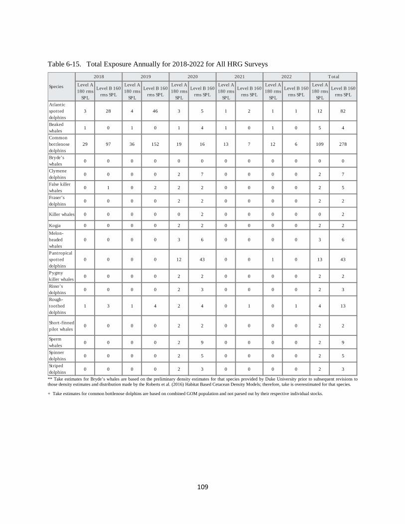
109

Table 6-15. Total Exposure Annually for 2018-2022 for All HRG Surveys

** Take estimates for Bryde’s whales are based on the preliminary density estimates for that species provided by Duke University prior to subsequent revisions to those density estimates and distribution made by the Roberts et al. (2016) Habitat Based Cetacean Density Models; therefore, take is overestimated for that species. + Take estimates for common bottlenose dolphins are based on combined GOM population and not parsed out by their respective individual stocks.

Level A 180 rms

SPL

Level B 160 rms SPL

Level A 180 rms

SPL

Level B 160 rms SPL

Level A 180 rms

SPL

Level B 160 rms SPL

Level A 180 rms

SPL

Level B 160 rms SPL

Level A 180 rms

SPL

Level B 160 rms SPL

Level A 180 rms

SPL

Level B 160 rms SPL

Atlantic spotted dolphins

3 28 4 46 3 5 1 2 1 1 12 82

Beaked whales 1 0 1 0 1 4 1 0 1 0 5 4

Common bottlenose dolphins

29 97 36 152 19 16 13 7 12 6 109 278

Bryde’s whales 0 0 0 0 0 0 0 0 0 0 0 0

Clymene dolphins 0 0 0 0 2 7 0 0 0 0 2 7

False killer whales 0 1 0 2 2 2 0 0 0 0 2 5

Fraser’s dolphins 0 0 0 0 2 2 0 0 0 0 2 2

Killer whales 0 0 0 0 0 2 0 0 0 0 0 2

Kogia 0 0 0 0 2 2 0 0 0 0 2 2Melon-headed whales

0 0 0 0 3 6 0 0 0 0 3 6

Pantropical spotted dolphins

0 0 0 0 12 43 0 0 1 0 13 43

Pygmy killer whales 0 0 0 0 2 2 0 0 0 0 2 2

Risso’s dolphins 0 0 0 0 2 3 0 0 0 0 2 3

Rough-toothed dolphins

1 3 1 4 2 4 0 1 0 1 4 13

Short-finned pilot whales

0 0 0 0 2 2 0 0 0 0 2 2

Sperm whales 0 0 0 0 2 9 0 0 0 0 2 9

Spinner dolphins 0 0 0 0 2 5 0 0 0 0 2 5

Striped dolphins 0 0 0 0 2 3 0 0 0 0 2 3

Total

Species

2018 2019 2020 2021 2022

110

Table 6-16. Estimate Level A and Level B Exposures Estimates for All Analyzed Gulf of Mexico Species per Survey Types (unmitigated) for 2018-2022

Survey Type

2018 2019 2020 2021 2022 Total

Level A 180 rms SPL

Level B 160 rms

SPL

Level A 180 rms SPL

Level B 160 rms

SPL

Level A 180 rms SPL

Level B 160 rms

SPL

Level A 180 rms SPL

Level B 160 rms

SPL

Level A 180 rms SPL

Level B 160 rms

SPL

Level A 180 rms

SPL

Level B 160 rms

SPL

2-D 0 0 7269 188532 0 0 0 0 4908 127268 12177 315800

3-D NAZ 293660 1940265 407956 2088750 292456 1878136 401891 2217956 296284 1736778 1692247 9861885

3-D WAZ 42401 544927 72452 494103 44896 567663 88261 707223 41558 521029 289568 2834945

Coil 18035 114863 21477 93034 19025 120826 28224 139015 17626 109157 104387 576895

HRG 18 118 19 128 23 63 0 0 0 0 60 309

Boomer 0 0 9 66 20 43 0 0 0 0 29 109

Side-scan sonar, sub-bottom profiler, and multibeam scanner

16 11 14 10 17 11 15 10 15 8 77 50

Total 2098545 13589993

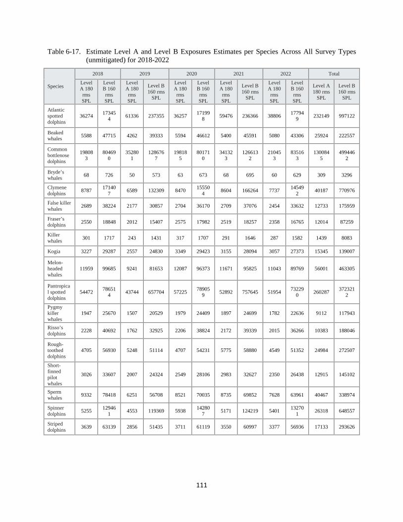
111

Table 6-17. Estimate Level A and Level B Exposures Estimates per Species Across All Survey Types (unmitigated) for 2018-2022

Species

2018 2019 2020 2021 2022 Total

Level A 180 rms SPL

Level B 160 rms SPL

Level A 180 rms SPL

Level B 160 rms

SPL

Level A 180 rms SPL

Level B 160 rms SPL

Level A 180 rms SPL

Level B 160 rms

SPL

Level A 180 rms SPL

Level B 160 rms SPL

Level A 180 rms

SPL

Level B 160 rms

SPL

Atlantic spotted dolphins

36274 173454 61336 237355 36257 17199

8 59476 236366 38806 177949 232149 997122

Beaked whales 5588 47715 4262 39333 5594 46612 5400 45591 5080 43306 25924 222557

Common bottlenose dolphins

198083

804690

352801

1286767

198185

801710

341323

1266132

210453

835163

1300845

4994462

Bryde’s whales 68 726 50 573 63 673 68 695 60 629 309 3296

Clymene dolphins 8787 17140

7 6589 132309 8470 155504 8604 166264 7737 14549

2 40187 770976

False killer whales 2689 38224 2177 30857 2704 36170 2709 37076 2454 33632 12733 175959

Fraser’s dolphins 2550 18848 2012 15407 2575 17982 2519 18257 2358 16765 12014 87259

Killer whales 301 1717 243 1431 317 1707 291 1646 287 1582 1439 8083

Kogia 3227 29287 2557 24830 3349 29423 3155 28094 3057 27373 15345 139007

Melon-headed whales

11959 99685 9241 81653 12087 96373 11671 95825 11043 89769 56001 463305

Pantropical spotted dolphins

54472 786514 43744 657704 57225 78905

9 52892 757645 51954 732290 260287 372321

2

Pygmy killer whales

1947 25670 1507 20529 1979 24409 1897 24699 1782 22636 9112 117943

Risso’s dolphins 2228 40692 1762 32925 2206 38824 2172 39339 2015 36266 10383 188046

Rough-toothed dolphins

4705 56930 5248 51114 4707 54231 5775 58880 4549 51352 24984 272507

Short-finned pilot whales

3026 33607 2007 24324 2549 28106 2983 32627 2350 26438 12915 145102

Sperm whales 9332 78418 6251 56708 8521 70035 8735 69852 7628 63961 40467 338974

Spinner dolphins 5255 12946

1 4553 119369 5938 142807 5171 124219 5401 13270

1 26318 648557

Striped dolphins 3639 63139 2856 51435 3711 61119 3550 60997 3377 56936 17133 293626

112

Table 6-18. Estimate Level A and Level B Exposures Estimates Including Updated NMFS Criteria per Species Across All Survey Types (unmitigated) for 2018-2022

Species Number of Level A Exposures Number of Level B Exposures

peak SPL SEL 180 rms SPL Step fxn 160 rms SPL Atlantic spotted dolphins 1,723.1 154.9 232,139.0 702,746.5 997,109.1 Beaked whales 218.1 10.4 25,910.2 914,325.0 222,549.6 Common bottlenose dolphins 11,059.7 583.4 1,300,832.3 3,752,256.7 4,994,450.8 Bryde’s whales 1.5 60.4 300.3 2,793.0 3,288.2 Clymene dolphins 1.693.0 126.6 40,180.2 424,852.4 770,967.3 False killer whales 446.9 40.6 12,723.9 99,934.7 175,948.4 Fraser’s dolphins 207.1 11.7 12,003.6 54,510.5 87,250.6 Killer whales 19.6 2.0 1,433.4 5,858.6 8,073.1 Kogia 17,701.8 2,201.3 15,335.4 64,151.2 138,998.5 Melon-headed whales 1,000.2 59.4 55,990.4 270,012.1 463,296.0 Pantropical spotted dolphins 10,227.9 506.3 260,276.1 2,379,386.7 3,723,203.8 Pygmy killer whales 333.4 28.4 9,101.7 70,227.8 117,935.6 Risso’s dolphins 436.6 56.3 10,374.2 104,423.1 188,038.4 Rough-toothed dolphins 628.2 58.8 24,973.7 156,663.1 272,492.4 Short-finned pilot whales 259.6 26.9 12,903.9 72,658.2 145,092.1 Sperm whales 175.0 8.7 40,457.3 161,660.2 338,966.8 Spinner dolphins 1,060.3 39.8 26,310.6 330,013.8 648,549.2 Striped dolphins 694.4 41.3 17,123.8 171,317.4 293,617.0

113

7 ANTICIPATED IMPACT OF THE ACTIVITY TO THE SPECIES OR STOCK OF MARINE MAMMAL

Anticipated Level A and Level B impacts of the proposed activities to the species or stock of marine mammals are discussed in Section 6. Again, exposure of an animal to a sound is not necessarily equivalent to the animal being taken. Instead, there are many factors that influence whether an individual animal will be harassed (“taken”) from an exposure, such as age, individual hearing capability, prior experience with the same noise, and behavior during exposure. At the same time, there are no currently available robust, quantitative measures to translate exposures to takes, especially at the broader programmatic and aggregate scale that is the subject of this petition. In lieu of such a method, the exposure numbers in Section 6 should be considered as precautionary estimates of potential exposures, including repeated exposures of the same individual to sound levels exceeding NMFS’ acoustic criteria levels.

The section provides narrative context to help more qualitatively interpret the potential range of effects from the modeled exposures. It first focuses on the underlying acoustic criteria used to estimate exposures. It then discusses the types of effects that may occur from these exposures (e.g., hearing threshold shifts (injury), stress and behavioral response, masking, impacts to prey species). Finally, it looks at the potential for types of impacts per sound source category (airguns and electromechanical sources).

7.1 ACOUSTIC EXPOSURE CRITERIA Underlying the assessment of potential impacts to marine mammals is the understanding and

application of acoustic exposure criteria for marine mammals. Since the mid-1990s, the USDOC, NMFS (2003) has specified that cetaceans exposed to pulsed sounds with received SPLs exceeding 180 dB re 1 μPa (rms) would be considered as potentially injured under the MMPA and experience Level A harassment. The NMFS also considers that marine mammals exposed to pulsed sound levels >160 dB re 1 μPa (rms) are subject to MMPA Level B harassment.

In addition to the NMFS historic criteria, the analysis underlying this petition also considers acoustic energy for MMPA Level B harassment using the Wood et al. (2012) methodology and MMPA Level A using the Southall et al. (2007) methodology. More details on the acoustic exposure criteria are provided in Appendix B. Both the Wood et al. (2012) and Southall et al. (2007) methods include frequency weighting to account for animal hearing sensitivities. Sound is less likely to injure or disturb animals if it occurs at frequencies to which the animal is less sensitive. Based on a review of marine mammal hearing and on physiological and behavioral responses to anthropogenic sound, three functional hearing groups of cetaceans (Table 7.2) have been defined (Southall et al., 2007; Finneran and Jenkins, 2012):

● low-frequency cetaceans (mysticetes);

● mid-frequency cetaceans (some odontocetes); and

● high-frequency cetaceans (some odontocetes).

Of the marine mammal species occurring in the GOM, the Bryde’s whale is the only low-frequency cetacean and Kogia species (i.e., the dwarf sperm whale and pygmy sperm whale) are

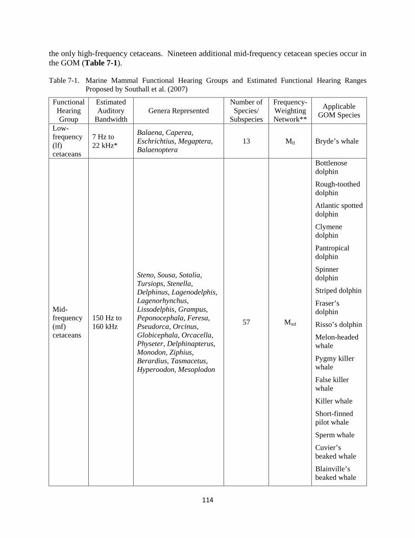
114

the only high-frequency cetaceans. Nineteen additional mid-frequency cetacean species occur in the GOM (Table 7-1).

Table 7-1. Marine Mammal Functional Hearing Groups and Estimated Functional Hearing Ranges

Proposed by Southall et al. (2007)

Functional Hearing Group

Estimated Auditory

Bandwidth Genera Represented

Number of Species/

Subspecies

Frequency-Weighting Network**

Applicable GOM Species

Low-frequency (lf) cetaceans

7 Hz to 22 kHz*

Balaena, Caperea, Eschrichtius, Megaptera, Balaenoptera

13 Mlf Bryde’s whale

Mid-frequency (mf) cetaceans

150 Hz to 160 kHz

Steno, Sousa, Sotalia, Tursiops, Stenella, Delphinus, Lagenodelphis, Lagenorhynchus, Lissodelphis, Grampus, Peponocephala, Feresa, Pseudorca, Orcinus, Globicephala, Orcacella, Physeter, Delphinapterus, Monodon, Ziphius, Berardius, Tasmacetus, Hyperoodon, Mesoplodon

57 Mmf

Bottlenose dolphin

Rough-toothed dolphin

Atlantic spotted dolphin

Clymene dolphin

Pantropical dolphin

Spinner dolphin

Striped dolphin

Fraser’s dolphin

Risso’s dolphin

Melon-headed whale

Pygmy killer whale

False killer whale

Killer whale

Short-finned pilot whale

Sperm whale

Cuvier’s beaked whale

Blainville’s beaked whale

115

Gervais’ beaked whale

High-frequency (hf) cetaceans

200 Hz to 180 kHz

Phocoena, Neophocaena, Phocoenoides, Platanista, Inia, Kogia, Lipotes, Pontoporia, Cephalorhynchus

19 Mhf Dwarf and pygmy sperm whale

*As described in the text, more recent modeling work would suggest that the upper frequency end of the estimated auditory bandwidth may be slightly higher (approximately 30 kHz), at least for some species.

**Southall et al., 2007.

Southall et al. (2007) defined Type I M-weighting functions for each functional hearing group, which is used in the MMPA Level B criteria of Wood et al. (2012). The Southall et al. (2007) Type I M-weighting was updated for MMPA Level A impacts for low-, mid-, and high-frequency cetaceans by Finneran and Jenkins (2012), termed Type II weighting. Because limited data exist for low-frequency cetaceans, the Type I M-weighting is used here with the Southall et al. (2007) Level A criteria, whereas the Type II weighting, updated with the best available research conducted since Southall et al. (2007) was published, is used for mid- and high-frequency cetaceans (Finneran and Jenkins, 2012).

The Wood et al. (2012) Level B criteria use a graded step function to acknowledge that most marine mammals exhibit varying responses between SPLrms of 140 dB and 180 dB re 1 μPa. For pulsed sounds, a graded probability of response with 10 percent response likelihood at an rms of 140 dB re 1 μPa, 50 percent at an SPLrms of 160 dB re 1 μPa, and 90 percent at an SPLrms of 180 dB 1 μPa was used for all species except beaked whales. Sensitive species, such as beaked whales, exhibit the likelihood of a 50 percent response at an SPLrms of 120 dB re 1 μPa and a 90 percent response at an SPLrms of 140 dB re 1 μPa (Wood et al., 2012; Appendix B, Table 6).

The Southall et al. (2007) Level A criteria acknowledge that there two mechanisms for an animal to experience Level A exposures, fatiguing of the sensory system measured with a cumulative sound exposure level (SEL) threshold and tissue damage measured with a peak SPL threshold. The SEL criteria are frequency weighted (Type I M-weighting for Bryde’s whale; Type II weighting for all other species) and are 192, 187, and 161 dB re 1 µPa2·second, respectively, for low-, mid-, and high-frequency cetaceans. The peak SPL criteria are not weighted and are 230 dBpeak re 1 µPa for low- and mid-frequency cetaceans and 200 dBpeak re 1 µPa for high-frequency cetaceans (Southall et al., 2007; Appendix B, Table 5).

Therefore, there are two criteria used for Level B harassment: the traditional NMFS criteria (160 dB rms) and the step function of Wood et al. (2012). There are two criteria used for Level A harassment: the traditional NMFS criteria (180 dB rms) and the SEL and SPLpeak criteria of Southall et al. (2007).

As previously noted, NMFS provided updated Level A criteria in July 2016 based on the advances in the understanding of the impacts of noise on marine mammals. BOEM does anticipate, however, that the July 2016 changes to NMFS’ acoustic criteria likely mean the Level A exposures predicted in the modeling used for the Draft PEIS and this petition are, in most cases, overestimates.

7.2 POTENTIAL TYPES OF EFFECTS OF NOISE ON MARINE MAMMALS This petition requests take authorization for Level A and Level B (primarily) harassment

from exposure to acoustic sound sources. It does not request mortality given there is no evidence

116

or belief that mortality will occur from the proposed action, especially with the required mitigation and monitoring.

Overall, the potential for noise impacts from these sound sources on marine mammals is highly variable and depends on the specific circumstances of a given situation. Furthermore, the same sound source can propagate differently depending on the physical environment. The sections to following provide a baseline as well as BOEM’s conclusions on the potential effects of impacts from these sound sources, including auditory injuries, masking, stress, behavioral disruption and effects on prey species.

7.2.1 Auditory Injuries – Threshold Shift Physical impacts to an animal’s auditory system can occur from exposure to intense sounds

and can result in the animal losing hearing sensitivity. A temporary threshold shift (TTS) is hearing loss that persists only for minutes or hours, whereas a permanent threshold shift (PTS) is indefinite. The severity of TTS is expressed as the duration of hearing impairment (lowered sensitivity in the bandwidths in which the noise was centered) and the magnitude of the shift in hearing sensitivity relative to pre-exposure sensitivity. The TTS generally occurs at lower sound levels than PTS. Repeated TTS, especially if the animal is receiving another loud sound exposure before recovering from the previous TTS, is thought to cause PTS (Lin et al. 2011). If the sound is intense enough, however, an animal can succumb to PTS without first experiencing TTS (Weilgart 2007). Though the relationship between the onset of TTS and the onset of PTS is not fully understood, TTS onset is used to predict sound levels that are likely to result in PTS. Further, sound level and duration are key determinants in TTS. The SEL metric includes amplitude, duration, and TTS magnitude (refer to Appendix B for more detail on assumptions used in modeling for Level A [e.g., onset of TTS] exposures).

At present, there are multiple existing criteria available for predicting the onset of TTS and subsequently PTS. In July 2016, NOAA/NMFS released the final version of “The Technical Guidance for Assessing the Effects of Anthropogenic Sound on Marine Mammal Hearing.” This document provided acoustic guidelines (specifically those that identify the onset of PTS or TTS) to be used when conducting impact analyses for marine mammals. As NMFS stated in their Executive Summary, “While the Technical Guidance’s acoustic thresholds are more complex than those used to date in most cases by NMFS, they reflect the current state of the scientific knowledge regarding the characterization of sound that have the potential to impact marine mammal hearing sensitivity.” Throughout the development of this new guidance, BOEM provided comment and review.

Before this final version was complete and in July 2015, BOEM completed modeling efforts to assess the potential acoustic impacts from G&G activities for use in the GOM PEIS (refer to Appendix B). These modeling efforts used the acoustic guidance that was available from NMFS at that time which specified that marine mammals exposed to pulsed sounds with received levels exceeding 180 or 190 decibels referenced to 1 μPa (rms) (dB re 1 μPa [rms]) are considered to exceed Level A (Injury) levels. The NMFS also specified at that time that cetaceans exposed to levels exceeding 160 dB re 1 μPa (rms) are considered to exceed Level B (Behavioral Harassment) criteria. Both Southall et al. (2007) and NOAA’s first and second draft underwater acoustic guidances (USDOC, NOAA, 2013, 2015) delineated new acoustic threshold levels for the onset of PTS and TTS. They also recommended the use of the dual criteria metrics of SEL (specifically, cumulative SEL [SELcum]) and peak SPL (SPLpeak) as most appropriate for establishing the onset levels for TTS and PTS in marine mammals (USDOC, NOAA, 2013,

117

2015). The SPLpeak threshold would be applied to unweighted (unfiltered) sound levels, while the SELcum metric would be calculated using M-weighting. Thus, any received noise that exceeds the SPLpeak or SELcum criterion for injury is assumed to cause tissue injury in an exposed marine mammal. It is worthwhile to note that this application of the SELcum approach does not include the possibility of recovery of hearing between repeated exposures. Table 7-2 provides a comparison of the levels provided in Southall et al. (2007) and USDOC, NOAA (2013, 2015).

Table 7-2. Dual Injury Criteria for Marine Mammals Exposed to Impulsive Noise Over a 24-Hour

Period (From: Southall et al., 2007; USDOC, NOAA, 2015, 2013)

Marine Mammal Hearing Group

TTS Onset PTS Onset Southall et al.

(2007) USDOC, NOAA

(2013) Southall et al.

(2007) USDOC, NOAA

(2015) SPLpeak

1 SELcum

2 SPLpeak

1 SELcum

2 SPLpeak

1 SELcum

2 SPLpeak

1 SELcum

2 Low-frequency cetaceans 224 183 224 172 230 198 230 192

Mid-frequency cetaceans 224 183 224 172 230 198 230 187

High-frequency cetaceans 224 183 195 146 230 198 202 154

NOAA = National Oceanic and Atmospheric Administration; PTS = permanent threshold shift; SELcum = cumulative sound exposure level; SPLpeak = peak sound pressure level; TTS = temporary threshold shift. 1 Measured in dB re 1 µPa. 2 Measured in dB re 1 µPa2•s.

At the time that the potential impact calculations were made for this petition, these SELcum criteria were not yet available (they had not been published or officially released); therefore, the best available estimate of these values were 192 dB, 187 dB, and 161 dB, respectively, for low-, mid-, and high-frequency cetaceans (Appendix B). The current NOAA regulatory thresholds, however, are based on SPLrms metrics (i.e., 180 dB re 1 μPa [rms] for injury; 160 dB re 1 μPa [rms] for behavioral disturbance); the SPLrms metrics cannot be directly compared with the SPLpeak metrics. However, the analysis in Appendix B also includes the stepped threshold function that was developed and presented in Finneran and Jenkins (2012) and Wood et al. (2012). Further discussion of the current noise exposure thresholds is provided in a previous section titled “Acoustic Exposure Criteria.”

Conclusion: Auditory Injuries –Threshold Shift

Table 7-3 below captures all of the Level A exposures predicted through the acoustic modeling done to support this petition (refer to Appendix B). Summarizing these Level A exposures in one table helps identify which types of activities have a low potential for Level A exposures and where high potential might exist (albeit still largely unmitigated). Table 7-4 presents the estimated number of Level A exposures for species with all survey types.

118

Table 7-3. Estimated Level A Exposures for Different Survey Types (unmitigated) Using the GOM G&G Scenario for 2018-2022

Table 7-4. Estimate Level A Exposures per Species for Five Years and Across All Survey Types (unmitigated)

Species Number of Level A exposures

peak SPL SEL 180 rms SPL Atlantic spotted dolphins 302.4 30.4 38,803.6 Beaked whales 41.9 1.7 5076.4 Common bottlenose dolphins 1,890.0 134.3 210,451.4 Bryde’s whales 0.3 11.2 57.0 Clymene dolphins 315.9 20.6 7,735.4 False killer whales 84.5 6.9 2,452.5 Fraser’s dolphins 39.0 1.9 2,355.5 Killer whales 3.8 0.4 285.9 Kogia 3,585.0 419.9 3,054.8 Melon-headed whales 188.9 9.8 11,040.9 Pantropical spotted dolphins 1,998.7 93.2 51,950.6 Pygmy killer whales 63.5 4.9 1,780.6 Risso’s dolphins 83.6 10.3 2,012.3 Rough-toothed dolphins 117.1 10.1 4,547.2 Short-finned pilot whales 46.0 4.1 2,347.1 Sperm whales 33.6 1.5 7,627.1 Spinner dolphins 212.0 8.0 5,399.8 Striped dolphins 133.3 7.2 3,375.6

119

Sound sources used during geophysical activities produce sound levels sufficient to cause TTS or PTS in marine mammals without appropriate mitigation measures. For PTS, the animal would need to be in very close range (meters) of the source. The TTS could occur at slightly further distances from the source. Section 11 outlines the mitigation and monitoring measures that will be required. Central to the issue of PTS and TTS is the establishment of exclusion zones around the sources, visual and acoustic monitoring of these zones by trained observers, restrictions on starting sound sources until after the zone is cleared of marine mammals and, in designated instances, the shut down of the sound source should an animal be observed within or approaching the zone. Collectively, these measures decrease the potential for marine mammals to be in close proximity of the sound source, thereby avoiding the highest sound levels and the potential for TTS or PTS. This is, however, not a guarantee, and BOEM has included some Level A Harassment take requests within this petition (refer to Tables 6-14 and 6-15 in Section 6).

7.2.2 Auditory Masking Noise can partially or completely reduce an individual’s ability to effectively communicate;

detect important predator, prey, and conspecific signals; and detect important environmental features associated with spatial orientation (Clark et al., 2009). Increases in ambient noise levels can result in auditory masking, which is the reduction in the detectability of a sound signal of interest (e.g., communication calls and echolocation) due to the presence of another sound, which is usually noise in the environment and often is at a similar frequency. Under normal circumstances, in the absence of high ambient noise levels, an animal would hear a sound signal because it is above its absolute hearing threshold. Auditory masking prevents part or all of a sound signal from being heard and decreases the distances that underwater sound can be detected by marine animals (i.e., reduction in communication space). This may have no impact on an animal or may cause a long-term decrease in a marine mammal’s efficiency at foraging, navigating, or communicating (International Council for the Exploration of the Sea, 2005). For some types of marine mammals, specifically bottlenose dolphins, beluga whales, and killer whales, empirical evidence confirms that the degree of masking depends strongly on the relative directions at which sound arrives and the characteristics of the masking noise (Penner et al., 1986; Dubrovskiy, 1990; Bain et al., 1993; Bain and Dahlheim, 1994).

Ambient noise from natural and anthropogenic sources can cause masking in marine animals, effectively interfering with the ability of an animal to detect a sound signal that it otherwise would hear. Spectral, temporal, and spatial overlap between the masking noise and the sender/receiver determines the extent of interference; the greater the spectral and temporal overlap, the greater the potential for masking. Naturally occurring ambient noise is produced from various sources, including environmental sounds from wind, waves, precipitation, earthquakes; biological sounds produced by animals; and thermal noise resulting from molecular agitation (at frequencies above 30 kHz) (Richardson et al., 1995). Marine biota produce sounds that contribute to the ambient noise environment. Fish, for example, create low-frequency sounds (50 to 2,000 Hz, most often from 100 to 500 Hz) that can be a significant component of local ambient sound levels (Zelick and Mann, 1999). Ambient noise also can be generated by anthropogenic sources such as boats and ships, sonars (military and commercial), geophysical exploration, acoustic deterrent devices, construction noise, and scientific research sensors.

120

Ambient noise is highly variable in the shallower waters over continental shelves (Desharnais et al., 1999) where many anthropogenic activities occur; effectively creating a high degree of variability in the range at which marine mammals can detect anthropogenic sounds. In coastal waters, noise from boats and ships, particularly commercial vessels, are the predominant source of anthropogenic noise (Parks et al., 2011). Snyder and Orlin (2007) noted that shipping noise dominated the low frequencies (25 to 400 Hz) of the ambient underwater noise environment of the GOM.

Over the past 50 years, commercial shipping, the largest contributor of masking noise (McDonald et al., 2008), has increased the ambient sound levels in the deep ocean at low frequencies by 10 to 15 dB (Hatch and Wright, 2007). This increase in low-frequency ambient noise coincides with a significant increase in the number and size of vessels making up the world’s commercial shipping fleet (Hildebrand, 2009). Tournadre (2014) estimated from satellite altimetry data that, globally, ship traffic grew by approximately 60 percent from 1992 to 2002, at a nearly constant rate of approximately 6 percent per year; however, after 2002, the rate at which shipping increased rose steadily to >10 percent by 2011, except in 2008 to 2009, when ship traffic remained steady. Globally, Tournadre (2014) estimated that shipping between 1992 and 2011 grew by a factor of four, with the highest growth in the Indian and western North Pacific Oceans, especially in the continental seas along China; growth in shipping in the Atlantic Ocean and Mediterranean Sea, however, decreased after 2008. Aguilar-Soto et al. (2006) reported that the noise from a passing vessel masked ultrasonic vocalizations of a Cuvier’s beaked whale and reduced the maximum communication range by 82 percent when exposed to a 15-dB increase in ambient sound levels at the vocalization frequencies; the effective detection distance of the Cuvier’s beaked whale’s echolocation clicks was reduced by 58 percent. Low-frequency noise (20 to 200 Hz) from large ships overlaps the frequency range of acoustic vocalizations of some mysticetes, and increased levels of underwater noise have been documented in areas with high shipping traffic, causing responses in some mysticetes that have included habitat displacement; changes in behavior; and alterations in the intensity, frequency, and intervals of their calls (Rolland et al., 2012).

Marine mammals are able to compensate, to a limited extent, for auditory masking through a variety of mechanisms, including increasing source levels (Lombard effect) or durations of their vocalizations or by changing spectral and temporal properties of their vocalizations (Parks et al., 2010; Hotchkin and Parks, 2013). In the presence of ship noise, beluga whales produced whistles of higher frequency and longer duration (Lesage et al., 1999). Di Iorio and Clark (2010) found that blue whales increased their rate of social calling in the presence of seismic exploration sparkers (plasma sound sources), which presumably represented a compensatory behavior to elevated ambient noise levels from seismic surveys. Bowhead whales were found to increase their calling rate in response to seismic airgun signals at low levels (approximately 94 dB re 1µPa2-s, CSEL; integrated over 10 minutes). However, when those signals exceeded approximately 127 dB CSEL, their calling rate began to decrease, and when it reached approximately 160 dB CSEL, the bowheads stopped calling completely (Blackwell et al., 2015). Note that these received levels were measured at a recorder within 2 km (1 mi) of the whales; therefore, the received levels at the whales are approximations. These examples of baleen whale responses to sound are informative, even though these species are not found in the GOM. Several marine mammal species are known to increase the source levels of their calls in the presence of elevated sound levels (Dahlheim, 1987; Au, 1993; Lesage et al., 1999; Terhune, 1999; Holt et al., 2009; Melcón et al., 2012). Holt et al. (2009) studied the effects of anthropogenic sound

121

exposure on the endangered southern resident killer whales in Puget Sound, reporting that these whales increased their call amplitude by 1 dB SPL for every 1 dB SPL increase in background noise (1 to 40 kHz). Castellote et al. (2012) hypothesized that the fin whales modified their acoustic communications to compensate for the increased background noise and that the animals had a lower tolerance for seismic airgun noise than for shipping noise, perhaps having become desensitized to the ambient shipping noise. Melcón et al. (2012) found that blue whales stopped calling in the presence of mid-frequency active sonar transmissions and conversely increased their vocalization rate when the sonar was transmitting.

Conclusion: Auditory Masking

Southall et al. (2007) considered auditory masking issues and realized the much greater relative areas over which this phenomena could occur relative to TTS and PTS, but they did not propose explicit exposure criteria for marine mammals, owing in part to the very divergent conditions in which masking can occur and a lack of clear understanding about defining an “onset” for masking that would be statistically definable and biologically meaningful. Largely for the same reasons, masking effects generally have been considered only qualitatively in planning of activities and regulatory decisions related to noise impacts.

Effective detection of sounds is critical for aquatic animals and methods are needed to assess and minimize the longer-term and aggregate effects of noise on marine species and their habitat, in addition to acute impacts at closer range. NMFS conducted a first-order assessment of the chronic and cumulative effects of noise produced by seismic activities in the GOM. Modeling was conducted for 10 locations of biological importance and for four scenarios corresponding to G&G survey alternatives found in the Draft Gulf of Mexico G&G Programmatic EIS. These include full proposed levels of seismic, 25 percent reduction in seismic, and both with and without time/area closures at each of these activity levels (Alternatives C, E, F1 and F2, as described in the Draft Gulf of Mexico G&G Programmatic EIS; USDOI, BOEM, 2016). “Lost listening area” was calculated among each of the four scenarios and relative to a baseline ambient noise estimate, for the full modeled frequency bandwidth (10-5000 Hz), and adjusted to account for the hearing sensitivity of low, mid-, and high frequency cetaceans.

While there is ample evidence to support the fact that significant reductions in listening area or communication space can negatively affect aquatic animals, data is lacking to document links to consequences for long-lived and often wide-ranging species such as marine mammals. In contrast with estimation of acoustic harassment, NMFS’ chronic and cumulative effects analysis was not designed to evaluate the exposure of individual animals to seismic sources from one moment to the next. Rather, the analysis was intended to ensure consideration of the longer-term and wider-ranging noise effects from these sources and to augment the more traditional analysis of acute effects (occurrence of exposure that may potentially cause injury and behavioral harassment) addressed in Chapter 4 of the GOM G&G Draft PEIS (BOEM 2016).

While these results are broadly informative (especially when considered as a whole across the GOM), it is important to remain cognizant of the methods and simplifying assumptions when making location-specific interpretations and comparisons. For example, the distribution in space and time of seismic survey activity will significantly influence the resulting cumulative noise exposure at a specific location. Here, projected levels are distributed uniformly within planning areas, but actualized survey activity may result in higher concentrations in some areas within the planning areas and lower concentrations in others. The effect of concentrations of activity in high proximity to selected locations will continue to be offset by the methods applied here to

122

remove the closest 10 percent of pulses in order to focus on long-term accumulation of energy at regional scales. However, this same method can result in an under-representation of the value of closure areas at maintaining listening and communication space. Similarly, the assumption made here that 25 percent of the activity that would have occurred in a closure area would be redistributed outside that area must be carefully considered when interpreting results as this consequence is yet unknown (i.e., applying closures results in increased levels of activity in remaining area outside of closures).

All of the listening area losses are relativistic, and most examine the differences in areas available under different seismic activity scenarios, without reliance on the difficult task of evaluating levels of noise in the absence of seismic in the GOM.

Sound sources used during geophysical survey activities could mask marine mammal communication and monitoring of the environment around them if the hearing sensitivities of the marine mammals present coincide with the frequency of the sound source being used. As airgun signals propagate away from the source, their amplitude drops, which reduces their masking effect. However, the multipath effects of propagation increase the duration of the signals, which increases the proportion of time that they can potentially mask animal signals. Survey protocols and underwater noise mitigation procedures, particularly shutdowns that are designed to reduce the PTS, may also decrease the potential risk for any marine mammal to experience auditory masking because the source would not operate when animals are close.

Lastly, BOEM points to the development of a novel analytical method to evaluate the effects of human noise on marine mammal hearing and behavior which may provide additional insight and information on masking and possible details about “lost listening space” and what that means biologically/physiologically to marine mammals. A research collaboration of world-leading scientists1 in underwater sound, marine mammal hearing and behavior recently produced an acoustic Risk Assessment Framework (RAF). In broad terms, the acoustic RAF considers the results of conventional assessments (e.g., exposure estimates) and, through a rigorous analytical methodology, interprets what these estimates mean within the context of key biological and population parameters (e.g., population size, life history factors, compensatory ability of the species, animal behavioral state, source-animal proximity, relative motion, variance in density estimates, aversion) as well as other biological, environmental, and anthropogenic factors. The end result provides not just numbers of exposures, which is what conventional approaches to modeling provides, but instead what these numbers mean biologically for each affected marine mammal stock/population (severity of impact, vulnerability of stock/population) as well as the likelihood of any such impact.

7.2.3 Stress and Behavioral Responses Stress and behavioral changes are the result of marine mammals responding to extreme or

excessive disturbances in their environment, either of natural or anthropogenic origin. Stress responses typically are physiological changes in a marine mammal’s blood chemistry while behavioral responses involve changes in a marine mammal’s normal actions.

Stress is a change in the body’s equilibrium in response to an extreme environmental or physiological disruption. Marine mammals respond to environmental stress by releasing 1 Dr. Brandon Southall, Southall Environmental Associates Dr. Bill Ellison, Marine Acoustics, Inc. Dr. Chris Clark, Marine Acoustics, Inc. Dr. Dominic Tollit, SMRU Consulting

123

biochemicals into their blood streams. The NRC (2003) discussed acoustically induced stress in marine mammals, stating that one-time exposures to sound are less likely to have population-level effects than sounds that animals are exposed to repeatedly over extended periods of time. Various researchers have summarized the available evidence regarding stress-induced events. Romano et al. (2004) exposed a beluga whale to varying levels of an impulsive signal and measured the levels of three stress-related blood hormones after control, low-level sound (171 to 181 dB SEL), and high-level sound (184 to 187 dB SEL) exposure; no significant differences in the hormone blood concentrations were found between the control and low-level sound exposure, but elevated levels of all three hormones were produced in response to high-level sound exposure. Furthermore, regression analysis demonstrated a linear trend for increased hormone level with sound level. Rolland et al. (2012) showed that a 6-dB decrease in the ambient underwater noise level, including a significant reduction below 150 Hz, was associated with decreased baseline levels of stress-related hormone metabolites in whales. This reduction in ambient noise levels associated with shipping was the first evidence that exposure to low-frequency noise from shipping may be associated with chronic stress in whales (Rolland et al., 2012).

Behavioral responses, including startle, avoidance, displacement, diving, and vocalization alterations, have been observed in mysticetes, odontocetes, and pinnipeds and in some cases; these have occurred at ranges of tens to hundreds of kilometers from the sound source (Gordon et al., 2004; Tyack, 2008; Miller et al., 2014). However, behavioral observations are variable, some findings contradictory, and the biological significance of the effects has not been measured (Gordon et al., 2004). Behavioral reactions of marine mammals to sound are difficult to predict because reactions depend on numerous factors including the species being evaluated; the animal’s state of maturity, prior experience and exposure to anthropogenic sounds, current activity patterns, and reproductive state; time of day; weather state; the potential for individual differences within species; and different species reacting differently to the same sounds (Nowacek et al., 2004; Wartzok et al., 2004; Bain and Williams, 2006; Castellote et al., 2014). The severity of responses can vary depending on characteristics of the sound source (e.g., moving or stationary, number and spatial distribution of sound source[s], similarity to predator sounds, and other relevant factors) (Richardson et al., 1995; NRC, 2005; Southall et al., 2007; Bejder et al., 2009; Barber et al., 2010; Ellison et al., 2011). If a marine mammal reacts to an underwater sound by changing its behavior or moving to avoid a sound source, the impacts of that change may not be important to the individual, stock, or species as a whole. However, if a sound source displaces marine mammals from an important feeding or breeding area, impacts on individuals and the population could be important.

Acoustic reactions of cetaceans to airgun activity may include increased and/or reduced vocalization rates (Goold, 1996; Blackwell et al., 2015), no vocal changes (Madsen et al., 2002), or cessation of singing (McDonald et al., 1995). Other short-term vocal adjustments observed across species exposed to elevated ambient noise levels include shifting call frequency, increasing call amplitude or duration, and ceasing to call (Nowacek et al., 2007). Di Iorio and Clark (2010) suggested, later supported by Ellison et al. (2012), the exposure context of the received seismic sparker sound strongly influenced the probability and type of behavioral response in blue whales. Acoustic and behavioral changes by fin whales in response to shipping and airgun noise found that the acoustic features of fin whale 20-Hz song notes were affected in high-noise conditions (Castellote et al., 2012). Studies on humpback whales reported their avoidance of seismic surveys (McCauley et al., 2000).

124

Few dedicated studies of the behavioral responses of GOM marine mammals have been conducted, especially to seismic activities. Mate et al. (1994) noted that sperm whales were displaced in the northern GOM off the Louisiana coast following seismic surveys in the area. Sperm whale sightings through Protected Species Observer reports during seismic surveys in the GOM showed a significant difference in the closest point of approach distance between times of airgun silence and full power, with greater distances from the source displayed during full power (Barkaszi et al 2012). Miller et al. (2009) reported the lack of a behavioral response in eight tagged sperm whales in the GOM that were exposed to received levels of 111-147 dB rms from a large airgun array. However, Miller et al. (2009) suggested that, while the surface observations were indicative of no behavioral disruption, the lower pitch and buzz rates the tags recorded while the sperm whales were exposed to the airgun noise may have been indicative of impacts to feeding rates.

There is significant species-specific and individual contextual variability in the behavioral responses of marine mammals to noise exposure (Castellote et al., 2014). Recognizing this, Southall et al. (2007) concluded (1) that there are many more published accounts of behavioral responses to noise by marine mammals than of direct auditory or physiological effects; (2) available data on behavioral responses do not converge on specific exposure conditions resulting in particular reactions, nor do they point to a common behavioral mechanism; (3) study data obtained with substantial controls, precision, and standardized metrics indicate high variance in behavioral responses and in exposure conditions required to elicit a given response; and (4) distinguishing a significant behavioral response from an insignificant momentary alteration in behavior is difficult. It is BOEM’s understanding that an expert working group has been formed to update Southall et al., 2007) based on the available data. This information, however, is currently unavailable.

Conclusion: Stress and Behavioral Responses

Sound sources used during geophysical survey activities can produce stress, disturbance, and behavioral responses in marine mammals if they are present within the range of the operational airgun array. Survey protocols and underwater noise mitigation procedures (Section 11), designed to prevent Level A Harassment, may decrease the duration any marine mammal would be within the exclusion zone of an operating sound source, thereby reducing the level of behavioral disturbance and injury within defined zones near the sound source. Outside of the exclusion zone, behavioral responses may occur. As geophysical signals commonly occur in the GOM, it is possible that behavioral reactions to them may be reduced with time and repeated exposure, although there are no published data from the GOM to support this. The mechanism for such reduction could either be habituation or tolerance (Bejder et al., 2006). If reduced behavioral response is observed, discerning if it represents habituation or tolerance is difficult without detailed study.

7.2.4 Reduction of Prey Availability Sound may indirectly affect marine mammals through its effects on the abundance, behavior,

or distribution of prey species such as crustaceans, cephalopods, and fish. These species are important prey for marine mammals and many are important commercial and recreational fishery species in the GOM. There are limited data on hearing mechanisms and the potential effects of sound on marine mammal prey (i.e., crustaceans, cephalopods, and fish). However, invertebrates appear to be able to detect sounds (Pumphrey, 1950; Frings and Frings, 1967) and are most

125

sensitive to low-frequency sounds (Packard et al., 1990; Budelmann and Williamson, 1994; Lovell et al., 2005; Mooney et al., 2010). Research on the hearing sensitivity of fishes, their responses to sound, and potential impacts of sound on fish and fisheries are somewhat limited due to the difficulty in experimentally quantifying sound fields, as fish are capable of sensing both sound pressure and particle motion. It is likely that all species of fish can hear and that many fish species produce and use sound for communication. For details on seismic activities’ impacts to prey, refer to “Effects to Prey Species” in Section 9.

7.3 Analysis of Effects from Deep-Penetration Seismic Airgun Surveys

Level A Estimates of Potentially Occurring Exposures

Deep-penetration seismic airgun seismic surveys include 2D, 3D, and 4D OBS, WAZ, and VSP. To estimate the number of exposures that may potentially occur, modeling was conducted for 2D, 3D NAZ, 3D WAZ, and coil surveys (VSP surveys included in the 2D estimates). Estimates are provided annually and cumulatively across the five-year time frame of any ITR. Summaries of the potential annual exposures are discussed below and are summarized in Table 6-2 through 6-6. Appendix B provides more detail regarding the modeling and estimates of exposures that would potentially occur by SPL and SEL annually by survey type for each species (refer to Tables F19-F60, Appendix B).

Deep-penetration 2D airgun seismic surveys are anticipated to be conducted in the EPA and CPA, primarily in continental shelf and slope waters. Kogia are estimated to have the highest number of exposures that may potentially occur. At an annual level, the highest numbers of potentially occurring Kogia exposures are estimated as 383,194 for the 180 dB rms Level A criteria. For Bryde’s whales, which are the only low-frequency specialist in the GOM at an annual level, the highest number of potentially occurring exposure is 4 for the 180 dB rms Level A criteria. For the endangered sperm whale, at the annual level the highest number of potentially occurring exposure is 363.

Deep-penetration 3D NAZ airgun seismic surveys are anticipated to be conducted on the continental shelf in the CPA (modeling Zone 2; modeling zones are discussed in Section 2), a small amount on the WPA continental shelf (modeling Zone 3), but mostly in the western, central, and eastern slope regions (modeling Zones 4, 5, 6, and 7). No surveys are projected to occur on the EPA continental shelf (modeling Zone 1), and slightly decreasing levels of activity are expected in deeper waters (modeling Zone 7). For these surveys, bottlenose dolphins and Kogia are estimated to have the highest number of exposures that may potentially occur. At an annual level, the highest numbers of bottlenose dolphin and Kogia potentially occurring exposures are estimated as 303,327 and 1,828 respectively for for the 180 dB rms Level A criteria. For Bryde’s whales, there is an estimated annual exposure of 37. For the endangered sperm whale, the annual estimated number of potentially occurring exposures is 5,358.

Deep-penetration 3D WAZ airgun seismic surveys are anticipated to be conducted on the continental shelf in the CPA (modeling Zone 2) and on the WPA and EPA continental shelf and slope (modeling Zones 4, 6, and 7), but mostly in the CPA slope regions (modeling Zones 5 and 7). No surveys are projected to occur in certain areas within the WPA and EPA continental shelf (modeling Zones 1 and 3). Kogia are estimated to have the highest number of exposures that may potentially occur, with an annual high of 1,450 estimates potentially occurring exposures at the 180dB rms Level A criteria. For the Bryde’s whales the highest estimated

126

annual potentially occurring exposure is 31 and for the endangered sperm whale, the highest estimated annual potentially occurring exposure is 4,068.

Deep-penetration coil seismic surveys are anticipated to be conducted on the continental shelf in the CPA (modeling Zone 2) and on the WPA and EPA continental shelf and slope (modeling Zones 4, 6, and 7), but mostly in the CPA slope regions (modeling Zones 5 and 7). No surveys are projected to occur in certain areas within the WPA and EPA continental shelf (modeling Zones 1 and 3). For these surveys, pantropical spotted dolphins and Kogia are estimated to have the highest number of exposures, with annual high for pantropical spotted dolphin and Kogia as 9,506 and 426, respectively, for potentially occurring exposure at the 180 dB rms Level A criteria. For Bryde’s whale, there is an annual high potentially occurring exposure of 8 and for the endangered sperm whale the annual estimated high for potentially occurring exposure is 1,141.

Level B Estimates of Potentially Occurring Exposures

Level B (160 dB SPLrms and the step function criteria) exposure estimates were calculated for 21 cetacean species from proposed 2D, 3D NAZ, 3D WAZ, and coil survey activities during the 5-year time period covered by this petition. Annual estimates of potentially occurring exposures for these taxa are presented in Tables 6-2 through 6-6 and Appendix B (Tables F19-F60). Survey types are outlined in Appendix B (Table 75).

Deep-penetration 2D airgun seismic surveys are anticipated to be conducted in the EPA and CPA, primarily in continental shelf and slope waters. The highest number of 160 dB SPLrms exposures that may potentially occur are expected for pantropical spotted dolphins with an annual high of 78,811. Bryde’s whales show estimated annual high of 69. For the endangered sperm whale, an annual high of 5,750 may occur.

Deep-penetration 3D NAZ airgun seismic surveys are anticipated to be conducted on the continental shelf in the CPA (modeling Zone 2), a small amount on the WPA continental shelf (modeling Zone 3), but mostly in the western, central, and eastern slope regions (modeling Zones 4, 5, 6, and 7). No surveys are projected to occur on the EPA continental shelf (modeling Zone 1), and slightly decreasing levels of activity are expected in deeper waters. The highest number of 160 dB SPLrms exposures that may potentially occur are expected for bottlenose dolphins, with the highest annual estimate for this species at 1,058,083 exposures. Estimated annual maxima of 535 potentially occurring exposures of Bryde’s whales at received SPLrms 160 dB are predicted. For the endangered sperm whale, the annual high is estimated at 59,890.

Deep-penetration 3D WAZ airgun seismic surveys are anticipated to be conducted on the continental shelf in the CPA (modeling Zone 2) and on the WPA and EPA continental shelf and slope (modeling Zones 4, 6, and 7), but mostly in the CPA slope regions (modeling Zones 5 and 7). No surveys are projected to occur in certain areas within the WPA and EPA continental shelf (modeling Zones 1 and 3). The highest number of 160 dB SPLrms exposures that may potentially occur are expected for pantropical spotted dolphins with the highest annual estimate of potentially occurring exposures for this species at 274,839. An estimated annual high of 230 potentially occurring exposures of Bryde’s whales at received SPLrms160 dB are predicted. For the endangered sperm whale, it is estimated that a high of 23,184 may occur.

Deep-penetration coil seismic surveys are anticipated to be conducted on the continental shelf in the CPA (modeling Zone 2) and on the WPA and EPA continental shelf and slope (modeling Zones 4, 6, and 7), but mostly in the CPA slope regions (modeling Zones 5 and 7). No surveys are projected to occur in certain areas within the WPA and EPA continental shelf (modeling

127

Zones 1 and 3). The highest number of 160 dB SPLrms exposures that may potentially occur are expected annually for pantropical spotted dolphins is 58,114. An annual estimated high of 47 potentially occurring exposures of Bryde’s whales at received SPLrms >160 dB are predicted. For the endangered sperm whale, it is estimated that there could be an annual high of 5158.

Fitness Level Consequences of Level A and Level B Exposures

The deep-penetration seismic airgun survey activities have the potential to impact marine mammals more substantially than other activities included in the proposed action. Individual summaries of the potential exposures from each type of seismic airgun survey (i.e., 2D, 3D NAZ, 3D WAZ, and coil) on an annual and decadal basis are provided above.

To evaluate the potential for fitness impacts to an individual from potential Level A exposures (onset PTS), the number of animals within the acoustic footprint is compared with the number of animals within a nominal deep-penetration seismic survey area. Because of the small area of the Level A acoustic footprints, there is a vanishingly small potential for a low-frequency or mid-frequency hearing specialist animal to be within the acoustic footprint at any one time, and thus an even smaller probability of experiencing multiple exposures to Level A (onset PTS) acoustic energy. Because of the predicted higher sensitivity of high-frequency specialists (Kogia), the acoustic footprint is slightly larger; however, there is still a very small potential for an animal to be in the acoustic footprint (0.01 and 0.03 for SPLpeak and SEL criteria), thus an even smaller probability of experiencing multiple exposures to Level A (onset PTS) acoustic energy. It is not anticipated that any animal would experience fitness-level impacts from Level A exposures.

Level B exposures may result in animals experiencing temporary disturbance that might result in them either leaving the area or staying in the area and exhibiting behavioral changes, both conditions that could affect their metabolic rate (daily energy expenditures). Limited research has been conducted on the basic energetic expenditures of cetaceans or how specific behavioral activities affect daily energy requirements. Metabolic rates are influenced by age, body size, growth, reproductive status, activity level, and environmental conditions (Noren, 2011). Therefore it is more appropriate to consider the energetic cost of swimming within a normal activity budget rather than comparing with basal metabolic rates. Given the range to the behavioral threshold is 15,000 m (49,213 ft), an animal swimming at 3 m/s (10ft/s) would need 83.3 min or 1.4 hr to move out of the acoustic footprint. Using the daily activity budget calculated for killer whales (Noren, 2011) as a proxy for other species, this would double the time devoted to traveling, resulting in an additional 4.2 percent energy requirement. It is not anticipated that this additional energy requirement would result in potential fitness consequences to an individual; therefore, the energetic costs due to a behavioral reaction of leaving the acoustic footprint are estimated to be minimal.

If an animal decides to remain in the area of the deep-penetration seismic survey, it may exhibit vocal responses to the increased noise, such as signaling louder, longer, or more often. Given the radial range to the behavioral threshold is 15,000 m (49,213 ft) (thus the diameter of the zone of influence [ZOI] would be 30,000 m [98,425 ft]), and the modeled vessel speed of a deep-penetration seismic airgun survey was 4 kn (4.6 mph) (2.06 m/s [4.76 ft/s]; Appendix B), it would take 242.7 min or 4.05 hr for the acoustic footprint to transit past a stationary marine mammal. It is unlikely that an animal would continuously vocalize for that entire period, but even if it did, considering the potential energetic costs, the effect on an individual’s fitness level would be quite small.

128

While a single exposure has the potential for effects to an individual, a seismic survey has the potential to result in repeated exposures to individual or groups or pods over multiple sequential days or in the form of repeated exposures throughout the year (refer to the modeling results in Appendix B). However, there are multiple factors that indicate that the potential for repeated exposures are unlikely to result in reduced fitness in individuals or populations. First, geophysical surveys have been on-going in the northern GOM for many years with no direct information indicating reduced fitness in individuals or populations. Additionally, most surveys are mobile, as are the marine mammals in the GOM. This makes it unlikely that any single action or area will result in increased noise levels that prevent marine mammals from exploiting an area for a period of time. Additionally, marine mammals have some ability to avoid impacts by moving away from the source of the disturbance. Minimum survey spacing will ensure that marine mammals will have areas where sound levels will not meet the threshold of harassment, and are therefore, better able to fully exploit these areas for feeding, migration, rearing, etc. Time area closures will be especially protective of areas where marine mammals are for critical life history stages, and will therefore avoid effects to these animals when they are more likely to experience harassment that would cause impacts at times when they are less able to cope with those impacts.

Conclusions on Impacts from Deep-Penetration Seismic Surveys Using Airguns

Based on the understanding of the best available scientific data and estimated exposure modeling results, sounds produced during deep-penetration seismic airgun survey activities will impact individuals and groups of marine mammals within the AOI, including the ESA-listed (endangered) sperm whale and other whale and dolphin species on the continental shelf, shelf edge, and slope.

Using the SPLpeak and SEL criteria to estimate the 180 dB SPLrms Level A exposures and the 160 dB SPLrms criterion for Level B exposures, marine mammal species with the highest exposure estimates are the delphinids, all of which are mid-frequency specialists that are relatively insensitive to low-frequency sounds. Despite their low sensitivity to deep-penetration seismic airgun survey noise, the relatively high-density estimates for delphinids, such as the pantropical spotted dolphin and the bottlenose dolphin, result in large numbers of Level A and Level B exposures that may potentially occur. However, when considered within their estimated population sizes, the percentage of the population potentially exposed each year are 0.05 and 0.00 percent for pantropical spotted dolphins and bottlenose dolphins, respectively, to the SPLpeak threshold and 0.00 percent for pantropical spotted dolphins and bottlenose dolphins to the SEL threshold. The highest percentages of annual Level A exposures that may potentially occur relative to population size were for Kogia at 3.11 and 0.25 percent for the SPLpeak and SEL criteria, respectively. The highest percentages of populations potentially experiencing Level B exposures were the sperm whale (80.12%) and beaked whales (49.74%); most delphinid species are estimated at 30-40 percent of the population on an annual basis. The relatively high percentages levels of Level B exposures potentially occurring for sperm whales and beaked whales in the AOI may be attributed to the relatively high proportion of deep-penetration seismic airgun activities planned in deepwater environments within the CPA, including both the area within Mississippi Canyon and the GOM deepwater area >2,000 m (6,562 ft) that support relatively high densities of sperm and beaked whales.

The direct impact of any actual Level A harassment to marine mammals within the AOI from deep-penetration seismic airgun activities would only include hearing (auditory) injury onset,

129

specifically the onset of PTS impairment to individual or small groups of whales and dolphins. The PTS onset injury is likely to be measured in a few dB loss in hearing sensitivity, not profound loss, because most predicted incidents of auditory injury would occur at greater rather than closer range to the source. The effects of hearing (auditory) injury to marine mammals could cause some reduction in communication and foraging ability.

The onset of TTS, part of MMPA Level B harassment, might also occur in individuals or small groups. The TTS also has the potential to decrease the range over which socially significant communication takes place (e.g., communication between competing males, between males and females during mating season, and between mothers and calves). The effect of Level B harassment to marine mammals beyond the immediate behavioral response is a matter of ongoing investigation, but an attempt to estimate the potential fitness consequence to an individual is included in the above section. Given the estimated densities of local whale and dolphin populations, large survey areas, and duration of some geophysical activities, it is likely that individual animals may experience multiple days of exposure to airgun noise causing TTS each year during the ITR time period.

There are no data on the response of Bryde’s whales to seismic sound. Širović et al. (2014) suggest that a representative source level for Bryde’s whale vocalizations is 152 dB re 1 µPa at 1 m (3 ft) for the 100 Hz band based on the broadband source level for Bryde’s moans of 155 dB re 1 µPa at 1 m (3 ft). Intermediate range communication between individuals, therefore, cannot be ruled out and may be impacted for short durations during deep-penetration seismic airgun surveys.

Seismic airgun surveys associated with the proposed activity would occur in open ocean areas following standard survey lines where highly mobile whales and dolphins are able to move freely to avoid the acoustic footprint of the relatively slow-moving sound source, thus potentially avoiding exposure to injurious sound levels. Further, the Seismic Airgun Survey Protocol and other mitigation measures in Section 11 are meant to decrease and reduce the potential for Level A and Level B exposures. The modeled exposures largely do not take into account the effect these mitigations have in reducing exposures (and therefore potential for take).

The effects of project-related seismic airgun survey noise on marine mammals within the AOI, considering the upper limits of estimated potential exposures, are expected to be moderate depending on the population (stock), as potential exposures of marine mammals are expected to be extensive (potentially affecting large numbers of individuals within areas of the AOI) but not severe (the definition of severe is a life-threatening or debilitating injury or mortality in sufficiently high numbers that the continued viability of the population is threatened). The likelihood of fitness effects to individuals from potential exposures would be negligible depending on the population (stock); however, a large percentage of several species may potentially experience exposures that could induce behavioral reactions. Potential injurious impacts to individual species of marine mammals would include PTS in low enough numbers such that the continued viability of the local populations or stocks will not be threatened if actual impacts were to occur, and the annual rates of recruitment or survival of the local populations or stocks will not be seriously affected.

7.4 Analysis of Effects from HRG Survey Activities The HRG site surveys are conducted to investigate the shallow subsurface for geohazards and

soil conditions in a specific location or over a broad area and to identify potential benthic biological communities and archaeological resources. The HRG surveys and related equipment

130

are discussed in Section 1. For this analysis, shallow-penetration seismic airgun surveys used for HRG site surveys are discussed separately from electromechanical source surveys, though these sources may be used together. In such a scenario, the airgun sources are the dominant sound producers.

7.4.1 Shallow-Penetration Seismic Airgun Survey Activities For this study, a single 90-in3 airgun was modeled (Appendix B). Shallow-penetration

seismic airgun surveys are anticipated to be conducted on the continental shelf and slope in the CPA (modeling Zones 2 and 5) and in deep water in all three planning areas (modeling Zone 7) (Appendix B, Table 75).

Level A Estimates of Potentially Occurring Exposures

Annual estimates of potentially occurring exposures are provided in Tables 6-6 through 6-9 and also in Appendix B. Only 1 potential exposure to Kogia is estimated to occur in only one of the years. No potential Level A exposures of Bryde’s whale, the only mysticete in the GOM, and only one potential exposure to the endangered sperm whale are anticipated from this type of survey.

Level B Estimates of Potentially Occurring Exposures

Level B (NMFS 160 dB SPLrms) estimates of potentially occurring exposures were calculated for proposed HRG airgun (shallow-penetration seismic) survey activities. The highest number of 160 dB SPLrms potential exposures is expected for bottlenose dolphins, with the highest annual estimate for this species at 96. No potentially occurring exposures of Bryde’s whales at received SPLrms >160 dB are predicted because no surveys are projected for the EPA. For the endangered sperm whale, it is estimated that five exposures would potentially occur at received SPLrms >160 dB, with these potential exposures occurring in one of the projected years.

Conclusions

Noise from shallow-penetration seismic airgun surveys may impact individual marine mammals within the AOI. These impacts, however, are expected to be isolated given the small number of this type of survey and its confined spatial context. Further, shallow-penetration seismic airgun surveys associated with seismic surveys are planned to occur in open ocean areas where highly mobile cetaceans may move freely to avoid the relatively slow-moving sound source, thus potentially reducing or minimizing any potential exposure to injurious sound levels and reducing the potential to receive sound at levels that may affect behavior. In addition, mitigation measures will be applied and are described further in Section 11. Exposure to elevated sound is presumed to be localized and temporary in duration.

Based on the output (source level) of the single airgun used in shallow-penetration seismic airgun surveys, estimates of potential exposure of marine mammals within the AOI are low or zero; therefore, these impacts are considered neither extensive nor severe.

7.4.2 Non-Airgun HRG Survey Activities Equipment and methods associated with acoustic non-airgun HRG surveys are discussed in

Section 1. Electromechanical sources are adjustable in terms of main operating frequency bands; however, they can be considered narrow band sources, as the acoustic energy emitted

131

outside the main operating frequency band is nominal. Electromechanical sources can be highly directive, with beam widths as narrow as a few degrees or less.

Several electromechanical sound sources would operate within a frequency range that is inaudible to cetaceans within the AOI. However other electromechanical sources could be audible to marine mammals in the AOI.

This analysis of potential impacts of non-airgun HRG surveys associated with the proposed action to marine mammals within the AOI are based on modeled estimates of total Level A and Level B exposures from proposed boomer surveys and other non-airgun HRG surveys within the AOI. In this analysis, other non-airgun HRG surveys assume the use of side-scan sonars, subbottom profilers, and MBESs. Methods for the estimation of the acoustic field of each non-airgun HRG survey sound source and subsequent estimations of incidental exposure are provided in Appendix B. These non-airgun HRG electromechanical sound sources may be used in combination with airgun sources. In such cases, exposures from the airgun sources will dominate over potential exposures from the HRG electromagnetic sources.

7.4.2.1 Boomer Survey Activities The representative boomer system modeled was the Applied Acoustics AA301 Boomer

system, based on a single plate with an approximate baffle diameter of 40 cm (15.7 in) (Appendix B). Boomer survey activities are anticipated to be conducted on the continental shelf and slope in the CPA (modeling Zones 2 and 5) and in deep water in all three planning areas (modeling Zone 7) (Appendix B, Table 75). Boomer survey activities are projected to occur only in two of the 10 years.

Level A Estimates of Potentially Occurring Exposures

Level A potential exposures were not predicted for some of the five years given use of boomers is not expected in every year. Only one potentially occurring exposure is predicted for Kogia and eight are predicted for bottlenose dolphins in one of the projected years. No Level A potential exposures of Bryde’s whale, which is the only mysticete in the GOM, and only one potential exposure to the endangered sperm whale is anticipated.

Level B Estimates of Potentially Occurring Exposures

Level B (NMFS 160 dB SPLrms) estimates of potentially occurring exposures were calculated for proposed boomer activities. The highest number of 160 dB SPLrms potential exposures is expected for bottlenose dolphins, with the highest annual estimate for this species at 49 potential exposures and 1 potential exposure to Kogia. No exposures of Bryde’s whales at received SPLrms >160 dB are predicted to potentially occur because no surveys are projected for the EPA. For the endangered sperm whale, it is estimated there may be four exposures at received SPLrms >160 dB during one of the projected years.

7.4.2.2 Other Non-Airgun HRG (Electromechanical) Survey Activities Other non-airgun HRG electromechanical survey equipment considered for this modeling

effort included an MBES, side-scan sonar, and a subbottom profiler (refer to Section 1 and Appendix B). These survey activities are anticipated to be conducted on the continental shelf in the WPA, CPA, and EPA (modeling Zones 1, 2, and 3) and on the WPA, CPA, and EPA continental shelf, slope, and deep waters (modeling Zones 4, 5, 6, and 7; Appendix B,

132

Table 75). No surveys are projected to occur on the EPA continental shelf (modeling Zone 1) after the first 3 years.

Level A Estimates of Potentially Occurring Exposures

Section 6 provides annual potentially occurring exposure tables for all species by each survey type for each year. Level A potential exposures are provided using the SEL, SPLpeak, and SPL (180 dB) threshold criteria in Appendix B (Tables F12-F60). When considering the SPLpeak and SEL criteria, no SPLpeak potential exposures are predicted. The highest SEL potentially occurring exposures are predicted for bottlenose dolphins, with 15 potential exposures in one of the projected years. No Level A potential exposures of Bryde’s whale, the only mysticete in the GOM, or for the endangered sperm whale are anticipated.

Level B Estimates of Potentially Occurring Exposures

Level B (NMFS 160 dB SPLrms) estimates of potentially occurring exposures were calculated for proposed other non-airgun HRG electromagnetic activities. The highest number of 160 dB SPLrms potentially occurring exposures are expected for bottlenose dolphins, with the highest annual estimate for this species at nine potential exposures. Bryde’s whales are the only low-frequency specialist. No potentially occurring exposures of Bryde’s whales or sperm whales at received SPLrms >160 dB are predicted during the decadal period.

Conclusions

Noise from non-airgun HRG electrometrical surveys utilizing boomers and other selected acoustic HRG survey equipment may impact individual marine mammals within the AOI. When considering the SPLpeak and SEL criteria for the decadal period, the only SPLpeak potentially occurring exposures are predicted for Kogia. The highest SEL potential exposures are predicted for bottlenose dolphins and then Atlantic spotted dolphins and striped dolphins. Seven other species have potential exposures <0.7. Total Level B potentially occurring exposure estimates for boomer and other HRG electromechanical surveys using NMFS 160 dB SPLrms criteria were also very low, with the highest estimated potential exposures for bottlenose dolphins and Atlantic spotted dolphins.

Based on the results of this analysis, the effects of HRG electromechanical survey noise on marine mammals within the AOI are expected to be low. Potential impacts from possible occurring exposures over the project period include limited behavioral impacts and low (limited) number of physical injuries (PTS). The behavioral impacts may include temporary disruption of communication or echolocation from auditory masking; behavior disruptions of individual or localized groups of marine mammals; and limited, localized, and short-term displacement of individuals from the area of ensonification. None of these effects are expected to result in fitness impacts to any species.

133

8 THE ANTICIPATED IMPACT OF THE ACTIVITY ON THE AVAILABILITY OF THE SPECIES OR STOCKS OF MARINE MAMMALS FOR SUBSISTENCE USES

Not applicable – There are no subsistence uses of marine mammals in the northern GOM.

134

9 THE ANTICIPATED IMPACT OF THE ACTIVITY UPON THE HABITAT OF THE MARINE MAMMAL POPULATIONS, AND THE LIKELIHOOD OF RESTORATION OF THE AFFECTED HABITAT

Physical Changes

Sources of seafloor disturbance related to geophysical surveys that may impact marine mammal habitat include placement of anchors, nodes, cables, sensors, or other equipment on or in the seafloor for various activities (described in Section 1). Surveys may include large areas and occur over long periods of time. Equipment deployed on the seafloor has the potential to cause direct physical damage and could affect bottom-associated fish resources. Placement of equipment, such as nodes (described in Section 1) on the seafloor could damage areas of hard bottom where direct contact with the seafloor occurs and could crush epifauna (organisms that live on the seafloor or surface of other organisms). Damage to unknown or unseen hard bottom could occur, but because of the small area covered by most bottom-founded equipment, the patchy distribution of hard bottom habitat, BOEM’s review process, and the application of avoidance conditions of approval, contact with unknown hard bottom is expected to be rare and impacts negligible. Seafloor disturbance in areas of soft bottom can cause loss of small patches of epifauna and infauna (living in seafloor sediment) due to burial or crushing, and bottom-feeding fishes could be temporarily displaced from feeding areas. Several NTLs detail the mitigation measures used to prevent adverse impacts; “Biologically Sensitive Underwater Features and Areas” (NTL 2009-G39), “Deepwater Benthic Communities” (NTL 2009-G40), and “Additional Shallow Hazards Guidance” (NTL 2008-G05).

BOEM does not expect any residual chemical or physical alteration of the habitat. Trash and debris from ships also would not alter habitat. Oil and gas operations in the Gulf of Mexico OCS are required to adhere to provisions of MARPOL Annex V as well as USCG and USEPA regulations and “Guidance for Marine Trash and Debris Awareness and Elimination” (NTL 2015-BSEE-G03), therefore preventing modification of habitat.

Effects to Prey Species

Sound may indirectly affect marine mammals through its effects on the abundance, behavior, or distribution of prey species such as crustaceans, cephalopods (i.e., octopus and squid), and fish. These species are important prey for marine mammals and many are important commercial and recreational fishery species in the GOM. To better understand the effects of anthropogenic sound on invertebrates, fishes, and fisheries, about which less research has been conducted, BOEM funded a three-phase program consisting of a literature synthesis, workshop to discuss the state of knowledge, and a gap analysis. The literature compilation was completed prior to the 2012 workshop, with a summarization of the workshop and gap analysis published in December 2012 and focused on the U.S. Atlantic and Arctic OCS areas (USDOI, BOEM, 2012).

There are some data on hearing mechanisms and potential effects of sound on marine mammal prey (i.e., crustaceans, cephalopods, and fish). These species have been increasingly researched and published as concern has grown. Invertebrates appear to be able to detect sounds (Pumphrey, 1950; Frings and Frings, 1967) and are most sensitive to low-frequency sounds (Packard et al., 1990; Budelmann and Williamson, 1994; Lovell et al., 2005; Mooney et al., 2010). Of invertebrates, cephalopods are the most researched group to date.

Cephalopods and decapods (i.e., lobsters, shrimps, and crabs) are capable of sensing low-frequency sound. Packard et al. (1990) showed that three species of cephalopods were sensitive

135

to particle motion, not sound pressure, with the lowest thresholds reported as 0.002 to 0.003 m/s2 (0.007 to 0.01 ft/s2) at 1 to 2 Hz. Mooney et al. (2010) demonstrated that squid statocysts (sensory organs found in a wide range of aquatic invertebrates) act as an accelerometer through which particle motion of the sound field can be detected; Mooney et al. (2010) measured acceleration thresholds of -26 dB re 1 m/s2 (3.3 ft/s2) between 100 and 300 Hz and a pressure threshold of 110 dB re 1 μPa at 200 Hz. Lovell et al. (2005) found a similar sensitivity for prawn (Palaemon serratus), 106 dB re 1 μPa at 100 Hz, noting that this was the lowest frequency at which they tested and that the prawns might be more sensitive at lower frequencies. Hearing thresholds at higher frequencies have been reported, e.g., 134 dB re 1 μPa and 139 dB re 1 μPa at 1,000 Hz for the oval squid (Sepioteuthis lessoniana) and the common octopus (Octopus vulgaris), respectively (Hu et al., 2009). McCauley et al. (2000) reported that exposure of caged squid to seismic airguns showed behavioral response including inking. Wilson et al. (2007) exposed two groups of squid (Loligo pealeii) in a tank to 199 to 226 dB killer whale echolocation clicks, which resulted in no apparent behavioral effects or any acoustic debilitation. However, both the McCauley et al. (2000) and Wilson et al. (2007) experiments used caged squid, so it is unclear how unconfined animals would react. André et al. (2011) exposed four cephalopod species (Loligo vulgaris, Sepia officinalis, Octopus vulgaris, and Ilex coindetii) to 2 hr of continuous sound from 50 to 400 Hz at received levels of 157 ± 5 dB re 1 μPa, and reported lesions occurring on the statocyst’s sensory hair cells of the exposed animals that increased in severity with time, suggesting that cephalopods are particularly sensitive to low-frequency sound. Similar to André et al. (2011), Solé et al. (2013) conducted a low-frequency (50 to 400 Hz) controlled exposure experiment on two deep-diving squid species (Illex coindetii, and Loligo vulgaris), which resulted in lesions on the statocyst epithelia. Solé et al. (2013) described their findings as “morphological and ultrastructural evidence of a massive acoustic trauma induced by…low frequency sound exposure.” In experiments conducted by Samson et al. (2014), cuttlefish exhibited escape responses (inking and jetting) when exposed to sound frequencies between 80 and 300 Hz with sound levels above 140 dB re 1 μPa rms and 0.01 m/s2

(0.03 ft/s2); the cuttlefish habituated to repeated 200 Hz sounds. The response intensity of the cuttlefish depended on the amplitude and frequency of the sound stimulus, suggesting that cuttlefish possess loudness perception with a maximum sensitivity of approximately 150 Hz (Samson et al., 2014).

Several species of aquatic decapod crustaceans produce sounds; Popper et al. (2001) concluded that many are able to detect substratum vibrations at sensitivities sufficient to tell of the proximity of mates, competitors, or predators. Popper et al. (2003) reviewed behavioral, physiological, anatomical, and ecological aspects of sound and vibration detection by decapod crustaceans and noted that many decapods also have an array of hair-like receptors within and upon the body surface that potentially respond to water- or substrate-borne displacements as well as proprioceptive organs that could serve secondarily to perceive vibrations. However, the acoustic sensory system of decapod crustaceans’ remains poorly studied (Popper et al., 2003). Lovell et al. (2005, 2006) reported that the prawn Palaemon serratus is capable of detecting low-frequency sounds (100 to 3,000 Hz); however, there is no behavioral evidence of prawns responding to sounds to date. A more recent study from Day et al. (2016) examined the larvae from egg-bearing female spiny lobsters (Jasus edwardsii) that were exposed to signals from three airgun configurations (all of which exceeded sound exposure levels of 185 dB re 1µPa² s) during a survey at a limestone reef in Tasmania. These female lobsters were maintained until their eggs hatched and those larvae were counted for fecundity, assessed for abnormal

136

morphology using measurements of larval length and width, tested for larval competency using an established activity test, and measured for energy content. Overall there were no differences in the quantity or quality of hatched larvae, indicating that the condition and development of spiny lobster embryos were not adversely affected by air gun exposure and suggesting that caution be used in extrapolating results from the laboratory to real world scenarios or across life history stages (Day et al., 2016).

Research on the hearing sensitivity of fishes, their responses to sound, and potential impacts of sound based on fish and fisheries are somewhat limited due to the difficulty in experimentally quantifying sound fields, as fish are capable of sensing both sound pressure and particle motion. However, particle motion and SPL measurements typically have not been measured together, making it difficult to fully understand the hearing capabilities of fish. The USDOI, BOEM’s (2012) workshop report contains a summary of research on fish hearing and physiology and presents audiograms for the fish that have been measured in the appropriate acoustic conditions.

It is likely that all species of fish can hear and that many fish species produce and use sound for communication. Hearing has been measured in less than 100 of the more than 32,000 species of fish, with the majority of those studied being freshwater fish species. Several elasmobranchs (i.e., sharks and rays) have been included among the marine species researched. Very little hearing research has been conducted on the more than 1,100 species of fish that occur in the GOM. Fish appear to be most sensitive to low-frequency sounds below 1,000 Hz. For the majority of fish that data are available, the region of best hearing ranges from 100 to 200 Hz up to 800 Hz, with most species able to detect sounds to below 100 Hz and some species even capable of detecting infrasound, sounds below 30 Hz (Karlsen, 1992a,b; Knudsen et al., 1992; Ross et al., 1995). Flatfish (Pleuronectiformes), of which numerous species occur in the GOM, have relatively narrow-band hearing, from 30 to 300 Hz (Casper and Mann, 2009). The GOM species such as the bay anchovy (Anchoa mitchilli) can detect sounds at frequencies of approximately 100 to 1,000 Hz (Mann et al., 2001). Popper (2005) reported that studies measuring responses of the ear using physiological methods suggest that a species of sturgeon likely is capable of detecting sounds from below 100 Hz to approximately 1 kHz, suggesting that sturgeon should be able to localize or determine the direction of origin of sound. Meyer and Popper (2002) recorded auditory evoked potentials of varying frequencies and intensities for lake sturgeon (Acipenser fulvescens) and found that lake sturgeon can detect pure tones from 100 to 2,000 Hz, with best hearing sensitivity from 100 to 400 Hz. Lovell et al. (2005), using a combination of morphological and physiological techniques, determined that lake sturgeon were responsive to sounds ranging in frequency from 100 to 500 Hz, with the lowest hearing thresholds acquired between 200 and 300 Hz; lake sturgeon were not sensitive to sound pressure.

Several studies have demonstrated that anthropogenic sounds, specifically seismic surveys, might affect the behavior of some fish species. For example, field studies by Engås et al. (1996) and Engås and Løkkeborg (2002) reported a significant decline in catch rate of haddock (Melanogrammus aeglefinus) and Atlantic cod (Gadus morhua) during a seismic survey and for up to 5 days after seismic airguns stopped; after that time, the catch rate returned to normal. Slotte et al. (2004) found that pelagic species, including blue whiting (Micromesistius poutassou) and Norwegian spring spawning herring (Clupea harengus), descended to greater depths after exposure to airgun sounds; the abundance of fish 30 to 50 km (19 to 31 mi) away from the area of airgun ensonification increased, suggesting that fish would not enter the zone of seismic activity. Other studies found minor responses during or following seismic surveys such as a small decline in the abundance of lesser sand eels (Ammodytes marinus), with the abundance

137

quickly returning to pre-seismic levels (Hassel et al., 2004), or no response in the behavior of the fish (Wardle et al., 2001). Wardle et al. (2001) used underwater video and an acoustic tracking system to examine the behavior of reef fishes in response to emissions from a single seismic airgun; startle responses and some changes in the movement patterns of fish were observed following exposure. Startle responses have been observed in several fish species exposed to airgun sounds (Pearson et al., 1992; Santulli et al., 1999; Hassel et al., 2004).

McCauley et al. (2003) reported some damage to sensory hair cells in the ears of pink snapper (Pagrus auratus) after exposure to sounds of seismic airguns. In studies of seismic exposure, fish were exposed to 5 or 20 blasts of seismic airguns with a received sound level of more than 195 dB re 1 µPa (peak-to-peak) (Popper et al., 2005; Song et al., 2008). After exposure, some temporary hearing loss occurred in only two species of fish, but no evidence of tissue damage to the swim bladder, other non-auditory tissues, or to ear tissue was found (Song et al., 2008). Popper et al. (2005) suggested that the differences in tissue damage between their study and that of McCauley et al. (2003) may have been due to the very different acoustic environments of the studies. In an evaluation of the behavior of free-swimming fishes to noise from seismic airguns in the Mackenzie River in Northwest Territories, Canada, fishes did not exhibit a noticeable response even when SELs (single discharge) were on the order of 175 dB re 1 μPa2•s and SPL0-peak were greater than 200 dB re 1 μPa (Jorgenson and Gyselman, 2009; Cott et al., 2012).

Based on these studies, seismic surveys may affect marine mammal prey species thus impacting the overall habitat for marine mammals. However, the effects are not known or easily observed.

Impacts Resulting in Abandonment

As discussed in Section 7, geophysical surveys may cause marine mammals to temporarily leave the area near and around the survey. Given surveys move through an area or are present for limited periods of time, marine mammals are not expected to abandon areas at a level which would affect the stock or population.

Barriers to Movement

N/A

Other Anticipated Impacts to Habitat

One source of potential marine mammal habitat impact is acoustic masking resulting from the geophysical sources and operations. The majority of seismic operations anticipated will involve no more than a passing vessel introducing an elevated sound level into the water column (noting that coil surveys are more centralized). Adjacent areas may be exposed to pulsed sound over several days during the course of a survey. A continuous repetition of seismic operations in the same local habitat over months may occur during coil surveys but would not be typical of other survey methods. No lasting modification or alteration of the habitat will occur. Immediate avoidance of the vessel (short-term, local displacement) may occur, but this situation does not represent loss of habitat.

138

10 THE ANTICIPATED IMPACT OF THE LOSS OR MODIFICATION OF THE HABITAT ON THE MARINE MAMMAL POPULATIONS INVOLVED

Geophysical surveys are not expected to have any habitat-related effects that could cause significant or long-term consequences for individual marine mammals or their populations. Beyond a possible immediate, local avoidance of seismic operations, based on the discussion in Section 9, impacts on marine mammals resulting from loss or modification of marine mammal habitat are expected to be insignificant.

Physical effects from sound could potentially affect fish (marine mammal prey, as a part of marine mammal habitat) within proximity of the geophysical surveys. There are limited data on hearing mechanisms and potential effects of sound on marine mammal prey (i.e., crustaceans, cephalopods, and fish). Research on the hearing sensitivity of fishes, their responses to sound, and potential impacts of sound on fish and fisheries are somewhat limited due to the difficulty in experimentally quantifying sound fields, as fish are capable of sensing both sound pressure and particle motion. However, particle motion and SPL measurements typically have not been measured together, making it difficult to fully understand the hearing capabilities of fish. Behavioral effects are expected to occur but would be temporary in nature. Fish could be injured, however, they would have to be in close proximity to the source and the majority of available research indicates this is the least significant source of impact to fishes, due to the unlikelihood of widespread occurrence.

There are no officially recognized mating grounds or feeding areas for marine mammals, and there is no ESA-designated critical habitat for marine mammals in the GOM. Based on data collected from the Gulf of Mexico UMEs, dolphins may calve in the coastal waters of the GOM during the months of January through April. Based on these data, and further discussed in Section 11, geophysical surveys would be restricted at this time.

139

11 THE AVAILABILITY AND FEASIBILITY (ECONOMIC AND TECHNOLOGICAL) OF EQUIPMENT, METHODS, AND MANNER OF CONDUCTING SUCH ACTIVITY OR OTHER MEANS OF AFFECTING THE LEAST PRACTICABLE ADVERSE IMPACT UPON THE AFFECTED SPECIES OR STOCKS, THEIR HABITAT, AND ON THEIR AVAILABILITY FOR SUBSISTENCE USES, PAYING PARTICULAR ATTENTION TO ROOKERIES, MATING GROUNDS, AND AREAS OF SIMILAR SIGNIFICANCE

This section outlines the required mitigation and monitoring that are part of the proposed action of this petition. The analysis of these measures does not include issues of operational practicability or cost. These are important considerations that will be closely evaluated in the Regulatory Impact Analysis (RIAs), which will accompany the Marine Mammal Protection Act’s ITR. BOEM encourages NMFS to use the draft and final RIAs, currently being produced, as they develop the proposed and final MMPA rules.

Mitigation and Monitoring Requirements for Deep-Penetration Seismic Surveys

At present, there are many mitigation and monitoring measures required by BOEM and that have been in existence for many years. Often, these measures are communicated to operators through permit conditions and also NTLs—the latter also applies to geophysical permit holders. Any potential subsequent versions of BOEM’s NTLs may be required in the future. A summary of mitigation measures proposed for airgun surveys associated with this petition include the following:

● Guidance for Implementation of Seismic Survey Mitigation Measures and the PSO Program (NTL 2012-JOINT-G02);

● Guidance for Vessel Strike Avoidance and Injured/Dead Protected Species Reporting (NTL 2016-BOEM-G01);

● Guidance for Marine Trash And Debris Awareness And Elimination (NTL 2015-BSEE-G03);

● Guidance for Avoidance of Biologically Sensitive Underwater Features and Areas (NTL 2009- BOEM-G39);

● Guidance for Avoidance of Deepwater Benthic Communities (NTL 2009-BOEM-G40);

● seasonal restrictions for operation of airguns or airgun arrays in coastal waters from January 1 to April 30 for protection of coastal dolphin calving;

● use of PAM for airgun surveys during periods of reduced visibility in waters greater than 100 m (328 ft) and required mandatory use of PAM at all times for airgun surveys operating in Mississippi Canyon and De Soto Canyon lease blocks for added protection of sperm whales and Bryde’s whales, respectively; and

● required use of PSOs and exclusion zone monitoring in all water depths throughout the GOM.

140

NTL 2016-JOINT-G02, Guidance for Implementation of Seismic Survey Mitigation Measures and the PSO Program, requires seismic operators to use ramp-up and visual observation procedures when conducting seismic surveys. It also outlines procedures for ramp-up, protected species observer training, and visual monitoring and reporting. These mitigation measures apply to geophysical activities conducted under lease terms, for all seismic survey operations conducted in waters deeper than 200 m (656 ft) throughout the GOM and, in the GOM waters east of 88.0° W. longitude, for all seismic survey operations conducted regardless of water depth. Performance of these mitigation measures is also a condition of the approval of applications for geophysical permits. Operators must demonstrate their compliance with these mitigation measures by submitting to BSEE certain reports detailed in this NTL. This NTL can be found on BOEM’s website at http://www.boem.gov/BOEM-NTL-2016-G02/. This NTL specifies that operators must immediately shut down all airguns ceasing seismic operations at any time a whale or manatee is detected entering or within the exclusion zone. Seismic operations and ramp-up of airguns may recommence only when the exclusion zone has been visually inspected by PSOs for at least 30 min to ensure the absence of marine mammals (and sea turtles). The ramp-up and shut-down procedures outlined in this NTL do not apply to delphinids. For purposes of this NTL’s ramp-up and shut-down requirements, whales are defined as “… all marine mammals in the GOM except dolphins (refer to definition below) and manatees. This includes all species of baleen whales (Suborder Mysticeti), all species of beaked whales (Ziphius cavirostris and Mesoplodon sp.), sperm whales (Physeter macrocepahalus), and pygmy and dwarf sperm whales (Kogia sp.). Of the 3 baleen whales, only the Bryde's whale (Balaenoptera edeni) is expected to be present in the northern GOM and is considered uncommon. This species has primarily been sighted in water depths less than 200 m (656 ft) in the eastern GOM. Sightings of other baleen whale species are highly unlikely. Dolphins mean all marine mammal species in the Family Delphinidae. In the GOM, this includes, among others, killer whales, pilot whales, and all of the “dolphin” species.

NTL 2016-BOEM-G01, Guidance for Vessel Strike Avoidance and Injured/Dead Protected Species Reporting, can be found at http://www.boem.gov/BOEM-NTL-No-2016-G01/. This NTL tells operators how to report sightings of dead or injured protected species and lays out these guidelines for avoiding vessel strikes to marine mammals (and sea turtles).

NTL 2015-BSEE-G03, Guidance for Marine Trash and Debris Awareness and Elimination, describes the existing regulations for marine trash and debris. The 30 CFR §§ 250.300(a) and (b)(6) prohibit operators from deliberately discharging containers and other similar materials (i.e., trash and debris) into the marine environment, and 30 CFR §§ 250.300(c) and (d) requires operators to make durable identification markings on equipment, tools and containers (especially drums), and other material, and to record and report items lost overboard to the District Manager through facility daily operations reports. Furthermore, the intentional jettisoning of trash has been the subject of strict laws such as MARPOL-Annex V and the Marine Plastic Pollution Research and Control Act, and regulations imposed by various agencies including the U.S. Coast Guard and the Environmental Protection Agency. This NTL can be found on BSEE’s website at https://www.bsee.gov/sites/bsee.gov/files/notices-to-lessees-ntl/alerts/ntl-2015-g03.pdf.

Marine mammals are not directly affected by NTL 2009-BOEM-G39, “Biologically Sensitive Underwater Features and Areas.” However, this NTL may protect marine mammal prey species. The purpose of this NTL is to provide and consolidate guidance for the avoidance and protection of biologically sensitive features and areas (i.e., topographic features, pinnacles, live bottoms (low-relief features), and other potentially sensitive biological features) when

141

conducting OCS operations in water depths less than 300 m (984 ft) in the GOM. This NTL can be found on BOEM’s website at http://www.boem.gov/Regulations/Notices-To-Lessees/2009/09-G39.aspx

Similarly, NTL 2009-BOEM-G40, “Deepwater Benthic Communities,” provides guidance on avoiding biologically sensitive areas in water depths 300 m (984 ft) or greater. The purpose of this NTL is to provide a consistent and comprehensive approach to protecting high-density deepwater benthic communities from damage caused by OCS oil and gas activities. This NTL can be found on BOEM’s website at http://www.boem.gov/Regulations/Notices-To-Lessees/2009/09-G40.aspx

Additional Requirements Beyond NTLs for Surveys Using Airguns In addition to the standard mitigation measures outlined in the above NTLs, BOEM also

proposes more mitigation measures for surveys using airguns as follows:

● Coastal Seasonal Restriction: For the coastal zone restriction, the permittee shall not operate any airguns or airgun arrays in Federal coastal waters of the GOM shoreward of the 20-m (67-ft) depth contour to the State-Federal boundary between January 1 and April 30 to protect calving dolphins. Specifically, under this mitigation, no airgun surveys would be authorized within the closure area during this time. This coastal seasonal restriction is designed to protect northern Gulf of Mexico BSE stocks of the common bottlenose dolphin during the time of their reproductive activity peak, as well as some coastal stocks of bottlenose dolphins. All of the bays, estuaries, and sounds that support these stocks along the Gulf Coast have been designated as Biologically Important Areas (BIA). The BIAs are defined as reproductive areas, feeding areas, migratory corridors, and areas in which small and resident populations are concentrated (Ferguson et al., 2015). Residency patterns of BSE dolphins in the GOM range from transient to seasonally migratory to stable resident communities (LaBrecque et al., 2015). Only the BSE dolphins are known to have small and resident populations that fulfill BIA criteria. In addition, areas in Louisiana, Mississippi, Alabama, and the western Florida Panhandle have been impacted by a UME of unprecedented size and duration (began February 1, 2010, and closed May 26, 2016) (USDOC, NMFS, 2015b).

This seasonal restriction would temporarily minimize the potential for impacts from active acoustic sound sources on individual members of the BSE stocks during their calving season as well as coastal stocks of bottlenose dolphins, Atlantic spotted dolphins, and individual manatees that may occur in Federal coastal and inshore waters (embayments and estuaries). Geological surveys and non-airgun HRG surveys would still be permitted or authorized within the seasonal restriction area from January 1 to April 30. Thus, this seasonal restriction mitigation measure would not alter the effects from non-airgun HRG or geological surveys. The key positive and important benefit associated with this mitigation measure is the removal of a level of environmental stress during a biologically critical period when many coastal common bottlenose dolphins are reproducing (calving). This protection of their reproductive (calving) environment provides fitness level consequences to both individuals and populations of the potentially

142

occurring coastal species, resulting in the probability for increased success in reproduction and survival of each species. Although this measure would not affect individuals outside of the coastal area, it would provide a degree of protection to all marine mammals that may occur within the restricted area during the closure time and allow for increase in fitness values of the reproducing species (i.e., common bottlenose dolphins, manatees, and Atlantic spotted dolphins), which promotes the survival and reproductive success of the populations as a whole.

Figure 11-1. Seasonal Restrictions for Coastal Waters between January 1 and April 30 (area defined in

the Settlement as the Plaintiffs’ Areas of Concern).

● The use of PAM is required for seismic surveys using airguns occurring at night and during periods of reduced visibility in waters deeper than 100 m (328 ft) and required at all times when operating in Mississippi and De Soto Canyons lease blocks. The requirement for PAM surveys is designed to provide additional means to detect vocalizing cetacean species. This further protects deepwater whale species; including endangered sperm whales, which are concentrated in continental slope waters of the Mississippi Canyon lease block, and Bryde’s whales, which occur in a very restricted area of the northeastern GOM between the 100- and 400-m (328- and 1,312-ft) depth contours in the eastern GOM from 87.5° W. longitude to 27.5° N. latitude (the middle of “The Elbow” leasing area) (Waring et al., 2013; Rosel and Wilcox, 2014); during seismic survey mitigation protocols. Sperm whales are vocally active, making them easier to detect acoustically, particularly during long

143

dives (Mellinger et al., 2003). Their emitted sounds are wideband clicks that usually occur in certain timing patterns (Jaquet et al., 2001), are distinctive, and are easily distinguishable and localized as the clicks have a sharp onset and offset and so provide good material for determining the time-of-arrival differences used in many acoustic localization methods. Bryde’s whales produce low-frequency tonal and swept calls similar to the calls of other balaenopterid baleen whales. The use of towed PAM to locate and identify marine mammals has some limitations such as limited directional capabilities, challenges of both sound sources and receivers being mobile, short time coverage, limited detection range, and tendency towards masking problems from tow vessel noise, flow noise, and seismic source noise, including airgun reverberation in shallow water (Bingham, 2011). However, towed PAM has been used with some success to supplement visual monitoring of exclusion zones (Bingham, 2011). Towed arrays have been used primarily for sperm whale work, although they have the disadvantage of not being able detect presence straight ahead or through the ship unless the array is towed deeper than the hull of the vessel. Overall, the addition of PAM requirements will improve detection of marine mammals during seismic surveys and reduce potential auditory impacts to these species.

● The PSOs will be required in all water depths in the GOM at all times for geophysical surveys and will monitor the exclusion. The primary purpose of a visual PSO is to reduce the potential for injury or harassment to protected species by that ensuring mitigation and monitoring requirements are followed during G&G survey activities and to monitor any take of protected species (USDOC, NMFS, 2013a). The visual monitoring conducted by a PSO is intended to maintain clearance of an exclusion zone around the sound source, thereby reducing the potential for sound injury (i.e., hearing damage) or adverse impacts associated with disturbance of a species’ normal behavior. A PSO visually monitors the sea surface around the G&G survey vessel for the presence of marine mammals and sea turtles, as required under the permit/authorization conditions. The PSOs must successfully complete an approved training course prior to performing any G&G visual monitoring duties.

Additional Requirements for Non-Airgun HRG Surveys The following mitigation measures are required for non-airgun HRG surveys. As with airgun

sources, the following standard mitigations are required:

● “Guidance for Vessel Strike Avoidance and Injured/Dead Protected Species Reporting” (NTL 2016-BOEM-G01), which requires vigilant watch for marine mammals and sea turtles, specifies vessel speeds and required distance for vessels to keep away from marine mammals and sea turtles, and reporting requirements;

● “Guidance for Marine Trash and Debris Awareness And Elimination” (NTL 2015-BSEE-G03), which provides information on the marine trash and debris

144

awareness training video and slide show and reporting requirements (expires on 11/30/18;

● “Guidance for Avoidance of Biologically Sensitive Underwater Features and Areas” (NTL 2009-BOEM-G39), which establish protection zones around the core of the Pinnacle Trend feature and prohibits any contact with the seafloor;

● “Guidance for Avoidance of Deepwater Benthic Communities” (NTL 2009- BOEM-G40), which provides protective measures for protecting high-density deepwater benthic communities by requiring set-back distance for seafloor disturbing activities;

● “Guidance for Archaeological Resource Surveys and Reports” (NTL 2005- BOEM-G07), which provides archaeological survey and reporting requirements;

● “Guidance for Shallow Hazards Program” (Section VI.B of NTL 2008-BOEM-G05), which provides the requirements for shallow hazards surveys and reporting for seafloor-disturbing activities;

● “Guidance for Activities in or Near National Marine Sanctuaries” (NMSs) (15 CFR part 922), which provides a listing of prohibited or otherwise regulated activities for NMSs; and

● “Guidance for Activities in or Near Military Warning and Water Test Areas” (NTL 2014-BOEM-G04), which provides contact information for required coordination for activities within military warning areas.

In addition, the following HRG-specific mitigations will be required as well. The implementation of the Non-Airgun HRG Survey Protocol further reduces exposure of marine mammals to acoustic sources that fall within their hearing range (<200 kHz), resulting in further reductions in Level A exposures to marine mammals.

● The HRG non-airgun surveys in which one or more active acoustic sound sources will be operating at frequencies less than 200 kHz in all water depths will require a pre-survey clearance of all marine mammals for a period of 30 min before start-up or after a shutdown for all marine mammals except dolphins.

● The HRG non-airgun surveys using sound sources less than 200 kHz must use at least one trained PSO to visually monitor a 200-m (656-ft) exclusion zone during daylight hours.

● The exclusion zone for HRG surveys would be a 200-m (656-ft) radius zone around the sound source, which usually would encompass the Level A isopleth.

● Immediate shut down of the sound source(s) would occur if any marine mammal except dolphins is detected entering or within the exclusion zone and subsequent restart of the equipment may only occur following a confirmation that the exclusion zone is clear of all marine mammals for a period of 30 min.

145

Current monitoring and reporting requirements are set forth in NTL 2012-JOINT-G02, “Implementation of Seismic Survey Mitigation Measures and Protected Species Observer Program.” This NTL applies to seismic surveys in all water depths in the EPA and in water depths greater than 200 m (656 ft) in the rest of the GOM. Reporting is required from all working seismic vessels in the GOM on a bi-weekly basis. Sightings are reported on the 1st and 15th of each month, and any shut-downs must be reported to BSEE within 24 hr.

At least two protected species visual observers are required on watch aboard seismic vessels at all times during daylight hours (nautical twilight-dawn to nautical twilight-dusk) when seismic operations are being conducted, unless conditions (e.g., fog, rain, darkness) make sea surface observations impossible. If conditions deteriorate during daylight hours such that the sea surface observations are halted, visual observations must resume as soon as conditions permit. Operators currently may engage trained third party observers, may utilize crew members after training as observers, or may use a combination of both third party and crew observers. During these observations, the following guidelines shall be followed: (1) other than brief alerts to bridge personnel of maritime hazards, no additional duties may be assigned to the observer during his/her visual observation watch (if conditions warrant more vigilant look-outs when navigating around or near maritime hazards, additional personnel must be used to ensure that watching for protected species remains the primary focus of the on-watch observers); (2) no observer will be allowed more than 4 consecutive hours on watch as a visual observer; (3) a “break” time of no less than 2 hr must be allowed before an observer begins another visual monitoring watch rotation (break time means no assigned observational duties); and (4) no person (crew or third party) on watch as a visual observer will be assigned a combined watch schedule of more than 12 hr in a 24-hr period. Due to the concentration and diligence required during visual observation watches, operators who choose to use trained crew members in these positions are encouraged to select only those crew members who demonstrate willingness as well as ability to perform these duties.

All visual observers must have completed a protected species observer training course. The BOEM does not sanction particular trainers or training programs. However, basic training criteria have been established and must be adhered to by any entity that offers observer training (NTL 2012-JOINT-G02). Further, extended PSO requirements outlined in the National Standards for Protected Species Observer and Data Management Program (USDOC, NMFS, 2013; http://www.nmfs.noaa.gov/pr/publications/techmemo/observers_nmfsopr49.pdf) may also be required at the LOA permitting stage.

11.1 VISUAL MONITORING METHODS APPLIED TO BOTH DEEP-PENETRATION AND HRG SURVEYS

The primary purpose of a visual PSO is to reduce the potential for injury or harassment to protected species by that ensuring mitigation and monitoring requirements are followed during G&G survey activities and to monitor any take of protected species (USDOC, NMFS, 2013a). The visual monitoring conducted by a PSO is intended to maintain clearance of an exclusion zone around the sound source, thereby reducing the potential for sound injury (i.e., hearing damage) or adverse impacts associated with disturbance of a species’ normal behavior. A PSO visually monitors the sea surface around the G&G survey vessel for the presence of marine mammals and sea turtles, as required under the permit/authorization conditions. The PSOs must successfully complete an approved training course prior to performing any G&G visual monitoring duties. Both seismic with air-gun sources and HRG non-airgun surveys require a

146

period of clearance, either visually or acoustically, prior to the start of any sound sources. Pre-start clearance surveys are defined as required periods of time in which the exclusion zone around the airguns is acoustically or visually monitored before initiation of the sound source. The time period for clearance prior to the initial ramp-up (airgun survey) or start-up (non-airgun HRG survey) is 30 min. The premise behind this mitigation measure is that PSOs monitor for a period of time so that when the source is started, there is reasonable assurance that no marine mammals or sea turtles are within the exclusion zone. If a marine mammal or sea turtle is detected in the exclusion zone, there is a delay in source initiation to allow time for the animal(s) to leave the area.

While the premise of this mitigation measure is well founded, in practice the measure is most effective for stationary exclusion zones, which would be associated with geological surveys or VSPs, rather than traditional seismic airgun and non-airgun HRG geophysical surveys. On a moving vessel, the PSOs are monitoring a continuously changing exclusion zone up to the point of source initiation rather than clearing the actual exclusion zone that would be present at the time the source is initiated. The effectiveness of pre-start surveys as a mitigation measure, therefore, will vary greatly with species and diving behavior. To improve the effectiveness of this measure, monitoring should be focused ahead of the vessel to clear the area where ramp up is likely to begin. This improvement to the methodology will be more effective for visual monitoring than for acoustic monitoring.

Ramp-Up

Ramp-up of the source is defined as an incremental increase in the sound output over a certain time period. This gradual increase in sound level is designed to minimize the risk of exposing animals near or under the sound source to the maximum output levels. It is suggested that the ramp-up will serve as a warning to animals in the area and allow them time to move away from the source. There are few data on the efficacy of ramp-up as a mitigation measure. A study funded by the Joint Industry Program and BOEM of humpback whale (Megaptera novaeangliae) responses to airgun ramp-up is currently underway, and the results may provide an assessment of ramp-up effectiveness (see http://www.brahss.org.au/ for the most recent information).

Specifically, for this requirement for all surveys, the he observers on duty will look for whales, other marine mammals, and sea turtles using the naked eye and hand-held binoculars. Observers will stand watch in a suitable location that will not interfere with navigation or operation of the vessel and that affords the observers an optimal view of the sea surface. The observers will provide 360° coverage surrounding the seismic vessel and will adjust their positions appropriately to ensure adequate coverage of the entire area. These observations must be consistent, diligent, and free of distractions for the duration of the watch. If a marine mammal (whale or dolphin) or sea turtle is observed, the observer should note and monitor the position (including latitude/longitude of vessel and relative bearing and estimated distance to the animal) until the animal dives or moves out of visual range of the observer.

Visual monitoring of the exclusion zone specified for the specific survey will begin no less than 30 min prior to the beginning of ramp-up and continue until seismic operations cease or sighting conditions do not allow observation of the sea surface (e.g., fog, rain, darkness). Ramp-up of sound sources may not begin until the PSOs have cleared the specified exclusion zone of all marine mammals and sea turtles for a minimum of 30 min. After the 30-min clearance then the sound source may begin ramp-up.

147

At any time a whale (Bryde’s, beaked, sperm, or dwarf and pygmy sperm whales) is observed within an estimated 500 m (1,640 ft) of the sound source array (“exclusion zone”), whether because of the whale’s movement, the vessel’s movement, or because the whale surfaced inside the exclusion zone, the observer will call for the immediate shut-down of the seismic operation and airgun firing (the vessel may continue on its course but all airgun discharges must cease). Sound source shutdowns would not be required for bowriding dolphins (i.e., dolphins bow riding or actively approaching G&G operations). The dolphin species in the GOM that bowride on the pressure wave of ships include common bottlenose, Fraser’s, Risso’s, Clymene, rough-toothed, striped, spinner, Atlantic spotted, and pantropical spotted dolphins. The vessel operator must comply immediately with such a call by an on-watch visual observer. Any disagreement or discussion should occur only after shut-down. When no whales are sighted for at least a 30-min period, ramp-up of the source array may begin. Ramp-up cannot begin unless conditions allow the sea surface to be visually inspected for whales for 30 min prior to commencement of ramp-up (unless the method described in the section entitled “Passive Acoustic Monitoring” is used). Thus, ramp-up cannot begin after dark or in conditions that prohibit visual inspection (fog, rain, etc.) of the exclusion zone. Any shut-down caused by a whale(s) sighting within the exclusion zone must be followed by a 30-min all-clear period and then a standard, full ramp-up. Any shut-down for other reasons, including, but not limited to, mechanical or electronic failure, resulting in the cessation of the sound source for a period greater than 20 min, must also be followed by full ramp-up procedures. In recognition of occasional short periods of the cessation of airgun firing for a variety of reasons, periods of airgun silence not exceeding 20 min in duration will not require ramp-up for the resumption of seismic operations if (1) visual surveys are continued diligently throughout the silent period (requiring daylight and reasonable sighting conditions) and (2) no whales, other marine mammals, or sea turtles are observed in the exclusion zone. If whales, other marine mammals, or sea turtles are observed in the exclusion zone during the short silent period, resumption of seismic survey operations must be preceded by ramp-up.

11.2 PASSIVE ACOUSTIC MONITORING Whales, especially sperm whales, are very vocal marine mammals, and periods of silence are

usually short and most often occur when these animals are at the surface and may be detected using visual observers. However, marine mammals may be at greatest risk of potential injury from seismic airguns when they are submerged and under the airgun array. Passive acoustic monitoring appears to be very effective at detecting vocalizing submerged and diving sperm whales, and some other marine mammal species, when they are not detectable by visual observation.

The use of PAM is required for seismic surveys occurring at night and during periods of reduced visibility in waters deeper than 100 m (328 ft). The requirement for PAM surveys is designed to provide additional means to detect and thus protect deepwater whale species, including endangered sperm whales, which are concentrated in continental slope waters of the Mississippi Canyon lease area, and Bryde’s whales, which occur in a very restricted area of the northeastern GOM between the 100- and 400-m (328- and 1,312-ft) depth contours in the eastern GOM from 87.5° W. longitude to 27.5° N. latitude (the middle of “The Elbow” leasing area) (Waring et al., 2013; Rosel and Wilcox, 2014) during seismic survey mitigation protocols.

148

11.3 REPORTING Three reports are submitted to BSEE on the 1st and the 15th of each month: observer effort,

survey, and sighting reports. The observer effort report is prepared for each day during seismic operations and includes information about when visual surveys were conducted as well as the average environmental conditions during the surveys. Survey reports (also prepared daily) include information about ramp-up activities, marine mammal observations made during ramp-up activities, and the duration and intensity of airgun activity. Sighting reports are made only when a marine mammal or sea turtle is observed. Data include the species observed, number of individuals (including juveniles), the animal’s behavior (noting any observed changes), closest distance of the animal(s) to the airguns, and whether or not the airguns were firing at the time of the observation. In the event that the sighting was of a whale(s) within the exclusion zone that resulted in a shut-down of the airguns, the report must include the observed behavior of the whale(s) before shut-down, the observed behavior following shut-down (specifically noting any change in behavior), and the length of time between shut-down and subsequent ramp-up to resume the seismic survey (note if seismic survey was not resumed as soon as possible following shutdown). The report is sent to BSEE within 24 hr of the shut-down.

At a minimum, the items below should be recorded and included in reports.

Observer Effort Report

The observer effort report is prepared for each day during which seismic acquisition operations are conducted and includes the following:

● vessel name;

● observers’ names and affiliations;

● survey type (e.g., site, 3D, 4D);

● BOEM permit number (for “off-lease seismic surveys”) or plan control number and OCS lease number (for “on-lease/ancillary seismic surveys”);

● date;

● time and latitude/longitude when daily visual survey began;

● time and latitude/longitude when daily visual survey ended;

● average environmental conditions while on visual survey, including

o wind speed and direction;

o sea state (glassy, slight, choppy, rough, or Beaufort scale);

o swell (low, medium, high or swell height in meters); and

o overall visibility (poor, moderate, good).

Survey Report

The survey report is prepared for each day during which seismic acquisition operations are conducted and the airguns are being discharged, and includes the following:

● vessel name;

149

● survey type (e.g., site, 3D, 4D);

● BOEM permit number (for “off-lease seismic surveys”) or plan control number and OCS lease number (for “on-lease/ancillary seismic surveys”);

● date;

● time pre-ramp-up survey begins;

● What marine mammals and sea turtles were seen during pre-ramp-up survey?;

● time ramp-up begins;

● Were whales seen during ramp-up?;

● time airgun array is operating at the desired intensity;

● What marine mammals and sea turtles were seen during survey?;

● If whales were seen, was any action taken (i.e., survey delayed, guns shut down)?;

● reason that whales might not have been seen (e.g., swell, glare, fog); and

● time airgun array stops firing.

Sighting Report

The sighting report is prepared for each sighting of a marine mammal (whale or dolphin) or sea turtle during seismic acquisition operations and includes the following:

● vessel name;

● survey type (e.g., site, 3D, 4D);

● BOEM permit number (for “off-lease seismic surveys”) or plan control number and OCS lease number (for “on-lease/ancillary seismic surveys”);

● date;

● time;

● watch status (Were you on watch or was this sighting made opportunistically by you or someone else?);

● observer or person who made the sighting;

● latitude/longitude of vessel;

● bearing of vessel;

● bearing and estimated range to animal(s) at first sighting;

● water depth (meters);

● species (or identification to lowest possible taxonomic level);

● certainty of identification (sure, most likely, best guess);

● total number of animals;

150

● number of juveniles;

● description (as many distinguishing features as possible of each individual seen, including length, shape, color and pattern, scars or marks, shape and size of dorsal fin, shape of head, and blow characteristics);

● direction of animal’s travel - compass direction;

● direction of animal’s travel - related to the vessel (drawing preferably);

● behavior (as explicit and detailed as possible; note any observed changes in behavior);

● activity of vessel;

● airguns firing? (yes or no); and

● closest distance (meters) to animals from center of airgun or airgun array (whether firing or not).

If this sighting was of a whale(s) within the exclusion zone that resulted in a shutdown of the airguns, include in the sighting report the observed behavior of the whale(s) before shut-down, the observed behavior following shut-down (specifically noting any change in behavior), and the length of time between shut-down and subsequent ramp-up to resume the seismic survey (note if seismic survey was not resumed as soon as possible following shut- down). Send this report to BSEE within 24 hr of the shut-down. These sightings should also be included in the first regular semi-monthly report following the incident. NTL 2012-JOINT-G02, which is adopted as a condition of approval in geophysical permits, requires these reporting requirements. Further, PSO reports are available on BOEM’s website.

151

12 WHERE THE PROPOSED ACTIVITY WOULD TAKE PLACE IN OR NEAR A TRADITIONAL ARCTIC SUBSISTENCE HUNTING AREA AND/OR MAY AFFECT THE AVAILABILITY OF A SPECIES OR STOCK OF MARINE MAMMAL FOR ARCTIC SUBSISTENCE USES, THE APPLICANT MUST SUBMIT EITHER A PLAN OF COOPERATION OR INFORMATION THAT IDENTIFIES WHAT MEASURES HAVE BEEN TAKEN AND/OR WILL BE TAKEN TO MINIMIZE ANY ADVERSE EFFECTS ON THE AVAILABILITY OF MARINE MAMMALS FOR SUBSISTENCE USES

Not applicable – The proposed activity will take place in the GOM.

152

13 THE SUGGESTED MEANS OF ACCOMPLISHING THE NECESSARY MONITORING AND REPORTING THAT WILL RESULT IN INCREASED KNOWLEDGE OF THE SPECIES, THE LEVEL OF TAKING OR IMPACTS ON POPULATIONS OF MARINE MAMMALS THAT ARE EXPECTED TO BE PRESENT WHILE CONDUCTING ACTIVITIES AND SUGGESTED MEANS OF MINIMIZING BURDENS BY COORDINATING SUCH REPORTING REQUIREMENTS WITH OTHER SCHEMES ALREADY APPLICABLE TO PERSONS CONDUCTING SUCH ACTIVITY. MONITORING PLANS SHOULD INCLUDE A DESCRIPTION OF THE SURVEY TECHNIQUES THAT WOULD BE USED TO DETERMINE THE MOVEMENT AND ACTIVITY OF MARINE MAMMALS NEAR THE ACTIVITY SITE(S) INCLUDING MIGRATION AND OTHER HABITAT USES, SUCH AS FEEDING

This section describes monitoring activities that would be required beyond those discussed in Section 11. In that section, monitoring activities include the standard monitoring and reporting measures currently required of regulated industry in the GOM. These measures allow for tracking compliance with take authorizations and providing insight into the effectiveness of implemented mitigation measures.

The monitoring activities to follow (under Section 13) would be implemented for the life of the rule and will monitor how and to what extent geophysical activities may affect marine mammals in the GOM. A well-designed monitoring program can provide important feedback for validating assumptions made in analyses and allow for adaptive management of marine resources. Since monitoring will be required for compliance if a rule is issued under the MMPA, details of the monitoring program will be developed in coordination with NMFS through the regulatory process. BOEM and NMFS are working collaboratively with the anticipated regulated parties to identify specific monitoring questions and activities that may be implemented during the period for which a rule would be issued. The monitoring and reporting methods identified in the monitoring plan will allow for an “increased knowledge of the species, the level of taking or impacts on populations of marine mammals that are expected to be present while conducting activities and suggested means of minimizing burdens by coordinating such reporting requirements with other schemes already applicable to persons conducting such activity” 50 CFR § 216.104(a)(13).

Additional monitoring activities may include visual or acoustic observation of animals, new or ongoing research and data analysis, in-situ measurements of sound sources or other potential impact producing factors, or any other number of activities aimed at understanding the coincidence of marine mammals and geophysical activities in space and time as well as the impacts that may occur from this overlap. The monitoring plan may be adaptively managed through a process of design, implementation, periodic evaluation, and revision as needed. Monitoring efforts will be designed with consideration of ongoing activities and will leverage these to the extent practicable.

The overarching goal of monitoring activities is to inform our understanding of how geophysical activities may affect marine mammals in the GOM. The following top‐level goals represent the starting point from which specific questions and projects may be identified. They do not represent everything that will be required in any forthcoming, more formal plan but rather

153

the suite of topical areas to choose from. For example, monitoring activities could be designed to increase understanding of

● the likely occurrence of marine mammal species or stocks near the seismic surveys (presence, abundance, distribution, and/or density of species);

● the nature, scope, or context of the likely exposure of marine mammal species or stocks to any of the potential stressor(s), by understanding

o the action itself and the surrounding environment;

o the affected species (life history, habitat use, hearing sensitivity);

o the likely co-occurrence of marine mammal species or stocks and seismic surveys (in whole or part); and

o the likely biological or behavioral context of exposure to the stressor (e.g., age class or known calving or feeding areas);

● how marine mammals respond (behaviorally or physiologically) to the specific stressors associated with the survey (in specific contexts, where possible, e.g., at what distance or received level), including both acute stressors such as specifically loud events or more chronic stressors such as higher background noise levels over a longer time period;

● how the activity will impact marine mammal habitat (e.g., acoustic habitat or prey species);

● how anticipated individual responses, to individual stressors or anticipated combinations of stressors, may impact either

o the long-term fitness and survival of an individual or

o the population, species, or stock (e.g., through effects on annual rates of recruitment or survival); and

● an increase in our understanding of the effectiveness of mitigation and monitoring measures.

154

14 SUGGESTED MEANS OF LEARNING OF, ENCOURAGING, AND COORDINATING RESEARCH OPPORTUNITIES, PLANS, AND ACTIVITIES RELATING TO REDUCING SUCH INCIDENTAL TAKING AND EVALUATING ITS EFFECTS

BOEM has long taken a lead in evaluating the potential effects of industry related noise on marine mammals. BOEM’s Environmental Studies Program (ESP) develops, funds, and manages rigorous scientific research to inform policy decisions regarding OCS resource development. These environmental studies cover a broad range of disciplines, including physical oceanography, atmospheric sciences, biology, protected species, social sciences, economics, submerged cultural resources and the environmental impacts of energy development. BOEM incorporates findings from the studies program into its environmental reviews and NEPA documents, which are used to determine steps to avoid, mitigate, or monitor the impact of energy and mineral resource development on the OCS.

Through the ESP, BOEM is a leading contributor to the growing body of scientific knowledge about the marine and coastal environment. BOEM and its predecessors have funded more than $1 billion in research since the studies program began in 1973. Technical summaries of more than 1,200 BOEM-sponsored environmental research projects and more than 3,400 research reports are publicly available online through the Environmental Studies Program Information System (ESPIS). For the latest information on BOEM’s ongoing environmental studies work, go to BOEM’s website at http://www.boem.gov/studies.

BOEM oversees scientific research conducted through contracts, cooperative agreements with state institutions or public colleges and universities in coastal states, and inter- and intra-agency agreements. These arrangements enable the bureau to leverage resources, meet national priorities and satisfy common needs for robust scientific information. The ESP regularly conducts studies with partners under the umbrella of the National Oceanographic Partnership Program, including several award-winning studies. The ESP’s expertise is often sought for intergovernmental and international forums.

Beginning in the mid-1970’s, BOEM (then the Bureau of Land Management) contracted for studies on the effects of noise on marine mammals in the Alaska and Pacific OCS Regions. In 1987, BOEM (then MMS) awarded a contract to LGL Ltd to prepare a comprehensive review of all literature with emphasis on the effects of noise from oil industry activities. In 1992, the Office of Naval Research (ONR) agreed to provide core funding to convert the MMS report into an expanded manuscript suitable for commercial publication. Marine Mammals and Noise by Richardson et al. (1995) was published by Academic Press through ONR and MMS funding support.

In 1999, MMS (now BOEM) funded a workshop on protected species issues in the GOM (McKay et al. 2001). Following presentations on issues, comments from a panel of eight experts, and public comment, a post-workshop meeting was held with the expert panel and other Federal representatives to discuss research priorities. One outcome, based on strong and clear recommendations for the workshop experts, was to modify an existing agreement with NMFS to conduct cetacean surveys to also explore methods to study acoustic impacts with the emphasis on effects of airguns on sperm whales. The Sperm Whale Acoustic Monitoring Program began in June 2000 with joint support from MMS, ONR, and NMFS. The 2-year pilot program effectively established new methods to study acoustic impacts and baseline whale behavior, including use of digital tags (D-tags), satellite tags (S-tags), passive acoustics, and team

155

coordination to effectively track whales through visual and acoustic methods, and direct small boats to tag whales.

With success on developing tools and methods, a directed study to evaluate the effects of seismic operations on sperm whales began in 2002. The Sperm Whale Seismic Study (SWSS) included support from BOEM, Office of Naval Research, National Science Foundation (NSF), and a coalition of seismic and oil industry funders. The SWSS further coordinated with related industry research in initiatives and ongoing NMFS Gulf of Mexico cetacean surveys co-funded by the Navy (N-45). Further, BOEM has supported acoustic research through the National Oceanographic Partnership Program.

Field work for SWSS was completed in 2005 and a final synthesis report was produced in 2008. Recommendations from this project included continued data collection of basic population biology parameters including breeding/calving, feeding and foraging and prey species identification. In 2009, BOEM through an interagency agreement with NMFS began the Sperm Whale Acoustic Prey Study (SWAPS) which studied how seismic noise may affect sperm whale prey species (e.g., squid and small pelagic fish). The SWAPS sampled the mid-water pelagic community within the foraging depths of sperm whales and examined the relationships between acoustic backscatter and prey taxonomic composition. Beginning in 2011, BOEM funded “Sperm Whales and Bottlenose Dolphins in the GOM,” which obtained data about populations of sperm whales in the eastern Gulf and will provide valuable baseline information about sperm whales from less anthropogenically impacted areas.

BOEM has funded other relevant workshops, including Quieting Technologies for Reducing Noise during Seismic Surveys and Pile Driving (February 2012), Monitoring and Mitigation (November 2012), and was a key participant in the Modeling Workshop hosted by IAGC and API (January 2014).

BOEM funded a study to analyze data from the seismic observer reporting (http://www.boem.gov/BOEM-Newsroom/Technical-Announcements/2012/Tech-2012-015-pdf.aspx). BOEM is planning to actively monitor the existing and ongoing geophysical activity and the effectiveness of mitigation measures in the GOM (Adaptive Monitoring Plan Framework, described in Section 13). All seismic vessels subject to BOEM permitting provide observer reports to BSEE as part of mitigation and monitoring requirements. These data are then evaluated by BSEE for environmental compliance with BOEM permitting requirements. The SWSS developed improved passive acoustic monitoring techniques — ultimately to predict the bearing and range of submerged sperm whales. Further BSEE is working with Scripps Oceanographic Institute to develop towed PAM standards. This methodology can be transferred to mitigation detection applications and/or a research vessel can provide enhanced observations of ongoing seismic surveys. Improved satellite location tags with time depth recording capacity -can provide diving depths and precise (GPS) surfacing locations over months to a year. A limited number of sperm whales could be tagged in advance of seismic operations and their movements correlated with vessel operations over extended times — in a sense, uncontrolled exposure experiments.

Since the Deepwater Horizon oil spill, extensive research efforts have been ongoing, conducted and funded by many parties, particularly related to the Natural Resources Defense Act funding. The Comprehensive Restoration Plan can be found at http://www.gulfspillrestoration.noaa.gov/restoration-planning/gulf-plan/.

156

Further, there has been an ongoing UME in the northern GOM cetaceans, which began before the Deepwater Horizon oil spill but has been ongoing since 2010. The UME can be monitored at http://www.nmfs.noaa.gov/pr/health/mmume/cetacean_gulfofmexico.htm.

BOEM monitors these research efforts to ensure the best available scientific data have been incorporated into analyses and decisions and also to ensure BOEM does not duplicate research efforts.

Further, the Adaptive Monitoring Plan Framework recognizes that the Monitoring Plan will need to address monitoring research as well as a funding and cost-sharing plan. BOEM recognizes that the implementation of this monitoring program will have cost implications for both government and the regulated community. The actual cost and how it will be distributed is unclear and will be a topic of discussion during the refinement of this plan prior to the issuance of any rule. The Monitoring Plan will discuss coordination and funding of this research.

BOEM is committed to continuing its coordination efforts in scientific research, sharing the results of scientific research, and working to minimize the incidental take of marine mammals. For information on additional studies in the GOM, see BOEM’s website at http://www.boem.gov/Studies/.

157

15 REFERENCES

35 FR 18319. 1970. Conservation of endangered species and other fish or wildlife. December 2, 1970. Internet website: http://www.nmfs.noaa.gov/pr/pdfs/fr/fr35-18319.pdf.

Adams, L. and P.E. Rosel. 2005. Population differentiation of the Atlantic spotted dolphin Stenella frontalis in the western North Atlantic, including the Gulf of Mexico. Marine Biology 148:671-681.

Aguilar-Soto, N., M.P. Johnson, P.T. Madsen, P.L. Tyack, A. Bocconcelli, and J.F. Borsani. 2006. Does intense shipnoise disrupt foraging in deep-diving Cuvier‘s beaked whales (Ziphius cavirostris)? Marine Mammal Science 22:690-699.

André, M., M. Solé, M. Lenoir, M. Durfort, C. Quero, A. Mas, A. Lombarte, M. van der Schaarr, M. López-Bejar, M. Morell, S. Zaugg, and L. Houégnigan. 2011. Low-frequency sounds induce acoustic trauma in cephalopods. Internet website: http://www.lab.upc.edu/papers/Andre_etAl_Frontiers_Cephalopods-2011.pdf. Accessed February 13, 2014.

Angliss, R.P. and K.L. Lodge. 2004. Alaska marine mammal stock assessments. 2003. NOAA Technical Memorandum No. NMFS-AFSC-124. 237 pp.

Archer. F.I. 2002. Striped dolphin Stenella coeruleoalba. In: Perrin, W.F., B. Wursig, and J.G.M. Thewissen, eds. Encyclopedia of marine mammals. Academic Press. Pp.1201-1203.

Arnbom, T., V. Papastavrou, L.S. Weilgart, and H. Whitehead. 1987. Sperm whales react to an attack by killer whales. Journal of Mammalogy 68(2):450-453.

Au, W.W.L. 1993. The sonar of dolphins. New York, NY: Springer-Verlag. 277 pp.

Au, W.W L. and D. Herzing. 2003. Echolocation signals of wild Atlantic spotted dolphin (Stenella frontalis). Journal of the Acoustical Society of America 113:598-604.

Au, W.W.L., R.W. Floyd, R.H. Penner, and A.E. Murchison. 1974. Measurement of echolocation signals of the Atlantic spotted dolphin, Tursiops truncatus Montagu, in open waters. Journal of the Acoustical Society of America 56(4):1280-1290.

Au, W.W.L., D.A. Carder, R.H. Penner, and B.L. Scronce. 1985. Demonstration of adaptation in beluga whale echolocation signals. Journal of the Acoustical Society of America 77(2):726-730.

Au, W.W.L., P.E. Nachtigall, and J.L. Pawloski. 1997. Acoustic effects of the ATOC signal (75 Hz, 195 dB) on dolphins and whales. Journal of the Acoustical Society of America 101(5, Pt. 1):2973-2977.

Au, W.W.L., B. Mohl, P.E. Nachtigall, J.L. Pawloski, and J.L. Aroyan. 1998. Acoustic pathways of hearing in the bottlenose dolphin, Tursiops truncatus. Journal of the Acoustical Society of America 103.

158

Au, W.W.L., J.K.B. Ford, J.K. Horne, and K.A. Newman Allman. 2004. Echolocation signals of free-ranging killer whales (Orcinus orca) and modeling of foraging for Chinook salmon (Oncorhynchus tshawytscha). Journal of the Acoustical Society of America 115:901-909.

Au, W.W.L, A.A. Pack, M.O. Lammers, L.H. Herman, M.H. Deakos, and K. Andrews. 2006. Acoustic properties of humpback whale songs. Journal of the Acoustical Society of America 120:1103-1110.

Awbrey, F.T., J.A. Thomas, W.E. Evans, and S. Leatherwood. 1982. Ross Sea killer whale vocalizations: Preliminary description and comparison with those of some northern hemisphere killer whales. Report of the International Whaling Commission 32:667-670.

Awbrey, F.T., J.A. Thomas, and R.A. Kastelein. 1988. Low-frequency underwater hearing sensitivity in belugas, Delphinapterus leucas. Journal of the Acoustical Society of America 84:2273-2275.

Bain, D.E. and M.E. Dahlheim. 1994. Effects of masking noise on detection thresholds of killer whales. In: Loughlin, T.R., ed. Marine mammals and the Exxon Valdez. San Diego, CA: Academic Press. Pp. 243-256.

Bain, D.E. and R. Williams. 2006. Long-range effects of airgun noise on marine mammals: Responses as a function of received sound level and distance. Paper SC/58/E35 presented to the IWC Scientific Committee, June 2006 (unpublished). 13 pp.

Bain, D.E., B. Kriete, and M.E. Dahlheim. 1993. Hearing abilities of killer whales (Orcinus orca). Journal of the Acoustical Society of America 94 (Part 2):1829.

Baird, R.W. 2002a. False killer whale Pseudorca crassidens. In: Perrin, W.F., B. Würsig, and J.G.M. Thewissen, eds. Encyclopedia of marine mammals. San Diego, CA: Academic Press. Pp. 411-412.

Baird, R.W. 2002b. Risso’s dolphin Grampus griseus. In: Perrin, W.F., B. Würsig, and J.G.M. Thewissen, eds. Encyclopedia of marine mammals. San Diego, CA: Academic Press. Pp. 1037-1039.

Baird, R.W., L.M. Dill, and M.B. Hanson. 1998. Diving behavior of killer whales. Abstract, Proceedings of the World Marine Mammal Science Conference, Monaco, 22-24 January 1998.

Baird, R.W., D.J. McSweeney, A.D. Ligon, and D.L. Webster. 2004. Tagging feasibility and diving of Cuvier's beaked whales (Ziphius cavirostris) and Blainville’s beaked whales (Mesoplodon densirostris) in Hawai'i. Cascadia Research Collective, Olympia, WA.

Baird, R.W., D.L. Webster, D.J. McSweeney, A.D. Ligon, G.S. Schorr, and J. Barlow. 2006. Diving behaviour of Cuvier’s (Ziphius cavirostris) and Blainville’s (Mesoplodon densirostris) beaked whales in Hawai'i. Canadian Journal of Zoology 84(8):1120-1128.

159

Baker, K., D. Epperson, G. Gitschlag, H. Goldstein, J. Lewandowski, K. Skrupky, B. Smith, and T. Turk. 2013. National standards for a protected species observer and data management program: A model using geological and geophysical surveys. Internet website: http://www.nmfs.noaa.gov/pr/publications/techmemo/observers_nmfsopr49.pdf.

Barber, J.R., K.R. Crooks, and K.M. Fristrup. 2010. The costs of chronic noise exposure for terrestrial organisms. Trends in Ecology and Evolution 25:180-189.

Barkaszi, M.J., M. Butler, R. Compton, A. Unietis, and B. Bennet. 2012. Seismic survey mitigation measures and marine mammal observer reports. U.S. Dept. of the Interior, Bureau of Ocean Energy Management, Gulf of Mexico OCS Region, New Orleans, LA. OCS Study BOEM 2012-015. 28 pp + apps.

Barlow, J. 1999. Trackline detection probability for long-diving whales. Marine Mammal Survey and Assessment Methods, Balkema, Rotterdam, Netherlands. Pp. 209-221.

Barlow, J. and B. Taylor. 1997. Acoustic census of sperm whales in the eastern temperate North Pacific. The Journal of the Acoustical Society of America 102(5): 3213-3213.

Barros, N.B. and A.A. Myrberg, Jr. 1987. Prey detection by means of passive listening in bottlenose dolphins (Tursiops truncatus). Journal of the Acoustical Society of America 82(Supplement 1):S65.

Barros, N.B., D.A. Duffield, P.H. Ostrom, D.K. Odell, and V.R. Cornish. 1998. Nearshore vs. offshore ecotype differentiation of Kogia breviceps and K. simus based on hemoglobin, morphometric and dietary analyses. World Marine Mammal Science Conference Abstracts, Monaco, 20-24 January 1998.

Bazúa-Durán, C. and W.W. Au. 2002. The whistles of Hawaiian spinner dolphins. The Journal of the Acoustical Society of America 112(6): 3064-3072.

Baumgartner, M.F. 1997. The distribution of Risso’s dolphin (Grampus griseus) with respect to the physiography of the northern Gulf of Mexico. Marine Mammal Science 13:614-638.

Beaudoin, G and A.A. Ross. 2007. Field design and operation of a novel deepwater, wide-azimuth node seismic survey. The Leading Edge 26(4):494-503.

Bejder, L., A. Samuels, H. Whitehead, N. Gales, J. Mann, R. Connor, M. Heithaus, J. Watson-Capps, C. Flaherty, and M. Krutzen. 2006. Decline in relative abundance of bottlenose dolphins exposed to long-term disturbance. Conservation Biology 20:1791-1798.

Bejder, L., A. Samuels, H. Whitehead, H. Finn, and S. Allen. 2009. Impact assessment research: Use and misuse of habituation, sensitisation and tolerance in describing wildlife responses to anthropogenic stimuli. Marine Ecology Progress Series 395:177-185. Internet website: http://www.int-res.com/articles/theme/m395p177.pdf.

Berzin, A.A. 1972. The sperm whale. In: Yablokov, A.U., ed. Pacific Scientific Research Institute of Fisheries and Oceanography. Izdatel'stvo Pishchevaya Promyshlennost, Moskva

160

1971. Translated from Russian. Israel Program for Scientific Translations, Jerusalem 1972. 141 figures, 37 tables, and 394 pp. Chichester, Sussex: John Wiley & Sons Ltd.

Best, P.B. 1960. Further information on Bryde’s whale (Balaenoptera edeni Anderson) from Saldanha 34 Bay, South Africa. Norsk Hvalfangst-Tidende 49:201-215.

Biggs, D.C., A.E. Jochens, M.K. Howard, S.F. DiMarco, K.D. Mullin, R.R. Leben, F.E. Muller-Krager, and C. Hu. 2005. Eddy forced variations on- and off-margin summertime circulations along the 1000-m isobath of the northern Gulf of Mexico, 2000-2003, and links with sperm whale distributions along the middle slope. In: Sturges, W. and A. Lugo-Fernandez, eds. Circulation of the Gulf of Mexico: Observations and models. Geophysical Monograph Series, Volume 161, American Geophysical Union. 360 pp.

Bingham, G. 2011. Status and applications of acoustic mitigation and monitoring systems for marine mammals. Workshop Proceedings: November 17-19, 2009, Boston, MA. U.S. Dept. of the Interior, Bureau of Ocean Energy Management, Regulation and Enforcement, Gulf of Mexico OCS Region, New Orleans, LA. OCS Study BOEMRE 2011-002. 384 pp.

Blackwell, S.B., C.S. Nations, T.L. McDonald, A.M. Thode, D. Mathias, K.H. Kim, C.R. Greene, Jr., and A.M. Macrander. 2015. Effects of airgun sounds on bowhead whale calling rates: Evidence for two behavioral thresholds. PLoS One 10(6):e0125720. Internet website: http://journals.plos.org/plosone/article?id=10.1371/journal.pone.0125720. Accessed November 23, 2015.

Blaylock, R.A. and W. Hoggard. 1994. Preliminary estimates of bottlenose dolphin abundance in southern U.S. Atlantic and Gulf of Mexico continental shelf waters. NOAA Technical Memorandum NMFS-SEFSC-356. 10 pp.

Bräger, S. 1993. Diurnal and seasonal behavior patterns of bottlenose dolphins (Tursiops truncatus). Marine Mammal Science 9(4):434-438.

Breese, D.B. and B.R. Tershy. 1993. Relative abundance of cetacea in the Canal de Ballenas, Gulf of California. Marine Mammal Science 9(3):319-324.

Brookshire, B., Jr. and L. Scott. 2015. Reducing risk in offshore planning and development.GEOExPro 12(2). Internet website: http://www.geoexpro.com/articles/2015/04/reducing-risk-in-offshore-planning-and-development. Accessed October 12, 2016.

Brown, D.H., D.K. Caldwell, and M.C. Caldwell. 1966. Observations on the behavior of wild and captive false killer whales, with notes on associated behavior of other genera of captive delphinids. Los Angeles County Museum Contributions in Science 95:1-32.

Budelmann, B.U. and R. Williamson. 1994. Directional sensitivity of hair cell afferents in the octopus statocyst. Journal of Experimental Biology 187(1):245-259.

Busnel, R.G. and A. Dziedzic. 1968. Caracteristiques physiques des signaux acoustiques do Pseudorca crassidens Owen (Cetace Odontocete). Mammalia 32(1):1-5.

161

Caldwell, M.C. and D.K. Caldwell. 1969. Simultaneous but different narrow-band sound emissions by a captive eastern Pacific pilot whale, Globicephala scammoni. Mammalia 33(3):505-508.

Caldwell, D.K. and M.C. Caldwell. 1971. Sounds produced by two rare cetaceans stranded in Florida. Cetology 4:1-5.

Caldwell, D.K. and M.C. Caldwell. 1989. Pygmy sperm whale Kogia breviceps; dwarf sperm whale Kogia simus. In: Ridgway, S.H. and R. Harrison, eds. Handbook of marine mammals: River dolphins and large toothed whales. London: Academic Press. Pp. 235-260.

Caldwell, D.K., M.C. Caldwell, and R.V. Walker. 1976. First records for Fraser’s dolphin (Lagenodelphis hosei) in the Atlantic and the melon-headed whale (Peponocephala electra) in the western Atlantic. Biological Systems.

Cañadas, A., R. Sagarminaga, and S. Garcıa-Tiscar. 2002. Cetacean distribution related with depth and slope in the Mediterranean waters off southern Spain. Deep Sea Research Part I: Oceanographic Research Papers 49(11):2053-2073.

Carder, D. and S. Ridgway. 1990. Auditory brainstem response in a neonatal sperm whale. Journal of the Acoustical Society of America 88(Supplement 1:S4).

Carder, D., S. Ridgway, B. Whitaker, and J. Geraci. 1995. Hearing and echolocation in a pygmy sperm whale Kogia. In: Abstracts, Eleventh Biennial Conference on the Biology Of Marine Mammals, Orlando, Florida, 14-18 December, 1995. P. 20.

Carlström, J., J. Denkinger, P. Feddersen, and N. Øien. 1997. Record of a new northern range of Sowerby’s beaked whale (Mesoplodon bidens). Polar Biology 17(5):459-461.

Casper, B.M., and D.A. Mann. 2009. Field hearing measurements of the Atlantic sharpnose shark Rhizoprionodon terraenovae. Journal of Fish Biology 75:2768-2776.

Castellote, M., C.W. Clark, and M.O. Lammers. 2012. Acoustic and behavioural changes by fin whales (Balaenoptera physalus) in response to shipping and airgun noise. Biological Conservation 147:115-122.

Castellote, M., T.A. Mooney, L. Quakenbush, R. Hobbs, C. Goertz, and E. Gaglione. 2014. Baseline hearing abilities and variability in wild beluga whales (Delphinapterus leucas). The Journal of Experimental Biology 217:1682-1691.

Cerchio, S., S. Strindberg, T, Collins, C. Bennett, and H. Rosenbaum. 2014. Seismic surveys negatively affect humpback whale singing activity off northern Angola. PloS One 9(3):e86464.

Christal J. and H. Whitehead. 1997. Aggregations of mature male sperm whales on the Galápagos Islands breeding ground. Marine Mammal Science 13:59-69.

162

Christal, J., H. Whitehead, and E. Lettevall. 1998. Sperm whale social units: variation and change. Canadian Journal of Zoology 76:1431-1440.

Claridge, D.E. 2005. Age-class segregation of Blainville’s beaked whale (Mesoplodon densirostris) groups in the Bahamas. In: Biennial Conference on the Biology of Marine Mammals, San Diego, California, 12-16 December 2005.

Clark, C.W. and W.T. Ellison. 2004. Potential use of low-frequency sounds by baleen whales for probing the environment: Evidence from models and empirical measurements. In: Thomas, J.A., C.F. Moss, and M. Vater, eds. Advances in the study of echolocation in bats and dolphins. University of Chicago Press. Pp. 564-589.

Clark, C.W. and G.J. Gagnon. 2004. Low-frequency vocal behaviors of baleen whales in the North Atlantic: Insights from integrated undersea surveillance system detections, locations, and tracking from 1992 to 1996. U.S. Navy Journal of Underwater Acoustic 52:609-640.

Clark, C.W., W.T. Ellison, B.L. Southall, L. Hatch, S.M. van Parijs, A. Frankel, and D. Ponirakis. 2009. Acoustic masking in marine ecosystems: Intuitions, analysis, and implication. Marine Ecological Progress Series 395:201-222.

Clarke, M.R. 1976. Observation on sperm whale diving. Journal of Marine Biology Association 56:809-810.

Clarke, M.R. 1977. Beaks, nets and numbers. Symposium of the Zoological Society 38:89-126.

Clarke, M.R. 1980. Cephalopoda in the diet of sperm whales of the southern hemisphere and and their bearing on sperm whale biology. Discovery Report 37:1-324.

Clarke, M.R. 1996. Cephalopods as prey. Cetaceans. Proceedings of the Royal Society of London B Biological Sciences 351:1053-1065.

Committee on Taxonomy. 2013. List of marine mammal species and subspecies. Society for Marine Mammalogy. Internet website: https://www.marinemammalscience.org/species-information/list-marine-mammal-species-subspecies/. Accessed February 5, 2014.

Cook, M.L.H., L.S. Sayigh, J.E. Blum, and R.S. Wells. 2004. Signature-whistle production in undisturbed free-ranging bottlenose dolphins (Tursiops truncatus). Proceedings of the Royal Society B Biological Sciences 271:1043-1049.

Cook, M.L., C.A. Manire, and D.A. Mann. 2005. Auditory evoked potential (AEP) measurements in stranded rough-toothed dolphins (Steno bredanensis). The Journal of the Acoustical Society of America 117(4):2441-2441.

Cott, P.A., A.N. Popper, D.A. Mann, J.K. Jorgenson, and B.W. Hanna. 2012. Impacts of river-based air-gun seismic activity on northern fishes. In: Popper, A.N. and A.D. Hawkins, eds. The effects of noise on aquatic life. New York, NY: Springer Science + Business Media, LLC. Pp. 367-370.

163

Cox, T.M., T.J. Ragen, A.J. Read, E. Vos, R.W. Baird, K. Balcomb, J. Barlow, J. Caldwell, T. Cranford, L. Crum, A. D’Amico, G. D’spain, A. Fernández, J. Finneran, R. Gentry, W. Gerth, F. Gulland, J. Hildebrand, D. Houser, T. Hullar, P.D. Jepson, D. Ketten, C.D. Macleod, P. Miller, S. Moore, D.C. Mountain, D. Palka, P. Ponganis, S. Rommel, T. Rowles, B. Taylor, P. Tyack, D. Wartzok, R. Gisiner, J. Mead, and L. Benner. 2006. Understanding the impacts of anthropogenic sound on beaked whales. Journal of Cetacean Research Management 7(3):177-187.

Croll, D.A., B.R. Tershy, A. Acevedo, and P. Levin. 1999. Marine vertebrates and low frequency sound. Technical Report for LFA EIS. Marine Mammal and Seabird Ecology Group, Institute of Marine Sciences, University of California, Santa Cruz.

Cudahy, E. and W. Ellison. 2002. A review of the potential for in vivo tissue damage by exposure to underwater sound. Naval Submarine Medical Research Library, Groton, CT.

Cummings W.C. 1985. Bryde’s whale—Balaenoptera edeni. In: Ridgway, S.H. and R. Harrison, eds. Handbook of marine mammals. Vol. 3: The Sirenians and baleen whales. London, England: Academic Press. Pp. 137-154.

D’Amico, A., R.C. Gisiner, D.R. Ketten, J.A. Hammock, C. Johnson, P.L. Tyack, and J. Mead. 2009. Beaked whale strandings and naval exercises. Aquatic Mammals 35(4):452.

Dahlheim, M.E. 1987. Bio-acoustics of the gray whale (Eschrichtius robustus). Ph.D. thesis, University of British Columbia, Vancouver, Canada. 315 pp.

Davis, R.W. and G.S. Fargion, eds. 1996. Distribution and abundance of cetaceans in the north-central western Gulf of Mexico: Final report. Volume II: Technical report. U.S. Dept. of the Interior, Minerals Management Service, Gulf of Mexico OCS Region, New Orleans, LA. OCS Study MMS 96-0027. 355 pp.

Davis, R.W., G.S. Fargion, N. May, T.D. Leming, M. Baumgartner, W.E. Evans, L.J. Hansen, and K. Mullin. 1998. Physical habitat of cetaceans along the continental slope in the north-central and western Gulf of Mexico. Marine Mammal Science 14(3):490-507.

Davis, R.W., W.E. Evans, and B. Würsig, eds. 2000. Cetaceans, sea turtles and seabirds in the northern Gulf of Mexico: Distribution, abundance and habitat associations. Volume II: Technical report. U.S. Dept. of the Interior, Geological Survey, Biological Resources Division, USGS/BRD/CR-1999-0006 and Minerals Management Service, Gulf of Mexico OCS Region, New Orleans, LA. OCS Study MMS 2000-002. 346 pp.

Day, R.D., R.D. McCauley, Q.P. Fitzgibbon, and J.M. Semmens. 2016. Seismic air gun exposure during early-stage development does not negatively affect spiny lobster Jasus edwardsii larvae (Decapoda:Palinuridae). Science Reports 6:22723 (doi:10.1038/srep22723).

Deepwater Horizon Natural Resource Damage Assessment Trustee. 2016. Deepwater Horizon Oil Spill: Final Programmatic Damage Assessment and Restoration Plan and Final Programmatic Environmental Impact Statement. Internet website:

164

http://www.gulfspillrestoration.noaa.gov/restoration-planning/gulf-plan. Accessed October 14, 2016.

Desharnais, F., A. Vanderlaan, C. Taggart, M. Hazen, and A. Hay. 1999. Preliminary results on the acoustic characterization of the northern right whale. Journal of the Acoustical Society of America 106:2163.

Diercks, K.J., R.T. Trochta, C.F. Greenlaw, and W.E Evans. 1971. Recording and analysis of dolphin echolocation signals. Journal of the Acoustical Society of America 49(1A):135-135.

Diercks, K.J., R.T. Trochta, and W.E. Evans. 1973. Delphinid sonar: Measurement and analysis. Journal of the Acoustical Society of America 54(1):200-204.

DiGiovanni, R.A., Jr., K.F. Durham, J.N. Wocial, R.P. Pisciotta, R. Hanusch, A.M. Chaillet, A.D. Hallett, A.M. Sabrosky, and R.A. Scott. 2005. Rehabilitation and post release monitoring of a male Risso’s dolphin (Grampus griseus) released in New York waters. In: Abstracts, Sixteenth Biennial Conference on the Biology of Marine Mammals, 12-16 December 2005, San Diego, California. P. 76.

Di Iorio, L. and C.W. Clark. 2010. Exposure to seismic survey alters blue whale acoustic communication. Biology Letters 6:51-54.

Dolar, M.L.L. 2002. Fraser’s dolphin. In: Perrin, W.F., B. Würsig, and J.G.M. Thewissen, eds. Encyclopedia of Marine Mammals. London, England: Academic Press. Pp 485-487.

Dubrovskiy, N.A. 1990. On the two auditory subsystems in dolphins. In: Thomas, J.A. and R.A. Kastelein, eds. Sensory abilities of cetaceans – laboratory and field evidence. New York, NY: Plenum Press. Pp. 233-254.

Dufault, S., H. Whitehead, and M. Dillon. 1999. An examination of the current knowledge on the stock structure of sperm whales (Physeter macrocephalus) worldwide. Journal of Cetacean Research and Management 1(1):1-10.

Edds, P.L., B.R. Tershy, and D.K. Odell. 1993. Vocalizations of a captive juvenile and free-ranging adult-calf pairs of Bryde’s whales, Balaenoptera edeni. Marine Mammal Science 9:269-284.

Ellison, W.T., B.L. Southall, C.W. Clark, and A.S. Frankel. 2012. A new context-based approach to assess marine mammal behavioral responses to anthropogenic sounds. Conservation Biology 26(1):21-28.

Engås, A. and S.Løkkeborg. 2002. Effects of seismic shooting and vessel-generated noise on fish behaviour and catch rates. Bioacoustics 12:313–315.

Engås, A., S. Løkkeborg, E. Ona, and A.V. Soldal. 1996. Effects of seismic shooting on local abundance and catch rates of cod (Gadus morhua) and haddock (Melanogrammus aeglefinus). Canadian Journal of Fisheries and Aquatic Science 53:2238-2249.

165

Engelhaupt, D., A.R. Hoelzel, C. Nicholson, A. Frantzis, S. Mesnick, S. Gero, H. Whitehead, L. Rendell, P. Miller, R. De Stefanis, A. Cañadas, S. Airoldi and A.A. Mignucci-Giannoni. 2009. Female philopatry in coastal basins and male dispersion across the North Atlantic in a highly mobile marine species, the sperm whale (Physeter microcephalus). Molecular Ecology 18:4193-4205.

Erbe, C. 2002. Underwater noise of whale-watching boats and potential effects on killer whales (Orcinus orca), based on an acoustic impact model. Marine Mammal Science 18(2):394-418.

Evans, W.E. 1973. Echolocation by marine delphinids and one species of fresh-water dolphin. Journal of the Acoustical Society of America 54(1):191-199.

Evans, P.G.H. 1987. The natural history of whales and dolphins. Facts on File, Inc., New York, NY. 105 pp.

Evans, K., M. Hindell, and G. Hince. 2004. Concentrations of organochlorines in sperm whales (Physeter macrocephalus) from Southern Australian waters. Marine Pollution Bulletin 48(5):486-503.

Ferguson, M. C., J. Barlow, S.B. Reilly, and T. Gerrodette. 2005. Predicting Cuvier’s (Ziphius cavirostris) and Mesoplodon beaked whale population density from habitat characteristics in the eastern tropical Pacific Ocean. Journal of Cetacean Research and Management 7(3):287-299.

Ferguson, M.C., J. Barlow, P. Fiedler, S.B. Reilly, and T. Gerrodette. 2006. Spatial models of delphinid (family Delphinidae) encounter rate and group size in the eastern tropical Pacific Ocean. Ecological Modelling 193(3):645-662.

Filadelfo, R., J. Mintz, E. Michlovich, A. D'Amico, P.L. Tyack, and D.R. Ketten. 2009. Correlating military sonar use with beaked whale mass strandings: What do the historical data show? Aquatic Mammals 35(4):435.

Filadelfo, R., Y.K. Pinelis, S. Davis, R. Chase, J. Mintz, J. Wolfanger, and A. D'Amico. 2009. Correlating whale strandings with Navy exercises off southern California. Aquatic Mammals 35(4):445.

Finneran, J.J. and C.E. Schlundt. 2011. Subjective loudness level measurements and equal loudness contours in a bottlenose dolphin (Tursiops truncatus). Journal of the Acoustical Society of America 130(5):3124-3136.

Finneran, J.J. and A.K. Jenkins. 2012. Criteria and thresholds for U.S. Navy acoustic and explosive effects analysis. Internet website: http://www.dtic.mil/cgi-bin/GetTRDoc?AD=ADA561707. Accessed March 23, 2016.

Finneran, J.J. 2015. Auditory weighting functions and TTS/PTS exposure functions for 39 cetaceans and marine carnivores. July 2015. San Diego, CA: SSC Pacific.

166

Fish, J.F. and C.W. Turl. 1976. Acoustic source levels of four species of small whales. Naval Undersea Center Report. San Diego, CA: U.S. Naval Undersea Center.

Ford, J.K.B. 1989. Acoustic behaviour of resident killer whales (Orcinus orca) off Vancouver Island, British Columbia. Canadian Journal of Zoology 67(3):727-745.

Ford, J.K.B. 2002. Killer Whale Orcinus orca. In W.F. Perrin, B. Würsig, and J.G.M. Thewissen, eds.) San Diego, CA: Academic Press. Encyclopedia of Marine Mammals. Pp. 669-676.

Ford, J.K. and H.D. Fisher. 1983. Group-specific dialects of killer whales (Orcinus orca) in British Columbia. In: Payne, R., ed. Communication and behavior of whales. Boulder, CO: Westview Press. 643 pp.

Frankel, A.S. 2002. Sound production. In: Perrin, W.F., B. Wursig, and J.G M. Thewissen, eds. Encyclopedia of Marine Mammals. San Diego, CA: Academic Press. Pp. 1126-1138.

Frankel, A.S. 2005. Gray whales hear and respond to signals 21 kHz and higher. Sixteenth Biennial Conference on the Biology of Marine Mammals, San Diego.

Frantzis, A., J.C. Goold, E.K. Skarsoulis, M.I. Taroudakis, and V. Kandia. 2002. Clicks from Cuvier’s beaked whales, Ziphius cavirostris (L). The Journal of the Acoustical Society of America 112(1):34-37.

Frings, H. and M. Frings. 1967. Underwater sound fields and behavior of marine invertebrates. Marine Bio-acoustics 2:261-282.

Fulling, G.L., K.D. Mullin, and C.W. Hubard. 2003. Abundance and distribution of cetaceans in outer continental shelf waters of the U.S. Gulf of Mexico. Fisheries Bulletin 101:923-932.

Gannier, A. 2000. Distribution of cetaceans off the Society Islands (French Polynesia). Aquatic Mammals 26:111-126.

Gannon, D.P., N.B. Barros, D.P. Nowacek, A.J. Read, D.M. Waples, and R.S. Wells. 2005. Prey detection by bottlenose dolphins, Tursiops truncatus: An experimental test of the passive listening hypothesis. A nimal Behaviour 69:709-720.

Gero, S., D. Engelhaupt, L. Rendell, and H. Whitehead. 2009. Who cares? Between-group variation in alloparental caregiving in sperm whales. Behavioral Ecology 20(4):838-843.

Goertner, J.F. 1982. Prediction of underwater explosion safe ranges for sea mammals. Naval Surface Weapons Center, Silver Spring, MD. Internet website: http://www.dtic.mil/dtic/tr/fulltext/u2/a139823.pdf.

Goold, J.C. 1996. Acoustic assessment of populations of common dolphin Delphinus delphis in conjunction with seismic surveying. Journal of the Marine Biological Association, U.K. 76:811-820.

167

Goold, J.C. and S.E. Jones. 1995. Time and frequency domain characteristics of sperm whale clicks. Journal of the Acoustical Society of America 98:1279-1291.

Gordon, J. 1987. Behavior and ecology of sperm whales off Sri Lanka. Ph.D. thesis. Department of Zoology, University of Cambridge, Cambridge, UK.

Gordon, J., D. Gillespie, J. Potter, A. Frantzis, M.P. Simmonds, R. Swift, and D. Thompson. 2004. A review of the effects of seismic surveys on marine mammals. Marine Technology Society Journal 37:16-34.

Hall, J.D. and C.S. Johnson. 1972. Auditory thresholds of a killer whale Orcinus orca Linnaeus. Journal of the Acoustical Society of America 52:515-517.

Hamernik, R.P. and K.D. Hsueh. 1991. Impulse noise: Some definitions, physical acoustics, and other considerations. Journal of the Acoustical Society of America 90(1):189-196.

Hansen, L.J., K.D. Mullin, T.A. Jefferson, and G.P. Scott. 1996. Visual surveys aboard ships and aircraft. In: Davis, R.W. and G.S. Fargion, eds. Distribution and abundance of marine mammals in the northcentral and western Gulf of Mexico: Final report. Volume II: Technical report. OCS Study MMS 96-0027. U.S. Dept. of the Interior, Minerals Management Service, Gulf of Mexico OCS Region, New Orleans, LA. Pp. 55-132.

Hansen, L.J., K.D. Mullin and C.L. Roden. 1995. Estimates of cetacean abundance in the northern Gulf of Mexico from vessel surveys. U.S. Dept. of Commerce, National Oceanic and Atmospheric Administration, Southeast Fisheries Science Center, Miami, FL. Contribution No. MIA-94/95-25. 9 pp.

Hassel, A., T. Knutsen, J. Dalen, K. Skaar, S. Lokkeborg, O.A. Misund, O. Ostensen, M. Fonn, and E.K. Haugland. 2004. Influence of seismic shooting on the lesser sandeel (Ammodytes marinus). ICES Journal of Marine Science 61(7):1165-1173.

Hatch, L.T. and A.J. Wright. 2007. A brief review of anthropogenic sound in the oceans. International Journal of Comparative Psychology 20:121-133.

Hatch, L.T., C.W. Clark, S.M. Van Parijs, A.S. Frankel, and D.W. Ponirakis. 2012. Quantifying loss of acoustic communication space for right whales in and around a U.S. national marine sanctuary. Conservation Biology 26(6):983-994.

Hersh, S.L. and D.A. Duffield. 1990. Distinction between northwest Atlantic offshore and coastal bottlenose dolphins based on hemoglobin profile and morphometry. In: Leatherwood, S. and R.R. Reeves, eds. The bottlenose dolphin. San Diego, CA: Academic Press. Pp. 129-139.

Herzing, D.L. 1996. Vocalizations and associated underwater behavior of free-ranging Atlantic spotted dolphins, Stenella frontalis, and bottlenose dolphins, Tursiops truncatus. Aquatic Mammals 22(2):61-79.

168

Heyning, J.E. 1989. Cuvier's beaked whale—Ziphius cavirostris (G. Cuvier, 1823). In: Ridgway, S.H. and R. Harrison, eds. Handbook of marine mammals. Volume 4: River dolphins and the larger toothed whales. London, England: Academic Press. Pp. 289-308.

Hildebrand, J.A. 2004. Sources of anthropogenic sound in the marine environment. Technical report. Report to the Policy on Sound and Marine Mammals: An International Workshop, U.S. Marine Mammals Commission and Joint Conservation Committee U.K., London, England.

Hill, P.S., and D.P. DeMaster. 1998. Alaska marine mammal stock assessments, 1998. NOAA Technical Memorandum NMFSAFSC-97, 165 p.

Hill, A.W., A. Arogunmati, G.A. Wood, D. Attoe, M. Fiske, A. Dingler, J.A. Dingler, M. Hobson, A. Robertshaw, C. Allinson, E. Kjos, M. Higson, T. Manning, K. Kassarie, and S.M. Lewis. 2015. Slicing and dicing HR seismic acquisition: Varied approaches to delivery of high-resolution 3D seismic data volumes for drilling-hazard studies. Internet website: http://dx.doi.org/10.1190/tle34040380.1. Accessed May 11, 2015.

Hoelzel, A.R., C.W. Potter, and P.B. Best. 1998. Genetic differentiation between parapatric ‘nearshore’ and ‘offshore’ populations of the bottlenose dolphin. Proceedings of the Royal Society B Biological Sciences 265:1177-1183.

Holt, M.M., D.P. Noren, V. Veirs, C.K. Emmons, and S. Veirs. 2009. Speaking up: Killer whales (Orcinus orca) increase their call amplitude in response to vessel noise. Journal of Acoustical Society of America 125(1):EL27-EL32.

Hotchkin, C. and S. Parks. 2013. The Lombard effect and other noise-induced vocal modifications: insight from mammalian communication systems. Biological Reviews 88(4):809-824 (doi: 10.1111/brv.12026).

Houser, D.S., D.A. Helweg, and P.W. Moore. 1999. Classification of dolphin echolocation clicks by energy and frequency distributions. Journal of the Acoustical Society of America 106(3, Part I):1579-1585.

Houser, D.S., D.A. Helweg, and P.W.B. Moore. 2001. A bandpass filter-bank model of auditory sensitivity in the humpback whale. Aquatic Mammals 27:82-91.

Houser, D.S., S.W. Martin, M. Phillips, E. Bauer, and P.W. Moore. 2003. Dolphin echolocation strategies studied with the Biosonar Measurement Tool. Journal of the Acoustical Society of America 114(4):2435-2435.

Houser, D.S. 2006. A method for modeling marine mammal movement and behavior for environmental impact assessment. IEEE Journal of Oceanic Engineering 31(1):76-81.

Houston, J. 1991. Status of Cuvier's beaked whale, Ziphius cavirostris, in Canada. Canadian Field-Naturalist 105(2):215-218.

169

International Council for the Exploration of the Sea. 2005. Report of the ad-hoc group on the impacts of sonar on cetaceans and fish (AGISC). International Council for the Exploration of the Sea. Internet website: http://ec.europa.eu/environment/nature/conservation/species/whales_dolphins/docs/ices_second_report.pdf. Accessed March 21, 2016.

Jaquet, N. and D. Gendron. 2009. The social organization of sperm whales in the Gulf of California and comparisons with other populations. Journal of the Marine Biological Association of the United Kingdom 89(5):975-983.

Jaquet, N. and H. Whitehead. 1996. Scale-dependent correlation of sperm whale distribution with environmental features and productivity in the South Pacific. Marine Ecology Progress Series 135:1-9.

Jaquet, N., H. Whitehead, and M. Lewis. 1996. Coherence between 19th century sperm whale distributions and satellite-derived pigments in the tropical Pacific. Marine Ecology Progress Series 145:1-10.

Jaquet, N., S. Dawson, and L. Douglas. 2001. Vocal behavior of male sperm whales: Why do they click? Journal of the Acoustic Society of America 109:2254-2259.

Jefferson, T.A. 2002a. Rough-toothed dolphin (Steno bredanensis). In: Perrin, W.F., B. Würsig, and J.G.M. Thewissen, eds. Encyclopedia of Marine Mammals. San Diego, CA: Academic Press. Pp. 1055-1059. Internet website: http://swfsc.noaa.gov/uploadedFiles/Divisions/PRD/Publications/Jefferson2002a(72).pdf.

Jefferson, T.A. 2002b. Clymene dolphin (Stenella clymene). In: Perrin, W.F., B. Würsig, and J.G.M. Thewissen, eds. Encyclopedia of Marine Mammals. San Diego, CA: Academic Press. Pp. 235-236. Internet website: http://swfsc.noaa.gov/uploadedFiles/Divisions/PRD/Publications/Jefferson02b(74).pdf.

Jefferson, T.A. and A.J. Schiro. 1997. Distributions of cetaceans in the offshore Gulf of Mexico. Mammal Review 27(1):27-50.

Jefferson, T.A., P.J. Stacey, and R.W. Baird. 1991. A review of killer whale interactions with other marine mammals: Predation to co‐existence. Mammal Review 21(4):151-180.

Jefferson, T.A., S. Leatherwood, and M.A. Webber. 1993. FAO species identification guide, marine mammals of the world. Food and Agriculture Organization of the United Nations, Rome, Italy. 320 pp.

Jefferson, T.A, M.A. Webber, and R.L. Pitman. 2008. Marine Mammals of the World, A Comprehensive Guide to their Identification. Elsevier Amsterdam, Netherlands. Pp.112-115.

Jochens, A., D. Biggs, D. Engelhaupt, J. Gordon, N. Jaquet, M. Johnson, R. Leben, B. Mate, P. Miller, J. Ortega-Ortiz, A. Thode, P. Tyack, J. Wormuth, and B. Würsig. 2006. Sperm whale seismic study in the Gulf of Mexico: Summary report, 2002-2004. U.S. Dept. of Interior, Minerals Management Service, Gulf of Mexico OCS Region, New Orleans, LA. OCS Study MMS 2006-034. 352 pp.

170

Jochens, A., D. Biggs, K. Benoit-Bird, D. Engelhaupt, J. Gordon, C. Hu, N. Jaquet, M. Johnson, R. Leben, B. Mate, P. Miller, J. Ortega-Ortiz, A. Thode, P. Tyack, and B. Würsig. 2008. Sperm whale seismic study in the Gulf of Mexico: Synthesis report. U.S. Dept. of the Interior, Minerals Management Service, Gulf of Mexico OCS Region, New Orleans, LA. OCS Study MMS 2008-006. 341 pp.

Johnson, C.S. 1967. Sound detection thresholds in marine mammals. In: Tavolga W.N., ed. Marine Bio-acoustics 2:247-260.

Johnson, M.P., P.T. Madsen, W.M.X. Zimmer, N. Aguilar de Soto, and P.L. Tyack. 2004. Beaked whales echolocate on prey. Proceedings of the Royal Society of London B Biological Sciences 271:S383-S386.

Jones, G.J., and L.S. Sayigh. 2002. Geographic variation in rates of vocal production of free-ranging 5 bottlenose dolphins. Marine Mammal Science 18(2):374-393.

Jorgenson, J.K. and E.C. Gyselman. 2009. Hydroacoustic measurements of the behavioral response of arctic riverine fishes to seismic airguns. Journal of the Acoustical Society of America 126(3):1598-1606.

Kamminga, C. and J.G. van Velden. 1987. Investigations on cetacean sonar. VIII: Sonar signals of Pseudorca crassidens in comparison with Tursiops truncatus. Aquatic Mammals (2):43-49.

Karlsen, H.E. 1992a. The inner ear is responsible for detection of infrasound in the perch (Perca fluviatilis). Journal of Experimental Biology 171(1):163-172.

Karlsen, H.E. 1992b. Infrasound sensitivity in the plaice (Pleuronectes platessa). Journal of Experimental Biology 171(1):173-187.

Kastelein, R.A. and N.M. Gerrits. 1991. Swimming, diving, and respiration patterns of a northern bottlenose whale (Hyperoodon ampullatus, Forster, 1770). Aquatic Mammals 17(1):20-30.

Kastelein, R.A., M. Hagedoorn, W.W.L. Au, and D. de Haan. 2003. Audiogram of a striped dolphin (Stenella coeruleoalba). The Journal of the Acoustical Society of America 113(2):1130-1137.

Kastelein, R.A., R. Gransier, L. Hoek, and J. Olthuis. 2012. Temporary threshold shifts and recovery in a harbor porpoise (Phocoena phocoena) after octave-band noise at 4 kHz. The Journal of the Acoustical Society of America 132(5):3525-3537.

Kastelein, R.A., J. Schop, R. Gransier, and L. Hoek. 2014. Frequency of greatest temporary hearing threshold shift in harbor porpoises (Phocoena phocoena) depends on the noise level. Journal of the Acoustical Society of America 136(3):1410-1418.

Kato, H. 2002. Bryde’s whale. In: Perrin, W.F., B. Wursig, and J.G.M. Thewissen, eds. Encyclopedia of Marine Mammals. Pp. 171-177

171

Katona, S.K., J.A. Beard, P.E. Girton, and F. Wenzel. 1988. Killer whales (Orcinus orca) from the Bay of Fundy to the Equator, including the Gulf of Mexico. Rit Fiskideild 9:205-224.

Ketten, D.R. 1998. Marine mammal auditory systems: A summary of audiometric and anatomical data and its implications for underwater acoustic impacts. NOAA Technical Memorandum NOAA-TMNMFS-SWFSC-256.

Ketten D.R. 2000. Cetacean ears. In: Au, W.W.L., A.N. Popper, and R.R. Fay, eds. Hearing by whales and dolphins. New York, NY: Springer-Verlag. Pp. 43-108.

Ketten, D.R. and D.C. Mountain. 2009. Beaked and baleen whale hearing: Modeling responses to underwater noise. Report No. NPS-OC-09-005, Naval Postgraduate School 34.

Ketten, D.R., J. Arruda, S. Cramer, M. Yamato, M. Zosuls, D. Mountain, R.S. Chadwick, E.K. Dimitriadis, J. Shoshani, and C. O’Connell-Rodwell. 2007. How low can they go: Functional analysis of the largest land and marine mammal ears. In: Seventeenth Biennial Conference on the Biology of Marine Mammals, Cape Town, South Africa.

Ketten, D.R. 2014. Sonar and strandings: Are beaked whales the aquatic acoustic canary? Acoustics Today 10(3):46-56.

Knudsen, F.R., P.S. Enger, and O. Sand. 1992. Awareness reactions and avoidance responses to sound in juvenile Atlantic salmon, Salmo salar L. Journal of Fish Biology 40(4):523-534.

Kryter, K.D. 1994. The handbook of hearing and the effects of noise. San Diego, CA: Academic Press. 673pp.

LaBrecque, E., C. Curtice, J. Harrison, S.M. Van Parijs, and P.N. Halpin. 2015. Biologically important areas for cetaceans within U.S. waters – Gulf of Mexico region. Marine Aquatic Mammals 41(1):30-38. Internet website: http://www.aquaticmammalsjournal.org/images/files/AM_41.1_Complete_Issue.pdf.

Laist, D.W., A.R. Knowlton, J.G. Mead, A.S. Collet, and M. Podesta. 2001. Collisions between ships and whales. Marine Mammal Science 17:35-75.

Lambersten, R.H., J.P. Sundberg, and C.D. Buergelt. 1987. Genital papillomatosis in sperm whale bulls. Journal of Wildlife Disease 23(3):361-367.

Lammers, M.O., W.W.L. Au, and D.L. Herzing. 2003. The broadband social acoustic signaling behavior of spinner and spotted dolphins. Journal of the Acoustic Society of America 114:1629-1639.

Lang, T.G. 1966. Hydrodynamic analysis of cetacean performance. In: Norris, K.S., ed. Whales, dolphins, and porpoises. University of California Press Berkeley, CA. Pp. 410-481.

Leatherwood, S. and F.A. Davis. 1988. Whales, dolphins, and porpoises of the eastern north Pacific and adjacent Arctic waters: A guide to their identification. Courier Corporation, North Chelmsford, MA. 256 pp.

172

Leatherwood, S., R.R. Reeves, and L. Foster 1983. The Sierra Club handbook of whales and dolphins. San Francisco, CA: Sierra Club Books. 302 pp.

Leatherwood, S., D.K. Caldwell, and H.E. Winn. 1976. Whales, dolphins, and porpoises of the western north Atlantic: A guide to their identification. Rhode Island University, Narragansett Graduate School of Oceanography. 185 pp.

Leatherwood, S., T.A. Jefferson, J.C. Norris, W.E. Stevens, L.J. Hansen, and K.D. Mullin. 1993. Occurrence and sounds of Fraser's dolphin in the Gulf of Mexico. Texas Journal of Science 45(4):349-354.

LeDuc, R.G. and B.E. Curry. 1998. Mitochondrial DNA sequence analysis indicates need for revision of the genus Tursiops. Report to the International Whaling Commission 47:393.

Lenfant, C. 1969. Physiological properties of blood of marine mammals. In: Andersen, H.T., ed. The Biology of Marine Mammals. New York, NY: Academic Press. Pp. 95-116.

Lesage, V., C. Barrette, M.C.S. Kingsley, and B. Sjare. 1999. The effect of vessel noise on the vocal behavior of belugas in the St. Lawrence River estuary, Canada. Marine Mammal Science 15(1):65-84.

Lovell, J.M. 2006. The relationship between body size and evoked potentials from the statocysts of the prawn Palaemon serratus. Journal of Experimental Biology 209(13):2480-2485.

Lovell, J.M., M.M. Findlay, R.M. Moate, and H.Y. Yan. 2005. The hearing abilities of the prawn Palaemon serratus. Comparative Biochemistry and Physiology, Part A: Molecular and Integrative Physiology 140(1): 89-100.

Ljungblad, D.K., P.D. Scoggins, and W.G. Gilmartin. 1982. Auditory thresholds of a captive eastern Pacific bottle-nosed dolphin, Tursiops spp. Journal of the Acoustical Society of America 72:1726-1729.

Ljungblad, D.K., B. Würsig, S.L. Swartz, and J.M. Keene. 1988. Observations on the behavioral responses of bowhead whales (Balaena mysticetus) to active geophysical vessels in the Alaskan Beaufort Sea. Arctic 41(3):183-194. Internet website: http://pubs.aina.ucalgary.ca/arctic/Arctic41-3-183.pdf.

Lucifredi, I. and P.J. Stein. 2007. Gray whale target strength measurements and the analysis of the backscattered response. Journal of the Acoustical Society of America 121(3):1383-1391.

Lyrholm, T. and U. Gyllensten. 1998. Global matrilineal population structure in sperm whales as indicated by mitochondrial DNA sequences. Proceedings of the Royal Society of London B Biological Sciences 265(1406):1679-1684.

Lyrholm, T., O. Leimar, and U. Gyllensten. 1996. Low diversity and biased substitution patterns in the mitochondrial DNA control region of sperm whales: Implications for

173

estimates of time since common ancestry. Molecular Biology and Evolution 13(10):1318-1326.

Lyrholm, T., O. Leimar, B. Johanneson, and U. Gyllensten. 1999. Sex-biased dispersal in sperm whales: Contrasting mitochondrial and nuclear genetic structure of global populations. Proceedings of the Royal Society of London B Biological Sciences 266(1417):347-354.

Madsen, P.T., R. Payne, N.U. Kristiansen, M. Wahlberg, I. Kerr, and B. Møhl. 2002. Sperm whale sound production studied with ultrasound time/depth-recording tags. Journal of Experimental Biology 205:1899-1906.

Madsen P.T., I. Kerr, and R. Payne. 2004. Source parameter estimates of echolocation clicks from wild pygmy killer whales (Feresa attenuata) (L). Journal of the Acoustical Society of America 116:1909-1912.

MacLeod, C.D. and A. D’Amico. 2006. A review of beaked whale behaviour and ecology in relation to assessing and mitigating impacts of anthropogenic noise. Journal of Cetacean Research and Management 7(3):211-221.

MacLeod, C.D. and A.F. Zuur. 2005. Habitat utilization by Blainville’s beaked whales off Great Abaco, northern Bahamas, in relation to seabed topography. Marine Biology 147(1):1-11.

MacLeod, C.D., M.B. Santos, and G.J. Pierce. 2003. Review of data on diets of beaked whales: evidence of niche separation and geographic segregation. Journal of the Marine Biological Association of the UK 83(03):651-665.

MacLeod, C.D., N. Hauser, and H. Peckham. 2004. Diversity, relative density and structure of the cetacean community in summer months east of Great Abaco, Bahamas. Journal of the Marine Biological Association of the UK 84(02):469-474.

MacLeod, C., W.F. Perrin, R. Pitman, J. Barlow, L. Ballance, A. D'amico, T. Gerrodette, G. Joyce, K.D. Mullin, D.L. Palka, and G.T. Waring. 2006. Known and inferred distributions of beaked whale species (Cetacea: Ziphiidae). Journal of Cetacean Research and Management 7(3):271-286.

Malme, C.I., P.R. Miles, P. Tyack, C.W. Clark, and J.E. Bird. 1983. Investigations of the potential effects of underwater noise from petroleum industry activities on migrating gray whale behavior. Bolt Beranek, and Newman, Inc. Report 5366. 407 pp. Internet website: http://www.boem.gov/BOEM-Newsroom/Library/Publications/1983/rpt5366.aspx. Accessed July 20, 2015.

Malme, C.I., P.R. Miles, P. Tyack, C.W. Clark, and J.E. Bird. 1984. Investigations of the potential effects of underwater noise from petroleum industry activities on migrating gray whale behavior – Phase II: January 1984 migration. Bolt Beranek, and Newman, Inc. Report 5586. 358 pp. Internet website: http://www.boem.gov/BOEM-Newsroom/Library/Publications/1983/rpt5586.aspx. Accessed July 20, 2015.

174

Malme, C.I., P.R Miles, P. Tyack, C.W. Clark, and J.E. Bird. 1985. Investigation of the potential effects of underwater noise from petroleum industry activities on feeding humpback whale behavior. Bolt Beranek, and Newman, Inc. Report 5851. U.S. Dept. of the Interior, Minerals Management Service. OCS Study MMS 85-0019. 150 pp.

Mann, D.A., D.M. Higgs, W.N. Tavolga, M.J. Souza, and A.N. Popper. 2001. Ultrasound detection by clupeiform fishes. Journal of the Acoustical Society of America 109(6):3048-3054.

Marten, K. 2000. Ultrasonic analysis of pygmy sperm whale (Kogia breviceps) and Hubbs’ beaked whale (Mesoplodon carlhubbsi) clicks. Aquatic Mammals 26(1):45-48.

Martin, A.R. and M.R. Clarke. 1986. The diet of sperm whales (Physeter macrocephalus) between Iceland and Greenland. Journal of the Marine Biological Association of the UK 66:779-790.

Mate, B.R., K.M. Stafford, and D.J. Ljungblad. 1994. A change in sperm whale (Physeter macroephalus) distribution correlated to seismic surveys in the Gulf of Mexico. Journal of the Acoustical Society of America 96(5, Pt.2):3268.

Mate, B.R., K.A. Rossbach, S.L. Nieukirk, R.S. Wells, A. Blair Irvine, M.D. Scott, and A.J. Read. 1995. Satellite-monitored movements and dive behavior of a bottlenose dolphin (Tursiops truncatus) in Tampa Bay, Florida. Marine Mammal Science 11(4):452-463.

Mate, B.R., B.A. Lagerquist, M. Winsor, J. Geraci, and J.H. Prescott. 2005. Notes: Movements and dive habits of a satellite‐monitored longfinned pilot whale (Globicephala melas) in the northwest Atlantic. Marine Mammal Science 21(1):136-144.

Maze-Foley, K. and K.D. Mullin. 2006. Cetaceans of the oceanic northern Gulf of Mexico: Distributions, group sizes and interspecific associations. Journal of Cetacean Research Management 8(2):203-213

McAlpine, D.F. 2002. Pygmy and dwarf sperm whales. In: Perrin, W.F., B. Wursig, and J.G.M. Thewissen, eds. Encyclopedia of Marine Mammals. San Diego, CA: Academic Press. Pp. 1007-1009.

McCauley, R.D., M.N. Jenner, C. Jenner, K.A. McCabe, and J. Murdoch. 1998. The response of humpback whales (Megaptera novaeangliae) to offshore seismic survey noise: Preliminary results of observations about a working seismic vessel and experimental exposures. Australian Petroleum Production & Explorer Association (APPEA) Journal 38:692-707.

McCauley, R.D., J. Fewtrell, A.J. Duncan, C. Jenner, M.-N. Jenner, J.D. Penrose, R.I.T. Prince, A. Adhitya, J. Murdoch, and K. McCabe. 2000. Marine seismic surveys: Analysis of airgun signals and effects of air gun exposure on humpback whales, sea turtles, fishes and squid. Report from Centre for Marine Science and Technology, Curtin University, Perth, Western Australia, for Australian Petroleum Production Association, Sydney, NSW.

175

McCauley, R.D., J. Fewtrell, and A.N. Popper. 2003. High intensity anthropogenic sound damages fish ears. Journal of the Acoustical Society of America 113(1):638-642. Internet website: http://www.anp.gov.br/brnd/round9/round9/guias_R9/sismica_R9/Bibliografia/McCauley%20et%20al%202003%20Seismic%20testing%20and%20fish%20ears.pdf. Accessed December 17, 2014.

McCowan, B. and D. Reiss. 1995. Quantitative comparison of whistle repertoires from captive adult bottlenose dolphins (Delphinidae, Tursiops truncatus): A reevaluation of the signature whistle hypothesis. Ethology 100:194-209.

McCowan, B. and D. Reiss. 2001. The fallacy of ‘signature whistles’ in bottlenose dolphins: A comparative perspective of ‘signature information’ in animal vocalizations. Animal Behaviour 62:1151-1162.

McCowan, B., S.F. Hanser, and L.R. Doyle. 1999. Quantitative tools for comparing animal communication systems: Information theory applied to bottlenose dolphin whistle repertoires. Animal Behaviour 57:409-419.

McDonald, M.A., J.A. Hildebrand, and S.C. Webb. 1995. Blue and fin whales observed on a seafloor array in the northeast Pacific. Journal of the Acoustical Society of America 98(2):712-721. Internet website: http://escholarship.org/uc/item/2sx2b1cj;jsessionid=13E40342F9C3F7C5419BB401AF9ACE56. Accessed November 27, 2013.

McDonald, M.A., J.A. Hildebrand, S.M. Wiggins, and D. Ross. 2008. A 50 year comparison of ambient ocean noise near San Clemente Island: A bathymetrically complex coastal region off southern California. Journal of the Acoustical Society of America 124:1985-1992.

Mead, J.G. 1989. Beaked whales of the genus—Mesoplodon. In: Ridgway, S.H. and R. Harrison, eds. Handbook of marine mammals. Volume 4: River dolphins and the larger toothed whales. London, England: Academic Press. Pp. 349-430.

Melcon, M.L., A.J. Cummins, S.M. Kerosky, L.K. Roche, S.M. Wiggins, and J.A. Hildebrand. 2012. Blue whales respond to anthropogenic noise. PLoS One 7(2):1-6.

Mellinger, D.K., A. Thode, and A. Martinez. 2003. Passive acoustic monitoring of sperm whales in the Gulf of Mexico, with a model of acoustic detection distance. Proceedings of the Twenty-first Annual Gulf of Mexico Information Transfer Meeting, January 2002. U.S. Dept. of the Interior, Minerals Management Service, Gulf of Mexico OCS Region, New Orleans, LA. Pp. 493-501.

Meyer, M. and A. N. Popper. 2002. Hearing in “primitive” fish: brainstem responses to pure tone stimuli in the lake sturgeon, Acipenser fulvescens. Abstracts of the Association for Research in Otolaryngology. Pp 11-12.

Miller, P.J. 2006. Diversity in sound pressure levels and estimated active space of resident killer whale vocalizations. Journal of Comparative Physiology A 192(5):449-459.

176

Miller, P.J.O. and D.E. Bain. 2000. Within-pod variation in the sound production of a pod of killer whales, Orcinus orca. Animal Behavior 60: 617-628.

Miller, G.W., V.D. Moulton, R.A. Davis, M. Holst, P. Millman, A. MacGillivray, and D. Hannay. 2005. Monitoring seismic effects on marine mammals—southeastern Beaufort Sea, 2001-2002. In: Cranford, P.J. and S.L. Armsworthy, eds. Offshore Oil and Gas Environmental Effects Monitoring/Approaches and Technologies. Columbus, OH: Battelle Press. Pp. 511-542.

Miller, P.J.O., M.P. Johnson, P.T. Madsen, N. Biassoni, M. Quero, and P.L. Tyack. 2009. Using at-sea experiments to study the effects of airguns on the foraging behavior of sperm whales in the Gulf of Mexico. Deep-Sea Research I 56:1168-1181.

Miller, P.J., R.N. Antunes, P.J. Wensveen, F.I. Samarra, A.C. Alves, P.L. Tyack, and L. Thomas. 2014. Dose-response relationships for the onset of avoidance of sonar by free-ranging killer whales. The Journal of the Acoustical Society of America 135(2):975-993.

Miyazaki, N. and W.F. Perrin. 1994. Rough-toothed dolphin—Steno bredanensis (Lesson, 1828). In: Ridgway, S.H. and R. Harrison, eds. Handbook of marine mammals. Vol. 5: First book of dolphins. San Diego, CA: Academic Press. Pp. 1-21.

Miyazaki, N. and S. Wada. 1978. Observation of cetacea during shale marking cruise in the western tropical Pacific, 1976. Scientific Reports of the Whales Research Institute (Japan) 30:179-195.

Møhl, B., M. Wahlberg, P. T. Madsen, A. Heerfordt, and A. Lund. 2003. The monopulsed nature of sperm whale clicks. Journal of the Acoustical Society of America 114(2):1143-1154.

Mooney, T.A., R.T. Hanlon, J. Chistensen-Dalsgaard, P.T. Madsen, D.R. Ketten, and P.E. Nachtigall. 2010. Sound detection by the longfin squid (Loligo pealeii) studied with auditory evoked potentials: Sensitivity to low-frequency particle motion and not pressure. Journal of Experimental Biology 213:3748-3759. Internet website: http://jeb.biologists.org/content/213/21/3748.long. Accessed April 15, 2014.

Moore, P.W.B. and D.A. Pawloski. 1990. Investigations on the control of echolocation pulses in the dolphin (Tursiops truncatus). In: Thomas, J.A. and R.A. Kastelein, eds. Sensory abilities of cetaceans – laboratory and field evidence. New York, NY: Plenum Press. Pp. 305-316.

Mullin, K.D. 2007. Abundance of cetaceans in the oceanic Gulf of Mexico based on 2003-2004 ship surveys. U.S. Dept. of Commerce, National Marine Fisheries Service, Southeast Fisheries Science Center, Pascagoula, MS. 26 pp. Internet website: http://www.sefsc.noaa.gov/ldscruises/download/Mullin_2007_Ceatcean_%20Abundance_2003-2004.pdf?id=LDS. Accessed October 12, 2016.

Mullin, K.D. and G.L. Fulling. 2004. Abundance of cetaceans in the oceanic northern Gulf of Mexico. Marine Mammal Science 20(4):787-807.

177

Mullin, K.D. and W. Hoggard. 2000. Visual surveys of cetaceans and sea turtles from aircraft and ships. In: Davis, R.W., W.E. Evans, and B. Würsig, eds. Cetaceans, sea turtles and seabirds in the northern Gulf of Mexico: Distribution, abundance and habitat associations. Volume II: Technical report. U.S. Dept. of the Interior, Minerals Management Service, Gulf of Mexico OCS Region, New Orleans. OCS Study MMS 96-0027. Pp 111-172.

Mullin, K., W. Hoggard, C. Roden, R. Lohoefener, C. Rogers, and B. Taggart. 1991. Cetaceans on the upper continental slope in the north-central Gulf of Mexico. U.S. Dept. of the Interior, Gulf of Mexico OCS Region, New Orleans, LA. OCS Study MMS 91-0027. 108 pp.

Mullin, K.D., W. Hoggard, C.L. Roden, R.R. Lohoefener, C.M. Rogers, and B. Taggart. 1994. Cetaceans on the upper continental slope in the north-central Gulf of Mexico. U.S. Fisheries Bulletin 92:773-786.

Mullin, K.D., Q. Hoggard, and L.J. Hansen. 2004. Abundance and seasonal occurrence of cetaceans in outer continental shelf and slope waters of the north-central and northwestern Gulf of Mexico. Gulf of Mexico Science 22:62-73.

Murray, S.O., E. Mercado, and H.L. Roitblat. 1998. Characterizing the graded structure of false killer whale (Pseudorca crassidens) vocalizations. Journal of the Acoustical Society of America 104(3, Part I):1679-1688.

Nachtigall, P.E., W.W.L. Au, J.L. Pawloski, and P.W.B. Moore. 1995. Risso’s dolphin (Grampus griseus) hearing thresholds in Kaneohe Bay, Hawaii. In: Kastelein, R.A., J.A. Thomas, and P.E. Nachtigall, eds. Sensory systems of aquatic mammals. Woerden, Netherlands: De Spil Publishers. Pp. 49-53.

Nachtigall P.E., T.A. Mooney, K.A. Taylor, L.A. Miller, M. Rasmussen, T. Akamatsu, J. Teilmann, M. Linnenschidt, and G.A. Vikingsson. 2008. Shipboard measurements of the hearing of the white-beaked dolphin, Lagenorynchus albirostris. Journal of Experimental Biology 211:642–647.

National Research Council (NRC). 2003. Oil in the sea III: Inputs, fates, and effects. Washington, DC: National Academy Press. 265 pp. Internet website: http://www.nap.edu/catalog/10388/oil-in-the-sea-iii-inputs-fates-and-effects. Accessed March 15, 2016.

National Research Council (NRC). 2005. Oil spill dispersants: Efficacy and effects. Washington, DC: National Academy Press. 400 pp.

National Science Foundation (NSF) and U.S. Dept. of the Interior, Geological Survey (USGS), and U.S. Dept. of Commerce, National Oceanic and Atmospheric Administration (USDOC, NOAA). 2011. Final programmatic environmental impact statement/overseas environmental impact statement for marine seismic research. 514 pp. Internet website: https://www.nsf.gov/geo/oce/envcomp/usgs-nsf-marine-seismic-research/nsf-usgs-final-eis-oeis_3june2011.pdf. Accessed March 15, 2016.

178

Nedwell, J.R., B. Edwards, A.W.H. Turnpenny, and J. Gordon. 2004. Fish and marine mammal audiograms: A summary of available information. Subacoustech Report 534R0214, September 3, 2004. 281 pp. Internet website: http://www.subacoustech.com/wp-content/uploads/534R0214.pdf. Accessed October 12, 2016.

Nemoto, T. and A. Kawamura. 1977. Characteristics of food habits and distribution of baleen whales with special reference to the abundance of North Pacific sei and Bryde's whales. Reports of the International Whaling Commission, Special Issue 1:80-87.

Noren, D.P. 2011. Estimated field metabolic rates and prey requirements of resident killer whales. Marine Mammal Science 27:60-77.

Norris, K.S. 1969. The echolocation of marine mammals. In: Andersen, H.T., ed. The biology of marine mammals. New York, NY: Academic Press. Pp. 391-423.

Norris, K.S. and W.E. Evans. 1967. Directionality of echolocation clicks in the rough-toothed porpoise, Steno bredanensis. In: Tavolga, W.N., ed. Marine bio-acoustics: Volume 2. Proceedings of the Second Symposium on Marine Bio-acoustics. American Museum of Natural History, New York, NY, April 13-15, 1966. Oxford, UK: Pergamon Press. Pp. 305-316.

Norris, K.S. and G.W. Harvey. 1972. A theory for the function of the spermaceti organ of the sperm whale (Physeter catodon L.). In: Galler, S.R., K. Schmidt-Koenig, G.J. Jacobs, and R.E. Belleville, eds. Animal orientation and navigation. National Aeronautics and Space Administration, Washington, DC. Pp. 397-417.

Norris, K.S. and J.H. Prescott. 1961. Observations on Pacific cetaceans of Californian and Mexican waters. University of California Publications in Zoology 63(4). 6 pp.

Norris, K.S., B. Würsig, R.S. Wells, and M. Würsig. 1994. The Hawaiian spinner dolphin. Berkeley, CA: University of California Press. 411 pp.

Nowacek, D.P., M.P. Johnson, and P.L. Tyack. 2004. North Atlantic right whales (Eubalaena glacialis) ignore ships but respond to alerting stimuli. Proceedings of the Royal Society of London B Biological Sciences 271:227-231.

Nowacek, D.P., L.H. Thorne, D.W. Johnston, and P.L. Tyack. 2007. Responses of cetaceans to anthropogenic noise. Mammal Review 37(2):81-115.

O’Sullivan, S. and K.D. Mullin. 1997. Killer whales (Orcinus orca) in the northern Gulf of Mexico. Marine Mammal Science 13(1):141-147.

Odell, D.K. and K.M. McClune. 1999. False killer whale (Pseudorca crassidens [Owen, 1846]). In: Ridgeway S.H. and R. Harrison, eds. Handbook of marine mammals. Volume 6: The second book of dolphins and the porpoises. San Diego, CA: Academic Press. Pp. 213-243.

179

Oleson, E.M., J. Barlow, J. Gordon, S. Rankin, and J.A. Hildebrand. 2003. Low frequency calls of Bryde’s whales. Marine Mammal Science 19:406-419.

Olson P.A. and S.B. Reilly. 2002. Pilot whales - Globicephala melas and G. macrorhynchus. In: Perrin W.F., B. Würsig, and J.G.M. Thewissen, eds. Encyclopedia of marine mammals. San Diego, CA: Academic Press. Pp. 898-903.

Omura, H. 1959. Bryde's whale from the coast of Japan. Scientific Reports of the Whales Research Institute 14:1-33.

Ortega-Ortiz, J.G. 2002. Multiscale analysis of cetacean distribution in the Gulf of Mexico. Ph.D. dissertation. Texas A&M University, College Station. 170 pp.

Oswald, J.N. 2006. An examination of the whistling behavior of small odontocetes and the development of methods for species identification of delphinid whistles. Ph.D. dissertation. University of California, San Diego. Internet website: http://escholarship.org/uc/item/39j9m7f4. Accessed March 16, 2016.

Oswald, J.N., J. Barlow, and T.F. Norris. 2003. Acoustic identification of nine delphinid species in the eastern tropical Pacific Ocean. Marine Mammal Science 19(1): 20-37.

Packard, A., H.E. Karlsen, and O. Sand. 1990. Low frequency hearing in cephalopods. Journal of Comparative Physiology A 166:501-505.

Papastavrou, Y., S.C. Smith, and H. Whitehead. 1989. Diving behavior of the sperm whale, Physeter macrocephalus, off the Galapagos Islands. Canadian Journal of Zoology 7:839-846.

Parks, S.E., C.W. Clark, and P.L. Tyack. 2007. Short- and long-term changes in right whale calling behavior: The potential effects of noise on acoustic communication. Journal of the Acoustical Society of America 122:3725-3731.

Parks, S.E., I. Urazghildiiev, and C.W. Clark. 2009. Variability in ambient noise levels and call parameters of North Atlantic right whales in three habitat areas. Journal of the Acoustical Society of America 123:1230-1239.

Parks, S.E., M. Johnson, D. Nowacek, and P.L. Tyack. 2010. Individual right whales call louder in increased environmental noise. Biology Letters 7(1):33-35. doi:10.1098/rsbl.2010.0451.

Parks, S.E., A. Searby, A. Célérier, M.P. Johnson, D.P. Nowacek, and P.L. Tyack. 2011. Sound production behavior of individual North Atlantic right whales: Implications for passive acoustic monitoring. Endangered Species Research 15:63-76. Internet website: http://www.int-res.com/articles/esr_oa/n015p063.pdf. Accessed December 10, 2013.

Pearson, W.H., J.R. Skalski, and C.I. Malme. 1992. Effects of sounds from a geophysical survey device on behavior of captive rockfish (Sebastes ssp). Canadian Journal of Fisheries and Aquatic Sciences 49:1343-1356.

180

Penner, R.H., C.W. Turl, and W.W.L. Au. 1986. Biosonar detection by the beluga whale (Delphinapterus leucas) using surface reflected pulse trains. Journal of the Acoustical Society of America 80:1842-1843.

Perrin, W.F. 2002a. Atlantic spotted dolphin Stenella frontalis. In: Perrin, W.F., B. Würsig, and J.G.M. Thewissen, eds. Encyclopedia of Marine Mammals. San Diego, CA: Academic Press. Pp 47-49.

Perrin, W.F. 2002b. Pantropical spotted dolphin Stenella attenuata. In: Perrin, W.F., B. Würsig, and J.G.M. Thewissen, eds. Encyclopedia of Marine Mammals. San Diego, CA: Academic Press. Pp 865-867.

Perrin, W.F. 2002c. Spinner dolphin Stenella longirostris. In: Perrin, W.F., B. Würsig, and J.G.M. Thewissen, eds. Encyclopedia of Marine Mammals. San Diego, CA: Academic Press. Pp. 1174-1178.

Perrin, W.F., D.K. Caldwell, and M.C. Caldwell. 1994a. Atlantic spotted dolphin. In: Ridgway, S.H. and R. Harrison, eds. Handbook of marine mammals. Volume 5: The first book of dolphins. San Diego, CA: Academic Press. Pp. 173-190.

Perrin, W.F., S. Leatherwood, and A. Collet. 1994b. Fraser’s dolphin—Lagenodelphis hosei (Fraser, 1956). In: Ridgway, S.H. and R. Harrison, eds. In: Ridgway, S.H. and R. Harrison, eds. Handbook of marine mammals. Volume 5: The first book of dolphins. San Diego, CA: Academic Press. Pp. 225-240.

Perrin, W.F., J.L. Thieleking, N.A. Walker, F.I. Archer, and K.M. Robertson. 2011. Common bottlenose dolphins (Tursiops truncatus) in California waters: Cranial differentiation of coastal and offshore ecotypes. Marine Mammal Science 27(4):769-792.

Perryman, W.L. 2002. Melon-headed whale Peponocephala electra Gray, 1846. In: Perrin, W.F., B. Würsig, and J.G.M. Thewissen, eds. Encyclopedia of marine mammals. San Diego, CA: Academic Press. Pp 719-721.

Philips, J.D., P.E. Nachtigall, W.W.L. Au, J.L. Pawloski, and H.L. Roitblat. 2003. Echolocation in the Risso's dolphin, Grampus griseus. Journal of the Acoustical Society of America 113(1):605-616.

Pinela, A.M., A.S. Quérouil, B,S. Magalhães, M.A. Silva, R.Prieto, J.A. Matos, and R.S. Santos. 2009. Population genetics and social organization of the sperm whale (Physeter macrocephalus) in the Azores inferred by microsatellite analyses. Canadian Journal of Zoology 87:802-813.

Pitman, R.L. and C. Stinchcomb. 2002. Rough-toothed dolphins (Steno bredanensis) as predators of mahimahi (Coryphaena hippurus). Pacific Science 56(4):447-450.

Pitman, R.L., L.T. Ballance, and P.C. Fiedler. 2002. Temporal patterns in distribution and habitat associations of prey fishes and squids. U.S. Dept. of Commerce, National Marine Fisheries Service, Southwest Fisheries Science Center. Administrative Report LJ-02-19.

181

52 pp. Internet website: https://swfsc.noaa.gov/uploadedFiles/Divisions/PRD/Programs/ETP_Cetacean_Assessment/LJ_02_19.pdf. Accessed October 12, 2016.

Popper A.N. 1980. Sound emission and detection by delphinids. In: Herman, L.M., ed. Cetacean behavior: Mechanisms and functions. Malabar, FL: Robert E. Krieger Publishing Co. 480 pp.

Popper, A.N. 2005. A review of hearing by sturgeon and lamprey. Report for the U.S. Army Corps of Engineers, Portland District, Portland, OR. 23 pp. Internet website: http://www.nwdwc.usace.army.mil/tmt/documents/FPOM/2010/2013_FPOM_MEET/2013_JUN/ms-coe%20Sturgeon%20Lamprey.pdf. Accessed October 12, 2016.

Popper, A.N., M. Salmon, and K.W. Horch. 2001. Acoustic detection and communication by decapod crustaceans. Journal of Comparative Physiology 187(2):83-9. Internet website: http://www.researchgate.net/publication/8196581_Acoustic_detection_and_communication_by_decapod_crustaceans. Accessed December 2, 2014.

Popper, A.N., R.R. Fay, C. Platt, and O. Sand. 2003. Sound detection mechanisms and capabilities of teleost fishes. In: Collin, S.P. and N.J. Marshall, eds. Sensory processing in aquatic environments. New York, NY: Springer-Verlag. Pp. 3-38.

Popper, A.N., M.E. Smith, P.A. Cott, B.W. Hanna, A.O. MacGillivray, M.E. Austin, and D.A. Mann. 2005. Effects of exposure to seismic airgun use on hearing of three fish species. Journal of the Acoustical Society of America 117(6):3958-3971.

Pryor, T., K. Pryor, and K.S. Norris. 1965. Observations on a pygmy killer whale (Feresa attenuata Gray) from Hawaii. Journal of Mammalogy 46(3):450-461.

Pumphrey, R.J. 1950. Hearing. In: Society for Experimental Biology, ed. Physiological mechanisms in animal behavior. Symposia of the Society for Experimental Biology 4:3-18.

Rendell, L.E. and H. Whitehead. 2001. Culture in whales and dolphins. Behavioral and Brain Sciences 24:309-382.

Rendell, L.E. and H. Whitehead. 2003. Vocal clans in sperm whales (Physeter macrocephalus). Proceedings of the Royal Society of London Series B Biological Sciences 270:225-231.

Rendell, L.E., S. Mesnick, M.L. Dalebout, J. Burtenshaw, and H. Whitehead. 2012. Can genetic differences explain vocal dialect variation in sperm whales, Physeter microcephalus? Behavior Genetics 42(2):332-343.

Reeves, R.R. and H. Whitehead. 1997. Status of the sperm whale, Physeter macrocephalus, in Canada. Canadian Field Naturalist 111(2):293-307.

Reeves, R.R., S. Leatherwood, G.S. Stone, and L.G. Eldredge. 1999. Marine mammals in the area served by the South Pacific Regional Environment Programme (SPREP). Apia, Samoa: South Pacific Regional Environment Programme. 55 pp. Internet website: http://www.sprep.org/att/IRC/eCOPIES/pacific_region/116.pdf. Accessed October 12, 2016.

182

Rice, D.W. 1989. Sperm whale—Physeter macrocephalus Linnaeus, 1758. In: Ridgway, S.H. and R. Harrison, eds. Handbook of marine mammals. Volume 4: River dolphins and the larger toothed whales. London, UK: Academic Press. Pp. 177-234.

Rice A., K. Palmer, J. Tielens, C. Muirhead, and C. Clark. 2014. Potential Bryde’s whale (Balaenoptera edeni) calls recorded in the northern Gulf of Mexico. Journal of the Acoustical Society of America 135:3066-3076.

Richardson, J.W., B. Würsig, and C.R. Greene, Jr. 1986. Reactions of bowhead whales, Balaena mysticetus, to seismic exploration in the Canadian Beaufort Sea. Journal of the Acoustical Society of America 79(4):1117-1128. Internet website: http://scitation.aip.org/content/asa/journal/jasa/79/4/10.1121/1.393384. Accessed July 20, 2015.

Richardson, W.J., C.R. Greene, Jr., C.I. Mame, and D.H. Thomson. 1995. Marine mammals and noise. San Diego, CA: Academic Press. 576 pp.

Richardson, W.J., G.W. Miller, and C.R. Green, Jr. 1999. Displacement of migrating bowhead whales by sounds from seismic surveys in shallow waters of the Beaufort Sea. Journal of the Acoustical Society of America 106(4):2281.

Ridgway, S.H. 1986. Diving by cetaceans: Diving in animals and man. The Royal Norwegian Society of Science and Letters Trondheim, Norway. Pp. 33-62.

Ridgway, S.H. 2000. The auditory central nervous system of dolphins. In: Au, W.W.L. and R.R. Fay, eds. Hearing by whales and dolphins. New York, NY: Springer. Pp. 273-293.

Ridgway, S.H. and D.A. Carder. 2001. Assessing hearing and sound production in cetaceans not available for behavioral audiograms: Experiences with sperm, pygmy sperm, and gray whales. Aquatic Mammals 27(3):267-276.

Ritter, F. 2002. Behavioural observations of rough-toothed dolphins (Steno bredanensis) off La Gomera, Canary Islands (1995-2000), with special reference to their interactions with humans. Aquatic Mammals 28(1):46-59.

Ritter, F. and B. Brederlau. 1999. Behavioural observations of dense beaked whales (Mesoplodon densirostris) off La Gomera, Canary Islands (1995-1997). Aquatic Mammals 25:55-62.

Roberts, J.J., B. Best, L. Mannocci, E. Fujioka, P. Halpin, D. Palka, L. Garrison, K. Mullin, T. Cole, C. Khan, W. McLellan, D.A. Pabst, and G. Lockhart. 2016. Habitat-based cetacean density models for the U.S. Atlantic and Gulf of Mexico. Science Report 6: 22615. 12 pp. doi:10.1038/srep22615.

Rohr, J.J., F.E. Fish, and J.W. Gilpatrick. 2002. Maximum swim speeds of captive and free-ranging delphinids: Critical analysis of extraordinary performance. Marine Mammal Science 18(1):1-19.

183

Rolland, R.M., S.E. Parks, K.E. Hunt, M. Castellote, P.J. Corkeron, D.P. Nowacek, S.K. Wasser, and S.D. Kraus. 2012. Evidence that ship noise increases stress in right whales. Proceedings of the Royal Society B Biological Sciences 279:2363–2368.

Romanenko, E.V. and V.Ya. Kitain. 1992. The functioning of the echolocation system of Tursiops truncatus during noise masking. In: Thomas, J., R. Kastelein, and A. Supin, eds. Marine Mammal Sensory Systems. New York, NY: Plenum Press. Pp. 415-419.

Romano, T.A., M.J. Keogh, C. Schlundt, D. Carder, and J. Finneran. 2004. Anthropogenic sound and marine mammal health: Measures of the nervous and immune systems before and after intense sound. Canadian Journal of Fisheries and Aquatic Sciences 61(7):1124-1134.

Rosel, P.E., and R.R. Reeves. 2000. Genetic and demographic considerations for the conservation of Asian river cetaceans. In: Reeves, R.R., B.D. Smith, and T. Kasuya, eds. Biology and Conservation of Freshwater Cetaceans in Asia. IUCN, Gland, Switzerland and Cambridge, UK. Pp. 144-152.

Rosel, P. and L. Wilcox. 2014. Genetic evidence reveals a unique lineage of Bryde’s whales in the northern Gulf of Mexico. Endangered Species Research 25:19-34.

Ross, G.J.B. and S. Leatherwood. 1994. Pygmy killer whale—Feresa attenuata (Gray, 1874). In: Ridgway, S.H. and R. Harrison, eds. Handbook of marine mammals. Volume 5: The first book of dolphins. San Diego, CA: Academic Press. Pp. 387-404.

Ross, Q.E., D.J. Dunning, J.K. Menezes, M.J. Kenna, and G. Tiller. 1995. Reducing impingement of alewives with high frequency sound at a power plant intake on Lake Ontario. North American Journal of Fisheries Management 15:378-388.

Samson, J.E., T.A. Mooney, S.W.S. Gussekloo, and R.T. Hanlon. 2014. Graded behavioral responses and habituation to sound in the common cuttlefish Sepia officinalis. Journal of Experimental Biology 217:4347-4355. Internet website: http://jeb.biologists.org/content/217/24/4347.full. Accessed October 1, 2014.

Santulli, A., A Modica, C. Messina, L. Ceffa, A. Curatolo, G. Rivas, G. Fabi, and V. D'Amelio. 1999. Biochemical responses of European sea bass (Dicentrarchus labrax L.) to the stress induced by offshore experimental seismic prospecting. Marine Pollution Bulletin 38:1105-1114.

Sauerland, M. and G. Dehnhardt. 1998. Underwater audiogram of a tucuxi (Sotalia fluviatilis guianensis). The Journal of the Acoustical Society of America 103(2):1199-1204.

Saunders, J.C., S.P. Dear, and M.E. Schneider. 1985. The anatomical consequences of acoustic injury: A review and tutorial. The Journal of the Acoustical Society of America 78(3):833-60. Internet website: http://www.researchgate.net/publication/19120878_The_anatomical_consequences_of_acoustic_injury._Review_and_tutorial. Accessed April 21, 2015.

184

Sayigh, L.S. 2002. Signature whistles. In: Perrin, W.F., B. Wursig, and J.G.M. Thewissen, eds. Encyclopedia of Marine Mammals, San Diego, CA. Pp. 1081-1083.

Scheer, M., B. Hoffman, and P.I. Behr. 1998. Discrete pod-specific call repertoires among short-finned pilot whales (Globicephala macrorhynchus) off the Southwest coast of Tenerife, Canary Islands. Abstract. World Marine Mammal Science Conference, Monaco.

Schevill, W.E. and W.A. Watkins. 1966. Sound structure and directionality in Orcinus (killer whale). Zoologica 51(6):71-76.

Schmidly, D.J. 1981. Marine mammals of the southeastern United States and the Gulf of Mexico. U.S. Dept. of the Interior, Fish and Wildlife Service, Office of Biological Services, Washington, DC. FWS/OBS-80/41. 165 pp.

Schotten, M., W.W. Au, M.O. Lammers, and R. Aubauer. 2004. Echolocation recordings and localization of wild spinner dolphins (Stenella longirostris) and pantropical spotted dolphins (S. attenuata) using a four-hydrophone array. In: Thomas, J.A., C.F. Moss, and M. Vater, eds. Echolocation in bats and dolphins. Chicago, IL: University of Chicago Press. Pp. 393-400.

Schultz, K.W., D.H. Cato, P.J. Corkeron, and M.M. Bryden. 1995. Low frequency narrow-band sounds produced by bottlenose dolphins. Marine Mammal Science 11(4):503-509.

Science Communication Unit, University of the West of England, Bristol. 2012. Science for Environment Policy. Future briefs: Underwater noise. Report produced for the European Commission DG Environment, June 2013. 8 pp. Internet website: http://ec.europa.eu/science-environment-policy. Accessed January 30, 2015.

Scott, G.P. 1990. Management-oriented research on bottlenose dolphins by the Southeast Fisheries Center. In: Leatherwood, S. and R.R. Reeves, eds. The bottlenose dolphin. San Diego, CA: Academic Press. Pp 623-639.

Sellas, A.B., R.S. Wells, and P.E. Rosel. 2005. Mitochondrial and nuclear DNA analyses reveal fine scale geographic structure in bottlenose dolphins (Tursiops truncatus) in the Gulf of Mexico. Conservation Genetics 6(5):715-728.

Shane, S.H. 1995. Behavior patterns of pilot whales and Risso's dolphins off Santa Catalina Island, California. Aquatic Mammals 21(3):195-198.

Širović, A., H.R. Basset, S.C. Johnson, S.M. Wiggins, and J.A. Hildebrand. 2014. Bryde’s whale calls recorded in the Gulf of Mexico. Marine Mammal Science 30(1):399-409. Internet website: http://onlinelibrary.wiley.com/doi/10.1111/mms.12036/epdf.

Slotte, A., K. Kansen, J. Dalen, and E. Ona. 2004. Acoustic mapping of pelagic fish distribution and abundance in relation to a seismic shooting area off the Norwegian west coast. Fisheries Research 67:143-150.

185

Snyder, M.A. and P.A. Orlin. 2007. Ambient noise classification in the Gulf of Mexico. Internet website: www.dtic.mil/cgi-bin/GetTRDoc?AD=ADA517701. Accessed July 15, 2014.

Solé, M., M. Lenoir, M. Durfort, M. López-Bejar, A Lombarte, and M. André. 2013. Ultrastructural damage of Loligo vulgaris and Illex coindetii Statocysts after low-frequency sound exposure. PloS One 8(10):e78825. Internet website: http://www.plosone.org/article/fetchObject.action?uri=info:doi/10.1371/journal.pone.0078825&representation=PDF. Accessed April 15, 2014.

Song, J., D.A. Mann, P.A. Cott, B.W. Hanna, and A.N. Popper. 2008. The inner ears of northern Canadian freshwater fishes following exposure to seismic air gun sounds. Journal of the Acoustical Society of America 124(2):1360-1366.

Southall, B.L., A.E. Bowles, W.T. Ellison, J.J. Finneran, R.L. Gentry, C.R. Greene, Jr., D. Kastak, D.R. Ketten, J.H. Miller, P.E. Nachtigall, W.J. Richardson, J.A. Thomas, and P. Tyack. 2007. Marine mammal noise exposure criteria: Initial scientific recommendations. Aquatic Mammals 33:411-521.

Southall, B.L., T. Rowles, F. Gulland, R.W. Baird, and P.D. Jepson. 2013. Final report of the Independent Scientific Review Panel Investigating Potential Contributing Factors to a 2008 Mass Stranding of Melon-headed Whales (Peponocephala electra) in Antsohihy, Madagascar. Internet website: http://www.cascadiaresearch.org/Hawaii/Madagascar_ISRP_Final_report.pdf. Accessed March 14, 2016.

Stacey, P.J., S. Leatherwood, and R.W. Baird. 1994. Pseudorca crassidens. Mammalian Species 456:1-6.

Steiner, W.W., J.H. Hain, H.E. Winn, and P.J. Perkins. 1979. Vocalizations and feeding behavior of the killer whale (Orcinus orca). Journal of Mammalogy 60(4):823-827.

Stewart, B.S. P.J. Clapham, J.A. Powell, and R.R. Reeves. 2002. National Audubon Society guide to marine mammals of the world. New York, NY: Knopf. 527 pp.

Stone, C.J. and M.L. Tasker. 2006. The effects of seismic airguns on cetaceans in UK waters. Journal of Cetacean Research and Management 8(3):255-263.

Sullivan, R.M. and W.J. Houck. 1979. Sightings and strandings of cetaceans from northern California. Journal of Mammalogy 60(4):828-833.

Szymanski, M.D., D.E. Bain, K. Kiehl, S. Pennington, S. Wong, and K.R. Henry. 1999. Killer whale (Orcinus orca) hearing: Auditory brainstem response and behavioral audiograms. Journal of the Acoustical Society of America 106(2):1134-1141.

Tasker, M.L., M. Amundin, M. Andre, A. Hawkins, W. Lang, T. Merck, A. Scholik-Schlomer, J. Teilmann, F. Thomsen, S. Werner, and M. Zakharia. 2010. Marine strategy framework directive, Task Group 11 report: Underwater noise and other forms of energy. EUR 24341

186

EN-2010. JRC Technical and Scientific Reports. Joint Research Center, European Commission and ICES. 64 pp.

Terhune, J.M. 1999. Pitch separation as a possible jamming-avoidance mechanism in underwater calls of bearded seals Erignathus barbatus. Canadian Journal of Zoology 77:1025-1034.

Tershy, B.R. 1992. Body size, diet, habitat use, and social behavior of Balaenoptera whales in the Gulf of 7 California. Journal of Mammalogy 73(3):477-486.

Tershy, B.R., A. Acevedo-Gutiérrez, D. Breese, and C.S. Strong. 1993. Diet and feeding behavior of fin and Bryde’s whales in the central Gulf of California, Mexico. Rev Inv Cient 1:31-38.

Thomas, J.A. and C.W. Turl. 1990. Echolocation characteristics and range detection threshold of a false killer whale (Pseudorca crassidens). In: Thomas, J.A. and R.A. Kastelein, eds. Sensory abilities of cetaceans: Laboratory and field evidence. New York, NY: Plenum Press. Pp. 321-334.

Thomas, J.A., P.W.B. Moore, P.E. Nachtigall, and W.G. Gilmartin. 1990. A new sound from a stranded 17 pygmy sperm whale. Aquatic Mammals 16:28-30.

Thomson, D.H. and W.J. Richardson. 1995. Marine mammal sounds. In: Richardson, W.J., C.R. Greene, Jr., C.I. Malme, and D.H. Thomson, eds. Marine mammals and noise. San Diego, CA: Academic Press. Pp 159-204.

Thewissen, H.G.M. 2002. Hearing. In: Perrin, W.F., B. Wursig, and J.G.M. Thewissen, eds. San Diego, CA: Encyclopedia of marine mammals. Pp. 570-574.

Todd, S., P. Stevick, J. Lien, F. Marques, and D. Ketten. 1996. Behavioural effects of exposure to underwater explosions in humpback whales (Megaptera novaeangliae). Canadian Journal of Zoology 74:1661-1672.

Tougaard, J., A.J. Wright, and P.T. Madsen. 2014. Cetacean noise criteria revisited in the light of proposed exposure limits for harbour porpoises. Marine Pollution Bulletin 90(1-2):196-208. Internet website: http://ac.els-cdn.com/S0025326X14007358/1-s2.0-S0025326X14007358-main.pdf?_tid=64327398-378a-11e5-8cc8-00000aab0f01&acdnat=1438350503_5b36a564fb7603a16010a28cd569a154. Accessed June 5, 2015.

Tournadre, J. 2014. Anthropogenic pressure on the open ocean: The growth of ship traffic revealed by altimeter data analysis. Geophysical Research Letters 41:7924-7932.

Townsend, C.H. 1935. The distribution of certain whales as shown by logbook records of American whale ships. Zoologica 19:1-50.

Tubelli, A.A., A. Zosuls, D. Ketten, and D.C. Mountain. 2012. Prediction of a mysticete audiogram via finite element analysis of the middle ear. In: Popper, A.N. and A. Hawkins,

187

eds. Effects of noise on aquatic life. New York, NY: Springer Science + Business Media, LLC. Pp. 57-59.

Tyack, P.L. 2008. Implications for marine mammals of large-scale changes in the marine acoustic environment. Journal of Mammology 89(3):549-558.

Tyack, P.L. 2009. Cetaceans and Naval sonar: Behavioral response as a function of sonar frequency. Woods Hole Oceanographic Institution, Massachusetts. Internet website: http://www.onr.navy.mil/en/Science-Technology/Departments/Code-32/All-Programs/Atmosphere-Research-322/Marine-Mammals-Biology/~/media/A7644CF0563B44428B543FEDCA754006.ashx. Accessed October 12, 2016.

Tyack, P.L., W.M. Zimmer, D. Moretti, B.L. Southall, D.E. Claridge, J.W. Durban, and E. McCarthy. 2011. Beaked whales respond to simulated and actual navy sonar. PloS One 6(3):e17009.

U.S. Dept. of Commerce, National Marine Fisheries Service. 2006. Draft recovery plan for the sperm whale (Physeter Macrocephalus). 92 pp. Internet website: http://www.nmfs.noaa.gov/pr/pdfs/recovery/draft_spermwhale.pdf.

U.S. Dept. of Commerce, National Marine Fisheries Service. 2012. Bryde’s whale (Balaenoptera edeni). Internet website: http://www.nmfs.noaa.gov/pr/species/mammals/cetaceans/brydeswhale.htm. Accessed December 10, 2013.

U.S. Dept. of Commerce, National Oceanic and Atmospheric Administration. 2013. Draft guidance for assessing the effects of anthropogenic sound on marine mammals. Acoustic threshold levels for onset of permanent and temporary threshold shifts; draft. U.S. Dept. of Commerce, National Oceanic and Atmospheric Administration, Washington, DC. 83 pp.

U.S. Dept. of Commerce, National Oceanic and Atmospheric Administration. 2015. Draft guidance for assessing the effects of anthropogenic sound on marine mammal hearing. 187 pp. Internet website: http://www.nmfs.noaa.gov/pr/acoustics/draft%20acoustic%20guidance%20July%202015.pdf. Accessed June 8, 2016.

U.S. Dept. of the Interior, Bureau of Ocean Energy Management. 2005. NTL 2005-G07: Notice to Lessees and Operators (NTL) of Federal oil, gas, and sulphur leases and pipeline right-of-way holders in the outer continental shelf, Gulf of Mexico OCS Region. Archaeology resource surveys and reports. Internet website: http://www.boem.gov/regulations/notices-to-lessees/2005/05-g07.aspx. Accessed March 3, 2015.

U.S. Dept. of the Interior, Bureau of Ocean Energy Management. 2006. Areas under moratoria. Internet website: http://www.boem.gov/Oil-and-Gas-Energy-Program/Leasing/Areas-Under-Moratoria.aspx. Accessed March 3, 2015.

U.S. Dept. of the Interior, Bureau of Ocean Energy Management. 2008. NTL 2008-G05: Notice to Lessees and Operators (NTL) of Federal oil, gas, and sulphur leases and pipeline right of-way holders in the outer continental shelf, Gulf of Mexico OCS Region. Shallow Hazards Program. 18 pp. Internet website: http://www.boem.gov/NTL-No-2008-G05/. Accessed March 3, 2015.

188

U.S. Dept. of the Interior, Bureau of Ocean Energy Management. 2016. Gulf of Mexico OCS proposed geological and geophysical activities: Western, Central, and Eastern Planning Areas—draft programmatic environmental impact statement. 3 vols. U.S. Dept. of the Interior, Bureau of Ocean Energy Management, Gulf of Mexico OCS Region, New Orleans, LA. OCS EIS/EA BOEM 2016-049.

U.S. Dept. of the Navy (DoN). 2007. Joint Task Force Exercises/Composite Unit Training Exercises Environmental Assessment.

U.S. Dept. of the Navy (DoN). 2013. Marine mammal strandings associated with U.S. Navy sonar activities (version 02.20.2013). Space and Naval Warfare Systems Center Pacific, San Diego, CA. 42 pp. Internet website: http://hstteis.com/Portals/0/hstteis/SupportingTechnicalDocs/Marine_Mammal_Stranding_Report.pdf. Accessed March 14, 2016.

Veirs, V. 2004. Source levels of free-ranging killer whale (Orcinus orca) social vocalizations. Journal of the Acoustical Society of America 116:2615.

Venn-Watson, S., L. Garrison, J. Litz, B. Maise, G. Rappucci, E. Stratton, R. Carmichael, D. Odell, D. Shannon, S. Shippee, S. Smith, L. Staggs M. Tumlin, H. Whitehead and T. Rowles. 2015. Demographic clusters identified within the northern Gulf of Mexico common bottlenose dolphin (Tursiops truncatus) unusual mortality event: January 2010-June 2013. Plos One 10(2):e0117248. doi:10.1371/journal.pone.0117248.

Wade, P.R. and T. Gerrodette. 1993. Estimates of cetacean abundance and distribution in the eastern tropical Pacific. Report of the International Whaling Commission 43:477-493.

Ward, J.A., G.H. Mitchel, A.M. Farak, and E.P. Keane. 2005. Beaked whale habitat characterization and prediction (No. NUWCD-TR-11548). Naval Undersea Warfare Center Division, Newport, RI.

Ward, W.D. 1997. Effects of high-intensity sound. In: Crocker, M.J., ed. Encyclopedia of Acoustics: Volume III. New York, NY: John Wiley & Sons. Pp. 1497-1507.

Wardle, C.S., T.J. Carter, G.G. Urquhart, A.D.F. Johnstone, A.M. Ziolkowski, G. Hampson, and D. Mackie. 2001. Effects of seismic airguns on marine fish. Continental Shelf Research 21:1005-1027. Internet website: http://www.pge.com/includes/docs/pdfs/shared/edusafety/systemworks/dcpp/wardle_et_al_2001_effects_of_seismic_air_guns_on_marine_fish.pdf. Accessed May 12, 2014.

Waring, G.T., E. Josephson, C.P. Fairfield-Walsh, and K. Maze-Foley. 2009. US Atlantic and Gulf of Mexico marine mammal stock assessments--2008. U.S. Dept. of Commerce, National Oceanic and Atmospheric Administration. NOAA Technical Memorandum NMFS-NE-210(440), 11-0.

Waring, G.T., E. Josephson, K. Maze-Foley, and P.E. Rosel, eds. 2011. U.S. Atlantic and Gulf of Mexico marine mammal stock assessments—2010. U.S. Dept. of Commerce, National Oceanic and Atmospheric Administration. NOAA Technical Memorandum NMFS-NE-219. 598 pp. Internet website: http://www.nefsc.noaa.gov/publications/tm/tm219/.

189

Waring, G.T., E. Josephson, K. Maze-Foley, and P.E. Rosel, eds. 2012. US Atlantic and Gulf of Mexico marine mammal stock assessments – 2011. U.S. Dept. of Commerce, National Oceanic and Atmospheric Administration. NOAA Technical Memorandum NMFS-NE-221(319), 02543-1026.

Waring G.T., E. Josephson, K. Maze-Foley, and P.E. Rosel. eds. 2013. U.S. Atlantic and Gulf of Mexico marine mammal stock assessments – 2012. U.S. Dept. of Commerce, National Oceanic and Atmospheric Administration. NOAA Technical Memorandum NMFS-NE-223. 419 pp. Internet website: http://www.nefsc.noaa.gov/nefsc/publications/.

Waring G.T., E. Josephson, K. Maze-Foley, and P.E. Rosel, eds. 2014. U.S. Atlantic and Gulf of Mexico marine mammal stock assessments – 2013. U.S. Dept. of Commerce, National Oceanic and Atmospheric Administration. NOAA Technical Memorandum NMFS-NE-228. 464 pp. Internet website: http://www.nefsc.noaa.gov/nefsc/publications/.

Waring G.T., E. Josephson, K. Maze-Foley, and P.E. Rosel, eds. 2015. US Atlantic and Gulf of Mexico marine mammal stock assessments – 2014. U.S. Dept. of Commerce, National Oceanic and Atmospheric Administration. NOAA Technical Memorandum NMFS-NE-231. 361 pp. doi:10.7289/V5TQ5ZH0.

Waring G.T., E. Josephson, K. Maze-Foley, and P.E. Rosel, eds. 2016. U.S. Atlantic and Gulf of Mexico marine mammal stock assessments – 2015. U.S. Dept. of Commerce, National Oceanic and Atmospheric Administration. NOAA Technical Memorandum NMFS-NE-238. 512 pp. Internet website: http://www.nefsc.noaa.gov/nefsc/publications/.

Wartzok, D., A.N. Popper, J. Gordon, and J. Merrill. 2004. Factors affecting the responses of marine mammals to acoustic disturbance. Marine Technology Society Journal 37:6-15.

Watkins, W.A. 1967. The harmonic interval: Fact or artifact in spectral analysis of pulse trains. In: Tavolga, W.M., ed. Marine bio-acoustics: Volume 2. Oxford, UK: Pergamon Press. 353 pp.

Watkins, W.A. 1981. Activities and underwater sounds of fin whales. Scientific Report of the Whales Research Institute 33:83-117.

Watkins, W. A. and W.E. Schevill. 1975. Sperm whales (Physeter catodon) react to pingers. Deep-Sea Research 22:123-129.

Watkins, W.A. and W.E. Scheville. 1977. Sperm whale codas. Journal of the Acoustical Society of America 62:1485-1490.

Watkins, W.A., K.E. Moore, and P. Tyack. 1985. Sperm whales acoustic behaviour in the southeast Caribbean. Cetology 49:1-15.

Watkins, W.A., M.A. Daher, K.M. Fristrup, Y.J. Howald, and G.N. Disciara. 1993. Sperm whales tagged with transponders and tracked underwater by sonar. Marine Mammal Science 9:55-67.

190

Watkins, W.A., M.A. Daher, K.M. Fristrup, and G. Notarbartolo-Di-Sciara. 1994. Fishing and acoustic behavior of Fraser’s dolphin (Lagenodelphis hosei) near Dominica, Southeast Caribbean. Caribbean Journal of Science 30(1):76-82.

Watkins, W.A., M.A. Daher, A. Samuels, and D.P. Gannon. 1997. Observations of Peponocephala electra, the melon-headed whale, in the southeastern Caribbean. Caribbean Journal of Science 33(1-2):34-40.

Watwood, S.L, P.J.O. Miller, M. Johnson, P.T. Madsen, and P.L. Tyack. 2006. Deep-diving foraging behaviour of sperm whales (Physeter macrocephalus). Journal of Animal Ecology 75:814-825. Internet website: http://www.marinebioacoustics.com/files/2006/Watwood_et_al_2006.pdf. Accessed July 1, 2015.

Weilgart, L. and H. Whitehead. 1993. Coda communication by sperm whales (Physeter macrocephalus) off the Galápagos Islands. Canadian Journal of Zoology 71(4):744-752.

Weilgart, L. and H. Whitehead. 1997. Group-specific dialects and geographical variation in coda repertoire in South Pacific sperm whales. Behavior Ecology and Socialbiology 40:277-285.

Weir, C., A. Frantzis, P. Alexiadou, and J.Goold. 2007. The burst-pulse nature of ‘squeal’ sounds emitted by sperm whales (Physeter microcephalus). Journal of Marine Biology Assiation U.K. 87:39-46. doi:10.1017/S0025315407054549.

Weller, D.W., B Wüsig, H. Whitehead, J.C. Norris, S.K. Lynn, R.W. Davis, N. Clauss, and P. Brown. 1996. Observations of an interaction between sperm whales and short-finned pilot whales in the Gulf of Mexico. Marine Mammal Science 12(4):588-594.

Wells, R.S. and M.D. Scott. 1997. Seasonal incidence of boat strikes on bottlenose dolphins near Sarasota, Florida. Marine Mammal Science 13:475-480.

Wells, R.S. and M.D. Scott. 1999. Bottlenose dolphin—Tursiops truncatus (Montagu, 1821). In: Ridgway, S.H. and R. Harrison, eds. Handbook of marine mammals. Volume 6: Second book of dolphins. San Diego, CA: Academic Press. Pp. 137-182.

Whitehead, H. 1995. Status of Pacific sperm whale stocks before modern whaling. Report of the International Whaling Commission 45:407-412.

Whitehead, H. 2002. Estimates of the current global population size and historical trajectory for sperm whales. Marine Ecology Progress Series 242:295-304.

Whitehead, H. 2003. Sperm whales: Social evolution in the ocean. Chicago, IL: University of Chicago Press. 431 pp.

Whitehead, H. and T. Arnbom. 1987. Social organization of sperm whales off the Galapagos Islands, February-April 1985. Canadian Journal of Zoology 65(4):913-919.

191

Whitehead, H. and L. Weilgart. 1991. Patterns of visually observable behaviour and vocalizations in groups of female sperm whales. Behaviour 118(3):275-296.

Whitehead, H., A. Coakes, N. Jaquet, and S. Lusseau. 2008. Movements of sperm whales in the tropical Pacific. Marine Ecology Progress Series 361:291-300.

Whitehead, H., R. Antunes, S. Gero, S.N.P. Wong, D. Engelhaupt, and L. Rendell. 2012. Multilevel societies of female sperm whales (Physeter macrocephalus) in the Atlantic and Pacific: Why are they so different? International Journal of Primatology 33:1142-1164.

Willis, M. and R.W. Baird. 1998. Status of the dwarf sperm whale, Kogia simus, with special reference to Canada. Canadian Field-Naturalist 112(1):114-125.

Wilson, M., R.T. Hanlon, P.L. Tyack, and P.T. Madsen. 2007. Intense ultrasonic clicks from echolocating toothed whales do not elicit anti-predator responses or debilitate the squid Loligo pealeii. Biology Letters (3):225.

Würsig, B., T.A. Jefferson, and D.J. Schmidly. 2000. The marine mammals of the Gulf of Mexico. College Station, TX: Texas A&M University Press. 232 pp.

Yelverton, J.T., D.R. Richmond, E.R. Fletcher, and R.K. Jones. 1973. Safe distances from underwater explosions for mammals and birds. Report by the Lovelace Foundation for Medical Education and Research, Albuquerque, NM, for Defense Nuclear Agency, Washington, DC. Technical Report No. 3114 T. 72 pp.

Yost, W.A. 2000. Fundamentals of heating: An introduction. Academic Press, Inc.

Young, G.A. 1991. Concise methods for predicting the effects of underwater explosions on marine life. AD-A241-310. Naval Surface Warfare Center, Silver Spring, MD. Internet website: http://www.dtic.mil/cgi-bin/GetTRDoc?AD=ADA241310&Location=U2&doc=GetTRDoc.pdf. Accessed May 25 2015.

Yu, H.Y., H.K. Mok, R.C. Wei, and L.S. Chou. 2003. Vocalizations of a rehabilitated roughtoothed dolphin, Steno bredanensis. In: Abstracts, Fifteenth Biennial Conference on the Biology of Marine Mammals, Greensborough, NC. 183 pp.

Yuen, M.M.L., P.E. Nachtigall, M. Breese, and A.Y. Supin. 2005. Behavioral and auditory evoked potential audiograms of a false killer whale (Pseudorca crassidens). Journal of the Acoustical Society of America 118(4):2688-2695.

Zelick, R. and D.A. Mann. 1999. Acoustic communication in fishes and frogs. In: Fay, R.R. and A.N. Popper, eds. Comparative hearing: Fishes and amphibians. New York, NY: Springer-Verlag. Pp. 363-412.

Zimmer, W.M., M.P. Johnson, P.T. Madsen, and P.L. Tyack. 2005a. Echolocation clicks of free-ranging Cuvier’s beaked whales (Ziphius cavirostris). The Journal of the Acoustical Society of America 117(6):3919-3927.

192

Zimmer, W.M., P.L. Tyack, M.P. Johnson, and P.T. Madsen. 2005b. Three-dimensional beam pattern of regular sperm whale clicks confirms bent-horn hypothesis. The Journal of the Acoustical Society of America 117(3):1473-1485.