nanyang technological university - ras
TRANSCRIPT

Nanyang Technological University
INCENTIVE COMPATIBLE DESIGN OFREVERSE AUCTIONS
NIKOLAI GRAVIN
Division of Mathematical Sciences
School of Physical and Mathematical Sciences
2013


i
Acknowledgments
I would like to thank my adviser Dima Pasechnik for his guidance and support
throughout my time as a graduate student. I will forever be indebted to him for
fruitful discussions and his introduction and encouragement for me to perform
research not alone but together with other people and on diverse topics. Dima
not only equipped me with a broad and very useful perspective on many fields in
mathematics and computer science but also turned a simple graduate program
into an exciting journey in the world of research.
I am extremely grateful to my fellow graduate students, lab mates and
collaborators for providing me with wonderful research and live experience. An
especially large fraction of my gratitude goes to my coauthors Ning Chen, Pinayn
Lu and Edith Elkind. I wish to thank Sinai Robins and my other Ph.D. adviser
Dmitrii Karpov for their guidance throughout my time in NTU and PDMI and
most importantly for the belief in me.
It is my pleasure to say thanks to Pinyan Lu for mentoring me at Microsoft
Research Asia, to Peter Bro Miltersen for hosting me at Aarhus University and
to Jennifer Chayes for mentoring me at Microsoft Research New England during
my summer overseas voyages.
This work was made possible by the financial support of SINGA scholarship at
the Nanyang Technological University; I am grateful to them for their generosity.
Finally, my warmest thanks go to my family and friends, without whose
indispensable support and encouragement I could not possibly have finished this
work. Thank you all.


Contents
Acknowledgments . . . . . . . . . . . . . . . . . . . . . . . . . . . . i
Abstract . . . . . . . . . . . . . . . . . . . . . . . . . . . . . . . . . . v
1 Introduction 1
1.1 Auctions, Incentives and Mechanisms . . . . . . . . . . . . . . . . 3
1.2 Models Considered . . . . . . . . . . . . . . . . . . . . . . . . . . 7
1.3 Related Literature . . . . . . . . . . . . . . . . . . . . . . . . . . 9
1.3.1 Frugal Mechanism Design . . . . . . . . . . . . . . . . . . 9
1.3.2 Budget Feasible Mechanism Design . . . . . . . . . . . . . 10
1.4 Contributions and Road Map . . . . . . . . . . . . . . . . . . . . 11
I Hiring a Team of Agents 17
2 Frugal Mechanism Design 1: Nash Equilibria 19
2.1 Introduction . . . . . . . . . . . . . . . . . . . . . . . . . . . . . . 19
2.2 Preliminaries . . . . . . . . . . . . . . . . . . . . . . . . . . . . . 22
2.3 Equilibria of First-Price Auctions . . . . . . . . . . . . . . . . . . 23
2.4 Possible Benchmarks to measure Frugality . . . . . . . . . . . . . 26
2.4.1 ν-benchmark . . . . . . . . . . . . . . . . . . . . . . . . . 27
iii

iv Contents
2.4.2 µ-benchmark . . . . . . . . . . . . . . . . . . . . . . . . . 28
2.5 ν−, µ−Benchmarks for k-paths Set System . . . . . . . . . . . . . 29
3 Frugal Mechanism Design 2: Incentive Compatible Mechanisms 35
3.1 Towards Incentive Compatible Mechanisms . . . . . . . . . . . . . 35
3.1.1 Frugality Performance . . . . . . . . . . . . . . . . . . . . 36
3.1.2 Lower Bounds . . . . . . . . . . . . . . . . . . . . . . . . . 37
3.2 Pruning-Lifting Mechanism . . . . . . . . . . . . . . . . . . . . . 38
3.2.1 r-out-of-k Systems Revisited . . . . . . . . . . . . . . . . . 41
3.2.2 Single Path Mechanisms Revisited . . . . . . . . . . . . . . 42
3.3 Vertex Cover Systems . . . . . . . . . . . . . . . . . . . . . . . . . 43
3.4 Multiple Paths Systems . . . . . . . . . . . . . . . . . . . . . . . . 45
3.5 Lower Bounds . . . . . . . . . . . . . . . . . . . . . . . . . . . . . 48
3.5.1 Vertex Cover Systems . . . . . . . . . . . . . . . . . . . . 50
3.5.2 Multiple Path Systems . . . . . . . . . . . . . . . . . . . . 51
3.6 Implementation & Concluding Remarks . . . . . . . . . . . . . . . 52
II Budget Feasible Mechanism Design 55
4 Budget Feasible Mechanism Design 1: Basic Model 57
4.1 The model . . . . . . . . . . . . . . . . . . . . . . . . . . . . . . . 57
4.2 Preliminaries . . . . . . . . . . . . . . . . . . . . . . . . . . . . . 60
4.3 Additive Valuation. . . . . . . . . . . . . . . . . . . . . . . . . . . 63
4.3.1 Deterministic Mechanism. . . . . . . . . . . . . . . . . . . 64
4.3.2 Randomized Mechanism. . . . . . . . . . . . . . . . . . . . 68
4.4 Lower Bounds . . . . . . . . . . . . . . . . . . . . . . . . . . . . . 69
4.4.1 Lower Bound for Deterministic Mechanisms . . . . . . . . 69
4.4.2 Lower Bound for Randomized Mechanisms . . . . . . . . . 71
4.5 Submodular Valuations . . . . . . . . . . . . . . . . . . . . . . . . 73
4.5.1 Randomized Mechanism . . . . . . . . . . . . . . . . . . . 73

Contents v
4.5.2 Deterministic Mechanism. . . . . . . . . . . . . . . . . . . 81
4.6 XOS Valuations . . . . . . . . . . . . . . . . . . . . . . . . . . . . 83
4.7 Subadditive Valuations . . . . . . . . . . . . . . . . . . . . . . . . 89
4.7.1 Mechanism via Reduction to XOS . . . . . . . . . . . . . . 90
4.7.2 Sub-Logarithmic Approximation . . . . . . . . . . . . . . . 93
5 Budget Feasible Mechanism Design 2: Extensions 101
5.1 Bayesian Framework . . . . . . . . . . . . . . . . . . . . . . . . . 103
5.1.1 Approximation Guarantees . . . . . . . . . . . . . . . . . . 110
5.1.2 Back to Prior-free . . . . . . . . . . . . . . . . . . . . . . 115
5.1.3 Discussion and Open Questions . . . . . . . . . . . . . . . 117
5.2 Multi Item Sellers . . . . . . . . . . . . . . . . . . . . . . . . . . . 119
5.2.1 The Model . . . . . . . . . . . . . . . . . . . . . . . . . . . 119
5.2.2 Approximation Analysis. . . . . . . . . . . . . . . . . . . . 125
5.2.3 Computational Issues . . . . . . . . . . . . . . . . . . . . . 130
6 Conclusions and Open Problems 133
List of Publications 135
Bibliography 135

vi Contents
Abstract
We consider two classes of optimization problems that emerge in the set up
of the reverse auctions (a.k.a. procurement auctions). Unlike the standard
optimization taking place for a commonly known input, we assume that every
individual submits his piece of the input and may misreport his data or not
follow the protocol, in order to gain a better outcome. The study of scenarios
falling into this framework has been well motivated by the advent of the Internet
and, in particular, by rapidly growing industries such as sponsored-search ad-
auctions, on-line auction services for consumer-to-consumer sales, marketing in
social networks, etc. Our work contributes to the field of algorithmic mechanism
design, which seeks to obtain nearly optimal algorithms and protocols that are
robust against strategic manipulations of selfish participants.
The first part of this thesis is devoted to the problem of payment minimiza-
tion under feasibility constraints overlaid on top of an underlying combinatorial
structure of the outcome. We analyze the performance of incentive compatible
procedures against two standard benchmarks and introduce a general scheme
that proved to be optimal on some subclasses of vertex cover and all k-paths set
systems. Our results completely settled the design of optimal frugal mechanism
in path auctions, a decade-long standing open problem in algorithmic mechanism
design proposed by Archer and Tardos.
In the second part of this thesis we study procurement auctions in which
sellers have private costs to supply their items and the auctioneer aims to
maximize the value of a purchased item bundle, while keeping payments under
a budget constraint. For a few important classes of auctioneer’s value functions
defined over all item sets we give budget feasible incentive compatible mechanisms
with desirable approximation guarantees and answer the “fundamental question”
posed by Dobzinski, Papadimitriou, Singer [30].


Chapter 1Introduction
Auctions are probably one of the oldest and simplest examples of an algorithmic
procedure, where self-interested parties report their private data to the algorithm
that decides upon the public outcome. According to Herodotus, human beings
were using auctions from as early as 500 b.c. Objects of art, variety of goods like
tobacco, tulips, fresh fish, and metals were and are being sold through an auction
format. Various kinds of bonds, like bonds on public utilities and long-term
securities issued by the U.S. Treasury, are auctioned to big financial institutions.
The rights to many public property resources ranging from natural resources
such as timber and oil to the rights on broadcast spectrum are distributed by
means of an auction. Finally, the expansion of the Internet and growth of areas
such as Electronic commerce and social networks paved the way for many more
applications of auctions, and speaking in a broader sense, for applications of
mechanism design. There are websites that organize auctions with individuals
selling items to other users; we are witnessing tremendous growth of on-line
advertising industry that proceeds mostly in an auction format and which already
has got a noticeable share in the whole advertising area.
Auctions were not studied in the computer science literature until the last
fifteen years, despite the algorithmic nature of most of the auctions procedures.
Auctions have become a major subject of interest in a computer science discipline
1

2 Chapter 1. Introduction
called algorithmic mechanism design, which was initiated by Nisan and Ronen
in their seminal paper [59]. In this discipline, speaking in a broader sense, the
basic implicit assumption in combinatorial optimization and its computational
counterparts is that a problem’s parameters or input to an algorithm are explicitly
given and represent exactly the problem we want to solve. It turns out that in
many situations, especially those related to the world wide web, this assumption
is violated. Many algorithmic questions such as routing a message in a computer
network, scheduling of tasks, memory allocation must take into consideration
that in an environment there are multiple owners of resources or requests. The
algorithm must work well if participants behave in a selfish and strategic way.
As a concrete example consider the problem of opening a few facilities in a
city to serve the population of its residents. The city may be thought of as a
metric space with every individual member of the population residing in a point
of this metric space. Given the set of opened facilities, each resident commutes to
the closest one. The central authority would want to install facilities in the way
that minimizes the total sum of commute distances taken over the population.
This is a classic optimization problem of uncapacitated metric facility location
with the best currently known polynomial-time 1.489- approximation algorithm.
However, the problem changes dramatically if every individual could report his
location differently from his real placement in the city [61]. To illustrate the
difference let us consider a simple example of installing a single facility in the
real line, with only two residents. One can also imagine a different setup for this
instance, where two friends Xaver and Yu decide on a point in time when to go
together for lunch. Imagine that they naturally agreed to use the midpoint rule.
Now if Yu wants to go at 1 p.m. and Xaver wants to go later, at 2 p.m., then using
the midpoint rule they will have lunch at 1:30 p.m.. Yu knows that Xaver likes to
have lunch late, so she can claim 12 a.m. to be her most preferred time and the
midpoint rule will result in a lunch at 1 p.m. (the most preferred time for Yu).
Thinking similarly, Xaver will claim 3 p.m., but Yu may expect such a cheating

1.1 Auctions, Incentives and Mechanisms 3
move from Xaver and would claim 11 a.m., and so on and so forth. If Xaver and
Yu would have agreed on another selection rule of a random dictator (i.e., the
most preferred time either of Xaver or of Yu gets chosen by tossing a coin), then
none of them would have an incentive to cheat and will truthfully declare his/her
private data. This agreement between them constitutes an example of so called
truthful mechanism.
In this thesis we consider two natural optimization problems with part of the
parameters provided by the participants, each participant with his own incentive.
As the main goal of our research, we seek protocols that have good performance
and are compatible with incentives of every individual. As an additional goal, we
ask for efficient implementation of these protocols. Both optimization problems
of interest arise in the set up of reverse auctions (a.k.a. procurement auctions)
with underlying combinatorial structure.
1.1 Auctions, Incentives and Mechanisms
Below we cite a few important examples of auctions and discuss the behavior of
the participants in the game propagated by their different incentives.
First-price sealed-bid auction. Auctioneer sells a single item to a group
of bidders. Every bidder sends the auctioneer his bid in a sealed envelop. The
highest bid wins (gets the object) at the price that the winner puts in his envelop.
Every bidder has no incentive to indicate his true value vi for the object, as his
gains vi − bi could be only 0. Similarly, no one will ever bid above his true
value. For every fixed bidding behavior of the other participants, a bidder has
to decide on the optimal bid to make. A decrease of the bid will increase his
possible gain from winning, meanwhile will decrease the probability of winning
the competition. Thus there is a game played by all bidders, where each player
will make the optimal bid for any fixed strategies of the others. Following the
well-established line of research we use the game-theoretic solution concept of

4 Chapter 1. Introduction
the Nash equilibrium to capture a stable outcome of the game, in which every
player with the knowledge about strategies of the other players can gain nothing
by changing only his own strategy unilaterally.
English (second-price) auction. This type of auction is another practical
and common form of single item auction. The auctioneer starts with a zero price
and proceeds by increasing the price in small increments as long as there is more
than one bidder interested in the item. The auction stops when only one bidder
remains interested. This bidder wins and pays the price at which the penultimate
bidder dropped from the competition. The strategic consideration of a bidder in
second-price auctions are much simpler than that in the first-price auction. In
fact, English auctions are known to be strategically equivalent to second-price
sealed-bid auctions, which are conducted in the same format as first-price sealed-
bid auctions with only difference that the winner pays not his bid but the amount
equal to the second highest bid. In the second-price sealed bid auction it is weakly
dominant strategy (i.e., there is no better strategy) for every participant to submit
his true value as the bid.
The above is quite a plausible property of the second-price format, as it elim-
inates all incentive considerations of the participants. In a broader context of
mechanism design this property is called incentive compatibility (a.k.a. truth-
fulness) and in many settings is one of the necessary requirements. Generally
speaking, the design of mechanisms or auction formats that are incentive com-
patible may be viewed as an inverse problem to the problem of computing the
Nash equilibria in a specific game.
Indeed, instead of fixing the rules of a game and figuring out what an
equilibrium solution is, we are looking for the rules of a game which resolves
rationality problems of strategic agents towards the trivial behavior.
Mechanism Design. This is a more general framework that includes auction
design. Formally, there is a set of social alternatives A from which a mechanism
1.1 Auctions, Incentives and Mechanisms 5
should choose one specific outcome based on the reported data from the set I of
n individuals. Each individual i has a valuation vi : A → R, where vi(a) is the
“value” of i for the social alternative a ∈ A; each individual i is also charged or
compensated an amount of money pi and derives the utility ui(a) = vi(a) − pi.Depending on a particular scenario, the space of possible valuations may vary, so
the valuation function vi of each individual i comes from some underlying space
Vi. Utility is an abstract quantity, but a very important one for the player i, in
that it’s a quantity he would always want to maximize. Thereby, any mechanism
M must decide upon two things based on the private data (bids) vi provided by
selfish participants. First, M should choose the alternative a ∈ A. Second, Mmust decide on the vector of payoffs p = (p1, . . . , pn) to charge or compensate
each participant with. As in the example discussed above, the mechanism does
not a priori know values of any individual but rather would want to collect this
information from the players in a way that cannot be strategically manipulated.
The way to achieve this is to make sure that every player would maximize his/her
utility by providing the true information vi(·) to the mechanism. Mechanisms
satisfying this property are called truthful or incentive compatible.
Vickrey-Clarke-Groves (VCG) Mechanism. This is the most celebrated
incentive compatible mechanism that generalizes the previous example of second-
price auction and is applied in a very wide spectrum of different settings. A
VCG mechanism always selects an alternative a ∈ A that maximizes the total
social welfare SW(a) =∑
i∈I vi(a). Sometimes, the set of individuals I includes a
dummy player with an a priori given and fixed valuation v0(·) over the outcomes
that represents the interest of the mechanism and is always reported truthfully
(v0(·) = 0, if mechanism has no interest in the outcome). Thus, the allocation
rule A is given by
A(v0, . . . , vn) ∈ argmaxa∈A
SW(a).
Let O = A(v0, . . . , vn) be the social alternative chosen by M. The payoff

6 Chapter 1. Introduction
to every player in VCG represents the externality that player i exerts on the
other individuals by his presence in the society. There is more than one incentive
compatible payment rules supporting the allocation rule A. We denote by v−i the
vector of n functions (v0, . . . , vi−1, vi+1, . . . , vn) and similarly by V−i the space of
all possible valuations excluding the i-th one. The complete list of payment rules
is given by a set of functions h1, . . . , hn, where hi : V−i → R and the payment pi
to each agent i ∈ I \ 0 is
pi(v0, . . . , vn) = hi(v−i)−∑
k∈I\i
vk(O).
Procurement Auctions. These are the “reverse” auctions, in which the auc-
tioneer buys items from many suppliers who compete for the right to sell their
goods, resources or services. Most real-life government purchases are being done
in this way and the practice of procurement is quite common in business.
(Example 1.) One can also find a nice unexpected application of procurement
auctions to influence maximization in Social Networks presented in [64]. In social
network marketing the goal is to monetarily entice a small set of individuals in
a social network to recommend a product, in a way that maximizes the word-
of-mouth effect in the network. The market designer is naturally limited by the
amount of rewards he can offer, and each individual has a different cost for making
a recommendation to his/her friends in the network. Since individuals may lie
about their costs, the market designer strives to design an incentive compatible
mechanism that will maximize the word-of-mouth effect in the network.
(Example 2.) As another example (see p. 351 in [60]) let us consider a
scenario where a company wants to purchase transportation services for a large
number of “routes” from various providers (e.g., trucking or shipping companies).
In the mechanism design formulation of this example (single-parameter version)
each of n players may be represented by an edge in an underlying graph G.
1.2 Models Considered 7
The auctioneer purchases a service from a group of agents, so that the set of
alternatives A consists of all subsets of edges (i.e., A = 2E(G)). If a selected set
S of edges contains a path from the source vertex s to the destination vertex t
in G, then the auctioneer’s valuation is defined to be v0(S) = 0; otherwise we set
v0(S) = −∞. Every agent i, if selected in set S, incurs losses ci (i.e., vi(S) = −ci),and otherwise vi(S) = 0. Thereby, every agent reports only one parameter ci
to the auctioneer, so that Vi = R. The total social welfare in this scenario is
SW(S) = v0(S) −∑
i∈S ci. In this setting the auctioneer pays agents, so pi ≤ 0.
In order to avoid social welfare of −∞, VCG must always select a set of edges
that contains a path from s to t for any reported cost vector. In this setting
there is the canonical VCG payment rule, which ensures individual rationality
(i.e., ui ≥ 0) for every agent i. It this rule hi(v−i) is equal to maxS⊂E(G)−i
SW(S).
Now let us see how the VCG mechanism works on the graph G composed of a
path P of length n− 1 and a single edge est between s and t. Suppose that every
edge on the path P reports 0 and edge est reports 1. The VCG must select the
cheapest path P as the outcome O. It turns out that hi(v−i) = −1 and pi = −1
for every i ∈ P ; hi(v−i) = 0 and pi = 0 for i = est. Thereby, the auctioneer pays
1 to every edge in P with the total payment of n− 1.
1.2 Models Considered
Frugality. In Example 2 of procurement auctions the natural optimization
objective would be to minimize payments while purchasing a feasible path.
Generally speaking, we study the design of truthful mechanisms for set systems,
i.e., settings where a customer needs to hire a team of agents to perform a complex
task. Given a set of agents E , a subset S ⊆ E is said to be feasible if the agents
in S can jointly perform the complex task. This setting can be described by a
set system (E ,F), where E is the set of agents and F is the collection of feasible
sets. Each agent e ∈ E can perform a simple task at a privately known cost c(e).

8 Chapter 1. Introduction
Each agent e submits a bid b(e), the payment that he wants to receive. Based
on these bids the customer selects a feasible set S ∈ F (the set of winners), and
determines the payment to each winner. In this setting, frugality [3] provides
a measure to evaluate the “cost of truthfulness”, that is, the overpayment of a
truthful mechanism relative to the “fair” payment, where the “fair” payment is
defined as a Nash equilibrium in the first-price auction. Since Nash equilibrium
might not be unique, two slightly different benchmarks depending upon the choice
of the specific Nash equilibrium for all possible true costs were considered in the
literature.
We study two specific set systems. In the first one, E is the set of edges
in a given network and F consists of all k-edge disjoint paths from source s to
destination t; in the second set system, E is the vertex set of a given graph G and
F consists of all vertex covers1 of G.
Budget Feasibility. The former Example 1 of procurement auction in the
social network represents another type of optimization problems. Here, instead
of payment minimization under feasibility constraint, the auctioneer would want
to maximize the value with a constraint on the total payment. In more detail,
in budget feasible mechanism design, one studies procurement combinatorial
auctions in which the sellers have private costs to produce items, and the buyer
(auctioneer) aims to maximize his valuation function defined over all possible
bundles of items, under the budget constraint on the total payment. In this
thesis we will be mostly dealing with the single parameter case, in which every
agent provides only one item for sale. However, in Chapter 5 we will consider an
extension to multi-parameter case in which a seller may provide many items.
Our main goal will be to find incentive compatible and budget feasible mech-
anisms that have good approximation compared to the optimal solution (in the
full information case where all private costs are known). In Chapter 4 we will
1In graph theory a set of vertices is called a vertex cover if every edge of a graph contains
(is covered by) at least one vertex from this set
1.3 Related Literature 9
solely take prior-free worst-case viewpoint, i.e., we require our mechanism to per-
form well w.r.t. the optimal solution for any possible vector of bids. In Chapter 5
we also will consider our problem in a softened Bayesian framework, which is
the standard approach from economics and now is becoming popular in the al-
gorithmic game theory community. In Bayesian framework the performance of
a mechanism is measured in expectation for a given prior distribution over the
profiles of costs.
1.3 Related Literature
The topics discussed in this thesis fall under the rubric of “algorithmic mechanism
design”, which is a fascinating area initiated by the seminal work of Nisan and
Ronen [59]. For a survey on the area we recommend [60], where many mechanism
design models are discussed.
1.3.1 Frugal Mechanism Design
There is a substantial literature on designing mechanisms with small payment
for shortest path systems [3, 33, 36, 24, 31, 47, 69] as well as for other set
systems [67, 14, 49, 32], starting with the seminal work of Nisan and Ronen [59].
Our work is most closely related to [49], [32] and [69]. we employ the frugality
benchmark ν defined in [49] and analyze our mechanism w.r.t. one more frugality
benchmark µ defined in [32]; we improve the bounds of [49] on the ν-frugality
ratio for path auctions and show optimality of our mechanism w.r.t. the µ-
benchmark; we refine and improve the bounds on frugality ratio of [32] for
vertex cover set systems, namely, our bounds on the frugality ratio depend on
a particular instance of a graph in the vertex cover problem rather than on a
worst-case instance in the family of graphs with a fixed maximal degree [32]; we
generalize the ν-frugality result of [69] for single path auctions by extending it to
k-paths auctions.

10 Chapter 1. Introduction
Simultaneously and independently, the idea of bounding frugality ratios of
set system auctions in terms of eigenvalues of certain matrices was considered
by Kempe, Salek and Moore [50]. In contrast with our work, in [50] the authors
only study the frugality ratio of their mechanisms with respect to the relaxed
payment bound of [32]. They give a 2-competitive mechanism for vertex cover
systems, 2(k+1)-competitive mechanism for k-path systems, and a 4-competitive
mechanism for a new class of cut set systems introduced therein.
1.3.2 Budget Feasible Mechanism Design
The study of approximate mechanism design with a budget constraint was origi-
nated by Singer [63], where he proposed constant approximation mechanisms for
additive and submodular functions. Later we [21] constructed mechanisms with
better approximation ratios for additive and submodular valuations. Dobzinski,
Papadimitriou, and Singer [30] considered subadditive functions and presented
O(log2 n) approximation mechanism. Ghosh and Roth [37] use a budget feasible
mechanism design model for selling privacy where there are externalities for each
agent’s cost. In [7] Badanidiyuru et al. consider a budget feasible model, in which
agents arrive in on-line fashion, and study posted price mechanisms. All these
models considered prior-free worst case analysis.
For Bayesian mechanism design, Hartline and Lucier [45] first proposed a
Bayesian reduction in single-parameter settings that converts any approximation
algorithm to a Bayesian truthful mechanism that approximately preserves social
welfare. The black-box reduction results were later improved to multi-parameter
settings in [10] and [44], independently. Chawla et al. [16] considered budget-
constrained agents and gave Bayesian truthful mechanisms in various settings.
A number of other Bayesian mechanism design works considered profit maxi-
mization,e.g., [46, 11, 17, 27, 15, 26]. In the current thesis we consider Bayesian
analysis in budget feasible mechanisms with a focus on valuation (social welfare)
maximization.

1.4 Contributions and Road Map 11
1.4 Contributions and Road Map
Part 1: Frugal Mechanism Design. In Chapter 2 we introduce the setup
and provide necessary background. We further focus on possible benchmarks
against which we measure frugality and in particular investigate questions in
regard to the first-price Nash equilibrium in k-paths set systems. In particular
we provide structural characterization of all first-price k-paths auctions in 2.3.
This result published in [19] extends the previously known characterization of
first-price single path auctions.
In Chapter 3 we propose a uniform scheme for designing frugal truthful mech-
anisms for general set systems. Our scheme is based on scaling the agents’ bids
using the eigenvector of a matrix that encodes the inter-dependencies between
the agents. We demonstrate that the r-out-of-k-system mechanism and the√
-
mechanism [49] for buying a path in a graph can be viewed as instantiations of our
scheme. We then apply our scheme to two other classes of set systems, namely,
vertex cover systems and k-path systems, in which a customer needs to purchase
k edge-disjoint source-sink paths. For both settings, we bound the frugality of our
mechanism in terms of the largest eigenvalue of the respective interdependency
matrix.
We show that our mechanism is optimal for a large subclass of vertex cover
systems satisfying a simple local sparsity condition, which holds, e.g., for all
triangle free graphs. For k-path systems, our mechanism is within a factor of
k+ 1 from optimal if measured against ν-benchmark proposed in [49]; moreover,
we show that this scheme is, in fact, optimal for k-paths, when one uses µ-
benchmarks proposed in [32]. Our lower bound argument combines spectral
techniques and Young’s inequality, and is applicable to all set systems. As both r-
out-of-k systems and single path systems can be viewed as special cases of k-path
systems, our result improves the lower bounds of [49].
Our analysis employs tools from spectral graph theory which to the best of our
knowledge have never been used in algorithmic game theory prior to our work [18].

12 Chapter 1. Introduction
Our main technical contribution in [18] consists of: a lower bound on any truthful
mechanism’s payment that combines Young’s inequality and spectral techniques;
upper bounds on our mechanism’s payment and appropriate lower bounds on µ-
and ν-benchmarks. The latter contribution heavily relies on the characterization
of first-price equilibria from [19] and uses several subtle combinatorial lemmas
about min-cost max-flow.
It should be noted that simultaneously and independently from our work [18]
exactly the same eigenvector scaling scheme was proposed in [50]. The latter
work is focused solely on the µ-benchmark analysis and for k-paths systems
they showed that the eigenvalue scheme is within factor 2(k + 1) from optimal
truthful mechanism, whereas our work shows that the same scheme is in fact
optimal. We note that [50] does not use Young’s inequality (extra factor of
2 compared to [18]) and applies simpler lower bound on µ-benchmark (extra
factor of k + 1 compared to [18]). On the other hand, they obtain 2-competitive
mechanism for all vertex cover instances and consider a new class of cut set
systems for which they provide 4-competitive mechanism. In fact, one can
show that their mechanism for vertex cover is optimal by applying our Young’s
inequality argument. Their mechanism for vertex cover set systems are not
computationally efficient, while all mechanisms considered in our work admit
efficient polynomial time implementations.
Part 2: Budget Feasible Mechanism Design. In Chapter 4 we provide an
extended introduction and preliminaries for the original budget feasible model as
it appeared in [63]. We then present few incentive compatible budget feasible
schemes with a good approximation to the optimal solutions for various classes of
auctioneer’s valuations from the following classical hierarchy [54] of complement
free functions:
additive ⊂ gross substitutes ⊂ submodular
⊂ XOS ⊂ subadditive.
1.4 Contributions and Road Map 13
We begin with the basic case of additive valuation and give a (2 +√
2)-
approximation deterministic mechanism (improving on the previous best-known
result of 5), and a 3-approximation randomized mechanism. We complement the
case of additive valuations with a lower bound of 1+√
2 on the approximation ra-
tio of any deterministic and lower bound of 2 for any randomized truthful budget
feasible mechanisms (improving on previous lower bound of 2 for deterministic
mechanisms). These lower bounds are unconditional, and do not rely on any
computational or complexity assumptions. Apart from new lower bound exam-
ples, our mechanisms for additive valuations are based on similar ideas as those
considered in [63], however with significantly more accurate analysis.
We proceed then to monotone submodular valuations and present random-
ized mechanism with an approximation ratio of 7.91 (improving on the previous
best-known result of 117.7), and a deterministic mechanism with an approxima-
tion ratio of 8.34. The natural greedy algorithm is a good candidate for design-
ing budget feasible mechanisms due to its nice monotonicity property and small
approximation ratio. Both ours and Singer’s work are based on this greedy strat-
egy, but have different ideas in the analysis. Computing the threshold payment
to each winner might be a tricky task because each agent can manipulate her
ranking position in the greedy algorithm, which results in different computations
of the marginal contributions for the remaining agents, therefore, leading to un-
predictable change in the set of winners. Singer’s [63] approach is based on the
complete payment’s characterization of every winner, while our approach [21]
uses simple upper bounds on the payments by exploiting combinatorial structure
of submodular functions. In Chapter 4, we give a clean analysis for the upper
bound on threshold payment by applying the combinatorial structure of submod-
ular functions (Lemma 9). These upper bounds on payments suggest appropriate
parameters in our randomized mechanism, which, roughly speaking, selects the
greedy algorithm or the agent with the largest value at a certain probability.
Finally, we introduce a constant approximation randomized mechanism for

14 Chapter 1. Introduction
XOS (a.k.a. fractionally subadditive) valuations. No constant approximation
mechanism for XOS valuations was known prior to our work [9]. In the last section
we present two randomized mechanisms for arbitrary subadditive valuations.
The first mechanism proceeds via a straightforward reduction to XOS valuation;
its approximation ratio is O(I), via the worst-case integrality gap I of the
LP that describes the fractional cover of the valuation function. The second
mechanism works in polynomial time and provides an O( lognlog logn
) sub-logarithmic
approximation for arbitrary subadditive function. As for subadditive valuations
I = O(log n), both of our mechanisms improve upon the best previously known
approximation ratio of O(log2 n) known for subadditive functions. Our methods
for XOS valuations relies on the idea of sampling randomly part of the agents
in a group which we only use to learn a rough estimate on the optimum. The
idea of random sampling is a classic tool in on-line algorithm literature and also
has been used long before our work in algorithmic game theory community in
other settings, e.g., in digital good auctions [39]. However, our work [9] is the
first that uses random sampling approach in the context of budget feasible model.
We use the properties of XOS valuations to find a “good” set on which we can
approximate our valuation by an additive function without much loss in the value.
This allows us to reduce the problem to the additive case. Overall, our design
philosophy is different from [30], which is based on the search of a suitable vector
of posted prices.
Throughout Chapter 4 we explore a question posed in [30] by Dobzinski,
Papadimitriou, and Singer:
“A fundamental question is whether, regardless of computational con-
straints, a constant-factor budget feasible mechanism exists for subad-
ditive functions.”
As we show in the last section of Chapter 5 this very question has a posi-
tive answer. Our argument is non-constructive, which is unusual for algorithmic
mechanism design literature. Namely, in Chapter 5 we address the above question
1.4 Contributions and Road Map 15
from a different viewpoint and analyze performance of an incentive compatible
mechanism in the Bayesian framework, which is a standard approach from eco-
nomics, and which is getting popular in the algorithmic game theory community.
In the Bayesian framework, we provide a constant approximation mechanism for
arbitrary subadditive valuations, using the O(1)-approximation prior-free mecha-
nism for XOS valuations as a subroutine. Unlike most of the previous work done
in the Bayesian framework, we allow for a non-trivial correlation in the distribu-
tion of the private costs. Then we show existence of a constant approximation
mechanism in the worst-case prior-free framework by translating our results in
the Bayesian framework with the usage of Yao’s min-max principle.
In Chapter 5 we propose a multi-parameter extension of the budget feasible
model, in which each seller may offer more than one item for sale. For this ex-
tension we give a constant approximation mechanism for the class of submodular
valuations based on random sampling approach.


Part I
Hiring a Team of Agents
17


Chapter 2Frugal Mechanism Design 1: Nash
Equilibria
2.1 Introduction
Consider a scenario where a customer wishes to purchase the rights to have data
routed on his behalf from a source s to a destination t in a network where each
edge is owned by a selfishly motivated agent. Each agent incurs a privately known
cost if the data is routed through his edge, and wants to be compensated for this
cost, and, if possible, to make a profit. The customer needs to decide which edges
to buy, and wants to minimize his total expense.
This problem is a special case of the hiring-a-team problem ([67, 49, 48, 22,
32]): Given a set of agents E , a customer wishes to hire a team of agents capable
of performing a certain complex task on his behalf. A subset S ⊆ E is said to be
feasible if the agents in S can jointly perform the complex task. This scenario
can be described by a set system (E ,F), where E is the set of agents and F is the
collection of feasible sets of agents. Each agent e ∈ E can perform a simple task
at a privately known cost c(e). In such environments, a natural way to make the
hiring decisions is by means of mechanisms — each agent e submits a bid b(e),
i.e., the payment that he wants to receive, and based on these bids the customer
19

20 Chapter 2. Frugal Mechanism Design 1: Nash Equilibria
selects a feasible set S ∈ F (the set of winners), and determines the payment to
each winner.
A desirable property of mechanisms is that of incentive compatibility (a.k.a.
truthfulness): it should be in the best interest of every agent e to bid his true
cost, i.e., to set b(e) = c(e), no matter what bids other agents submit; that
is, truth-telling should be a dominant strategy for every agent. Truthfulness is
a strong and very appealing concept: it obviates the need for agents to perform
complex strategic computations, even if they do not know the costs and strategies
of others.
One of the most celebrated truthful designs discussed in Section 1.1 is the VCG
mechanism [68, 23, 42]. In VCG mechanism in the context of reverse auction the
feasible set with the smallest total bid wins, and the payment to each agent e in
the winning set is his threshold bid, i.e., the highest value that e could have bid
to still be part of a winning set. The VCG mechanism is truthful. However, on
the negative side, it can make the customer pay far more than the true cost of
the winning set, or even the cheapest alternative, as illustrated by the following
example: there are two parallel paths P1 and P2 from s to t, P1 has one edge
with cost 1 and P2 has n edges with cost 0 each. VCG selects P2 as the winning
path and pays 1 to every edge in P2. Hence, the total payment of VCG is n, the
number of edges in P2, which is far more than the total cost of both P1 and P2.
The VCG overpayment property illustrated above is clearly undesirable from
the customer’s perspective, and thus motivates the search for truthful mechanisms
that are frugal, i.e., select a feasible set and induce truthful cost revelation without
resulting in high overpayment. However, formalizing the notion of frugality is a
challenging problem, as it is not immediately clear to what the payment of a
mechanism should be compared.
The first candidate for a benchmark would be the actual cost of the cheapest
feasible set. However, such a benchmark is not suitable for us as if the costs of
other agents go arbitrarily high, then a mechanism’s payment must be unbounded
2.1 Introduction 21
while benchmark’s cost remains the same.
Another natural candidate for this benchmark is the total cost of the closest
competitor, i.e., the cost of the cheapest feasible set among those that are disjoint
from the winning set. This definition coincides with the second highest bid in
single-item auctions and has been used in, e.g., [2, 3, 67, 33]. However, as observed
by Karlin, Kempe and Tamir [49], such a feasible set may not exist at all, even in
monopoly-free set systems (i.e., set systems where no agent appears in all feasible
sets). To deal with this problem, [49] proposed an alternative benchmark, which is
bounded for any monopoly-free set system and is closely related to Nash equilibria
of the first-price auction.
The auctioneer in the first-price auction buys the cheapest feasible set at the
prices that are equal to the bids. Although such an auction is simple and naturally
happens in market environments, first-price auction is not incentive compatible.
In fact, it defines a game among agents, where the strategy of each agent is her
bid.
In this chapter we focus on studying the first-price benchmark and first address
the questions related to Nash equilibria of the first-price auction for a specific case
of hiring k-paths in a network. To illustrate an instance of k-paths set system, one
may consider all vertices in a graph G given by their geographical locations and
edges that correspond to the routes between them. A shipping company plans to
carry k items from source s to destination t. Due to capacity constraint, every
edge can carry at most one item. Further, for each edge, there is an associated cost
c(e) (e.g. maintenance) incurred to local carrier to provide his service. Therefore,
the company has to make a payment to each edge it uses to recover those costs.
By a standard game theoretical assumption, all edges are selfish and hope to
receive as much payment as possible (given that their costs are recovered).

22 Chapter 2. Frugal Mechanism Design 1: Nash Equilibria
2.2 Preliminaries
A set system (E ,F) is given by a set E of agents and a collection F ⊆ 2E of
feasible sets. We restrict our attention to monopoly-free set systems, i.e., we
require⋂S∈F S = ∅. Each agent e ∈ E has a privately known cost c(e) that
represents the expenses that agent e incurs if he is involved in performing the
task. In particular, in a k-paths set system the agents are edges in a given
network and feasible sets are all edge-disjoint k paths from a vertex s to a vertex
t in this network.
A mechanism for a set system (E ,F) takes a bid vector b = (b(e))e∈E as input
and outputs a set of winners S ∈ F and a payment p(e) for each e ∈ E . We
require mechanisms to satisfy voluntary participation, i.e., p(e) ≥ b(e) for each
e ∈ S and p(e) = 0 for each e /∈ S. Given the output of a mechanism, the utility
of an agent e is p(e) − c(e) if e is a winner and 0 otherwise. We assume that
agents are rational, i.e., aim to maximize their own utility. Thus, they may lie
about their true costs, i.e., bid b(e) 6= c(e) if they can profit by doing so. We say
that a mechanism is truthful if every agent maximizes his utility by bidding his
true cost, no matter what bids other agents submit. A weaker solution concept
is that of Nash equilibrium: a bid vector constitutes a (pure) Nash equilibrium if
no agent can increase his utility by unilaterally changing his bid.
There is a well-known characterization of winner selection rules that yield
truthful mechanisms.
Theorem 1 ([52, 3]). A mechanism is truthful if and only if its winner selection
rule is monotone, i.e., no losing agent can become a winner by increasing his bid,
given the fixed bids of all other agents. Further, for a given monotone selection
rule, there is a unique truthful mechanism with this selection rule: the payment
to each winner is his threshold bid, i.e., the supremum of the values he could bid
and still win.
In what follows we consider a specific k-paths set system, where auctioneer

2.3 Equilibria of First-Price Auctions 23
is given a directed graph G = (V,E) with a bid b(e) on each edge e ∈ E and
two specific vertices s, t ∈ V . In a market setting, each edge sets up a price
b(e) ≥ c(e) asking for its service. Given all (b(e))e∈E, the auctioneer applies the
first-price auction and purchases k edge-disjoint paths of the smallest total cost,
i.e. shortest k edge-disjoint paths between s and t with respect to c(e).
The condition of a Nash equilibrium says that no agent e can change her
bid b(e) in order to increase her utility u(e); where the utility of an agent is
assumed to be quasi-linear, i.e., u(e) = b(e)− c(e), if auctioneer purchases e, and
0 otherwise. In the case of k-paths set systems, the Nash equilibrium condition
is simply equivalent to the following: the length of a shortest with respect to
b(·) disjoint k-paths from s to t in G remains unchanged even after deletion of
arbitrary single edge e ∈ E. In particular, for k = 1 after deleting any edge in
a shortest path from s to t, there is still an s-t path of the same length. In this
case it can be easily shown by Menger’s theorem [55] applied to the subgraph
consisting of all shortest s-t paths that then G must necessarily have two edge-
disjoint shortest paths from s to t. In the following section we extend this result
to shortest k edge-disjoint paths.
2.3 Equilibria of First-Price Auctions
The next theorem provides a simple characterization of all possible Nash equilibria
of the first-price auction applied to k-paths set systems. Its proof involves a
careful examination of a specific real-valued min-cost max-flow defined using the
average of |E| different integer-valued min-cost max-flows and showing that any
s-t path with positive amount of flow on each edge forms a shortest path.
Theorem 2. Let G = (V,E) be a directed graph with a cost b(e) on each edge
e ∈ E. Given two specific vertices s, t ∈ V , assume that there are k edge-disjoint
paths from s to t. Let P1, P2, · · · , Pk be k edge-disjoint s-t paths so that their
length L ,∑k
i=1w(Pi) is minimized, where w(Pi) =∑
e∈Pi b(e). Further, suppose
24 Chapter 2. Frugal Mechanism Design 1: Nash Equilibria
that for every edge e ∈ E, the graph G − e has k edge-disjoint s-t paths with
the same total length L. Then there exist k + 1 edge-disjoint s-t paths in G such
that each of them is a shortest path from s to t.
Remark 1. Note that the theorem implies, in particular, that the original k edge-
disjoint s-t paths P1, P2, · · · , Pk are shortest paths.
Proof. Given the graph G and integer k, we construct a flow network Nk(G) as
follows: we introduce two extra nodes s0 and t0 and two extra edges s0s and tt0.
The set of vertices of Nk(G) is V ∪ s0, t0 and the set of edges is E ∪ s0s, tt0.The capacity cap(·) and cost per unit capacity cost(·) for each edge in Nk(G) are
defined as follows:
cap(s0s) = cap(tt0) = k and cost(s0s) = cost(tt0) = 0.
cap(e) = 1 and cost(e) = b(e), for e ∈ E.
Given the above construction, every path from s to t in G naturally corre-
sponds to a unit flow from s0 to t0 in Nk(G). Hence, the set of k edge-disjoint
paths P1, P2, . . . , Pk in G corresponds to a flow FG of size k in Nk(G). In addition,
the minimality of L =∑k
i=1w(Pi) implies that FG achieves the minimum cost
(which is L) for all integer -valued flows of size k, i.e., maximum flow in Nk(G).
Since all capacities of Nk(G) are integers, we can conclude that FG has the min-
imum cost among all real maximum flows in Nk(G), the details one can find in
[41].
For simplicity, we denote the subgraph G−e by G− e. By the fact that for
any e ∈ E, the subgraph G− e has k edge-disjoint s-t paths with the same total
length L, we know that in the network Nk(G− e), there still is an integer-valued
flow FG−e of size k and cost L. So FG−e is also an integer-valued flow of size k
and cost L in Nk(G). Define a real-valued flow in Nk(G) by F = 1|E|∑
e∈E FG−e.
We observe the following.

2.3 Equilibria of First-Price Auctions 25
1. It is clear that F (e) ≤ cap(e) for every arc e ∈ Nk(G), where F (e) is the
amount of flow on edge e in F , as we have taken the average of the flows in
the network.
2. F has cost 1|E|∑e∈E
cost(FG−e) = 1|E| · |E| · L = L.
3. Since FG−e(s0s) = k for any e ∈ E, we have F (s0s) = k. In addition, as
each FG−e is a feasible flow that satisfies all conservation conditions and
F is defined by the average of all FG−e’s, we know that F also satisfies all
conservation conditions.
Therefore, F is a minimum cost maximum flow in Nk(G). In addition, F has the
following nice property, which plays a fundamental role for the proof.
For every edge e ∈ Nk(G) except s0s and tt0, we have F (e) ≤ cap(e)− 1|E| ,
as FG−e does not flow through e, i.e. FG−e(e) = 0, and FG−e′(e) is either 0
or 1 for any e′ ∈ E.
Let E+ = e ∈ Nk(G) | F (e) > 0. Suppose that there is a path P ′ =
(e1, e2, . . . , er) from s0 to t0 which goes only along arcs in E+ and is not a shortest
path w.r.t. cost(·) from s0 to t0 inNk(G). Let ε = minF (e1), F (e2), . . . , F (er),
1|E|
.
Since P ′ ⊆ E+, we have ε > 0. Let P be a shortest path w.r.t. cost(·) from s0 to
t0 in Nk(G). Define a new flow F ′ from F by adding ε amount of flow onto path
P and removing ε amount of flow from path P ′. We observe the following about
F ′.
1. The value of flow F ′ is k.
2. F ′ satisfies all conservation conditions as it is a linear combination of three
flows from s0 to t0.
3. By the definition of ε, the amount of flow of each edge is non-negative in F ′.
Further, F ′ satisfies the capacity constraints. This follows from the facts
that ε ≤ 1|E| and the above property established for F .

26 Chapter 2. Frugal Mechanism Design 1: Nash Equilibria
4. The cost of F ′ is smaller than L because cost(F ′) = cost(F )− ε(cost(P ′)−cost(P )), which is smaller than L = cost(F ) as cost(P ) < cost(P ′) by the
assumption.
Hence, F ′ is a flow of size k in Nk(G) with cost smaller than F , a contradiction.
Thus, every path from s0 to t0 in Nk(G) along the edges of E+ is a shortest path
w.r.t. cost(·).
We define a new network N ′(G) obtained from Nk+1(G) by removing all other
edges except for those in E+. We claim that in N ′(G) there is an integer-valued
flow of size k+ 1. Indeed, otherwise, by max-flow min-cut theorem, there is a cut
(Ss0 , Tt0) in N ′(G) with a size less than or equal to k. By definition, in N ′(G)
we have cap(s0s) = k + 1 and cap(tt0) = k + 1, which implies that s0, s ∈ Ss0
and t0, t ∈ Tt0 . By the definition of F , we know that total amount of F passing
through the edges of the cut (Ss0 , Tt0) is k. Since F (e) < 1 for any edge e of G,
we can conclude that there are at least k + 1 edges from Ss0 to Tt0 in E+. This
leads to a contradiction, because we have shown that the size of the cut (Ss0 , Tt0)
is less than or equal to k.
Therefore, we can find an integer-valued flow of size k + 1 on the edges of
E+ in the network N (G). Such a flow can be thought of as a union of k + 1
edge-disjoint paths from s0 to t0. We know that every such path going along
edges in E+ is a shortest path from s0 to t0. This in turn concludes the proof,
since we have found k + 1 edge-disjoint shortest paths from s to t in G.
2.4 Possible Benchmarks to measure Frugality
A classic example of a truthful set system mechanism is given by the VCG
mechanism [68, 23, 42]. However, as discussed in the Introduction of Chapter 2,
VCG often results in a large overpayment to winners. Another natural mechanism
for buying a set is the first-price auction: given the bid vector b, pick a subset
S ∈ F minimizing b(S), and pay each winner e ∈ S his bid b(e). While the

2.4 Possible Benchmarks to measure Frugality 27
first-price auction is not truthful, and more generally, does not possess dominant
strategies, it essentially admits a Nash equilibrium with a relatively small total
payment. (More accurately, as observed by [47], a first-price auction may not
have a pure strategy Nash equilibrium. However, this non-existence result can be
circumvented in several ways, e.g., by considering instead an ε-Nash equilibrium
for arbitrarily small ε > 0 or using oracle access to the true costs of agents to
break ties.) The payment in a buyer-optimal Nash equilibrium would constitute
a natural benchmark for truthful mechanisms. However, due to the difficulties
described above, we use instead the following benchmark proposed by Karlin et
al. [49], which captures the main properties of a Nash equilibrium.
2.4.1 ν-benchmark
Definition 1 (Benchmark ν(c) [49]). Given a set system (E ,F), and a feasible
set S ∈ F of minimum total cost w.r.t. c, let ν(c) be the value of an optimal
solution to the following optimization problem:
min∑e∈S
b(e)
s.t. (1) b(e) ≥ c(e) for all e ∈ E
(2)∑e∈S\T
b(e) ≤∑e∈T\S
c(e) for all T ∈ F
(3) For every e ∈ S, there is a T ∈ F s.t. e /∈ T
and∑e′∈S\T
b(e′) =∑e′∈T\S
c(e′)
Intuitively, in the optimal solution of the above system, S is the set of winners
in the first-price auction. By condition (3), no winner e ∈ S can improve his utility
by increasing his bid b(e), as he would not be a winner anymore. In addition,
by conditions (1) and (2), no agent e ∈ E \ S can obtain a positive utility by
decreasing his bid. Hence, ν(c) gives the value of the cheapest Nash equilibrium
of the first-price auction assuming that the most “efficient” feasible set S wins.

28 Chapter 2. Frugal Mechanism Design 1: Nash Equilibria
Definition 2 (Frugality Ratio). LetM be a truthful mechanism for the set system
(E ,F) and let pM(c) denote the total payment of M with the true costs given by
a vector c. Then the frugality ratio of M on c is defined as φM(c) =pM (c)
ν(c).
Further, the frugality ratio of M is defined as φM = supc φM(c).
2.4.2 µ-benchmark
It turns out that ν-benchmark has a few undesirable properties, as was mentioned
in [32, 22, 50]. In particular, ν(c) may increase, if one introduces a few more
feasible sets in our set system and, therefore, increases a competition between
the agents. Moreover, ν(c) is NP-hard to find even in 1-path set system [22].
A weaker benchmark µ(c), namely, one that corresponds to a buyer-pessimal
rather than buyer-optimal Nash equilibrium, was introduced in [32], and has been
used by Kempe et al. [50]. As argued in [32] and [50], unlike ν, this benchmark
enjoys natural monotonicity properties and is easier to work with.
Definition 3 (Benchmark µ(c) [32]). Given a set system (E ,F), and a feasible
set S ∈ F of minimum total cost w.r.t. c, let µ(c) be the value of an optimal
solution to the following optimization problem:
max∑e∈S
b(e)
s.t. (1) b(e) ≥ c(e) for all e ∈ E
(2)∑e∈S\T
b(e) ≤∑e∈T\S
c(e) for all T ∈ F
(3) For every e ∈ S there is a T ∈ F s.t. e /∈ T
and∑e′∈S\T
b(e′) =∑e′∈T\S
c(e′)
The programs for ν(c) and µ(c) differ in their objective function only: while
ν(c) minimizes the total payment, µ(c) maximizes it. In particular, this means
that in the program for µ(c) we can omit constraint (3), i.e., µ(c) can be obtained
as a solution to a simpler linear program.
2.5 ν−, µ−Benchmarks for k-paths Set System 29
max∑e∈S
b(e)
s.t. (1) b(e) ≥ c(e) for all e ∈ E
(2)∑e∈S\T
b(e) ≤∑e∈T\S
c(e) for all T ∈ F
Definition 4. We will refer to the quantity supcpM (c)
µ(c)as the µ-frugality ratio of
a truthful mechanism M, where pM(c) is the total payment of mechanism M on
a bid vector c.
2.5 ν−, µ−Benchmarks for k-paths Set System
In this section we develop useful intuition about ν− and µ−benchmark specifically
for the k-paths set systems.
Proposition 1. Each of ν− and µ−benchmarks is a Nash equilibrium of the
first-price auction.
We first need the following definition.
Definition 5 (Minimum Longest Path δk+1(G, c)). For any k + 1 edge-disjoint
s-t paths P1, . . . , Pk+1 in a directed graph G, let δk+1(P1, . . . , Pk+1, c) denote the
length of the longest s-t path w.r.t. cost vector c in the subgraph G′ composed
of P1, . . . , Pk+1 (if G′ contains a positive length cycle, set δk+1(P1, . . . , Pk+1, c) =
+∞). Define
δk+1(G, c) = minδk+1(P1, . . . , Pk+1, c) | P1, . . . , Pk+1
are k + 1 edge-disjoint s-t paths.
Our next lemma gives us a lower bound on ν(c) in terms of δk+1(G, c) and
crucially relies on the characterization of Nash equilibria given by Theorem 2.
30 Chapter 2. Frugal Mechanism Design 1: Nash Equilibria
Lemma 1. For any k-path system on a given graph G with costs c, we have
ν(c) ≥ k · δk+1(G, c).
Proof. Fix a cost vector c. Let E ′ be the winning set with respect to c in the
first-price auction, and consider a bid vector b that satisfies conditions (1)–(3)
in the definition of ν(c). Let p(b) denote the total payment under b. The set E ′
contains k edge-disjoint s-t paths. By condition (2), no agent in E ′ can obtain
more revenue by increasing his bid. That is, for any e ∈ E ′, there are k edge-
disjoint s-t paths in G \ e with the same total bid as E ′. Applying Theorem 2
with w(e) = b(e), we obtain that there are k + 1 edge-disjoint shortest s-t paths
with length p(b)k
each w.r.t. b. Consider the subgraph G′ composed by these k+1
edge-disjoint paths. We know that δk+1(G′, c) ≤ p(b)k
as b(e) ≥ c(e) for any edge
e, i.e., the length of the longest s-t path in G′ w.r.t. c is at most p(b)k
. Hence,
p(b) ≥ k · δk+1(G′, c) ≥ k · δk+1(G, c).
As this holds for any vector b that satisfies conditions (1)–(3), it follows that
ν(c) ≥ kδk+1(G, c).
Consider an arbitrary network F with source s, sink t, integer edge capacities
and costs per unit flow that are given by a vector c. Let M be the value of the
maximum flow in F . For any (real) x ∈ [0,M ], let C(x) be the cost of a cheapest
flow of size x in F (i.e., the sum of costs on all edges, where the cost on an
edge e is the amount of flow times c(e)). The following lemma establishes several
properties of the function C(x) that will be used in the further bound on µ(c).
Lemma 2.
1. C(x) is a convex function on [0,M ].
2. For any integer i ≤M−1, C(x) is a linear function on the interval [i, i+1].
Proof.

2.5 ν−, µ−Benchmarks for k-paths Set System 31
Convexity. It suffices to show that for any 0 ≤ α ≤ 1 we have
αC(x) + (1− α)C(y) ≥ C(αx+ (1− α)y).
Let Fx and Fy be cheapest flows of size x and y, respectively. Their
respective costs are C(x) and C(y). Then the flow F = αFx + (1− α)Fy is
a flow of size (αx + (1 − α)y) and cost αC(x) + (1 − α)C(y) that satisfies
all capacity constraints. Thus,
αC(x) + (1− α)C(y) = c(F ) ≥ C(αx+ (1− α)y).
Linearity on intervals. We first show that C(x) is linear on the interval
[0, 1]. Let us fix x0 ∈ [0, 1] and let F be a cheapest flow of size x0. We can
represent F as a finite sum of positive flows along s-t paths p1, . . . , pl, i.e.,
F =l∑
i=1
εipi.
We know that C(1) is the cost of cheapest path p. Thus we have
C(x0) = c(F ) ≥ c(p)l∑
i=1
εi = C(1)x0.
On the other hand, since C(x) is convex, we have x0C(1) + (1− x0)C(0) ≥C(x0). Hence C(x0) = x0C(1).
In general, for the interval [i, i+ 1] we first take a cheapest i-flow Fi (which
we can choose to be integer) and consider the residual network Fi = F−Fi.We can then apply the argument for the [0, 1]-case to Fi.
Our next lemma bounds µ(c) in terms of the difference between the cost of
the cheapest flow of size k and that of the cheapest flow of size k + 1.
Lemma 3. Let (E ,F) be a k-path system given by a directed graph G = (V,E),
source s and sink t, and let c be its cost vector. Then for the function C(x)
defined above we have k · (C(k + 1)− C(k)) ≤ µ(c).

32 Chapter 2. Frugal Mechanism Design 1: Nash Equilibria
Proof. For any cost vector y ∈ R|E|, let Cy(x) denote the cost of the cheapest
flow of size x in G with respect to the cost vector y; we have Cc(x) = C(x).
Let Fk be a cheapest flow of size k, and let Fk+1 be a cheapest flow of size
k+1, both with respect to cost vector c. Let nk denote the number of edges in Fk.
Assume without loss of generality that the edges in Fk are labeled as e1, . . . , enk .
We will now gradually increase the costs of edges in Fk so that the resulting
cost vector y satisfies certain conditions. Specifically, we start with y = c. Then,
at i-th step, i = 1, . . . , nk, we increase y(ei) as much as possible subject to the
following constraints:
(a) y(Fk) =∑
e∈Fk y(e) = Cy(k), i.e., Fk must remain the cheapest k-flow
w.r.t. cost vector y.
(b) Cy(k + 1) − Cy(k) = C(k + 1) − C(k), i.e., Cy(k + 1) − Cy(k) does not
change.
Since our k-path system is monopoly-free, in the end, all entries of y are finite.
Further, when the process is over, we cannot increase the cost of any edge in Fk
without violating (a) or (b).
Now, for each edge e ∈ Fk, we will define the tight flow F (e) as below to be
a flow that prevented us from raising y(e) beyond its current value. Specifically,
consider each edge ei ∈ Fk. Suppose first that when we were raising y(ei), we
had to stop because constraint (a) became tight. In this case, let F (ei) be some
cheapest flow of size k in G\ei with respect to the costs y at the end of stage i.
Now, suppose that when we were raising y(ei), constraint (b) became tight first.
In this case, let F (ei) be some cheapest flow of size k+ 1 in G \ ei with respect
to the costs y at the end of stage i. Observe that Fk remains a cheapest k-flow
throughout the process; further, for all e ∈ Fk, the flow F (e) is a cheapest flow
of its size in G with respect to the final cost vector as well. In the following we
consider the cost vector y at the end of the process.

2.5 ν−, µ−Benchmarks for k-paths Set System 33
x
C(x)
q k + 1k
εk
Figure 2.1: The graph of Cy(x)
Let F ∗ be the average of all tight flows, i.e., set
F ∗ =1
nk
∑e∈Fk
F (e).
Let q be the value of F ∗; we have k ≤ q ≤ k+ 1. Note that F ∗ is a cheapest flow
of size q by the second statement of lemma 2, as it is a convex combination of
cheapest flows of size k and cheapest flows of size k + 1. Further, since e /∈ F (e)
for any e ∈ Fk, the amount of flow that passes through each edge e in F ∗ is
strictly less than 1. Thus, for a sufficiently small ε > 0, flow F ∗ + εFk is a valid
flow of size q + εk in G. Moreover, we have
Cy(q + εk) ≤ y(F ∗ + εFk) = Cy(q) + εCy(k).
This observation, together with the convexity of Cy(x), allows us to derive
that Cy(x) is a linear function on the interval [0, k + 1]. Indeed, by convexity of
Cy(x) we have
Cy(k) ≤ q+(ε−1)kq+εk
Cy(0) + kq+εk
Cy(q + εk) =k
q + εkCy(q + εk)
Cy(q) ≤ εkq+εk
Cy(0) + qq+εk
Cy(q + εk) =q
q + εkCy(q + εk)
If any of the two inequalities above is an equality, then Cy(x) is linear on [0, k+1]
and we are done. Otherwise, both of these inequalities are strict, and using the

34 Chapter 2. Frugal Mechanism Design 1: Nash Equilibria
above inequality Cy(q + εk) ≤ Cy(q) + εCy(k) we can write
Cy(q+εk) ≤ Cy(q)+εCy(k) <q
q + εkCy(q+εk)+ε
k
q + εkCy(q+εk) = Cy(q+εk).
The contradiction shows that Cy(x) is a linear function on [0, k + 1].
Since y satisfies conditions (1) and (2) in the definition of µ(c), we obtain
µ(c) ≥ Cy(k) = k(Cy(k + 1)− Cy(k)) = k(Cc(k + 1)− Cc(k)),
where the first equality follows from linearity of Cy(x) and last equality holds by
construction of y. Thus, the lemma is proven.

Chapter 3Frugal Mechanism Design 2: Incentive
Compatible Mechanisms
3.1 Towards Incentive Compatible Mechanisms
We propose a general uniform scheme, which we call Pruning-Lifting Mechanism,
for designing frugal truthful mechanisms for arbitrary set systems. At a high-level
view, this mechanism consists of two key steps: pruning and lifting.
Pruning. In a general set system, the relationships among the agents can be
arbitrarily complicated. Thus, in the pruning step, we remove agents from
the system so as to expose the structure of the competition. Intuitively, the
goal is to keep only the agents who are going to play a role in determining
the bids in Nash equilibrium; this enables us to compare the payoffs of our
mechanism to the total equilibrium payment. Since we decide which agents
to prune based on their bids, we have to make our choices carefully so as
to preserve truthfulness.
Lifting. The goal of the lifting process is to “lift” the bid of each remaining
agent so as to take into account the size of each feasible set. For this
purpose, we use a graph-theoretic approach inspired by the ideas in [49].
35

36Chapter 3. Frugal Mechanism Design 2: Incentive Compatible
Mechanisms
Namely, we construct a graph H whose vertices are agents, and there is
an edge between two agents e and e′ if removing both e and e′ results
in a system with no feasible solution. We call H the dependency graph
of the pruned system. We then compute the largest eigenvalue of H (or,
more precisely, the maximum of the largest eigenvalues of its connected
components), which we denote by αH, and scale the bid of each agent by
the respective coordinate of the eigenvector that corresponds to αH.
A given set system may be pruned in different ways, thus leading to different
values of αH. We will refer to the largest of them, i.e., α = supH αH, as the
eigenvalue of our set system. It turns out that this quantity plays an important
role in our analysis.
3.1.1 Frugality Performance
We apply our scheme to two classes of set systems: vertex cover systems, where
the goal is to buy a vertex cover in a given graph, and k-path systems, where the
goal is to buy k edge-disjoint paths between two specified vertices of a given graph.
We note that that the r-out-of-k-system mechanism and the√
-mechanism for the
single path problem that were presented in [49] can be viewed as instantiations
of our Pruning-Lifting Mechanism. In an r-out-of-k system, the set of agents E is
a union of k disjoint subsets S1, . . . , Sk and the feasible sets are unions of exactly
r of those subsets.
Thus the k-path problem generalizes both the r-out-of-k problem and the
single path problem, and captures many other natural scenarios. However,
this problem received limited attention from the algorithmic mechanism design
community so far (see, however, [47]), perhaps due to its inherent difficulty: the
interactions among the agents can be quite complex, and, till recently, it was
not known how to characterize Nash equilibria of the first-price auctions for this
setting in terms of the network structure. In this chapter, we obtain a strong
lower bound on the total payments in Nash equilibria. We then use this bound
3.1 Towards Incentive Compatible Mechanisms 37
to show that a natural variant of the Pruning-Lifting Mechanism that prunes all
edges except those in the cheapest flow of size k + 1 has frugality ratio αk+1k
.
Moreover, we show that this bound can be improved by a factor of k + 1 if we
consider µ-benchmark, which in fact turns out to be the optimal µ-frugality value
of any k-paths system.
For the vertex cover problem, an earlier work [32] described a mechanism
with frugality ratio 2∆, where ∆ is the maximum degree of the input graph.
Our approach results in a mechanism whose frugality ratio equals to the largest
eigenvalue α of the adjacency matrix of the input graph. As α ≤ ∆ for any graph
G, this means that we improve the result of [32] by at least a factor of 2 for all
graphs.
3.1.2 Lower Bounds
We complement the bounds on the frugality of the Pruning-Lifting Mechanism by
proving lower bounds on the frugality of (almost) any truthful mechanism. In
more detail, we exhibit a family of cost vectors on which the payment of any
measurable truthful mechanism can be lower-bounded in terms of α, where we
call a mechanism measurable if the payment to any agent—as a function of other
agents’ bids—is a Lebesgue measurable function. Lebesgue measurability is a
much weaker condition than continuity or monotonicity; indeed, a mechanism
that does not satisfy this condition is unlikely to be practically implementable!
Our argument relies on Young’s inequality and applies to any set system.
To turn this lower bound on payments into a lower bound on frugality, we need
to understand the structure of Nash equilibria for the bid vectors employed in our
proof. For k-path systems, we can achieve this by using the characterization of
Nash equilibria in such systems given in the Chapter 2. As a result, we obtain a
lower bound on frugality of any measurable truthful mechanism that shows that
our mechanism is within a factor of (k+ 1) from optimal. Moreover, it is, in fact,
optimal, with respect to the µ-benchmark.

38Chapter 3. Frugal Mechanism Design 2: Incentive Compatible
Mechanisms
For the vertex cover problem, characterizing the Nash equilibria turns out to
be a more difficult task: in this case, the graph H is equal to the input graph, and
therefore is not guaranteed to have any regularity properties. However, we can
still obtain non-trivial upper bounds on the payments in Nash equilibria. These
bounds enable us to show that our mechanism for vertex cover is optimal for all
triangle-free graphs, and, more generally, for all graphs that satisfy a simple local
sparsity condition.
3.2 Pruning-Lifting Mechanism
In this section, we describe in detail a general scheme for designing truthful
mechanisms for set systems, which we call Pruning-Lifting Mechanism. For a given
set system (E ,F), the mechanism is composed of the following steps:
Pruning. The goal of the pruning process is to drop some elements of E to
expose the structure of the competition between the agents; we denote the
set of surviving agents by E∗. We require the process to satisfy the following
properties:
Monotonicity: for any given vector of other agents’ bids, if an agent e is
dropped when he bids b, he is also dropped if he bids any b′ > b. We
set t1(e) = infb′ | e is dropped when bidding b′.
Bid-independence: for any given vector of other agents’ bids b−e, let be
and b′e be two bids of agent e. If e ∈ E∗(be,b−e) and e ∈ E∗(b′e,b−e),then E∗(be,b−e) = E∗(b′e,b−e). That is, e cannot control the outcome
of the pruning process as long as he survives. Monotonicity and bid-
independence conditions are important to ensure the truthfulness of
the mechanism.
Monopoly-freeness: the remaining set system must remain monopoly-
free, i.e.,⋂S∈F∗ S = ∅, where F∗ = S ′ ∈ F | S ′ ⊆ E∗. This

3.2 Pruning-Lifting Mechanism 39
condition is necessary because in the winner selection stage we will
choose a winning feasible set from F∗. Therefore, we have to make
sure that no winning agent can charge an arbitrarily high price due to
lack of competition.
Lifting. The goal of the lifting process is to assign a weight to each agent
in E∗ so as to take into account the size of each feasible set. To this end,
we construct an undirected graph H (see Fig. 3.1 for an example) by
(a) introducing a node ve for each e ∈ E∗,
(b) connecting ve and ve′ if and only if every feasible set in F∗ contains e
or e′ (or both of them).
We will refer to H as the dependency graph of E∗. For each connected
component Hj of H, compute the largest eigenvalue αj of its adjacency
matrix Aj, and let (w(ve))ve∈Hj be the eigenvector of Aj associated with αj.
That is, Ajwj = αjwj, where wj =((w(ve))ve∈Hj
)T. Set α = maxαj.
Winner selection. Define b′(e) = b(e)w(ve)
for each e ∈ E∗, and select a feasible
set S ∈ F∗ with the smallest total bids w.r.t. b′. We observe that every
feasible set in F∗ must be a vertex cover of H. Although, in general not
every vertex cover of H must be a feasible set. Let t2(e) be the threshold
bid for e ∈ E∗ to be selected at this stage.
Payment. The payment to each winner e ∈ S is p(e) = mint1(e), t2(e),where t1(e) and t2(e) are the two thresholds defined above.
Recall that the largest eigenvalue of the adjacency matrix of a connected graph
is positive and its associated eigenvector has strictly positive coordinates [38].
Therefore, w(ve) > 0 for all e ∈ E∗.
We will now define a quantity α(E,F) that will be instrumental in characterizing
the frugality ratio of truthful mechanisms on (E ,F). Let S(E ,F) be the collection

40Chapter 3. Frugal Mechanism Design 2: Incentive Compatible
Mechanisms
e5
e7e3
e4e2 e6
e1e1
e2
e4
e5
e3
e6
e7
HG∗
ts
Figure 3.1: An example of the construction of H from G∗ for 2-paths set system
of all monopoly-free subsets of E , i.e., S(E ,F) = S ⊆ E |⋂T∈F ,T⊆S T = ∅.
The elements of S(E ,F) are the possible outcomes of the pruning stage. For any
subset S ∈ S(E ,F), let HS be its dependency graph and let AS be the adjacency
matrix of HS. Let αS
be the largest eigenvalue of AS (or the maximum of the
largest eigenvalues of the adjacency matrices of the connected components of HS,
if HS is not connected). Set α(E,F) = maxS∈S(E,F) αS ; we will refer to α(E,F) as
the eigenvalue of the set system (E ,F).
Note that once E∗ ∈ S(E ,F) is selected in the pruning step, the computation
of α and the weight vector (w(ve))e∈E∗ does not depend on the bid vector. This
property is crucial for showing that our mechanism is truthful.
Theorem 3. The Pruning-Lifting Mechanism is truthful for any set system (E ,F).
Proof. For any agent e ∈ E and given bids of other agents, we will analyze the
utility of e in terms of his bid. We consider the following two cases.
Case 1 Agent e is not dropped during the pruning process when bidding b(e) =
c(e), i.e., e ∈ E∗. By the definition of t1(e), we know that t1(e) ≥ c(e). Consider
the situation where e bids another value b′(e) 6= b(e). If b′(e) > t1(e), then e /∈ E∗
and his utility is 0. If b′(e) ≤ t1(e), by the bid-independence property, we know

3.2 Pruning-Lifting Mechanism 41
that the subset E∗ remains the same. Given this fact, the structure of the graph
H does not change, which implies that the eigenvectors and eigenvalues of its
adjacency matrix do not change either. Hence, the threshold value t2(e) remains
the same, which implies that the payment to agent e, p(e) = mint1(e), t2(e),will not change.
Case 2 Agent e is dropped during the pruning process when bidding b(e) = c(e),
i.e., e /∈ E∗. Consider the situation where e bids another value b′(e) 6= b(e)
and is not dropped out. By monotonicity and bid-independence, we know that
b′(e) ≤ t1(e) ≤ b(e) = c(e). Hence, even though e could be a winner by bidding
b′(e), his payment is at most t1(e) ≤ c(e), which implies that he cannot obtain a
positive utility.
The case analysis above shows that the utility of each agent is maximized by
bidding his true cost, and hence the mechanism is truthful.
In the rest of this section, we will show that the mechanisms for r-out-of-k
systems and single path systems proposed in [49] can be viewed as instantiations
of our Pruning-Lifting Mechanism. By Theorems 1 and 3, we can ignore the
payment rule in the following discussions.
3.2.1 r-out-of-k Systems Revisited
In an r-out-of-k system, the set of agents E is a union of k disjoint subsets
S1, . . . , Sk and the feasible sets are unions of exactly r of those subsets. Given
a bid vector b, renumber the subsets S1, . . . , Sk in order of non-decreasing bids,
i.e., b(S1) ≤ b(S2) ≤ · · · ≤ b(Sk).
The mechanism proposed in [49] deletes all but the first r + 1 subsets, and
then solves a system of equations given by
β =1
rxi·∑j 6=i
xj · |Sj| for i = 1, . . . , r + 1. (♦)
42Chapter 3. Frugal Mechanism Design 2: Incentive Compatible
Mechanisms
It then scales the bid of each set Si by setting b′(Si) = b(Si)xi
, discards the set with
the highest scaled bid w.r.t. b′, and outputs the remaining sets.
Now, clearly, the first step of this mechanism can be interpreted as a pruning
stage. Further, for r-out-of-k systems the graph H constructed in the lifting
stage of our mechanism is a complete (r + 1)-partite graph. It is not hard
to verify that for any positive solution (x1, . . . , xr+1, β) of the equation sys-
tem (♦), β · r gives the largest eigenvalue of the adjacency matrix of H and
(x1, . . . , x1, . . . , xr+1, . . . , xr+1) is the corresponding eigenvector. Thus, the mecha-
nism of [49] implements Pruning-Lifting Mechanism for r-out-of-k systems.
In [49] it is shown that the frugality ratio of this mechanism is β, and the
frugality ratio of any truthful mechanism for r-out-of-k systems is at least β2. As
r-out-of-k systems can be viewed as a special case of r-path systems, Theorem 9
allows us to improve this lower bound to βrr
= β.
3.2.2 Single Path Mechanisms Revisited
In a single path system, agents are edges of a given directed graph G = (V,E)
with two specified vertices s and t, i.e., E = E and F consists of all sets of edges
that contain a path from s to t.
Given a bid vector b, the√
-mechanism [49] first selects two edge-disjoint s-t
paths P and P ′ that minimize b(P ) + b(P ′). Assume that P and P ′ intersect
at s = v1, v2, . . . , v`+1 = t, where the vertices are listed in the order in which
they appear in P and P ′. Let Pi and P ′i be the subpaths of P and P ′ from
vi to vi+1, respectively. The√
-mechanism sets b′(e) = b(e)√|Pi| for e ∈ Pi,
b′(e) = b(e)√|P ′i | for e ∈ P ′i , and chooses a cheapest path in P ∪ P ′ w.r.t. b′.
As in the previous case, the selection of P and P ′ can be viewed as the pruning
process. The corresponding graph H consists of ` connected components, where
the i-th component Hi is a complete bipartite graph with parts of size |Pi| and
|P ′i |. Its largest eigenvalue is given by αi =√|Pi||P ′i |, and the coordinates of
the corresponding eigenvector are given by w(ve) = 1/√|Pi| for e ∈ Pi and

3.3 Vertex Cover Systems 43
w(ve) = 1/√|P ′i | for e ∈ P ′i . Thus, the
√-mechanism can be viewed as a special
case of the Pruning-Lifting Mechanism. It is shown that the frugality ratio of
the√
-mechanism is within a factor of 2√
2 from optimal; Using Pruning-Lifting
Mechanism this bound can be improved by a factor of√
2 (this has also been
shown by Yan [69] via a proof that is considerably more complicated than ours).
3.3 Vertex Cover Systems
In the vertex cover problem, we are given a connected graph G = (V,E) whose
vertices are owned by selfish agents. Our goal is to purchase a vertex cover of G.
That is, we have E = V , and F is the collection of all vertex covers of G. Let
A denote the adjacency matrix of G, and let ∆, α = α(E,F) and w = (w(v))v∈V
denote, respectively, the maximum degree of G, the largest eigenvalue of A and
the corresponding eigenvector.
We will use the pruning-lifting scheme to construct a mechanism whose
frugality ratio is α; this improves the bound of 2∆ given in [32] by at least a
factor of 2 for all graphs, and by as much as a factor of Θ(√n) for some graphs
(e.g., the star).
Observe first that the vertex cover system plays a special role in the analysis
of the performance of the pruning-lifting scheme. Indeed, on the one hand, it
is straightforward to apply the Pruning-Lifting Mechanism to this system: since
removing any agent will make each of its neighbors a monopolist, the pruning
stage of our scheme is redundant, i.e., H = G. That is, there is a unique
implementation of Pruning-Lifting Mechanism for vertex cover systems: we set
b′(v) = b(v)w(v)
for all v ∈ V , pick any S ∈ argminb′(T ) | T is a vertex cover for Gto be the winning set, and pay each agent v ∈ S his threshold bid. On the other
hand, for general set systems, any feasible set in the pruned system corresponds
to a vertex cover of H: indeed, by construction of the graph H, any feasible set
must contain at least one endpoint of any edge of H. (In general, the converse is

44Chapter 3. Frugal Mechanism Design 2: Incentive Compatible
Mechanisms
not true: a vertex cover of H is not necessarily a feasible set. However, for k-path
systems it can be shown that any cover of H corresponds to a k-flow.)
We will now bound the frugality of Pruning-Lifting Mechanism for vertex cover
systems.
Theorem 4. The frugality ratio of Pruning-Lifting Mechanism for vertex cover
systems on a graph G is at most α = α(E,F).
Proof. By Theorem 3 our mechanism is truthful, i.e., we have b(v) = c(v) for
all v ∈ V . By optimality of S we have b′(v) ≤∑
uv∈E,u 6∈S b′(u), and therefore
v’s payment satisfies p(v) ≤ w(v)∑
uv∈E,u 6∈Sc(u)w(u)
. Thus, we can bound the total
payment of our mechanism as
∑v∈S
p(v) ≤∑v∈S
w(v)∑
uv∈E,u 6∈S
c(u)
w(u)
=∑u/∈S
c(u)
w(u)
∑uv∈E
w(v)
=∑u/∈S
c(u)
w(u)αw(u)
= α∑u/∈S
c(u).
Lemma 8 in [32] shows that for any cost vector c, we have ν(c) ≥∑
u/∈S c(u).
Lemma (Elkind et al. [32]). For a vertex cover instance G = (V,E) in which S
is a minimum vertex cover, ν(c) ≥ c(V \ S)
Therefore, the frugality ratio of Pruning-Lifting Mechanism for vertex cover on
G is at most α.
In Section 3.5.1 we show that our mechanism is optimal for a large class of
graphs.

3.4 Multiple Paths Systems 45
3.4 Multiple Paths Systems
In this section, we study in detail k-path systems for a given integer k ≥ 1. In
these systems, the set of agents E is the set of edges of a directed graph G = (V,E)
with two specified vertices s, t ∈ V . The feasible sets are sets of edges that contain
k edge-disjoint s-t paths. Clearly, these set systems generalize both r-out-of-k
systems and single path systems.
Our mechanism for k-path systems for a given directed graph G, which we
call Pruning-Lifting k-Paths Mechanism, is a natural generalization of the√
-
mechanism [49]: In the pruning stage of our mechanism, given a bid vector b, we
pick k + 1 edge-disjoint s-t paths P1, . . . , Pk+1 so as to minimize their total bid
w.r.t. the bid vector b. Clearly, this procedure is monotone and bid-independent.
Let G∗(b) denote the subgraph composed of these k + 1 paths. The remaining
steps of the mechanism (lifting, winner selection, payment determination) are
the same as in the general case (Section 3.2). Since the Pruning-Lifting k-Paths
Mechanism is an implementation of the Pruning-Lifting Mechanism, Theorem 3
implies that it is truthful.
Let Gk+1 denote the set of all subgraphs of G that can be represented as a
union of k + 1 edge-disjoint s-t paths in G. For any G′ ∈ Gk+1, let H(G′) denote
the dependency graph of G′, and let α(G′) denote the maximum of the largest
eigenvalues of the connected components of H(G′). Set αk+1 = maxα(G′) | G′ ∈Gk+1. Let L(G, c) be the length of the longest path in G∗(c), where G∗(c) is
the output of our pruning process on the bid vector c. Our next lemma gives an
upper bound on the payment of our mechanism in terms of L(G, c)
Lemma 4. For any k-path system on a given graph G with costs c, the total
payment of Pruning-Lifting k-Paths Mechanism is at most α(G∗(c))L(G, c).
Proof. Fix a cost vector c and set G∗ = G∗(c), H = H(G∗(c)), α = α(G∗(c)).
Observe that since G∗ is the cheapest collection of k+ 1 edge-disjoint paths in G,
it is necessarily cycle-free. For each vertex v ∈ V (H), let ev be the corresponding

46Chapter 3. Frugal Mechanism Design 2: Incentive Compatible
Mechanisms
edge in G∗.
We claim that there is a natural one-to-one correspondence between minimal
vertex covers in H (i.e., vertex cover such that removing any node results in an
uncovered edge) and k-flows in G∗. To show this, we need the following claim.
Claim 1. Let u and v be two vertices of H. Then uv /∈ E(H) if and only if there
is an s–t path in G∗ going through both eu and ev.
Proof. If there is a path P ⊆ G∗ such that eu, ev ∈ P , then in G∗ \ eu, ev there
are k edge-disjoint s–t paths. Hence there is no edge between u and v. Conversely,
if uv /∈ E(H), then G∗ \ eu, ev has k edge-disjoint s–t paths. Removing these k
paths from G∗ leads to an s–t path going through eu and ev.
For any k-flow in G∗, the remaining agents form an s–t path and hence (by
Claim 1) an independent set in H. On the other hand, since in G∗ there are no
cycles, for any independent set in H one can find a complete order ≺ of agents
in H such that u ≺ v whenever eu precedes ev in an s–t path in G∗. Moreover,
for any independent set in H we can find a single s–t path of G∗ that contains
all the edges that correspond to the vertices of this independent set. These two
observations conclude the proof of one-to-one correspondence.
Recall that in the proof of Theorem 4, we upper-bounded the total payment
to the winning set S in a vertex cover set system as∑
v∈S p(v) ≤ α∑
u/∈S c(u).
The same upper bound applies here as well, since we have a bijection between
vertex covers and k-flows. Recall that S ⊂ V (H) corresponds to a path in G∗.
Therefore, we have α∑
u/∈S c(u) ≤ α(G∗(c))L(G, c), since L(G, c) is the length
of the longest path in G∗. This concludes the proof of the lemma.
We can now bound the frugality ratio of our mechanism as follows.
Theorem 5. The frugality ratio of Pruning-Lifting k-Paths Mechanism is at most
αk+1k+1k
.

3.4 Multiple Paths Systems 47
Proof. We will now show how Lemmas 1 and 4 imply Theorem 5. We fix an
arbitrary cost vector c. Suppose that in the pruning stage we pick a graph G∗.
By Lemma 4, the total payment of our mechanism is at most α(G∗)L(G, c).
Since G∗ ∈ Gk+1, we have α(G∗) ≤ αk+1. Consider a collection P1, . . . , Pk+1
of k + 1 edge-disjoint paths in G such that δk+1(P1, . . . , Pk+1, c) = δk+1(G, c).
Since G∗ is the cheapest collection of k + 1 edge-disjoint paths in G, we have∑e∈G∗ c(e) ≤
∑k+1i=1
∑e∈Pi c(e). We obtain
L(G, c) ≤∑e∈G∗
c(e)
≤k+1∑i=1
∑e∈Pi
c(e)
≤ (k + 1)δk+1(P1, . . . , Pk+1)
= (k + 1)δk+1(G, c).
Thus, the frugality ratio of Pruning-Lifting k-Paths Mechanism on c is at most
α(G∗)L(G, c)
kδk+1(G, c)≤ αk+1(k + 1)δk+1(G, c)
kδk+1(G, c)
=αk+1(k + 1)
k,
which completes the proof of Theorem 5.
Theorem 6. The µ-frugality ratio of Pruning-Lifting k-Paths Mechanism is at
most αk+1
k.
Proof. We recall that L(G, c) by definition is the length of the longest path
in G∗(c), where G∗ = G∗(c) is the cheapest k + 1-flow w.r.t. c. Hence,
C(k + 1) = c(G∗). Further we can decompose G∗ into the sum of a path with
the cost L(G, c) and some k-flow, which implies that C(k + 1) ≥ L(G, c) +C(k).
Rewriting the last inequality we get C(k + 1)− C(k) ≥ L(G, c). Combining this
observation with Lemma 4 we easily derive Theorem 6.
48Chapter 3. Frugal Mechanism Design 2: Incentive Compatible
Mechanisms
3.5 Lower Bounds
We say that a mechanismM for a set system (E ,F) is measurable if the payment
p(e) of any agent e ∈ E is a Lebesgue measurable function of all agents’ bids. We
will now use Young’s inequality [43] to give a lower bound on total payments of
any measurable truthful mechanism with bounded frugality ratio.
Theorem 7 (Young’s inequality). Let f1 : [0, a] → R+ ∪ 0 and f2 : [0, b] →R+∪0 be two Lebesgue measurable functions that are bounded on their domain.
Assume that whenever y > f1(x) for some 0 < x ≤ a, 0 < y ≤ b, we have
x ≤ f2(y). Then ∫ a
0
f1(x)dx+
∫ b
0
f2(y)dy ≥ ab.
This inequality follows from the observation that∫ a
0f1(x)dx equals to the
measure of points (x, y) | 0 < x ≤ a, 0 < y ≤ f1(x), whereas∫ b
0f2(y)dy equals
to the measure of points (x, y) | 0 < y ≤ b, 0 < x ≤ f2(y). These two sets cover
(x, y) | 0 < x ≤ a, 0 < y ≤ b, so the sum of their measures is at least ab.
Fix a set system (E ,F) with |E| = n and let S(E,F) ∈ S(E ,F) be a subset with
αS
= α(E,F) (recall that S(E ,F) is the collection of all monopoly-free subsets and
α(E,F) is the eigenvalue of the system). For any e ∈ S(E,F), let ce,x denote a bid
vector where e bids x, all agents in S(E,F) \ e bid 0, and all agents in E \ S(E,F)
bid n+ 1.
Lemma 5. For any set system (E ,F) and any measurable truthful mechanism
M with bounded frugality ratio, there exists an agent e ∈ S(E,F) and a real value
0 < x ≤ 1 such that the total payment of M on the bid vector ce,x is at least
α(E,F)x.
Proof. Set S = S(E,F), H = HS, A = AS, α = αS
= α(E,F). We will assume from
now on that H = (S,E(H)) is connected; if this is not the case, our argument can
be applied without change to the connected component of H that corresponds
to α. Let w = (wv)v∈S be the eigenvector of A that is associated with α. By
normalization, we can assume that maxv∈S wv = 1.

3.5 Lower Bounds 49
The proof is by contradiction: assume that there is a truthful mechanism Mthat pays less than αx on any bid vector of the form ce,x for all e ∈ S and all
0 < x ≤ 1. Recall that for any such bid vector, the cost of each agent in E \ S is
n + 1. Since α ≤ n and x ≤ 1, this implies that M never picks any agents from
E \S on any ce,x, i.e., effectivelyM operates on S. For any edge vu of H and any
x > 0, let puv(x) denote the payment to v on the bid vector cu,x. Observe that
measurability of M implies that puv(x) is measurable (since it is a restriction of
a measurable function). In this notation, our assumption can be restated as
∑uv∈E(H)
puv(x) < αx (*)
for all u ∈ S and any 0 < x ≤ 1.
It is easy to see that given a bid vector cu,z with 0 < z ≤ 1,M never selects u
as a winner. Indeed, suppose that u wins given cu,z. Then by the truthfulness of
M, if we reduce u’s true cost from z to 0, u still wins and receives a payment of at
least z. Since the set system restricted to S is monopoly-free, the resulting cost
vector c′ satisfies conditions (1)–(3) in the definition of ν, and hence ν(c′) = 0.
Thus the frugality ratio ofM is +∞, a contradiction. By the construction of H,
this means that any v ∈ S with uv ∈ E(H) wins given cu,z.
Now, fix some x, y such that 0 < x, y ≤ 1 and y > pvu(x), and consider a
situation where v bids x, u bids y, all agents in S \ u, v bid 0, and all agents
in E \ S bid n+ 1. Clearly, in this situation agent u loses and thus v wins with a
payment of at least x. By the truthfulness of M, the same holds if v lowers his
bid to 0. Thus, for any 0 < x, y ≤ 1, y > pvu(x) implies puv(y) ≥ x.
By our assumption, we have puv(x) ≤ αx, pvu(x) ≤ αx for x ∈ [0, 1]. Hence,
for any uv ∈ E(H) the functions puv(x) and pvu(x) satisfy all conditions of Young’s
inequality on [0, 1].
Let A = (auv)u,v∈S, and consider the scalar product 〈w, Aw〉 = 〈w, αw〉 =
α〈w,w〉. We have 〈w, Aw〉 =∑
uv∈E(H) wuwv. As we normalized w so that

50Chapter 3. Frugal Mechanism Design 2: Incentive Compatible
Mechanisms
wu, wv ≤ 1, by Young’s inequality, we can bound wuwv by∫ wu
0
puv(x)dx+
∫ wv
0
pvu(x)dx.
Therefore,
α〈w,w〉 =∑u,v∈S
auvwuwv
≤∑u,v∈S
(∫ wu
0auvpuv(x)dx+
∫ wv
0auvpvu(y)dy
)= 2
∑u∈S
∫ wu
0
∑v∈S
auvpuv(x)dx
< 2α∑u∈S
∫ wu
0xdx
= α∑u∈S
w2u = α〈w,w〉,
where the last inequality follows from (*). This is a contradiction, so the proof
is complete.
3.5.1 Vertex Cover Systems
For vertex cover systems, deleting any of the agents would result in a monopoly.
Therefore, Lemma 5 simply says that for any measurable truthful mechanismMon a graph G = (V,E), there exists a v ∈ V such that the total payment on bid
vector x · cv is at least αx, where α is the largest eigenvalue of the adjacency
matrix of G and cv is the cost vector given by cv(u) = 1 if u = v, and cv(u) = 0
if u ∈ V \ v.Given a graph G = (V,E) and a vertex v ∈ V , let CLv denote the set of all
maximal cliques in G that contain v. Let ρv denote the size of the smallest clique
in CLv.
Lemma 6. We have ν(x · cv) ≤ x(ρv − 1) for any x > 0.
Proof. Let Cv be some clique of size ρv in CLv, and consider the bid vector b
given by b(u) = x if u ∈ Cv and b(u) = 0 if u ∈ V \ Cv. Since Cv is a clique, any
3.5 Lower Bounds 51
vertex cover for G must contain at least ρv−1 vertices of Cv. Thus, any cheapest
feasible set with respect to the true costs contains all vertices in Cv \ v; let S
denote some such set. Moreover, for any u ∈ Cv \v, any vertex cover that does
not contain u must contain v, so b satisfies condition (2) with respect to the set
S in the definition of the benchmark ν. To see that is also satisfies condition
(3), note that if any vertex in Cv \ v decides to raise its bid, it can be replaced
by its neighbors at cost x. Now, consider any w ∈ (V \ Cv) ∩ S. The vertex
w cannot be adjacent to all vertices in Cv, since otherwise Cv would not be a
maximal clique. Thus, if w ∈ S, we can obtain a vertex cover of cost x(ρv − 1)
that does not include w by taking all vertices of cost 0 as well as all vertices in
Cv that are adjacent to w.
Combining Lemma 6 with Lemma 5 yields the following result.
Theorem 8. For any graph G, the frugality ratio of any measurable truthful
vertex cover auction on G is at least αρ−1
, where α is the largest eigenvalue of the
adjacency matrix of G, and ρ = maxv∈V ρv.
The bound given in Lemma 6 is not necessarily optimal; we can construct a
family of graphs where for some vertex v the quantity ρv is linear in the size of the
graph, while ν(cv) = O(1). Nevertheless, Theorem 8 shows that the mechanism
described in Section 3.3 has optimal frugality ratio for, e.g., all triangle-free graphs
and, more generally, all graphs G such that the for each vertex v ∈ G, the induced
subgraph on the neighbors of v contains an isolated vertex.
3.5.2 Multiple Path Systems
Let (E ,F) be a k-path system on a graph G = (V,E). Consider a set S ∈ S(E ,F)
with αS
= α(E,F). It is not hard to see that S is a union of k+1 edge-disjoint paths;
this follows, e.g., from the proof of Theorem 2. Hence, we have α(E,F) = αk+1.
As before, for any e ∈ S, let ce,x denote the cost vector with ce,x(e) = x,
ce,x(u) = 0 for all u ∈ S \ e, ce,x(w) = n + 1 for all w ∈ E \ S. It is easy to
52Chapter 3. Frugal Mechanism Design 2: Incentive Compatible
Mechanisms
see that we have µ(ce,x) = ν(ce,x) = kx for any e ∈ S, x > 0. Combining this
observation with Lemma 5, we obtain the following result.
Theorem 9. For any graph G = (V,E), both the frugality ratio and the µ-
frugality ratio of any measurable truthful k-path mechanism on G are at leastαk+1
k.
In Section 3.4, we showed that the frugality ratio and the µ-frugality ratio
of Pruning-Lifting k-Paths Mechanism are bounded by, respectively, αk+1k+1k
andαk+1
k. Together with Theorem 9, this implies that Pruning-Lifting k-Paths Mecha-
nism has optimal µ-frugality ratio; this gives further evidence that Pruning-Lifting
k-Paths Mechanism is indeed the optimal mechanism for k-path systems.
3.6 Implementation & Concluding Remarks
We conclude this chapter with a discussion on the computationally efficient
implementation of our two mechanisms for k-paths and vertex cover set systems.
k-paths set systems. The Pruning-Lifting k-Paths Mechanism as it is described
can be implemented efficiently in polynomial in n time. Indeed, the pruning step
requires nothing but a search for the cheapest k + 1-flow from s to t, which can
be done efficiently via standard min-cost max-flow algorithm. The construction
of the undirected dependency graph H and computation of the eigenvector of its
adjacency matrix corresponding to the maximal eigenvalue can be also performed
in polynomial in n time. The final winners’ selection is equivalent to the task of
choosing the cheapest k-flow w.r.t. scaled costs and, therefore, admits an efficient
implementation. Finally, computation of the payments would not be a problem,
e.g., due to the fact that we can do a binary search for each of the threshold
values. Summarizing all the results from previous sections we have
Theorem 10. For an arbitrary k-paths set system Pruning-Lifting k-Paths Mecha-
nism is an incentive compatible mechanism working in polynomial time. It has
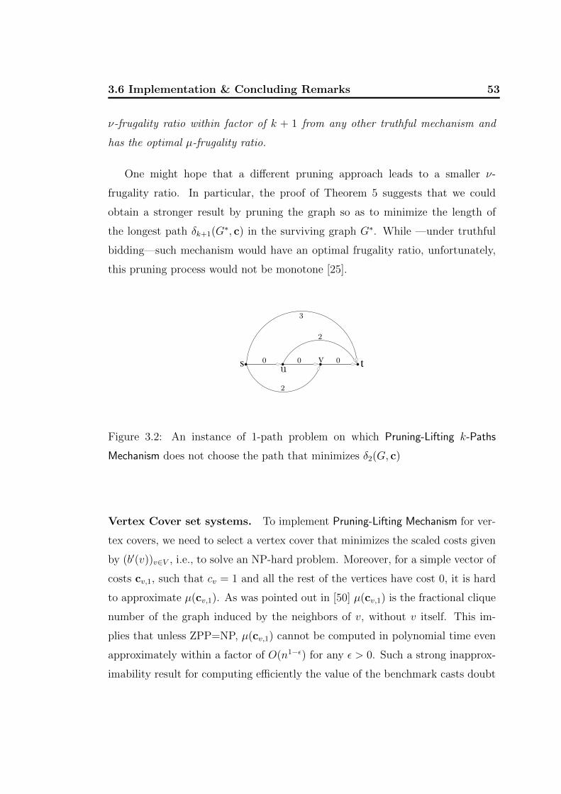
3.6 Implementation & Concluding Remarks 53
ν-frugality ratio within factor of k + 1 from any other truthful mechanism and
has the optimal µ-frugality ratio.
One might hope that a different pruning approach leads to a smaller ν-
frugality ratio. In particular, the proof of Theorem 5 suggests that we could
obtain a stronger result by pruning the graph so as to minimize the length of
the longest path δk+1(G∗, c) in the surviving graph G∗. While —under truthful
bidding—such mechanism would have an optimal frugality ratio, unfortunately,
this pruning process would not be monotone [25].
s t0
3
2
2
0 0vu
Figure 3.2: An instance of 1-path problem on which Pruning-Lifting k-Paths
Mechanism does not choose the path that minimizes δ2(G, c)
Vertex Cover set systems. To implement Pruning-Lifting Mechanism for ver-
tex covers, we need to select a vertex cover that minimizes the scaled costs given
by (b′(v))v∈V , i.e., to solve an NP-hard problem. Moreover, for a simple vector of
costs cv,1, such that cv = 1 and all the rest of the vertices have cost 0, it is hard
to approximate µ(cv,1). As was pointed out in [50] µ(cv,1) is the fractional clique
number of the graph induced by the neighbors of v, without v itself. This im-
plies that unless ZPP=NP, µ(cv,1) cannot be computed in polynomial time even
approximately within a factor of O(n1−ε) for any ε > 0. Such a strong inapprox-
imability result for computing efficiently the value of the benchmark casts doubt

54Chapter 3. Frugal Mechanism Design 2: Incentive Compatible
Mechanisms
on the existence of efficient truthful mechanism that performs almost as well as
the optimal mechanism and also casts doubt on the importance of an efficient
implementation in the frugality framework for vertex cover set systems.
On the positive side, the argument in Theorem 4 applies to any truthful
mechanism that selects a locally optimal solution, i.e., a vertex cover S that
satisfies b′(v) ≤∑
uv∈E,u 6∈S b′(u) for all v ∈ S. Paper [32] argues that any
monotone winner selection algorithm for vertex cover can be transformed into
a locally optimal one, and shows that a variant of the classic 2-approximation
algorithm for this problem [8] is monotone. This leads to a truthful polynomial
time mechanism, although with a hard-to-estimate ratio between its payment and
each of µ- or ν- benchmark.

Part II
Budget Feasible Mechanism
Design
55

Chapter 4Budget Feasible Mechanism Design 1:
Basic Model
4.1 The model
It is well-known that a mechanism may have to pay a large amount to enforce in-
centive compatibility (i.e., truthfulness). For example, as was discussed in Chap-
ter 2, the seminal VCG mechanism may have unbounded payment (compared to
the shortest path) in path auctions. The negative effect of truthfulness on pay-
ments leads to a study of frugal mechanism design, i.e., how should one minimize
his payment to get a feasible output with selfish agents? While we discussed a
few interesting instances of frugal mechanism design in the previous chapters, in
practice, one cannot expect to have big over payments for a few perspectives,
e.g., budget or resource limit.
Recently, Singer [63] initiated a study of mechanism design of reverse auctions
from a different prospective. Let us consider a procurement combinatorial auction
problem, where a buyer wishes to purchase some resources from a set of agents
A. Each agent i ∈ A is able to supply a resource at an incurred cost ci. The
buyer has a budget B that gives an upper bound on the compensation which
is distributed among agents, and a function v(·) describing the valuation that
57
58 Chapter 4. Budget Feasible Mechanism Design 1: Basic Model
the buyer obtains for every subset of A. This defines a natural optimization
problem: find a subset S ⊆ A that maximizes v(S) subject to∑
i∈S ci ≤ B.
Such combinatorial optimization problems have been considered in a variety
of domains. In particular, one may recall the following familiar optimization
problems:
Knapsack: Given a budget B and a set of items N = 1, . . . , n where each
item has a cost ci and a value vi, find a S ⊂ N , which maximizes∑
i∈S vi
and satisfies budget constraint∑
i∈S ci ≤ B.
Coverage: Given a budget B and subsets N = T1, . . . , Tn of a ground set,
each Ti with a cost ci, find a subset S ⊂ N that maximizes⋃i∈S Ti under
the budget constraint∑
i∈S ci ≤ B.
Matching: Given a budget B and graph G, where E(G) = e1, . . . , en and each
edge e has a cost ce and a value ve, find a matching S ⊂ E that maximizes∑e∈S ve under the budget constraint.
Knapsack and coverage problems fall in a more general framework of submod-
ular maximization, which received significant attention in the past few decades
(e.g. [58, 66, 51, 35, 53] consider submodular optimization with various condi-
tions).
Singer proposed studying these problems in a game theoretic scenario, where
one assumes agents to be self-interested entities so that each agent would want
to get as much subsidy as possible. In particular, an agent can conceal his true
incurred cost ci (which is known only to himself) and claim ‘any’ amount bi
instead. Thus, given submitted bids bi from all agents, a mechanism decides on
a winning set S ⊆ A and a payment pi to each winner i ∈ S. A mechanism is
called truthful (a.k.a. incentive compatible) if for every agent it is a dominant
strategy to bid his true cost, i.e., bi = ci. In this model we assume that agents
may behave strategically, whereas the buyer may not. We thus assume that the

4.1 The model 59
information related to the buyer, i.e., budget B and valuation function v(·), is a
public knowledge to everyone.
Our mechanism design problem has an important and practical ingredient: the
budget, i.e., the total payment of a mechanism should be upper bounded by B.
Although budget is a realistic condition that appears almost everywhere in daily
life, it has not received much attention until recently [29, 11, 15, 63, 21, 9, 7]. In
the framework of worst case analysis, most results are negative [29]. A possible
explanation for this could be that budget constraint introduces a new dimen-
sion to mechanism design and restricts the space of truthful mechanisms. For
example, in single-parameter domains where the private information of every in-
dividual is a single value (which is the case in our model), a monotone allocation
rule with associated threshold payments provides a sufficient and necessary con-
dition for truthfulness [57]. However, it may not necessarily generate a budget
feasible solution. Thus, a number of classic truthful designs as the seminal VCG
mechanism [68, 23, 42] do not apply, and new ideas have to be developed.
Another significant challenge due to the budget constraint is that, unlike the
VCG mechanism which always generates a socially optimal solution, we cannot
hope to have a solution that is both socially optimal and budget feasible even if
we are given unlimited computational power. Indeed, in a simple setting like path
procurement with 0 or 1 valuations [63], any budget feasible mechanism may have
an arbitrarily bad solution. Therefore, the question that one may ask is “under
which valuation domains do there exist truthful budget feasible mechanisms that
admit ‘small’ approximations (compared to the socially optimal solution)?”
The answer to this question depends on the properties of the valuation func-
tion under consideration. As the example of path procurement shows, a valuation
with complements does not work well in our framework. Therefore, it seems nat-
ural to focus on complement-free valuations. There is a broad classification of
various definitions of complement-free valuations briefly summarized in following

60 Chapter 4. Budget Feasible Mechanism Design 1: Basic Model
hierarchy [54]:
additive ⊂ gross substitutes ⊂ submodular
⊂ XOS ⊂ subadditive,
In this chapter we provide several constant approximations for the Addi-
tive(knapsack), Submodular (includes coverage problem), XOS (includes match-
ing) classes of valuations and give O(log n)-approximation for subbaditive v(·).The case of general subadditive valuations seems to be the most challenging and
interesting, as it was remarked in [30]:
“A fundamental question is whether, regardless of computational con-
straints, a constant-factor budget feasible mechanism exists for subad-
ditive functions.”
— Dobzinski, Papadimitriou, Singer
For the reader’s convenience we summarize the currently best known results
in the Table 4.1 below. We note that all randomized mechanism below are
universally truthful mechanisms, i.e., randomization is taken over deterministic
truthful mechanisms.
4.2 Preliminaries
In a marketplace there are n agents denoted by A = 1, . . . , n, each offering
a single item for sale. Each agent i has a privately known incurred cost ci (or
denoted by c(i)). We denote by c = (c(i))i∈A the cost vector of the agents. For any
given subset S ⊆ A of agents, there is a publicly known valuation v(S), meaning
the buyer’s welfare derived from S. We assume v(∅) = 0 and v(S) ≤ v(T ) for
any S ⊂ T ⊆ A.
We list below the definitions of various subclasses of complement-free valua-
tions moving from more basic classes to the most general one.

4.2 Preliminaries 61
Additive valuation Submodular valuation
deterministic randomized deterministic randomized
upper lower upper lower upper lower upper lower
Singer [63] 5 2 − − − 2 117.7 −
Chapter 4 2 +√
2 1 +√
2 3 2 8.34∗ 1 +√
2 7.91 2
*It may require exponential running time for general monotone submodular
functions.
XOS valuation Subadditive valuation
deterministic randomized deterministic randomized
Dobzinski et al. [30] − − O(log3 n) O(log2 n)
Chapter 4 − O(1) − O( lognlog logn
)
Table 4.1: Columns “Randomized” and “Deterministic” indicate whether a truth-
ful mechanism is allowed to use random coin flips. The columns “lower” and
“upper” denote the upper and lower bounds on approximation ratio obtained for
corresponding randomized or deterministic truthful mechanisms.
Additive: v(S) =∑
i∈S v(i) =∑
i∈S vi for any S ⊆ A.
Submodular: v(S) + v(T ) ≥ v(S ∩ T ) + v(S ∪ T ) for any S, T ⊆ A.
XOS: there is a set of additive functions f1, . . . , fm such that for any S ⊆ A
v(S) = maxf1(S), f2(S), . . . , fm(S)
.
Note that the number of functions m can be exponential in n = |A|.
Subadditive : v(S) + v(T ) ≥ v(S ∪ T ) for any S, T ⊆ A.
All three examples of the problems mentioned in Section 4.1 nicely fit into
these hierarchy of classes. In particular, the knapsack problem corresponds
exactly to the case of additive valuations, coverage is a special class of submodular

62 Chapter 4. Budget Feasible Mechanism Design 1: Basic Model
functions, and matching is an example of XOS valuation (for every legal matching
Mi of G let fi(S) =∑
e∈S∩Mivi).
An equivalent definition of submodular valuation can be formulated in terms
of the property of decreasing marginal returns, i.e., v(S ∪ i) − v(S) ≥ v(T ∪i)− v(T ) for any S ⊆ T ⊆ A and i ∈ A.
For XOS (a.k.a. fractionally subadditive) valuation there is also an equivalent
definition [34] ∀S ⊂ A:
v(S) ≤∑T⊆A
x(T ) · v(T )
s.t.∑
T⊆A: i∈Tx(T ) ≥ 1 ∀i ∈ S
0 ≤ x(T ) ≤ 1 ∀T ⊂ A
That is, if every element in S is fractionally covered, then the sum of the values
of all subsets weighted by the corresponding fractions is at least as large as v(S).
We note that the representation of a submodular/XOS/subadditive valuation
function usually requires exponential size in n. Thus, we assume that we are given
access to a demand oracle, which, for any given price vector p = (p1, . . . , pn),
returns us a subset
T ∈ argmaxS⊆A
(v(S)−
∑i∈S
p(i)
).
Every such a query is assumed to take unit time. The demand oracle is used in [30]
as well, and it was shown that a weaker value query oracle is not sufficient [63].
Upon receiving a bid cost bi from each agent, a mechanism decides upon an
allocation S ⊆ A as winners and a payment pi to each i ∈ A. We assume that
a mechanism may not make positive transfers (i.e., pi = 0 if i /∈ S) and is
individually rational (i.e., pi ≥ bi if i ∈ S). Agents bid strategically on their
costs and would like to maximize their quasi-linear utilities, which are given for
every agent i as pi − ci, if i is a winner, and 0 otherwise. We say a mechanism is
incentive compatible or truthful if it is in the best interest for each agent to report
his true cost. For randomized mechanisms, we consider universal truthfulness in

4.3 Additive Valuation. 63
this paper (i.e., a randomized mechanism takes a distribution over deterministic
truthful mechanisms).
Our setting is in single parameter domain, as each agent has only one cost to
report on. For single parameter domains it is well-known [57] that a mechanism
is truthful if and only if its allocation rule is monotone (i.e., a winner keeps
winning if he unilaterally decreases his bid) and the payment to each winner is
his threshold bid (i.e., the maximal bid for which the agent still wins). Therefore,
we will only focus on designing monotone allocations and do not specify the
payment to each winner explicitly. Although we will always implicitly verify that
the total payment is below the budget B.
A mechanism is said to be budget feasible if∑
i pi ≤ B on every instance of
bids and randomness in the mechanism, where B is a given budget constraint.
Assume without loss of generality that ci ≤ B for any agent i ∈ A, since otherwise
he would never win in any (randomized) budget feasible truthful mechanism.
Our objective is to design truthful budget feasible mechanisms with every output
being approximately close to the social optimum. That is, we want to minimize
the approximation ratio of a mechanism, which is defined as maxI
opt(I)M(I)
, where
M(I) is the (expected) value of mechanism M on instance I and opt(I) is the
optimal value of the integer program: maxS⊆A v(S) subject to c(S) ≤ B, where
c(S) =∑
i∈S ci.
4.3 Additive Valuation.
We consider here the most basic case where the valuation of the buyer is additive,
i.e., v(S) =∑
i∈S vi for any S ⊆ A. This leads to an instance of Knapsack prob-
lem, where items correspond to agents and the size of the knapsack corresponds
to budget B.
We present below two truthful mechanism, one with randomized and another

64 Chapter 4. Budget Feasible Mechanism Design 1: Basic Model
one with deterministic implementations. Our randomized mechanism is univer-
sally truthful, meaning that for any fixed realization of the random coin flips the
mechanism is truthful as a deterministic mechanism.
4.3.1 Deterministic Mechanism.
We consider the following greedy strategy studied by Singer [63].
Greedy-KS(A)
1. Order all items in A s.t. v1c1≥ v2
c2≥ · · · ≥ v|A|
c|A|
2. Let k = 1 and S = ∅
3. While k ≤ |A| and ck ≤ B · vk∑i∈S∪k vi
S ← S ∪ k
k ← k + 1
4. Return winning set S
It is shown that the above greedy strategy is monotone (and therefore truthful).
Actually, it has the following remarkable property: any i ∈ S cannot control the
output set, given that i is guaranteed to be a winner. That is, if the winning sets
are S and S ′, provided that i bids ci and c′i, respectively, where i ∈ S ∩ S ′, then
S = S ′.
Otherwise, let i0 be the item with the smallest index in (S \ S ′) ∪ (S ′ \ S).
Without loss of generality let us assume i0 ∈ S \ S ′. That only could happen, if
i0 appeared earlier in S than i and i0 was rejected from S ′ after i has been taken
into S ′. Let T = j ∈ S ∩ S ′ | j < i0, j 6= i be the winning items in S ∩ S ′ \ ibefore i0. Since i got accepted in S claiming the cost ci after i0, we have
vi0ci0≥ vici≥
∑j∈S,j≤i)
vj
B≥∑
j∈T vj + vi + vi0
B.

4.3 Additive Valuation. 65
Rewriting the above inequality, we get
ci0 ≤ B · vi0∑j∈T vj + vi + vi0
,
which implies that i0 should be a winner in S ′ as well, a contradiction.
Given the greedy strategy described above, our mechanism for knapsack is
as follows (where fopt(A) denotes the value of the optimal fractional solution to
knapsack, which can be computed in polynomial time).
Deterministic-KS
1. Let A = i | ci ≤ B and i∗ ∈ argmaxi∈A vi
2. If (1 +√
2) · vi∗ ≥ fopt(A \ i∗), return i∗
3. Otherwise, return S = Greedy-KS(A)
Theorem 11. Deterministic-KS is a deterministic budget feasible truthful mecha-
nism that is a 2 +√
2 approximation for any additive valuations.
Proof. The proof proceeds by verifying each property stated in the claim.
Truthfulness. We analyze monotonicity of the mechanism according to the
condition of Steps 2 and 3, respectively. If i∗ wins in Step 2 (note that the
fractional optimal value computed in Step 2 is independent of the bid of
i∗), then i∗ still wins if he decreases his bid.
If the condition in Step 2 fails and the mechanism continues to Step 3,
for any i ∈ S, the subset S remains the same if i decreases his bid. Note
that if i 6= i∗, when i decreases his bid, the value of the fractional optimal
solution computed in Step 2 will not decrease. Hence i is still a winner,
which implies that the mechanism is monotone and, therefore, combined
with the threshold payments is incentive compatible.

66 Chapter 4. Budget Feasible Mechanism Design 1: Basic Model
Individual rationality and budget feasibility. If i∗ wins in Step 2, his payment
is the threshold bid B. Otherwise, assume that all sellers in A are ordered
by 1, 2, . . . , n; let S = 1, . . . , k. Note that it is possible that i∗ ∈ S. For
any i ∈ S, let qi be the maximum cost that i can bid such that the fractional
optimal value on instance A\i∗ is still larger than (1+√
2)vi∗ . Note that
ci ≤ qi.
Thus, the payment to any winner is
pi = min
vi ·
ck+1
vk+1
, B · vi∑j∈S vj
, qi
, i ∈ S \ i∗
and
pi∗ = min
vi∗ ·
ck+1
vk+1
, B · vi∗∑j∈S vj
, if i∗ ∈ S.
Further,∑
i∈S pi ≤∑
i∈S B ·vi∑j∈S vj
= B, which implies that the mechanism
is budget feasible. The mechanism is individually rational, since we use a
threshold payment rule.
Approximation. Assume that all sellers in A are ordered by 1, 2, . . . , n,
and T = 1, . . . , k is the subset returned by Greedy-KS(A). Let ` be the
maximal item for which∑
i=1,...,` ci ≤ B. Let c′`+1 = B −∑
i=1,...,` ci and
v′`+1 = v`+1 ·c′`+1
c`+1. Hence, the optimal fractional solution is
fopt(A) =∑i=1
vi + v′`+1.
For any j = k + 1, . . . , `, we have
cjvj≥ ck+1
vk+1
>1
vk+1
·B · vk+1∑k+1i=1 vi
,
where the last inequality follows from the fact that the greedy strategy
stops at item k + 1. Hence, cj > B · vj∑k+1i=1 vi
. Asc′`+1
v′`+1= c`+1
v`+1, we have
c′`+1 > B · v′`+1∑k+1i=1 vi
. Therefore,

4.3 Additive Valuation. 67
B ·∑`
j=k+1 vj + v′`+1∑k+1i=1 vi
<∑j=k+1
cj + c′`+1 < B,
which implies that∑k
i=1 vi >∑`
j=k+2 vj + v′`+1. Hence
fopt(A) =∑i=1
vi + v′`+1 < 2∑i∈S
vi + vi∗ .
The following are some basic properties of the optimal fractional solution
fopt(A)− vi∗ ≤ fopt(A \ i∗) ≤ fopt(A)
Hence, if the condition in Step 2 holds and the mechanism outputs i∗, we
have
fopt(A) ≤ fopt(A \ i∗) + vi∗ ≤ (2 +√
2) · vi∗
On the other hand, if the mechanism outputs S in Step 3, we have
(1 +√
2) · vi∗ < fopt(A \ i∗)
≤ fopt(A)
< 2∑i∈S
vi + vi∗
which implies that vi∗ <√
2 ·∑
i∈S vi. Hence,
opt(A) ≤ fopt(A) =∑
i=1,...,`
vi + v′`+1
< 2∑i∈S
vi + vi∗
≤ (2 +√
2) ·∑i∈S
vi.
Therefore, Deterministic-KS has approximation ratio of at most (2 +√
2) .
68 Chapter 4. Budget Feasible Mechanism Design 1: Basic Model
4.3.2 Randomized Mechanism.
Our randomized mechanism for knapsack is as follows.
Random-KS
1. Let A = i | ci ≤ B and i∗ ∈ argmaxi∈A vi
2. With probability 13, return i∗
3. With probability 23, return Greedy-KS(A)
Theorem 12. Random-KS is a universal truthful budget feasible mechanism that
is a 3 approximation for any additive valuation.
Proof. Since both mechanisms in Steps 2 and 3 are budget feasible and truthful,
it remains to establish the approximation ratio.
Using the same notation and argument as in the proof of Theorem 11,
assume that all sellers in A are ordered from 1 to n, and T = 1, . . . , k is
the subset returned by Greedy-KS(A). Let ` be the maximal-value item for which∑i=1,...,` ci ≤ B. Let c′`+1 = B −
∑i=1,...,` ci and v′`+1 = c′`+1 ·
v`+1
c`+1. Hence, the
optimal fractional solution is
fopt(A) =∑i=1
vi + v′`+1
and
fopt(A) =∑i=1
vi + v′`+1 < vi∗ + 2∑i∈S
vi.
The expected value of Random-KS is therefore
1
3vi∗ +
2
3
∑i∈S
vi =1
3
(vi∗ + 2
∑i∈S
vi
)>
1
3opt.

4.4 Lower Bounds 69
4.4 Lower Bounds
In this section we discuss the lower bounds on the approximation ratio of truthful
budget feasible mechanisms for additive valuations. In [63], a lower bound of 2 is
obtained by the following argument. Consider the case with two items, each of
value 1. If their costs are (B − ε, B − ε), at least one item should win, otherwise
the approximation ratio is infinite. Without loss of generality, one can assume
that the first item wins, and as a result its payment is at least B−ε. Now consider
another profile (ε, B − ε), the first item must win (due to monotonicity) and get
a payment of at least B − ε due to truthfulness. The second item then does not
win because of the budget constraint and individual rationality. Therefore, the
mechanism may only achieve a value of 1 for such instance while the optimal
solution is 2. This gives us the lower bound of 2.
We improve the deterministic lower bound to 1 +√
2 by a more involved
argument. We also provide a lower bound of 2 for any randomized universally
truthful mechanism. All these lower bounds are unconditional, i.e., one does not
impose any complexity assumptions and constraints on the running time of the
mechanism.
4.4.1 Lower Bound for Deterministic Mechanisms
Theorem 13. No deterministic truthful budget feasible mechanism can achieve
an approximation ratio better than 1 +√
2, even if there are only three items.
Assume otherwise that there is a budget feasible truthful mechanism that can
achieve a ratio better than 1 +√
2. We consider the following scenario: budget
B = 1, and values v1 =√
2, v2 = v3 = 1. Then the mechanism for any bidding
scenario satisfies the following two properties:
if all items are winners in the optimal solution, the mechanism must output
at least two items;

70 Chapter 4. Budget Feasible Mechanism Design 1: Basic Model
if 1, 2 or 1, 3 is the optimal solution, the mechanism cannot output
either 2 or 3 (i.e., a single item with unit value).
For any item i, let function pi(cj, ck) be the payment offered to item i given that
the bids of the other two items are cj and ck. That is, pi(cj, ck) is the threshold
bid of i to be a winner.
Lemma 7. For any c3 > 0.5 and any domain (a, b) ⊂ (0, 1 − c3), there is
c2 ∈ (a, b) such that p1(c2, c3) < 1− c2.
Proof. Assume otherwise that there are c3 > 0.5 and (a, b) ⊂ (0, 1 − c3) such
that for any c2 ∈ (a, b), p1(c2, c3) ≥ 1 − c2. Let c1 = 1 − c3 − b. Then
c1 + c2 + c3 < 1 = B, which implies that the mechanism has to output at
least two items. Since 0 < c1 = 1 − c3 − b < 1 − c2 ≤ p1(c2, c3), item 1 is a
winner. Further, p1(c2, c3) ≥ 1− c2 > 0.5, which together with budget feasibility
implies that item 3 cannot be a winner. Therefore, item 2 must be a winner with
payment p2(c1, c3) = c2 due to individual rationality and budget feasibility. The
same analysis still holds if the true cost of item 2 becomes c′2 = c2+b2
, i.e., item
2 is still a winner with payment c′2. Thus for the sample (c1, c2, c3) the payment
satisfies p2(c1, c3) ≥ c′2 > c2, a contradiction.
Since items 2 and 3 are identical, the above lemma still holds if we switch
items 2 and 3 in the claim. We are now ready to prove Theorem 13.
Proof of Theorem 13. Define c3 = 0.7 and (a, b) = (0.2, 0.3). Note that c3
and (a, b) satisfy the condition of Lemma 7. Hence, there is c ∈ (0.2, 0.3)
such that p1(c, 0.7) < 1 − c. Define p1(c, 0.7) = 1 − c − x, where x > 0.
Symmetrically, define c2 = 0.7 and (a′, b′) = (c,min0.3, c + x). Again by
Lemma 7, there is d ∈ (a′, b′) such that p1(0.7, d) < 1 − d. Define p1(0.7, d) =
1 − d − y, where y > 0. Pick c1 = 1 − d − ε, where ε > 0 is sufficiently small so
that c1 ∈ (1− c− x, 1− c) ∩ (1− d− y, 1− d). Note that since d ∈ (c, c+ x), c1
is well-defined.

4.4 Lower Bounds 71
Consider a true cost vector (c1, c, 0.7). Since p1(c, 0.7) = 1− c− x < c1, item
1 cannot be a winner. Since c1 + c = 1− d− ε+ c < 1, the optimal solution has
a value of at least v1 + v2 = 1 +√
2; therefore the mechanism has to output both
items 2 and 3. Hence, p3(c1, c) ≥ c3 = 0.7.
Similarly, consider true cost vector (c1, 0.7, d); we have p2(c1, d) ≥ c2 = 0.7.
Finally, consider cost vector (c1, c, d). By the above two inequalities, both items
2 and 3 are the winners; this contradicts the budget feasibility.
4.4.2 Lower Bound for Randomized Mechanisms
Theorem 14. No randomized (universally) truthful budget feasible mechanism
can achieve an approximation ratio better than 2, even in the case of two items.
Proof. We use Yao’s min-max principle, which is a typical tool used to prove lower
bounds, where we need to design a distribution of instances and argue that any
deterministic budget feasible mechanism cannot get an expected approximation
ratio better than 2.
All the instances contain two items of value 1. Their costs (c1, c2) are drawn
from the following distribution (see Fig. 4.1 for an example):
1. (kBn, (n−k)B
n) with probability 1−ε
n−1, where k = 1, 2, . . . , n− 1,
2. ( iBn, jBn
) with probability 2ε(n−1)(n−2)
, where i, j ∈ 1, . . . , n−1 and i+j > n,
where 1 > ε > 0 and n is a large integer.
We first claim that for any deterministic truthful budget feasible mechanism
with finite expected approximation ratio, there is at most one instance, for which
both items win in the mechanism. Assume by contradiction that there are at
least two such instances. Note that for the second distribution ( iBn, jBn
), where
i+ j > n, it cannot be the case that both items win due to the budget constraint.
Hence, the two instances must be of the first type; denote them by (k1Bn, (n−k1)B
n)
and (k2Bn, (n−k2)B
n), where k1 > k2. Consider the instance (k1B
n, (n−k2)B
n) . Since

72 Chapter 4. Budget Feasible Mechanism Design 1: Basic Model
c2
c11
1
k2
nk1
n
Figure 4.1: Distribution for n = 6. Diameter of a point emphasizes its probability.
k1 + n − k2 > n, this is the instance of the second type in our distribution.
Therefore it has nonzero probability (see Fig. 4.1). The mechanism has a finite
approximation ratio, thus it should have a finite approximation ratio on the
instance (k1Bn, (n−k2)B
n) as well. As a result, it cannot be the case that both
items lose. We assume that item 1 wins (the proof for the other case is similar);
the payment to him is at least k1Bn
due to individual rationality. Then consider
the original instance (k2Bn, (n−k2)B
n); item 1 should also win and get a threshold
payment, which is equal to or greater than k1Bn
. Therefore the payment to the
second item is at most B− k1Bn
= (n−k1)Bn
because of the budget constraint. Since(n−k1)B
n< (n−k2)B
n, we arrive at a contradiction with either individual rationality
or with the assumption that both items won in the instance (k2Bn, (n−k2)B
n).
On the other hand, for all instances (kBn, (n−k)B
n), both items win in the
optimal solution with value 2. Hence, the expected approximation ratio of any
deterministic truthful budget feasible mechanism is at least 1−εn−1·1+(n−2) · 1−ε
n−1·
2 + ε · 1 = 2− ε− 1−εn−1
. The ratio approaches 2 as ε→ 0 and n→∞.

4.5 Submodular Valuations 73
4.5 Submodular Valuations
For any given monotone submodular function, we denote the marginal contribu-
tion of an item i with respect to set S by mS(i) = v(S ∪ i)− v(S). We assume
that agents are sorted according to their non-increasing marginal contributions
relative to their costs, recursively defined by: i+ 1 = argmaxj∈A\SimSi (j)
cj, where
Si = 1, . . . , i and S0 = ∅. To simplify notations we will denote this order by [n]
and write mi instead of mSi−1(i). This sorting, in the presence of submodularity,
implies thatm1
c1
≥ m2
c2
≥ · · · ≥ mn
cn.
Notice that v(Sk) =∑
i≤kmi for all k ∈ [n].
The following greedy scheme is the core of our mechanism (where the param-
eters denote the set of agents A and available budget B/2).
Greedy-SM(A,B/2)
1. Let k = 1 and S = ∅
2. While k ≤ |A| and ck ≤ B2 ·
mk∑i∈S∪kmi
S ← S ∪ k
k ← k + 1
3. Return winning set S
4.5.1 Randomized Mechanism
Our mechanism for general monotone submodular functions is as follows.1
1Our mechanism has a similar flavor to Singer’s mechanism [63] for the greedy scheme and
randomness between the greedy and the item with the largest value. Indeed, both arise from
the algorithm that maximizes monotone submodular functions with weighted items [51]. Our
mechanism, however, treats the greedy scheme and random selection in a slightly different way,
which yields a much better approximation ratio.

74 Chapter 4. Budget Feasible Mechanism Design 1: Basic Model
Random-SM
1. Let A = i | ci ≤ B and i∗ ∈ argmaxi∈A v(i)
2. with probability 0.4, return i∗
3. with probability 0.6, return Greedy-SM(A,B/2)
In the above mechanism, if it returns i∗, the payment to i∗ is B; if the
mechanism returns Greedy-SM(A,B/2), the payments are the threshold bids and
are explicitly derived in [63]. Actually, in our analysis we do not need this explicit
payment formula.
Theorem 15. Random-SM is a budget feasible universally truthful mechanism
for a submodular valuation function with an approximation ratio of 5ee−1
(≈ 7.91).
Proof. The proof proceeds by verifying each property of the mechanism.
Universal Truthfulness. Our mechanism is a simple random combination of
two mechanisms. To prove that the Random-SM is universally truthful, it suffices
to prove that these two mechanisms are truthful respectively, i.e., the allocation
rule is monotone.
The scheme where we simply return i∗ is obviously truthful. Also it is easy
to see that throwing away agents with a cost greater than B in the prior step
does not affect truthfulness. The greedy scheme Greedy-SM(A,B/2) is monotone
as well, since any item out of a winning set cannot increase its bid to become a
winner.
Budget Feasibility. While truthfulness is quite straightforward, the budget
feasibility analysis turns out to be quite tricky. The difficulties arise while we
compute the payment to each item. Indeed, it may happen that an agent changes
his bid (while remaining in the winning set) and make the mechanism to change
its output. In other words, computing the threshold bid of an item, we need to
4.5 Submodular Valuations 75
look at quite different outputs of the mechanism. Fortunately, in such a case no
item can reduce the valuation of the output too much. That enables us to write
down an upper bound on the bid of each item in the case of submodular valuation
and obtain budget feasibility by summing up these bounds.
If the mechanism returns i∗, the agent’s payment is B, which is clearly budget
feasible. We are left to prove budget feasibility for Greedy-SM(A,B/2). A similar
but a weaker result has been proven in [63], using the characterization of payments
and arguing that the total payment is not larger than B. Here we directly show
that the payment to any item i in the winning set S is bounded above by miv(S)·B;
then the total payment will be bounded by B since∑i∈Smiv(S)
·B = B. Before doing
that, we first prove a useful lemma.
Lemma 8. Let S ⊂ T ⊆ [n] and t0 = argmaxt∈T\SmS(t)c(t)
. Then
v(T )− v(S)
c(T )− c(S)≤ mS(t0)
c(t0).
Proof. Assume by contradiction that the lemma does not hold. Then
v(T )− v(S)
c(T )− c(S)>mS(t)
c(t), for all t ∈ T \ S.
Summing up all the inequalities, each multiplied by c(t)∑t∈T\S c(t)
, we have
v(T )− v(S)
c(T )− c(S)>
∑t∈T\SmS(t)∑t∈T\S c(t)
=
∑t∈T\SmS(t)
c(T )− c(S).
This implies that v(T )− v(S) >∑
t∈T\SmS(t), which contradicts the submodu-
larity.
Let 1, . . . , k be the order of items in which we add them to the winning set.
Let ∅ = S0 ⊂ S1 ⊂ . . . ⊂ Sk ⊆ [n] be the sequence of winning sets that we pick at
each step by applying our mechanism. Thus we have Sj = 1, . . . , j = [j]. Now,
since v(·) is sumbodular, we can write the following chain of inequalities (note
that marginal contribution is smaller for larger sets).
mS0(1)
c1
≥ mS1(2)
c2
≥ . . . ≥mSk−1
(k)
ck≥ 2v(Sk)
B,
76 Chapter 4. Budget Feasible Mechanism Design 1: Basic Model
where the last inequality holds true due to Lemma 8 and the fact that c(Sk) ≤ B2
.
The following lemma concludes the proof of budget feasibility, since it shows
that payment to each winning agent j does not exceed mSj−1(j) B
v(S).
Lemma 9. No agent j ∈ S = Greedy-SM(A,B/2) could bid more than mSj−1(j) B
v(S)
and be in the winning set.
Proof. Assume that S = Sk is the winning set and there is j ∈ Sk such that it can
bid bj > mSj−1(j) B
v(Sk)and still win (given fixed bids of others). In the following
we will use b instead of c to denote that we are considering a new scenario where
an agent j has increased his bid to bj and bids of other agents remain the same
(bi = ci for i 6= j).
Note that
mS0(1)
c1
≥ mS1(2)
c2
≥ . . . ≥mSj−1
(j)
cj≥mSj−1
(j)
bj.
For a bid vector b, we denote by T ⊇ Sj−1 the set of agents chosen earlier
than j in the winning set. Thus, by the rule of the greedy mechanism, we have
j = argmaxi∈[n]\T
mT (i)
bi, (4.1)
mT (j)
bj≥ 2v(T ∪ j)
B. (4.2)
We may assume Sk ∪ T ) T ∪ j. Indeed, otherwise T ∪ j = Sk ∪ T and
mSj−1(j)
bj≥ mT (j)
bj≥ 2v(T ∪ j)
B≥ 2v(Sk)
B≥ v(Sk)
B.
Thus bj ≤ mSj−1
Bv(Sk)
and we get a contradiction.
Let R = Sk \T . Applying equation (4.1) and Lemma 8 to Sk∪T and T ∪j,we know that for some r0 ∈ R \ j,
v(Sk ∪ T )− v(T ∪ j)b(Sk ∪ T )− b(T ∪ j)
≤mT∪j(r0)
b(r0)≤ mT (r0)
b(r0)≤ mT (j)
bj.
On the other hand, since bj > mSj−1(j) B
v(Sk), we have
mT (j)
bj<
mT (j)
mSj−1(j)
v(Sk)
B<v(Sk)
B.

4.5 Submodular Valuations 77
Combining these inequalities, we get
v(Sk ∪ T )− v(T ∪ j)b(Sk ∪ T )− b(T ∪ j)
<v(Sk)
B.
We have
b(Sk ∪ T )− b(T ∪ j) = b(R \ j) = c(R \ j) ≤ c(Sk).
Recall thatmSi−1
(i)
ci≥ 2v(Sk)
Bfor i ∈ [k]. Thus ci ≤ mSi−1
(i) B2v(Sk)
and
c(Sk) =∑k
i=1 c(i) ≤B2. We get
v(Sk)− v(T ∪ j)B/2
≤ v(Sk)− v(T ∪ j)c(Sk)
≤ v(Sk ∪ T )− v(T ∪ j)b(Sk ∪ T )− b(T ∪ j)
<v(Sk)
B.
Thus, v(Sk) < 2v(T ∪ j). Finally, we derive
mSj−1(j)
bj≥ mT (j)
bj≥ 2v(T ∪ j)
B>v(Sk)
B,
which contradicts with bj > mSj−1(j) B
v(Sk).
Approximation Ratio. Throughout this part we need not bother with incen-
tives issues and focus only on the approximation guarantees.
Before analyzing the performance of our mechanism, we consider the following
simple greedy algorithm: order items according to their marginal contributions
divided by costs and add as many items as possible (i.e., it stops when we cannot
add the next item as the sum of ci will exceed B). Moreover, we may consider
the fractional variant of that scheme, i.e., on the all remaining budget we buy
an affordable fraction of the last item. Let ` be the maximal index for which∑i=1,...,` ci ≤ B. Let c′`+1 = B −
∑i=1,...,` ci and m′`+1 = m`+1 ·
c′`+1
c`+1. Hence, the
fractional greedy solution is defined as
fgre(A) ,∑i=1
mi +m′`+1.

78 Chapter 4. Budget Feasible Mechanism Design 1: Basic Model
It is well-known that the greedy algorithm is a 1−1/e approximation for max-
imization of a monotone submodular functions with a cardinality constraint [58].
Also it was shown that the simple greedy algorithm may have an unbounded
approximation ratio in case of weighted items with a capacity constraint. Nev-
ertheless, a variant of greedy algorithm was suggested in [51] which gives the
same 1 − 1/e approximation to the weighted case. The following lemma, which
is fundamental in our analysis, establishes the same approximation ratio for the
fractional greedy algorithm described above.
Lemma 10. The fractional greedy solution has an approximation ratio of 1−1/e
for the weighted submodular maximization problem. That is,
fgre(A) ≥ (1− 1/e) · opt(A),
where opt(A) is the value of the optimal integral solution for the given instance
A.
Proof. Recall that ci denotes the cost of each item i ∈ [n]. Our goal in the
weighted problem is to pick a set S with total cost∑
i∈S ci not exceeding
given budget B of maximal possible value v(S), where v is the given monotone
submodular function. As the value vf (Sf ) is for fractional problem we consider
the expectation of v(S), where each i ∈ [n] is selected at random independently
in S with probability equal to the fraction of item i in Sf .
Assume that all costs ci are integers. We reduce our weighted problem with
monotone submodular function v to the unweighted one as follows.
For each item i ∈ [n] we consider ci new items of unit cost. Denote them
as ij for j ∈ [ci] and call i the type of the unit ij.
The new valuation function µ only depends on the amounts of unit items
of each type.

4.5 Submodular Valuations 79
Let a set S contain ai units of each type i. Independently for each type,
pick at random in the set R with probability aici
weighted item i. Define
µ(S) = E(v(R)).
Therefore
µ(S) =1
c1 · . . . · cn
∑π
v (S · π) (4.3)
where π is a sampling of units, one for each type (there are c1 · . . . · cn variants
for π); S · π is a vector of types for which sample π is an element of S.
Using (4.3) it is not hard to verify monotonicity and submodularity of µ.
Indeed, e.g. to verify submodularity one only needs to check that the marginal
contribution of any unit is smaller for a large set, i.e., for S ⊂ T and ij /∈ T verify
inequality µ(S ∩ ij)− µ(S) ≥ µ(T ∩ ij)− µ(T ).
For any T ⊆ [n] if we consider the set of units S = ik|i ∈ T, 1 ≤ k ≤ ci.Then according to the definition µ(S) = v(T ). Hence, the optimal solution to the
unit costs problem is equal to or larger than the optimal solution to the original
problem.
It remains to show that our fractional greedy scheme for an integer weighted
instance gives us the same result as the greedy scheme for its unit weighted
version. Note that once we have taken a unit of type i we will proceed to take
units of type i until its supply gets exhausted completely (we break ties in favor
of the last type we have picked). Indeed, let ik, ik+1 /∈ S then
µ(S ∪ ik)− µ(S) = µ(S ∪ ik+1)− µ(S)
=1∏nj=1 cj
∑π|ik+1∈π
v (S ∪ ik+1 · π)− v (S · π)
=1∏nj=1 cj
∑π|ik+1∈π
v (S ∪ ik, ik+1 · π)− v (S ∪ ik · π)
= µ(S ∪ ik, ik+1)− µ(S ∪ ik)
Therefore, the marginal contribution of the type i does not decrease if we in-
clude units of type i in the solution. On the other hand, because µ is submodular,
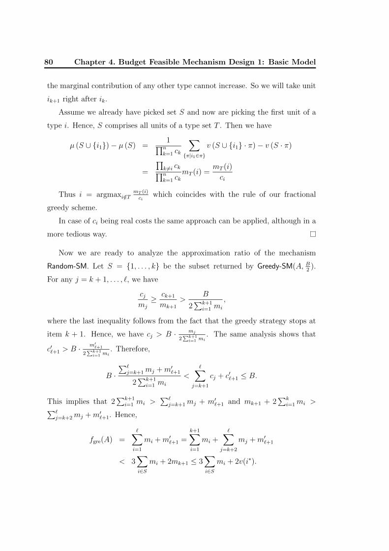
80 Chapter 4. Budget Feasible Mechanism Design 1: Basic Model
the marginal contribution of any other type cannot increase. So we will take unit
ik+1 right after ik.
Assume we already have picked set S and now are picking the first unit of a
type i. Hence, S comprises all units of a type set T . Then we have
µ (S ∪ i1)− µ (S) =1∏nk=1 ck
∑π|i1∈π
v (S ∪ i1 · π)− v (S · π)
=
∏k 6=i ck∏nk=1 ck
mT (i) =mT (i)
ci
Thus i = argmaxi/∈TmT (i)ci
which coincides with the rule of our fractional
greedy scheme.
In case of ci being real costs the same approach can be applied, although in a
more tedious way.
Now we are ready to analyze the approximation ratio of the mechanism
Random-SM. Let S = 1, . . . , k be the subset returned by Greedy-SM(A, B2
).
For any j = k + 1, . . . , `, we have
cjmj
≥ ck+1
mk+1
>B
2∑k+1
i=1 mi
,
where the last inequality follows from the fact that the greedy strategy stops at
item k + 1. Hence, we have cj > B · mj
2∑k+1i=1 mi
. The same analysis shows that
c′`+1 > B · m′`+1
2∑k+1i=1 mi
. Therefore,
B ·∑`
j=k+1mj +m′`+1
2∑k+1
i=1 mi
<∑j=k+1
cj + c′`+1 ≤ B.
This implies that 2∑k+1
i=1 mi >∑`
j=k+1mj + m′`+1 and mk+1 + 2∑k
i=1mi >∑`j=k+2mj +m′`+1. Hence,
fgre(A) =∑i=1
mi +m′`+1 =k+1∑i=1
mi +∑j=k+2
mj +m′`+1
< 3∑i∈S
mi + 2mk+1 ≤ 3∑i∈S
mi + 2v(i∗).

4.5 Submodular Valuations 81
Together with Lemma 10, it bounds the optimal solution as
opt(A) ≤ e
e− 1
(3Greedy-SM(A,B/2) + 2v(i∗)
). (4.4)
The expected value of our randomized mechanism is 35Greedy-SM(A,B/2) +
25v(i∗) ≥ e−1
5eopt.
4.5.2 Deterministic Mechanism.
Here we provide a deterministic truthful mechanism which is budget feasible
and has a constant approximation ratio. In the following description opt(A \i∗, B) denotes the value of the optimal solution of the weighted submodular
maximization problem for the set of agents A \ i∗ and budget B.
Deterministic-SM
1. Let A = i | ci ≤ B and i∗ ∈ argmaxi∈A v(i)
2. If 1+4e+√
1+24e2
2(e−1) · v(i∗) ≥ opt(A \ i∗, B), return i∗
3. Otherwise, return Greedy-SM(A,B/2)
This deterministic mechanism does not work in polynomial time because of the
computational hardness of submodular maximization problem. We note however
that one cannot replace optimal solution by a greedy solution in the above
mechanism as it may break monotonicity. Indeed, unlike the case of additive
valuations a seller may change his bid and influence the outcome of a greedy
algorithm, while remaining in the winning set. In contrast to frugality model
for vertex cover set systems, where we have an efficient greedy algorithm with
constant approximation ratio and monotone selection rule, we don’t know if such
a mechanism exists in the case of general submodular valuations.
Theorem 16. Deterministic-SM is a deterministic budget feasible truthful mecha-
nism for monotone submodular functions with an approximation ratio of (≈ 8.34)
6e−1+√
1+24e2
2(e−1).

82 Chapter 4. Budget Feasible Mechanism Design 1: Basic Model
Proof. We note that the bid of i∗ is independent of the value of opt(A \ i∗, B).
The similar argument as in the proof of Theorem 11 gives us truthfulness.
Budget feasibility follows from Lemma 9 and observation that Step 2 only sets
additional thresholds on the payments of Greedy-SM(A,B/2).
In what follows, we prove the approximate ratio. Let
x =1 + 4e+
√1 + 24e2
2(e− 1)(≈ 7.34).
We observe that
opt(A,B)− v(i∗) ≤ opt(A \ i∗, B) ≤ opt(A,B).
If the condition in Step 2 holds and the mechanism outputs i∗, then
opt(A,B) ≤ opt(A \ i∗, B) + v(i∗) ≤ (x+ 1) · v(i∗).
In the other case we run Greedy-SM(A,B/2). We apply (4.4) and get
x · v(i∗) < opt(A \ i∗, B) ≤ opt(A,B)
≤ e
e− 1
(3Greedy-SM(A,B/2) + 2v(i∗)
).
This implies that
v(i∗) ≤ 3e
x(e− 1)− 2eGreedy-SM(A,B/2).
Hence,
opt ≤ e
e− 1
(3Greedy-SM(A,B/2) + 2v(i∗)
)≤ e
e− 1
(3 +
6e
x(e− 1)− 2e
)· Greedy-SM(A,B/2).
Simple calculations show that
1 + x =6e− 1 +
√1 + 24e2
2(e− 1)
=e
e− 1
(3 +
6e
x(e− 1)− 2e
).
Therefore, we have opt ≤ (x + 1) · Greedy-SM(A,B/2) in the both cases, which
concludes the proof of the claimed approximation ratio.

4.6 XOS Valuations 83
4.6 XOS Valuations
We recall the definition of XOS valuation v(·): for any S ⊆ A
v(S) = max f1(S), f2(S), . . . , fm(S) ,
where each fj(·) is a nonnegative additive function, i.e., fj(S) =∑
i∈S fj(i).
We assume w.l.o.g. that ci ≤ B for any agent i ∈ A, since if ci > B, then
such an agent would never win in any budget feasible mechanism.
Below we establish the main component of our main XOS mechanism. We use
randomized Additive-mechanism for additive valuations as an auxiliary procedure,
where Additive-mechanism is an universally truthful mechanism Random-KS from
Section 4.3 with an approximation factor of at most 3.
XOS-random-sample
1. Sample items independently at random with probability 12
in group T.
2. Find optimal solution opt(T ) for item set T and budget B.
3. Set a threshold t = v(opt(T ))8B .
4. For items in A \ T find a set S∗ ∈ argmaxS⊆A\T
v(S)− t · c(S)
.
5. Find additive f ∈ f1, . . . , fm, s.t. f(S∗) = v(S∗).
6. Run Additive-mechanism for f(·), item set S∗, budget B.
7. Output the result of Additive-mechanism.
In the above mechanism, we first sample half in expectation of the items to
form a testing group T , and compute an optimal solution for T , given budget con-
straint B. In Lemma 11 below, we show v(opt(A)) ≥ v(opt(T )) ≥ Ω(v(opt(A)))
and v(opt(A \ T )) ≥ Ω(v(opt(A))) with probability at least 12, if all the values
of single items in A are comparatively small w.r.t. v(A). In other words, in the

84 Chapter 4. Budget Feasible Mechanism Design 1: Basic Model
above mechanism we are able to learn the rough value of the optimal solution
from a random sample, and still keep a nearly optimal solution formed by the re-
maining items. We then use the information from the sample to compute a proper
threshold t for the rest of the items. Specifically, we find a subset S∗ ⊆ A\T with
the largest difference between its value and cost, multiplied by the threshold t (in
the computation of S∗, if there are multiple choices, we break ties in arbitrary
but given and fixed order). Finally, we use the property of XOS functions to find
a additive representation of v(S∗). Then we run truthful mechanism on the set
S∗ with respect to this additive valuation function.
We now establish the following technical lemma, which is useful in the analysis
of our mechanisms for XOS and subadditive valuations.
Lemma 11. For any subadditive function v(·) and for any given subset S ⊆ A
and a positive integer k, assume that v(S) ≥ k · v(i) for any i ∈ S. Further,
suppose that S is divided uniformly at random into two groups T1 and T2. Then,
with probability at least 12, we have v(T1) ≥ k−1
4kv(S) and v(T2) ≥ k−1
4kv(S).
Proof. We first claim that there are disjoint subsets S1 and S2 with S1 ∪ S2 = S
such that v(S1) ≥ k−12kv(S) and v(S2) ≥ k−1
2kv(S). This can be seen by the
following recursive process: initially let S1 = ∅ and S2 = S; and we move
items from S2 to S1 arbitrarily until the point when v(S1) ≥ k−12kv(S). Consider
the S1, S2 at the end of the process; we claim that at this point, we also have
v(S2) ≥ k−12kv(S). Note that v(S) ≤ v(S1) + v(S2). Let i be the last item
moved from S2 to S1; therefore, v(S1 \ i) < k−12kv(S), which implies that
v(S2 ∪ i) > k+12kv(S). Thus, v(S2) + v(i) ≥ v(S2 ∪ i) > k+1
2kv(S). As
v(i) ≤ 1kv(S), we know that v(S2) > 1
2v(S) > k−1
2kv(S).
Consider sets X1 = S1∩T1, Y1 = S1∩T2, X2 = S2∩T1 and Y2 = S2∩T2. Due
to subadditivity we have k−12kv(S) ≤ v(S1) ≤ v(X1)+v(Y1); hence, either v(X1) ≥
k−14kv(S) or v(Y1) ≥ k−1
4kv(S). Similarly, we have that either v(X2) ≥ k−1
4kv(S) or
v(Y2) ≥ k−14kv(S). Clearly, partitioning S1 into X1, Y1 and partitioning S2 into
X2, Y2 are independent of each other. Therefore, with probability 12
the most
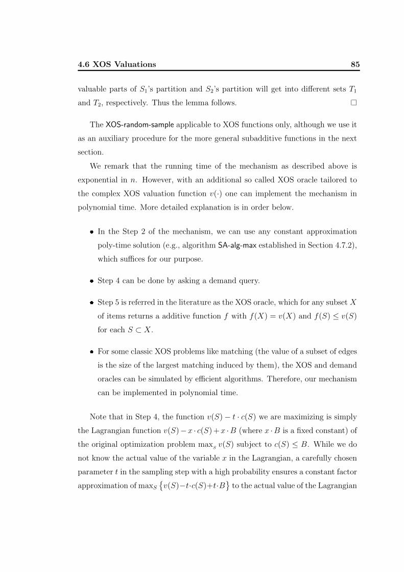
4.6 XOS Valuations 85
valuable parts of S1’s partition and S2’s partition will get into different sets T1
and T2, respectively. Thus the lemma follows.
The XOS-random-sample applicable to XOS functions only, although we use it
as an auxiliary procedure for the more general subadditive functions in the next
section.
We remark that the running time of the mechanism as described above is
exponential in n. However, with an additional so called XOS oracle tailored to
the complex XOS valuation function v(·) one can implement the mechanism in
polynomial time. More detailed explanation is in order below.
In the Step 2 of the mechanism, we can use any constant approximation
poly-time solution (e.g., algorithm SA-alg-max established in Section 4.7.2),
which suffices for our purpose.
Step 4 can be done by asking a demand query.
Step 5 is referred in the literature as the XOS oracle, which for any subset X
of items returns a additive function f with f(X) = v(X) and f(S) ≤ v(S)
for each S ⊂ X.
For some classic XOS problems like matching (the value of a subset of edges
is the size of the largest matching induced by them), the XOS and demand
oracles can be simulated by efficient algorithms. Therefore, our mechanism
can be implemented in polynomial time.
Note that in Step 4, the function v(S)− t · c(S) we are maximizing is simply
the Lagrangian function v(S)−x · c(S) +x ·B (where x ·B is a fixed constant) of
the original optimization problem maxSv(S) subject to c(S) ≤ B. While we do
not know the actual value of the variable x in the Lagrangian, a carefully chosen
parameter t in the sampling step with a high probability ensures a constant factor
approximation of maxSv(S)−t·c(S)+t·B
to the actual value of the Lagrangian

86 Chapter 4. Budget Feasible Mechanism Design 1: Basic Model
maxSv(S)−x ·c(S)+x ·B
and related optimum value v(opt(A)) of the original
problem maxS v(S) subjected to c(S) ≤ B.
The linearity of the Lagrangian, together with the subadditivity of v(·), is
important for us in order to derive the following observations on the threshold t,
subset S∗, and additive function f that were defined in the XOS-random-sample.
Claim 2. For any S ⊆ S∗, f(S)− t · c(S) ≥ 0.
Proof. Assume by contradiction that there exists a subset S ⊆ S∗ such that
f(S) − t · c(S) < 0. Let S ′ = S∗ \ S. Since f is an additive function, we have
c(S ′) + c(S) = c(S∗) and f(S ′) + f(S) = f(S ′ ∪ S) = f(S∗) = v(S∗). Thus,
v(S ′)− t · c(S ′) ≥ f(S ′)− t · c(S ′)
= v(S∗)− t · c(S∗)−(f(S)− t · c(S)
)> v(S∗)− t · c(S∗),
which contradicts the definition of S∗.
The following claim states that any item in S∗ cannot change S∗ by bidding
smaller than his true cost. This fact is crucial for monotonicity and truthfulness
of the mechanism.
Claim 3. If any item j ∈ S∗ reports a smaller cost b(j) < c(j), then set S∗
remains the same.
Proof. Let b be the bid vector where j reports b(j) and other bids remain
unchanged. First we notice that for any set S with j ∈ S,(v(S) − t · b(S)
)−(
v(S)− t · c(S))
= t(c(j)− b(j)
)is a fixed positive value. Hence,
v(S∗)− t · b(S∗) = v(S∗)− t · c(S∗) + t(c(j)− b(j)
)≥ v(S)− t · c(S) + t
(c(j)− b(j)
)= v(S)− t · b(S).

4.6 XOS Valuations 87
Further, for any set S with j /∈ S, we have
v(S∗)− t · b(S∗) > v(S∗)− t · c(S∗)
≥ v(S)− t · c(S)
= v(S)− t · b(S).
Therefore, we conclude that S∗ = argmaxS⊆A\T
(v(S) − t · b(S)
); and by the fixed
tie-breaking rule, S∗ is selected as well.
Our main mechanism for XOS functions is simply a uniform distribution of
the mechanism XOS-random-sample and one that picks the most valuable item.
XOS-mechanism-main
With probability 0.5 run XOS-random-sample.
With probability 0.5 pick item from argmaxi v(i) and pay B.
Theorem 17. The mechanism XOS-mechanism-main is budget feasible and truth-
ful, and provides a constant approximation ratio for XOS valuation functions.
Proof. The proof follows from the following three lemmas.
Lemma 12. XOS-mechanism-main is universally truthful.
Proof. At a high level point of view, our mechanism is built on the idea introduced
in [1] of composing a few different selection rules. In particular, the Steps (1-
4) comprise the first round of selection for winning agents and the Steps (5-7)
further sift out survived agents in the second round. It was shown in [1] that
if the first selection rule is composable (i.e., monotone and in addition to that
any winner cannot manipulate the winning set without losing) and the second
selection rule is just monotone, then their composition is monotone. In our case,
Claim 3 implies the composability of the Steps (1-4) and the monotonicity of
the Steps (5-7) simply follows from the truthfulness of Additive-mechanism. We

88 Chapter 4. Budget Feasible Mechanism Design 1: Basic Model
note that in a single parameter domain monotone allocation rule with threshold
payments implies truthfulness. Therefore, our mechanism is truthful.
Lemma 13. XOS-mechanism-main is budget feasible.
Proof. It suffices to prove that both mechanisms are budget feasible. Clearly,
picking the largest item is budget feasible. XOS-random-sample uses a budget
feasible mechanism Additive-mechanism to decide the final winning set and pay-
ments. Therefore, the threshold payments in XOS-random-sample (the minimum
over all middle steps) can be only smaller than those in Additive-mechanism; this
implies that that XOS-random-sample is budget feasible as well.
Lemma 14. XOS-mechanism-main has a constant approximation ratio.
Proof. Let opt = opt(A) denote the optimal winning set given budget B, and let
k = mini∈optv(opt)v(i)
. Thus v(opt) ≥ k ·v(i) for each i ∈ opt. By Lemma 11, we have
v(opt∩T ) ≥ k−14kv(opt) with probability at least 1
2. Thus, we have v(opt(T )) ≥
v(opt∩T ) ≥ k−14kv(opt) with probability at least 1
2(the first inequality holds
opt∩T is a particular solution and opt(T ) is an optimal solution for set T with
budget constraint).
We let opt∗ = optf (S∗) be the optimal solution with respect to the item set
S∗, additive value-function f and budget B. Below we show that f(opt∗) is a
good approximation to the actual social optimum v(opt). Consider the following
two cases:
c(S∗) > B. With such assumption, we can always find a subset S ′ ⊆ S∗,
such that B2≤ c(S ′) ≤ B. By Claim 2, we know f(S ′) ≥ t · c(S ′) ≥
v(opt(T ))8B
· B2≥ v(opt(T ))
16. Then by the fact that opt∗ is an optimal solution
and S ′ is a particular solution with budget constraint B, we have f(opt∗) ≥f(S ′) ≥ v(opt(T ))
16≥ k−1
64kv(opt) with probability at least 1
2.
c(S∗) ≤ B. Then opt∗ = S∗. Let S ′ = opt \T ; thus, c(S ′) ≤ c(opt) ≤ B. By
Lemma 11, we have v(S ′) ≥ k−14kv(opt) with probability at least 1
2. Recall

4.7 Subadditive Valuations 89
that S∗ = argmaxS⊆A\T
(v(S) − t · c(S)). Then with probability at least 12, we
have
f(opt∗) = f(S∗) = v(S∗)
≥ v(S∗)− t · c(S∗)
≥ v(S ′)− t · c(S ′)
≥ k − 1
4kv(opt)− v(opt(T ))
8B·B
≥ k − 1
4kv(opt)− v(opt)
8
=k − 2
8kv(opt).
In either case, we get
f(opt∗) ≥ min
k − 1
64kv(opt),
k − 2
8kv(opt)
≥ k − 2
64kv(opt)
with probability at least 12. At the end we output the result of Additive-
mechanism(f, S∗, B) in the last step of XOS-random-sample. We recall that
Additive-mechanism has approximation factor of at most 3 with respect to the
optimal solution f(opt∗). Thus the value of the solution given by XOS-random-
sample is at least 13· f(opt∗) ≥ 1
3· 1
2· k−2
64kv(opt) = k−2
384kv(opt).
On the other hand, since k = mini∈optv(opt)v(i)
, the solution given by picking
the largest item satisfies maxi v(i) ≥ 1kv(opt). Combining the two mechanisms
together, our main mechanism XOS-mechanism-main has performance at least(1
2· k − 2
384k+
1
2· 1
k
)v(opt) =
k + 382
768kv(opt) ≥ 1
768v(opt).
This completes the proof of the theorem.
4.7 Subadditive Valuations
We first apply the following straightforward approach, where one simply sub-
stitutes a given general subadditive valuation by its approximation with XOS

90 Chapter 4. Budget Feasible Mechanism Design 1: Basic Model
function. Noticeably, that change in the objective valuation does not cause any
problems with agents’ incentives and thus can be addressed from purely appro-
ximation point of view.
4.7.1 Mechanism via Reduction to XOS
XOS valuations may be equivalently characterized as the class of fractionally
subadditive functions, as was shown in [34]. Let S1, . . . , SN be the tuple of all
possible subsets of A, where N = |2A| is the size of the power set 2A. In particular,
we may consider the following linear program LP(S) for a subset S ⊆ A, where
every subset Sj is associated with a variable αj.
LP (S) : minN∑j=1
αj · v(Sj) (♦)
s.t. αj ≥ 0, 1 ≤ j ≤ N∑j: i∈Sj
αj ≥ 1, ∀ i ∈ S
In (♦) the minimum is taken over all possible non-negative values of α =
(α1, . . . , αN). If we consider each αj as the fraction of the cover by subset Sj,
the last constraint implies that all items in S are fractionally covered. Hence,
LP(S) describes a linear program for the set cover of S. By definition, any
fractionally subadditive function v(·) must obey the inequality v(A′) ≤ LP (A′)
for each A′ ⊂ A.
The above LP has a strong connection to the core of cost sharing games (con-
sidering v(·) instead as a cost function), which is a central notion in cooperative
game theory [60]. Roughly speaking, the core of a game is a stable coopera-
tion among all agents to share v(A) where no subset of agents can benefit by
breaking away from the grand coalition. It is well known that the cores of many
cost sharing games are empty. This motivates the notion of α-approximate core,

4.7 Subadditive Valuations 91
which requires all the agents to share only an α-fraction of v(A). Bondareva-
Shapley Theorem [13, 62] says that for subadditive functions, the largest value α
for which the α-approximate core is nonempty is equal to the integrality gap of
the LP. Further, the integrality gap of the LP equals to one (i.e., v(A) is also an
optimal fractional solution) if and only if the valuation function is XOS, which is
also equivalent to the non-emptiness of the core.
For any subadditive function v(·), it can be seen that the value of the
optimal integral solution to the above LP(S) is always v(S). Indeed, one has
S ⊆⋃j: αj≥1 Sj and
∑j αj · v(Sj) ≥
∑j: αj≥1 v(Sj) ≥ v
(⋃j: αj≥1 Sj
)≥ v(S).
Definition 6. Let v(S) be the value of the optimal fractional solution to LP(S),
and I(S) = v(S)/v(S) be the integrality gap of LP(S). Let I = maxS⊆A I(S).
The integrality gap I gives a worst-case upper bound on the integrality gap
of all subsets. Hence, we have v(S)I ≤ v(S) ≤ v(S) for any S ⊆ A.
The classic Bondareva-Shapley Theorem [13, 62] says that the integrality gap
I(S) is one (i.e., v(S) is also an optimal fractional solution to the LP) if and only
if v(·) is an XOS function.
Lemma 15. v(·) is an XOS function.
Proof. For any subset S ⊆ A, consider any non-negative vector γ = (γ1, . . . , γN) ≥0 that satisfies
∑j: i∈Sj γj ≥ 1 for any i ∈ S. Then we have
N∑j=1
γj · v(Sj) =N∑j=1
γj · minβj,·≥0
N∑k=1
βj,k · v(Sk)
∣∣∣∣∣∣ ∀ i ∈ Sj ,∑
k: i∈Sk
βj,k ≥ 1
= min
β≥0
N∑j=1
γj
N∑k=1
βj,k · v(Sk)
∣∣∣∣∣∣ ∀ j,∀ i ∈ Sj ,∑
k: i∈Sk
βj,k ≥ 1
= min
β≥0
N∑k=1
( N∑j=1
γjβj,k
)· v(Sk)
∣∣∣∣∣∣ ∀ j,∀ i ∈ Sj ,∑
k: i∈Sk
βj,k ≥ 1
≥ min
α≥0
N∑k=1
αk · v(Sk)
∣∣∣∣∣∣ ∀ i ∈ S,∑
k: i∈Sk
αk ≥ 1
= v(S).

92 Chapter 4. Budget Feasible Mechanism Design 1: Basic Model
The inequality above follows from the fact that for any i ∈ S,∑k: i∈Sk
∑j
γjβj,k =∑j
γj∑
k: i∈Sk
βj,k
≥∑j
γj ≥∑j: i∈Sj
γj ≥ 1.
Hence, v(·) is fractionally subadditive, which is equivalent to XOS.
We are now ready to present our first mechanism for subadditive functions.
SA-mechanism-main
1. For each subset S ⊆ A, compute v(S).
2. Run XOS-mechanism-main on the same instance w.r.t. v(·).
3. Output the result of XOS-mechanism-main.
Theorem 18. The mechanism SA-mechanism-main is budget feasible, truthful,
and provides an approximation ratio of O(I) for subadditive functions, where Iis the largest integrality gap of LP(S) for all S ⊂ A.
Proof. Note that the valuation v(·) is a public knowledge and utilities of agents do
not depend on v(·); thus computing v(·) and running XOS-mechanism-main with
respect to v(·) do not affect truthfulness. The claim then follows from Theorem 17
and the fact that v(S)I ≤ v(S) ≤ v(S) for any S ⊆ A (i.e., using v(·) instead of
v(·) we lose at most factor of I in the approximation ratio).
In general, the approximation ratio of the mechanism can be as large as
Θ(log n) [28, 12]. But for those instances when the integrality gap of (♦)
is bounded by a constant (e.g., facility location [60]), our mechanism gives a
constant approximation.

4.7 Subadditive Valuations 93
4.7.2 Sub-Logarithmic Approximation
Subadditive Maximization with Budget We first give an algorithm that
approximates maxS⊆A v(S) given that c(S) ≤ B. That is, we ignore for a while
strategic behaviors of the agents and consider a pure optimization problem.
Dobzinski et al. [30] considered the same question and gave a 4-approximation
algorithm for the unweighted case (i.e., the restriction is on the size of selected
subset). Our next algorithm extends this result to the weighted case and runs
in polynomial time using the demand oracle. Later, Badanidiyuru et al. [6]
gave a 2 + ε approximation polynomial time algorithm to the same weighted
problem that also exploits demand oracle. To make the exposition of this thesis
complete we present below our algorithm, although we admit that in terms of the
approximation ratio it is better to use the algorithm from [6].
SA-alg-max
Let v∗ = maxi∈A v(i) and V = v∗, 2v∗, . . . , nv∗
For each v ∈ V
– ∀i ∈ A set p(i) = v·c(i)2B , find T ∈ argmax
S⊆A
(v(S)−
∑i∈S
p(i)
).
– Let Sv = ∅.
– If v(T ) < v2, then continue to next v.
– Else, in decreasing order of c(i) put items from T in Sv
while preserving budget constraint.
Output: Sv with the largest value v(Sv) for all v ∈ V.
Lemma 16. SA-alg-max is an 8-approximation algorithm for subadditive maxi-
mization with budget working in polynomial time with a demand oracle.
Proof. Let S∗ be an optimal solution. Note that v(S∗) ≥ v∗ = maxi∈A v(i) and
c(S∗) ≤ B. For all v ≤ v(S∗), we first prove that the algorithm will generate a

94 Chapter 4. Budget Feasible Mechanism Design 1: Basic Model
non-empty set Sv with v(Sv) ≥ v4. Since T is the maximum set returned by the
oracle, we have
v(T )− v
2Bc(T ) ≥ v(S∗)− v
2Bc(S∗) ≥ v − v
2B·B ≥ v
2.
Hence, v(T ) ≥ v2. If c(T ) ≤ B, then Sv = T and we are done. Otherwise,
by the greedy procedure of picking items from T to Sv, we are guaranteed that
c(Sv) ≥ B2
. Assume for contradiction that v(Sv) <v4. Then
v(T \ Sv)−v
2Bc(T \ Sv) ≥ v(T )− v(Sv)−
v
2B
(c(T )− c(Sv)
)> v(T )− v
4− v
2Bc(T ) +
v
2B· B
2
= v(T )− v
2Bc(T ).
The latter contradicts the definition of T , since T \ Sv is then better than T .
Thus, we always have v(Sv) ≥ v4
for each v ≤ v(S∗). Since the algorithm tries
all possible v ∈ V (including one with v(S∗)2
< v ≤ v(S∗)) and outputs the largest
v(Sv), the output is guaranteed to be within a factor of 8 to the optimal value
v(S∗).
Remark 2. Note that we can actually modify the algorithm to get a (4 + ε)-
approximation with running time polynomial in n and 1ε. To do so one may simply
replace V by a larger setεv∗, 2εv∗, . . . , dn
εeεv∗
. Both algorithms suffice for our
purpose; for the rest of the paper, for simplicity we will use the 8-approximation
algorithm, to avoid the extra parameter ε in the description.
We will use SA-alg-max further as a subroutine in the mechanism SA-random-
sample. When there are different sets maximizing v(S) −∑
i∈S p(i), we require
that the demand query oracle always returns a fixed set T . This property
is important for truthfulness of our mechanism. To implement this, we set
some fixed order on the items i1 ≺ i2 ≺ · · · ≺ in. We first compute T1 ∈argmaxS⊆A
(v(S)−
∑i∈S
p(i))
and T2 ∈ argmaxS⊆A\i1(v(S)−
∑i∈S
p(i)). If v(T1)−∑
i∈T1 p(i) = v(T2) −∑
i∈T2 p(i), we know that there is a subset without i1

4.7 Subadditive Valuations 95
that gives us the maximum; thus, we ignore i1 for further consideration. If
v(T1)−∑
i∈T1 p(i) > v(T2)−∑
i∈T2 p(i), we know that i1 should be in any optimal
solution; hence, we keep i1 and proceed the process iteratively for i2, i3, . . . , in.
This process clearly gives a fixed outcome that maximizes v(S)−∑
i∈S p(i).
We present now another mechanism for subadditive valuation based on the
ideas of random sampling and cost sharing. In contrast to the previous SA-
mechanism-main this procedure runs in polynomial time and has an o(log n)
approximation ratio, which improves upon previously best known ratio [30] of
O(log2 n).
Let us first consider the following mechanism, based on random sampling and
cost sharing.
SA-random-sample
1. Sample items independently at random with probability 12
in group T.
2. Run SA-alg-max on the item set T, let v be the value of
the returned set.
3. For k = 1 to |A \ T |
Run SA-alg-max on the item seti ∈ A \ T | c(i) ≤ B
k
,
where each item has cost Bk , denote output by X.
If v(X) ≥ log logn80 logn · v
– Output X, pay Bk to each item in X.
– Halt.
4. Output ∅.
In the above mechanism, we again first sample half in expectation of the items
to form a testing group T , and then use SA-alg-max to compute an approximate
solution for the items in T given the budget constraint B. As it can be seen in

96 Chapter 4. Budget Feasible Mechanism Design 1: Basic Model
the analysis of the mechanism, the computed value v is (in expectation) within
a constant factor of the optimal value of the whole set A. That is, we are able
to learn the rough value of the optimal solution by random sampling. Next we
consider the remaining items A \ T and try to find a subset X with a relatively
big value in which every item is willing to “share” the budget B at a fixed share
Bk
. (This part of our mechanism can be viewed as a reversion of the classic cost
sharing mechanism.) Finally, we use the information v from the sample as a
benchmark to determine whether X should be a winning set or not.
Finally, the mechanism for subadditive functions is as follows.
SA-mechanism-main-2
With probability 0.5, run SA-random-sample.
With probability 0.5, pick item from argmaxi v(i) and pay B
Theorem 19. SA-mechanism-main-2 runs in polynomial time, given a demand
oracle, and it is a truthful budget feasible mechanism for subadditive functions
with an approximation ratio of O( lognlog logn
).
Proof. Let S = A \ T . It is obvious that the mechanism runs in polynomial
time since SA-alg-max works in polynomial time. When the mechanism picks the
largest item, it is certainly budget feasible, as the total payment is precisely B.
If it chooses SA-random-sample, either no item is a winner or X is selected as the
winning set. Note that |X| ≤ k and each item in X gets a payment of Bk
. It is
therefore budget feasible as well.
(Truthfulness.) Truthfulness for the part of picking the largest item is obvious,
as the outcome is irrelevant to the submitted bids. Next we prove that SA-
random-sample is truthful as well. The random sampling step does not depend
on the item’s bids, and items in T have no incentive to lie as they cannot win
anyway. Hence, it suffices to consider only items in S. We observe that every
agent becomes a candidate to win only if c(i) ≤ Bk
. Consider any item i ∈ S and

4.7 Subadditive Valuations 97
fix bids of other items. If i reports his true cost c(i), there are the following three
possibilities.
Item i wins and is paid Bk
. Then c(i) ≤ Bk
and his utility is Bk− c(i) ≥ 0. If
i reports a bid which is still less than or equal to Bk
, the output and all the
payments do not change. If i reports a bid which is larger than Bk
, he still
could not win for a share larger than Bk
and will not be considered for all
smaller shares. Therefore, he derives 0 utility. Thus for either case, i does
not have incentive to lie.
Item i loses, and the payment to each winner is Bk≥ c(i). In this case, if i
reduces or increases his bid, he cannot change the output of the mechanism.
Thus i always has zero utility.
Item i loses, and the payment to each winner is Bk< c(i), or the winning
set is empty. In this case, if i reduces his bid, he will not change the process
of the mechanism until the payment offered by the mechanism is less than
c(i). Thus, even if i could win for some value k, the payment he gets would
be less than c(i), in which case his utility is negative. If i increases his bid,
he loses and thus derives zero utility.
Therefore, SA-random-sample is a universally truthful mechanism.
(Approximation Ratio.) It remains to estimate the approximation ratio. Let
opt = opt(A) denote the optimal solution for the whole set.
If there exists an item i ∈ A such that v(i) ≥ 12v(opt), then picking the largest
item will generate the value at least 12v(opt) and we are done. Below we assume
that v(i) < 12v(opt) for all i ∈ A. Then, by Lemma 11, with probability at least 1
2
we have v(opt(T )) ≥ 18v(opt) and v(opt(S)) ≥ 1
8v(opt). Hence, with probability
at least 14
we have
v(opt(S)) ≥ v(opt(T )) ≥ 1
8v(opt). (4.5)

98 Chapter 4. Budget Feasible Mechanism Design 1: Basic Model
Therefore, it suffices to prove that the main mechanism has an approximation
ratio of O( lognlog logn
) given the inequalities (4.5).
Since SA-alg-max is an 8-approximation of v(opt(T )), we have v ≥ 18v(opt(T )) ≥
164v(opt). Clearly, if SA-random-sample outputs a non-empty set, then its value
is at least log logn80 logn
· v ≥ log logn5120 logn
· v(opt). Hence, it remains to prove that the
mechanism will always output a non-empty set given formula (4.5).
Let S∗ = 1, 2, 3, . . . ,m ⊆ S be an optimal solution of S, given the budget
constraint B and c1 ≥ c2 ≥ · · · ≥ cm. We recursively divide the agents in S∗ into
different groups as follows:
Let α1 be the largest integer such that c1 ≤ Bα1
. Put the first minα1,magents into group Z1.
Let βr = α1 + · · ·+ αr. If βr < m let αr+1 be the largest integer such that
cβr+1≤ B
αr+1; put the next minαr+1,m− βr agents into group Zr+1.
Let us denote by x+1 the number of groups. Since the items in S∗ are ordered
by c1 ≥ c2 ≥ · · · ≥ cm, we have αr+1 ≥ αr for any r. If there exists a set Zj such
that v(Zj) ≥ log logn10 logn
· v, then the mechanism outputs a non-empty set, as it could
buy αj items at price Bαj
given that SA-alg-max is an 8-approximation and the
threshold we set is v(Zj) ≥ log logn80 logn
·v. Thus, we may assume that v(Zj) <log logn10 logn
·vfor each j = 1, 2, . . . , x+ 1. On the other hand, by subadditivity, we have
x+1∑j=1
v(Zj) ≥ v(S∗) = v(opt(S)) ≥ v(opt(T )) ≥ v.
Putting the two inequalities together, we can conclude that (x+1) · log logn10 logn
·v > v,
which implies that
x >5 log n
log log n≥ 5 logm
log logm.
On the other hand, since S∗ = 1, 2, 3, . . . ,m is a solution for S within the
budget constraint, we have that∑m
j=1 cj ≤ B. Further, since c1 >B
α1+1, c
β1+1>

4.7 Subadditive Valuations 99
Bα2+1
, . . . , cβx+1
> Bαx+1+1
, we have
B ≥m∑j=1
cj ≥ c1 + α1cβ1+1+ · · ·+ αxcβx+1
>B
α1 + 1+
α1B
α2 + 1+ · · ·+ αxB
αx+1 + 1.
Hence,
1 ≥ 1
α1 + 1+
α1
α2 + 1+ · · ·+ αx
αx+1 + 1≥ 1
2α1
+α1
2α2
+ · · ·+ αx2αx+1
.
In particular, we get
2 ≥ 1
α1
+α1
α2
+ · · ·+ αx−1
αx≥ x
x
√1
α1
α1
α2
· · · αx−1
αx,
where the last inequality is simply the inequality of arithmetic and geometric
means. Hence, we get 2 ≥ xx√
1αx
, which is equivalent to αx ≥ (x2)x. Now
plugging in the fact that m ≥ αx and x ≥ 5 logmlog logm
, we come to a contradiction.
This concludes the proof.


Chapter 5Budget Feasible Mechanism Design 2:
Extensions
In this chapter we introduce some natural extensions of the budget feasible model.
First, we analyze the original setup in a more relaxed classical Bayesian framework
as opposed to the former worst-case prior-free framework. Second, we suggest a
generalization of the basic model to the case, where each agent is allowed to have
more than one item for sale.
Bayesian mechanism design. As a standard game theoretic model for in-
complete information, Bayesian mechanism design assumes that agents’ private
information (i.e., (c(i))i∈A in the basic model) is drawn from a known distribution.
In contrast to the previous chapter, if we have prior knowledge about the cost’s
distribution, then we can obtain more positive results in the form of constant
approximation truthful mechanisms. It turns out that the question
“A fundamental question is whether, regardless of computational con-
straints, a constant-factor budget feasible mechanism exists for subad-
ditive functions,”
posed by Dobzinski, Papadimitriou, Singer in [30] has an affirmative answer.
101

102 Chapter 5. Budget Feasible Mechanism Design 2: Extensions
Techniques. The major approach in the design of budget feasible mechanisms
for additive and submodular valuations is based on a simple idea of adding agents
one by one greedily and carefully ensuring that the budget constraint is not
violated. All mechanisms in this thesis for XOS and subadditive valuations, from
a high level structural point of view, use a different approach of random sampling.
In the Bayesian setting, random sampling is often deemed to be unnecessary,
because, when we have knowledge of the distribution, it is tempting to use a ‘prior
sampling’ approach to generate random virtual instances, and based on them get
an estimate for the real instance. While this works well when the private costs
c(i) of every agent are drawn independently, interestingly (and surprisingly), it
fails when costs c(i)’s are correlated in the distribution. We therefore still have to
use “real” random sample to get a rough estimate based on the sampled test set;
the collected information from random sampling correctly reflects the structure
of the private costs (with a high probability) even for correlated distributions.
Random sampling appears to be a powerful tool in mechanism design and
has been used successfully in other domains such as digital goods auctions [39],
secretary problem [5, 4], social welfare maximization [28], and mechanism design
without money [20].
Multi-parameter. The design of mechanisms for agents having a rich multi-
parameter bidding language is known to be much harder than for the scenarios
where each agent provides only a single real number. Indeed, the restrictions
on what auctioneer can choose as an outcome and payments become much more
complicated than the threshold rule we were using so far in the scenario with
single-item sellers. Generally speaking, in a multi-parameter case there is no such
simple characteristic property for a mechanism being incentive compatible as the
one of monotonicity in the single parameter domains [52, 3]. Not surprisingly,
there are considerably fewer positive results in the multi-parameter settings than
in the single-parameter settings. Thus it is quite unexpected to see a truthful
mechanism with good performance guarantees in the multi-parameter extension

5.1 Bayesian Framework 103
of the original budget feasible model.
5.1 Bayesian Framework
In this section we study budget feasible mechanisms for subadditive functions
from a standard economic viewpoint, where the costs of all agents (c(i))i∈A are
drawn from given distribution D. More specifically, the mechanism designer and
all participants know in advance D, from which the real cost vector (c(i))i∈A is
drawn. However, each c(i) is the private information of agent i. Distribution Dis given on the probability space Ω with the corresponding density function ρ(·)on R|A|. We allow dependencies on the agents’ costs in D. We need some mild
technical restriction on D in order to sample a conditioned random variable. We
assume that the density function ρ(·) of D is integrable over each subset S ⊆ A
of its variables for any choice of the rest parameters, i.e., ρ(cA\S) =∫
Ωρ(c) dxS
is bounded. This condition is reminiscent of integrability of marginal density
functions (see, e.g., page 331 of [65]), though in our case we require a slightly
stronger condition. This includes independent distributions as a special case.
We note that any distribution with discrete and finite support satisfies this
requirement.
Every agent submits a bid b(i) and seeks to maximize his own utility. We
again consider universally truthful mechanisms, i.e., for every coin flip of the
mechanism and each cost vector, truth-telling is a dominant strategy for every
agent.
The performance of a mechanism M is measured now in expectation by
E[M] = Ec∼D[M(c)].
It is compared to the expected value of the optimal solution, given by
E[opt] = Ec∼D[v(opt(c))
].
We say mechanism M is a (Bayesian) α-approximation if E[opt]E[M]
≤ α.

104 Chapter 5. Budget Feasible Mechanism Design 2: Extensions
Interestingly, in the budget feasible model one does not need to rely on
Bayesian analysis in the following aspects:
Truthfulness. In most of the previous works in Bayesian mechanism design
regarding social welfare maximization, e.g. [45, 10, 44, 16], the considered
solution concept is Bayesian truthfulness, i.e., truth-telling is in expectation
an equilibrium strategy when other agents’ profiles are drawn from the
known distribution. In budget feasible model it is still possible to achieve
universal truthfulness, meaning that truth-telling is dominant strategy of
each agent for any coin flips of the mechanism and any instance of the costs.
Thus universal truthfulness is a stronger solution concept than Bayesian
truthfulness. Universal truthfulness in Bayesian mechanism design has also
been used in, e.g. [15], but with a different focus on profit maximization.
Distribution. Regarding the prior knowledge of the distribution, most of the
previous related works consider independent distributions, e.g. [46, 45, 10,
44]. In the budget feasible model one may still allow general distributions
with a correlation of costs. Dependency on private information is a natural
phenomenon arising in practice and it has been considered for, e.g., auc-
tions [56]. In our model, although costs are private parameters, correlation
among them appears to be common occurrence. For example, if the price
on crude oil goes up, the incurred costs of all agents for producing their
items will go up as well.
In this section we: let optv(c, S) denote the winning set in an optimal solution
with the valuation function v(·), the cost vector is c, and the agent set is S (the
parameters are omitted if they are clear from the context); let v(optv(c, S)) denote
the value of optv(c, S).
We present below a Bayesian constant approximation universally truthful
mechanism for a general subadditive valuation v(·). We note that this mechanism
does not always work in polynomial time.
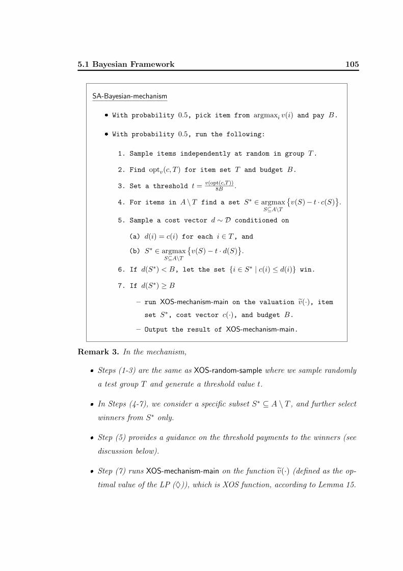
5.1 Bayesian Framework 105
SA-Bayesian-mechanism
With probability 0.5, pick item from argmaxi v(i) and pay B.
With probability 0.5, run the following:
1. Sample items independently at random in group T.
2. Find optv(c, T ) for item set T and budget B.
3. Set a threshold t = v(opt(c,T ))8B .
4. For items in A \ T find a set S∗ ∈ argmaxS⊆A\T
v(S)− t · c(S)
.
5. Sample a cost vector d ∼ D conditioned on
(a) d(i) = c(i) for each i ∈ T, and
(b) S∗ ∈ argmaxS⊆A\T
v(S)− t · d(S)
.
6. If d(S∗) < B, let the set i ∈ S∗ | c(i) ≤ d(i) win.
7. If d(S∗) ≥ B
– run XOS-mechanism-main on the valuation v(·), item
set S∗, cost vector c(·), and budget B.
– Output the result of XOS-mechanism-main.
Remark 3. In the mechanism,
Steps (1-3) are the same as XOS-random-sample where we sample randomly
a test group T and generate a threshold value t.
In Steps (4-7), we consider a specific subset S∗ ⊆ A \ T , and further select
winners from S∗ only.
Step (5) provides a guidance on the threshold payments to the winners (see
discussion below).
Step (7) runs XOS-mechanism-main on the function v(·) (defined as the op-
timal value of the LP (♦)), which is XOS function, according to Lemma 15.

106 Chapter 5. Budget Feasible Mechanism Design 2: Extensions
Further remarks about the mechanism are in order.
It is tempting to remove the random sampling part, as given D one may
consider a ‘prior sampling’ approach: Generate some virtual instances ac-
cording to D and compute a threshold t based on them; then apply this
threshold to all agents in A. Interestingly, the prior sampling approach
works well in our mechanism for, e.g., the case when all c(i)’s are indepen-
dent, but it does not work for the case when variables are dependent.
For instance, consider additive valuation v(S) = |S|, budget B = 2k for a
large k, and a set of N = 2k agents with the following discrete distribution
over costs (c = ` means that c(i) = ` for all i):
Pr[c = 1] =1
2k+1,Pr[c = 2] =
1
2k, . . . ,
Pr[c = 2k
]=
1
2,Pr
[c = 2k+1
]=
1
2k+1.
Note that
v(opt(c = 1)) = 2k, v(opt(c = 2)) = 2k−1, . . . . . . ,
v(
opt(c = 2k
))= 1, v
(opt(c = 2k+1
))= 0.
The expected optimal value is E[opt] = k+12
and it is equally spread over
all possible costs except the last one c = 2k+1. Roughly speaking, on a
given instance c, any prior estimate on v(opt(c)) that gives a constant
approximation only applies to a constant number of distinct costs (the
contribution of these cases to E[opt] is negligible). Hence for the rest almost
all possible costs, we get a meaningless estimate for opt(c). Therefore, the
prior sampling will lead to a bad approximation ratio.
Why do we generate another cost vector d in Step (5)? Recall that
our target winner set is S∗, whose value v(S∗) in expectation gives a
constant approximation to E[opt]. However, we face the problems of
selecting a winning set in S∗ of a sufficiently large value and distributing

5.1 Bayesian Framework 107
the budget among the winners. These two problems together are closely
related to cooperative game theory and the notion of approximate core.
For subadditive valuations, a constant approximate core may not exist [60]
(e.g., set cover provides a logarithmic lower bound [12]). Thus we might
not be able to pick a winning set with a constant approximation and set
threshold payments in accordance with the valuation function. The question
then is: is there any other guidance we can take to bound budget feasible
threshold payments and give a constant approximation?
Our solution is to use another random vector d that serves as such a
guidance. (Conditions in Steps (5a) and (5b), from a high level point of
view, guarantee that the vector d is not too ‘far’ from c for the agents in S∗,
in the sense that both vectors are derived from the same distribution. Thus,
cost vectors c and d are distributed symmetrically and can be switched while
preserving some important parameters such as t and S∗ in expectation.) If
d(S∗) ≤ B (Step (6)), then we set d(i) as an upper bound on the payment
of each agent i ∈ S∗; this guarantees that we are always within the budget
constraint. If d(S∗) > B, setting d(i) as an upper bound is not sufficient
to ensure budget feasibility; then we adopt our approach for XOS functions
with inputs subset S∗ and XOS valuation v(·) defined by (♦).
Theorem 20. SA-Bayesian-mechanism is a universally truthful budget feasible
mechanism for subadditive functions and gives in expectation a constant appro-
ximation.
Proof. Budget feasibility follows simply from the description of the mechanism
and the fact that XOS-mechanism-main is budget feasible.
For universal truthfulness, we note that in the mechanism, the sampled vector
d comes from a distribution that depends on actual bid vector c. To see why our
mechanism takes a distribution over deterministic truthful mechanisms, we can
describe all possible samples d for (i) all possible cost vectors on T and (ii) all
possible choices S ⊆ A \ T of S∗; then we tell all flipped d’s to the agents before

108 Chapter 5. Budget Feasible Mechanism Design 2: Extensions
looking at the costs of T . (Practically, we can provide all our randomness as a
black box accessible by all agents.) Note that the selection rule of S∗ is monotone,
and, similarly to Claim 3, each agent in S∗ cannot manipulate (i) the composition
of S∗ given c and T , and (ii) the choice of d, as long as he stays in S∗. Therefore,
composing the first part choosing S∗ (Step (4)) with the next monotone rule
picking winners in S∗ (Steps (6-7)), we again get a monotone winner selection
rule. Hence, the mechanism is universally truthful.
Next we give a sketch of the idea of proving the constant approximation.
Approximation analysis (sketch). We sketch the proof idea of the approximation
ratio of the mechanism. Later in section 5.1.1 we give a complete argument.
First, similar to our analysis in Section 4.6, the optimal solution v(opt(c, T ))
obtained from random sampling in expectation gives a constant approximation
to the optimal solution E[opt]. Further, we observe the following facts (which are
reminiscent of Claim 2):
v(S)− t · c(S) ≥ 0 and v(S)− t · d(S) ≥ 0, ∀S ⊆ S∗
where the second inequality is based on the conditional distribution we choose
for d.
If c(S∗) ≥ B and d(S∗) ≥ B (i.e., the mechanism runs Step (7)), we can pick
a subset S0 ⊆ S∗ with B ≥ c(S0) ≥ B2
. By Theorem 17 XOS-mechanism-main
gives a constant approximation to the optimum of v(·) on S∗. (This is the reason
why in Step (7) of the mechanism, we run the whole XOS-mechanism-main on the
input instance v(·) and S∗.) Hence,
v(optv(c, S∗)) ≥ v(S0) ≥ t · c(S0) ≥ t · B
2≥ v(opt(c, T ))
16,
where the first inequality follows from the fact that S0 ⊆ S∗ is a budget feasible
set. Thus, the optimum of v(·) on S∗ is within a constant factor of v(opt(c, T )),
as well as the benchmark E[opt].
If c(S∗) < B and d(S∗) ≥ B, we have v(S∗) ≥ t · d(S∗) ≥ v(opt(c,T ))8
. Further,

5.1 Bayesian Framework 109
we notice that S∗ is budget feasible with respect to cost vector c; thus, XOS-
mechanism-main gives a constant approximation to v(S∗), which in turn is within
a constant factor of v(opt(c, T )) and E[opt].
We observe that the vectors d and c restricted to the agents in S∗ and
conditioned on
S∗ ∈ argmaxS⊆A\T
v(S)− t · d(S)
, S∗ ∈ argmax
S⊆A\T
v(S)− t · c(S)
have exactly the same distributions. Therefore, due to such a symmetry between
d and c, in a run of our mechanism in expectation we will have the outcome
T, t, S∗ and a pair of vectors (c, d) equally often as the outcome T, t, S∗ and the
pair (d, c). This implies that in the case when d(S∗) < B and c(S∗) < B, we
get on average the value of at least 12v(S∗), since the winning sets on the two
instances where c (resp., d) is the private cost and d (resp., c) is the sampled cost
altogether cover S∗, and v is a subadditive function. By the choice of threshold
t, we also know that
v(S∗) ≥ v(S∗)− t · c(S∗)
≥ v(opt(c, A \ T ))− t · c(opt(c, A \ T ))
≥ v(opt(c, A \ T ))− t ·B.
Thus, our mechanism gives a constant approximation to v(opt(c)) with some
constant probability.
The last case is when c(S∗) ≥ B and d(S∗) < B. Again due to the symmetry
between c and d, intuitively, we can treat this case as the above one when c and d
are switched; thus we also get a constant approximation to E[opt]. (The formal
argument, however, due to multiple randomness used in the mechanism, is much
more complicated.) Therefore, the mechanism SA-Bayesian-mechanism on average
has a constant approximation to the expected socially optimal value E[opt].

110 Chapter 5. Budget Feasible Mechanism Design 2: Extensions
5.1.1 Approximation Guarantees
Below we provide a formal proof for the constant approximation of SA-Bayesian-
mechanism. We first have the following observation.
Claim 4. For any S ⊆ S∗, v(S)− t · c(S) ≥ 0.
Proof. Indeed, recall that S∗ = arg maxS⊆A\T
v(S)−t·c(S)
. Then v(S)−t·c(S) ≥ 0
for any S ⊆ S∗, since otherwise, we have v(S)− t · c(S) < 0 for some S ⊆ S∗ and
we get
v(S∗ \ S)− t · c(S∗ \ S) ≥ v(S∗)− v(S)− t · c(S∗ \ S)
= v(S∗)− t · c(S∗)−(v(S)− t · c(S)
)> v(S∗)− t · c(S∗),
a contradiction.
Thus, for any S ⊆ S∗, v(S) ≥ t · c(S). Therefore, in the description of LP (S),
we have v(Sj) ≥ t · c(Sj) for each j ∈ [1, N ]. Now substituting v(Sj) for c(Sj) in
LP (S), we get the desired inequality v(S) = LP (S) ≥ t · c(S).
We assume that no single item can have cost more than B in the cost vector
c. We need extra notation. We assume that the distribution D is given on the
probability space Ω with corresponding density function ρ(x) on R|A|. For a set
T ⊆ A, let xT
be a point in R|T |. We will denote by ρ(xT) the distribution’s
density we get on the corresponding space R|T | by sampling x ∈ R|A| from D and
restricting it to T -coordinates of x. By ρ(x|xT) we denote the conditional density
obtained by fixing T -coordinates of x to be the same as in xT. By opt(x, S) we
denote the optimal value we can get from the set S ⊆ A on cost vector x with
budget B. For brevity sometimes we will omit x or S, in the latter case S = A;
sometimes we take the optimum over valuation v instead of v, so to emphasis this
we employ notation optv(x, S). In the mechanism we compute the set S∗(c, T ),
which depends on the sampled set T and cost vector c. By XOS(c, S∗) we denote

5.1 Bayesian Framework 111
the value we get from XOS-mechanism-main(c, S∗) run on the set S∗, cost vector
c and XOS valuation v(·) that alone depends on v(·).
In the following we write explicitly the expected value of the second part of
our mechanism.
∫Ω
1
2|A|
∑T⊂A
∫Ω
f(x, y, T )ρ(y∣∣∣y = x |
T;S∗(x, T ) = S∗(y, T )
)dyρ(x)dx, (5.1)
where
f(c, d, T ) =
XOS(c, S∗) if d(S∗) ≥ B
v(S∗ ∩ i : c(i) ≤ d(i)) if d(S∗) < B,
Swapping in (5.1) the sum and integral we get
1
2|A|
∑T⊂A
∫Ω
∫Ω
f(x, y, T )ρ(y∣∣∣y = x |
T;S∗(y, T ) = S∗(x, T )
)dyρ(x)
dx =
1
2|A|
∑T⊂A
∫Ω(T )
∫Ω
∫Ω
f(x, y, T )ρ(y∣∣∣xT ;S∗(y, T ) = S∗(x, T )
)dy
ρ(x∣∣∣xT) dx ρ
(xT
)dx
T=
1
2|A|
∑T⊂A
∫Ω(T )
∫Ω
∑S⊂A\T
∫Ω
f(x, y, T )ρ(y∣∣∣xT ;S∗(y, T ) = S∗(x, T )
)dy
ρ(x∣∣∣xT ;S∗(x, T ) = S
)· Pr
(S∗(x, T ) = S
∣∣∣xT) dx ρ(xT
)dx
T=

112 Chapter 5. Budget Feasible Mechanism Design 2: Extensions
1
2|A|
∑T⊂A
∫Ω(T )
∑S⊂A\T
∫Ω
∫Ω
f(x, y, T )ρ(y∣∣∣xT ;S∗(y, T ) = S
)dy·
ρ(x∣∣∣xT ;S∗(x, T ) = S
)dx
Pr(S∗(·, T ) = S∣∣∣xT) ρ
(xT
)· dx
T=
1
2|A|
∑T⊂A
∫Ω(T )
∑S⊂A\T
∫Ω
∫Ω
f(x, y, T ) + f(y, x, T )
2ρ(y∣∣∣xT ;S∗(y, T ) = S
)dy
ρ(x∣∣∣xT ;S∗(x, T ) = S
)dx Pr
(S∗(·, T ) = S
∣∣∣xT) ρ(xT
)· dx
T.
To get the first equality we split the integral w.r.t. variable x into two integrals
w.r.t. variables xT∈ R|T | and x conditioned on x = x
Ton T ; the second equality
follows from the law of total expectation applied to the variable in the square
brackets with conditioning on all possible values of random variable S∗(·, T )|xT;
to get the third equality we swap integral with the sum; to get the last equality we
have used the symmetry between x and y for the expression in square brackets.
Next, the formula (5.1) can be written as
∫Ω
1
2|A|
∑T⊂A
∫Ω(x,T )
f(x, y, T ) + f(y, x, T )
2
ρ(y∣∣∣y = x |
T;S∗(x, T ) = S∗(y, T )
)dyρ(x)dx, (5.2)
Now we estimate the value of XOS(c, S∗) in the case when d(S∗) ≥ B. Recall
that v(S) ≤ v(S) for any set S ⊆ A. According to the results of previous
section for the XOS functions we have a constant approximation to the optimum:
XOS(c, S∗) ≥ α · v(optv(c, S∗)), for a positive constant α. Now we consider two
cases for c(S∗).
1. c(S∗) < B. Since one can buy the whole set S∗, we have optv(c, S∗) = S∗.
We recall that by definition vector d is sampled so that d(i) = c(i) on
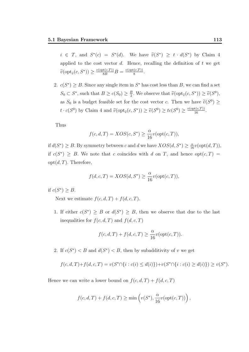
5.1 Bayesian Framework 113
i ∈ T , and S∗(c) = S∗(d). We have v(S∗) ≥ t · d(S∗) by Claim 4
applied to the cost vector d. Hence, recalling the definition of t we get
v(optv(c, S∗)) ≥ v(opt(c,T ))
8BB = v(opt(c,T ))
8.
2. c(S∗) ≥ B. Since any single item in S∗ has cost less than B, we can find a set
S0 ⊂ S∗, such that B ≥ c(S0) ≥ B2. We observe that v(optv(c, S
∗)) ≥ v(S0),
as S0 is a budget feasible set for the cost vector c. Then we have v(S0) ≥t · c(S0) by Claim 4 and v(optv(c, S
∗)) ≥ v(S0) ≥ tc(S0) ≥ v(opt(c,T ))16
.
Thus
f(c, d, T ) = XOS(c, S∗) ≥ α
16v(opt(c, T )),
if d(S∗) ≥ B. By symmetry between c and d we haveXOS(d, S∗) ≥ α16v(opt(d, T )),
if c(S∗) ≥ B. We note that c coincides with d on T , and hence opt(c, T ) =
opt(d, T ). Therefore,
f(d, c, T ) = XOS(d, S∗) ≥ α
16v(opt(c, T )),
if c(S∗) ≥ B.
Next we estimate f(c, d, T ) + f(d, c, T ).
1. If either c(S∗) ≥ B or d(S∗) ≥ B, then we observe that due to the last
inequalities for f(c, d, T ) and f(d, c, T )
f(c, d, T ) + f(d, c, T ) ≥ α
16v(opt(c, T )).
2. If c(S∗) < B and d(S∗) < B, then by subadditivity of v we get
f(c, d, T )+f(d, c, T ) = v(S∗∩i : c(i) ≤ d(i))+v(S∗∩i : c(i) ≥ d(i)) ≥ v(S∗).
Hence we can write a lower bound on f(c, d, T ) + f(d, c, T )
f(c, d, T ) + f(d, c, T ) ≥ min(v(S∗),
α
16v(opt(c, T ))
),

114 Chapter 5. Budget Feasible Mechanism Design 2: Extensions
which does not depend on d. We plug in this lower bound, instead of f(c, d, T ) +
f(d, c, T ), into the formula (5.2). We obtain
∫Ω
1
2|A|
∑T⊂A
∫Ω(x,T )
min(v(S∗), α
16v(opt(x, T ))
)2
ρ(y∣∣∣y = x |
T;S∗(x, T ) = S∗(y, T )
)
dyρ(x)dx =
∫Ω
1
2|A|
∑T⊂A
min
(v(S∗(x, T ))
2,α
32v(opt(x, T ))
)ρ(x)dx.
The equality holds, since y comes from probability distribution and the
function under integral does not depend on y.
Let i∗(x) be the most valuable item in A with c(i∗) ≤ B. We can write the
following lower bound on the total valuation of SA-Bayesian-mechanism.
∫Ω
(0.5× v(i∗(x)) + 0.5× 1
2|A|
∑T⊂A
min
(v(S∗(x, T ))
2,α
32v(opt(x, T ))
))ρ(x)dx.
The optimal expected value is
∫Ω
v(opt(x))ρ(x)dx.
Next we argue that the function
g(x) := v(i∗(x)) +1
2|A|
∑T⊂A
min
(v(S∗(x, T ))
2,α
32v(opt(x, T ))
)approximates v(opt(x)) within a constant factor for any cost vector x.
We fix a cost vector x. Let v(i∗) = 1kv(opt), for some k ≥ 1. We know that
due to the Lemma 11 min (v(opt(A \ T ), v(opt(T ))) ≥ k−14kv(opt) with probability
at least 12. For each “good” T , i.e., such that min (v(opt(A \ T ), v(opt(T ))) ≥
k−14kv(opt), we can write:
v(opt(T )) ≥ k − 1
4kv(opt)

5.1 Bayesian Framework 115
and
v(S∗) ≥ v(S∗)− t · x(S∗) ≥ v(opt(A \ T ))− t · x(opt(A \ T ))
≥ k − 1
4kv(opt)− t ·B ≥ k − 1
4kv(opt)− v(opt)
8B·B
≥ k − 2
8kv(opt).
The second inequality holds because S∗ ∈ arg maxS⊆A\T
v(S) − t · x(S)
; the
third inequality holds because the cost of feasible solution opt(A \ T ) is within
the budget; in the forth inequality we plugged in the definition of t and used the
fact that v(opt) ≥ v(opt(T )).
Therefore, combining these two lower bounds for all “good” T we get
g(x) ≥(
1
k+
1
2min
(k − 2
16k,(k − 1)α
128k
))v(opt(x))
≥ 1
2
(min
(k + 14
16k,kα
128k
))v(opt(x))
≥ α
256v(opt(x)).
Hence, we have shown that the expected value of SA-Bayesian-mechanism is
within a constant factor of α512
from the expected value of the optimal solution.
5.1.2 Back to Prior-free
Finally, we turn back to the original prior-free worst-case framework and based
on the results from Bayesian framework show the existence of budget feasible
incentive compatible mechanism with constant approximation to the optimum
for any subadditive valuation and any bid vector. This settles in the affirmative
the “fundamental question”’ posed by Dobzinski, Papadimitriou, Singer in [30].
Theorem 21. For any given subadditive valuation v(·) and budget B there exists
a budget feasible incentive compatible mechanism with a constant approximation
to the optimum.

116 Chapter 5. Budget Feasible Mechanism Design 2: Extensions
Proof. Let A be the space of all universally truthful budget feasible mechanisms.
Note that A forms a convex set, since for any two mechanisms A1, A2 ∈ Aone may define another universally truthful budget feasible mechanism A =
λ · A1 + (1 − λ) · A2, which with probability λ runs A1 and with probability
1− λ runs A2.
Without loss of generality, we may consider only those situations where every
agent could submit finitely many different numbers as a bid (say all integer
multiples of · B2n
not exceeding B + 1). Note that there are only finitely many
possible allocation rules over the finite space of feasible bids. Therefore, we may
also assume that there are only finitely many deterministic truthful mechanisms
in A. We notice as well that all our integrability assumptions on the prior
distribution in Bayesian framework trivially hold true for any distribution over a
finite set.
We now recall our constant (λ0 > 0) approximation results from Theorem 20
in the Bayesian framework: for any given distribution D of cost vector there is a
mechanism A ∈ A s.t.
Ec∼D[v(A(c))
]≥ λ0 · Ec∼D
[v(opt(c))
].
Let us consider a 2 player game with the first player deciding on a feasible cost
vector c and the second player choosing a deterministic truthful budget feasible
mechanism A ∈ A. Note that each player has a finite number of pure strategies in
this game. We define each entry of the payoff matrix (i.e., the amount that player
1 pays to player 2) for the pair (c, A) as v(A(c))−λ0v(opt(c)) in the normal form
of our game. Next we apply Yao’s min-max principle:
minD
maxA∈A
Ec∼D
[v(A(c))− λ0 · v(opt(c))] = maxD
minc
EA∼D
[v(A(c))− λ0 · v(opt(c))] .
From our results for Bayesian setting the LHS is non negative. Hence there is a
distribution D of deterministic truthful budget feasible mechanisms in the RHS,
such that for any cost vector c

5.1 Bayesian Framework 117
EA∼D[v(A(c))
]≥ λ0 · v(opt(c)).
This concludes the proof as we can take a randomized universally truthful
budget feasible mechanism that simply runs A ∼ D and achieves λ0 factor of
approximation.
5.1.3 Discussion and Open Questions
In the previous two chapters we considered budget feasible mechanism incentive
compatible design in two analysis frameworks: prior-free and Bayesian. For
XOS functions, there is a prior-free constant approximation mechanism. For
subadditive functions, we have two prior-free mechanisms with integrality-gap
and sub-logarithmic worst-case approximations to the optimum, as well as a
Bayesian constant approximation mechanism. In addition to that we have shown
the existence of constant approximation prior-free mechanism for subadditive
valuations.
One can adapt these mechanisms to the extension where the valuation function
is non-monotone, i.e., v(S) is not necessarily less than v(T ) for S ⊂ T ⊆ A. For
instance, the cut function studied in [30] is non-monotone. For such valuations,
we can define v(S) = maxT⊆S v(T ) for any S ⊆ A. It is easy to see that v(·)
can be evaluated given a demand oracle, is a monotone function, and inherits the
hierarchy of classes of v(·), i.e., if v(·) is submodular/XOS/subadditive function,
so does v(·). Further, any solution maximizing the valuation v(·) is also an
optimal solution for v(·) as well. Hence one can apply the above mechanisms to
v(·) directly and obtain the same order of approximation.
We have constant approximation results in the Bayesian framework provided
by SA-Bayesian-mechanism for a known distribution. Unfortunately, our results
provide approximation guarantees only for relatively large constants. This sug-
gests a natural further research direction of getting smaller and if possibly tight

118 Chapter 5. Budget Feasible Mechanism Design 2: Extensions
bounds on the approximation in both prior-independent and Bayesian frame-
works. An important and interesting question within these two frameworks is
the prior-independent mechanism design with certain assumptions on the under-
lying distribution of costs. In this framework we know that there is some specific
type of the distribution from which the bid vector is drawn, although we and the
mechanism designer are not aware of which distribution it is exactly. For example
one may look at the case when agent’s true costs are i.i.d. but with unknown
underlying distribution. One possible strategy is still to use random sampling ap-
proach, as by sampling randomly part of the agent’s population we observe many
independent samples from the underlying distribution and basically can learn it.
However, it would be interesting to see mechanisms with a small constant factors
of approximation for such a scenario.
For those mechanisms with exponential running time, it is natural to ask if
there are truthful designs with the same approximations that can be implemented
in polynomial time. Further, all of the aforementioned mechanisms are random-
ized; thus the question on approximability of deterministic truthful mechanisms
remains open. We leave these as a future work. It also would be interesting to
see a stronger lower bound than that presented in this thesis.
In the last two chapter we have seen a noticeable difference between designing
budget feasible mechanism for XOS and for subadditive valuations. Another
point of view for such a distinction between the two classes is from exponential
concentration: in the XOS case the valuation of a randomly selected subset
obeys an exponential concentration around its expected value, whereas in the
case of general subadditive valuations it does not. We note that the exponential
concentration may be used to improve the approximation ratio of XOS functions.
5.2 Multi Item Sellers 119
5.2 Multi Item Sellers
5.2.1 The Model
We now turn to another possible extension of the original model with multi-item
bidders in the prior-free worst-case framework. In this extension we allow every
agent i to have more than one item for sale and submit bids on a range Ri of
items. To distinguish this extension from the previous single parameter case we
will mostly refer to agents as shops.
Formally, in the multi-item model there are n shops and every shop i has a
range Ri of offered goods, where all different ranges Ri are assumed to be disjoint.
Further, each shop has a true private cost cj for every item j ∈ Ri and places a bid
bi(j) on it. The auctioneer in his turn upon receiving the bids (bi(·))i∈[n] decides
which set S =⋃ni=1 Si of items to buy and on the price vector p = (p1, . . . , pn) to
pay to each shop. Every agent i has a quasi-linear utility, i.e., given the set Si of
sold items and received payment pi the derived utility is ui = pi −∑
j∈Si cj. The
property of incentive compatibility is the same as before, i.e., it should be of the
best interest for every agent to bid his true costs on offered items.
As before we assume that the auctioneer has a complex valuation function
over the different bundles of items. Our goal is to design an incentive compatible
mechanism, that has the total payment below the budget and approximates the
optimal solution to the optimization problem with sharp budget constraint on
every possible bid vector.
Unfortunately, this direct extension fails even for additive valuation in the
case of a single shop. Indeed, let the shop have a large number of identical items
for sale. Then it might raise the price of every item up to the budget, therefore,
enforcing auctioneer to buy only one item at the highest possible price. On the
other hand, in the optimal solution auctioneer might have bought all the items
and obtain much higher value. The similar problem occurs even if the shop has
just two items: an expensive item of a high value and a cheap item of a low value.

120 Chapter 5. Budget Feasible Mechanism Design 2: Extensions
Again auctioneer would not have any choice but to buy the cheapest item and
pay his budget, while in the optimal solution he could get much more valuable
item.
An inquisitive reader might have noticed that in the single parameter setting
we avoided all these problems. The reason is that we could safely remove from
the auction the agents bidding above the budget on their items. In fact, such a
reduction, if not stated explicitly, was being done silently from the very beginning
in all the previous work on the budget feasible mechanism design including this
thesis.
Let us consider in more detail the case of a single shop (the monopolist)
offering many items. We observe first that if auctioneer gets nothing, he pays
nothing. Thus the shop has incentive to sell at least one item if its incurred cost
is smaller than the payment of auctioneer. Auctioneer on the other hand prefers
to derive any positive value for buying a single item and spending all his budget
to buying and paying nothing. Therefore, the shop will sell its cheapest item
for the price of auctioneer’s budget (of course only if payment covers the item
true cost). Thereby, almost in any situation with monopoly seller our auctioneer
derives too small value with respect to the optimal solution.
One way to resolve aforementioned problems is to restrict the possible bidding
(equivalently true costs) domain. Indeed, in many scenarios (e.g. when govern-
ment runs a procurement auction), it is the case that auctioneer has a relatively
big budget compared to the total bid of every single supplier. However, this ap-
proach has a few drawbacks. First, we would need to describe explicitly what are
these restrictions and that might vary from one scenario to another. Second, if
these restrictions forbid big bids (e.g. bids above the budget) bidders might have
incentive not to put some of their goods on the auction at all.
We take another approach with no restrictions on the bidding language of
shops. In this approach the value of a truthful mechanism is compared to a
benchmark opt∗ that is similar but slightly weaker than the optimal solution to

5.2 Multi Item Sellers 121
the original optimization problem opt. The difference between opt∗ and opt is
reminiscent to the difference between benchmarks F and F (2) in profit (revenue)
maximization, that were introduced in [40].
For each set of agents A, cost vector c and budget B we denote by optv(A,B)
the optimal solution to the optimization problem
maxS⊂
⋃i∈A
Riv(S), s.t.
∑j∈S
cj ≤ B.
To obviate the problems with monopolies we compare our mechanisms to a
slightly weaker than that of opt([n], B) benchmark opt∗.
Definition 7. For each cost vector c
opt∗ = mini∗∈[n]
v (optv([n] \ i∗, B)) .
Remark 4. In the single parameter setting, this relaxed benchmark is not too
different from the optimum. Indeed, with a constant probability we can run simple
truthful mechanism that buys the most valuable single item. Notice that the value
obtained by this mechanism together with opt∗ gives an upper bound on the optimal
solution.
We denote by mS(R) = v(S ∪ R) − v(S) the marginal contribution of items
in R. Below we describe an incentive compatible mechanism designated for
submodular valuation v(·).
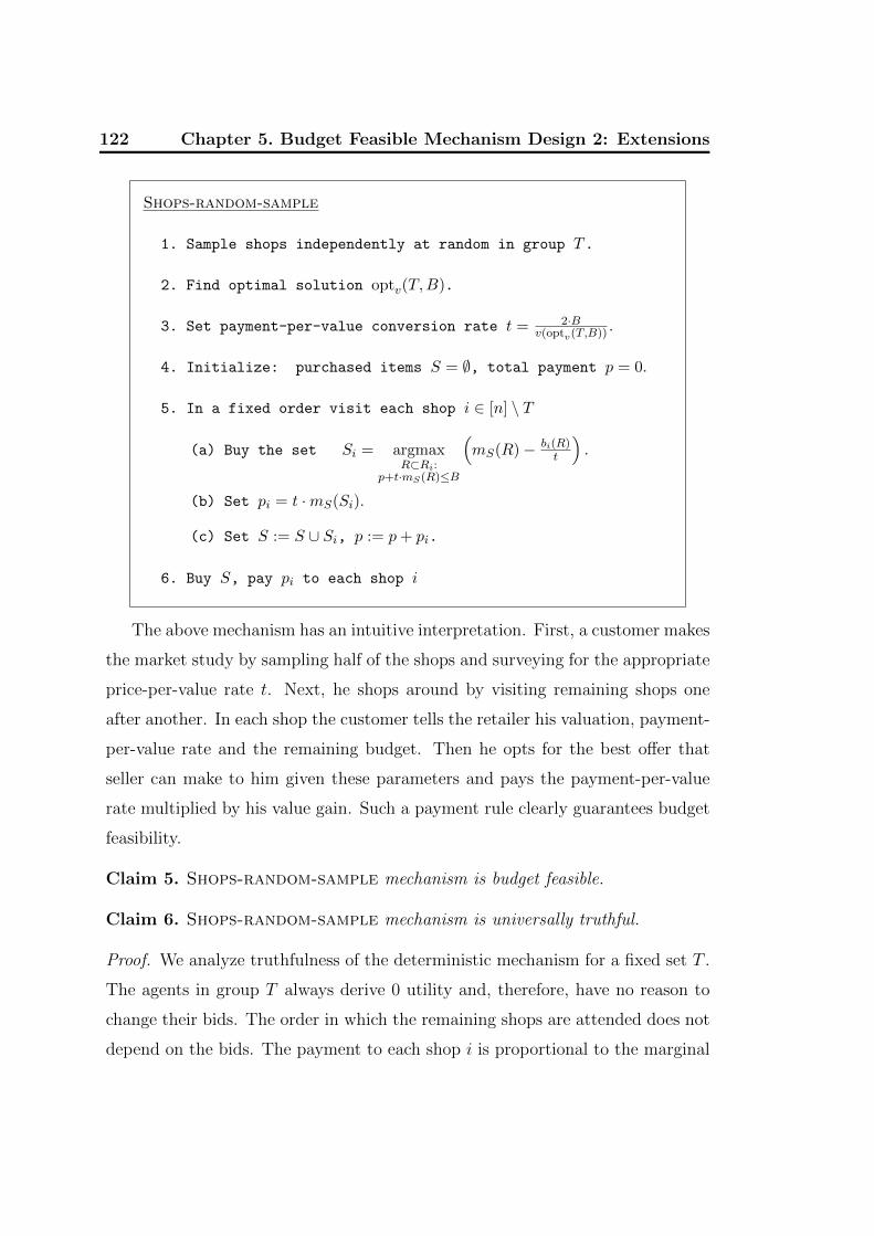
122 Chapter 5. Budget Feasible Mechanism Design 2: Extensions
Shops-random-sample
1. Sample shops independently at random in group T.
2. Find optimal solution optv(T,B).
3. Set payment-per-value conversion rate t = 2·Bv(optv(T,B)) .
4. Initialize: purchased items S = ∅, total payment p = 0.
5. In a fixed order visit each shop i ∈ [n] \ T
(a) Buy the set Si = argmaxR⊂Ri:
p+t·mS(R)≤B
(mS(R)− bi(R)
t
).
(b) Set pi = t ·mS(Si).
(c) Set S := S ∪ Si, p := p+ pi.
6. Buy S, pay pi to each shop i
The above mechanism has an intuitive interpretation. First, a customer makes
the market study by sampling half of the shops and surveying for the appropriate
price-per-value rate t. Next, he shops around by visiting remaining shops one
after another. In each shop the customer tells the retailer his valuation, payment-
per-value rate and the remaining budget. Then he opts for the best offer that
seller can make to him given these parameters and pays the payment-per-value
rate multiplied by his value gain. Such a payment rule clearly guarantees budget
feasibility.
Claim 5. Shops-random-sample mechanism is budget feasible.
Claim 6. Shops-random-sample mechanism is universally truthful.
Proof. We analyze truthfulness of the deterministic mechanism for a fixed set T .
The agents in group T always derive 0 utility and, therefore, have no reason to
change their bids. The order in which the remaining shops are attended does not
depend on the bids. The payment to each shop i is proportional to the marginal
5.2 Multi Item Sellers 123
value that auctioneer gains from items of i, i.e., pi = t · mS(Si). Further, the
utility of agent i is
ui = pi −∑j∈Si
cj = t ·(mS(Si)−
c(Si)
t
).
Given that t is a constant, in Step 5(a) the auctioneer picks the set R = Si,
which maximizes the above utility ui given bid bi and budget constraint p+pi ≤ B.
Si = argmaxR⊂Ri:
p+t·mS(R)≤B
(mS(R)− bi(R)
t
).
Thereby, the agent i maximizes his utility when reporting truthfully.
Unfortunately, Shops-random-sample mechanism may not always appro-
ximate benchmark opt∗ well. A bad instance contains only two shops, where the
first shop sells a single item X and the second shop sells single item Y , each item
at arbitrary price smaller than budget B; the auctioneer’s valuation v is additive
function with v(X) = 1, v(Y ) = 100. The benchmark has value opt∗ = 1. The
only possibility for the auctioneer to buy anything and derive non zero value is
when the first shop gets sampled in T and the second shop does not. In this case
t = 2·B1
and then the auctioneer estimates item Y too high, so that he simply
cannot afford to pay t ·m∅(Y ) = 200 · B for the item. Thus the expected value
of the mechanism is 0.
The problem we encounter here is due to the integrality issues in knapsack
packing. Indeed, if we would allow to buy a fraction of an item then mechanism
would have bought 1200
fraction of Y in the latter case and would obtain the value
of 12
and thus total expected value of 18. To circumvent this integral issues we
employ a complementary mechanism, which is given below.

124 Chapter 5. Budget Feasible Mechanism Design 2: Extensions
Exclusive-supplier
1. Sample shops independently at random in group T.
2. Find optimal solution optv(T,B).
3. Set value threshold tv = v(optv(T,B))4 .
4. In a fixed order visit each shop i ∈ [n] \ T
(a) Set S = argminR⊂Ri:v(R)≥tv
bi(R).
(b) If S 6= ∅ and bi(S) ≤ B Then buy S; pay pi = B; halt.
5. Buy ∅, pay 0.
As before the above mechanism has an intuitive interpretation. At this time
our customer does market study again by sampling half of the shops. Then he
makes a survey and decides what should be his targeted value tv. Further, the
customer consequently visits the rest of the shops aiming for an exclusive supplier.
In other words, conditioned on the fact that a shop can supply his demanded value
tv, he takes any offer that shop can make and spends all his budget in that shop.
Each run of the mechanism the payment is either 0 or B, which ensures budget
feasibility.
Claim 7. Exclusive-supplier is budget feasible mechanism.
Claim 8. Exclusive-supplier is universally truthful mechanism.
Proof. The proof is similar to the proof of Claim 6. This time the auctioneer
sets the rule that the value of any purchased set S should meet the threshold tv.
Then he agrees with any offer of the shop that meets the condition v(S) ≥ tv
and pays all his budget. The potential utility of a shop i in case of such deal is
ui = B − ci(S). Clearly, this utility will be maximized if agent i bids his true
costs bi(j) = cj on each j ∈ Ri.

5.2 Multi Item Sellers 125
Finally our main universally truthful and budget feasible mechanism, that
runs uniformly at random one of Exclusive-supplier and Shops-random-
sample mechanism, has a constant approximation ratio w.r.t. the benchmark
opt∗.
Shops-mechanism-main
With probability 0.5 run Exclusive-supplier.
With probability 0.5 run Shops-random-sample.
Theorem 22. Shops-mechanism-main in universally truthful budget feasible
mechanism that in expectation gives a constant approximation to benchmark opt∗
for any submodular valuation v(·).
Proof. Budget feasibility and universal truthfulness hold due to the Claims 5, 6,
7, 8. We next sketch the idea of constant approximation guarantee. The full
argument is given in the next subsection.
Approximation analysis (idea). For each subset A ⊂ [n] of shops and cost vector
c we define a function f(A) as the maximum value one can achieve on the item
set ∪i∈ARi under the budget constraint. It turns out that f(·) is subadditive
function.
Using subadditivity of f(·) we show that f([n] \ T ) ≥ f(T ) ≥ opt∗ hap-
pens with some constant probability for selecting T . For these situations using
the properties of submodular function such as in Lemma 8, we show that ei-
ther Shops-random-sample or Exclusive-supplier mechanism must have
a value of at least f(T )4
. Thus we get a lower bound constant fraction of opt∗ on
the expected value of Shops-mechanism-main.
5.2.2 Approximation Analysis.
Here we describe in full details the proof of a constant approximation guarantee
on the performance of Shops-mechanism-main. We assume that all shops bid

126 Chapter 5. Budget Feasible Mechanism Design 2: Extensions
truthfully, i.e., bi(j) = cj.
Similarly to the previous chapter we first analyze how well the sampling part
approximates an optimal solution. We want first to warn reader that in the
multi-item case sampling agents is different from sampling items. Now every
agent represents a cluster of items that altogether are sampled or not in the set
T .
For each subset A ⊂ [n] of shops we define a function f(A) as a maximal
value one can get on the items ∪i∈ARi under the budget constraint. We note that
f(T ) = optv(T,B) for any T ⊂ [n]. We show below that f(·) is a subadditive
function provided that v(·) is subadditive valuation. We further show that f(·)is XOS function provided that v(·) is XOS.
Interestingly, f(·) is not necessarily submodular function even if v(·) is ad-
ditive. Here is an example with 3 shops, 4 items and additive valuation v(·):v(1) = 1, v(2) = 2, v(3) = 3, v(4) = 5; c(1) = 1, c(2) = 2, c(3) = 3, c(4) = 4;
seller’s budget is 5; first shop offers only item 1, second shop sells items 2 and
3, third shop offers item 4. Then f(2) = 5, f(23) = 5, f(123) = 6 and,
therefore, f(·) is not submodular.
Lemma 17. If v(·) is subadditive, then f(·) is subadditive. If v(·) is XOS, then
f(·) is XOS.
Proof. To verify the subadditivity we need to show f(X ∪ Y ) ≤ f(X) + f(Y ).
Let us assume that in an optimal budget feasible solution for f(X ∪ Y ) we buy
items SX spending BX from the agents in X and buy SY spending BY from the
agents in Y . Then f(X) ≥ v(SX), since we can afford to buy SX with budget
B. Similarly, f(Y ) ≥ v(SY ). Therefore, f(X) + f(Y ) ≥ v(SX) + v(SY ) ≥v(SX ∪ SY ) = f(X ∪ Y ).
In order to show that f(·) is XOS we may specify for each agent i ∈ [n] a part
of the budget we can spend on the items from Ri. Then f can be described as the
maximum taken over all possible additive functions fj in the representation of

5.2 Multi Item Sellers 127
v = maxNj=1 fj(·) with any possible set of budget constraints Bi on every bundle
Ri (Bi ≥ 0,∑|A|
i=1Bi = B). Clearly, each such function
fB1,...,Bnj (A) =
∑i∈A
maxYi⊂Ri:c(Yi)≤Bi
fj(Yi)
is additive as a function of A ⊂ [n] and
f(A) = maxj,B1,...,Bn
B1+···+Bn=B
fB1,...,Bnj (A).
We notice that in such description there are infinitely many (continuum)
of functions fB1,...,Bnj (·) and we are allowed to use only finitely many of them.
However, for each Bi there are only finitely many different quantities that make
any difference for the value of maxYi⊂Ri:c(Yi)≤Bi
fj(Yi). Thus we need to use only finitely
many sets of different Bi and get the representation of f as the maximum over
finitely many additive functions.
Our next lemma is reminiscent of Lemma 11.
Lemma 18. PrT[f([n] \ T ) ≥ f(T ) ≥ 1
6· opt∗
]≥ 1
4.
Proof. Recall that opt∗ = mini∗∈[n] f([n] \ i∗). First, we argue that there is a
partition of [n] into two disjoint sets S1 and S2, such that f(S1), f(S2) ≥ 13
opt∗.
We can start with S1 = [n], S2 = ∅ and move agents one by one from S1 to S2.
Unavoidably, there will be a moment when f(S2) is still less than 13
opt∗, but right
after we move an agent i from S1 to S2 we get f(S2∪i) ≥ 13
opt∗ . We notice that
at the same time f(S1) > 23
opt∗, since f is subadditive. If f(S1 \ i) ≥ 13
opt∗,
then we have found the required partition S1 \ i and S2 ∪ i. On the other
hand, if f(S1 \ i) < 13
opt∗, then f(i) ≥ f(S1)− f(S1 \ i) > 13
opt∗ . In such
a case we can simply take S1 = i and S2 = [n] \ i. Note that f(S1) ≥ 13
opt∗
and f(S2) = f([n] \ i) ≥ opt∗ by definition of opt∗.
Thus, we have a partition of [n] into S1 and S2 with f(S1) ≥ 13
opt∗ and
f(S2) ≥ 13
opt∗. Let us denote [n] \ T by T . Notice that when agents from S1 are
128 Chapter 5. Budget Feasible Mechanism Design 2: Extensions
sampled in T , either f(S1∩T ) ≥ 12f(S1) ≥ 1
6opt∗, or f(S1∩T ) ≥ 1
2f(S1) ≥ 1
6opt∗.
Moreover, each of these events happens with probability at least 0.5. We have
similar bounds for agents in S2, which are drawn in T independently from S1.
Hence, with probability at least 0.5 we have f(T ) ≥ 16
opt∗ and f(T ) ≥ 16
opt∗
simultaneously.
Therefore, PrT[min(f([n] \ T ), f(T )) ≥ 1
6· opt∗
]≥ 1
2. Due to the symmetry
between T and [n] \ T we get that f([n] \ T ) ≥ f(T ) with probability 0.5 in the
previous inequality. Therefore, PrT[f([n] \ T ) > f(T ) ≥ 1
6· opt∗
]≥ 1
4.
Now we are ready to estimate the expected value of Shops-mechanism-
main. Let us fix a sample set T with f(T ) ≤ f([n] \ T ) same for both Shops-
random-sample and Exclusive-supplier mechanisms. Let S be the output
set of items of Shops-random-sample mechanism and U be the optimal set of
items in [n] \ T under the budget constraint, i.e., v(U) = f([n] \ T ) ≥ f(T ) and
c(U) ≤ B; payment-per-value conversion rate t is 2Bf(T )
.
The total payment of Shops-random-sample mechanism is t · v(S), which
is below the budget B. Therefore, 2B·v(S)f(T )
≤ B and v(S) ≤ 0.5 · f(T ). We apply
Lemma 8 from the previous chapter to the sets U ∪S and S. It tells us that there
is item j0 ∈ U \ S, s.t.
mS(j0)
c(j0)≥ v(U ∪ S)− v(S)
c(U ∪ S)− c(S).
We observe that v(U∪S)−v(S)c(U∪S)−c(S)
≥ f(T )−0.5·f(T )c(U\S)
, since v(U ∪ S) ≥ v(U) ≥ f([n] \T ) ≥ f(T ) and v(S) ≤ 0.5f(T ). Further, v(U∪S)−v(S)
c(U∪S)−c(S)≥ 0.5·f(T )
B, because
c(U \ S) ≤ c(U) ≤ B. Since 0.5·f(T )B
= 1t, we have the following observation
Claim 9. There is an item j0 ∈ U \ S s.t. mS(j0) ≥ t · c(j0).
Let us examine the question why the item j0 did not appear in the final set
S. At certain point the shop i with j0 ∈ Ri was considered in Step 5 of Shops-
random-sample mechanism and item j0 was not included in Si. We recall that

5.2 Multi Item Sellers 129
Si = argmaxR⊂Ri:
p+t·mS(i)(R)≤B
(mS(i)(R)− c(R)
t
),
where S(i) is the current set of winners S selected right before the visit
to shop i in the Shops-random-sample mechanism. Note that at this mo-
ment mS(i)∪Si(j0) could be only larger then the final quantity mS(j0) due to
submodularity of v(·). Hence, if in the mechanism we added j0 to the set Si,
then the value of mS(i)(Si) − c(Si)t
would only increase. Therefore, the only
reason why we did not include j0 in Si is because of the budget constraint.
That is, the payment of the mechanism would be larger than B. Equivalently,
v(S ∪j0) = v(S) +mS(j0) ≥ f(T )2
, because the total payment is proportional to
the total value with the coefficient 2Bf(T )
. In particular, we can make the following
observation.
Claim 10. If v(S) ≤ f(T )4
, then mS(j0) ≥ f(T )4.
First we notice that if v(S) > f(T )4
then Shops-random-sample mechanism
provides a constant approximation to f(T ).
Second, if v(S) ≤ f(T )4
, then mS(j0) ≥ f(T )4. We notice that then v(j0) ≥
mS(j0) ≥ tv, where tv = f(T )4
in Exclusive-supplier mechanism. Therefore,
Exclusive-supplier mechanism must output a nonempty set with total value
of at least tv = f(T )4.
Combining the above two lower bounds, we obtain that the expected value of
Shops-mechanism-main in case f([n] \ T ) ≥ f(T ) must be at least 0.5 · f(T )4
.
Using this lower bound and Lemma 18 we obtain that expected value of Shops-
mechanism-main must be at least
PrT
[f([n] \ T ) ≥ f(T ) ≥ 1
6· opt∗
]·(
0.5 · f(T )
4
)≥ opt∗
192,
which is a constant approximation to the benchmark opt∗.

130 Chapter 5. Budget Feasible Mechanism Design 2: Extensions
5.2.3 Computational Issues
The main mechanism as it is described does not work in polynomial time, however
it may be implemented “almost” efficiently. Remarks on the efficient implemen-
tation of mechanisms Shops-random-sample and Exclusive-supplier are in
order below.
1. Instead of using an optimal solution optv(T,B), which is NP-hard to
find for a general submodular function v, we may efficiently find a solution
that approximates the optimum by a constant factor. Indeed, an approximate
solution to the budgeted submodular maximization problem can be found in
polynomially many value queries [51]. We notice that substituting optimum with
an approximate solution in the sampling part does not affect truthfulness, but
may decrease the approximation guarantees by a constant factor.
2. Step 5 of Shops-random-sample and Step 4 of Exclusive-supplier
mechanisms in general are hard to implement, even if we are granted access
to a more powerful demand oracle for the valuation v(·). However, if every
shop is selling only a few items (number is bounded by a constant), then we
can implement Shops-mechanism-main in polynomial time. We note that
substituting Si = argmax(·) or S = argmin(·) in each Step 5 or Step 4 with
an approximate solution would change the value of the final mechanism only by
a constant factor. Unfortunately, such a substitution is not incentive compatible.
3. In general case our main mechanism, formally speaking, cannot be im-
plemented in polynomial time, but speaking practically, it actually may be ef-
ficiently implemented. Let us consider, for instance, a problematic Step 5 of
Shops-random-sample mechanism. We already have convinced ourselves that
the selection rule in Step 5(a) and the payment rule in Step 5(b) are aligned with
the utility maximization objective of the seller i. Thereby, the objectives of the
shop and the auctioneer at this point do coincide and there should not be a prob-
lem for both parties to find an agreement. In particular, using only value queries,
the auctioneer may efficiently find a good candidate set Si and suggest it to shop

5.2 Multi Item Sellers 131
i. The shop in its turn, having the access to valuation function v(·) and observing
the remaining auctioneer’s budget B − p, may try to find a better solution S ′i.
Remarkably, the shop, in order to increase its utility, is only interested to propose
a better set S ′i than that of Si. Auctioneer will agree on every such S ′i as long as
it meets all of his easy-to-verify criteria. In this “dialog” between the auctioneer
and the seller i, the shop i does not have any incentive to misreport its costs.
Indeed, the computational task of figuring out a beneficial bid bi different from
shop’s true costs may be only harder than the task of proposing a better set S ′i
to the auctioneer. A similar “efficient dialog” between auctioneer and a shop can
be implemented in Exclusive-supplier mechanism as well. To sum up, our
auctioneer gets in polynomial time a solution that is a constant approximation
to the benchmark, while all the shops report truthfully.
Remark 5. In the field of algorithmic mechanism design it is commonly required
that a mechanism, upon receiving the bids from agents, should decide in polyno-
mially many steps on the set of winners and payments, while ensuring incentive
compatibility of these decision rules. The latter observation raises a critical point
against this classic definition of efficient implementation of a mechanism. It also
suggest an extra round of communication between agents and the mechanism de-
signer.
We propose below a relaxed definition, where an extra round of communication
is allowed between auctioneer and agents.
Definition 8. First, mechanism M receives the bid vector b from each of n
agents, which may be different from the true cost vector c. Then M applies a
communication protocol exchanging messages with the agents, each time sending
to and receiving reply from an agent i ∈ [n]. The mechanism keeps the record ri
on all the replies from every agent i. The total length of the replies r = (ri)i∈[n]
and the messages sent in the protocol must be bounded by a polynomial in n.
Moreover, we assume that M can only perform computations in polynomial in

132 Chapter 5. Budget Feasible Mechanism Design 2: Extensions
n time. Therefore, each subsequent massage it sends to an agent must be easy
to compute for a given bid vector and previous agent’s replies. Based on the bid
vector b and replies r = (ri)i∈[n], the final decision on the winning set S(b, r)
and payments p(b, r) is made. We call the mechanism M truthful, if for each
agent i and fixed bids b−i and replies r−i of other agents there exists efficiently
computable function fi, s.t.
∀bi′, r′i ui (bi′,b−i, r
′i, r−i) ≤ ui(ci,b−i, fi(bi
′, r′i), r−i).
In other words, mechanism is truthful if and only if any misreported bid of an
agent can be effectively turned into at least as good true bid with an appropriate
reply message.
The performance of such a mechanism should be measured in the case of worst
possible replies provided by the agents.
Chapter 6Conclusions and Open Problems
In this work we examined two important classes of optimization problems in
algorithmic mechanism design. For the first class, we proposed a unified scheme
for designing frugal incentive compatible mechanisms. We showed that several
existing mechanisms fall under our scheme, and described its applications to
k-path systems and vertex cover systems. We demonstrated that our scheme
produces mechanisms with good ν-frugality ratios for k-path systems and a
large subclass of vertex cover systems; for k-path systems, we showed that
our mechanism has the optimal µ-frugality ratio and can be implemented in
polynomial time.
For the second class, we proposed a number of constant approximation in-
centive compatible mechanisms for most of the valuation classes in the hierarchy
of complement free functions. We gave the positive answer to the “fundamental
question” raised in [30] by presenting a constant approximation mechanism in
the Bayesian framework and showing via Yao’s min-max principle the existence
of constant approximation mechanism in the prior-free framework. We presented
two prior-free truthful mechanisms of integrality-gap and sub-logarithmic worst-
case approximations to the optimum, as well as a Bayesian constant approxima-
tion incentive compatible mechanism, and provided an efficient implementation
of our sub-logarithmic mechanism. We proposed a new extension of the original
133

134 Chapter 6. Conclusions and Open Problems
model to the scenario with multi-item sellers and gave a constant approximation
incentive compatible mechanism for an arbitrary submodular valuation.
Certainly, much work is left to be done in the area of frugal mechanism design.
Beyond k-paths and vertex cover auctions, there are many other set systems in
which frugal mechanism design can be applied, e.g., Matching, Independent Set
etc. While there exist preliminary studies on some of these settings, their optimal
designs still remain a mystery. Thereby, the important question “what are the
(nearly) optimal designs of frugal mechanisms in different procurement auctions?”
remains widely open.
In the budget feasible model many open questions remain as well. In par-
ticular, for the model with multi-item sellers it is not known whether constant
approximation mechanisms exist for XOS and subadditive valuaitons. In the
unit-item seller model, for those mechanisms with exponential runtime, it is nat-
ural to ask if there are truthful designs with the same approximations that can be
implemented in polynomial time. Further, all of our mechanisms are randomized;
it is intriguing to consider the approximability of deterministic mechanisms. We
are also looking for other, not complement free, classes of valuations that admit
budget feasible mechanisms with good approximation ratios.
List of Publications
1. Computing approximate pure Nash equilibria in congestion games, I. Caragiannis,
A. Fanelli, N. Gravin, A. Skopalik, SIGecom Exchanges 2012, p. 26-29.
2. Approximate Pure Nash Equilibria in Weighted Congestion Games:Existence,
Efficient Computation, and Structure, I. Caragiannis, A. Fanelli, N. Gravin, A.
Skopalik, EC 2012, p. 284-301.
3. Budget Feasible Mechanism Design: From Prior-Free to Bayesian X. Bei, N.
Chen, N. Gravin, P. Lu, STOC 2012, p. 449-458.
4. Efficient computation of approximate pure Nash equilibria in congestion games,
I. Caragiannis, A. Fanelli, N. Gravin, A. Skopalik, FOCS 2011, p. 532-541.
5. Dynamics of Profit-Sharing Games, J. Augustine, N. Chen, E. Elkind, A. Fanelli,
N. Gravin, D. Shiryaev, IJCAI 2011, p. 37-42.
6. On the Approximability of Budget Feasible Mechanisms, N. Chen, N. Gravin, P.
Lu, SODA 2011, p. 685-699.
7. Note on Shortest k-Paths Problem, N. Chen, N. Gravin, Journal of Graph Theory.
V. 67(1), 2011 p. 34-37.
8. Frugal Mechanism Design via Spectral Techniques, N. Chen, E. Elkind, N. Gravin,
F. Petrov, FOCS 2010, p. 755-764.
9. Refining the Cost of Cheap Labor in Set System Auctions, N. Chen, E. Elkind
and N. Gravin, WINE 2009, p. 447-454.
135


Bibliography
[1] G. Aggarwal and J. D. Hartline. Knapsack auctions. In SODA, pages 1083–1092,
2006.
[2] A. Archer and E. Tardos. Truthful mechanisms for one-parameter agents. In
FOCS, pages 482–491, 2001.
[3] A. Archer and E. Tardos. Frugal path mechanisms. In SODA, pages 991–999,
2002.
[4] M. Babaioff, M. Dinitz, A. Gupta, N. Immorlica, and K. Talwar. Secretary
problems: weights and discounts. In SODA, pages 1245–1254, 2009.
[5] M. Babaioff, N. Immorlica, and R. Kleinberg. Matroids, secretary problems, and
online mechanisms. In SODA, pages 434–443, 2007.
[6] A. Badanidiyuru, S. Dobzinski, and S. Oren. Optimization with demand oracles.
In ACM Conference on Electronic Commerce, pages 110–127, 2012.
[7] A. Badanidiyuru, R. Kleinberg, and Y. Singer. Learning on a budget: posted price
mechanisms for online procurement. In ACM Conference on Electronic Commerce,
pages 128–145, 2012.
[8] R. Bar-Yehuda and S. Even. A local-ratio theorem for approximating the weighted
vertex cover problem. North-Holland Mathematics Studies, 109(C):27–45, 1985.
[9] X. Bei, N. Chen, N. Gravin, and P. Lu. Budget feasible mechanism design: from
prior-free to bayesian. In STOC, pages 449–458, 2012.
137

138 Bibliography
[10] X. Bei and Z. Huang. Bayesian incentive compatibility via fractional assignments.
In SODA, pages 720–733, 2011.
[11] S. Bhattacharya, G. Goel, S. Gollapudi, and K. Munagala. Budget constrained
auctions with heterogeneous items. In STOC, pages 379–388, 2010.
[12] K. Bhawalkar and T. Roughgarden. Welfare guarantees for combinatorial auctions
with item bidding. In SODA, pages 700–709, 2011.
[13] O. Bondareva. Some applications of linear programming to cooperative games.
Problemy Kibernetiki, 10:119–139, 1963.
[14] G. Calinescu. Bounding the payment of approximate truthful mechanisms. In
ISAAC, pages 221–233, 2004.
[15] S. Chawla, J. D. Hartline, D. L. Malec, and B. Sivan. Multi-parameter mechanism
design and sequential posted pricing. In STOC, pages 311–320, 2010.
[16] S. Chawla, D. L. Malec, and A. Malekian. Bayesian mechanism design for budget-
constrained agents. In ACM Conference on Electronic Commerce, pages 253–262,
2011.
[17] S. Chawla, D. L. Malec, and B. Sivan. The power of randomness in bayesian
optimal mechanism design. In ACM Conference on Electronic Commerce, pages
149–158, 2010.
[18] N. Chen, E. Elkind, N. Gravin, and F. Petrov. Frugal mechanism design via
spectral techniques. In FOCS, pages 755–764, 2010.
[19] N. Chen and N. Gravin. A note on k-shortest paths problem. Journal of Graph
Theory, 67(1):34–37, 2011.
[20] N. Chen, N. Gravin, and P. Lu. Mechanism design without money via stable
matching. CoRR, abs/1104.2872, 2011.
[21] N. Chen, N. Gravin, and P. Lu. On the approximability of budget feasible
mechanisms. In SODA, pages 685–699, 2011.
[22] N. Chen and A. R. Karlin. Cheap labor can be expensive. In SODA, pages 707–715,
2007.
[23] E. H. Clarke. Multipart pricing of public goods. Public Choice, 11:17–33, 1971.

Bibliography 139
[24] A. Czumaj and A. Ronen. On the expected payment of mechanisms for task
allocation. In PODC, pages 98–106, 2004.
[25] K. David. personal communication.
[26] N. R. Devanur, J. D. Hartline, A. R. Karlin, and C. T. Nguyen. Prior-independent
multi-parameter mechanism design. In WINE, pages 122–133, 2011.
[27] P. Dhangwatnotai, T. Roughgarden, and Q. Yan. Revenue maximization with a
single sample. In ACM Conference on Electronic Commerce, pages 129–138, 2010.
[28] S. Dobzinski. Two randomized mechanisms for combinatorial auctions. In
APPROX-RANDOM, pages 89–103, 2007.
[29] S. Dobzinski, R. Lavi, and N. Nisan. Multi-unit auctions with budget limits. In
FOCS, pages 260–269, 2008.
[30] S. Dobzinski, C. H. Papadimitriou, and Y. Singer. Mechanisms for complement-
free procurement. In ACM Conference on Electronic Commerce, pages 273–282,
2011.
[31] E. Elkind. True costs of cheap labor are hard to measure: edge deletion and vcg
payments in graphs. In ACM Conference on Electronic Commerce, pages 108–116,
2005.
[32] E. Elkind, L. A. Goldberg, and P. W. Goldberg. Frugality ratios and improved
truthful mechanisms for vertex cover. In ACM Conference on Electronic Com-
merce, pages 336–345, 2007.
[33] E. Elkind, A. Sahai, and K. Steiglitz. Frugality in path auctions. In SODA, pages
701–709, 2004.
[34] U. Feige. On maximizing welfare when utility functions are subadditive. SIAM J.
Comput., 39(1):122–142, 2009.
[35] U. Feige, V. S. Mirrokni, and J. Vondrak. Maximizing non-monotone submodular
functions. In FOCS, pages 461–471, 2007.
[36] J. Feigenbaum, C. H. Papadimitriou, R. Sami, and S. Shenker. A bgp-based
mechanism for lowest-cost routing. In PODC, pages 173–182, 2002.

140 Bibliography
[37] A. Ghosh and A. Roth. Selling privacy at auction. In ACM Conference on
Electronic Commerce, pages 199–208, 2011.
[38] C. Godsil and G. Royle. Algebraic graph theory, volume 207 of Graduate Texts in
Mathematics. Springer-Verlag, New York, 2001.
[39] A. Goldberg, J. Hartline, A. Karlin, M. Saks, and A. Wright. Competitive auctions.
Games and Economic Behavior, 55(2):242–269, 2006.
[40] A. V. Goldberg, J. D. Hartline, and A. Wright. Competitive auctions and digital
goods. In SODA, pages 735–744, 2001.
[41] A. V. Goldberg and R. E. Tarjan. Finding minimum-cost circulations by canceling
negative cycles. J. ACM, 36(4):873–886, 1989.
[42] T. Groves. incentives in teams. Econometrica, 41(4):617–631, 1973.
[43] G. H. Hardy, J. E. Littlewood, and G. Polya. Inequalities. Cambridge university
press, 1952.
[44] J. D. Hartline, R. Kleinberg, and A. Malekian. Bayesian incentive compatibility
via matchings. In SODA, pages 734–747, 2011.
[45] J. D. Hartline and B. Lucier. Bayesian algorithmic mechanism design. In STOC,
pages 301–310, 2010.
[46] J. D. Hartline and T. Roughgarden. Optimal mechanism design and money
burning. In STOC, pages 75–84, 2008.
[47] N. Immorlica, D. R. Karger, E. Nikolova, and R. Sami. First-price path auctions.
In ACM Conference on Electronic Commerce, pages 203–212, 2005.
[48] A. Iwasaki, D. Kempe, Y. Saito, M. Salek, and M. Yokoo. False-name-proof
mechanisms for hiring a team. In WINE, pages 245–256, 2007.
[49] A. R. Karlin, D. Kempe, and T. Tamir. Beyond vcg: Frugality of truthful
mechanisms. In FOCS, pages 615–626, 2005.
[50] D. Kempe, M. Salek, and C. Moore. Frugal and truthful auctions for vertex covers,
flows and cuts. In FOCS, pages 745–754, 2010.

Bibliography 141
[51] A. Krause and C. Guestrin. A note on the budgeted maximization of submodular
functions. Technical Report CMU-CALD-05-103, School of Computer Science
Carnegie Mellon University, 2005.
[52] V. Krishna. Auction Theory. Academic Press, San Diego, 2003.
[53] J. Lee, V. S. Mirrokni, V. Nagarajan, and M. Sviridenko. Non-monotone sub-
modular maximization under matroid and knapsack constraints. In STOC, pages
323–332, 2009.
[54] B. Lehmann, D. J. Lehmann, and N. Nisan. Combinatorial auctions with decreas-
ing marginal utilities. In ACM Conference on Electronic Commerce, pages 18–28,
2001.
[55] K. Menger. Zur allgemeinen kurventheorie. Fundamenta Mathematicae, 10:96–115,
1927.
[56] P. Milgrom. Putting auction theory to work: The simultaneous ascending auction.
Journal of Political Economy, 108(2):245–272, 2000.
[57] R. B. Myerson. Optimal auction design. Math. Oper. Res., 6(1):58–73, 1981.
[58] G. Nemhauser, L. Wolsey, and M. Fisher. An analysis of approximations for
maximizing submodular set functions-i. Mathematical Programming, 14(1):265–
294, 1978.
[59] N. Nisan and A. Ronen. Algorithmic mechanism design (extended abstract). In
STOC, pages 129–140, 1999.
[60] N. Nisan, T. Roughgarden, E. Tardos, and V. V. Vazirani. Algorithmic Game
Theory. Cambridge University Press, New York, NY, USA, 2007.
[61] A. D. Procaccia and M. Tennenholtz. Approximate mechanism design without
money. In ACM Conference on Electronic Commerce, pages 177–186, 2009.
[62] L. S. Shapley. On balanced sets and cores. Naval Research Logistics Quarterly,
14(4):453–460, 1967.
[63] Y. Singer. Budget feasible mechanisms. In FOCS, pages 765–774, 2010.
[64] Y. Singer. Incentives, Computation, and Networks: Limitations and Possibilities
of Algorithmic Mechanism Design. PhD thesis, UC Berkeley, 2011.

142 Bibliography
[65] C. Stone. A Course in Probability and Statistics. Duxbury Press, 1995.
[66] M. Sviridenko. A note on maximizing a submodular set function subject to a
knapsack constraint. Oper. Res. Lett., 32(1):41–43, 2004.
[67] K. Talwar. The price of truth: Frugality in truthful mechanisms. In STACS, pages
608–619, 2003.
[68] W. Vickrey. Counterspeculation, auctions, and competitive sealed tenders. journal
of finance, 16(1):8–37, 1961.
[69] Q. Yan. On the price of truthfulness in path auctions. In WINE, pages 584–589,
2007.