Multi-Objective Optimisation Techniques in Reservoir Simulation

Mike Christie

Heriot-Watt University

Outline

• Introduction

• Stochastic Optimisation

• Model Calibration

• Forecasting

• Reservoir Optimisation

• Summary

Outline

• Introduction

• Stochastic Optimisation

• Model Calibration

• Forecasting

• Reservoir Optimisation

• Summary

Mathematics of Flow in Porous Media

• Conservation of Mass

• Conservation of Momentum

– replaced by Darcy’s law

• Conservation of Energy

– most processes isothermal

• Equation of State

kp

xv

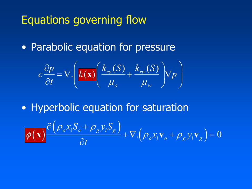
• Parabolic equation for pressure

• Hyperbolic equation for saturation

( ) ( ). ( ) ro rw

o w

k S k Spc k p

t

x

. 0o i o g i g

o i o g i g

x S y Sx y

t

x v v

Equations governing flow

Data Collection

?

?k

x

x

Model Calibration: Teal South

0

500

1000

1500

2000

2500

0 200 400 600 800 1000 1200 1400

time (days)

simulated

observed

0

200

400

600

800

1000

0 200 400 600 800 1000 1200 1400

time (days)

simulated

observed

2000

2200

2400

2600

2800

3000

3200

0 200 400 600 800 100012001400

time (days)

simulated

observed

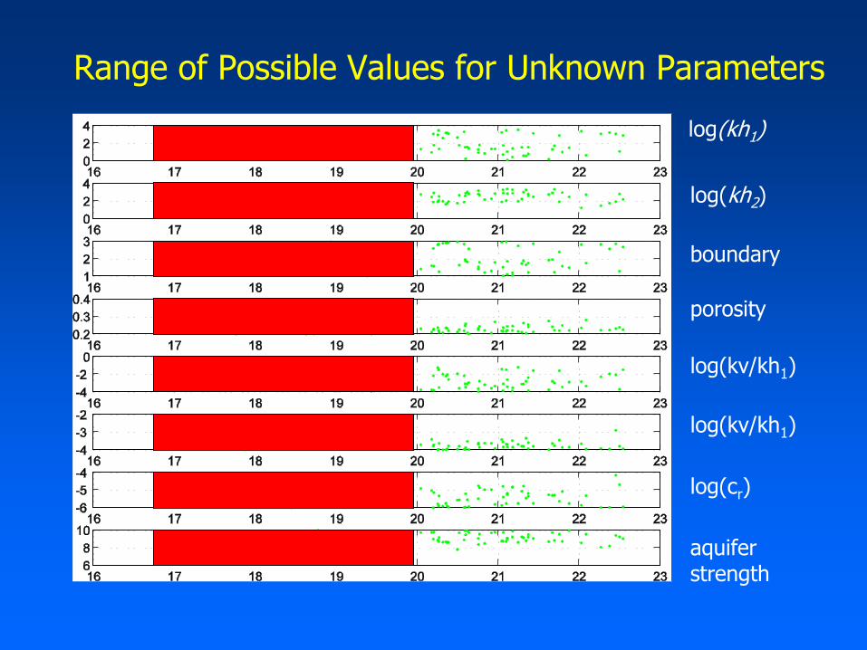
Range of Possible Values for Unknown Parameters

log(kh1)

log(kh2)

boundary

porosity

log(kv/kh1)

log(kv/kh1)

log(cr)

aquifer strength

Outline

• Introduction

• Stochastic Optimisation

• Model Calibration

• Forecasting

• Reservoir Optimisation

• Summary

Particle Swam Optimization (PSO)

• A swarm intellegence algorithm (Kennedy & Eberhart,1995).

• Particles are points in parameter space.

• Particles move based on their own experience and that of the swarm.

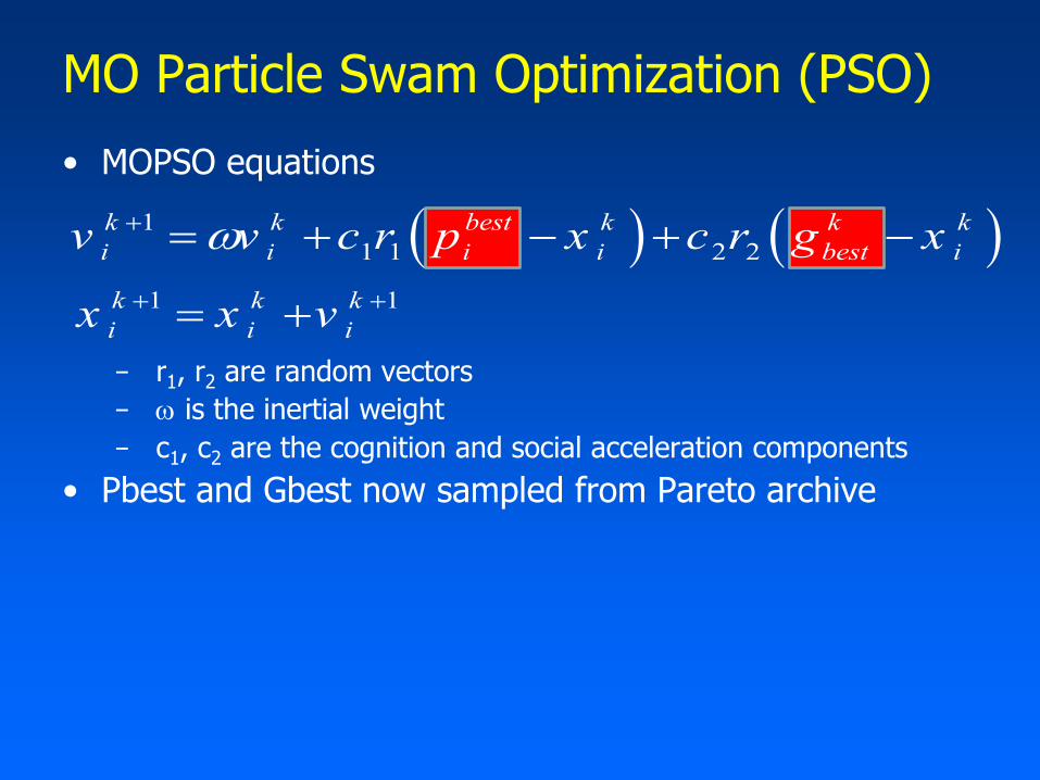
• PSO equations

− r1, r2 are random vectors

− w is the inertial weight

− c1, c2 are the cognition and social acceleration components

1

1 1 2 2

1 1

k k best k k k

i i i i best i

k k k

i i i

v v c r p x c r g x

x x v

w

Dominance and Pareto Optimality

Solution 𝐱𝟏 dominates solution 𝐱𝟐, if :

1. 𝐱𝟏 is no worse than 𝐱𝟐 in all objectives, and

2. 𝐱𝟏 is strictly better than 𝐱𝟐 in at least one objective

Ob

j 2

Obj 1

Pareto front

Image of Pareto optimal set in objective space

1

1 1 2 2

1 1

k k best k k k

i i i i best i

k k k

i i i

v v c r p x c r g x

x x v

w

• MOPSO equations

− r1, r2 are random vectors

− w is the inertial weight

− c1, c2 are the cognition and social acceleration components

• Pbest and Gbest now sampled from Pareto archive

MO Particle Swam Optimization (PSO)

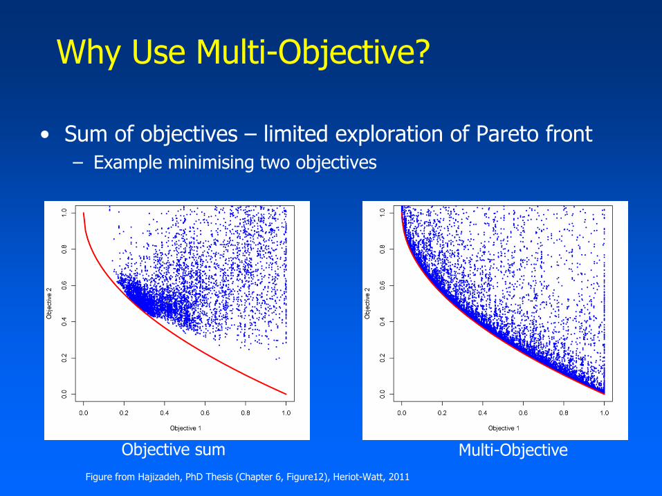
Why Use Multi-Objective?

• Sum of objectives – limited exploration of Pareto front

– Example minimising two objectives

Objective sum Multi-Objective

Figure from Hajizadeh, PhD Thesis (Chapter 6, Figure12), Heriot-Watt, 2011

Outline

• Introduction

• Stochastic Optimisation

• Model Calibration

• Forecasting

• Reservoir Optimisation

• Summary

Model Calibration

• Called ‘History Matching’ in oil business

• Synthetic example

– IC Fault Model

• Real example

– Zagadka Field

IC Fault Model

*

* Data from Z. Tavassoli, Jonathan N. Carter, and Peter R. King,

Imperial College, London

• Synthetic 2D Model

• 2 Wells: 1 Inj, 1 Prod

• 6 Layers

• 1,3,5 Poor Sand (blue)

• 2,4,6 Good Sand (red)

• 1 Fault

• 3 Uncertain Inputs: 1. khigh = [100,200] mD

2. klow = [0,50] mD

3. throw = [0,60] ft

IC Fault Model

p : oil/water rates

Truth Profile (Observed) Observed

khigh = 131.6 mD

klow = 1.3 mD

throw = 10.4 ft

Misfit Definition:

• Simulator controlled to match BHP at the wells

2

2

1

2

0.03

p t

sim obsM

n

obs

IC Fault Model Misfit Surface

high low

misfit

klow

khigh

throw

Database (DB) 159,661 uniformly generated models

truth

Convergence Speed – 20 Runs

MOPSO

SOPSO

Iteration 12

Iteration 28

Zagadka Field

• Waterflood/aquifer support

• 95 wells in 10 groups

• 15 years history

• Compartmentalized

Model 4 Convergence (PSO)

500

700

900

1100

1300

1500

1700

1900

0 50 100 150 200 250

Mis

fit

Iteration

Model 4 Field Level History Match

• Match with PSO (single objective)

• 250 simulations (overnight, 12 core workstation)

Field oil rate Field water rate

Match on Group Rates – Single Objective

Multi-Objective vs Single Objective

500

550

600

650

700

750

800

850

900

950

1000

0 50 100 150 200 250 300

Min

imum

Mis

fit

Iteration

PSO

MOPSO

Multi-Objective Trade Off

• MO balances changes to fit one quantity vs another

MO Not Always Faster than SO

• Study on EoN field

Histogram of 10 Final Misfits

Outline

• Introduction

• Stochastic Optimisation

• Model Calibration

• Forecasting

• Reservoir Optimisation

• Summary

Forecasting with MO

• Generic Bayesian integral

• MC approximation

• Resample to calculate P(mk)dVk

( ) ( )

eg mean oil rate ( ) ( )o

J g P d

Q P d

m m m

m m m

1 1

1 1N Nk k

k k k

k kk

g PJ g P dV

N h N

m m

m mm

Calculating Weights for Sample

• Gibbs sampler

– Assume misfit constant in Voronoi cell

Single & Multi Objective HM for PUNQ-S3

Based on real field

An industry standard benchmark

Multiple wells and production variables

Algorithm used: PSO

SO vs. MO – Forecasting

Time (days)

Time (days)

FO

PT (

sm3)

Time (days)

FO

PT (

sm3)

FW

PT (

sm3)

Time (days)

FW

PT (

sm3)

Outline

• Introduction

• Stochastic Optimisation

• Model Calibration

• Forecasting

• Reservoir Optimisation

• Summary

Field Development Optimisation

• Based on Scapa field

– Original HM done as part of MSc project

– HM to field rates (from DECC website)

– Wells are different from real field

• 4 injectors, 4 producers

Field Level History Match

• Match to first 10 years of history

– Remaining data used to check forecast

Optimisation

• Multi-Objective

– Maximise cumulative oil (FOPT)

– Minimise maximum water rate (FWPR)

• Optimisation variables

– Well locations (16 variables – i, j for each well)

– Injection well rates

Field Development Optimisation (Scapa)

Optimise Field Development Plan

Original MSc development plan (4 injectors, 4 producers)

10%

55%

77 models

Current Scapa production

Scapa: Optimise Mid-Life Infill Wells

Trade-off : 1.5 bbls oil in year 10 for 1 bbl oil in year 2

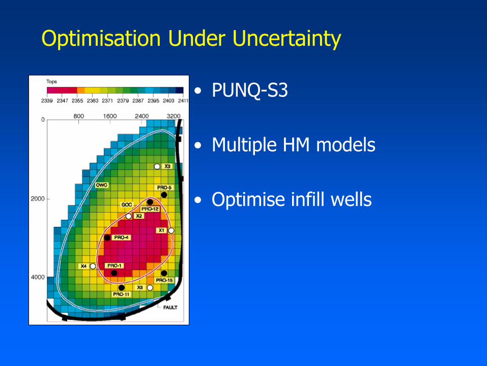
Optimisation Under Uncertainty

• PUNQ-S3

• Multiple HM models

• Optimise infill wells

Optimisation Under Uncertainty

Uncertainty in Cumulative Oil

Mean C

um

ula

tive O

il

Summary

• History Matching

– Multi-objective may increase convergence speed, but not always

• Forecasting

– Multi-objective provides greater coverage of pareto front; can lead to better forecasts

• Optimisation

– Explore the full range of trade-offs

– Can include uncertainty

Acknowledgements

• EoN for funding the SO vs MO comparison

• BG, EoN, JOGMEC, RFD for funding the uncertainty group at HW

• Schlumberger for licences of ECLIPSE

• RFD for licences of tNavigator