multi-curve modelling using trees - springer · pdf filemulti-curve modelling using trees ......

Multi-curve Modelling Using Trees

John Hull and Alan White

Abstract Since2008 thevaluationof derivatives has evolved so thatOISdiscountingrather than LIBOR discounting is used. Payoffs from interest rate derivatives usuallydepend on LIBOR. This means that the valuation of interest rate derivatives dependson the evolution of two different term structures. The spread betweenOIS andLIBORrates is often assumed to be constant or deterministic. This paper explores how thisassumption can be relaxed. It shows how well-established methods used to representone-factor interest rate models in the form of a binomial or trinomial tree can beextended so that the OIS rate and a LIBOR rate are jointly modelled in a three-dimensional tree. The procedures are illustrated with the valuation of spread optionsand Bermudan swap options. The tree is constructed so that LIBOR swap rates arematched.

Keywords OIS · LIBOR · Interest rate trees · Multi-curve modelling

1 Introduction

Before the 2008 credit crisis, the spread between a LIBOR rate and the correspondingOIS (overnight indexed swap) rate was typically around 10 basis points. During thecrisis this spread rose dramatically. This led practitioners to review their derivativesvaluation procedures. A result of this review was a switch from LIBOR discountingto OIS discounting.

Finance theory argues that derivatives can be correctly valued by estimating ex-pected cash flows in a risk-neutral world and discounting them at the risk-free rate.The OIS rate is a better proxy for the risk-free rate than LIBOR.1 Another argument

1See for example Hull and White [15].

J. Hull (B) · A. WhiteJoseph L. Rotman School of Management, University of Toronto, Toronto, ON, Canadae-mail: [email protected]

A. Whitee-mail: [email protected]

© The Author(s) 2016K. Glau et al. (eds.), Innovations in Derivatives Markets, Springer Proceedingsin Mathematics & Statistics 165, DOI 10.1007/978-3-319-33446-2_9

171

172 J. Hull and A. White

(appealing to many practitioners) in favor of using the OIS rate for discounting isthat the interest paid on cash collateral is usually the overnight interbank rate andOIS rates are longer term rates derived from these overnight rates. The use of OISrates therefore reflects funding costs.

Many interest rate derivatives provide payoffs dependent on LIBOR. When LI-BOR discounting was used, only one rate needed to be modelled to value thesederivatives. Now that OIS discounting is used, more than one rate has to be consid-ered. The spread between OIS and LIBOR rates is often assumed to be constant ordeterministic. This paper provides a way of relaxing this assumption. It describesa way in which LIBOR with a particular tenor and OIS can be modelled using athree-dimensional tree.2 It is an extension of ideas in the many papers that have beenwritten on how one-factor interest rate models can be represented in the form of atwo-dimensional tree. These papers include Ho and Lee [9], Black, Derman, andToy [3], Black and Karasinski [4], Kalotay, Williams, and Fabozzi [18], Hainaut andMacGilchrist [8], and Hull and White [11, 13, 14, 16].

The balance of the paper is organized as follows. We first describe how LIBOR-OIS spreads have evolved through time. Second,wedescribe howa three-dimensionaltree can be constructed to model both OIS rates and the LIBOR-OIS spread with aparticular tenor. We then illustrate the tree-building process using a simple three-step tree. We investigate the convergence of the three-dimensional tree by using itto calculate the value of options on the LIBOR-OIS spread. We then value Bermu-dan swap options showing that in a low-interest-rate environment, the assumptionthat the spread is stochastic rather than deterministic can have a non-trivial effect onvaluations.

2 The LIBOR-OIS Spread

LIBOR quotes for maturities of one-, three-, six-, and 12-months in a variety ofcurrencies are produced every day by the British Bankers’ Association based onsubmissions from a panel of contributing banks. These are estimates of the unsecuredrates at which AA-rated banks can borrow from other banks. The T -month OIS rateis the fixed rate paid on a T -month overnight interest rate swap. In such a swap thepayment at the end of T -months is the difference between the fixed rate and a ratewhich is the geometric mean of daily overnight rates. The calculation of the paymenton the floating side is designed to replicate the aggregate interest that would be earnedfrom rolling over a sequence of daily loans at the overnight rate. (In U.S. dollars, theovernight rate used is the effective federal funds rate.) The LIBOR-OIS spread is theLIBOR rate less the corresponding OIS rate.

2At the end of Hull and White [17] we described an attempt to do this using a two-dimensionaltree. The current procedure is better. Our earlier procedure only provides an approximate answerbecause the correlation between spreads at adjacent tree nodes is not fully modelled.

Multi-curve Modelling Using Trees 173

LIBOR-OIS spreads were markedly different during the pre-crisis (December2001–July 2007) and post-crisis (July 2009–April 2015) periods. This is illustratedin Fig. 1. In the pre-crisis period, the spread term structure was quite flat with the 12-month spread only about 4 basis points higher than the one-month spread on average.As shown in Fig. 1a, the 12-month spreadwas sometimes higher and sometimes lowerthan one-month spread. The average one-month spread was about 10 basis pointsduring this period. Because the term structure of spreads was on average fairly flatand quite small, it was plausible for practitioners to assume the existence of a singleLIBOR zero curve and use it as a proxy for the risk-free zero curve. During the post-crisis period there has been a marked term structure of spreads. As shown in Fig. 1b,it is almost always the case that the spread curve is upward sloping. The averageone-month spread continues to be about 10 basis points, but the average 12-monthspread is about 62 basis points.

There are two factors that explain the difference between LIBOR rates and OISrates. The first of these may be institutional. If a regression model is used to ex-trapolate the spread curve for shorter maturities, we find the one-day spread in thepost-crisis period is estimated to be about 5 basis points. This is consistent with thespread between one-day LIBOR and the effective fed funds rate. Since these are bothrates that a bank would pay to borrow money for 24h, they should be the same. The5 basis point difference must be related to institutional practices that affect the twodifferent markets.3

Given that institutional differences account for about 5 basis points of spread,the balance of the spread must be attributable to credit. OIS rates are based on acontinually refreshed one-day rate whereas τ -maturity LIBOR is a continually re-freshed τ -maturity rate.4 The difference between τ -maturity LIBOR and τ -maturityOIS then reflects the degree to which the credit quality of the LIBOR borrower isexpected to decline over τ years.5 In the pre-crisis period the expected decline in theborrower credit quality implied by the spreads was small but during the post-crisisperiod it has been much larger.

The average hazard rate over the life of a LIBOR loan with maturity τ is approx-imately

λ = L(τ )

1 − R

where L(τ ) is the spread of LIBOR over the risk-free rate and R is the recovery ratein the event of default. Let h be the hazard rate for overnight loans to high qualityfinancial institutions (those that can borrow at the effective fed funds rate). This willalso be the average hazard rate associated with OIS rates.

3For a more detailed discussion of these issues see Hull and White [15].4A continually refreshed τ -maturity rate is the rate realized when a loan is made to a party with acertain specified credit rating (usually assumed in this context to be AA) for time τ . At the end ofthe period a new τ -maturity loan is made to a possibly different party with the same specified creditrating. See Collin-Dufresne and Solnik [6].5It is well established that for high quality borrowers the expected credit quality declines with thepassage of time.


-20

-10

0

10

20

30

0

20

40

60

80

100

120

140

1-month 3-month 6-month 12-month

(a)

(b)

Fig. 1 a Excess of 12-month LIBOR-OIS spread over one-month LIBOR-OIS spread December4, 2001–July 31, 2007 period (basis points). Data Source: Bloomberg. b Post-crisis LIBOR-OISspread for different tenors (basis points). Data Source: Bloomberg


Define L∗(τ ) as the spread of LIBOR over OIS for a maturity of τ and O(τ ) as thespread of OIS over the risk-free rate for this maturity. Because L(τ ) = L∗(τ )+O(τ )

λ = L∗(τ ) + O(τ )

1 − R= h + L∗(τ )

1 − R

This shows that when we model OIS and LIBOR we are effectively modelling OISand the difference between the LIBOR hazard rate and the OIS hazard rate.

One of the results of the post-crisis spread term structure is that a single LIBORzero curve no longer exists. LIBOR zero curves can be constructed from swap rates,but there is a different LIBOR zero curve for each tenor. This paper shows howOIS rates and a LIBOR rate with a particular tenor can be modelled jointly using athree-dimensional tree.6

3 The Methodology

Suppose that we are interested in modelling OIS rates and the LIBOR rate with tenorof τ . (Values of τ commonly used are one month, three months, six months and 12months.) Define r as the instantaneous OIS rate. We assume that some function ofr , x(r), follows the process

dx = [θ(t) − ar x] dt + σr dzr (1)

This is an Ornstein–Uhlenbeck process with a time-dependent reversion level. Thefunction θ(t) is chosen to match the initial term structure of OIS rates; ar (≥0) isthe reversion rate of x ; σr (>0) is the volatility of r ; and dzr is a Wiener process.7

Define s as the spread between the LIBOR rate with tenor τ and the OIS rate withtenor τ (both rates being measured with a compounding frequency corresponding tothe tenor). We assume that some function of s, y(s), follows the process:

dy = [φ(t) − as y] dt + σs dzs (2)

This is also an Ornstein–Uhlenbeck process with a time-dependent reversion level.The function φ(t) is chosen to ensure that all LIBOR FRAs and swaps that can beentered into today have a value of zero; as (≥0) is the reversion rate of y; σs (>0) is

6Extending the approach so that more than one LIBOR rate is modelled is not likely to be feasibleas it would involve using backward induction in conjunction with a four (or more)-dimensional tree.In practice, multiple LIBOR rates are most likely to be needed for portfolios when credit and othervaluation adjustments are calculated. Monte Carlo simulation is usually used in these situations.7This model does not allow interest rates to become negative. Negative interest have been observedin some currencies (particularly the euro and Swiss franc). If −e is the assumed minimum interestrate, this model can be adjusted so that x = ln(r + e). The choice of e is somewhat arbitrary, butchanges the assumptions made about the behavior of interest rates in a non-trivial way.


the volatility of s; and dzs is a Wiener process. The correlation between dzr and dzswill be denoted by ρ.

We will use a three-dimensional tree to model x and y. A tree is a discrete time,discrete space approximation of a continuous stochastic process for a variable. Thetree is constructed so that the mean and standard deviation of the variable is matchedover each time step. Results in Ames [1] show that in the limit the tree convergesto the continuous time process. At each node of the tree, r and s can be calculatedusing the inverse of the functions x and y.

Wewill first outline a step-by-step approach to constructing the three-dimensionaltree and then provide more details in the context of a numerical example in Sect. 4.8

The steps in the construction of the tree are as follows:

1. Model the instantaneous OIS rate using a tree. We assume that the process for ris defined by Eq. (1) and that a trinomial tree is constructed as described in HullandWhite [11, 13] or Hull [10]. However, the method we describe can be used inconjunction with other binomial and trinomial tree-building procedures such asthose in Ho and Lee [9], Black, Derman and Toy [3], Black and Karasinski [4],Kalotay, Williams and Fabozzi [18] and Hull and White [14, 16]. Tree buildingprocedures are also discussed in a number of texts.9 If the tree has steps of lengthΔt , the interest rate at each node of the tree is an OIS rate with maturity Δt .We assume the tree can be constructed so that both the LIBOR tenor, τ , and allpotential payment times for the instrument being valued are multiples of Δt . Ifthis is not possible, a tree with varying time steps can be constructed.10

2. Use backward induction to calculate at each node of the tree the price of an OISzero-coupon bondwith a life of τ . For a node at time t this involves valuing a bondthat has a value of $1 at time t + τ . The value of the bond at nodes earlier thant + τ is found by discounting through the tree. For each node at time t + τ − Δtthe price of the bond is e−rΔt where r is the (Δt-maturity) OIS rate at the node.For each node at time t + τ −2Δt the price is e−rΔt times a probability-weightedaverage of prices at the nodes at time t + τ − Δt which can be reached from thatnode, and so on. The calculations are illustrated in the next section. Based on thebond price calculated in this way, P , the τ -maturity OIS rate, expressed with acompounding period of τ , is11

1/P − 1

τ

3. Construct a trinomial tree for the process for the spread function, y, in Eq. (2)when the function φ(t) is set equal to zero and the initial value of y is set equal to

8Readers who have worked with interest rate trees will be able to follow our step-by-step approach.Other readers may prefer to follow the numerical example.9See for example Brigo and Mercurio [5] or Hull [10].10See for example Hull and White [14].11The r -tree shows the evolution of the Δt-maturity OIS rate. Since we are interested in modellingthe τ -maturity LIBOR-OIS spread, it is necessary to determine the evolution of the τ -maturity OISrate.


zero.12 We will refer to this as the “preliminary tree”. When interest rate trees arebuilt, the expected value of the short rate at each time step is chosen so that theinitial term structure is matched. The adjustment to the expected rate at time t isachieved by adding some constant, αt , to the value of x at each node at that step.13

The expected value of the spread at each step of the spread tree that is eventuallyconstructed will similarly be chosen to match forward LIBOR rates. The currentpreliminary tree is a first step toward the construction of the final spread tree.

4. Create a three-dimensional tree from the OIS tree and the preliminary spread treeassuming zero correlation between the OIS rate and the spread. The probabilitieson the branches of this three-dimensional tree are the product of the probabilitieson the corresponding branches of the underlying two-dimensional trees.

5. Build in correlation between the OIS rate and the spread by adjusting the prob-abilities on the branches of the three-dimensional tree. The way of doing this isdescribed in Hull and White [12] and will be explained in more detail later in thispaper.

6. Using an iterative procedure, adjust the expected spread at each of the timesconsidered by the tree. For the nodes at time t , we consider a receive-fixed forwardrate agreement (FRA) applicable to the period between t and t + τ .14 The fixedrate, F , equals the forward rate at time zero. The value of the FRA at a node, wherethe τ -maturity OIS rate is w and the τ -maturity LIBOR-OIS spread is s, is15

F − (w + s)

1 + wτ

The value of the FRA is calculated for all nodes at time t and the values arediscounted back through the three-dimensional tree to find the present value.16

As discussed in step 3, the expected spread (i.e., the amount by which nodes areshifted from their positions in the preliminary tree) is chosen so that this presentvalue is zero.

12As in the case of the tree for the interest rate function, x , the method can be generalized toaccommodate a variety of two-dimensional and three-dimensional tree-building procedures.13This is equivalent to determining the time varying drift parameter, θ(t), that is consistent with thecurrent term structure.14A forward rate agreement (FRA) is one leg of a fixed for floating interest rate swap. Typically, theforward rates underlying some FRAs can be observed in the market. Others can be bootstrappedfrom the fixed rates exchanged in interest rate swaps.15F , w, and s are expressed with a compounding period of τ .16Calculations are simplified by calculating Arrow–Debreu prices, first at all nodes of the two-dimensional OIS tree and then at all nodes of the three-dimensional tree. The latter can be calculatedat the end of the fifth step as they do not depend on spread values. This is explained in more detailand illustrated numerically in Sect. 4.


4 A Simple Three-Step Example

We now present a simple example to illustrate the implementation of our procedure.We assume that the LIBOR maturity of interest is 12 months (τ = 1). We assumethat x = ln(r) with x following the process in Eq. (1). Similarly we assume thaty = ln(s) with y following the process in Eq. (2). We assume that the initial OISzero rates and 12 month LIBOR forward rates are those shown in Table1. We willbuild a 1.5-year tree where the time step, Δt , equals 0.5 years. We assume that thereversion rate and volatility parameters are as shown in Table2.

As explained in Hull and White [11, 13] we first build a tree for x assuming thatθ(t) = 0. We set the spacing of the x nodes,Δx , equal to σr

√3Δt = 0.3062. Define

node (i, j) as the node at time iΔt for which x = jΔx . (The middle node at eachtime has j = 0.) The normal branching process in the tree is from (i, j) to one of(i +1, j +1), (i +1, j), and (i +1, j −1). The transition probabilities to these threenodes are pu , pm , and pd and are chosen to match the mean and standard deviation

Table 1 Percentage interest rates for the examples

Maturity(years)

OIS zero rate Forward12-monthLIBOR rate

Forward12-month OISrate

Forward Spread:12-month LIBOR less12-month OIS

0 3.000 3.300 3.149 0.151

0.5 3.050 3.410 3.252 0.158

1.0 3.100 3.520 3.355 0.165

1.5 3.150 3.630 3.458 0.172

2.0 3.200 3.740 3.562 0.178

2.5 3.250 3.850 3.666 0.184

3.0 3.300 3.960 3.769 0.191

4.0 3.400 4.180 3.977 0.203

5.0 3.500 4.400 4.185 0.215

7.0 3.700

The OIS zero rates are expressed with continuous compounding while all forward and forwardspread rates are expressed with annual compounding. The OIS zero rates and LIBOR forwardrates are exact. OIS zero rates and LIBOR forward rates for maturities other than those givenare determined using linear interpolation. The rates in the final two columns are rounded valuescalculated from the given OIS zero rates and LIBOR forward rates

Table 2 Reversion rates,volatilities, and correlationfor the examples

OIS reversion rate, ar 0.22

OIS volatility, σr 0.25

Spread reversion rate, as 0.10

Spread volatility, σs 0.20

Correlation between OIS andspread, ρ

0.05


of changes in time Δt17

pu = 1

6+ 1

2(a2r j

2Δt2 − ar jΔt)

pm = 2

3− a2r j

2Δt2

pd = 1

6+ 1

2(a2r j

2Δt2 + ar jΔt)

As soon as j > 0.184/(arΔt), the branching process is changed so that (i, j) leadsto one of (i + 1, j), (i + 1, j − 1), and (i + 1, j − 2). The transition probabilitiesto these three nodes are

pu = 7

6+ 1

2(a2r j

2Δt2 − 3ar jΔt)

pm = −1

3− a2r j

2Δt2 + 2ar jΔt

pd = 1

6+ 1

2(a2r j

2Δt2 − ar jΔt)

Similarly, as soon as j < −0.184/(arΔt) the branching process is changed so that(i, j) leads to one of (i + 1, j + 2), (i + 1, j + 1), and (i + 1, j). The transitionprobabilities to these three nodes are

pu = 1

6+ 1

2(a2r j

2Δt2 + ar jΔt)

pm = −1

3− a2r j

2Δt2 − 2ar jΔt

pd = 7

6+ 1

2(a2r j

2Δt2 + 3ar jΔt)

We then use an iterative procedure to calculate in succession the amount that thex-nodes at each time step must be shifted, α0, αΔt , α2Δt , . . . , so that the OIS termstructure is matched. The first value, α0, is chosen so that the tree correctly prices adiscount bondmaturingΔt . The second value,αΔt , is chosen so that the tree correctlyprices a discount bond maturing 2Δt , and so on.

Arrow–Debreu prices facilitate the calculation. The Arrow–Debreu price for anode is the price of a security that pays off $1 if the node is reached and zerootherwise. Define Ai, j as the Arrow–Debreu price for node (i, j) and define ri, j asthe Δt-maturity interest rate at node (i, j). The value of αiΔt can be calculated usingan iterative search procedure from the Ai, j and the price at time zero, Pi+1, of a bondmaturing at time (i + 1)Δt using

17See for example Hull ([10], p. 725).


Pi+1 =∑

j

Ai, j exp(−ri, jΔt) (3)

in conjunction withri, j = exp(αiΔt + jΔx) (4)

where the summation in Eq. (3) is over all j at time iΔt . The Arrow–Debreu pricescan then be updated using

Ai+1,k =∑

j

Ai, j p j,k exp(−ri, jΔt) (5)

where p( j, k) is the probability of branching from (i, j) to (i + 1, k), and the sum-mation is over all j at time iΔt . The Arrow–Debreu price at the base of the tree,A0,0, is one. From this α0 can be calculated using Eqs. (3) and (4). The A1,k can thenbe calculated using Eqs. (4) and (5). After that αΔt can be calculated using Eqs. (3)and (4), and so on.

It is then necessary to calculate the value of the 12-month OIS rate at each node(step 2 in the previous section). As the tree has six-month time steps, a two-periodroll back is required in the case of our simple example. It is necessary to build afour-step tree. The value at the j th node at time 4Δt (= 2) of a discount bond thatpays $1 at time 5Δt (= 2.5) is exp(−r4, jΔt).

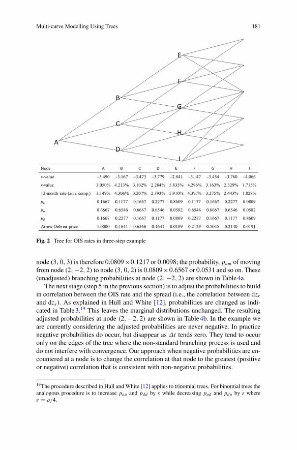
Discounting these values back to time 3Δt (= 1.5) gives the price of a one-yeardiscount bond at each node at 3Δt from which the bond’s yield can be determined.This is repeated for a bond that pays $1 at time 4Δt resulting in the one-year yields attime 2Δt , and so on. The tree constructed so far and the values calculated are shownin Fig. 2.18

The next stage (step 3 in the previous section) is to construct a tree for the spreadassuming that the expected future spread is zero (the preliminary tree). As in the caseof the OIS tree, Δt = 0.5 and Δy = σs

√3Δt = 0.2449. The branching process and

probabilities are calculated as for the OIS tree (with ar replaced by as).A three-dimensional tree is then created (step 4 in the previous section) by com-

bining the spread tree and the OIS tree assuming zero correlation. We denote thenode at time iΔt where x = jΔx and y = kΔy by node (i, j, k). Consider forexample node (2,−2, 2). This corresponds to node (2,−2) in the OIS tree, node Iin Fig. 2, and node (2, 2) in the spread tree. The probabilities for the OIS tree arepu = 0.0809, pm = 0.0583, pd = 0.8609 and the branching process is to nodeswhere j = 0, j = −1, and j = −2. The probabilities for the spread tree arepu = 0.1217, pm = 0.6567, pd = 0.2217 and the branching process is to nodeswhere k = 1, k = 2, and k = 3. Denote puu as the probability of the highest movein the OIS tree being combined with the highest move in the spread tree; pum as theprobability of the highest move in the OIS tree being combined with themiddle movein the spread tree; and so on. The probability, puu of moving from node (2,−2, 2) to

18More details on the construction of the tree can be found in Hull [10].


Fig. 2 Tree for OIS rates in three-step example

node (3, 0, 3) is therefore 0.0809×0.1217 or 0.0098; the probability, pum of movingfrom node (2,−2, 2) to node (3, 0, 2) is 0.0809×0.6567 or 0.0531 and so on. These(unadjusted) branching probabilities at node (2,−2, 2) are shown in Table4a.

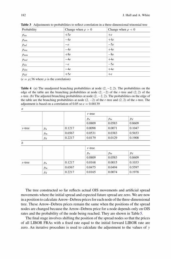
The next stage (step 5 in the previous section) is to adjust the probabilities to buildin correlation between the OIS rate and the spread (i.e., the correlation between dzrand dzs). As explained in Hull and White [12], probabilities are changed as indi-cated in Table3.19 This leaves the marginal distributions unchanged. The resultingadjusted probabilities at node (2,−2, 2) are shown in Table4b. In the example weare currently considering the adjusted probabilities are never negative. In practicenegative probabilities do occur, but disappear as Δt tends zero. They tend to occuronly on the edges of the tree where the non-standard branching process is used anddo not interfere with convergence. Our approach when negative probabilities are en-countered at a node is to change the correlation at that node to the greatest (positiveor negative) correlation that is consistent with non-negative probabilities.

19The procedure described in Hull and White [12] applies to trinomial trees. For binomial trees theanalogous procedure is to increase puu and pdd by ε while decreasing pud and pdu by ε whereε = ρ/4.


Table 3 Adjustments to probabilities to reflect correlation in a three-dimensional trinomial tree

Probability Change when ρ > 0 Change when ρ < 0

puu +5e +e

pum −4e +4e

pud −e −5e

pmu −4e +4e

pmm +8e −8e

pmd −4e +4e

pdu −e −5e

pdm −4e +4e

pdd +5e +e

(e = ρ/36 where ρ is the correlation)

Table 4 (a) The unadjusted branching probabilities at node (2,−2, 2). The probabilities on theedge of the table are the branching probabilities at node (2,−2) of the r -tree and (2, 2) of thes-tree. (b) The adjusted branching probabilities at node (2,−2, 2). The probabilities on the edge ofthe table are the branching probabilities at node (2,−2) of the r -tree and (2, 2) of the s-tree. Theadjustment is based on a correlation of 0.05 so e = 0.00139

a

r -tree

pu pm pd0.0809 0.0583 0.8609

s-tree pu 0.1217 0.0098 0.0071 0.1047

pm 0.6567 0.0531 0.0383 0.5653

pd 0.2217 0.0179 0.0129 0.1908

b

r -tree

pu pm pd0.0809 0.0583 0.8609

s-tree pu 0.1217 0.0168 0.0015 0.1033

pm 0.6567 0.0475 0.0494 0.5597

pd 0.2217 0.0165 0.0074 0.1978

The tree constructed so far reflects actual OIS movements and artificial spreadmovements where the initial spread and expected future spread are zero. We are nowin a position to calculateArrow–Debreu prices for each node of the three-dimensionaltree. These Arrow–Debreu prices remain the same when the positions of the spreadnodes are changed because the Arrow–Debreu price for a node depends only on OISrates and the probability of the node being reached. They are shown in Table5.

The final stage involves shifting the position of the spread nodes so that the pricesof all LIBOR FRAs with a fixed rate equal to the initial forward LIBOR rate arezero. An iterative procedure is used to calculate the adjustment to the values of y


Table 5 Arrow–Debreu prices for simple three-step example

i = 1 k = −1 k = 0 k = 1

j = 1 0.0260 0.1040 0.0342

j = 0 0.1040 0.4487 0.1040

j = −1 0.0342 0.1040 0.0260

i = 2 k = −2 k = −1 k = 0 k = 1 k = 2

j = 2 0.0004 0.0037 0.0089 0.0051 0.0008

j = 1 0.0045 0.0443 0.1064 0.0516 0.0061

j = 0 0.0112 0.1100 0.2620 0.1100 0.0112

j = −1 0.0061 0.0518 0.1070 0.0445 0.0046

j = −2 0.0008 0.0052 0.0090 0.0037 0.0004

i = 3 k = −3 k = −2 k = −1 k = 0 k = 1 k = 2 k = 3

j = 2 0.0001 0.0016 0.0085 0.0163 0.0109 0.0027 0.0002

j = 1 0.0005 0.0094 0.0496 0.0932 0.0551 0.0116 0.0007

j = 0 0.0012 0.0197 0.1016 0.1849 0.1016 0.0197 0.0012

j = −1 0.0008 0.0117 0.0557 0.0941 0.0501 0.0095 0.0005

j = −2 0.0002 0.0028 0.0111 0.0167 0.0087 0.0017 0.0001

at each node at each time step, β0, βΔt , β2Δt , . . . , so that the FRAs have a value ofzero. Given that Arrow–Debreu prices have already been calculated this is a fairlystraightforward search. When the α jΔt are determined it is necessary to first considerj = 0, then j = 1, then j = 2, and so on because the α-value at a particular timedepends on the α-values at earlier times. The β-values however are independent ofeach other and can be determined in any order, or as needed. In the case of ourexample, β0 = −6.493, βΔt = −6.459, β2Δt = −6.426, β3Δt = −6.395.

5 Valuation of a Spread Option

To illustrate convergence, we use the tree to calculate the value of a European calloption that pays off 100 times max(s − 0.002, 0) at time T where s is the spread.First, we let T = 1.5 years and use the three-step tree developed in the previoussection. At the third step of the tree we calculate the spread at each node. The spreadat node (3, j, k) is exp[φ(3Δt) + kΔy]. These values are shown in the second lineof Table6. Once the spread values have been determined the option payoffs, 100times max(s − 0.002, 0), at each node are calculated. These values are shown in therest of Table6. The option value is found by multiplying each option payoff by thecorrespondingArrow–Debreu price in Table5 and summing the values. The resultingoption value is 0.00670. Table7 shows how, for a 1.5- and 5-year spread option, thevalue converges as the number of time steps per year is increased.


Table 6 Spread and spread option payoff at time 1.5 years when spread option is evaluated usinga three-step tree

i = 3 k = −3 k = −2 k = −1 k = 0 k = 1 k = 2 k = 3

Spread 0.0008 0.0010 0.0013 0.0017 0.0021 0.0027 0.0035

j = 2 0.0000 0.0000 0.0000 0.0000 0.0133 0.0725 0.1482

j = 1 0.0000 0.0000 0.0000 0.0000 0.0133 0.0725 0.1482

j = 0 0.0000 0.0000 0.0000 0.0000 0.0133 0.0725 0.1482

j = −1 0.0000 0.0000 0.0000 0.0000 0.0133 0.0725 0.1482

j = −2 0.0000 0.0000 0.0000 0.0000 0.0133 0.0725 0.1482

Table 7 Value of a European spread option paying off 100 times the greater of the spread less0.002 and zero

Time steps per year 1.5-year option 5-year option

2 0.00670 0.0310

4 0.00564 0.0312

8 0.00621 0.0313

16 0.00592 0.0313

32 0.00596 0.0313

The market data used to build the tree is given in Tables1 and 2

Table 8 Value of a five-year European spread option paying off 100 times the greater of the spreadless 0.002 and zero

Spreadvolatility

Spread/OIS correlation

–0.75 –0.50 –0.25 0 0.25 0.5 0.75

0.05 0.0141 0.0142 0.0142 0.0143 0.0143 0.0144 0.0144

0.10 0.0193 0.0194 0.0195 0.0195 0.0196 0.0196 0.0197

0.15 0.0250 0.0252 0.0253 0.0254 0.0254 0.0255 0.0256

0.20 0.0308 0.0309 0.0311 0.0313 0.0314 0.0316 0.0317

0.25 0.0367 0.0369 0.0371 0.0373 0.0374 0.0376 0.0377

The market data used to build the tree are given in Tables1 and 2 except that the volatility of thespread and the correlation between the spread and the OIS rate are as given in this table. The numberof time steps is 32 per year

Table8 shows how the spread option price is affected by the assumed correlationand the volatility of the spread. All of the input parameters are as given in Tables1and 2 except that correlations between −0.75 and 0.75, and spread volatilities be-tween 0.05 and 0.25 are considered. As might be expected the spread option priceis very sensitive to the spread volatility. However, it is not very sensitive to the cor-relation. The reason for this is that changing the correlation primarily affects theArrow–Debreu prices and leaves the option payoffs almost unchanged. Increasingthe correlation increases the Arrow–Debreu prices on one diagonal of the final nodesand decreases them on the other diagonal. For example, in the three-step tree used


to evaluate the option, the Arrow–Debreu price for nodes (3, 2, 3) and (3,−2,−3)increase while those for nodes (3,−2, 3) and (3, 2,−3) decrease. Since the optionpayoffs at nodes (3, 2, 3) and (3,−2, 3) are the same, the changes on the Arrow–Debreu prices offset one another resulting in only a small correlation effect.

6 Bermudan Swap Option

We now consider how the valuation of a Bermudan swap option is affected by astochastic spread in a low-interest-rate environment such as that experienced in theyears following 2009. Bermudan swap options are popular instruments where theholder has the right to enter into a particular swap on a number of different swappayment dates.

The valuation procedure involves rolling back through the tree calculating boththe swap price and (where appropriate) the option price. The swap’s value is setequal to zero at the nodes on the swap’s maturity date. The value at earlier nodes iscalculated by rolling back adding in the present value of the next payment on eachreset date. The option’s value is set equal to max(S, 0) where S is the swap value atthe option’s maturity. It is then set equal to max(S, V ) for nodes on exercise dateswhere S is the swap value and V is the value of the option given by the roll backprocedure.

We assume an OIS term structure that increases linearly from 15 basis points attime zero to 250 basis points at time 10 years. The OIS zero rate for maturity t istherefore

0.0015 + 0.0235t

10

The process followed by the instantaneous OIS rate was similar to that derived byDeguillaume, Rebonato and Pogodin [7], and Hull and White [16]. For short ratesbetween 0 and 1.5%, changes in the rate are assumed to be lognormalwith a volatilityof 100%. Between 1.5% and 6% changes in the short rate are assumed to be normalwith the standard deviation of rate moves in time Δt being 0.015

√Δt . Above 6%

rate moves were assumed to be lognormal with volatility 25%. This pattern of theshort rate’s variability is shown in Fig. 3.

The spread between the forward 12-month OIS and the forward 12-month LIBORwas assumed to be 50 basis points for all maturities. The process assumed for the12-month LIBOR-OIS spread, s, is that used in the example in Sects. 4 and 5

dln(s) = as[φ(t) − ln(s)] + σs dzs


0.000

0.005

0.010

0.015

0.020

0.025

0.030

0.00% 2.00% 4.00% 6.00% 8.00% 10.00% 12.00%

s(r)

OIS short rate, r

Fig. 3 Variability assumed for short OIS rate, r , in Bermudan swap option valuation. The standarddeviation of the short rate in time Δt is s(r)

√Δt

Table 9 (a) Value in a low-interest rate environment, of a receive-fixed Bermudan swap option ona 5-year annual-pay swap where the notional principal is 100 and the option can be exercised attimes 1, 2, and 3 years. The swap rate is 1.5%. (b) Value in a low-interest-rate environment of areceived-fixed Bermudan swap option on a 10-year annual-pay swap where the notional principalis 100 and the option can be exercised at times 1, 2, 3, 4, and 5 years. The swap rate is 3.0%

Spreadvolatility

Spread/OIS correlation

a

–0.5 –0.25 –0.1 0 0.1 0.25 0.5

0 0.398 0.398 0.398 0.398 0.398 0.398 0.398

0.3 0.333 0.371 0.393 0.407 0.421 0.441 0.473

0.5 0.310 0.373 0.407 0.429 0.449 0.480 0.527

0.7 0.309 0.389 0.432 0.459 0.485 0.522 0.580

b

–0.5 –0.25 –0.1 0 0.1 0.25 0.5

0 2.217 2.218 2.218 2.218 2.218 2.218 2.218

0.3 2.100 2.164 2.201 2.225 2.248 2.283 2.339

0.5 2.031 2.141 2.203 2.242 2.280 2.335 2.421

0.7 1.980 2.134 2.218 2.271 2.321 2.392 2.503

Amaximum likelihood analysis of data on the 12-month LIBOR-OIS spread overthe 2012 to 2014 period indicates that the behavior of the spread can be approximatelydescribed by a high volatility in conjunction with a high reversion rate. We set asequal to 0.4 and considered values of σs equal to 0.30, 0.50, and 0.70. A number ofalternative correlations between the spread process and the OIS process were also


considered. We find that correlation of about −0.1 between one month OIS and the12-month LIBOR OIS spread is indicated by the data.20

We consider two cases:

1. A 3 × 5 swap option. The underlying swap lasts 5 years and involves 12-monthLIBOR being paid and a fixed rate of 1.5% being received. The option to enterinto the swap can be exercised at the end of years 1, 2, and 3.

2. A 5×10 swap option. The underlying swap lasts 10 years and involves 12-monthLIBOR being paid and a fixed rate of 3.0% being received. The option to enterinto the swap can be exercised at the end of years 1, 2, 3, 4, and 5.

Table9a shows results for the 3 × 5 swap option. In this case, even when thecorrelation between the spread rate and the OIS rate is relatively small, a stochasticspread is liable to change the price by 5–10%. Table9b shows results for the 5× 10swap option. In this case, the percentage impact of a stochastic spread is smaller.This is because the spread, as a proportion of the average of the relevant forwardOIS rates, is lower. The results in both tables are based on 32 time steps per year. Asthe level of OIS rates increases the impact of a stochastic spread becomes smaller inboth Table9a, b.

Comparing Tables8 and 9, we see that the correlation between the OIS rate andthe spread has a much bigger effect on the valuation of a Bermudan swap optionthan on the valuation of a spread option. For a spread option we argued that optionpayoffs for high Arrow–Debreu prices tend to offset those for low Arrow–Debreuprices. This is not the case for a Bermudan swap option because the payoff dependson the LIBOR rate, which depends on the OIS rate as well as the spread.

7 Conclusions

For investment grade companies it is well known that the hazard rate is an increasingfunction of time. This means that the credit spread applicable to borrowing by AA-rated banks from other banks is an increasing function of maturity. Since 2008,markets have recognized this with the result that the LIBOR-OIS spread has been anincreasing function of tenor.

Since 2008, practitioners have also switched from LIBOR discounting to OISdiscounting. This means that two zero curves have to bemodelled whenmost interestrate derivatives are valued. Many practitioners assume that the relevant LIBOR-OISspread is either constant or deterministic. Our research shows that this is liable tolead to inaccurate pricing, particularly in the current low interest rate environment.

The tree approach we have presented provides an alternative to Monte Carlosimulation for simultaneously modelling spreads and OIS rates. It can be regarded as

20Because of the way LIBOR is calculated, daily LIBOR changes can be less volatile than thecorresponding daily OIS changes (particularly if the Fed is not targeting a particular overnightrate). In some circumstances, it may be appropriate to consider changes over periods longer thanone day when estimating the correlation.


an extension of the explicit finite difference method and is particularly useful whenAmerican-style derivatives are valued. It avoids the need to use techniques such asthose suggested by Longstaff and Schwartz [19] and Andersen (2000) for handlingearly exercise within a Monte Carlo simulation.

Implying all the model parameters from market data is not likely to be feasible.One reasonable approach is to use historical data to determine the spread processand its correlation with the OIS process so that only the parameters driving the OISprocess are implied from the market. The model can then be used in the same waythat two-dimensional tree models for LIBOR were used pre-crisis.

Acknowledgements We are grateful to the Global Risk Institute in Financial Services for fundingthis research.

The KPMG Center of Excellence in Risk Management is acknowledged for organizing theconference “Challenges in Derivatives Markets - Fixed Income Modeling, Valuation Adjustments,Risk Management, and Regulation”.

Open Access This chapter is distributed under the terms of the Creative Commons Attribution4.0 International License (http://creativecommons.org/licenses/by/4.0/), which permits use, dupli-cation, adaptation, distribution and reproduction in any medium or format, as long as you giveappropriate credit to the original author(s) and the source, a link is provided to the Creative Com-mons license and any changes made are indicated.

The images or other third party material in this chapter are included in the work’s CreativeCommons license, unless indicated otherwise in the credit line; if such material is not includedin the work’s Creative Commons license and the respective action is not permitted by statutoryregulation, users will need to obtain permission from the license holder to duplicate, adapt orreproduce the material.

References

1. Ames,W.F.: NumericalMethods for Partial Differential Equations. Academic Press, NewYork(1977)

2. Anderson, L.: A simple approach to pricing Bermudan swap options in the multifactor LIBORmarket model. J. Comput. Financ. 3(2), 1–32 (2000)

3. Black, F., Derman, E., Toy, W.: A one-factor model of interest rates and its application totreasury bond prices. Financ. Anal. J. 46(1), 1–32 (1990)

4. Black, F., Karasinski, P.: Bond and option pricingwhen short rates are lognormal. Financ. Anal.J. 47(4), 52–59 (1991)

5. Brigo, D., Mercurio, F.: Interest Rate Models: Theory and Practice: With Smile Inflation andCredit, 2nd edn. Springer, Berlin (2007)

6. Collin-Dufresne, P., Solnik, B.: On the term structure of default premia in the swap and LIBORmarket. J. Financ. 56(3), 1095–1115 (2001)

7. DeGuillaume, N., Rebonato, R., Pogudin, A.: The nature of the dependence of the magnitudeof rate moves on the level of rates: a universal relationship. Quant. Financ. 13(3), 351–367(2013)

8. Hainaut, D., MacGilchrist, R.: An interest rate tree driven by a Lévy process. J. Deriv. 18(2),33–45 (2010)

9. Ho, T.S.Y., Lee, S.-B.: Term structure movements and pricing interest rate contingent claims.J. Financ. 41, 1011–1029 (1986)

10. Hull, J.: Options, Futures and Other Derivatives, 9th edn. Pearson, New York (2015)

http://creativecommons.org/licenses/by/4.0/


11. Hull, J., White, A.: Numerical procedures for implementing term structure models I. J. Deriv.2(1), 7–16 (1994)

12. Hull, J., White, A.: Numerical procedures for implementing term structure models II. J. Deriv.2(2), 37–48 (1994)

13. Hull, J., White, A.: Using Hull-White interest rate trees. J. Deriv. 3(3), 26–36 (1996)14. Hull, J.,White, A.: The general Hull-White model and super calibration. Financ. Anal. J. 57(6),

34–43 (2001)15. Hull, J., White, A.: LIBOR vs. OIS: The derivatives discounting dilemma. J. Invest. Manag.

11(3), 14–27 (2013)16. Hull, J., White, A.: A generalized procedure for building trees for the short rate and its ap-

plication to determining market implied volatility functions. Quant. Financ. 15(3), 443–454(2015)

17. Hull, J., White, A.: OIS discounting, interest rate derivatives, and the modeling of stochasticinterest rate spreads. J. Invest. Manag. 13(1), 13–20 (2015)

18. Kalotay, A.J., Williams, G.O., Fabozzi, F.J.: Amodel for valuing bonds and embedded options.Financ. Anal. J. 49(3), 35–46 (1993)

19. Longstaff, F.A., Schwartz, E.S.: ValuingAmerican options byMonteCarlo simulation: a simpleleast squares approach. Rev. Financ. Stud. 14(1), 113–147 (2001)

multi-curve modelling using trees - springer · pdf filemulti-curve modelling using trees ......

Documents