bootstrapping the ois curve in a south african bank

Univers

ityof

Cape T

own

Bootstrapping the OIS Curve in a South AfricanBank

Dirk van Heeswijk

A dissertation submitted to the Faculty of Commerce, University ofCape Town, in partial fulfilment of the requirements for the degree ofMaster of Philosophy.

September 7, 2017

MPhil in Mathematical Finance,University of Cape Town.

The copyright of this thesis vests in the author. No quotation from it or information derived from it is to be published without full acknowledgement of the source. The thesis is to be used for private study or non-commercial research purposes only.

Published by the University of Cape Town (UCT) in terms of the non-exclusive license granted to UCT by the author.

Univers

ity of

Cap

e Tow

n

Declaration

I declare that this dissertation is my own, unaided work. It is being submitted forthe Degree of Master of Philosophy in the University of the Cape Town. It has notbeen submitted before for any degree or examination in any other University.

September 7, 2017

Abstract

The financial crisis in 2007 highlighted the credit and liquidity risk present in in-terbank (LIBOR) rates, and resulted in changes to the pricing and valuation offinancial instruments. The shift to Overnight Indexed Swap (OIS) discountingand multi-curve framework led to changes in the construction of interest rate zerocurves, with the OIS curve being central to this methodology. Developed markets,such as the European (EUR), were able to adopt this framework due to the exis-tence of a liquid OIS market. In the case of the South African (ZAR) market, thelack of such tradeable instruments poses the issue of how to construct or infer theOIS curve. Jakarasi et al. (2015) proposed a method to infer the OIS curve throughthe statistical relationship between SAFEX ROD and 3M JIBAR. The extension ofthe statistical relationship used by Jakarasi et al. (2015) to more statistically rig-orous models, capable of capturing more information relating to the relationshipbetween the rates, arises from the expected cointegrating relationship exhibited be-tween rates. This dissertation investigates the implementation of such statisticalmodels to infer the OIS curve in the ZAR market.

Acknowledgements

There are many people I would like to thank for their contribution to this disser-tation. Obeid Mahomed for his guidance, knowledgeable input, and supervisionthroughout. Moorosi Mokhanoi and Tobias Hagstrom of FIS for the interestingand market relevant topic, as well as their valuable feedback. Andrea Macrina andGareth Peters of UCL for their insight into some areas of the dissertation. Lastly,my parents for enabling and supporting my education and this masters.

Contents

1. Introduction . . . . . . . . . . . . . . . . . . . . . . . . . . . . . . . . . . 1

2. Literature Review . . . . . . . . . . . . . . . . . . . . . . . . . . . . . . . 32.1 OIS Discounting . . . . . . . . . . . . . . . . . . . . . . . . . . . . . . . 32.2 Bootstrapping in Developed Markets . . . . . . . . . . . . . . . . . . . 3

2.2.1 OIS . . . . . . . . . . . . . . . . . . . . . . . . . . . . . . . . . . 32.2.2 LIBOR Curves under OIS Discounting . . . . . . . . . . . . . . 4

2.3 Bootstrapping in the ZAR Market . . . . . . . . . . . . . . . . . . . . . 62.4 Cointegration . . . . . . . . . . . . . . . . . . . . . . . . . . . . . . . . 7

2.4.1 Stationarity, Unit Root and Dickey-Fuller Tests . . . . . . . . . 72.4.2 Enlge-Granger Representation . . . . . . . . . . . . . . . . . . 82.4.3 Vector Autoregression (VAR), Vector Error Correction Model

(VECM) Representation . . . . . . . . . . . . . . . . . . . . . . 82.5 Cross Currency Implied OIS Curve . . . . . . . . . . . . . . . . . . . . 13

3. Statistical Analysis and Parameter Estimation . . . . . . . . . . . . . . . 143.1 Developed Markets - EUR . . . . . . . . . . . . . . . . . . . . . . . . . 14

3.1.1 Cointegrating Relationships . . . . . . . . . . . . . . . . . . . . 153.1.2 Parameter Estimation . . . . . . . . . . . . . . . . . . . . . . . 16

3.2 Developing Market - ZAR . . . . . . . . . . . . . . . . . . . . . . . . . 203.2.1 Cointegrating Relationship . . . . . . . . . . . . . . . . . . . . 203.2.2 Parameter Estimation . . . . . . . . . . . . . . . . . . . . . . . 21

3.3 Chapter Summary . . . . . . . . . . . . . . . . . . . . . . . . . . . . . . 24

4. Statistical Bootstrap Implementation and Results . . . . . . . . . . . . . 254.1 Developed Market . . . . . . . . . . . . . . . . . . . . . . . . . . . . . 25

4.1.1 Method . . . . . . . . . . . . . . . . . . . . . . . . . . . . . . . . 264.1.2 VECM Inferred . . . . . . . . . . . . . . . . . . . . . . . . . . . 284.1.3 OLSM Inferred . . . . . . . . . . . . . . . . . . . . . . . . . . . 304.1.4 Multivariate Cases . . . . . . . . . . . . . . . . . . . . . . . . . 32

4.2 ZAR Market . . . . . . . . . . . . . . . . . . . . . . . . . . . . . . . . . 364.2.1 Method . . . . . . . . . . . . . . . . . . . . . . . . . . . . . . . . 364.2.2 VECM Inferred . . . . . . . . . . . . . . . . . . . . . . . . . . . 374.2.3 OLSM Inferred . . . . . . . . . . . . . . . . . . . . . . . . . . . 38

4.3 Further Discussion and Extensions . . . . . . . . . . . . . . . . . . . . 414.4 Chapter Summary . . . . . . . . . . . . . . . . . . . . . . . . . . . . . . 41

5. Conclusion . . . . . . . . . . . . . . . . . . . . . . . . . . . . . . . . . . . 43

Bibliography . . . . . . . . . . . . . . . . . . . . . . . . . . . . . . . . . . . . 45

A. Boostrapping Instruments . . . . . . . . . . . . . . . . . . . . . . . . . . 47

v

List of Figures

3.1 EUR historical reference rates . . . . . . . . . . . . . . . . . . . . . . . 143.2 EUR EONIA residuals vs. observed for entire data set . . . . . . . . . 193.3 ZAR historical reference rates . . . . . . . . . . . . . . . . . . . . . . . 203.4 ZAR SAFEX ROD residuals vs. observed for entire data set . . . . . . 23

4.1 EUR market implied zero curves . . . . . . . . . . . . . . . . . . . . . 264.2 EUR VECM inferred OIS curves and daily rate forecasts . . . . . . . . 284.3 EUR OLSM inferred OIS curves and daily rate forecasts . . . . . . . . 304.4 EUR OLS inferred OIS curve at the short end . . . . . . . . . . . . . . 324.5 EUR multivariate OLSM inferred OIS curves . . . . . . . . . . . . . . 334.6 ZAR VECM daily rate forecasts . . . . . . . . . . . . . . . . . . . . . . 374.7 ZAR OLSM inferred OIS curves and daily rate forecasts . . . . . . . . 38

vi

List of Tables

3.1 EUR maximum eigenvalue test statistics . . . . . . . . . . . . . . . . . 153.2 EUR Maximum eigenvalue test statistics - multivariate post-crisis . . 153.3 EUR ADF test statistics . . . . . . . . . . . . . . . . . . . . . . . . . . . 173.4 EUR OLSM parameters . . . . . . . . . . . . . . . . . . . . . . . . . . . 173.5 EUR residual ADF test statistics . . . . . . . . . . . . . . . . . . . . . . 173.6 EUR VECM parameters . . . . . . . . . . . . . . . . . . . . . . . . . . 183.7 EUR rates ARCH test . . . . . . . . . . . . . . . . . . . . . . . . . . . . 193.8 ZAR maximum eigenvalue test statistics . . . . . . . . . . . . . . . . . 213.9 ZAR ADF test statistics . . . . . . . . . . . . . . . . . . . . . . . . . . . 213.10 ZAR OLSM parameters . . . . . . . . . . . . . . . . . . . . . . . . . . 223.11 ZAR ADF test statistics . . . . . . . . . . . . . . . . . . . . . . . . . . . 223.12 ZAR VECM parameters . . . . . . . . . . . . . . . . . . . . . . . . . . 223.13 ZAR rates ARCH test . . . . . . . . . . . . . . . . . . . . . . . . . . . . 23

4.1 EUR OLSM inferred OIS against market implied . . . . . . . . . . . . 314.2 EUR multivariate OLSM inferred OIS rates against market implied . 344.3 EUR multivariate spread between OLSM inferred and market implied 354.4 EUR SSE ×104 . . . . . . . . . . . . . . . . . . . . . . . . . . . . . . . . 364.5 ZAR OLSM inferred OIS against 3M JIBAR . . . . . . . . . . . . . . . 40

A.1 EUR OIS Market Instruments . . . . . . . . . . . . . . . . . . . . . . . 48A.2 EUR 1M Market Instruments . . . . . . . . . . . . . . . . . . . . . . . 48A.3 EUR 3M Market Instruments . . . . . . . . . . . . . . . . . . . . . . . 49A.4 EUR 6M Market Instruments . . . . . . . . . . . . . . . . . . . . . . . 49A.5 EUR 12M Market Instruments . . . . . . . . . . . . . . . . . . . . . . . 50A.6 ZAR 3M Market Instruments . . . . . . . . . . . . . . . . . . . . . . . 51

vii

Chapter 1

Introduction

Since the financial crisis in 2007, significant attention has been drawn to the dis-count rates and methods used when valuing financial instruments. Prior to thecrisis, the assumption that highly rated banks did not run the risk of default led tothe use of LIBOR rates as a proxy for the risk-free rate. The relationship and negligi-ble spread between LIBOR and OIS rates supported this assumption, and allowedfor the use of the single-curve framework for the pricing and valuation of financialinstruments (i.e. no consideration was given to the different tenors of LIBOR asso-ciated with each market instrument, and both forecasting and discounting used asingle LIBOR curve).

During the crisis, it was observed that banks and other highly rated financialinstitutions could default on payments. This led to spreads between the differenttenor LIBOR and OIS rates widening, based on credit and liquidity premiums at-tached to each tenor (Clarke, 2010c). Noting that each tenor LIBOR had uniquecredit and liquidity risk premiums, a single forecasting curve could not explainsuch differences, thus requiring unique forecasting curves for each tenor LIBOR.Furthermore, under the collateralisation of transactions, the collateral posted ontransactions earned the reference overnight rate, which was forecasted and dis-counted using the OIS curve. Hence, the OIS curve was adopted as the discountingcurve for such transactions. These factors led to the implementation of the multi-curve framework, with the OIS rates used as the discounting rates, and differenttenor LIBOR rates as the respective forecasting rates. This multi-curve frameworkhas been implemented in most developed markets, due to the existence of a liquidOIS market.

When considering the case of the ZAR market, it is evident that the market lacksa tradeable overnight rate (Jakarasi et al., 2015). Whilst there exist overnight refer-ence rates, such as SAFEX ROD and SABOR, no instruments trade on these rates.This prevents the construction of the fundamental OIS curve. In addition, the lackof liquid market instruments with different tenor JIBAR hampers the implementa-

Chapter 1. Introduction 2

tion of a complete multi-curve framework. Jakarasi et al. (2015) proposed a statis-tical method to infer the OIS curve, under the assumption that LIBOR (3M JIBAR)and OIS (SAFEX ROD) rates exhibit a cointegrating relationship. This serves as ba-sis for the use of statistical methods to infer relationships between rates, with theextension to models such as the vector-error correction model (VECM) of interestdue to the cointegrating relationships.

The focus of this dissertation is thus to identify and implement a method ofbootstrapping the OIS curve used to correctly discount collateralised transactionsin the ZAR market. The use of statistical methods to accomplish the above is in-vestigated, with implementation in a developed (EUR) market allowing for therobustness and performance of the models to be tested. An outline of the researchaims and considerations are highlighted below:

1. Identification of current methods used to imply/bootstrap the OIS curve frommarket instruments. Develop an understanding of the implementation ofsuch procedures in a developed market (EUR), including the construction ofthe curve using current bootstrapping methods.

2. Determination of the statistical relationship between LIBOR and OIS rates,using historical reference rate data, in both the EUR and ZAR markets. Iden-tification of cointegrating relationships and estimation of statistical model pa-rameters using the Johansen and Engle-Granger procedures are of interest.

3. Implementation of the statistical model in a bootstrapping procedure in boththe EUR and ZAR markets, identifying the need for different methods undersingle- and multi-curve frameworks. Ascertain the validity of the statisticallyinferred OIS curves by comparison to the current market method. Investigatethe implied OIS curves under multivariate cases in the EUR market, under-standing the influence of the number and tenor of rates used in the models.

Chapter 2

Literature Review

2.1 OIS Discounting

Under the post-crisis setting and Credit Support Annex (CSA), the collateralizationof transactions was implemented to reduce the risk of counterparty default. Clarke(2010c) and Hull and White (2013) note that the collateral posted earns interestat the overnight reference rate. As the collateral must reflect the current mark tomarket value of the transaction, Clarke (2010c) highlights that this overnight refer-ence rate must be used to discount future expected cashflows on such collateralizedtransactions to satisfy no arbitrage.

Given the widespread use of OIS discounting, the need to bootstrap the OIScurve is fundamental to correct valuation of transactions.

2.2 Bootstrapping in Developed Markets

Developed markets, such as EUR, were quick to adopt the multi-curve framework,with the use of OIS discounting. The existence of an actively traded overnight ratewas fundamental to the implementation of this methodology.

2.2.1 OIS

The OIS curve is constructed under the single-curve framework, as the curve isused to both forecast and discount cash flows. The standard instrument is that ofthe OIS, with the simple fair swap rate Ro(t0, ti) given by,

Ro(t0, tn) =1

τ

[n∏

i=1

(1 +Do(ti−1, ti)τi)− 1

](2.1)

where

• τ is the year fraction from t0 to tn

2.2 Bootstrapping in Developed Markets 4

• τi is the year fraction from ti−1 to ti

• Do(ti−1, ti) is the simple overnight reference rate that applies for the i-th busi-ness day

Clarke (2010b) highlights an alternate method of bootstrapping the short-endof the OIS curve. Daily compounding of overnight reference rates is used to con-struct the curve out over the short-end (under the assumption that the referencerate will remain largely unchanged for certain periods, in line with market dynam-ics and expectations). Under such a framework, interpolation between dates onthe short-end is not viable, as the step-function of the reference rates could lead tosignificant errors (i.e. when interpolated over a step). The construction of the mid-and long-end then uses the market available OIS rates, with the use of interpolationto determine intermediate rates (as per the standard bootstrapping procedure).

For the purposes of the dissertation, the standard single-curve framework willbe used to bootstrap the market OIS curve, with no consideration to the method ofClarke (2010b) for the short-end. This is left as a possible extension to the disserta-tion. The particular OIS instruments used in the EUR market are given in AppendixA.

2.2.2 LIBOR Curves under OIS Discounting

Ametrano and Bianchetti (2009) propose a method for multi-curve discounting andbootstrapping, a brief overview of which is given for reference. The method in-volves firstly constructing a single discounting curve (the OIS curve as per the ar-guments above). Thereafter homogeneous LIBOR market instruments (referencingLIBOR rates with the same underlying tenor) are selected, based on availabilityand liquidity. Finally, the yield curves for each of the respective tenors can be con-structed by forecasting cashflows with these homogeneous LIBOR market rates anddiscounting these cashflows with the OIS curve.

For the purpose of this dissertation, only cash deposit-, forward rate agreement-, and swap rates will be used in the bootstrapping procedure. Furthermore, theserates associated with these instruments were assumed to be deterministic. Thespecific market instruments used to bootstrap each of the diferent tenor LIBORcurve can be found in Appendix A.

Cash Deposit

The cash deposit (DEP) rate is the simple rate corresponding to the interest a partywill earn when depositing cash for a given maturity. The equivalent NACC zerorate rx(t0, tn) for tenor x is given by,

2.2 Bootstrapping in Developed Markets 5

rx(t0, tn) =1

τln(1 + Lx(t0, tn)τ) (2.2)

where


• Lx(t0, tn) is the respective tenor simple market rate

Forward Rate Agreement

A forward rate agreement (FRA) is the interest a party will earn on a deposit start-ing at some point in the future tj , for a given maturity tn. When using these instru-ments for bootstrapping, it is important to note that the tenor of the FRA (differencebetween near and far dates) must coincide with the tenor of the zero curve beingbootstrapped. The equivalent NACC zero rate rx(t0, tn) for tenor x is given by,

rx(t0, tn) =fx(t0; tj , tn)τn + rx(t0, tj)τj

τ(2.3)

where


• τj is the year fraction from t0 to tj

• τn is the year fraction from tj to tn

• fx(t0; tj , tn) is the fair NACC forward rate

Interest Rate Swap

Swap (SWP) rates are the fair rate at which a party can exchange floating LIBORpayments over a number of tenor periods, for a given given maturity tn. The equiv-alent simple floating LIBOR rate for the final reset period Lx(tn−1, tn) is given by,

Lx(tn−1, tn) =

Kxn∑

i=1τiZ

o(t0, ti)−n−1∑i=1

Lx(ti−1, ti)τiZo(t0, ti)

τnZo(t0, tn)(2.4)

2.3 Bootstrapping in the ZAR Market 6

where

• Kx is the fair swap rate for the respective tenor swap

• τi is the year fraction from t0 to ti

• Zo(t0, ti) is the discount factor for ti, determined from the discounting (OIS)curve

This expected tenor LIBOR rate can then be used to determine the equivalentNACC zero rate rx(t0, tn).

2.3 Bootstrapping in the ZAR Market

In the ZAR market, there exists no tradable overnight rate. Whilst there existovernight reference rates, such as SAFEX ROD and SABOR, no instruments tradeon these rates (i.e. no OIS instruments). As a result, there is no readily availableOIS curve that can be used as a proxy for the risk-free rate.

Jakarasi et al. (2015) propose a method for bootstrapping the ZAR OIS curvethrough the assumption of a cointegrating relationship between the SAFEX RODand 3M JIBAR. 3M JIBAR was selected based on it being the most liquid tenortraded in the ZAR market, and the SAFEX ROD rate was used above that of theSABOR as the overnight reference rate, based on the characteristics and construc-tion of each rate. Jakarasi et al. (2015) begin by determining the realised floatingOIS rate for a given tenor (3M given the liquidity of interbank rates in the ZARmarkets). Thereafter, the cointegration relationship between the floating OIS rateand interbank rate of corresponding tenor (3M JIBAR) is calculated, allowing forthe simultaneous bootstrapping of the OIS and JIBAR curves.

Jakarasi et al. (2015) propose two Engle-Granger cointegration models for the3M floating OIS rate (3M FL), using the 3M JIBAR rate (3M JIBAR) and 3M JIBAR-SAFEX spread (SPD). The two models are as follows,

(3M FL)t = β1(3M JIBAR)t + β2(SPD)t + α, (2.5)

(3M FL)t = β1(3M JIBAR)t + α. (2.6)

The first model takes into consideration both the above mentioned instruments/indices,with the second model considering only the 3M JIBAR rate. In addition, whenchecking the robustness of the models on developed markets, Jakarasi et al. (2015)found that the first model performed better on long dated swaps, with the second

2.4 Cointegration 7

model performing better on short dated swaps. This led to the proposal of a hybridmodel, using the LIBOR rate and SPD model for the short-end and the LIBOR onlymodel for the long-end.

The work of Jakarasi et al. (2015) shows that the modeling of the OIS rate usinga cointegration based approach produces reasonable results.

2.4 Cointegration

Cointegration is used to describe the relationship between to variables or processesthat appear to have a common long run trend. Engle and Granger (1987) show thatgiven two or more integrated/non-stationary I(1) variables, such that some linearcombination of the variables is stationary I(0), then the variables can be consideredto exhibit a cointegrating relationship.

2.4.1 Stationarity, Unit Root and Dickey-Fuller Tests

An integrated non-stationary I(1) series contains one unit root, such that when dif-ferenced the series is stationary I(0). This is shown by considering the process

yt = ρyt−1 + ut, (2.7)

where ut is a stationary process, such that

∆yt = (ρ− 1)yt−1 + ut. (2.8)

Banerjee et al. (1993) highlight that for ∆yt to be stationary, we require ρ = 1 (i.e.the series contains one unit root). In checking a univariate time series for stationar-ity, the null hypothesis of H0 : ρ = ρ0 = 1 is tested. Ordinary least squares (OLS)regression is used to estimate the test statistic ρ, which is then used to construct thetest statistic,

ρ− ρ0SE(ρ)

(2.9)

Banerjee et al. (1993) further note that ρ has a non-asymptotic, non-symmetricaldistribution. As a result, it is compared to critical values, tabulated by Dickey andFuller (1979).

2.4 Cointegration 8

2.4.2 Enlge-Granger Representation

Engle and Granger (1987) proposed a two-step procedure to identify and determinethe cointegrating relationship between variables. Given two time series variablesxt, yt, the processes must first be tested for the existence of a unit root suchthat both can be confirmed to be integrated I(1). This allows for the application ofthe Dickey-Fuller test discussed above. Having confirmed non-stationarity of theprocesses, and under the assumption of a cointegrating relationship, the followingregression is considered,

yt = βxt + vt, (2.10)

where vt contains stationary I(0) dynamics. OLS regression can then be used toestimate β, under the omission of vt,

β =

(T∑t=1

xtyt

)(T∑t=1

x2t

)−1(2.11)

The residual estimates, vt = yt−βxt, are then tested for stationarity, again usingthe Dickey-Fuller tests. Should the residuals vt prove to be stationarity, the nullhypothesis of a cointegrating relationship cannot be rejected and the variables canbe assumed to be cointegrated. Under the Engle-Granger approach, the estimatescan then be extended to the error correction model. This is achieved through theinclusion of stationary terms, such as autoregressive components (based on theADF test) and lagged cointegrating relationships. This dissertation will use theJohansen procedure to estimate the VECM model, with the Engle-Granger OLSregression above of interest based on the its application by Jakarasi et al. (2015).

Should the residuals prove to be non-stationary, the variables can not be con-sidered to exhibit a cointegrating relationship. This leads to a case of spuriousregression, with the VECM and OLSM unable to correctly capture the relationship.

2.4.3 Vector Autoregression (VAR), Vector Error Correction Model(VECM) Representation

A vector autoregressive (VAR) model can be used to describe the interrelationshipbetween two (or more) stationary variables and the previous values of each of thevariables. The VECM representation of a VAR process allows for the interrelation-ship between two (or more) variables that are stationary in the first differences tobe determined, again based on the previous values of the first differences of thevariables. Furthermore, the VECM representation allows for the determination

2.4 Cointegration 9

of a cointegration relationship between the variables, as shown by Johansen andJuselius (1990).

Engle and Granger (1987) derive the error correction model (ECM) for an n-dimensional vector autoregressive process (VAR) of order p. The notation and rep-resentation follows that of Johansen and Juselius (1990).

∆XXXt = ΠΠΠXXXt−1 +

p−1∑i=1

ΓΓΓi∆XXXt−i + ΦΦΦDDDt +µµµ+ εεεt (2.12)

where

• ΠΠΠ is the long-run multiplier matrix

• ΓΓΓi is the ith lag matrix

• φφφ is a matrix

• DDDt is a vector of deterministic terms

• εεεt is independent identically distributed multivariate, correlated errors

From Johansen and Juselius (1990) and Banerjee et al. (1993), the nature of therelationship between the variables is dependent on the rank of the long-run multi-plier matrix, rank(ΠΠΠ) = r. For the case of r = 0, no cointegration exists betweenthe variables, and the relationship should be respecified as vector autoregressive infirst differences i.e. VAR(p − 1). For the case of r = n, the variables are stationary,i.e. VAR(p) model is stable. Finally, for the case of 0 < r < n, a cointegration rela-tionship exists between the variables. Under such conditions, ΠΠΠ can be split into theloading matrix ααα and cointegrating matrix βββ, with both ααα and βββ of size n× r, suchthat ΠΠΠ = αααβββ′. Furthermore, it is noted that the decomposition of ΠΠΠ is not unique.

Johansen Procedure

The Johansen procedure allows for the determination of the model parameters ofthe VECM. Rearranging Equation 2.12, by Johansen and Juselius (1990) we havethe following form of the VECM:

ZZZ0t = ΠΠΠZZZkt + ΓΓΓZZZ1t + εεεt (2.13)

where

• ZZZ0t = ∆XXXt

• ZZZkt = XXXt−k

2.4 Cointegration 10

• ZZZ1t denotes the stacked variables [∆XXXt−1, . . . ,∆XXXt−k+1,DDDt,111]′

• ΓΓΓ denotes the parameters [ΓΓΓ1, ...,ΓΓΓk−1,ΦΦΦ,µµµ]

Johansen and Juselius (1990) highlights the method of solving for the modelparameters, by maximising the log likelihood function. The following derivation ofthe estimation of cointegrating vectors follows Banerjee et al. (1993), with notationconsistent with that of (Johansen and Juselius, 1990). Starting with the general formof the VECM in Equation 2.12, excluding deterministic terms DDDt, the distributionof the erros εεεt are assumed to follow a multivariate normal distribution,

εεεt ∼ N(0,Ω0,Ω0,Ω). (2.14)

From the multivariate normal distribution, the log-likelihood function can be de-rived,

L(ΓΓΓ1, ...,ΓΓΓk−1,ΠΠΠ,ΩΩΩ|(XXX1, ...,XXXT )) =− Tn2

log(2π)− T

2log |ΩΩΩ|

− 1

2

T∑t=1

εεε′tΩΩΩ−1εεεt.

(2.15)

ConcentrateL(ΓΓΓ1, ...,ΓΓΓk−1,ΠΠΠ,ΩΩΩ|(XXX1, ...,XXXT )) with respect to ΩΩΩ followed (ΓΓΓ1, ...,ΓΓΓk−1)

in order to reduce the likelihood function to L∗(ΠΠΠ).This is achieved by lettingZZZkt = XXXt−k andZZZt1 = (∆XXX ′t−1, ...,∆XXX

′t−k+1)

′, and usingregression to partial out the effect of ZZZkt and ZZZt1 on (ΓΓΓ1, ...,ΓΓΓk−1). The residualsRRR0t,RRRkt are defined as,

RRR0t = ∆XXXt −k−1∑i=1

ΓΓΓi∆XXXt−i (2.16)

where

(ΓΓΓ1, ..., ΓΓΓk−1) =

(T∑t=1

∆XXXtZZZ′t1

)(T∑t=1

∆ZZZt1ZZZ′t1

)−1, (2.17)

and

RRRkt = XXXt−k −k−1∑i=1

ΓΓΓi∆XXXt−i (2.18)

where

(ΓΓΓ1, ..., ΓΓΓk−1) =

(T∑t=1

∆XXXt−kZZZ′t1

)(T∑t=1

ZZZt1ZZZ′t1

)−1. (2.19)

Thus, the concentrated likelihood function L∗(ΠΠΠ) is given,


L∗(ΠΠΠ) = K − T

2log

∣∣∣∣∣T∑t=1

(RRR0t −ΠΠΠRRRkt)(RRR0t −ΠΠΠRRRkt)′

∣∣∣∣∣ . (2.20)

The second moment matrices and cross-products can then be determined from theresidualsRRR0t,RRRkt,

SSSij =1

T

T∑t=1

RRRitRRR′jt, i, j = 0, k. (2.21)

Rewriting Equation 2.20,

L∗(ΠΠΠ) = K0 −T

2log∣∣SSS00 −ΠΠΠSSSk0 −SSS0kΠΠΠ

′ + ΠΠΠSSSkkΠΠΠ′∣∣ . (2.22)

The restriction ΠΠΠ = αααβββ′ is now imposed on the system, giving

L∗(ααα,βββ) = K0 −T

2log∣∣SSS00 −αααβββ′SSSk0 −SSS0kβββααα

′ +αααβββ′SSSkkβββααα′∣∣ . (2.23)

Next, L∗(ααα,βββ) is further concentrated with respect to ααα, giving an expression forthe MLE of ααα as a function of βββ, and a concentrated likelihood function dependingon βββ. From Equation 2.23,

∂L∗(ααα,βββ)

∂ααα= 0, (2.24)

giving

ααα = SSS0kβββ(βββ′SSSkkβββ)−1. (2.25)

Substituting the above into Equation 2.23,

L∗∗(βββ) = K1 −T

2log∣∣SSS00 −SSS0kβββ(βββ′SSSkkβββ)−1βββ′SSSk0

∣∣ . (2.26)

Differentiating L∗∗(βββ) with respect to βββ is achieved by applying partitioned inver-sion results,

∣∣SSS00 −SSS0kβββ(βββ′SSSkkβββ)−1βββ′SSSk0

∣∣ =∣∣βββ′SSSkkβββ

∣∣−1 |SSS00|∣∣βββ′SSSkkβββ − βββ′SSSk0SSS

−100 SSS0kβββ

∣∣=∣∣βββ′SSSkkβββ

∣∣−1 |SSS00|∣∣βββ′(SSSkk −SSSk0SSS

−100 SSS0k)βββ

∣∣ . (2.27)

Noting that maximising L∗∗(βββ) with respect to βββ corresponds to minimising thegeneralised variance ratio, with |SSS00| constant,∣∣βββ′(SSSkk −SSSk0SSS

−100 SSS0k)βββ

∣∣|βββ′SSSkkβββ|

. (2.28)


Under the normalisation βββ′SSSkkβββ = I , this results in the minimisation of,∣∣βββ′(SSSkk −SSSk0SSS−100 SSS0k)βββ

∣∣ . (2.29)

This reduces to solving the eigenvalue problem

(λλλSSSkk −SSSk0SSS

−100 SSS0k

)βββ = 0 (2.30)

∣∣λλλSSSkk −SSSk0SSS−100 SSS0k

∣∣ = 0 (2.31)

for largest eigenvalues λ1 ≥ λ2 ≥ ... ≥ λr ≥ λn ≥ 0

Giving βββ = (vvv1, vvv2, ..., vvvr) of the corresponding eigenvectors. The remaining pa-rameters are obtained by solving backwards as functions of the MLE of βββ.

The results of the parameter estimation are dependent on the correct estimationof the number of cointegrating relationships (i.e. the cointegration rank) Johansenand Juselius (1990); Banerjee et al. (1993). Two well-known tests associated with theJohansen procedure are that of the trace test and maximum eigenvalue test. It isproposed that the maximum eigenvalue test will be used, thus the trace test willnot be discussed further. For the maximum eigenvalue test, the null hypothesisHr,is tested against the alternative Hr+1, with the likelihood ratio test statistic

ζr = −T ln(1− λr+1), r = 0, 1, ..., n− 1. (2.32)

The above test statistic is compared against the limiting distribution, as per Jo-hansen (1995), to accept or reject the hypotheses. See Johansen and Juselius (1990)or Banerjee et al. (1993) for a detailed discussion of the VECM and above procedure.

Heteroskedasticity and the Autoregressive Conditional Heteroskedastic(ARCH) Test

Heteroskedasticity is the condition whereby the variance of a process is not con-stant over time. When considering a statistical model, such as that of OLS, changesin the variance of fitted values with observed values is a strong indication of het-eroskedasticity. Engle (1982) proposed the ARCH class of models, along with theARCH test. As the ARCH model is not considered, and heteroskedasticity and theARCH test do not have a major influence on the aims or results of this dissertation,the concepts are introduced for reference only. See Engle (1982) for a more detaileddiscussion of heteroskedasticity and the ARCH test.

2.5 Cross Currency Implied OIS Curve 13

2.5 Cross Currency Implied OIS Curve

The use of foreign exchange (FX) instruments to bootstrap a domestic (ZAR) OIScurve can be considered on the basis that the collateral could be posted in the for-eign (EUR) market. The existence of an OIS curve and different tenor LIBOR curvesin the EUR market, along with multiple liquid FX instruments for ZAR-EUR, allowsfor the ZAR OIS curve to be implied through these FX market instruments.

White (2012) highlights the use of FX instruments to determine the discountingcurve in one currency (ZAR), given the existence of such a curve in the other cur-rency (EUR). The construction of the short-end of the OIS curve is based on forwardexchange rates, with the long-end based on cross currency basis swaps (floating forfloating). Knowing the EUR OIS curve, along with a set of EUR and ZAR tenor LI-BOR curves (such as 3M LIBOR/JIBAR), the ZAR OIS curve can be implied. Clarke(2010a) provides further insight and justification for the use of FX instruments, con-sistent with that of White (2012). As with the above, this requires the existence of adiscounting curve in the currency/market (EUR) in which the collateral is posted.Clarke (2010a) shows that some swap, when valued using the unknown (ZAR) dis-count curve, should price to a fair value VZ . This can be converted to EUR at thespot exchange rate, giving VE (the collateral amount). This VE is then invested atthe EUR collateral rate (OIS rate) to the ZAR swap cash flow dates, and convertedback to ZAR using forward foreign exchange rates. Thus the ZAR discount curveshould present value the cash flows to fair swap value, allowing the ZAR discountcurve to be determined given the existence of the required instruments and rates.The use of forward foreign exchange rates is viable up to 1 year, after which crosscurrency basis swaps should be used.

When considering the use of FX instruments, it is important to note the exis-tence of an associated country risk-premium. This premium results in the corre-sponding OIS curve being recovered at a premium to the true OIS curve, inducingcredit and liquidity risk components that are not unique to the OIS rate. As a result,this method of implying the OIS curve will not be considered in this dissertation,with methods capable of implying a clean OIS curve being preferred.

Chapter 3

Statistical Analysis and ParameterEstimation

Statistical analyses were performed on EUR (EONIA, 1M, 3M, 6M, 12M) and ZAR(SAFEX ROD, 3M JIBAR) reference rates, over the period 01 January 2000 - 31 De-cember 2015. The data set was further broken into to pre- and post-crisis periods, toexamine the influence of the different characteristics of each period. The pre-crisisperiod was 1 January 2000 - 31 July 2007, and the post-crisis period 1 July 2009 -31 December 2015. All tests were run at the 1% significance level with the numberof lags set to 0, where applicable. The main aims of the analyses were to check forthe existence of cointegrating relationships, and estimate the parameter values foreach of the statistical models.

3.1 Developed Markets - EUR

The historical data for the EUR market is shown in Figure 3.1.

2001 2002 2003 2004 2005 2006 2007 2008 2009 2010 2011 2012 2013 2014 2015-0.01

0

0.01

0.02

0.03

0.04

0.05

0.06

EONIA1M EURIBOR3M EURIBOR6M EURIBOR12M EURIBOR

Fig. 3.1: EUR historical reference rates

3.1 Developed Markets - EUR 15

3.1.1 Cointegrating Relationships

Of the methods and models discussed in Chapter 2, the VECM and Johansen proce-dure were used to test the historical EUR rates data for cointegrating relationships.The cointegration rank was examined through the use of the maximum eigenvaluetest statistics, with these given in Table 3.1 (1% critical test values are given forreference). If the test statistic was found to be greater than the critical, the nullhypothesis of cointegration of that rank could be rejected.

It can be seen from Table 3.1 that there exists cointegration between EUR rates.The entire data set exhibits cointegration rank 3, pre-crisis rank 4, and post-crisisrank 3.

Tab. 3.1: EUR maximum eigenvalue test statistics

Data Set Cointegration Rank0 1 2 3 4

1% Critical Values 39.3693 32.7172 25.8650 18.5200 6.6349Entire 595.7623 228.1295 54.2363 8.9552 2.3721Pre-crisis 460.5301 152.8202 76.3340 27.4817 3.9490Post-crisis 394.1090 192.0820 67.6369 5.2034 2.8228

Multivariate Cases

In order to establish if the results were influenced by the number of variates (rates)included in the analysis, the tests were repeated for different multivariate cases.This was done using the entire data set only. Table 3.2 shows the maximum eigen-value test statistics against the 1% critical values.

Tab. 3.2: EUR Maximum eigenvalue test statistics - multivariate post-crisis

Data Set Cointegration Rank (Lowest - Highest)

1% Critical Values 39.3693 32.7172 25.8650 18.5200 6.6349EONIA-1M 350.9166 1.6443EONIA-3M 186.6138 2.1466EONIA-1M-3M 503.9676 18.1250 1.8647EONIA-3M-6M 462.2516 35.9075 1.8149EONIA-1M-3M-6M 535.9252 219.5935 7.5986 2.0001EONIA-3M-6M-12M 498.4087 89.1419 18.6970 2.0142


In the EUR market, when considering the bivariate cases, it was found thatthere exists cointegration of rank 1. The tri-variate cases show cointegration ofrank 2 in the case of EONIA-3M-6M, yet only rank 1 in the case of EONIA-1M-3M. It was noted that the test statistic lies close to the critical value for the lattercase. The quad-variate cases provide further insight, with the case of EONIA-1M-3M-6M and exhibiting rank 2, and EONIA-3M-6M-12M exhibiting cointegrationof rank 3. Due to each of the multivariate cases exhibiting strong cointegrationrelationships, it was found that it may not be necessary to include all rates in thecointegration/statistical model. If one considers the historical data for the post-crisis world, it can be seen that the different tenored rates appear to shifted versionsof one another (see Figure 3.1), thus including all tenors may not provide additionalinformation in terms of the cointegrating relationship.

3.1.2 Parameter Estimation

Parameter estimates are presented for both the Engle-Granger regression model(henceforth referred to as OLSM) and VECM. Estimates are given for the case ofall LIBOR rates, over the entire, pre-crisis, and post-crisis data sets. Note that inthe case of the VECM, the parameter estimates take into consideration the order ofcointegration.

OLSM

The Engle-Granger procedure discussed in Chapter 2 was used to estimate theOLSM parameters. The augmented Dickey-Fuller test was performed to check forstationarity (or non-stationarity) of the variables.

ADF test statistics for each of the EUR rates are reported in Table 3.3, with thecritical value at the 1% level -2.568 for each case. In order to reject the null hy-pothesis, a test statistic lower than that of the critical value was required. It wasfound that in all cases the null hypothesis was unable to be rejected, indicatingthe existence of a unit root and non-stationarity of the rates. The one exception tothe above was that of the post-crisis EONIA, however the increased volatility overparts of this time period could lead to a poor test statistic and result. Based on vi-sual inspection and the non-stationarity of the different LIBOR tenors, it was thusassumed that the post-crisis EONIA data was also non-stationary.


Tab. 3.3: EUR ADF test statistics

EONIA 1M 3M 6M 12M

Entire -1.0509 1.1749 1.9046 1.8760 1.5204Pre -1.0025 -1.3144 -1.4905 -1.2657 -0.7970Post -3.8808 1.3163 3.1816 3.7445 3.2882

Having established non-stationarity of the rate processes, the parameter esti-mates for the EUR OLSM, of the form OIS = β11M + β23M + β36M + β412M + β0,were estimated by OLS regression. These values are shown in Table 3.4. It wasfound that the OLSM assigned different weightings to different tenor LIBOR rateswhen considering each of the data sets. These weightings can be interpreted asholdings in each of the tenor LIBOR rates, such that the net holding replicates along position of 1 in the OIS rate. Furthermore, it was noted that for each dataset significant holdings were required in the 1M and 3M tenor LIBOR rates, withsmaller holdings in the 6M and 12M tenor LIBOR rates.

Tab. 3.4: EUR OLSM parameters

Entire Pre-crisis Post-crisis

β1

β2

β3

β4

β0

1.8405

−1.5264

1.1312

−0.4600

0.0003

1.3818

−0.0181

−0.4637

0.1052

−0.0004

1.4969

−1.8267

1.0283

0.0237

−0.0007

Lastly, in order to confirm that the rates were correctly modeled as cointegrated,the residual values were checked for stationarity using the ADF test as above. Ta-ble 3.5 shows that for each of the data sets the null hypothesis of a unit root wasstrongly rejected, indicating that the residuals were stationary and the OLS wasvalid.

Tab. 3.5: EUR residual ADF test statistics

EONIA

Entire -21.6562Pre -20.4708Post -17.6935


VECM

Having performed the Johansen procedure in checking for cointegrating relation-ships, the parameter estimates were recovered and examined. As the Johansenprocedure was run with no lags, only the estimates for the ααα and βββ parameters areshown. Comparison of these parameters allows for some insight into the impact ofthe choice of data set, due to the fact that ααα and βββ constitute the long run relation-ship and this is of key importance when considering the performance of the VECM.Note the parameter estimates shown in Table 3.6 are in matrix form.

Tab. 3.6: EUR VECM parameters

ααα× 10−3 βββ × 103

Enti

re

0.3256 0.1038 0.0273

0.0274 −0.0372 0.0077

0.0333 −0.0267 −0.0043

0.0352 −0.0277 −0.0052

0.0374 −0.0285 −0.0126

−0.5537 −0.2490 −0.0461

0.7640 1.1766 −0.5860

−0.4440 −1.8533 3.1068

0.7746 0.7226 −4.3720

−0.5653 0.2380 1.8804

Pre

0.4546 0.0524 0.0336 −0.0065

0.0022 −0.0420 0.0054 −0.0031

0.0201 −0.0439 −0.0038 −0.0051

0.0243 −0.0463 0.0116 −0.0095

0.0270 −0.0461 0.0183 −0.0249

−0.7463 −0.1392 0.0252 −0.0189

0.9979 −0.1400 −2.7274 0.4097

0.1700 −0.1677 5.7156 1.5705

−0.4458 0.2726 −3.7282 −3.8712

0.0287 0.1778 0.7023 1.9109

Post

−0.2878 −0.1723 −0.0279

−0.0199 0.0117 0.0066

−0.0169 0.0130 0.0012

−0.0133 0.0120 −0.0005

−0.0122 0.0114 0.0001

0.8094 0.5052 0.1072

−0.0806 −2.4485 −0.8544

−0.4552 3.4741 3.1613

−0.0462 −1.5886 −1.6994

0.0480 0.0482 −0.4109

From Table 3.6 it can be seen that the parameters do not vary significantly interms of the magnitude of the values, however there are differences across the datasets. Differences in the signs of parameters can be explained by the different trendsover the respective periods. Any variation in the parameters can be explained bythe different nature of the rates over the entire data set, with the rates pre-crisishaving a notably different nature to those of the post-crisis. This suggests that thetime period over which the parameters are estimated should be considered in orderto produce the better estimates.

Real world interpretation of the VECM parameters proves challenging, as these


correspond to holdings in the daily rate changes and lagged realisations of the dif-ferent tenor LIBOR rates.

In particular, the general trend of the rates over a given time period has a sig-nificant impact on the parameters. General upward or downward trends give riseto different signs, along with values to which the rates will converge towards inthe long-run. The impact of the above will discussed in more detail in followingsections, with the application of the VECM to forecasting rates.

Heteroskedasticity

In order to check for heteroskedasticity in each of the models, the residuals wereplotted against the observed values, and the ARCH test was performed on all resid-uals. The ARCH test statistics were compared to the critical value of 6.6349, withvalues above indicating rejection of the null hypothesis of no ARCH effects.

-0.010 0.000 0.010 0.020 0.030 0.040 0.050 0.060

Observed Values

-0.015

-0.010

-0.005

0.000

0.005

0.010

Res

idua

l Val

ues

(a) VECM

-0.010 0.000 0.010 0.020 0.030 0.040 0.050 0.060

Observed Values

-0.015

-0.010

-0.005

0.000

0.005

0.010

0.015

Res

idua

l Val

ues

(b) OLS

Fig. 3.2: EUR EONIA residuals vs. observed for entire data set

Tab. 3.7: EUR rates ARCH test

VECM OLSData Set EONIA 1M 3M 6M 12M EONIA

Entire 315.2512 0.7697 10.8252 34.0722 34.9072 2369.8269Pre-crisis 112.2798 3.3939 0.9393 5.4914 14.8794 431.8585Post-crisis 286.8176 7.0360 1.3828 0.4520 0.1859 413.0432

Figures 3.2a and 3.2b show no noticeable increase in the variance (greater dis-persion of residuals) with observed values, thus it cannot be concluded that therates exhibit heteroskedasticity.

3.2 Developing Market - ZAR 20

The ARCH test, Table 3.7, highlighted the existence of heteroskedasticity, withall tests relating to EONIA rejecting the null hypotheses that there exist no ARCHeffects. The existence of heteroskedasticity can be in part explained by the differ-ence in volatility between rates and the existence of periods of greater/less volatil-ity, seen in Figure 3.1. Whilst the existence of heteroskedasticity does weaken thecointegrating relationship, it does not invalidate the use of cointegrating relation-ships and the VECM. With regard to the OLSM, the existence of heteroskedasticitydoes result in the OLSM estimates no longer being the most efficient, however theyremain unbiased. Due to the nature of the rates, it was accepted that heteroskedas-ticity would always exist to some extent and thus no changes were made to themodels or method of parameter estimation.

3.2 Developing Market - ZAR

The historical data for the ZAR market is shown in Figure 3.3.

2001 2002 2003 2004 2005 2006 2007 2008 2009 2010 2011 2012 2013 2014 20150.04

0.05

0.06

0.07

0.08

0.09

0.1

0.11

0.12

0.13

0.14

SAFEX ROD3M JIBAR

Fig. 3.3: ZAR historical reference rates

3.2.1 Cointegrating Relationship

As was the case with the EUR market, the VECM and Johansen procedure was usedto check for a cointegrating relationship between the ZAR rates. The maximumeigenvalue test statistics for the ZAR data are reported in Table 3.8.

It was observed that over all time periods SAFEX ROD and 3M JIBAR are coin-tegrated with rank 1. This was as expected and allowed for a cointegration basedbootstrapping procedure to be used.


Tab. 3.8: ZAR maximum eigenvalue test statistics

Data Set Cointegration Rank0 1

1% Critical Values 18.5200 6.6349Entire 316.8702 1.7505Pre-crisis 144.7263 1.6313Post-crisis 31.2864 0.0000

3.2.2 Parameter Estimation

The parameter estimates are presented for each model, over the entire, pre-crisis,and post-crisis data sets. Note that in the case of the VECM, the parameter esti-mates take into consideration the order of cointegration.

OLSM

The parameter estimation for the OLSM followed the procedure used in the EURmarket.

ADF test statistics for the ZAR rates are reported in Table 3.9. Given the nullhypothesis of the existence of a unit root, it was found that in all cases we wereunable to reject the null hypothesis, indicating that the rates are non-stationary.

Tab. 3.9: ZAR ADF test statistics

SAFEX ROD 3M

Entire 0.8434 1.5281Pre 0.3195 0.5204Post 0.9340 0.9157

Having established non-stationarity of the rate processes, the parameters for theZAR OLSM, of the form OIS = β13M + β0, were estimated using OLS regression.These estimates are shown in Table 3.10. As with the EUR market, the parameter β1corresponds to a long holding in 3M JIBAR (noting a fractional holding is requiredin order to replicate a long position of 1 in the OIS rate). It was found that these pa-rameters agree with those estimated by Jakarasi et al. (2015), thus further validatingthe potential implementation of the model.


Tab. 3.10: ZAR OLSM parameters

Entire Pre-crisis Post-crisis

β1

β0

0.9729

−0.00201175

0.9487

0.00057655

0.9300

−0.00003709

Lastly, the residual values were tested for stationarity. Table 3.11 shows the teststatistics for each of the data sets. It can be seen that in all cases the null hypothesisof a unit root was rejected, implying stationarity of the residuals and the cointe-grating relationship under the OLSM was validated.

Tab. 3.11: ZAR ADF test statistics

SAFEX ROD

Entire -6.7714Pre -4.5884Post -3.0953

VECM

The parameter estimates for the VECM are shown in Table 3.12. Only estimates forααα and βββ are shown, with each taking into consideration the order of cointegration.It can be seen that as with the EUR market, the estimates vary with the data set.Note as with the EUR case, parameter estimates are given in matrix form, and realworld interpretation of the parameters proves challenging due to the form of theVECM.

Tab. 3.12: ZAR VECM parameters

ααα× 103 βββ × 10−3

Enti

re 0.0522

0.1152

0.3809

−0.3697

Pre 0.0508

0.1210

0.3405

−0.3215

Post 0.0134

0.0263

1.0796

−0.9761


Heteroskedasticity

In order to check for heteroskedasticity, the residuals were plotted against the fittedvalues, and the ARCH test was performed on all residuals. The ARCH test statisticswere compared to the critical value of 6.6349, with values above indicating rejectionof the null hypothesis.

Figure 3.4 shows the residual values against the observed values for both theVECM and OLSM. It can be seen from Figure 3.4a that the residuals for the VECMexhibit clustering, however no increase in variance with observed values is visible.The clustering are a result of the the stepped nature of the post-crisis 3M JIBAR andSAFEX ROD as seen in Figure 3.3. Furthermore, the residuals from rate change areclearly noticeable. In contrast, Figure 3.4b clearly shows changes in the variance ofresiduals with observed values, indicating heteroskedasticity.

0.040 0.050 0.060 0.070 0.080 0.090 0.100 0.110 0.120 0.130

Observed Values

-0.010

-0.005

0.000

0.005

0.010

0.015

0.020

Res

idua

l Val

ues

(a) VECM

0.040 0.050 0.060 0.070 0.080 0.090 0.100 0.110 0.120 0.130

Observed Values

-0.010

-0.005

0.000

0.005

0.010

0.015

0.020

Res

idua

l Val

ues

(b) OLS

Fig. 3.4: ZAR SAFEX ROD residuals vs. observed for entire data set

Tab. 3.13: ZAR rates ARCH test

VECM OLSData Set SAFEX ROD 3M SAFEX ROD

Entire 0.0124 0.0365 3354.1578Pre-crisis 0.0024 0.0003 1634.6713Post-crisis 0.0349 0.0088 1414.6205

The ARCH test results, as seen in Table 3.13, confirmed the observations madein above using Figure 3.4, with the VECM residuals exhibiting no heteroskedas-ticity (unable to reject null hypothesis) and the OLSM residuals exhibiting het-eroskedasticity (rejection of the null hypothesis).

3.3 Chapter Summary 24

3.3 Chapter Summary

The Johansen procedure was used to examine the nature of the relationship be-tween reference rates within markets. It was found that there exists a cointegratingrelationship between rates in all markets tested. Furthermore, when consideringmultivariate cases (of different combinations of rates) it was found that the cointe-grating relationships still exist. This supports the possibility of a statistical modelwith less covariates being used to describe the relationship still producing reason-able results.

Parameters were recovered using the Johansen procedure and OLS regression,and the estimates over different data sets were compared. It was found that the pa-rameters do change when considering different periods, due to differences in thegeneral trend of the rates over the given period. In particular, general upward ordownward trends alter the signs of the parameter estimates, the impact of whichwas found to be significant. This highlights the need for consideration into the dataused to estimate model parameters when implementing the statistical models. Realworld interpretation of the parameters is reasonable in the case of the OLSM, withthe parameters representing long and short positions in each of the tenor LIBORrates (noting fractional holdings are required). In the case of the VECM, interpre-tation proves challenging as the parameters represent holdings in the day to daydifferences and lagged realisations of the tenor LIBOR rates, potentially unattain-able in a market setting.

In order to further understand the relationship, the residuals were tested forheteroskedasticity. This was done by examining residual plots and performing anARCH test on the residuals. Under the VECM, it was found that heteroskedasticityexists to some extent in the EUR market but not in the ZAR market. Under theOLSM, it was found that heteroskedasticity exists in both the EUR and ZAR market.Due to the nature of rates, with OIS exhibiting greater variance and changes invariance over time, these effects are hard to mitigate or remove and are thus onlynoted for reference.

Chapter 4

Statistical BootstrapImplementation and Results

The implementation of the statistical relationships determined in the Chapter 3 al-lowed for the OIS and different tenor LIBOR zero curves to be bootstrapped fromthe respective LIBOR market instruments. All bootstrapping took place assumingZAR business days (for both EUR and ZAR market cases), using raw interpolationwhere required, and for 16 July 2015.

4.1 Developed Market

The developed market presented a combination of challenges when attemptingto bootstrap the OIS curve. The underlying cause of which was the multicurveframework, which results in market prices being derived under OIS discountingand the respective tenor LIBOR forecasting. However these same LIBOR curveswere required to infer the OIS curve using the statistical relationships determinedin Chapter 3. These challenges resulted in the need to simultaneously bootstrapthe OIS and different tenor LIBOR curves. As a baseline result, the OIS and LIBORcurves were bootstrapped under the current market method, with the zero curvesshown in Figure 4.1.

4.1 Developed Market 26

Jan-2016 Jan-2026 Jan-2036 Jan-2046 Jan-2056-5

0

5

10

15

20×10-3

12M6M3M1MOIS

Fig. 4.1: EUR market implied zero curves

4.1.1 Method

It was noted that even under the multi-curve framework, the DEP and FRA zerorates could be bootstrapped independently of the OIS curve. This allowed for thestandard bootstrapping procedure to be applied to these instruments, requiringonly the SWP rates to be simultaneously bootstrapped. The simultaneous boot-strapping procedure developed is detailed below.

1. Identify the market instruments and rates to be used in the bootstrappingprocedure for each tenor LIBOR, along with the initial visible OIS referencerate

2. Bootstrap the DEP and FRA zero rates for each of the different tenor LIBORcurves, and set up ’dummy’ rates for each of the SWP zero rates such that aninitial guess of each of the tenor LIBOR curves is obtained

3. (VECM only) Using the market visible and previously realised OIS and tenorLIBOR reference rates, initialise the VECM forecasting model

4. For the following business day, imply each of the different tenor LIBOR for-ward rates, using the current guess for each of the tenor LIBOR zero curves

5. Apply the statistical model (VECM/OLSM) to forecast the OIS rate for the


given business day, using the above forward LIBOR rates as the expectedvalue of the tenor LIBOR reference rates

6. Stepping through each of the successive business days, out till the end of thezero curve, imply each of the successive forward LIBOR rates and infer thecorresponding OIS rates

7. From the successive daily forecasts of the OIS rate, recover the OIS zero curve(see Equation 2.1)

8. Using this inferred OIS curve and estimated LIBOR curves, recover each ofthe SWP zero rates under the multi-curve pricing framework

9. Repeat until convergence is obtained for the each of the SWP zero rates

The simultaneous multi-curve bootstrapping procedure required that each ofthe different tenor LIBOR curves be estimated at each convergence iteration, in or-der to allow for the OIS curve to be inferred. Thereafter, all of the required SWPzero rates (corresponding to all swaps of all LIBOR tenors) were repriced. This en-sured convergence of the system as a whole for a given set of market rates, inferredOIS curve, and tenor LIBOR curves.

Furthermore, it was noted that the OIS curve obtained from the above proce-dure was limited by the shortest maturity LIBOR curve, minus the longest tenorof LIBOR rate used. For example, if the 1M curve extended out to 30 years, and12M was the longest tenor LIBOR rate used, then the OIS curve would extend outto 29 years. This was due to the fact that in order to estimate the OIS rate at a givenpillar date, each tenor forward LIBOR rate was required at that pillar date, thusrequiring a LIBOR zero curve that extended the respective tenor beyond the pillardate. Furthermore, at each convergence iteration this required the last SWP rateto be estimated, such that the full tenor LIBOR curve could be recovered. As theOIS curve would not extend to this last pillar date, it was not possible to recoverthe rate under OIS discounting. The proposed solution was to bootstrap each thelast tenor SWP rates under the single-curve framework, as simply using the marketvisible fair swap rate as an estimate for the zero rate was highly inaccurate.


4.1.2 VECM Inferred

The following results are those of the VECM inferred OIS curve in the EUR market.In order to investigate the influence of the data set, and corresponding parameters,the procedure was implemented using both the entire and post-crisis data set.


0

2

4

6

8

10

12

14

16

18×10-3

MarketVECM

(a) OIS curves: entire data set

Jan-2016 Jan-2026 Jan-2036-0.005

0

0.005

0.01

0.015

0.02

0.025

0.03

12M6M3M1MOIS

(b) Daily rate forecasts: entire data set


0

2

4

6

8

10

12

14

16

18×10-3

MarketVECM

(c) OIS curves: post-crisis data set

Jan-2016 Jan-2026 Jan-2036-0.005

0

0.005

0.01

0.015

0.02

0.025

0.03

12M6M3M1MOIS

(d) Daily rate forecasts: post-crisis data set

Fig. 4.2: EUR VECM inferred OIS curves and daily rate forecasts

Figure 4.2 shows the VECM inferred OIS curves and daily rate forecasts forboth the entire and post-crisis data set, with the market implied OIS curve givenfor reference in each case. Figures 4.2a and 4.2c show the impact of the data set andparameters on the results of the inferred OIS curves. Under the entire data set, theinferred OIS curve was able to capture the correct term structure, and appeared tobe a shifted version of the market implied OIS curve. Under the post-crisis dataset, the VECM relationship was unable to capture the correct term structure, failingto infer any reasonable OIS curve. The shifted OIS curve visible in Figure 4.2a


was a result of the autoregressive component of the VECM. The dependence ofOIS forecasts on previous forecasts reduces the ability of the VECM to capture theterm structure, as this term structure was visible only in the forward LIBOR rates.The contribution of this autoregressive component, which was compounded by thenumber of successive daily forecasts, was enough to offset the OIS curve from thatof the market implied OIS curve.

The VECM parameters, specifically the long run relationship, had a significantimpact on the daily forecasts of the OIS rate. In Figure 4.2d, the under estimationof the daily OIS rates is visible. As in the post-crisis world there exists noticeablespread between OIS and different tenor LIBOR rates, when this spread starts todecrease, and forward LIBOR rates converge, the relationship produces poor esti-mates for the OIS rate. When considering the entire data set, the existence of thepre-crisis period with little or no spread between different tenor LIBOR rates allowsfor the OIS forecasts to be less effected by the decreasing spread visible in forwardLIBOR rates. The decreasing spread visible in forward LIBOR rates indicates thepossibility that future LIBOR rates will no longer maintain the post-crisis spreadlevels, returning to a state similar to that of the pre-crisis period. When implement-ing the VECM, the parameters are designed to capture long-term trends, and thusspecific data sets with unique characteristics (such as the spread observed in thepost-crisis period) should not be used.


4.1.3 OLSM Inferred

The following of results are those of the OLSM implied OIS curve in the EUR mar-ket. As was the case with the VECM, the influence of the data set was investigated.


0

2

4

6

8

10

12

14

16

18×10-3

MarketOLS


Jan-2016 Jan-2026 Jan-2036-0.005

0

0.005

0.01

0.015

0.02

0.025

0.03

12M6M3M1MOIS



0

2

4

6

8

10

12

14

16

18×10-3

MarketOLS


Jan-2016 Jan-2026 Jan-2036-0.005

0

0.005

0.01

0.015

0.02

0.025

0.03

12M6M3M1MOIS


Fig. 4.3: EUR OLSM inferred OIS curves and daily rate forecasts

Figure 4.3 shows the OLSM inferred OIS curves and daily rate forecasts forboth the entire and post-crisis data set, with the market implied OIS curve givenfor reference in each case. Under the entire data set, Figure 4.3a shows that the OLSinferred OIS curve appeared to coincide with that of the market implied OIS curve.Under the post-crisis data set however, Figure 4.3c shows the OLSM implied OIScurve was unable to correctly capture the required term structure. This failure ofthe post-crisis OLSM can be attributed to the same shortcomings of the post-crisisVECM discussed above, with Figure 4.3d clearly showing the under estimation ofthe daily OIS rates.


Tab. 4.1: EUR OLSM inferred OIS against market implied

Date Market implied (%) OLSM (%) Spread (bps)

17-Jul-2015 -0.1220 -0.1240 -0.200023-Jul-2015 -0.1210 -0.0872 3.382317-Aug-2015 -0.1200 -0.0746 4.543116-Sep-2015 -0.1220 -0.0973 2.474116-Oct-2015 -0.1255 -0.1118 1.372616-Nov-2015 -0.1270 -0.1160 1.096517-Dec-2015 -0.1300 -0.1212 0.882518-Jan-2016 -0.1300 -0.1239 0.611016-Feb-2016 -0.1320 -0.1278 0.422316-Mar-2016 -0.1340 -0.1333 0.072718-Apr-2016 -0.1350 -0.1377 -0.269316-May-2016 -0.1370 -0.1410 -0.402517-Jun-2016 -0.1380 -0.1427 -0.472218-Jul-2016 -0.1380 -0.1419 -0.388316-Aug-2016 -0.1372 -0.1399 -0.265216-Sep-2016 -0.1364 -0.1362 0.013217-Oct-2016 -0.1355 -0.1326 0.288516-Nov-2016 -0.1347 -0.1290 0.567619-Dec-2016 -0.1338 -0.1257 0.809416-Jan-2017 -0.1330 -0.1229 1.013118-Apr-2017 -0.1239 -0.1121 1.180417-Jul-2017 -0.1151 -0.1071 0.795616-Jul-2018 -0.0440 -0.0521 -0.805316-Jul-2019 0.0741 0.0571 -1.699916-Jul-2020 0.2178 0.2065 -1.127816-Jul-2021 0.3621 0.3504 -1.164918-Jul-2022 0.5132 0.5184 0.516917-Jul-2023 0.6565 0.6458 -1.069116-Jul-2024 0.7873 0.7600 -2.731816-Jul-2025 0.9067 0.8761 -3.060216-Jul-2026 1.0134 0.9728 -4.061916-Jul-2027 1.1114 1.0737 -3.773016-Jul-2030 1.3266 1.2937 -3.291316-Jul-2035 1.5210 1.4971 -2.387216-Jul-2040 1.5787 1.5549 -2.377318-Jul-2044 1.5964 1.5882 -0.8285


Jan-2016 Jan-2017 Jan-2018 Jan-2019 Jan-2020 Jan-2021-20

-15

-10

-5

0

5×10-4

MarketOLS

Fig. 4.4: EUR OLS inferred OIS curve at the short end

Table 4.1 shows the OLSM inferred and market implied NACC rates for a givenset of pillar dates, along with the basis point spread between the two. The mini-mal spread between rates confirmed the performance of the OLSM, with no spreadgreater than 5 bps in both the short- and long-end. The reason for the improved per-formance over the VECM was that the OLSM was able to imply the OIS rate andterm structure directly from the forward LIBOR rates, with no further influencefrom long run relationships or autoregressive components. Minor divergence be-tween the OLSM and market implied OIS curves occurs only in the extreme short-and long-end. The reason for the long-end divergence was that the last maturitySWP rate was bootstrapped under the single-curve framework, with the need todo so previously discussed. Divergence in the short-end, as seen in Figure 4.4,was a result of the forecasting under the statistical relationship, with the shortend of different tenor LIBOR curves having to be estimated using the same set ofnon-homogeneous rates. These non-homogeneous rates do not show the expectedspread between different tenor LIBOR, and thus would not fit the statistical modelparameters as estimated.

4.1.4 Multivariate Cases

Having established that there exist cointegrating relationships even when consid-ering fewer tenor LIBOR rates, and that the OLSM was capable of recovering themarket implied OIS curve, the impact of the implementation of these different mul-tivariate cases was investigated. It was reasoned that shorter tenor LIBOR rates,


such as 1M and 3M, would be more closely related to the OIS rate, as a result of lesscredit and liquidity risk. Given the improved performance of the OLSM under theentire data set, multivariate cases were considered only under this model.

2016 2021 2026 2031 2036 2041 2046 2051 2056 2061-2

0

2

4

6

8

10

12

14

16

18×10-3

MarketOLS

(a) EONIA-1M

2016 2021 2026 2031 2036 2041 2046 2051 2056 2061-2

0

2

4

6

8

10

12

14

16

18×10-3

MarketOLS

(b) EONIA-3M

2016 2021 2026 2031 2036 2041 2046 2051 2056 2061-2

0

2

4

6

8

10

12

14

16

18×10-3

MarketOLS

(c) EONIA-1M-3M

2016 2021 2026 2031 2036 2041 2046 2051 2056 2061-2

0

2

4

6

8

10

12

14

16

18×10-3

MarketOLS

(d) EONIA-1M-3M-6M

Fig. 4.5: EUR multivariate OLSM inferred OIS curves

From Figure 4.5 it can be seen that the number of LIBOR rates included in thestatistical model had a noticeable impact. The bivariate cases seen in Figures 4.5aand 4.5b perform worse than that of the tri- and quad variate cases, seen in Figures4.5c and 4.5d respectively. Furthermore, the case of OIS-3M performs worse thanthat of OIS-1M, whilst the tri- and quad variate cases appear to perform better thanthat of the full multivariate case, suggesting that certain rates are more closely re-lated to the OIS rate. This was confirmed when considering Tables 4.2 and 4.3, withthe basis spread being relatively low for each of the selected curve dates. Further-more, it was found that the case of EONIA-1M performed best in the short-end ofthe curve, with the the tri- and quad-variate cases performing noticeably better inthe long-end.


Tab. 4.2: EUR multivariate OLSM inferred OIS rates against market implied

Date Market implied (%) 1M (%) 3M (%) 1M-3M (%) 1M-3M-6M (%)

17-Jul-2015 -0.1220 -0.1240 -0.1240 -0.1240 -0.124023-Jul-2015 -0.1210 -0.1380 -0.1969 -0.0798 -0.086217-Aug-2015 -0.1200 -0.1305 -0.2016 -0.0619 -0.068916-Sep-2015 -0.1220 -0.1409 -0.2030 -0.0779 -0.085716-Oct-2015 -0.1255 -0.1471 -0.2044 -0.0878 -0.095916-Nov-2015 -0.1270 -0.1483 -0.2053 -0.0892 -0.097217-Dec-2015 -0.1300 -0.1500 -0.2060 -0.0915 -0.099418-Jan-2016 -0.1300 -0.1515 -0.2075 -0.0929 -0.100616-Feb-2016 -0.1320 -0.1533 -0.2081 -0.0957 -0.103216-Mar-2016 -0.1340 -0.1550 -0.2065 -0.0992 -0.106918-Apr-2016 -0.1350 -0.1562 -0.2046 -0.1022 -0.110016-May-2016 -0.1370 -0.1573 -0.2030 -0.1050 -0.112917-Jun-2016 -0.1380 -0.1573 -0.2012 -0.1067 -0.114718-Jul-2016 -0.1380 -0.1564 -0.1995 -0.1069 -0.114916-Aug-2016 -0.1372 -0.1554 -0.1964 -0.1072 -0.115216-Sep-2016 -0.1364 -0.1543 -0.1930 -0.1074 -0.115217-Oct-2016 -0.1355 -0.1533 -0.1897 -0.1076 -0.114916-Nov-2016 -0.1347 -0.1518 -0.1864 -0.1070 -0.114319-Dec-2016 -0.1338 -0.1501 -0.1828 -0.1063 -0.113616-Jan-2017 -0.1330 -0.1487 -0.1798 -0.1058 -0.112018-Apr-2017 -0.1239 -0.1411 -0.1698 -0.0988 -0.104117-Jul-2017 -0.1151 -0.1333 -0.1601 -0.0956 -0.100616-Jul-2018 -0.0440 -0.0630 -0.0756 -0.0361 -0.040316-Jul-2019 0.0741 0.0493 0.0502 0.0656 0.061316-Jul-2020 0.2178 0.1899 0.1963 0.2011 0.197516-Jul-2021 0.3621 0.3416 0.3500 0.3499 0.346818-Jul-2022 0.5132 0.4922 0.4988 0.5005 0.499017-Jul-2023 0.6565 0.6345 0.6390 0.6432 0.640416-Jul-2024 0.7873 0.7666 0.7678 0.7765 0.772816-Jul-2025 0.9067 0.8833 0.8817 0.8940 0.890016-Jul-2026 1.0134 0.9834 0.9841 0.9923 0.987616-Jul-2027 1.1114 1.0835 1.0771 1.0957 1.090516-Jul-2030 1.3266 1.2954 1.2751 1.3157 1.310516-Jul-2035 1.5210 1.4828 1.4463 1.5132 1.507916-Jul-2040 1.5787 1.5367 1.4881 1.5750 1.568218-Jul-2044 1.5964 1.5628 1.4969 1.6009 1.5936


Tab. 4.3: EUR multivariate spread between OLSM inferred and market implied

Date 1M (bps) 3M (bps) 1M-3M (bps) 1M-3M-6M (bps)

17-Jul-2015 -0.2000 -0.2000 -0.2000 -0.200023-Jul-2015 -1.7046 -7.5935 4.1227 3.478117-Aug-2015 -1.0526 -8.1625 5.8140 5.114016-Sep-2015 -1.8868 -8.0990 4.4059 3.631016-Oct-2015 -2.1591 -7.8854 3.7709 2.965516-Nov-2015 -2.1340 -7.8251 3.7765 2.981117-Dec-2015 -1.9980 -7.5956 3.8501 3.059418-Jan-2016 -2.1475 -7.7475 3.7057 2.942516-Feb-2016 -2.1330 -7.6077 3.6337 2.881616-Mar-2016 -2.0947 -7.2452 3.4834 2.714918-Apr-2016 -2.1207 -6.9602 3.2764 2.497716-May-2016 -2.0256 -6.6034 3.1975 2.409617-Jun-2016 -1.9266 -6.3240 3.1291 2.330818-Jul-2016 -1.8361 -6.1503 3.1082 2.307216-Aug-2016 -1.8180 -5.9158 3.0057 2.205216-Sep-2016 -1.7987 -5.6651 2.8962 2.115617-Oct-2016 -1.7793 -5.4144 2.7866 2.062916-Nov-2016 -1.7101 -5.1719 2.7664 2.040319-Dec-2016 -1.6340 -4.9051 2.7441 2.013516-Jan-2017 -1.5694 -4.6787 2.7252 2.098918-Apr-2017 -1.7145 -4.5891 2.5140 1.981017-Jul-2017 -1.8172 -4.5014 1.9457 1.445716-Jul-2018 -1.8930 -3.1558 0.7947 0.373416-Jul-2019 -2.4831 -2.3958 -0.8557 -1.288016-Jul-2020 -2.7860 -2.1452 -1.6748 -2.025416-Jul-2021 -2.0534 -1.2127 -1.2160 -1.524818-Jul-2022 -2.1068 -1.4402 -1.2763 -1.423917-Jul-2023 -2.1945 -1.7517 -1.3286 -1.609316-Jul-2024 -2.0655 -1.9524 -1.0801 -1.445216-Jul-2025 -2.3419 -2.4949 -1.2693 -1.669416-Jul-2026 -2.9995 -2.9302 -2.1082 -2.578216-Jul-2027 -2.7959 -3.4363 -1.5677 -2.091216-Jul-2030 -3.1249 -5.1543 -1.0892 -1.607716-Jul-2035 -3.8154 -7.4693 -0.7811 -1.310216-Jul-2040 -4.1952 -9.0619 -0.3717 -1.049418-Jul-2044 -3.3622 -9.9527 0.4434 -0.2835

4.2 ZAR Market 36

To further measure the performance of the OLSM, the sum of squared errors(SSE) was calculated for each curve. This compared each of the inferred OIS zerorates to the market implied zero rates, for each business day included in the zerocurve, providing a more complete view of the performance of each of the EUROLSM cases. Note that for all multivariate cases, only points up to the maturity co-inciding with that of the full EUR OLSM were considered. These errors confirmedthe performance of the different multivariate cases, with the EONIA-1M-3M hav-ing the lowest SSE, followed closely by the EONIA-1M-3M-6M case. The validityof the OIS curves recovered under such cases highlight that not all LIBOR rateswere required to infer the OIS curve.

Tab. 4.4: EUR SSE ×104

EONIA-1M EONIA-3M EONIA-1M-3M EONIA-1M-3M-6M EONIA-1M-3M-6M-12M

7.4361 29.9843 1.2908 1.7485 4.1927

4.2 ZAR Market

The ZAR market proved comparatively simple to bootstrap, as there was no needto implement a simultaneous multi-curve bootstrap. The 3M JIBAR curve could bebootstrapped under the single-curve framework, and thereafter the cointegratingrelationship applied to infer the OIS curve. As there exists no OIS curve in theZAR market, both the statistical models were implemented across all data sets toinvestigate the inferred OIS curves.

4.2.1 Method

1. Identify the market instruments and rates to be used in the bootstrappingprocedure for 3M JIBAR

2. Bootstrap the 3M JIBAR curve under single-curve framework, obtaining con-vergence in all zero rates

3. (VECM only) Using the market visible and previously realised OIS and 3MJIBAR reference rates, initialise the VECM forecasting model

4. For the following business day, imply the 3M JIBAR forward rates, using theknown 3M JIBAR zero curve

4.2 ZAR Market 37

5. Apply statistical model (VECM/OLSM) to forecast the OIS rate for the givenbusiness day, using the above forward 3M JIBAR rate as the expected valueof the 3M JIBAR reference rate

6. Stepping through each of the successive business days, out till the end of thezero curve, imply each of the successive forward 3M JIBAR rates and inferthe corresponding OIS rates

7. From the successive daily forecasts of the OIS rate, recover the OIS zero curve(see Equation 2.1)

4.2.2 VECM Inferred

The following results are those of the VECM implied OIS curve in the ZAR market.As with the EUR market, the VECM was applied to both the entire and post-crisisdata set.

01-Jan-2016 01-Jan-2026 01-Jan-2036-4

-3.5

-3

-2.5

-2

-1.5

-1

-0.5

0

0.5×1061

OIS3M JIBAR

(a) Entire data set

01-Jan-2016 01-Jan-2026 01-Jan-2036-10

-8

-6

-4

-2

0

2×1043

OIS3M JIBAR

(b) Post-crisis data set

Fig. 4.6: ZAR VECM daily rate forecasts

Figure 4.6 shows the results of the VECM daily rate forecasts. It is evident thatthe VECM failed to imply any reasonable OIS forecasts, and no OIS curve could berecovered. In implementing the VECM in the ZAR market, a further shortcomingof the model was discovered. As discussed above, the influence of the data set andcorresponding parameters was of key importance. When considering a significantdownward trend in historical reference rates, as was the case for the ZAR market,the parameters reflect this long term trend. As a result, when attempting to forecastthe daily OIS rates, each successive forecast was forced to follow this downwardtrend. This was compounded by the autoregressive component of the VECM, with

4.2 ZAR Market 38

the increasingly negative forecasts being included in the following forecasts. Thusthe significant downward trend led to exponential decay in the daily forecasts, andno reasonable OIS curve could be recovered. Given the nature of the VECM, asignificantly upward trend could lead to exponential growth in the daily forecasts.

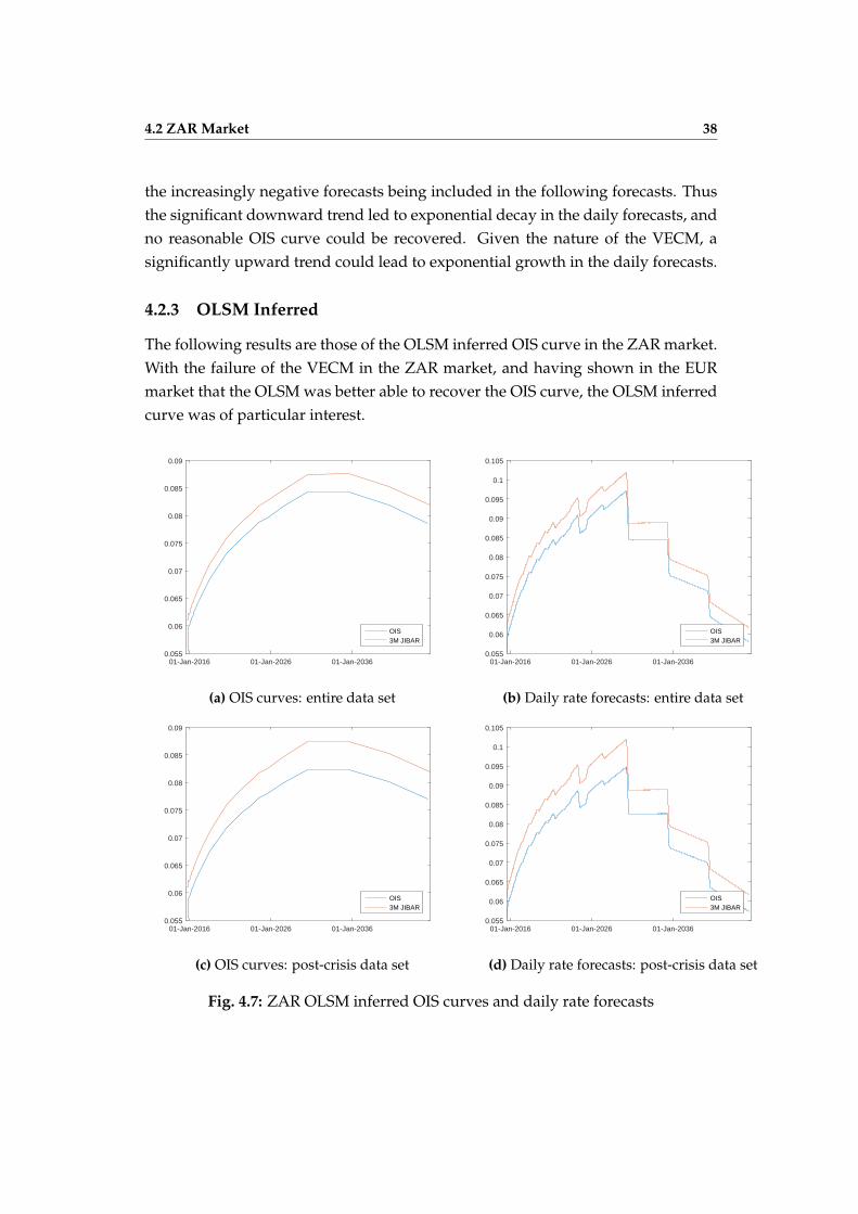
4.2.3 OLSM Inferred

The following results are those of the OLSM inferred OIS curve in the ZAR market.With the failure of the VECM in the ZAR market, and having shown in the EURmarket that the OLSM was better able to recover the OIS curve, the OLSM inferredcurve was of particular interest.

01-Jan-2016 01-Jan-2026 01-Jan-20360.055

0.06

0.065

0.07

0.075

0.08

0.085

0.09

OIS3M JIBAR


01-Jan-2016 01-Jan-2026 01-Jan-20360.055

0.06

0.065

0.07

0.075

0.08

0.085

0.09

0.095

0.1

0.105

OIS3M JIBAR


01-Jan-2016 01-Jan-2026 01-Jan-20360.055

0.06

0.065

0.07

0.075

0.08

0.085

0.09

OIS3M JIBAR


01-Jan-2016 01-Jan-2026 01-Jan-20360.055

0.06

0.065

0.07

0.075

0.08

0.085

0.09

0.095

0.1

0.105

OIS3M JIBAR


Fig. 4.7: ZAR OLSM inferred OIS curves and daily rate forecasts

4.2 ZAR Market 39

It can be seen from Figure 4.7 that the OLSM inferred what appeared to be areasonable OIS curve. Due to the simple regression structure, in which the 3MJIBAR was essentially treated as an exogenous variable, the OLSM did not sufferfrom the impact of the long term trend and autoregressive component that resultedin the failure of the VECM. As a result, the OLSM was able to infer the OIS curveunder significant upward or downward trends in historical reference rate data.

When comparing the performance of the entire and post-crisis data sets, thespread between the 3M JIBAR and inferred OIS curves was considered. It can beseen that the spread between the curves was notably greater in the post-crisis data,which was found to be the case in the EUR market. Thus, considering the EURmarket results, it was deduced that the OLSM inferred OIS curve under the entiredata set was the better estimate for the ZAR market.

Table 4.5 shows the zero curve rates for both 3M JIBAR and the inferred OIS, aswell as the basis point spread between the rates. It can be seen that the spread be-tween the rates lies around 20 bps int he short-end, widening to 30 bps and over inthe long-end. The initial spread of around 50 bps quickly to 20bps, before wideningback to 30 bps in the long-end. This change in spread level could be attributed tothe compounding of the inferred daily OIS rates used to construct the OIS curve.

4.2 ZAR Market 40

Tab. 4.5: ZAR OLSM inferred OIS against 3M JIBAR

Date 3M JIBAR (%) OIS Rate (%) Spread (bps)

16-Oct-2015 6.1107 5.5300 -58.069816-Nov-2015 6.2182 5.9709 -24.730817-Dec-2015 6.2119 6.0067 -20.512718-Jan-2016 6.2554 6.0433 -21.213116-Feb-2016 6.3036 6.0754 -22.815016-Mar-2016 6.3318 6.1075 -22.429918-Apr-2016 6.3542 6.1430 -21.123216-May-2016 6.4102 6.1712 -23.900817-Jun-2016 6.4287 6.2040 -22.467018-Jul-2016 6.4625 6.2339 -22.860417-Oct-2016 6.5571 6.3276 -22.947616-Jan-2017 6.6529 6.4182 -23.466918-Apr-2017 6.7432 6.5033 -23.981417-Jul-2017 6.8254 6.5788 -24.656416-Jul-2018 7.1194 6.8601 -25.929516-Jul-2019 7.3653 7.0958 -26.948216-Jul-2020 7.5743 7.2968 -27.740816-Jul-2021 7.7557 7.4704 -28.522218-Jul-2022 7.9008 7.6102 -29.052417-Jul-2023 8.0362 7.7437 -29.247216-Jul-2024 8.1788 7.8764 -30.241816-Jul-2025 8.2616 7.9597 -30.198116-Jul-2027 8.4718 8.1649 -30.694116-Jul-2030 8.7427 8.4199 -32.275116-Jul-2035 8.7533 8.4191 -33.421516-Jul-2040 8.5334 8.1931 -34.028518-Apr-2045 8.2027 7.8623 -34.0459

4.3 Further Discussion and Extensions 41

4.3 Further Discussion and Extensions

Based on the results of the implementation of the statistical models, further pointson the application and extension of such models were considered.

Given the form of the OLSM, it is possible to create a synthetic OIS rate bytaking the respective holdings in each of the different tenor LIBOR rates, as perthe model parameters. Such a synthetic OIS rate could be used to effect a statisticalarbitrage, by comparing the synthetic OIS rate to the realised OIS rate. Should thereexist a difference between the two, it could indicate the deviation of the OIS ratefrom a long run equilibrium relative to the different tenor LIBOR rates.

The synthetic OIS rate could be used as a statistical hedge for the OIS, as takingpositions in the longer tenored LIBOR rates would lock in the synthetic OIS ratefor a given period of time (dependent on the number of tenor LIBOR rates used inthe hedge). Furthermore, the synthetic OIS would be less volatile than the realisedOIS rate, as the synthetic volatility is a function of the the less volatile tenor LIBORrates. It is worth noting that implementing such a statistical hedge could incurhigh costs, as significant long and short positions would be required in each of thedifferent tenor LIBOR rates.

The implementation of the short-end bootstrapping procedure detailed in Clarke(2010b) is a possible extension of the implementation of the statistical models. Theassumption of flat OIS and tenor LIBOR rates out till future meeting dates could bewell suited to the application of the OLSM. As it would be expected that the OISand tenor LIBOR rates remain at similar spreads, the use of the OLSM to infer thelevel of the OIS based on the different tenor LIBOR rates should allow for the OISlevel to be reasonably well inferred. This could then be extended to the short-endbootstrapping procedure.

4.4 Chapter Summary

The implementation of statistical models and bootstrapping procedures showedthe potential application of such methods to infer the OIS curve. Key considera-tions include that of the data set used to estimate the parameters of the model, theexistence of autoregressive and trend components, and the number and tenor ofrates used in the statistical model. It was found the OLSM significantly outper-formed the VECM model in both the EUR and ZAR market. Furthermore, it wasshown that use of the entire data set over that of the post-crisis data set producedbetter OIS curve estimates. In the case of the EUR market, better estimates couldbe obtained by excluding the 12M tenor LIBOR rate, highlighting that not all tenor

4.4 Chapter Summary 42

LIBOR rates were required to recover the OIS curve.

Chapter 5

Conclusion

Research of the current market methods allowed for the OIS and different tenorLIBOR curves to be bootstrapped under such procedures. This was done in boththe EUR market, under a multi-curve framework, and the ZAR market, under asingle-curve framework. The market implied curves in the EUR market wouldserve as a baseline, allowing for the performance of the statistical models to bemeasured.

Historical reference rate data was used to test for the existence of cointegratingrelationships between OIS and LIBOR rates, in both the EUR and ZAR markets.The Johansen procedure and Engle-Granger approach were used to determine thenature of the cointegrating relationship and estimate parameters for the VECM andOLSM. It was found in general that the different tenor LIBOR and OIS rates exhib-ited strong cointegrating relationships within each of their respective markets. Inthe case of the EUR market, cointegrating relationships were still found to existwhen considering the different multivariate cases. These cointegrating relation-ships validated the use of the OLSM and VECM to model the relationship betweentenor LIBOR and OIS rates. The parameter estimates for each of the models werefound to vary when considering data sets spanning different time periods, as a re-sult of the different nature and trend of reference rates over the period. In particu-lar, the general upward or downward trend and spread between rates were foundto have greatest impact on parameter estimates. The VECM and OLSM residu-als were tested for heteroskedasticity, with all but the ZAR VECM exhibiting sucheffects. The existence of heteroskedasticity could be attributed to the nature andvolatility of the OIS rates. As these effects do not invalidate the use of the statisticalmodels, no consideration was give to alternative models.

Bootstrapping procedures were developed for both the EUR and ZAR markets,allowing the implementation of the statistical models in both a single- and multi-curve framework. The bootstrapping procedures inferred daily OIS rate forecastsfrom forward tenor LIBOR rates, allowing for both the OIS and tenor LIBOR curves

Chapter 5. Conclusion 44

to be bootstrapped whilst recovering market rates. Under implementation in thesimultaneous bootstrapping procedure (EUR market), notable differences in theperformance of the VECM and OLSM was observed. These differences could beattributed to the autoregressive and long run trend components of the VECM, andled to the failure of the VECM to capture the correct term structure of the OIS anddifferent tenor LIBOR curves. In the ZAR market, these components resulted in theexponential decay of daily OIS rate forecasts, invalidating the use of the VECM. Thetreatment of different tenor LIBOR rates as exogenous variables under the OLSMallowed for the correct term structure to be captured, with autoregressive and thelong run trend components no longer influencing results. Under the implementa-tion of the procedures, the importance of the data set was highlighted. Use of theentire data set parameters provided reasonable results, whilst the post-crisis dataset parameters failed to infer a reasonable OIS curve. This was due to differencesin the spread between reference rates across the data sets. When considering mul-tivariate cases in the EUR market, it was found that including too few LIBOR ratesproduced poor results, however inclusion of all rates was not necessary to recoverthe OIS curve effectively. The exclusion of the 12M LIBOR rate produced improvedresults over the full OLSM, highlighting that the shorter tenored LIBOR rates maybe closer related to the OIS rate. Based on the results of the implementation of thestatistical models in the bootstrapping procedures, the preferred model was foundto be that of the OLSM, with parameters estimated over the entire data set. Thus itis recommended that this model be used for the bootstrapping of the OIS curve inthe ZAR market.

Bibliography

Ametrano, F. and Bianchetti, M. (2009). Bootstrapping the illiquidity, ModellingInterest Rates: Advances for Derivatives Pricing .

Banerjee, A., Dolado, J. J., Galbraith, J. W. and Hendry, D. (1993). Co-integration,Error Correction, and the Econometric Analysis of Non-Stationary Data, Oxford Uni-versity Press.

Clarke, J. (2010a). Constructing a Non-USD Swap Discounting Curve with USDCollateral, Edu-Risk International, available at www. edurisk. ie .

Clarke, J. (2010b). Constructing the OIS Curve, Edu-Risk International, available atwww. edurisk. ie .

Clarke, J. (2010c). Swap Discounting & Pricing Using the OIS Curve, Edu-Risk In-ternational, available at www. edurisk. ie .

Dickey, D. A. and Fuller, W. A. (1979). Distribution of the Estimators for Autore-gressive Time Series with a Unit Root, Journal of the American Statistical Association74: 427–431.

Engle, R. F. (1982). Autoregressive conditional heteroscedasticity with estimates ofthe variance of United Kingdom inflation, Econometrica: Journal of the EconometricSociety pp. 987–1007.

Engle, R. F. and Granger, C. W. (1987). Co-integration and error correction: repre-sentation, estimation, and testing, Econometrica: journal of the Econometric Societypp. 251–276.

Hull, J. C. and White, A. (2013). LIBOR vs. OIS: The derivatives discountingdilemma, The Journal of Investment Management, Forthcoming .

Jakarasi, T., Labuschagne, C. C. and Mahomed, O. (2015). Estimating the SouthAfrican Overnight Indexed Swap Curve, Procedia Economics and Finance 24: 296–305.

Johansen, S. (1995). Likelihood-based inference in cointegrated vector autoregressive mod-els, Oxford University Press on Demand.

Johansen, S. and Juselius, K. (1990). Maximum likelihood estimation and inferenceon cointegrationwith applications to the demand for money, Oxford Bulletin ofEconomics and statistics 52(2): 169–210.

BIBLIOGRAPHY 46

White, R. (2012). Multiple Curve Construction, Quantitative Research, OpenGamma .

Appendix A

Boostrapping Instruments

Appendix A. Boostrapping Instruments 48

Tab. A.1: EUR OIS Market Instruments

Instrument Tenor Type

EONIA 1 day DEPEUSWE1Z 7 day SWPEUSWE2Z 14 day SWPEUSWEA 1 month SWPEUSWEB 2 month SWPEUSWEC 3 month SWPEUSWED 4 month SWPEUSWEE 5 month SWPEUSWEF 6 month SWPEUSWEG 7 month SWPEUSWEH 8 month SWPEUSWEI 9 month SWPEUSWEJ 10 month SWPEUSWEK 11 month SWPEUSWE1 12 month SWPEUSWE1F 18 month SWPEUSWE2 2 year SWPEUSWE2F 30 month SWPEUSWE3 3 year SWPEUSWE4 4 year SWPEUSWE5 5 year SWPEUSWE6 6 year SWPEUSWE7 7 year SWPEUSWE8 8 year SWPEUSWE9 9 year SWPEUSWE10 10 year SWPEUSWE11 11 year SWPEUSWE12 12 year SWPEUSWE15 15 year SWPEUSWE20 20 year SWPEUSWE25 25 year SWPEUSWE30 30 year SWPEUSWE35 35 year SWPEUSWE40 40 year SWPEUSWE50 50 year SWP

Tab. A.2: EUR 1M Market Instruments


EONIA 1 day DEPEUR001W 7 day DEPEUR001M 1 month DEPEUSWBV1 2 month SWPEUSWCV1 3 month SWPEUSWDV1 4 month SWPEUSWEV1 5 month SWPEUSWFV1 6 month SWPEUSWGV1 7 month SWPEUSWHV1 8 month SWPEUSWIV1 9 month SWPEUSWJV1 10 month SWPEUSWKV1 11 month SWPEUSW1V1 1 year SWPEUSW1CV1 15 month SWPEUSW1FV1 18 month SWPEUSW1IV1 21 month SWPEUSW2V1 2 year SWPEUSW3V1 3 year SWPEUSW4V1 4 year SWPEUSW5V1 5 year SWPEUSW6V1 6 year SWPEUSW7V1 7 year SWPEUSW8V1 8 year SWPEUSW9V1 9 year SWPEUSW10V1 10 year SWPEUSW12V1 12 year SWPEUSW15V1 15 year SWPEUSW20V1 20 year SWPEUSW25V1 25 year SWPEUSW30V1 30 year SWP




EONIA 1 day DEPEUR001W 7 day DEPEUR001M 1 month DEPEUR003M 3 month DEPEUFR0AD 4 month FRAEUFR0BE 5 month FRAEUFR0CF 6 month FRAEUFR0DG 7 month FRAEUSW1VC 1 year SWPEUSW2V3 2 year SWPEUSW3V3 3 year SWPEUSW4V3 4 year SWPEUSW5V3 5 year SWPEUSW6V3 6 year SWPEUSW7V3 7 year SWPEUSW8V3 8 year SWPEUSW9V3 9 year SWPEUSW10V3 10 year SWPEUSW11V3 11 year SWPEUSW12V3 12 year SWPEUSW15V3 15 year SWPEUSW20V3 20 year SWPEUSW25V3 25 year SWPEUSW30V3 30 year SWPEUSW35V3 35 year SWPEUSW40V3 40 year SWPEUSW50V3 50 year SWP


Inst Tenor Type

EONIA 1 day DEPEUR001W 7 day DEPEUR001M 1 month DEPEUR003M 3 month DEPEUR006M 6 month DEPEUFR0AG 7 month FRAEUFR0BH 8 month FRAEUFR0CI 9 month FRAEUFR0DJ 10 month FRAEUFR0EK 11 month FRAEUFR0F1 12 month FRAEUFR0G1A 13 month FRAEUFR0H1B 14 month FRAEUFR0I1C 15 month FRAEUFR0J1D 16 month FRAEUFR0K1E 17 month FRAEUFR011F 18 month FRAEUSA2 2 year SWPEUSA3 3 year SWPEUSA4 4 year SWPEUSA5 5 year SWPEUSA6 6 year SWPEUSA7 7 year SWPEUSA8 8 year SWPEUSA9 9 year SWPEUSA10 10 year SWPEUSA11 11 year SWPEUSA12 12 year SWPEUSA15 15 year SWPEUSA20 20 year SWPEUSA25 25 year SWPEUSA30 30 year SWPEUSA35 35 year SWPEUSA40 40 year SWPEUSA45 45 year SWPEUSA50 50 year SWP



Inst Tenor Type Spread

EONIA 1 day DEPEUR001W 7 day DEPEUR001M 1 month DEPEUR002M 2 month DEPEUR003M 3 month DEPEUR006M 6 month DEPEUR009M 9 month DEPEUR012M 12 month DEPEUSA2 2 year SWP EUBSS2EUSA3 3 year SWP EUBSS3EUSA4 4 year SWP EUBSS4EUSA5 5 year SWP EUBSS5EUSA6 6 year SWP EUBSS6EUSA7 7 year SWP EUBSS7EUSA8 8 year SWP EUBSS8EUSA9 9 year SWP EUBSS9EUSA10 10 year SWP EUBSS10EUSA12 12 year SWP EUBSS12EUSA15 15 year SWP EUBSS15EUSA20 20 year SWP EUBSS20EUSA25 25 year SWP EUBSS25EUSA30 30 year SWP EUBSS30


Tab. A.6: ZAR 3M Market Instruments


JIBA3M 3 month DEPSAFR0AD 4 month FRASAFR0BE 5 month FRASAFR0CF 6 month FRASAFR0DG 7 month FRASAFR0EH 8 month FRASAFR0FI 9 month FRASAFR0GJ 10 month FRASAFR0HK 11 month FRASAFR0I1 12 month FRASAFR011C 15 month FRASAFR1C1F 18 month FRASAFR1F1I 21 month FRASAFR1I2 24 month FRASASW3 3 year SWPSASW4 4 year SWPSASW5 5 year SWPSASW6 6 year SWPSASW7 7 year SWPSASW8 8 year SWPSASW9 9 year SWPSASW10 10 year SWPSASW12 12 year SWPSASW15 15 year SWPSASW20 20 year SWPSASW25 25 year SWPSASW30 30 year SWP

bootstrapping the ois curve in a south african bank

Documents