week 1 - gerzensee · week 1 michael rockinger ... rate and a forward rate agreement (fra) ... that...

Week 1

Michael Rockinger

HEC LausanneSwiss:Finance:Institute

February 2015

Illustrations I

Multicurve

Brousseau, Nikolaou, PillModeling Money Market Spreads: What Do We Learn about Refinancing Risk?

2

1 Introduction

Following August 2007, money market rates changed their behavior

dramatically.1 A positive wedge appeared among money market rates with the same

maturity but different floating-leg frequencies (Morini, 2009; Ametrano and

Bianchetti, 2009; Mercurio, 2010). For example, a three-month deposit rate shot up

compared with a three-month overnight index swap (OIS) rate, creating a spread that

became the main policy reference for the intensity of the financial crisis . Similarly,

a six-month deposit rate rose higher compared with alternative strategies for

borrowing money for six months, such as a combination of a three-month deposit

rate and a forward rate agreement (FRA) for three months, three months ahead (see

chart 1). In circles of policymakers, academics, and central bankers, the question of

what was driving the spreads sprang up vigorously in debates over how to tackle the

rising spreads.

!"#$%&'!""#$%&'()*+",-.(/$*"/.0-1,"2-0/3/"1"4('5$)1*$()"(6"1"*+0--&'()*+",-.(/$*"/.0-1,"1),"1"*+0--&'()*+"()"*+0--&'()*+"789"/.0-1,"

"

Note: The chart presents the evolution of the six-month EURIBOR-OIS spread and a combination of the three-month EURIBOR-OIS spread and a three-month FRA-OIS spread, three months ahead. Source:

1 rates, forward rate agreement rates, EURIBOR and EONIA rates, interest rate swaps, and forward rates.

Modeling Money Market Spreads

Usual arbitrage: short then forward= long run; no longer

holds

Lenders are willing to pay a premium

A prime bank may no longer be a prime bank in 3 month and

its financing cost would be higher

Find that central bank intervention can help reduce

refinancing risk

Filipovic, TrolleThe Term Structure of Interbank Risk, JFE

Extract various spreads between tenor x curves and OIS

ones

Explain those spreads with an affine multifactor model

The model allows for default component and non-default

component

Idea is to use information in CDS to measure default

component for bank representing prime banks (those guys

that can borrow unsecured funds)

The Term Structure of Interbank Risk

Bas

ispoi

nts

Jan06 Jan07 Jan08 Jan09 Jan10 Jan110

20

40

60

80

100

120

140

160

180

200

Figure 1: Money market and swap market spreads

The figures shows time-series of the spread between 3M LIBOR and the 3M OIS rate (solid line) and the spread

between the rate on a 5Y interest rate swap indexed to 3M LIBOR and the 5Y OIS rate (dotted line). Note

that the 3M LIBOR-OIS spread reached a maximum 366 basis points on October 10, 2008. The vertical dotted

lines mark the beginning of the financial crisis on August 9, 2007, the sale of Bear Stearns to J.P. Morgan on

March 16, 2008, the Lehman Brothers bankruptcy filing on September 15, 2008, and the downgrade of Greece’s

debt to non-investment grade status by Standard and Poor’s on April 27, 2010. Both time series consists of

1313 daily observations from January 02, 2006 to January 12, 2011.

51

Maturity

3M 6M 1Y 2Y 3Y 4Y 5Y 7Y 10Y

Panel A: USD market

OIS 1.17(1.48)

1.17(1.43)

1.26(1.35)

1.63(1.21)

2.06(1.12)

2.42(1.03)

2.72(0.96)

3.17(0.55)

†

SPREAD3M 58.7(57.5)

51.2(34.6)

43.8(23.2)

39.0(17.2)

35.4(14.0)

32.5(11.9)

28.7(8.2)

†

SPREAD6M 79.1(57.4)

70.0(42.7)

58.0(28.2)

50.8(20.8)

45.8(16.9)

41.9(14.2)

38.1(7.7)

†

CDSTrMean 67.8(46.5)

70.2(44.9)

78.7(41.2)

85.3(37.9)

93.4(37.0)

99.1(35.9)

102.1(34.5)

104.8(33.3)

CDSLIQ1 61.1(41.9)

63.2(40.4)

70.9(37.1)

76.8(34.1)

84.1(33.3)

89.2(32.3)

91.9(31.0)

94.3(30.0)

CDSLIQ2 78.7(55.1)

82.9(53.4)

91.2(48.4)

98.8(45.0)

106.2(43.0)

113.1(42.0)

114.6(40.7)

116.6(39.2)

Panel B: EUR market

OIS 1.91(1.67)

1.93(1.65)

2.00(1.58)

2.21(1.38)

2.45(1.23)

2.67(1.13)

2.85(1.02)

3.14(0.87)

3.44(0.74)

SPREAD3M 58.7(35.6)

49.6(21.7)

43.0(15.2)

39.6(12.2)

36.0(11.3)

34.3(10.0)

32.0(8.6)

29.9(7.4)

SPREAD6M 73.5(36.2)

66.3(24.4)

55.9(16.1)

50.6(13.0)

45.7(12.9)

43.1(11.8)

39.6(10.5)

36.2(9.2)

CDSMedian 70.5(43.0)

72.9(40.5)

81.3(37.7)

88.6(35.9)

95.8(35.2)

102.3(34.8)

104.8(34.4)

107.3(33.9)

CDSLIQ1 63.4(38.7)

65.6(36.4)

73.2(33.9)

79.7(32.3)

86.2(31.7)

92.1(31.3)

94.3(31.0)

96.6(30.5)

CDSLIQ2 64.9(39.3)

67.8(38.6)

76.1(36.2)

83.8(35.2)

90.9(35.0)

97.4(35.3)

99.6(34.9)

102.1(34.5)

CDSiT raxx 104.0(39.0)

109.0(37.2)

Notes: The table shows means and, in parentheses, standard deviations. SPREAD3M denotes the di!erencebetween the fixed rates on an IRS indexed to 3M LIBOR/EURIBOR and an OIS with the same maturity.SPREAD6M denotes the di!erence between the fixed rates on an IRS indexed to 6M LIBOR/EURIBOR andan OIS with the same maturity. CDSTrMean and CDSMedian are the CDS spread term structures for therepresentative LIBOR and EURIBOR panel banks, respectively. CDSLIQ1, and CDSLIQ2 are the CDS spreadterm structures corrected for possible liquidity e!ects as described in the main text. CDSiTraxx is the iTraxxSenior Financials CDS index. OIS rates are measured in percentages, while interest rate spreads and CDSspreads are measured in basis points. Each time series consists of 895 daily observations from August 09, 2007to January 12, 2011, except those marked with † which consist of 643 daily observations from July 28, 2008 toJanuary 12, 2011.

Table 1: Summary statistics of data

Bank Currency Mean CDS Std CDS Balance Liquidity Start date

Bank of America USD 136 62 2230 203 09-Aug-2007

Bank of Tokyo Mitsubishi USD 71 28 1619 17 09-Aug-2007

Barclays EUR 111 46 2227 117 09-Aug-2007

Citigroup USD 201 122 1857 155 09-Aug-2007

Credit Suisse EUR 108 40 997 71 06-May-2008

Deutsche Bank EUR 95 32 2151 159 09-Aug-2007

HSBC EUR 75 29 2364 38 09-Aug-2007

J. P. Morgan Chase USD 92 36 2032 174 09-Aug-2007

Lloyds TSB EUR 122 58 925 58 09-Aug-2007

Rabobank EUR 77 39 871 —— 09-Aug-2007

Royal Bank of Canada USD 75 36 606 —— 09-Aug-2007

Societe Generale EUR 93 34 1467 66 09-Aug-2007

Norinchukin Bank USD 85 41 630 2 09-Aug-2007

RBS EUR 134 53 2739 117 09-Aug-2007

UBS EUR 120 62 1296 81 09-Aug-2007

WestLB EUR 118 41 347 16 09-Aug-2007

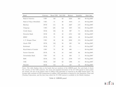
Notes: The table displays data on the banks that are members of the LIBOR panel. For each bank, it showsthe currency of the CDS contracts, the mean and standard deviation of the 5Y CDS spread in basis pointsper annum, the size of the balance sheet in billion USD equivalent as reported in the 2009 annual report, theaverage daily notional of CDS transactions in million USD equivalent as reported by the Depository Trust andClearing Corporation, and the date from which the 5Y CDS contract is available in the Markit database.

Table 2: LIBOR panel

Model

Relatively complicated model

(Miracle that they could estimate it)

models interest rates rt

involves default intensities λt of firms

involves a non-default component ξt

Algebra for various components is non-trivial

Maturity

3M 6M 1Y 2Y 3Y 4Y 5Y 7Y 10Y

Panel A1: SPREAD3M , USD market

Default 28.1(26.8)

25.2(17.2)

24.0(12.5)

23.8(10.7)

23.9(9.8)

24.1(9.2)

28.6(5.8)

†

Non-default 33.4(45.2)

20.4(27.3)

10.6(14.1)

7.2(9.5)

5.5(7.3)

4.5(6.0)

1.8(3.5)

†

Panel A2: SPREAD6M , USD market

Default 45.9(39.7)

43.1(30.1)

40.9(21.8)

40.5(18.5)

40.7(16.8)

41.0(15.7)

48.6(10.0)

†


29.6(40.5)

15.6(21.2)

10.6(14.3)

8.1(10.9)

6.7(8.9)

2.9(5.4)

†

Panel B1: SPREAD3M , EUR market

Default 28.6(23.1)

24.2(13.7)

22.5(10.0)

22.1(8.8)

22.1(8.2)

22.2(7.9)

22.7(7.5)

23.4(7.2)


21.9(22.8)

11.7(12.0)

8.0(8.2)

6.2(6.3)

5.1(5.1)

3.9(3.8)

3.0(2.8)

Panel B2: SPREAD6M , EUR market

Default 46.7(34.0)

42.4(24.7)

39.3(17.9)

38.5(15.6)

38.5(14.5)

38.7(13.8)

39.4(13.1)

40.8(12.5)


31.0(31.2)

17.3(17.1)

11.9(11.7)

9.2(8.9)

7.6(7.3)

5.8(5.4)

4.5(4.0)

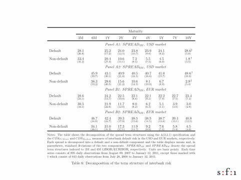
Notes: The table shows the decomposition of the spread term structures using the A(2,2,1) specification andthe CDSTrMean and CDSMedian measures of interbank default risk in the USD and EUR markets, respectively.Each spread is decomposed into a default and a non-default component and the table displays means and, inparentheses, standard deviations of the two components. SPREAD3M and SPREAD6M denote the spreadterm structures indexed to 3M and 6M LIBOR/EURIBOR, respectively. Units are basis points. Each timeseries consists of 895 daily observations from August 09, 2007 to January 12, 2011, except those marked with† which consist of 643 daily observations from July 28, 2008 to January 12, 2011.

Table 6: Decomposition of the term structure of interbank risk

Panel A: 3M spread Panel B: 6M spread

Panel C: 5Y(3M) spread Panel D: 5Y(6M) spread

Jan08 Jan09 Jan10 Jan11Jan08 Jan09 Jan10 Jan11


0

20

40

60

80

100

0

20

40

60

80

100

0

100

200

300

400

0

100

200

300

400

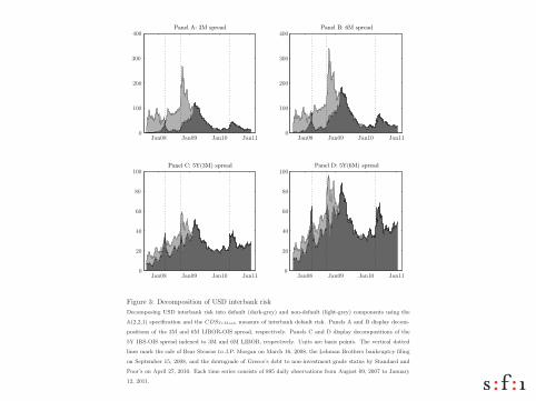
Figure 3: Decomposition of USD interbank risk

Decomposing USD interbank risk into default (dark-grey) and non-default (light-grey) components using the

A(2,2,1) specification and the CDSTrMean measure of interbank default risk. Panels A and B display decom-

positions of the 3M and 6M LIBOR-OIS spread, respectively. Panels C and D display decompositions of the

5Y IRS-OIS spread indexed to 3M and 6M LIBOR, respectively. Units are basis points. The vertical dotted

lines mark the sale of Bear Stearns to J.P. Morgan on March 16, 2008, the Lehman Brothers bankruptcy filing

on September 15, 2008, and the downgrade of Greece’s debt to non-investment grade status by Standard and

Poor’s on April 27, 2010. Each time series consists of 895 daily observations from August 09, 2007 to January

12, 2011.

53

Panel A: 3M spread Panel B: 6M spread

Panel C: 5Y(3M) spread Panel D: 5Y(6M) spread



0

20

40

60

80

100

0

20

40

60

80

100

0

50

100

150

200

250

0

50

100

150

200

250

Figure 4: Decomposition of EUR interbank risk

Decomposing EUR interbank risk into default (dark-grey) and non-default (light-grey) components using the

A(2,2,1) specification and the CDSMedian measure of interbank default risk. Panels A and B display decompo-

sitions of the 3M and 6M EURIBOR-OIS spread, respectively. Panels C and D display decompositions of the

5Y IRS-OIS spread indexed to 3M and 6M EURIBOR, respectively. Units are basis points. The vertical dotted

lines mark the sale of Bear Stearns to J.P. Morgan on March 16, 2008, the Lehman Brothers bankruptcy filing

on September 15, 2008, and the downgrade of Greece’s debt to non-investment grade status by Standard and

Poor’s on April 27, 2010. Each time series consists of 895 daily observations from August 09, 2007 to January

12, 2011.

54

Explaining the “Non-Default” Component

Use funding- and market- liquidity measures

MBS-Treasury

repo

Fails OIS-Tbill HPW noise adj. R2

Panel A: USD market

0.042(3.635)

!!! 0.289

15.316(6.366)

!!! 0.296

0.019(1.910)

! 0.071

0.934(7.291)

!!! 0.616

0.036(1.942)

! 7.653(1.673)

! 0.395

0.006(0.678)

0.910(6.864)

!!! 0.622

0.014(1.111)

3.633(0.790)

!0.003("0.347)

0.772(5.407)

!!! 0.654

Panel B: EUR market

0.015(2.255)

!! 0.162

5.014(3.467)

!!! 0.137

0.002(0.786)

0.004

0.367(4.707)

!!! 0.479

0.014(1.387)

1.979(0.981)

0.208

!0.004("1.138)

0.381(4.899)

!!! 0.489

0.008(1.350)

0.850(0.494)

!0.005("1.265)

0.338(4.341)

!!! 0.528

Notes: The table reports results from regressing !(t) inferred from the A(2,2,1) specification on two fundingliquidity measures (the 3M MBS-Treasury repo rate spread and the weekly sum of the notional amount ofTreasury settlement fails (average of failure to deliver and failure to receive) reported by primary dealers) andtwo market liquidity measures (the 3M OIS-Tbill spread and the Hu, Pan, and Wang (2010) noise measure).Each of the liquidity time series are orthogonalized with respect to the first two principal components of theCDS term structure. The settlement fails data is in USD trillions, while the rest are in basis points. Ineach panel, the regressions are run with daily data, except the second, fifth, and seventh regressions involvingTreasury settlement fails, which are run with weekly data (summing up the daily observations over the week).T -statistics, corrected for heteroscedasticity and serial correlation up to 22 lags in the daily regressions (4 lags inthe weekly regressions) using the method of Newey and West (1987), are in parentheses. !, !!, and ! ! ! denotesignificance at the 10%, 5%, and 1% levels, respectively. Each time series consists of 600 daily observations (or125 weekly observations) from August 09, 2007 to December 31, 2009,

Table 7: The non-default component and liquidity

Illustrations II

Illustrations on Risk Neutral Densities

First generation: just extracting the densities

Second generation: go to real world densities

Recent implementations

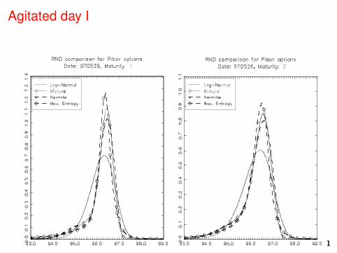
Coutant, Jondeau, RockyReading PIBOR futures options smiles: The 1997 snap election

!"#" $%&'()*+ #,' -'()%. /(%0 1'2(3"(4 56 7889 #% :3;4 5<6 7889 %* =>?@A/3#3('BC%-#)%*B "B D';; "B %* #,' 3*.'(;4)*+ /3#3('B $%*#("$# ,"B 2''* E)*.;4-(%&).'. 24 FGH>1I J

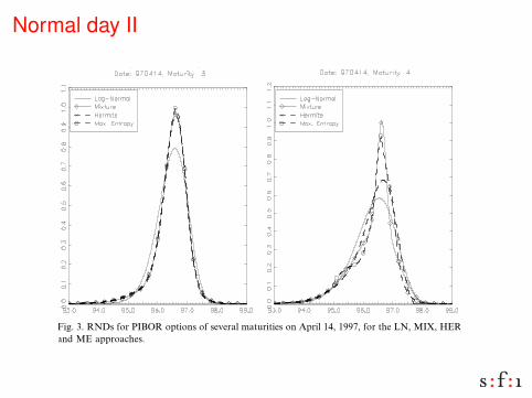
1)+BI 7 "*. K .)B-;"4 &%;"#);)#)'B "+")*B# B#()E' -()$'B /%( #D% B';'$#'. ."#'BI 9

L402%;B %* #,' &"()%3B $3(&'B $%(('B-%*. #% ."#" -(%&).'. 24 FGH>1IM,'*'&'( B402%;B "(' %* " B#(")+,# ;)*'6 #,'4 $"* 2' "BB30'. #% ,"&' 2''*%2#")*'. D)#, " ;)*'"( )*#'(-%;"#)%*I >* %#,'( D%(.B6 %*;4 B402%;B D,'(' #,';)*' ,"B " E)*E "(' ;)E';4 #% $%(('B-%*. #% "$#3"; )*/%(0"#)%*I M' ";B% *%#)$'#,"# FGH>1 .%'B *%# B4B#'0"#)$";;4 -(%&).' )*#'(-%;"#'. &%;"#);)#)'BI 1%( )*CB#"*$'6 %* G-(); 7N6 7889 /%( #,' =>?@A %-#)%* D)#, ,)+,'B# 0"#3()#46 " O3%#'D"B ('-%(#'. /%( #,' 8JI< "*. #,' 8JIK B#()E' 23# *%# /%( #,' 8JI7 B#()E'I H,'B'%2B'(&"#)%*B B3++'B# #,"# #,' 0'#,%.B 3B'. #% 'P#("$# )*/%(0"#)%* B,%3;. ";C;%D /%( -%BB)2;' %-#)%*B 0)B-()$)*+6 "*. ";B% #,"# %*' B,%3;. $%*B).'( Q;#'(B2'/%(' 3B)*+ #,)B ("D ."#"I

1)+I 7I L0);'B /%( =>?@A %-#)%*B %/ B'&'("; 0"#3()#)'B %* G-(); 7N6 7889I H,' B402%;B !6 "6 #6"*. ! $%(('B-%*. #% %-#)%*B D)#, J56 7RN6 KNR6 "*. 55J ."4B #% 0"#3()#4I

J >*/%(0"#)%* %* ,%D #,' FGH>1 %-'("#'B $"* 2' /%3*. 3*.'( #,' D'2C-"+'S ,##-STTDDDI0"#)/I/(TI

9 >* %(.'( #% B)0-;)/4 #,' Q+3('B6 #,' 'P#("-%;"#)%*B "# $%*B#"*# &%;"#);)#4 ;'&'; #% #,' ;'/# "*. #%#,' ()+,# %/ #,' B0);' ,"&' ";('".4 2''* .)B$"(.'.I

78JK !" #$%&'(& )& '*" + ,$%-('* $. /'(01(2 3 41('(5) 67 8699:; :<7=>:<?=

Pibor futures

!"#$# %&'(#$ )*$+ "),# )- #.+-+/0. 0/1*0.)20+-3 4"#- 5# .+-$06#( 789:;+120+-$ +< ) $)/# /)2'(02= 0- >0&$3 ? +( @A 5# -+20.# 2")2 +120+-$ 502" 60B#(#-2$2(0C#$ "),# 60B#(#-2 0/1*0#6 ,+*)20*020#$3 !"0$ <#)2'(# 0$ 1(#.0$#*= 2"# !"#$!%&'$()3 4# )*$+ -+20.# 2"# ,#(20.)* $"0<2 +< $/0*#$ )$ /)2'(020#$ .")-&#3 !"0$.+((#$1+-6$ 2+ 2"# <#)2'(# *)D#*#6 0- 2"# *02#()2'(# )$ ) #)*' &#*+,#+*) !-.!(/#$($#$)&3 >+( E1(0* ?FA ?GGHA ) 6)2# +-# 5##C D#<+(# 2"# +I.0)* )--+'-.#/#-2+< 2"# $-)1 #*#.20+-A "0&"#( /)2'(020#$ )(# )$$+.0)2#6 502" "0&"#( ,+*)20*02=3 J 4#50** (#<#( 2+ E1(0* ?F )$ 2"# %!*'/( 6)2#3 4"#- 5# 2)C# K)= @LA 2"# 6)= )<2#( 2"#%($2 #*#.20+- (+'-6A 5# -+20.# 2"# (#,#($)* +< 2"# 2#(/ $2('.2'(# +< ,+*)20*02=A/#)-0-& 2")2 +1#()2+($ ")6 *+2$ +< '-.#(2)0-2= .+-.#(-0-& 2"# $"+(2 ('-3

!" #$% &%'%()* +(),%-.(/

0121 34) 5*/,)6 7/#/*)86 /%9 :+&$)(/ ;)%,4'/*8 '!9)(

K)-= 0-2#(#$2M()2# /+6#*$ "),# D##- 1(+1+$#6 0- 2"# *02#()2'(#3 8- ) %($2.)2#&+(= +< /+6#*$A 2"# 0-2#(#$2M()2# .'(,# )-6 2"# 60$.+'-2 <).2+( )(#

>0&3 @3 N/0*#$ <+( 789:; +120+-$ +< $#,#()* /)2'(020#$ +- K)= @LA ?GGH3 !"# $=/D+*$ !A "A #A )-6! .+((#$1+-6 2+ +120+-$ 502" OLA ?FHA @PJA )-6 P@G 6)=$ 2+ /)2'(02=3

J E$ $"+5- *)2#(A +- 2"0$ 6)2# /)(C#2 /)C#($ 606 -+2 =#2 )-20.01)2# 2"# #*#.20+-3

<1 =!+#/%# )# /(1 > ?!+*%/( !- 5/%8$%@ A B$%/%,) CD ECFF2G 2HDIJ2HKI ?GLP

Normal day I

!"#$% &'()&*+ ,-&.-,/ (01&230 ()4,5 6* ,-,*( &7 31,8( '&.)()98. )4'&1(8*9,&9921+ )* &21 /8(8:8+,; *84,.< (0, =>>? +*8' ,.,9()&*5 @&1 (0, AB; C,44)..D=>>EF )*-,+()38(,/ )7 (0, &'()&*+ 481G,( 7&1,98+( 8* ,.,9()&* &2(9&4,5

@)35 H5 %IJ+ 7&1 !"#$% &'()&*+ &7 +,-,18. 48(21)(),+ &* 6'1). =K; =>>?; 7&1 (0, LI; M"N; OP%;8*/ MP 8''1&890,+5

!" #$%&'(& )& '*" + ,$%-('* $. /'(01(2 3 41('(5) 67 8699:; :<7=>:<?= =>?Q

Normal day II

!"#$% &'()&*+ ,-&.-,/ (01&230 ()4,5 6* ,-,*( &7 31,8( '&.)()98. )4'&1(8*9,&9921+ )* &21 /8(8:8+,; *84,.< (0, =>>? +*8' ,.,9()&*5 @&1 (0, AB; C,44)..D=>>EF )*-,+()38(,/ )7 (0, &'()&*+ 481G,( 7&1,98+( 8* ,.,9()&* &2(9&4,5

@)35 H5 %IJ+ 7&1 !"#$% &'()&*+ &7 +,-,18. 48(21)(),+ &* 6'1). =K; =>>?; 7&1 (0, LI; M"N; OP%;8*/ MP 8''1&890,+5

!" #$%&'(& )& '*" + ,$%-('* $. /'(01(2 3 41('(5) 67 8699:; :<7=>:<?= =>?Q

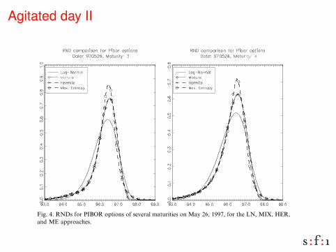
Agitated day I

!" "#$% %"&'() *( (+,#&%$-( "#&" *( &.( $/"(.,.("$/' +0+(/"% 1(.$2(1 3.0+"#( 456% &% $3 "#(7 *(.( 08"&$/(1 $/ "#( &9":&; *0.;1< =#$% $% 8&%(1 0/ "#(.(+&.> 87 4:8$/%"($/ ?@AABC "#&"D EE! ! ! 1(%,$"( *&./$/'% "0 "#( 90/".&.7) *(

F$'< B< 456% 30. GHIJ4 0,"$0/% 03 %(2(.&; +&":.$"$(% 0/ K&7 LM) @AAN) 30. "#( O5) KHP) QR4)&/1 KR &,,.0&9#(%<

@ANM !" #$%&'(& )& '*" + ,$%-('* $. /'(01(2 3 41('(5) 67 8699:; :<7=>:<?=

Agitated day II

!" "#$% %"&'() *( (+,#&%$-( "#&" *( &.( $/"(.,.("$/' +0+(/"% 1(.$2(1 3.0+"#( 456% &% $3 "#(7 *(.( 08"&$/(1 $/ "#( &9":&; *0.;1< =#$% $% 8&%(1 0/ "#(.(+&.> 87 4:8$/%"($/ ?@AABC "#&"D EE! ! ! 1(%,$"( *&./$/'% "0 "#( 90/".&.7) *(

F$'< B< 456% 30. GHIJ4 0,"$0/% 03 %(2(.&; +&":.$"$(% 0/ K&7 LM) @AAN) 30. "#( O5) KHP) QR4)&/1 KR &,,.0&9#(%<

@ANM !" #$%&'(& )& '*" + ,$%-('* $. /'(01(2 3 41('(5) 67 8699:; :<7=>:<?=

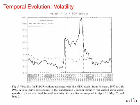
Temporal Evolution: Volatility

!"# $%&'()"*+, &%--.&/ " 0.%12 &(3(+"0(', */'4//# '2/ 0(&56#/%'0"+ -0.*"*(+('(/&(3-+(/7 (# .-'(.# -0(!/& "#7 &%*$/!'(8/ */+(/9&::; <%*(#&'/(# $%&'()/& '2(& 4('2 "#%3/0(!"+ /="3-+/; >.0 '2/ )1%0/& -0/&/#'/7 */+.4 '2(& (3-+(/& '2"' "#,#%3*/0 &2.%+7 */ !.#&(7/0/7 "& "# "--0.=(3"'(.# .9 '2/ "!'%"+ .#/; ?2%&@!2"#1/& (# '2/ #%3*/0& "0/ 3.0/ (#9.03"'(8/ '2"# '2/ "!'%"+ +/8/+&;

>(1; A &2.4& %& 2.4 %#!/0'"(#', .9 3"05/' .-/0"'.0& /8.+8/7 '20.%12 '(3/;B/ #.'(!/ '2/ 0/+"'(8/ !"+3 (# '2/ 3"05/' */9.0/ C-0(+ DE; ?2/# 8.+"'(+(', *%(+7&%- (# '2/ 4//5 */9.0/ '2/ .F!("+ "##.%#!/3/#' .9 '2/ &#"- /+/!'(.# .!!%00/7;C9'/0 '2/ .F!("+ "##.%#!/3/#' .# C-0(+ GD@ %#!/0'"(#', 0/3"(#/7 !.#&'"#';?2/# !"3/ '2/ &%0-0(&/ .# H", GI '2"' '2/ 1.8/0#3/#' 3(12' !2"#1/; ?2(&%#!/0'"(#', 0.&/ /8/# 9%0'2/0 "& -.++& 0/8/"+/7 '2/ -.&&(*(+(', .9 " &.!("+(&'8(!'.0,; J# K%#/ G@ (' */!"3/ !+/"0 '2"' '2/ &.!("+(&'& 2"7 4.#; C& '2/, 2/+70/"&&%0(#1 '"+5& "*.%' '2/(0 &'"#!/ .# '2/ L%0.-/"# H.#/'"0, M#(.# "#7 '2/(01/#/0"+ /!.#.3(! -.+(!,@ 3"05/'& !"+3/7 7.4# 0"'2/0 N%(!5+,;

O# >(1; I@ 4/ '%0# '. P'2/ #/1"'(8/ .9Q '2/ -0(!/ .9 &5/4#/&& 42(!2 9%0'2/0(#7(!"'/& '2"' .-/0"'.0& /=-/!'/7 7(0/!'(.#"+ 3.8/& .9 (#'/0/&' 0"'/&; R+/"0+,'2(& 3/"&%0/ 2"& 10/"'/0 8"0("*(+(', '2"# 8.+"'(+(',; C9'/0 '2/ .F!("+ "#6#.%#!/3/#'@ "# (#!0/"&/ (# '2/ &2.0'6'/03 0"'/ */!"3/ 3.0/ +(5/+,; S%' (#6'/0/&'(#1+,@ /8/# "9'/0 '2/ /+/!'(.# "#7 '2/ &2"0- 7/!0/"&/ (# 8.+"'(+(',@ '2/ -0(!/

>(1; A; T.+"'(+(', 9.0 UOSJ< .-'(.#& /&'(3"'/7 4('2 '2/ VL< 3.7/+@ 90.3 >/*0%"0, DWWX '. K%+,DWWX; C &.+(7 !%08/ !.00/&-.#7& '. '2/ &'"#7"07(Y/7 Z63.#'2 3"'%0(',@ '2/ 7"&2/7 !%08/ !.00/6&-.#7& '. '2/ &'"#7"07(Y/7 W63.#'2 3"'%0(',; T/0'(!"+ +(#/& !.00/&-.#7 '. C-0(+ GD@ H", GI@ "#7K%#/ G;

!" #$%&'(& )& '*" + ,$%-('* $. /'(01(2 3 41('(5) 67 8699:; :<7=>:<?= DWXX

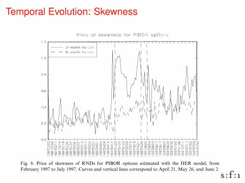
Temporal Evolution: Skewness

!" #$%&'%## (%)*+'%, (*-.%( .+/.0 +',+1*-+'/ %23%1-*-+!'# !" ,+(%1-+!'*4 )!5%#!" +'-%(%#- (*-%#6

7' 8+/6 90 &% +'5%#-+/*-% -.% %5!4:-+!' -.(!:/. -+)% !" -.% 3(+1% !" $:(-!#+#6;!)3*(+#!' &+-. 5!4*-+4+-<0 ,+#34*<%, +' 8+/6 =0 #.!&# -.*- -.%(% +# * $+', !"-(*,%!> ?%-&%%' $:(-!#+# *', 5!4*-+4+-<6 @*-%# ,+#-*'- "(!) -.% %4%1-+!' 3%(+!,.*, 4!&%( 5!4*-+4+-< ?:- .+/.%( $:(-!#+# *', 5+1% 5%(#* ,:(+'/ -.% %4%1-+!' 3%A(+!,6 B4#!0 -.% -(%', -!&*(,# .+/.%( #$%&'%## *"-%( -.% %4%1-+!'# (%5%*4# -.*-:',%( -.% '%& /!5%(')%'-0 -(*,%(# &%(% &!((+%, *?!:- 5*(+*-+!'# -!&*(,#*?'!()*4 4%5%4# !" +'-%(%#- (*-%#6 @:(+'/ -.% %4%1-+!'0 /4!?*4 :'1%(-*+'-< +'A1(%*#%, *', ,%1(%*#%, *"-%(6 C.% .+/.%( 4%5%4 !" #$%&'%## -!&*(,# -.% %', !"!:( #*)34% #://%#-# -.*-0 %5%' ?< -.% %', !" D:4< EFF90 -.% '%& /!5%(')%'-&*# :'*?4% -! ,+##!45% *44 "%*(#6

7- +# 3!##+?4% -! *'*4<G% -.+# +'"!()*-+!' +' *' *4-%('*-+5% )*''%( ?< 1!'A#+,%(+'/ 1!'H,%'1% +'-%(5*4# 1!)3:-%, &+-. IJ@#6 K%- !" *', !# ?% -.% =A *',F=A3%(1%'-+4%# !" * IJ@6 L% ,%H'% * !# ! !" *# !"#$%&'( )(*+!'+$,#- L% *4#!!?-*+' 3%(1%'-*/% ,%5+*-+!'# &+-.

!+'" " EMM$!"

!! E

"! !#:3 " EMM

!#$

!! E

"! I*'/% " EMM

!# ! !"$

! ""

N%(1%'-*/% ,%5+*-+!'# *(% (%4*-+5% -! -.% "!(&*(, 3(+1% *', *(% +',+1*-+5% !" -.%#+,% -!&*(,# &.+1. -.% IJ@ -%',#6

8+/6 O6 N(+1% !" #$%&'%## !" IJ@# "!( N7PQI !3-+!'# %#-+)*-%, &+-. -.% RSI )!,%40 "(!)8%?(:*(< EFF9 -! D:4< EFF96 ;:(5%# *', 5%(-+1*4 4+'%# 1!((%#3!', -! B3(+4 TE0 U*< TO0 *', D:'% T6

EF9V .- /$&'!,' (' !%- 0 1$&2,!% $3 4!,5+,6 7 8+,!,9( :; <:==>? >@;AB>@CA

Temporal Evolution: Kurtosis

!"#$% &# '(#)*##+' (, -+).($, /01% .2+ &3&("&4("(.5 $6 $7.($,# 8(.2 #+3+9&":&.*9(.(+# &""$8# .2+ )$,#.9*).($, $6 #.&,'&9'(;+' $7.($,#% (0+0% $7.($,# 8(.2 &<=+' .(:+ .$ :&.*9(.50 >+ 6$)*# ,$8 $, $7.($,# &94(.9&9("5 #.&,'&9'(;+' 6$9 /:$,.2# ?@A '&5#B &,' @ :$,.2# ?C1A '&5#B0 D&4"+ / '(#7"&5# )$,<'+,)+ (,E.+93&"# &# 7+9)+,.&F+ '+3(&.($,# &,' &# &4#$"*.+ '+3(&.($,#0 G(F#0 H &,' @'(#7"&5 '&("5 )$,<'+,)+ (,.+93&"#0 D$ :&I+ 9+#*".# &# +&#5 .$ (,.+979+. &#7$##(4"+% 8+ .9&,#6$9: .2+ JAA! ! K*$.+ (,.$ & 6$98&9' 9&.+ !0

G$9 .2+ ,$9:&" '&.+% 8+ <,' .2&. 6$9 .2+ @A '&5# .$ )$:+% $7+9&.$9# 4+E"(+3+' .2&. 8(.2 & @AL 79$4&4("(.5% (,.+9+#. 9&.+# 8$*"' ,$. F$ *,'+9 /0JL ,$9&4$3+ /0@L0 D2(# 9&,F+ (,)9+&#+# #*4#.&,.(&""5 6$9 .2+ @E:$,.2 #.&,'&9'(;+'$7.($,0

!# ,+8# 2(. .2+ :&9I+. 45 !79(" CJ% .2+ 8('+,(,F $6 .2+ )$,<'+,)+ (,.+93&"##*FF+#.# 6+&9# $6 "&9F+ :$3+:+,.# $6 9&.+#0 D2+#+ 6+&9# 8+9+ .2+ F9+&.+#. &6.+9.2+ <9#. 9$*,' $6 +"+).($,#0 M,+ 8++I &6.+9 .2+ #+)$,' 9$*,'% *,)+9.&(,.5 2&''+)9+&#+' 4*. 8&# #.("" 2(F20

G(F0 H F(3+# & :$9+ (,.*(.(3+ 7().*9+ $6 .2(# +3$"*.($,0 >+ ,$.()+ .2&.$7+9&.$9# 7*. & "$8+9 4$*,' $, 9&.+# 9&,F(,F 4+.8++, C0HL &,' /0JL0 N3+,.2$*F2 .2+ 6$98&9' 9&.+ '$+# ,$. :$3+ 3+95 :*)2% 8+ #++ 2*F+ 3&9(&.($,# (,.2+ *77+9 4$*,'0 D2(# (# #*FF+#.(3+ $6 6+&9# $6 &, (,)9+&#+ (, (,.+9+#. 9&.+#0!6.+9 .2+ +"+).($,#% .2+ *77+9 4$*,' '+)9+&#+#% 2$8+3+9 (. 9+:&(,# &. & 2(F2

G(F0 10 O9()+ $6 I*9.$#(# $6 PQR# 6$9 OSTMP $7.($,# &# +#.(:&.+' 45 .2+ UNP &779$&)2%69$: G+49*&95 J@@1 .$ V*"5 J@@10 W*93+# &,' 3+9.()&" "(,+# )$99+#7$,' .$ !79(" CJ% X&5 CY% &,'V*,+ C0

"# $%&'()' *' (+# , -%&.)(+ %/ 0()12)3 4 !2)()5* 67 8699:; :<7=>:<?= J@1@

Temporal Evolution: Risk Neutral Confidence Intervals

!"# !$%&'!'()%* +#),"-%$. *(/0)($-%* &'1!$'+2!'()3 45#)!2%**67 8# 1#!!*#& 9($%) %::$(;'-%!'() +%1#& () <#$-'!# :(*6)(-'%*1 &#5#*(:#& ($'/')%**6 +6=%&%) %)& ='*)# >?@@AB3 C"'1 -#!"(& 6'#*&1 %,,2$%!# #1!'-%!#1 %)& '1 %+*#!( &#%* 8'!" 1(-#8"%! &'$!6 &%!%3 D! '1 )2-#$',%**6 9%1! %)& 1!%+*#3 E*1(7 !"'1-#!"(& ,%) +# 21#& !( (+!%') 1!%)&%$&'F#& (:!'()17 '3#37 8'!" % G;#& !'-# !'**-%!2$'!63

C"#) 8# %::*'#& !"'1 -#!"(& !( &%!% $%)/')/ 9$(- H#+$2%$6 I7 !( J2*6 IK7?@@L3 H($ !"# (:!'()1 %! "%)&7 8# 9(2)& !"%! !"# -%$.#! %)!',':%!#& %) '-0:($!%)! #5#)! +#9($# !"# (M,'%* %))(2),#-#)! (,,2$$#&3 E1 :(**1 ,()G$-7 %:(11'+*# ,"%)/# (9 /(5#$)-#)! +#9($# !"# G$1! #*#,!($%* $(2)& '),$#%1#& 2)0,#$!%')!63 E9!#$ !"# 1#,()& $(2)& (9 !"# #*#,!'()17 #5#) !"(2/" 2),#$!%')!6%+(2! !"# 92!2$# &#,$#%1#&7 9#%$1 (9 ')!#$#1! $%!# '),$#%1#1 :#$1'1!#&3 N)# $%0!'()%*# '1 !"%! !"#$# #;'1! 1#5#$%* *#5#*1 (9 2),#$!%')!63 E! % G$1! *#5#* !"#$# '1 !"#2),#$!%')!6 %+(2! 8"'," :(*'!',%* :%$!6 '1 /(')/ !( 8') %)& %! %) (!"#$ *#5#*!"#$# '1 !"# :$(/$%- !"%! !"# :%$!'#1 :*%) !( '-:*#-#)!3 O'/"! %9!#$ !"# #*#,0!'()1 !"# 2),#$!%')!6 ,(),#$)')/ !"# :(*'!',%* :%$!6 &'-')'1"#& +2! !"#$# $#0-%')#& !"# 2),#$!%')!6 %+(2! !"# 92!2$# :(*'!',%* :$(/$%-3 P6 !"# #)& (9 J2*6?@@L7 8# 9(2)& !"%! !"# )#8 /(5#$)-#)! "%& )(! 6#! $#%112$#& 92**6 !"# G0)%),'%* -%$.#! %+(2! '!1 ')!#)!'()13

H'/3 Q3 H($8%$& $%!# %)& @KR ,()G&#),# ')!#$5%*1 9($ SDPNO (:!'()1 (+!%')#& 8'!" !"# <4O%::$(%,"7 9$(- H#+$2%$6 ?@@L !( J2*6 ?@@L3 C"# OTU1 %$# ,%*'+$%!#& !( % 1!%)&%$&'F#& I0-()!"-%!2$'!63 V#$!',%* *')#1 ,($$#1:()& !( E:$'* W?7 =%6 WX7 %)& J2)# W3

!" #$%&'(& )& '*" + ,$%-('* $. /'(01(2 3 41('(5) 67 8699:; :<7=>:<?= ?@Q?

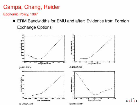
Campa, Chang, ReiderEconomic Policy, 1997

ERM Bandwidths for EMU and after: Evidence from ForeignExchange Options

This content downloaded from 130.223.2.2 on Sat, 31 Jan 2015 13:09:01 PMAll use subject to JSTOR Terms and Conditions

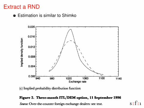
Extract a RNDEstimation is similar to Shimko


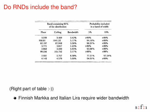
Do RNDs include the band?

This content downloaded from

130.223.2.2 on Sat, 31 Jan 2015 13:09:01 PMA

ll use subject to JSTOR Term

s and Conditions

(Left part of table :-))

Do RNDs include the band?

This content downloaded from

130.223.2.2 on Sat, 31 Jan 2015 13:09:01 PMA

ll use subject to JSTOR Term

s and Conditions

(Right part of table :-))

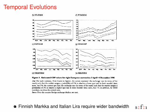
Finnish Markka and Italian Lira require wider bandwidth

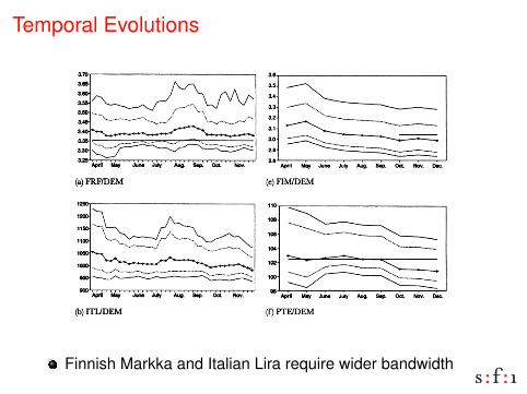
Temporal Evolutions



Former Gerzensee Participants: RNDs from BrazilianInterest Rate Options, 2009

Electronic copy available at: http://ssrn.com/abstract=1395503

Recovering Risk-Neutral Densities from Brazilian Interest Rate Options

José Renato Haas Ornelas

Banco Central do Brasil*

[email protected]

Marcelo Yoshio Takami

Banco Central do Brasil

[email protected]

ABSTRACT

Building Risk-Neutral Density (RND) from options data is one useful form of

extracting market expectations about a financial variable. For a sample of IDI

(Brazilian Interbank Deposit Rate Index) options from 1998 to 2009, this paper

estimates the option-implied Risk-Neutral Densities for the Brazilian short rate using

three methods: Shimko, Mixture of Two Log-Normals and Generalized Beta of Second

Kind. Our in-sample goodness-of-fit evaluation shows that the Mixture of Log-Normals

method provides better fitting to option’s data than the other two methods during the

our sample period. The shape of the family of log-normal distributions seems to fit well

to the mean-reversal dynamics of Brazilian interest rates. We also calculate the RND

implied Skewness, showing how it could have provided market early-warning signals of

the monetary policy outcomes in 2002 and 2003. Overall, Risk-Neutral Densities

implied on IDI options showed to be a useful tool for extracting market expectations

about future outcomes of the monetary policy.

KEY WORDS: Risk-Neutral Density, Interest Rate Options, Generalized Beta, Mixture of Log-Normals. JEL CLASSIFICATION: C13, C16, E47, E52, G12, G13, G17. 1. Introduction

Many techniques have been applied in order to extract market expectations. Building Risk-Neutral Density (RND) from options data is one of them. This information may be useful for financial stability analysis. Supervisory institutions can assess monetary policy impacts on expectations by inferring whether the market is attributing a high probability of a significant change on financial variables, such as interest rate or exchange rate. On the other way, market expectations on financial variables may influence monetary policy decisions. Using option-implied RND, one can calculate, for example, the probability that interest rate will stay inside a specific range of values.

* The views expressed in this work are those of the authors and do not reflect those of the Banco Central do Brasil or its members.


Former Gerzensee Participants: RNDs for ExchangeRate Options: Evidence for Turkey, 2009!"#$%"&'()*!'+,-."/0&12*3"(+'0'"+*4&$5*67#81()"*!10"*9:0'$(+;*6%'<"(#"*

'(*=/&,">?*!

@12'2* A&18'5*B><!( *Central Bank of the Republic of Turkey

B85"0*3" "&2'*

Central Bank of the Republic of Turkey!*

C!(1&*DE2F*Central Bank of the Republic of Turkey

***

BA+0&1#0*"#$%!&'&()!*%(%!+,()-.#(-/+*0.()!/*))(0/1!+&.$+0%!2'.'!.+!$0,(%.$3'.(!4')5(.!(6&(/.'.$+0%!+0!"*)5$%#! 7$)'-89:9! ;+<<')! (6/#'03(! )'.(9! =(! (6.)'/.! +&.$+0! $4&<$(2! 2(0%$.1! >*0/.$+0%! .+!(6'4$0(!.#(!(,+<*.$+0!+>!4')5(.!%(0.$4(0.!+,()!.#(!&+%%$?<(!,'<*(%!+>!>*.*)(!(6#'03(!)'.(%9!80/().'$0.1!$%!@(<<!4('%*)(2!?1!+&.$+0-$4&<$(2!&)+?'?$<$.$(%9!A%.$4'.(2!2(0%$.$(%!>+)!%(<(/.(2!2'1%! &+$0.! +*.! '0! $0/)('%(! $0! *0/().'$0.1! $0! >+)($30! (6/#'03(! 4')5(.! 2*)$03! >$0'0/$'<!.*)?*<(0/(!&()$+2%9!=(!4'5(! $0>()(0/(%!'?+*.! .#(!(>>(/.$,(0(%%!+>!&+<$/1!4('%*)(%!'02!%((!#+@! .#(!4')5(.! &()/(&.$+0! /#'03(2! .#)+*3#+*.! .#(! /)$%$%9!=(! *0/+,()! .#(! (>>(/.$,(0(%%! +>!&+<$/1!4('%*)(%!?1!+?%(),$03!%#)$05$03!2(0%$.$(%!'02!/+0>$2(0/(!?'02%9!

!

!

B(1@+)2%C!D&.$+0%E!F$%5!0(*.)'<!2(0%$.1E!G')5(.!(6&(/.'.$+0%9!!

!!

HA7!I+2(%C!JKLE!JKME!NLK!

!

**********

*

!!!!!!!!!!!!!!!!!!!!!!!!!!!!!!!!!!!!!!!!!!!!!!!!!O!"#$%!&'&()!#'%!?(0(>$.(2!>)+4!F(>(.!JP)5'10'5Q%!/+44(0.%9!=(!')(!3)'.(>*<!.+!:(<$4!A<(52' E!RS3P)!RS(<!'02!JP)%*!B(<( !>+)!#(<&>*<!/+44(0.%!+0!'!&)(,$+*%!2)'>.9!"#(!,$(@%!(6&)(%%(2!$0!.#$%!&'&()!2+!0+.!0(/(%%')$<1!)(&)(%(0.!.#+%(!+>!.#(!I(0.)'<!T'05!+>!.#(!F(&*?<$/!+>!"*)5(19!U<<!)(4'$0$03!())+)%!')(!+*)%9!!I+))(%&+02$03!'*.#+)C!V'<$<! ?)'#$4!U12!0W!F(%(')/#!'02!G+0(.')1!X+<$/1!;(&').4(0.E!ITF"W!V('2!D>>$/(!Y%.$5<'<!I'22(%$C!Z+9K[!8<*%W!U05')'W!"8FBA\![]K[[W!(-4'$<C!#'<$<9'12$0^./4?93+,9.)W!&#+0(C!_LK`a!LK[L]b]W!>'6C!_LK`a!L`b[MMc9!

Second GenerationAït-Sahalia, Lo: Nonparametric Risk Management and Implied Risk Aversion,JE’metrics 2000

Fig. 2.

and the "rst derivative of S-VaR. Bandwidth values to estimate fK H! and fK ! arereported in Table 4, and we plot the implied relative risk aversion function inFig. 4. The con"dence interval is constructed from the asymptotic distributiontheory derived in Proposition 4.

The notable feature of Fig. 4 is that "( exhibits a U-shaped pattern asa function of S

!. In other words, the market prices of S&P 500 options and the

market returns on the S&P 500 index are such that the representative agentbecomes more averse as the index goes down in value, as well as for very highvalues of the index. This phenomenon cannot be captured by CRRA preferences[see (5.7)], providing yet another characterization of the di!erences betweenmarket prices and the Black}Scholes model. Note also that the estimated "( inFig. 4 is everywhere positive, thereby implying a concave utility function.

Comparing the line (5.7) to the nonparametric estimate of "( in Fig. 4 providesa comparison of the constant CRRA preference, where ""a is constant, to thenonparametrically implied function of relative risk aversion. We "nd that theCRRA ranges between 1 and 60, depending upon the level of the S&P 500, i.e.,aggregate wealth. The weighted average, over the range of S&P 500 values, ofthe function "( is 12.7 and is represented by the horizontal line in Fig. 4. Aninteresting comparison is whether this range of values for a is `reasonablya

Y. An(t-Sahalia, A.W. Lo / Journal of Econometrics 94 (2000) 9}51 35

Theory

Representative agent who maximizes his lifetime utility

max{C0,C1,··· }

E0

[ ∞∑t=0

βt U(Ct)

]s.t.: Wt+1 = (Wt − Ct)Rt,t+1

Yields as first order condition

Et

[β

U ′(Ct+1)

U ′(Ct)Rt,t+1

]= 1

⇒∫

Ct+1,St+1

βU ′(Ct+1)

U ′(Ct)

St+1

Stp(Ct+1,St+1)dCt+1 dSt+1 = 1

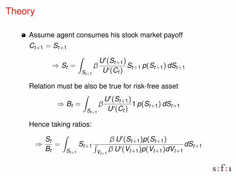
Theory

Assume agent consumes his stock market payoffCt+1 = St+1

⇒ St =

∫St+1

βU ′(St+1)

U ′(Ct)St+1 p(St+1)dSt+1

Relation must be also be true for risk-free asset

⇒ Bt =

∫St+1

βU ′(St+1)

U ′(Ct)1 p(St+1)dSt+1

Hence taking ratios:

⇒St

Bt=

∫St+1

St+1β U ′(St+1)p(St+1)∫

Vt+1β U ′(Vt+1)p(Vt+1)dVt+1

dSt+1

Theory

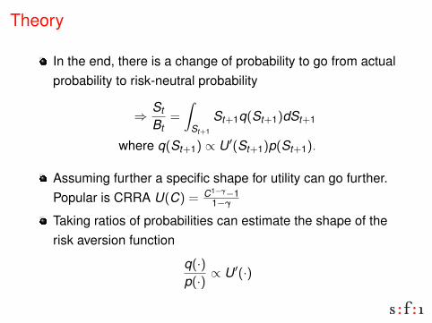
In the end, there is a change of probability to go from actualprobability to risk-neutral probability

⇒St

Bt=

∫St+1

St+1q(St+1)dSt+1

where q(St+1) ∝ U ′(St+1)p(St+1).

Assuming further a specific shape for utility can go further.Popular is CRRA U(C) = C1−γ−1

1−γ

Taking ratios of probabilities can estimate the shape of therisk aversion function

q(·)p(·) ∝ U ′(·)

Risk Aversion

Fig. 3.

compatible with the values found using consumption, but no option, data. Isthere an equity-premium-like puzzle at the levels of option prices, or do theyimply coe$cients of risk aversion that are less extreme than those typicallyfound in the equity-premium literature?!" This estimate for a is higher than thetypical values used in theoretical models (where the range is typically 1 to 5),higher than (!!r#")/#! (the value of a in the Black}Scholes model evaluatedat values of !, " and # given by the S&P 500 returns and the riskfree rate r), yetgenerally lower than the estimates found by studies of the Euler equation inconsumption-based asset pricing models.!# Table 5 reports the range of valuesof the constant CRRA that have been estimated in the literature. While theimplied CRRA coe$cient is informative, it is important to keep in mind that

!"See Renault and Garcia (1996) for a di!erent attempt to confront option data with the Eulerequation.

!#However, it should be emphasized that our estimate is based on nominal data, whereasestimates obtained from consumption-based asset-pricing models use real data. For our relativelyshort time-horizon (less than one year), this distinction may not matter; see footnote 14 for furtherdiscussion.

36 Y. An(t-Sahalia, A.W. Lo / Journal of Econometrics 94 (2000) 9}51

Why the hump?

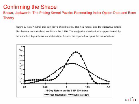
Confirming the ShapeBrown, Jackwerth: The Pricing Kernel Puzzle: Reconciling Index Option Data and EconTheory

!"

#$%&'(")*"+$,-./(&0'12" 134"5&67(80$9(":$,0'$6&0$;3,*"<=(" '$,-.3(&0'12" 134" 0=(" ,&67(80$9(" '(0&'3"

4$,0'$6&0$;3,"1'("8128&210(4";3">1'8="?@A"?!!B*"<=(",&67(80$9("4$,0'$6&0$;3" $,"1CC';D$E10(4"6F"

0=(",E;;0=(4"G.F(1'"=$,0;'$812"4$,0'$6&0$;3*"+(0&'3,"1'("'(C;'0(4"1,"?"C2&,"0=("'10(";H"'(0&'3*"

"

!

"

#

$

%

&

'

(

)

!*+ !*+& " "*!& "*"$",-./0123456076038209:;0&!!0<6=2>

?0;57@.@<A<3/

1<BC,D2435.A0EFGH 94@I2J3<K20ELGH"

"

I"0FC$812"(,0$E10(";H""EA",1F""EJA"1CC(1',"$3"#$%&'("K"1,"1"H&380$;3";H"0=("'(0&'3";3"0=("

5LM"NBB"$34(D*"+;,(36('%"134"O3%2("P)BB)Q"8;3H$'E"0=$,",=1C("6F"&,$3%"1"'(210(4"E(0=;4A"134"

R18-S('0="P)BBGQ"C';9$4(,"$30('310$;312"(9$4(38("H;'"T('E13FA"R1C13A"134"0=("UV*W""

"""""""""""""""""""""""""""""""""""""""""""""""""W"X3"1"H&'0=('"(DC2;'10;'F",0&4FA"S("$39(,0$%10(4"E1'-(0"H'$80$;3,"$3"1"T>>",(00$3%",01'0$3%"S$0="0=("O&2('"(Y&10$;3"OZE" '[" \" ?*"](" &,(" 0=(" 4101,(0" ;3" ;C0$;3," '(0&'3," H';E"^&'1,8=$" 134" R18-S('0=" P)BB?Q*"_(" 134">;4(,0" P?!!NQ",&%%(,0"0=10"0=("9(80;'";H""?`,"",=;&24"6("'(C218(4"S$0=",;E(";0=('"912&(A"82;,("0;""?""H;'"0'13,180$;3"8;,0,";'"2(,,"0=13" ?" H;'" ,=;'0" ,12(" 8;3,0'1$30,*" _;S(9('A" 1," 0=(" E1'%$312" $39(,0;'" P0=(" ;3(" S$0=" 0=(" 2;S(,0" 8;,0,Q" ,(0," 0=("(Y&$2$6'$&E"C'$8(,A"$0"$,"=1'4"0;"$E1%$3("0=10"0=("9(80;'",=;&24"6("91,02F"4$HH('(30"H';E""?a"(,C(8$122F",$38("0=("E1'-(0"E1-('"134"0=("0'14(',"1'("3;0",=;'0",12("8;3,0'1$30*"]("3((4"0;"&,("13"(DC(80(4"912&(";H"0=("b<>"C&0"'(0&'3,A"S=$8="$,",;E(""GB.NB""61,$,"C;$30,"2;S('"0=13""?A"$3";'4('"0;"18=$(9("1"E;3;0;3$8122F"4(8'(1,$3%"C'$8$3%"-('3(2*"5&8="21'%("41$2F"0'13,180$;3"8;,0"$,"=1'4"0;"$E1%$3("$3"0=$,"2$Y&$4"E1'-(0*"5&8="4$E$3$,=(4"'(0&'3"8;&24"12,;",&%%(,0"E$,C'$8$3%A"1"C;,$0$;3"(DC2;'(4"$3"R18-S('0="P)BBBQ"134",&CC;'0(4"6F"I%1'S12"134"/1$-"P)BBBQA"S=;"H$34"0=10"=(4%("H&34,"0(34"0;",(22";&0.;H.0=(.E;3(F"134"10.0=(.E;3(F"C&0,*"^;341'(3-;"P)BBKQA"c;912"134"5=&ES1F"P)BB?QA"134":'$(,,(3"134">1(3=;&0"P)BBKQ"12,;"H$34" 0=10",$E$21'";C0$;3" 0'14$3%",0'10(%$(," 0&'3";&0" 0;"6("9('F"C';H$0162(*"T$9(3" 0=(",$d("134"2$Y&$4$0F";H"0=$,"E1'-(0A";&'"C'$;'"$,"=;S(9('A"0=10",&8="C';H$0";CC;'0&3$0$(,",=;&24"3;0"(D$,0"H;'"0(3"F(1',"S$0=;&0"13F"0(34(38F"0;S1'4,"(Y&$2$6'$&E*"

Confirming the Shape

!"#

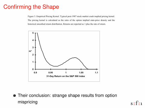
$%&'()#*+#,-.%(%/01#2(%/%3&#4)(3)1+#56.%/01#.789:!;<=#897/>#-0(>)9#/(08?#%-.1%)@#.(%/%3&#>)(3)1+#

5?)# .(%/%3&# >)(3)1# %8# /01/'109)@# 08# 9?)# (09%7# 7A# 9?)# 7.9%73# %-.1%)@# 8909):.(%/)# @)38%96# 03@# 9?)#

?%897(%/01#8-779?)@#()9'(3#@%89(%B'9%73+#C)9'(38#0()#().7(9)@#08#!#.1'8#9?)#(09)#7A#()9'(3+#

#

!

"

#

$

%

&

!'( !'(& " "'!& "'"$")*+,-./0123-43-05/-678-&!!-93:/;

<=

#

#

$7(#036#7.9%73:.(%/%3&#-7@)1D#9?)#.179#7A#9?)#>)(3)1##-##E08#%3#$%&'()#*F#%8#/178)16#9%)@#97#

9?)#@)&())#7A# 9?)# 8-%1)# E1%>)# 9?09#7A#$%&'()#!F+;# G9# %8# %-.7(9039# 97#379)# 9?09# 036#-7@)1#'8)@# 97#

)H.10%3#9?)#8-%1)#%3#9?)#IJ2#K""#%3@)H#7.9%738#-'89#.(7L%@)#0#>)(3)1##-##9?09#%8#/738%89)39#M%9?#

$%&'()#*+#5?09#%8D#9?)#>)(3)1#%-.1%)@#B6#0#M)11:/7389('/9)@#-7@)1#-'89#?0L)#0#/)39(01#(03&)#9?09#

%8# %3/()08%3&#M%9?# 9?)# %3@)H+# 5?)# &701# 7A# 9?%8#M7(># %8# 97# A%3@#-7@)18# 9?09# )H.10%3# 9?)# .(%/%3&#

>)(3)1#08#8?7M3#%3#$%&'()#*+#5?)#L01')#7A# #!## %3#9?)#/)39)(#7A#9?)#?7(%N73901#0H%8#().()8)398#03#

)3@%3&#1)L)1#7A#9?)#%3@)H#E%+)+D#09#9?)#9%-)#7A#7.9%73#)H.%(09%73F#9?09#%8#)O'01#97#9?)#/'(()39#1)L)1#

E09# 9?)#B)&%33%3&#7A#9?)#*!:@06#%39)(L01F+#P17B0116D##-Q##%8#0#@)/()08%3&#A'3/9%73#7A#9?)#)3@%3&#

%3@)H#1)L)1+#R7M)L)(D#A7(#9?)#(03&)#A(7-#0..(7H%-09)16##"+;=##97##!+"*D#%+)+#A7(#0#(03&)#7A#%3@)H#

1)L)18#/)39)()@#73#03@#M%9?%3#0# #*S##@)L%09%73#A(7-#9?)#/'(()39# 1)L)1D# #-Q## %8# %3/()08%3&+#5?%8#

#################################################;#T)# @7# 379# A7(-0116# @)-7389(09)# 9?)# 1%3># B)9M))3# .1798# 7A# #-# # 03@# 8-%1)8# ?)()D# B'9# ()A)(# 97# 9?)# @%8/'88%73# %3#U0/>M)(9?#EV"""F#03@#C78)3B)(&#03@#,3&1)#EV""VF+#

Their conclusion: strange shape results from optionmispricing

Recent Implementations of RNDs

My dream come true

https://www.minneapolisfed.org/banking/mpd

Birru and Figlewski: The Impact of the Federal Reserve’sInterest Rate Target Announcement on Stock Prices: ACloser Look at How the Market Impounds New Information,2010

Allan Malz: 2013, Risk-Neutral Systemic Risk Indicators.

week 1 - gerzensee · week 1 michael rockinger ... rate and a forward rate agreement (fra) ... that...

Documents