MRP Materials Reliability Program_____________________________MRP 2007-034 (via email) Page 1 of 2 July 31, 2007 James Riley Nuclear Energy Institute 1776 I Street, NW, Ste. 400 Washington, DC 20006 Subject: Transmittal of EPRI Report MRP-216, Advanced FEA Evaluation of Postulated Circumferential Flaws in Pressurizer Nozzle Dissimilar Metal Welds Dear Mr. Riley: All technical work on the Advanced Finite Element Project has been completed and the final report will be submitted for formal publication by EPRI. This report titled “Advanced FEA Evaluation of Growth of Postulated Circumferential PWSCC Flaws in Pressurizer Nozzle Dissimilar Metal Welds (MRP-216): Evaluations Specific to Nine Subject Plants” is attached. We recognize the need for immediate release of this report to support licensing and regulatory decisions. In order to accommodate this need and the necessary elements of publishing an EPRI report, we are publishing this report in the following manner. The pre-publication technically complete version attached to this letter provides comprehensive documentation of the entire project and the analytical results for immediate use by all interested parties. The EPRI Technical Publication department is responsible for publishing, maintaining, and archiving EPRI technical information which represents the intellectual property of the Institute. One of the primary jobs of technical publishing is to provide consistent formatting to help capture critical content in a way that is vital for building comprehensive knowledge management systems. In addition, reviews are performed to ensure that all documents have the EPRI background statement, copyright information, export control, and legal and liability disclaimers. The publishing process does not in any way alter the technical content or conclusions of the research. We understand that NEI will formally transmit the attached report to NRC. In addition, the NEI transmittal letter should be the reference for further licensee correspondence on the Confirmatory Action Letters. Following these activities, EPRI Technical Publishing will expedite the subsequent formal release of the document first as a Technical Update report by August 3, 2007 through an abbreviated publishing process followed by a final published Technical Report by August 24, 2007. These will be formal, referable, EPRI products. Please note that this entire project has been conducted in a very public and open manner with essentially all documents freely released. Therefore, this report is being issued as “Copyright Only” and thus no license agreement is required, only proper attribution when this work is used or referenced. Should you have questions regarding this report, please contact me. Craig Harrington Sr. Project Manager EPRI MRP

MRP Materials Reliability Program_____________________________MRP 2007-034 (via email) Page 2 of 2 Attachment cc: E Sullivan, NRC A Csontos, NRC Research W Borrero, APS G DeBoo, Exelon M Dove, Southern Co. L Goyette, PG&E T McAlister, SCANA V Penacerrada, Entergy W Sims, Entergy D Sutton, Southern Co C Tran, TXU Energy J Thayer, NEI A Marion, NEI M Melton, NEI D Modeen, EPRI R Yang, EPRI D Steininger, EPRI C King, EPRI D Weakland, First Energy W Bamford, Westinghouse D Harris, Structural Integrity Associates D Killian, AREVA P Riccardella, Structural Integrity Associates K Yoon, AREVA T Gilman, Structural Integrity Associates

EPRI Project Managers C. Harrington C. King

EPRI • 3412 Hillview Avenue, Palo Alto, California 94304 • PO Box 10412, Palo Alto, California 94303 • USA 800.313.3774 • 650.855.2121 • askepri@epri.com • www.epri.com

Advanced FEA Evaluation of Growth of Postulated Circumferential PWSCC Flaws in Pressurizer Nozzle Dissimilar Metal Welds (MRP-216) Evaluations Specific to Nine Subject Plants 1015383

Pre-Publication Version, July 31, 2007

DISCLAIMER OF WARRANTIES AND LIMITATION OF LIABILITIES

THIS DOCUMENT WAS PREPARED BY THE ORGANIZATION(S) NAMED BELOW AS AN ACCOUNT OF WORK SPONSORED OR COSPONSORED BY THE ELECTRIC POWER RESEARCH INSTITUTE, INC. (EPRI). NEITHER EPRI, ANY MEMBER OF EPRI, ANY COSPONSOR, THE ORGANIZATION(S) BELOW, NOR ANY PERSON ACTING ON BEHALF OF ANY OF THEM:

(A) MAKES ANY WARRANTY OR REPRESENTATION WHATSOEVER, EXPRESS OR IMPLIED, (I) WITH RESPECT TO THE USE OF ANY INFORMATION, APPARATUS, METHOD, PROCESS, OR SIMILAR ITEM DISCLOSED IN THIS DOCUMENT, INCLUDING MERCHANTABILITY AND FITNESS FOR A PARTICULAR PURPOSE, OR (II) THAT SUCH USE DOES NOT INFRINGE ON OR INTERFERE WITH PRIVATELY OWNED RIGHTS, INCLUDING ANY PARTY'S INTELLECTUAL PROPERTY, OR (III) THAT THIS DOCUMENT IS SUITABLE TO ANY PARTICULAR USER'S CIRCUMSTANCE; OR

(B) ASSUMES RESPONSIBILITY FOR ANY DAMAGES OR OTHER LIABILITY WHATSOEVER (INCLUDING ANY CONSEQUENTIAL DAMAGES, EVEN IF EPRI OR ANY EPRI REPRESENTATIVE HAS BEEN ADVISED OF THE POSSIBILITY OF SUCH DAMAGES) RESULTING FROM YOUR SELECTION OR USE OF THIS DOCUMENT OR ANY INFORMATION, APPARATUS, METHOD, PROCESS, OR SIMILAR ITEM DISCLOSED IN THIS DOCUMENT.

ORGANIZATION(S) THAT PREPARED THIS DOCUMENT

Dominion Engineering, Inc. (Except Appendices)

Structural Integrity Associates, Inc. (Appendices B, D, and E)

Quest Reliability, LLC (Appendix C)

Westinghouse Electric Co. (Appendix A)

ORDERING INFORMATION

Requests for copies of this report should be directed to EPRI Orders and Conferences, 1355 Willow Way, Suite 278, Concord, CA 94520. Toll-free number: 800.313.3774, press 2, or internally x5379; voice: 925.609.9169; fax: 925.609.1310.

Electric Power Research Institute and EPRI are registered service marks of the Electric Power Research Institute, Inc. EPRI. ELECTRIFY THE WORLD is a service mark of the Electric Power Research Institute, Inc.

Copyright © 2007 Electric Power Research Institute, Inc. All rights reserved.

iii

CITATIONS

This report (except appendices) was prepared by

Dominion Engineering, Inc. 11730 Plaza America Drive Suite 310 Reston, VA 20190

Principal Investigators G. A. White J. E. Broussard

Contributors J. E. Collin M. T. Klug D. J. Gross V. D. Moroney The authors of each of the appendices are identified on the first page of each respective appendix.

This report describes research sponsored by EPRI.

The report is a corporate document that should be cited in the literature in the following manner:

Advanced FEA Evaluation of Growth of Postulated Circumferential PWSCC Flaws in Pressurizer Nozzle Dissimilar Metal Welds (MRP-216): Evaluations Specific to Nine Subject Plants, EPRI, Palo Alto, CA: 2007. 1015383.

v

REPORT SUMMARY

Indications of circumferential flaws in the pressurizer nozzles at Wolf Creek raised questions about the need to accelerate refueling outages or take mid-cycle outages at other plants. This study demonstrates the viability of leak detection as a means to preclude the potential for rupture for the pressurizer nozzle dissimilar metal (DM) welds in a group of nine PWRs originally scheduled to perform performance demonstration initiative (PDI) inspection or mitigation during the spring 2008 outage season. Modeling showed that the classical assumption of a semi-elliptical crack shape results in a large overestimation of the crack area and thus an underestimation of crack stability at the time when the crack penetrates to the outside surface.

Background In October 2006, several indications of circumferential flaws were reported in the pressurizer nozzles at Wolf Creek. The indications were located in the nickel-based Alloy 82/182 dissimilar metal (DM) weld material, which is known to be susceptible to primary water stress corrosion cracking (PWSCC). During its fall 2006 outage, Wolf Creek addressed the concern for growth of these circumferential indications through application of previously scheduled weld overlays. In late 2006, the Materials Reliability Program (MRP) performed a series of short-term evaluations of the implications of the Wolf Creek indications for other PWR plants. This study extends the crack growth calculations of these short-term evaluations to consider flaw shape development based on the crack-tip stress intensity factor calculated at each point along the crack front.

Objective To evaluate the viability of detection of leakage from a through wall flaw in an operating plant to preclude the potential for rupture of pressurizer nozzle DM welds in the group of nine PWRs originally scheduled for performance demonstration initiative (PDI) inspection or mitigation during the spring 2008 outage season, given the potential concern about growing circumferential stress corrosion cracks.

Approach In order to facilitate modeling of the crack shape development, Quest Reliability, LLC extended its FEACrack software to model the growth of circumferential flaws having a custom profile. In Phase I of this study, the team applied this new software tool to the same basic weld geometry, piping load inputs, and welding residual stress distribution assumed in the late 2006 MRP calculation. In Phase II, the team investigated an extensive crack growth sensitivity matrix to cover the geometry, load, and fabrication factors for each of the 51 subject welds, as well as the uncertainty in key modeling parameters including the effect of multiple flaw initiation sites in a single weld. Other key Phase II activities included detailed welding residual stress simulations

vi

covering the subject welds, development of a conservative crack stability calculation methodology, development of a leak rate calculation procedure using existing software tools (EPRI PICEP and NRC SQUIRT), and verification and validation studies.

Results Based on the detailed input of an EPRI-led expert panel, researchers developed a set of criteria to evaluate the results of the crack growth, crack stability, and leak rate calculations for each sensitivity case investigated. The evaluation criteria provide safety margins based on explicit consideration of leak rate detection sensitivity, plant response time, and uncertainty in the crack stability calculations. An extensive sensitivity matrix of 119 cases was developed to robustly address the weld-specific geometry, load input parameters for the set of 51 subject welds, plus the key modeling uncertainties. All 109 cases in the main sensitivity matrix showed either stable crack arrest (60 cases) or crack leakage and crack stability results satisfying the evaluation criteria (49 cases). In most cases, the results showed large evaluation margins in leakage time and in crack stability. Ten supplemental cases added to further investigate the potential effect of multiple flaws in the subject surge nozzles also satisfied the evaluation criteria with the exception of two cases that involved initial flaw assumptions that are not credible.

An additional key finding concerns the significant number of crack growth sensitivity cases that showed stable crack arrest prior to through-wall penetration. This type of behavior is consistent with the relatively narrow band of relative depths reported for the four largest Wolf Creek indications. Also, detailed evaluations tend to support the relaxation of piping thermal constraint stresses prior to rupture, but such relaxation was conservatively not credited in the base assumptions of the critical crack size methodology developed for this study. Instead, 100% of the normal operating thermal piping loads (excluding surge line thermal stratification effects) was included in the critical crack size calculations.

EPRI Perspective This study extends the state-of-the-art regarding modeling of PWSCC crack growth. EPRI report 1006696 (MRP-115), which developed a deterministic crack growth rate equation as a function of stress intensity factor on the basis of worldwide laboratory testing of controlled fracture mechanics specimens, provided key input to the crack growth calculations of this study. The crack growth methodology developed in support of this study may be applied in similar future applications for PWR components outside of the pressurizer. EPRI report 1010087 (MRP-139) defines inspection and evaluation requirements for DM (Alloy 82/182) welds in U.S. PWRs. EPRI report 1011808 (MRP-140) evaluates previous regulatory leak-before-break (LBB) submittals to the U.S. NRC given the potential for the presence of PWSCC at Alloy 82/182 locations.

Keywords Alloy 600 Alloy 82/182 Crack growth modeling Dissimilar metal piping butt/girth welds Leak before break (LBB) Pressurizer nozzles Primary water stress corrosion cracking (PWSCC)

vii

ABSTRACT

In October 2006, several indications of circumferential flaws were reported in the Wolf Creek pressurizer nozzles. The indications were reported to be located in the nickel-based Alloy 82/182 dissimilar metal (DM) weld material, which is known to be susceptible to primary water stress corrosion cracking (PWSCC). In late 2006, the Materials Reliability Program (MRP) performed a series of short-term evaluations of the implications of the Wolf Creek indications for other PWR plants. This study extends the crack growth calculations of the short-term evaluations to consider flaw shape development based on the crack-tip stress intensity factor calculated at each point along the crack front.

The objective of this study is to evaluate the viability of operating plant leak detection, from a through-wall flaw perspective, to preclude the potential for rupture for the pressurizer nozzle DM welds in the group of nine PWRs originally scheduled to perform PDI inspection or mitigation during the spring 2008 outage season, given the potential concern for growing circumferential stress corrosion cracks. Commitments have been made for these nine PWRs to accelerate refueling outages or take mid-cycle outages. Should this study demonstrate flaw stability via sufficient time from initial detectable leakage until pipe rupture, as demonstrated to the NRC, these plants could then resume plans to perform PDI inspection or mitigation during the spring 2008 outage season. In Phase I of this study, newly enhanced FEACrack software tools were applied to the same basic weld geometry, piping load inputs, and welding residual stress distribution assumed in the late 2006 MRP calculation. In Phase II, an extensive crack growth sensitivity matrix of 119 cases was investigated to robustly address the geometry, load, and fabrication factors for each of the 51 subject welds, as well as the uncertainty in key modeling parameters including the effect of multiple flaw initiation sites in a single weld. Other key Phase II activities included detailed welding residual stress simulations, development of a conservative crack stability calculation methodology, development of a leak rate calculation procedure using existing software tools, and verification and validation studies.

This study demonstrated that the classical assumption of a semi-elliptical crack shape results in a large overestimation of the crack area and thus underestimation of the crack stability at the point in time at which the crack penetrates to the outside surface. All 109 cases in the main sensitivity matrix showed either stable crack arrest (60 cases) or crack leakage and crack stability results satisfying the evaluation criteria (49 cases). In most cases, the results showed large evaluation margins in leakage time and in crack stability. Ten supplemental cases were added to further investigate the potential effect of multiple flaws in the subject surge nozzles. With the exception of two cases that involved initial flaw assumptions that are not credible (as discussed in the report), the supplemental sensitivity cases also satisfied the evaluation criteria. In summary, this study demonstrated the viability of leak detection to preclude the potential for rupture for the subject pressurizer nozzle DM welds.

ix

ACKNOWLEDGMENTS

This study was completed with the detailed support and input of the expert review panel assembled by EPRI and of utility reviewers:

EPRI Project Management and Support

C. Harrington (EPRI), C. King (EPRI), and T. Gilman (Structural Integrity Associates)

EPRI Expert Review Panel

T. Anderson (Quest Reliability, LLC), W. Bamford (Westinghouse), D. Harris (Structural Integrity Associates), D. Killian (AREVA), P. Riccardella (Structural Integrity Associates), and K. Yoon (AREVA)

Utility Reviewers

W. Borrero (APS), G. DeBoo (Exelon), M. Dove (Southern Co.), L. Goyette (PG&E), T. McAlister (SCANA), M. Melton (NEI), V. Penacerrada (Entergy), W. Sims (Entergy), D. Sutton (Southern Co.), and C. Tran (TXU Energy)

In direct support of this study, Quest Reliability, LLC extended its FEACrack software to model the growth of circumferential flaws having a custom profile. G. Thorwald and D. Revelle led the software development effort at Quest Reliability, LLC.

xi

ACRONYMS

The following acronyms are used in the main body of this report:

ANSC (Structural Integrity Associates) Arbitrary Net Section Collapse software ASME American Society of Mechanical Engineers CE Combustion Engineering CGR crack growth rate CMTR certified material test report COA crack opening area COD crack opening displacement DEI Dominion Engineering, Inc. DM dissimilar metal DMW dissimilar metal weld DPZP dimensionless plastic zone parameter EMC2 Engineering Mechanics Corporation of Columbus EPFM elastic-plastic fracture mechanics EPRI Electric Power Research Institute FEA finite-element analysis ID inside diameter IGSCC intergranular stress corrosion cracking LBB leak before break MRP Materials Reliability Program ND neutron diffraction NDE non-destructive examination NRC Nuclear Regulatory Commission NSC net section collapse NSSS nuclear steam supply system OD outside diameter PDI performance demonstration initiative PICEP (EPRI) Pipe Crack Evaluation Program PWR pressurized water reactor PWSCC primary water stress corrosion cracking RCS reactor coolant system SCC stress corrosion cracking SIF stress intensity factor SQUIRT (NRC) Seepage Quantification of Upsets in Reactor Tubes UT ultrasonic testing WRS welding residual stress

xiii

CONTENTS

1 INTRODUCTION ....................................................................................................................1-1 1.1 Background .....................................................................................................................1-1

1.1.1 Fall 2006 Wolf Creek Inspection Results and MRP White Paper............................1-1 1.1.2 December 2006 Crack Growth Evaluations ............................................................1-1

1.2 Objective .........................................................................................................................1-2 1.3 Scope ..............................................................................................................................1-2 1.4 Approach.........................................................................................................................1-3 1.5 Expert Panel....................................................................................................................1-3 1.6 Report Structure..............................................................................................................1-3

2 PLANT INPUTS......................................................................................................................2-1 2.1 Geometry Cases .............................................................................................................2-1

2.1.1 Safety/Relief Nozzles ..............................................................................................2-1 2.1.2 Spray Nozzles .........................................................................................................2-1 2.1.3 Surge Nozzles .........................................................................................................2-2

2.2 Piping Load Inputs...........................................................................................................2-2 2.2.1 Pressure, Dead Weight, and Normal Thermal Loads..............................................2-2 2.2.2 Surge Line Thermal Stratification Effects ................................................................2-2

2.3 Weld Fabrication .............................................................................................................2-3 2.3.1 “Back-Weld” Process...............................................................................................2-3 2.3.2 “Machined” Process.................................................................................................2-4

2.4 Weld Repair History ........................................................................................................2-4

3 WELDING RESIDUAL STRESS ............................................................................................3-1 3.1 Finite Element Analysis of Welding Residual Stress.......................................................3-1

3.1.1 Cases Considered ...................................................................................................3-1 3.1.2 FEA Modeling and Methodology .............................................................................3-2 3.1.3 Analysis Results ......................................................................................................3-7

xiv

3.2 WRS Literature Data .......................................................................................................3-9 3.3 Validation and Benchmarking..........................................................................................3-9

4 CRACK GROWTH MODELING .............................................................................................4-1 4.1 Modeling Approach .........................................................................................................4-1

4.1.1 FEA Model...............................................................................................................4-1 4.1.2 Calculation of Crack Tip Stress Intensity Factor .................................................4-3 4.1.3 Crack Growth for an Arbitrary Flaw Shape .........................................................4-4 4.1.4 Flaw Shape Transition ........................................................................................4-5

4.2 Fracture Mechanics Calculation Software Background...................................................4-5 4.3 Extensions to Fracture Mechanics Software ...................................................................4-6 4.4 Phase I Crack Growth Results ........................................................................................4-7

4.4.1 Preliminary Phase I Results ....................................................................................4-7 4.4.2 Phase I Results Using Final Mesh Parameters of Section 7 Sensitivity Matrix .......4-8

4.5 Stress Intensity Factor Verification..................................................................................4-9 4.6 Crack Growth Convergence Checks...............................................................................4-9

4.6.1 Temporal Convergence Check................................................................................4-9 4.6.2 Spatial Convergence Check ..................................................................................4-10

4.7 Validation Cases ...........................................................................................................4-10

5 CRITICAL CRACK SIZE CALCULATIONS...........................................................................5-1 5.1 Methodology....................................................................................................................5-1 5.2 Applied Loads..................................................................................................................5-2 5.3 Load Considerations .......................................................................................................5-2 5.4 EPFM Considerations .....................................................................................................5-3 5.5 Calculations Verification..................................................................................................5-4 5.6 Model Validation Comparison with Experiment...............................................................5-4

6 LEAK RATE MODELING .......................................................................................................6-1 6.1 PICEP Modeling..............................................................................................................6-1 6.2 Scoping Results ..............................................................................................................6-2 6.3 Comparison with SQUIRT Modeling ...............................................................................6-2 6.4 Leak Rate Predication Uncertainty..................................................................................6-3

7 SENSITIVITY CASE MATRIX ................................................................................................7-1 7.1 Modeling Procedure and Outputs....................................................................................7-1

xv

7.2 Evaluation Criteria ...........................................................................................................7-2 7.2.1 Introduction..............................................................................................................7-2 7.2.2 Criteria .....................................................................................................................7-3 7.2.3 Basis........................................................................................................................7-3 7.2.4 Application ...............................................................................................................7-5

7.3 Sensitivity Parameters.....................................................................................................7-6 7.3.1 Fracture Mechanics Model Type .............................................................................7-6 7.3.2 Geometry Cases......................................................................................................7-6 7.3.3 Piping Load Cases ..................................................................................................7-6 7.3.4 Welding Residual Stress Cases ..............................................................................7-7 7.3.5 K-Dependence of Crack Growth Rate Equation......................................................7-8 7.3.6 Initial Flaw Cases ....................................................................................................7-8 7.3.7 Consideration of Multiple Flaws...............................................................................7-9

7.4 Definition of Case Matrix .................................................................................................7-9 7.4.1 Geometry and Load Base Cases (1-20)..................................................................7-9 7.4.2 ID Repair Base Cases (21-26) ................................................................................7-9 7.4.3 Further Bending Moment Cases (27-30) ...............................................................7-10 7.4.4 Cases to Investigate Potential Uncertainty in As-Built Dimensions (31-32) ..........7-10 7.4.5 Axial Membrane Load Sensitivity Cases (33-34)...................................................7-10 7.4.6 Effect of Length Over Which Thermal Strain Simulating WRS is Applied (35) ......7-10 7.4.7 Simulation of Elastic-Plastic Redistribution of Stress at ID (36) ............................7-11 7.4.8 Effect of Initial Crack Shape and Depth (37-41) ....................................................7-11 7.4.9 Effect of Stress Intensity Factor Dependence of Crack Growth Rate Equation (42-47) ............................................................................................................................7-11 7.4.10 Effect of Pressure Drop Along Leaking Crack (48)..............................................7-12 7.4.11 Effect of Relaxation of Normal Operating Thermal Load (49-51) ........................7-12 7.4.12 Effect of Nozzle-to-Safe-End Crack Growth Model vs. Standard Cylindrical Crack Growth Model (52-53) ..........................................................................................7-12 7.4.13 Supplementary Cases Specific to Effect of Multiple Flaws on Limiting Surge Nozzles (S1-S9) .............................................................................................................7-13

7.5 Matrix Results................................................................................................................7-14 7.5.1 Geometry and Load Base Cases (1-20)................................................................7-15 7.5.2 ID Repair Base Cases (21-26) ..............................................................................7-15 7.5.3 Further Bending Moment Cases (27-30) ...............................................................7-15 7.5.4 Cases to Investigate Potential Uncertainty in As-Built Dimensions (31-32) ..........7-16 7.5.5 Axial Membrane Load Sensitivity Cases (33-34)...................................................7-16

xvi

7.5.6 Effect of Length Over Which Thermal Strain Simulating WRS is Applied (35) ......7-16 7.5.7 Simulation of Elastic-Plastic Redistribution of Stress at ID (36) ............................7-17 7.5.8 Effect of Initial Crack Shape and Depth (37-41) ....................................................7-17 7.5.9 Effect of Stress Intensity Factor Dependence of Crack Growth Rate Equation (42-47) ............................................................................................................................7-17 7.5.10 Effect of Pressure Drop Along Leaking Crack (48)..............................................7-17 7.5.11 Effect of Relaxation of Normal Operating Thermal Load (49-51) ........................7-18 7.5.12 Effect of Nozzle-to-Safe-End Crack Growth Model vs. Standard Cylindrical Crack Growth Model (52-53) ..........................................................................................7-18 7.5.13 Supplementary Cases Specific to Effect of Multiple Flaws on Limiting Surge Nozzles (S1-S9) .............................................................................................................7-18

7.6 Conclusions...................................................................................................................7-19 7.6.1 Main Sensitivity Matrix...........................................................................................7-19 7.6.2 Supplemental Sensitivity Matrix.............................................................................7-20 7.6.3 Tendency of Circumferential Surface Cracks to Show Stable Arrest ....................7-20 7.6.4 Nozzles with Liner Directly Covering Dissimilar Metal Weld .................................7-21 7.6.5 Potential Effect of Multiple Through-Wall Flaw Segments on Leak Rate ..............7-21 7.6.6 Overall Conclusion ................................................................................................7-22

8 SUMMARY AND CONCLUSIONS .........................................................................................8-1

9 REFERENCES .......................................................................................................................9-1

A APPENDIX A: DISSIMILAR METAL BUTT WELD FABRICATION PROCESSES............ A-1 A.1 General Pressurizer Nozzle Fabrication Processes ...................................................... A-1 A.2 Surge Nozzle Fabrication............................................................................................... A-6

A.2.1 Machined DM Weld Land with Rolled Thermal Sleeve .......................................... A-6 A.2.3 Back-Weld DM Weld Land with Welded Thermal Sleeve ...................................... A-8 A.2.3 Machined DM Weld Land with Welded Thermal Sleeve ...................................... A-11

A.3 Spray Nozzle Fabrication............................................................................................. A-13 A.4 Safety/Relief Nozzle Fabrication.................................................................................. A-14 A.5 Design Sketches.......................................................................................................... A-15

B APPENDIX B: EVALUATION OF THE EFFECTS OF SECONDARY STRESSES ON SURGE LINE CRITICAL FLAW SIZE CALCULATIONS ........................................................ B-1

B.1 Introduction .................................................................................................................... B-1 B.2 Full Scale Pipe Fracture Experiments............................................................................ B-2

xvii

B.2.1 Test Data................................................................................................................ B-2 B.2.2 Permissible Rotations ............................................................................................ B-2 B.2.3 Material Toughness................................................................................................ B-3

B.3 Surge Line Piping Analyses........................................................................................... B-4 B.3.1 Piping Models......................................................................................................... B-4 B.3.2 Loading Cases ....................................................................................................... B-4 B.3.3 Analysis Results..................................................................................................... B-5

B.4 Conclusions ................................................................................................................... B-5 B.5 References..................................................................................................................... B-6

C APPENDIX C: SECONDARY STRESS STUDY—PIPE BENDING WITH A THROUGH-THICKNESS CRACK............................................................................................ C-1

C.1 Introduction.................................................................................................................... C-1 C.2 Analysis ......................................................................................................................... C-1

C.2.1 Material Data.......................................................................................................... C-2 C.2.2 Imposed Rotation and Restrained Axial Extension................................................ C-2 C.2.3 Imposed Rotation and Unrestrained Axial Extension............................................. C-3

C.3 Summary ....................................................................................................................... C-3

D APPENDIX D: SCATTER IN LEAK RATE PREDICTIONS................................................. D-1 D.1 Evaluation...................................................................................................................... D-1 D.2 References .................................................................................................................... D-2

E APPENDIX E: EVALUATION OF PRESSURIZER ALLOY 82/182 NOZZLE FAILURE PROBABILITY ......................................................................................................... E-1

E.1 Introduction .................................................................................................................... E-1 E.2 Flaw Distributions........................................................................................................... E-2

E.2.1 Inspection Data ...................................................................................................... E-2 E.2.2 Statistical Fits to the Data ...................................................................................... E-3

E.3 Critical Flaw Size Distribution ........................................................................................ E-4 E.3.1 Applied Load Distribution ....................................................................................... E-4 E.3.2 Compilation of Full Scale Pipe Tests ..................................................................... E-5 E.3.3 Development of Fragility Curve.............................................................................. E-6

E.4 Crack Growth................................................................................................................. E-7 E.4.1 Summary of Advanced FEA Results...................................................................... E-7 E.4.2 Adaptation to Probabilistic Analysis ....................................................................... E-7

xviii

E.5 Monte Carlo Analysis ..................................................................................................... E-8 E.5.1 Methodology........................................................................................................... E-8 E.5.2 Cases Analyzed ..................................................................................................... E-9 E.5.3 Results ................................................................................................................. E-10

E.6 Conclusions ................................................................................................................. E-10 E.7 References................................................................................................................... E-11

xix

LIST OF TABLES

Table 2-1 Nozzle Geometry and Repair History Summary Table..............................................2-5 Table 2-2 Weld Repair Summary Table.....................................................................................2-8 Table 4-1 Results of Temporal and Spatial Convergence Study for Case 1 360° Surface

and Complex Crack Growth Progressions .......................................................................4-12 Table 6-1 Input Parameters to PICEP Leak Rate Calculations Based on PWSCC Flaw

Morphology ........................................................................................................................6-4 Table 6-2 Input Parameters to PICEP Crack Opening Displacement Calculations Used in

Leakage Comparison Study with SQUIRT Code ...............................................................6-4 Table 7-1 Sensitivity Matrix Case Definitions...........................................................................7-23 Table 7-2 Geometry and Load Combination for 51 Subject Welds..........................................7-25 Table 7-3 Summary Statistics for Wolf Creek Pressurizer Surge Nozzle DM Weld

Indications Reported in October 2006..............................................................................7-26 Table 7-4 Sensitivity Matrix Case Surface Crack Results........................................................7-27 Table 7-5 Sensitivity Matrix Case Through-Wall Crack Results at 1 gpm or Initial Leak

Rate if Higher ...................................................................................................................7-28 Table 7-6 Sensitivity Matrix Case Through-Wall Crack Results at Load Margin Factor of

1.2 ....................................................................................................................................7-29 Table 7-7 Sensitivity Summary ................................................................................................7-30

Table A-1 Pressurizer Nozzle Fabrication ............................................................................... A-2 Table A-2 Clad and Buttering Design Dimensions................................................................... A-8 Table A-3 Thermal Sleeve Fill-In Weld Approximate Dimensions ......................................... A-10 Table A-4 Nozzle Detail ......................................................................................................... A-14 Table B-1 Summary of Crack Plane Rotations at Maximum Load in Pipe Tests ..................... B-7 Table B-2 Piping Analysis Results ........................................................................................... B-7 Table D-1 Listing of IGSCC Data from Table B.5 of Reference 1 (Leak Rates in gpm) .......... D-3 Table D-2 Ratio of Measured to Predicted Leak Rates for IGSCC Data from Table B.5

of Reference 1 with Measured Leak Rate Greater than 0.1 gpm...................................... D-4 Table E-1 Plant Data used in Flaw Distribution ..................................................................... E-13 Table E-2 Circumferential Indications from Table E-1 Including Estimates of Cumulative

Probability ....................................................................................................................... E-14 Table E-3 Summary of Base Case Crack Growth Results from Advanced FEA Project ....... E-15 Table E-4 Parameters of the Fitted Distributions ................................................................... E-16

xx

Table E-5 Results of Monte Carlo Simulation ........................................................................ E-16

xxi

LIST OF FIGURES

Figure 1-1 Pressurizer Nozzle Locations for Westinghouse and CE Design Plants ..................1-7 Figure 1-2 Example Westinghouse Design Pressurizer Nozzles...............................................1-7 Figure 1-3 Example CE Design Pressurizer Safety/Relief Nozzle.............................................1-8 Figure 2-1 Nominal Basic Design Dimensions for Each Subject Weld ......................................2-9 Figure 2-2 Nominal Axial Piping Loads (Not Including Endcap Pressure Load) ......................2-10 Figure 2-3 Nominal Effective Bending Moment Loads (Full Scale) .........................................2-11 Figure 2-4 Nominal Effective Bending Moment Loads (Partial Scale) .....................................2-12 Figure 2-5 ASME Code Nominal Stress Loading for Pressure and Dead Weight Loading......2-13 Figure 2-6 ASME Code Nominal Stress Loading for Pressure, Dead Weight, and Normal

Thermal Loading ..............................................................................................................2-14 Figure 2-7 Axial Membrane Stress Loading for Surge Nozzles: Pressure and Dead

Weight plus Normal or Limiting Thermal Loads ...............................................................2-15 Figure 2-8 Thick-Wall Bending Stress Loading for Surge Nozzles: Pressure and Dead

Weight plus Normal or Limiting Thermal Loads ...............................................................2-15 Figure 2-9 Combined Membrane Pm and Bending Pb Stress Loading for Surge Nozzles:

Pressure and Dead Weight plus Normal or Limiting Thermal Loads ...............................2-16 Figure 2-10 Ratio of Total Stress Loads with Normal Thermal Loads versus Limiting

Thermal Loads .................................................................................................................2-16 Figure 3-1 Type 1a Safety/Relief Nozzle Model Geometry......................................................3-11 Figure 3-2 Type 2b Safety/Relief Nozzle Model Geometry......................................................3-12 Figure 3-3 Type 8 Surge Nozzle Model Geometry ..................................................................3-12 Figure 3-4 Type 9 Surge Nozzle Model Geometry ..................................................................3-13 Figure 3-5 Safety/Relief Nozzle Repair Model Geometry ........................................................3-14 Figure 3-6 Type 8 Surge Nozzle Model – Element Mesh and Weld Layers ............................3-14 Figure 3-7 Type 8 Surge Nozzle Analysis Progression............................................................3-15 Figure 3-8 Axial Stress at Normal Operating Temperature for Safety/Relief Nozzle (DMW

+ back-weld + SS weld) ...................................................................................................3-16 Figure 3-9 Axial Stress at Normal Operating Temperature for Safety/Relief Nozzle (DMW

+ back-weld, no SS weld).................................................................................................3-17 Figure 3-10 Axial Stress at Normal Operating Temperature for Safety/Relief Nozzle

(DMW + back-weld + safe end ID weld + SS weld) .........................................................3-18 Figure 3-11 Axial Stress at Normal Operating Temperature for Safety/Relief Nozzle

(DMW + back-weld + liner fillet weld + SS weld)..............................................................3-19

xxii

Figure 3-12 Axial Stress at Normal Operating Temperature for Safety/Relief Nozzle (DMW + back-weld + 360° ID repair, no SS weld) ...........................................................3-20

Figure 3-13 Axial Stress at Normal Operating Temperature for Safety/Relief Nozzle (DMW + back-weld + 20° ID repair, no SS weld) .............................................................3-21

Figure 3-14 Axial Stress at Normal Operating Temperature for Type 8 Surge Nozzle (DMW + back-weld + fill-in weld + SS weld) ....................................................................3-22

Figure 3-15 Axial Stress at Normal Operating Temperature for Type 8 Surge Nozzle (DMW + back-weld + fill-in weld, no SS weld)..................................................................3-23

Figure 3-16 Axial Stress at Normal Operating Temperature for Type 8 Surge Nozzle (DMW + ID repair + fill-in weld + SS weld).......................................................................3-24

Figure 3-17 Axial Stress at Normal Operating Temperature for Type 9 Surge Nozzle (DMW + final machining, no SS weld)..............................................................................3-25

Figure 3-18 Axial Stress Comparison – Safety/Relief Nozzle Analysis Cases ........................3-26 Figure 3-19 Axial Stress Comparison – Safety/Relief Partial Arc ID Repair Case...................3-27 Figure 3-20 Axial Stress Comparison – Surge Nozzle Analysis Cases ...................................3-28 Figure 3-21 Welding Residual Stress Validation Mockup Drawing [20] ...................................3-29 Figure 3-22 Validation Model Axial Stress Results – Final Machining.....................................3-30 Figure 3-23 Validation Model Hoop Stress Results – Final Machining ....................................3-31 Figure 3-24 Validation Model Predicted vs. Measured Results, Hoop Direction, 4.25 mm

Below the Outer Surface ..................................................................................................3-32 Figure 3-25 Validation Model Predicted vs. Measured Results, Axial Direction, 4.25 mm

Below the Outer Surface ..................................................................................................3-33 Figure 3-26 Validation Model Predicted vs. Measured Results, Hoop Direction, Through-

Wall Section at Butter Layer Center .................................................................................3-34 Figure 3-27 Validation Model Predicted vs. Measured Results, Axial Direction, Through-

Wall Section at Butter Layer Center .................................................................................3-35 Figure 4-1 Fracture Mechanics Finite Element Analysis Model ...............................................4-13 Figure 4-2 Axisymmetric Through Wall Stress Distribution Example.......................................4-14 Figure 4-3 Circumferentially Varying Through Wall Stress Distribution Example ....................4-15 Figure 4-4 Safety/Relief Nozzle Fracture Mechanics Model (Nozzle Geometry).....................4-16 Figure 4-5 Surge Nozzle Fracture Mechanics Model (Nozzle Geometry)................................4-17 Figure 4-6 Safety Nozzle Imposed Axial Through Wall Stress Distribution .............................4-18 Figure 4-7 Surge Nozzle Imposed Axial Through Wall Stress Distribution..............................4-19 Figure 4-8 Safety/Relief Nozzle Interpolated Stress Distribution (Axial Stresses Shown) .......4-20 Figure 4-9 Example Mesh Transition from Surface Flaw to Complex Flaw .............................4-21 Figure 4-10 Part Circumference Custom Surface Crack Geometry Example..........................4-22 Figure 4-11 Full Circumference Custom Surface Crack Geometry Example...........................4-23 Figure 4-12 Complex Crack Geometry Example .....................................................................4-24 Figure 4-13 Custom Through-Wall Crack Geometry Example.................................................4-25 Figure 4-14 Illustration of Crack Front Redistribution During Crack Growth Calculations .......4-26

xxiii

Figure 4-15 Phase I Initial Calculation Flaw Profile Growth (with Initial Semi-Elliptical Flaw Shape) .....................................................................................................................4-27

Figure 4-16 Phase I Second Calculation Flaw Profile Growth (with Initial “Natural” Flaw Shape)..............................................................................................................................4-28

Figure 4-17 Phase I Third Calculation Flaw Profile Growth (with Initial “Natural” Flaw Shape)..............................................................................................................................4-29

Figure 4-18 Comparison of Through-Wall Flaw Profiles for Phase I Calculation Analyses .....4-30 Figure 4-19 Phase I Crack Profile Evolution from Initial 21:1 Aspect Ratio 26% Through-

Wall Flaw through Complex Flaws: Polar Coordinates ...................................................4-31 Figure 4-20 Phase I Crack Profile Evolution from Initial 21:1 Aspect Ratio 26% Through-

Wall Flaw through Complex Flaws: Cartesian Coordinates ............................................4-32 Figure 4-21 Phase I Surface Crack Profile Growth as a Function of Time since Initial

21:1 Aspect Ratio 26% Through-Wall Flaw .....................................................................4-33 Figure 4-22 Phase I Complex Crack Profile Growth as a Function of Time since

Through-Wall Penetration ................................................................................................4-33 Figure 4-23 Phase I Crack-Tip Stress Intensity Factor Calculated along Crack Front for

Partial-Arc Surface Growth ..............................................................................................4-34 Figure 4-24 Phase I Surface Crack Depth as a Function of Time since Assumed Initial

26% Through-Wall Flaw...................................................................................................4-35 Figure 4-25 Phase I Surface Crack Aspect Ratio as a Function of Time since Assumed

Initial 26% Through-Wall Flaw .........................................................................................4-35 Figure 4-26 Phase I Surface and Complex Crack Area Fraction as a Function of Time

since Assumed Initial 26% Through-Wall Flaw ................................................................4-36 Figure 4-27 Phase I Surface Crack Shape Factor as a Function of Time since Assumed

Initial 26% Through-Wall Flaw .........................................................................................4-36 Figure 4-28 Phase I Load Margin Factor as a Function of Time since Initial 21:1 Aspect

Ratio 26% Through-Wall Flaw .........................................................................................4-37 Figure 4-29 Leak Rate and Load Margin Factor as a Function of Time—Phase I

Calculation .......................................................................................................................4-37 Figure 4-30 Flaw Profiles Used for Crack Tip SIF Calculation Verification..............................4-38 Figure 4-31 Crack Tip SIF Verification Results........................................................................4-39 Figure 4-32 Temporal and Spatial Convergence Results for Case 1 360° Surface Crack

Growth Progression .........................................................................................................4-40 Figure 4-33 Temporal and Spatial Convergence Results for Case 1 Complex Crack

Growth Progression .........................................................................................................4-40 Figure 4-34 Cross Section Through 360° Part Depth Crack at Duane Arnold [22] ..................4-41 Figure 4-35 Polynomial Fit to Duane Arnold WRS Finite-Element Analysis Results ...............4-42 Figure 4-36 Comparison of Actual Duane Arnold Crack Profile with Simulated Crack

Profile Assuming Initial 30% through-wall 360° Surface Flaw..........................................4-42 Figure 5-1 Available CMTR Strength Data for Subject Stainless Steel Safe Ends....................5-5 Figure 5-2 Available CMTR Strength Data for Subject Stainless Steel Safe Ends

Adjusted to a Temperature of 650°F Based on the Relative Dependence of Yield

xxiv

Strength and Ultimate Tensile Strength on Temperature in the ASME Boiler & Pressure Vessel Code [11] ................................................................................................5-6

Figure 5-3 Maximum Experimental Moment Divided by NSC Predicted Moment for Available Complex Crack Tests .........................................................................................5-7

Figure 5-4 NSC Predicted Moment Divided by Maximum Experimental Moment for Available Complex Crack Tests .........................................................................................5-8

Figure 6-1 Scoping Leak Rate Results Based on Wolf Creek Relief Nozzle Dissimilar Metal Weld Dimensions and Crack Opening Displacement Calculated by PICEP and SQUIRT.......................................................................................................................6-5

Figure 6-2 Crack Opening Displacement Contours for Example Case (Actual COD is Twice Shown Because of Symmetry Condition) ................................................................6-6

Figure 6-3 Example of Crack Opening Shape on Weld OD.......................................................6-6 Figure 7-1 Illustration of Approach for Hypothetical Leak Rate and Crack Stability

Results .............................................................................................................................7-32 Figure 7-2 WRS Fit for Type 1 Safety and Relief Nozzle Including Effect of Stainless

Steel Weld (with normal operating temperature applied) .................................................7-33 Figure 7-3 WRS Cubic Fit for Type 1 Safety and Relief Nozzle Excluding Effect of

Stainless Steel Weld (with normal operating temperature applied)..................................7-33 Figure 7-4 WRS Quartic Fit for Type 1 Safety and Relief Nozzle Excluding Effect of

Stainless Steel Weld with σ0 set to 54 ksi (with normal operating temperature applied) ............................................................................................................................7-34

Figure 7-5 WRS Fits for Safety and Relief Nozzle with 3D ID Repair Excluding Effect of Stainless Steel Weld with σ0 set to 27.5 ksi and 74.8 ksi (with normal operating temperature applied) ........................................................................................................7-34

Figure 7-6 WRS Fit for Type 8 Surge Nozzle Including Effect of Stainless Steel Weld (with normal operating temperature applied)....................................................................7-35

Figure 7-7 WRS Fit for Type 8 Surge Nozzle Excluding Effect of Stainless Steel Weld with σ0 set to 54.0 ksi (with normal operating temperature applied) ................................7-35

Figure 7-8 WRS Fit for Type 8 Surge Nozzle Excluding Effect of Stainless Steel Weld (Applied in Case 17b) Compared to DEI and EMC2 WRS FEA Results Including Effect of Stainless Steel Weld ..........................................................................................7-36

Figure 7-9 WRS Fit for Type 9 Surge Nozzle Excluding Effect of Stainless Steel Weld with σ0 set to -15.2 ksi (with normal operating temperature applied) ...............................7-36

Figure 7-10 MRP-115 Deterministic Crack Growth Rate Equation for Alloy 82 and 182 (best-fit K-exponent of 1.6) and Newly Developed Curves for Alloy 182 with 5th and 95th Percentile K-Exponents (n = 1.0 and 2.2, respectively) ............................................7-37

Figure 7-11 Weld Factor Fit Used to Develop Power-Law Constant for Best-Fit K-Exponent (1.59)................................................................................................................7-37

Figure 7-12 Weld Factor Fit Used to Develop Power-Law Constant for 5th Percentile K-Exponent (1.0)..................................................................................................................7-38

Figure 7-13 Weld Factor Fit Used to Develop Power-Law Constant for 95th Percentile K-Exponent (2.2)..................................................................................................................7-38

Figure 7-14 Profiles of Pairs of Additional Cracks Applied in Stability Calculations for Cases S4b through S7b Based on Case 17b ..................................................................7-39

xxv

Figure 7-15 Case S9b Growth Progression Based on Individual Growth of Initial 21:1 Aspect Ratio 26% through-wall Flaws Placed at Top and Bottom of Weld Cross Section .............................................................................................................................7-40

Figure 7-16 Case S9b Growth Progression Shown in Polar Coordinates................................7-41 Figure 7-17 Example Crack Meshes for a Variety of Sensitivity Cases and Crack Types.......7-42 Figure 7-18 Key Time and Leak Rate Results for Geometry and Load Base Cases

Including ID Repair...........................................................................................................7-43 Figure 7-19 Key Load Margin Factor Results for Geometry and Load Base Cases

Including ID Repair...........................................................................................................7-44 Figure 7-20 Key Time and Leak Rate Results for Other Main Cases......................................7-45 Figure 7-21 Key Load Margin Factor Results for Other Main Cases .......................................7-46 Figure 7-22 Leak Rate and Load Margin Factor as a Function of Time—Case 6c..................7-47 Figure 7-23 Leak Rate and Load Margin Factor as a Function of Time—Case 12c................7-47 Figure 7-24 Leak Rate and Load Margin Factor as a Function of Time—Case 17b................7-48 Figure 7-25 Leak Rate and Load Margin Factor as a Function of Time—Case 23b................7-48 Figure 7-26 Leak Rate and Load Margin Factor as a Function of Time—Case 25a................7-49 Figure 7-27 Leak Rate and Load Margin Factor as a Function of Time—Case 27b................7-49 Figure 7-28 Leak Rate and Load Margin Factor as a Function of Time—Case 28b................7-50 Figure 7-29 Leak Rate and Load Margin Factor as a Function of Time—Case 29b................7-50 Figure 7-30 Leak Rate and Load Margin Factor as a Function of Time—Case 35c................7-51 Figure 7-31 Leak Rate and Load Margin Factor as a Function of Time—Case 36c................7-51 Figure 7-32 Leak Rate and Load Margin Factor as a Function of Time—Case 42c................7-52 Figure 7-33 Leak Rate and Load Margin Factor as a Function of Time—Case 43c................7-52 Figure 7-34 Leak Rate and Load Margin Factor as a Function of Time—Case 44c................7-53 Figure 7-35 Leak Rate and Load Margin Factor as a Function of Time—Case 46b................7-53 Figure 7-36 Leak Rate and Load Margin Factor as a Function of Time—Case 47b................7-54 Figure 7-37 Leak Rate and Load Margin Factor as a Function of Time—Case 48b................7-54 Figure 7-38 Leak Rate and Load Margin Factor as a Function of Time—Case 53b................7-55 Figure 7-39 Leak Rate and Load Margin Factor as a Function of Time—Case S1b ...............7-55 Figure 7-40 Leak Rate and Load Margin Factor as a Function of Time—Case S2b ...............7-56 Figure 7-41 Leak Rate and Load Margin Factor as a Function of Time—Case S9b ...............7-56

Figure A-1 Surge Nozzle – Machined DM Weld with Rolled Thermal Sleeve.......................... A-3 Figure A-2 Surge Nozzle – Back-Grooved DM Weld with Welded Thermal Sleeve ................ A-4 Figure A-3 Surge Nozzle – Machined DM Weld with Welded Thermal Sleeve........................ A-5 Figure A-4 Surge Nozzle – DM Weld with Rolled Thermal Sleeve .......................................... A-7 Figure A-5 Clad and Buttering ................................................................................................. A-8 Figure A-6 Safe-End to Nozzle Weld ....................................................................................... A-9 Figure A-7 Back-Weld Process................................................................................................ A-9

xxvi

Figure A-8 Thermal Sleeve Fill-In Weld ................................................................................. A-10 Figure A-9 Thermal Sleeve Attachment Weld........................................................................ A-11 Figure A-10 Clad and Buttering ............................................................................................. A-12 Figure A-11 Safe-End to Nozzle DM Weld ............................................................................ A-12 Figure A-12 Post DM Weld Machining................................................................................... A-13 Figure A-13 Thermal Sleeve Attachment Weld...................................................................... A-13 Figure A-14 Plant A Safety and Relief Nozzle Sketch ........................................................... A-16 Figure A-15 Plant B Safety and Relief Nozzle Sketch ........................................................... A-17 Figure A-16 Plant C Safety and Relief Nozzle Sketch ........................................................... A-18 Figure A-17 Plant D Safety and Relief Nozzle Sketch ........................................................... A-19 Figure A-18 Plant E Safety and Relief Nozzle Sketch ........................................................... A-20 Figure A-19 Plant F Safety and Relief Nozzle Sketch ........................................................... A-21 Figure A-20 Plant G Safety and Relief Nozzle Sketch........................................................... A-22 Figure A-21 Plant H Safety and Relief Nozzle Sketch ........................................................... A-23 Figure A-22 Plant I Safety and Relief Nozzle Sketch............................................................. A-24 Figure A-23 Plant A Spray Nozzle Sketch ............................................................................. A-25 Figure A-24 Plant B Spray Nozzle Sketch ............................................................................. A-26 Figure A-25 Plant C Spray Nozzle Sketch ............................................................................. A-27 Figure A-26 Plant D Spray Nozzle Sketch ............................................................................. A-28 Figure A-27 Plant E Spray Nozzle Sketch ............................................................................. A-29 Figure A-28 Plant F Spray Nozzle Sketch ............................................................................. A-30 Figure A-29 Plant G Spray Nozzle Sketch............................................................................. A-31 Figure A-30 Plant I Spray Nozzle Sketch............................................................................... A-32 Figure A-31 Plant A Surge Nozzle Sketch ............................................................................. A-33 Figure A-32 Plant B Surge Nozzle Sketch ............................................................................. A-34 Figure A-33 Plant C Surge Nozzle Sketch............................................................................. A-35 Figure A-34 Plant D Surge Nozzle Sketch............................................................................. A-36 Figure A-35 Plant E Surge Nozzle Sketch ............................................................................. A-37 Figure A-36 Plant G Surge Nozzle Sketch............................................................................. A-38 Figure A-37 Plant H Surge Nozzle Sketch............................................................................. A-39 Figure A-38 Plant I Surge Nozzle Sketch .............................................................................. A-40 Figure B-1 Illustration of Circumferential Flaw Types Tested .................................................. B-8 Figure B-2 Plots of Crack Plane Rotation versus Applied Stress in Pipe Tests for

Various Flaw Types – All Tests Austenitic Stainless Steel and 6-inch Nominal Pipe Size ................................................................................................................................... B-8

Figure B-3 Plots of Crack Plane Rotation versus Applied Stress in Pipe Tests for Various Pipe Sizes – All Tests Austenitic Stainless Steel and Complex Crack Geometry .......................................................................................................................... B-9

Figure B-4 Comparison of J-R Curves for All0y-182 to Various Pipe Test Materials. Two “Low Toughness” Materials also Plotted for Comparison.................................................. B-9

xxvii

Figure B-5 Model of CE Plant Surge Line.............................................................................. B-10 Figure B-6 Model of Westinghouse Plant Surge Line ............................................................ B-10 Figure C-1 Stress-Strain Curve for Elastic-Plastic Analysis..................................................... C-4 Figure C-2 Schematic of Pipe Bending due to an Applied Moment ......................................... C-4 Figure C-3 Schematic of Pipe Bending due to an Imposed Rotation and Restrained

Axial Extension.................................................................................................................. C-5 Figure C-4 Elastic FEA Results, Imposed Rotation and Axial Restraint; Crack Closure ......... C-5 Figure C-5 Elastic FEA Results, Imposed Moment.................................................................. C-6 Figure C-6 Elastic Analysis, Moment Knock-Down Factors..................................................... C-6 Figure C-7 Elastic and Elastic-Plastic Analysis Comparison, Moment Knock-Down

Factors .............................................................................................................................. C-7 Figure C-8 Elastic-Plastic Analysis Crack Driving Force.......................................................... C-7 Figure C-9 Moment Knock-Down Factors, Elastic Analysis, MPC Imposed Rotation Only ..... C-8 Figure C-10 Moment Knock-Down Factors, Elastic-Plastic Analysis, MPC Imposed

Rotation Only .................................................................................................................... C-8 Figure C-11 Elastic Crack Driving Force, MPC Imposed Rotation Only .................................. C-9 Figure C-12 Elastic-Plastic Crack Driving Force, MPC Imposed Rotation Only ...................... C-9 Figure C-13 J-integral knock-down factor, elastic-plastic analysis, MPC imposed rotation

only.................................................................................................................................. C-10 Figure D-1 Predicted Leak Rate versus Measured Leak Rate for IGSCC Data ...................... D-4 Figure D-2 Normal and Lognormal Probability Plots of IGSCC Leak Rate Ratios for

Measured Leak Rates above 0.1 gpm .............................................................................. D-5 Figure D-3 Ratio of the 95th Percentile to the 50th Percentile of Flow Rate as a Function

of the (Mean) Calculated Flow Rate.................................................................................. D-6 Figure E-1 a) Complementary Cumulative Distribution of Crack Area Fraction at

Different Times, along with Complementary Cumulative Distribution of Critical Crack Area Fraction (CF, %) b) Enlargement of Low Probability Region of Figure E-1a .......... E-17

Figure E-2 Plot of Indication Sizes along with 50th and 99.9th Percentiles of Fragility Curve............................................................................................................................... E-18

Figure E-3 Complementary Cumulative Distributions of CF Showing Each of the Three Fits along with the Data................................................................................................... E-18

Figure E-4 Compilation of Applied Stresses (Pm + Pb) in 51 Pressurizer Nozzles scheduled for Spring 2008 Inspection plus Wolf Creek, with and without SSE seismic stresses. Data for Spray, safety and relief nozzles include thermal expansion loads, data for surge nozzles include primary stresses only.......................... E-19

Figure E-5 Log-normal Fit and Parameters of Applied Load Distribution without Seismic Loads .............................................................................................................................. E-19

Figure E-6 Log-normal Fit and Parameters of Applied Load Distribution without Seismic Loads .............................................................................................................................. E-20

Figure E-7 Illustration of Circumferential Flaw Types Tested in Degraded Piping Program Full Scale Pipe Tests........................................................................................ E-20

Figure E-8 Plot of Full Scale Pipe Test Data from Degraded Piping Program. Austenitic Materials Only; Various Flaw Types................................................................................ E-21

xxviii

Figure E-9 Normal Probability Plot of the CF% Residuals between Test Data and Power-Law Curve in Figure E-8 ...................................................................................... E-21

Figure E-10 Resulting Fragility Curve and Associated Log-Normal Fit.................................. E-22 Figure E-11 Data for Pre- and Post-penetration Area Growth Rates Illustrating the

Bilinear Nature of the Distributions.................................................................................. E-22 Figure E-12 MRP-115 Distribution Characterizing Material Crack Growth Rate Scatter

for PWSCC in Alloy 182 Weld Metal ............................................................................... E-23 Figure E-13 Monte Carlo Simulation Results of Pre-TW Penetration Crack Growth

Rates with Fitted Lognormal Line.................................................................................... E-23 Figure E-14 Monte Carlo Simulation of Post-TW Penetration Crack Growth Rates with

Fitted Lognormal Line ..................................................................................................... E-24

1-1

1 INTRODUCTION

This introductory section provides a brief background discussion, defines the purpose and scope of this study, and outlines the approach used. This section also outlines how this report is organized.

1.1 Background

1.1.1 Fall 2006 Wolf Creek Inspection Results and MRP White Paper

In October 2006, several indications of circumferential flaws were reported in the Wolf Creek pressurizer nozzles. The indications were reported to be located in the nickel-based Alloy 82/182 dissimilar metal weld material, which is known to be susceptible to primary water stress corrosion cracking (PWSCC). During its fall 2006 outage, Wolf Creek addressed the concern for growth of these circumferential indications through application of weld overlays that were previously scheduled. Because of the concern that circumferential flaws could grow via the PWSCC mechanism to critical size, the Materials Reliability Program (MRP) performed a series of short-term evaluations of the implications of the Wolf Creek indications for other PWR plants. The results of those short-term evaluations were released in January 2007 in the form of an MRP “white paper”[1].

1.1.2 December 2006 Crack Growth Evaluations

On November 30, 2006, the NRC staff presented the results of crack growth calculations investigating past and hypothetical future growth of the circumferential indications that were reported in three of the Wolf Creek pressurizer nozzle-to-safe-end dissimilar metal welds, assuming mitigation was not applied [2,3]. In December 2006 under sponsorship of the MRP, Dominion Engineering, Inc. (DEI) performed crack growth calculations [4] using a finite-element analysis (FEA) approach to calculate stress intensity factors (SIFs, also denoted as K) and crack growth for comparison with the crack growth time results presented by the NRC. The circumferential indication reported for the Wolf Creek relief nozzle was the largest indication reported relative to the weld cross sectional area. Therefore, the relief nozzle was selected as the geometry to investigate for this previous MRP calculation. Basic weld geometry and piping load inputs were maintained identical in the NRC and MRP calculations. Key findings of the December 2006 MRP calculation were as follows:

• The MRP results showed significantly longer time to through-wall penetration (4.4 years for the MRP calculation) than did the NRC calculation. The main source for this difference was identified as the use of conservative extrapolations of published SIF solutions in the

Introduction

1-2

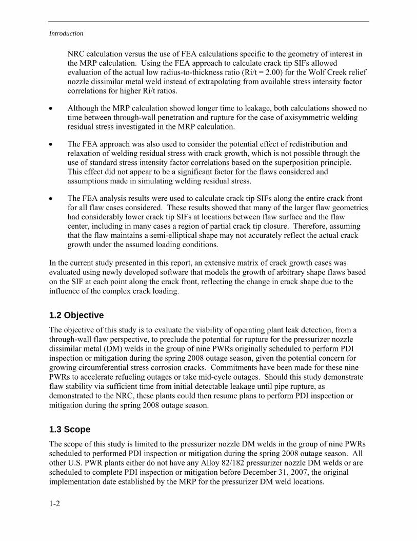
NRC calculation versus the use of FEA calculations specific to the geometry of interest in the MRP calculation. Using the FEA approach to calculate crack tip SIFs allowed evaluation of the actual low radius-to-thickness ratio (Ri/t = 2.00) for the Wolf Creek relief nozzle dissimilar metal weld instead of extrapolating from available stress intensity factor correlations for higher Ri/t ratios.

• Although the MRP calculation showed longer time to leakage, both calculations showed no time between through-wall penetration and rupture for the case of axisymmetric welding residual stress investigated in the MRP calculation.

• The FEA approach was also used to consider the potential effect of redistribution and relaxation of welding residual stress with crack growth, which is not possible through the use of standard stress intensity factor correlations based on the superposition principle. This effect did not appear to be a significant factor for the flaws considered and assumptions made in simulating welding residual stress.

• The FEA analysis results were used to calculate crack tip SIFs along the entire crack front for all flaw cases considered. These results showed that many of the larger flaw geometries had considerably lower crack tip SIFs at locations between flaw surface and the flaw center, including in many cases a region of partial crack tip closure. Therefore, assuming that the flaw maintains a semi-elliptical shape may not accurately reflect the actual crack growth under the assumed loading conditions.

In the current study presented in this report, an extensive matrix of crack growth cases was evaluated using newly developed software that models the growth of arbitrary shape flaws based on the SIF at each point along the crack front, reflecting the change in crack shape due to the influence of the complex crack loading.

1.2 Objective The objective of this study is to evaluate the viability of operating plant leak detection, from a through-wall flaw perspective, to preclude the potential for rupture for the pressurizer nozzle dissimilar metal (DM) welds in the group of nine PWRs originally scheduled to perform PDI inspection or mitigation during the spring 2008 outage season, given the potential concern for growing circumferential stress corrosion cracks. Commitments have been made for these nine PWRs to accelerate refueling outages or take mid-cycle outages. Should this study demonstrate flaw stability via sufficient time from initial detectable leakage until pipe rupture, as demonstrated to the NRC, these plants could then resume plans to perform PDI inspection or mitigation during the spring 2008 outage season.

1.3 Scope The scope of this study is limited to the pressurizer nozzle DM welds in the group of nine PWRs scheduled to performed PDI inspection or mitigation during the spring 2008 outage season. All other U.S. PWR plants either do not have any Alloy 82/182 pressurizer nozzle DM welds or are scheduled to complete PDI inspection or mitigation before December 31, 2007, the original implementation date established by the MRP for the pressurizer DM weld locations.

Introduction

1-3

The nine subject PWR plants are Braidwood 2, Comanche Peak 2, Diablo Canyon 2, Palo Verde 2, Seabrook, South Texas Project 1, V.C. Summer, Vogtle 1, and Waterford 3. Fifty-one of the total number of 53 pressurizer nozzles in these plants are within the scope of this study. The spray nozzle in one plant was PDI inspected in 2005, and as such is not included in the scope. In addition, the surge nozzle in one plant has already had weld overlay application, and as such is not included in the scope. Seven of the nine subject plants are Westinghouse design plants, and the other two are CE design plants. Figures 1-1 through 1-3 illustrate the nozzle locations and example configurations for pressurizer nozzles in Westinghouse and CE design plants. As discussed in Section 2, detailed weld-specific geometry, load, and fabrication parameters were collected for all 51 subject welds.

1.4 Approach In order to facilitate modeling of the crack shape development and in direct support of this study, Quest Reliability, LLC extended its FEACrack software to model the growth of circumferential flaws having a custom profile. In Phase I of this study, the new software tools were applied to the same basic weld geometry, piping load inputs, and welding residual stress distribution assumed in the previous MRP calculation [4]. In Phase II, an extensive crack growth sensitivity matrix was investigated to cover the geometry, load, and fabrication factors for each of the 51 subject welds, as well as the uncertainty in key modeling parameters such as those associated with welding residual stress, initial crack shape and depth, the K-dependence of the crack growth rate equation, and the effect of multiple flaw initiation sites in a single weld. Other key Phase II activities included detailed welding residual stress simulations covering the subject welds, development of a conservative crack stability calculation methodology, development of a leak rate calculation procedure using existing software tools (EPRI PICEP and NRC SQUIRT), and verification and validation studies.

1.5 Expert Panel In support of this study, EPRI assembled a panel of experts experienced in the application of fracture mechanics tools to the evaluation of stress corrosion cracking. The panel included representation of individuals not recently involved in the evaluation of PWSCC in PWR components. The panel provided detailed input into all phases of the project as the work progressed.

1.6 Report Structure

The organization of this report is described below.

1. INTRODUCTION (SECTION 1)

This introductory section provides a brief background discussion, defines the purpose and scope of this study, and outlines the approach used.

Introduction

1-4

2. PLANT INPUTS (SECTION 2)

Section 2 summarizes the extensive weld-specific dimensional, piping load, fabrication, and weld repair history inputs that were collected for the group of 51 subject pressurizer nozzles. Detailed geometry and piping load inputs were collected for each subject weld to ensure that all welds are appropriately addressed by the crack growth sensitivity matrix (Section 7) developed as part of this study. Weld-specific fabrication and weld repair data were also collected as a key input to the welding residual stress simulations addressing the subject population (Section 3). Appendix A contains more detailed information on the design and fabrication of the subject nozzles and welds.

3. WELDING RESIDUAL STRESS (SECTION 3)

Section 3 discusses the matrix of welding residual stress (WRS) simulations that were performed on the basis of the detailed design, fabrication, and weld repair information collected. Axisymmetric and non-axisymmetric weld repair WRS profiles were developed for input to the crack growth simulations under various assumptions in recognition of the uncertainty in calculation of WRS values. Section 3 also includes the results of validation work comparing a WRS simulation by the authors to stress measurements and the simulations of other organizations for a piping butt weld mockup.

4. CRACK GROWTH MODELING (SECTION 4)

Section 4 describes the new crack growth simulation methodology, including development of the new extensions to the FEACrack software and application of the new software in the Phase I calculations based on the same Wolf Creek relief nozzle inputs previously evaluated on the basis of an assumed semi-elliptical crack shape. Section 4 also includes the results of verification and validation work, including calculation convergence checks.

5. CRITICAL CRACK SIZE CALCULATIONS (SECTION 5)

Section 5 describes the development of a conservative critical crack size methodology specific to the subject nozzle-to-safe-end geometry and materials. This methodology is based on the net section collapse (NSC) equations for an arbitrary circumferential crack profile in a thin-walled pipe. As discussed in Section 5 and for the purposes of this project, normal thermal piping loads were included in the crack stability calculations, and a Z-factor approach reducing the NSC failure load was implemented in consideration of the possibility of an EPFM failure mechanism. Finally, in support of the methodology, available experimental failure data for complex cracks in materials similar to Alloy 82/182 were evaluated.

6. LEAK RATE MODELING (SECTION 6)

Section 6 describes the leak rate calculation procedure applied to the through-wall portion of the crack growth simulations using EPRI’s PICEP software. The crack opening area at the weld OD calculated in the crack growth finite-element simulations was applied directly in the PICEP leak rate calculations. NRC’s SQUIRT software was also applied in a scoping study for the purpose of comparison.

7. SENSITIVITY CASE MATRIX (SECTION 7)

Section 7 discusses the development and application of an extensive crack growth sensitivity matrix covering the geometry, load, and fabrication factors for each of the 51

Introduction

1-5

subject welds, as well as the uncertainty in key modeling parameters such as those associated with welding residual stress, initial crack shape and depth, the K-dependence of the crack growth rate equation, and the effect of multiple flaw initiation sites in a single weld. Section 7 also presents a set of evaluation criteria that was developed to guide interpretation of the matrix results. The evaluation criteria provide safety margins based on explicit consideration of leak rate detection sensitivity, plant response time, and uncertainty in the crack stability calculations.

8. SUMMARY AND CONCLUSIONS (SECTION 8)

Section 8 summarizes this study, including the main conclusions. It is concluded that all 51 subject welds are adequately covered by crack growth sensitivity cases that satisfy the evaluation criteria presented in Section 7.2.

9. REFERENCES (SECTION 9)

Section 9 lists the references cited in the main body of this report.

10. APPENDIX A: DISSIMILAR METAL BUTT WELD FABRICATION PROCESSES

Appendix A describes the detailed nozzle fabrication practices for the subject set of pressurizer nozzle welds. In addition, Appendix A includes design sketches with key dimensions for the subject welds.

11. APPENDIX B: EVALUATION OF THE EFFECTS OF SECONDARY STRESSES ON SURGE LINE CRITICAL FLAW SIZE CALCULATIONS

In support of the critical flaw size analyses described in Section 5, Appendix B describes analyses of the effects of secondary (displacement controlled) loads on critical flaw size. The evaluation included a review of test data from the NRC-sponsored Degraded Piping Program. Detailed test data from selected full scale pipe tests of relevant materials, pipe sizes, and flaw types were reviewed to determine the amount of crack plane rotation that was tolerated in the tests prior to failure. In addition, piping models were developed for the surge lines of two representative plants to evaluate the maximum capacity of the secondary loads to produce rotation at a cracked surge nozzle, relative to the rotational tolerance of a nozzle weld containing a large complex crack. The results of this study support the conclusion that the surge nozzle piping thermal loads are completely relieved prior to nozzle rupture.

12. APPENDIX C: SECONDARY STRESS STUDY—PIPE BENDING WITH A THROUGH-THICKNESS CRACK

Appendix C describes elastic and elastic-plastic finite element analyses of a pipe with an idealized through-thickness crack that were used to determine the effect on bending moment and crack driving force due to an imposed end rotation. Because of the finite amount of strain imposed by the rotation, the results show that the moment knock-down factor and crack driving force relative to the load controlled case decrease significantly as the crack length increases. These results further support the conclusions of Appendix B, and demonstrate the general tendency for relief of secondary piping loads given sufficient crack plane rotation.

Introduction

1-6

13. APPENDIX D: SCATTER IN LEAK RATE PREDICTIONS

Appendix D describes a statistical study of experimental leak rate data for through-wall cracks having an IGSCC morphology. This study shows that a multiplicative factor of 1.5 to 2.0 on the leak rate calculated using the NRC SQUIRT code describes the uncertainty in leak rate due to scatter in the test data for the IGSCC samples tested. A leak rate margin factor of 4.0 is applied in Section 7 in recognition of other sources of uncertainty in the leak rate calculation not addressed by this statistical evaluation such as the variability in the PWSCC crack morphology parameters (e.g., crack surface roughness and tortuosity) versus the PWSCC type assumptions in Section 6.

14. APPENDIX E: EVALUATION OF PRESSURIZER ALLOY 82/182 NOZZLE FAILURE PROBABILITY

Appendix E describes the methodology and results of a complementary probabilistic study. This study considered current inspection data to assess the effect of various inspection options on the probability of a nozzle failure in the time interval until all nozzles are inspected or mitigated. Appendix E concludes that there is no significant benefit, in terms of reduced nozzle failure probability, to accelerating the originally scheduled spring 2008 inspections.

Introduction

1-7

Figure 1-1 Pressurizer Nozzle Locations for Westinghouse and CE Design Plants

Example Pressurizer Surge Nozzle Example Pressurizer Safety/Relief Nozzle

Figure 1-2 Example Westinghouse Design Pressurizer Nozzles

2

6

4 3

1

7

5

3

2

3

1

Example Westinghouse Design Pressurizer Example CE Design Pressurizer

1. Surge Nozzle 2. Spray Nozzle 3. Safety/Relief Nozzle

Introduction

1-8

Figure 1-3 Example CE Design Pressurizer Safety/Relief Nozzle

2-1

2 PLANT INPUTS

This section summarizes the extensive weld-specific dimensional, piping load, fabrication, and weld repair history inputs that were collected for the group of 51 subject pressurizer nozzles. Detailed geometry and piping load inputs were collected for each subject weld to ensure that all welds are appropriately addressed by the crack growth sensitivity matrix (Section 7) developed as part of this study. Weld-specific fabrication and weld repair data were also collected as a key input to the welding residual stress simulations addressing the subject population (Section 3).

2.1 Geometry Cases

Among the nine plants covered in this report, there are a total of 51 pressurizer dissimilar metal welds of concern comprising: a) 35 safety and relief (S&R) nozzles, b) 8 surge nozzles, and c) 8 spray nozzles. Nozzle details are also included for a reference Plant J (Wolf Creek). Details of all nozzles at all plants are discussed fully in Appendix A [5,7]. The nozzle geometry information for the nozzles are summarized in Table 2-1 and Figure 2-1. The 51 nozzles may be further categorized into the following nozzle geometry cases. Note that nozzles with the same overall geometry may have been manufactured differently; see Section 2.3 for additional discussion.

2.1.1 Safety/Relief Nozzles

• Types 1a and 1b: Westinghouse design without liner, connected to 6" pipe, used at plants A, E, H, and J (Type 1a) and plant F (Type 1b).

• Types 2a and 2b: Westinghouse design with liner directly covering DM weld, connected to 6" pipe, used at plants B, C, and G.

• Type 3: CE design (no liner), connected to 6" pipe, used at plants D and I.

2.1.2 Spray Nozzles

• Type 4: Westinghouse design with liner (does not extend to most of DM weld), connected to 4" pipe, used at plants A, E, and J.

• Type 5: Westinghouse design with liner directly covering DM weld, connected to 4" pipe, used at plants B, C, and G.

• Type 6: Westinghouse design without liner, connected to 6" pipe, used at plant F.

• Type 7: CE design (no liner, sleeve not extending to DM weld), connected to 4" pipe, used at plants D and I.

Plant Inputs

2-2

2.1.3 Surge Nozzles

• Type 8: Westinghouse design, sleeve directly covers DM weld area, connected to 14" pipe. Used at plants A, B, C, E, F, G, H, and J. Note that this weld has already been mitigated at plant F.

• Type 9: CE design, DM weld machined at ID, sleeve does not extend to DM weld, connected to 12" pipe, see Section A.2.1. Used at plants D and I.

2.2 Piping Load Inputs

2.2.1 Pressure, Dead Weight, and Normal Thermal Loads

The piping loads for the 51 subject nozzle welds at the nine plants were also provided in References [5,7]. The loads are summarized in Figure 2-2 through Figure 2-6. In these figures, each point along the x-axis of the plots represents an individual nozzle weld. From left to right, the safety/relief nozzles at all plants are grouped together, followed by the spray nozzles, with the surge nozzles at the far right. The axial loads are displayed in Figure 2-2 and the bending moment loads are displayed in Figure 2-3 and Figure 2-4. Pressure and deadweight stresses (i.e., primary stresses) are displayed in Figure 2-5, and primary plus normal operating thermal stresses are displayed in Figure 2-6. As noted in Section 5, the primary plus normal operating thermal stress is used to calculate the critical flaw size.

For the purpose of showing the relative magnitudes of the membrane stress in these figures, the ASME Section XI Code definition pDo/4t where p is the pressure, Do is the outside diameter, and t is the wall thickness has been used for the pressure loading component. Because this ASME Code definition is based on the outside diameter, it conservatively captures the effect of pressure acting on the crack face. However, in the crack growth and crack stability calculations performed for the sensitivity matrix of Section 7, the end cap pressure loading is based on the inside diameter cross sectional area plus the crack area, which depends on the particular calculated crack profile. The piping load stresses presented in Section 2 are independent of any particular crack profile assumption.

2.2.2 Surge Line Thermal Stratification Effects

An additional load condition that is unique to the surge nozzles (among the nozzles considered) is thermal stratification. Thermal stratification occurs in the surge line of every operating plant, due to the temperature difference between the pressurizer and the hot leg, which are connected by the surge line. The stratification produces a piping bending load, which can affect the surge nozzle safe end region. The normal operating thermal stratification loadings existing on the piping system during steady state operation are typically not significantly different from the normal operating thermal expansion loadings without thermal stratification (and sometimes ameliorate the loadings). Therefore, normal operating thermal stratification loadings are not considered in the crack growth or critical crack size analysis. It is noted that Reference [5] includes loads under the heading “Normal Thermal Stratification”. However, recent

Plant Inputs

2-3

investigation has revealed that, in some cases, the loads listed in this table are for other, more limiting, cases and should not be considered.

The stratification loads for some plants become significant during heat-up and cooldown of the plant, when the pressurizer and hot leg temperature differential may be larger. The limiting thermal loads for all surge nozzles are reported in Reference [7]; these loads are the entire maximum thermal load including all other effects, such as piping expansion. This table also notes that sometimes the limiting thermal load occurs during the normal operating condition (i.e., no thermal stratification). A series of comparison figures are included in this report comparing the normal and limiting thermal loads. In each figure, the primary (pressure plus dead weight) plus normal thermal loads are compared to the primary plus limiting thermal loads. Figure 2-7 compares the axial (membrane, Pm) stress between the two conditions at all plants; Figure 2-8 compares the bending (Pb) stress between the two conditions at all plants; and Figure 2-9 compares the combined membrane plus bending stress (Pm+Pb) between the two conditions at all plants. The ratio between the primary plus normal thermal and primary plus limiting thermal conditions for the Pm, Pb, and Pm+Pb stresses are compared in Figure 2-10.

As shown in Figure 2-10, when the normal and limiting stresses differ, they differ only in bending stress. Additionally, the primary plus normal thermal stress at any plant is no less than 45% of the corresponding primary plus limiting thermal stress, and, in many cases, it is closer to 100% of the primary plus limiting thermal stress. Given that Appendix B and Appendix C include separate calculations detailing how thermal bending loads would be expected to significantly relax in the presence of a large circumferential flaw, calculation of the critical flaw size using primary plus normal thermal loads is considered appropriate.

2.3 Weld Fabrication

The fabrication information for the 51 subject nozzle welds is summarized in Table 2-1. As described in Appendix A, the fabrication process for all nozzles falls under one of two general classifications identified in Table A-1, “Back-Weld” or “Machined.” All the nozzles at a given plant share the same general fabrication process; i.e., no plant has some nozzles fabricated per the “Back-Weld” classification and others per “Machined.” The two processes are summarized as follows; further detail is provided in Appendix A [5,7].

2.3.1 “Back-Weld” Process

The “Back-Weld” process uses U-groove type design with a specified back-weld; i.e., a weld on the “back” side (in this case the ID side) of the weld joint. In this design, the two sides of the weld meet at an initial land that is 0.060 inches thick. Initial passes are applied to melt through the land and join the two sections. The weld is performed from ID to OD from the outside of the weld preparation. Once the initial weld is complete, the inside surface at the land joint is dye penetrant inspected, and the ID is ground until no separation is observed between the two sides of the land. While the design of the initial passes was intended to melt through and join the land, it is possible that the land region was ground in a fully circumferential manner to the approximate thickness of the land. Any material removed by grinding was filled in with a back-

Plant Inputs

2-4

weld out to the ID surface. The complete weld was then radiographed, and repairs were made as necessary.

In the case of the surge nozzle, an additional step is applied following the radiograph/repair process. Following this step, a weld cladding layer (referred to as a fill-in weld) was deposited over the ID of the weld region to create a flat mating surface for the thermal sleeve. At its thickest point, the fill-in weld is about 0.3 inches thick. The fill-in weld layer was not radiographed.

Plants with nozzles manufactured using the “back-weld” process are A, B, C, F, G, and J.

2.3.2 “Machined” Process

The nozzle weld preparation design for the plants that use the “Machined” process differs from the “Back-Weld” process in that the ID of the weld prep was smaller than the desired finished ID. The weld is completed from ID to OD. After the weld is complete, the inside surface material is machined away to the desired finished dimension. Typically, in this type of joint, the initial root passes are machined away as part of the final machining to the finished ID. Surge nozzles fabricated using the “Machined” process do not have a fill-in weld layer.

Plants with nozzles manufactured using the “Machined” process are E and H (Westinghouse design) and D and I (CE design). As noted in Section A.5, the original design for plants E and H was to use a “Back-Weld” process; the change was made during the fabrication of the pressurizer and is not reflected in the design drawings shown in Appendix A.

2.4 Weld Repair History

The weld repair history for the 51 subject nozzle welds is noted in Table 2-1, and is described in greater detail in Table 2-2 [5,6,8]. Table 2-2 shows, when available, the number, depth, and length of the repairs for each weld.

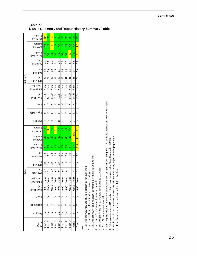
Plant Inputs

2-5

Table 2-1 Nozzle Geometry and Repair History Summary Table

Design #

Piping NPS

Liner?

Land Thick (in.)

Fill-In Weld Thick. (in.)

DM Weld t (in.)

DM Weld Ri/t

Weld Sep. (in.)

Butter Weld Repairs

ID Weld Repairs

OD Weld Repairs

Design #

Piping NPS

Liner?

Land Thick (in.)

Fill-In Weld Thick. (in.)

DM Weld t (in.)

DM Weld Ri/t

Weld Sep. (in.)

Butter Weld Repairs

ID Weld Repairs

OD Weld Repairs

Plan

t A1a

6"N

0.06

Non

e1.

292.

02.

2N

RN

RN

R1a

6"N

0.06

Non

e1.

292.

02.

2N

RN

RR

4Pl

ant E

1a6"

NM

ach

Non

e1.

292.

02.

2N

RN

RR

1a6"

NM

ach

Non

e1.

292.

02.

2N

RN

RN

RPl

ant H

1a6"

NM

ach

Non

e1.

292.

02.

2N

RN

RN

R1a

6"N

Mac

hN

one

1.29

2.0

2.2

NR

RR

Plan

t B2a

6"Y

0.06

Non

e1.

072.

62.

6N

RN

RR

12a

6"Y

0.06

Non

e1.

072.

62.

6N

RN

RN

RPl

ant G

2a6"

Y0.

06N

one

1.07

2.6

2.6

NR

NR

NR

2a6"

Y0.

06N

one

1.07

2.6

2.6

NR

NR

NR

Plan

t C2b

6"Y

0.06

Non

e1.

072.

62.

3N

RN

RN

R2b

6"Y

0.06

Non

e1.

072.

62.

3N

RN

RN

RPl

ant F

1b6"

N0.

06N

one

1.41

1.8

3.3

NR

NR

NR

1b6"

N0.

06N

one

1.41

1.8

3.3

NR

NR

NR

Plan

t D3

6"N

Mac

hN

one

1.41

1.8

6.8

NR

NR

NR

36"

NM

ach

Non

e1.

411.

86.

8R

NR

NR

Plan

t I3

6"N

Mac

hN

one

1.41

1.8

6.8

NR

36"

NM

ach

Non

e1.

411.

86.

8N

RN

RN

RPl

ant J

1a6"

N0.

06N

one

1.29

2.0

2.2

Rx5

R1

R1

1a6"

N0.

06N

one

1.29

2.0

2.2

RR

2N

R

Not

es:

1. F

or D

esig

ns #

2a, #

2b, a

nd #

5, li

ner d

irect

ly c

over

s DM

wel

d.2.

For

Des

ign

#4, l

iner

doe

s not

ext

end

to m

ost o

f DM

wel

d.3.

For

Des

igns

#4,

#5,

and

#6,

slee

ve c

over

s but

doe

s not

con

tact

DM

wel

d.4.

For

Des

ign

#8, s

leev

e di

rect

ly c

over

s DM

wel

d.5.

For

Des

igns

#7

and

#9, s

leev

e do

es n

ot e

xten

d to

DM

wel

d.6.

NR

= N

o w

eld

repa

irs re

porte

d7.

Rn

= R

epai

rs re

porte

d (n

indi

cate

s num

ber o

f def

ect o

r rep

aire

d ar

eas i

f rep

orte

d; "

x" in

dica

tes r

epea

t wel

d re

pair

oper

atio

ns)

8. A

ll pr

essu

rizer

noz

zle

DM

wel

ds in

Pla

nt H

are

repo

rted

to b

e A

lloy

82, n

ot A

lloy

82/1

82.

9. M

ach

= In

itial

land

thic

knes

s of 0

.09"

to 0

.10"

mac

hine

d aw

ay a

s par

t of w

eld

prep

des

ign.

10.

Plan

t I c

appe

d re

lief n

ozzl

e lis

ted

unde

r "R

elie

f" h

eadi

ng.

Safe

ty A

Plan

tC

ode

Rel

ief

Rx2

Plant Inputs

2-6

Table 2-1 (cont’d) Nozzle Geometry and Repair History Summary Table

Design #

Piping NPS

Liner?

Land Thick (in.)

Fill-In Weld Thick. (in.)

DM Weld t (in.)

DM Weld Ri/t

Weld Sep. (in.)

Butter Weld Repairs

ID Weld Repairs

OD Weld Repairs

Design #

Piping NPS

Liner?

Land Thick (in.)

Fill-In Weld Thick. (in.)

DM Weld t (in.)

DM Weld Ri/t

Weld Sep. (in.)

Butter Weld Repairs

ID Weld Repairs

OD Weld Repairs

Plan

t A1a

6"N

0.06

Non

e1.

292.

02.

2N

RR

1N

R1a

6"N

0.06

Non

e1.

292.

02.

2N

RN

RN

RPl

ant E

1a6"

NM

ach

Non

e1.

292.

02.

2N

RN

RN

R1a

6"N

Mac

hN

one

1.29

2.0

2.2

NR

RN

RPl

ant H

1a6"

NM

ach

Non

e1.

292.

02.

2N

RN

RN

R1a

6"N

Mac

hN

one

1.29

2.0

2.2

NR

NR

NR

Plan

t B2a

6"Y

0.06

Non

e1.

072.

62.

6N

RN

RN

R2a

6"Y

0.06

Non

e1.

072.

62.

6N

RN

RN

RPl

ant G

2a6"

Y0.

06N

one

1.07

2.6

2.6

NR

NR

NR

2a6"

Y0.

06N

one

1.07

2.6

2.6

NR

NR

NR

Plan

t C2b

6"Y

0.06

Non

e1.

072.

62.

3N

RN

RN

R2b

6"Y

0.06

Non

e1.

072.

62.

3N

RN

RN

RPl

ant F

1b6"

N0.

06N

one

1.41

1.8

3.3

NR

NR

NR

1b6"

N0.

06N

one

1.41

1.8

3.3

NR

NR

NR

Plan

t D3

6"N

Mac

hN

one

1.41

1.8

6.8

NR

NR

NR

36"

NM

ach

Non

e1.

411.

86.

8N

RN

RN

RPl

ant I

36"

NM

ach

Non

e1.

411.

86.

8N

RN

RN

RPl

ant J

1a6"

N0.

06N

one

1.29

2.0

2.2

NR

R6x

2N

R1a

6"N

0.06

Non

e1.

292.

02.

2N

RN

RN

R

Not

es:

1. F

or D

esig

ns #

2a, #

2b, a

nd #

5, li

ner d

irect

ly c

over

s DM

wel

d.2.

For

Des

ign

#4, l

iner

doe

s not

ext

end

to m

ost o

f DM

wel

d.3.

For

Des

igns

#4,

#5,

and

#6,

slee

ve c

over

s but

doe

s not

con

tact

DM

wel

d.4.

For

Des

ign

#8, s

leev

e di

rect

ly c

over

s DM

wel

d.5.

For

Des

igns

#7

and

#9, s

leev

e do

es n

ot e

xten

d to

DM

wel

d.6.

NR

= N

o w

eld

repa

irs re

porte

d7.

Rn

= R

epai

rs re

porte

d (n

indi

cate

s num

ber o

f def

ect o

r rep

aire

d ar

eas i

f rep

orte

d; "

x" in

dica

tes r

epea

t wel

d re

pair

oper

atio

ns)

8. A

ll pr

essu

rizer

noz

zle

DM

wel

ds in

Pla

nt H

are

repo

rted

to b

e A

lloy

82, n

ot A

lloy

82/1

82.

9. M

ach

= In

itial

land

thic

knes

s of 0

.09"

to 0

.10"

mac

hine

d aw

ay a

s par

t of w

eld

prep

des

ign.

10.

Plan

t I c

appe

d re

lief n

ozzl

e lis

ted

unde

r "R

elie

f" h

eadi

ng.

No

Safe

ty C

Plan

tC

ode

Safe

ty B

Safe

ty C

Plant Inputs

2-7

Table 2-1 (cont’d) Nozzle Geometry and Repair History Summary Table

Design #

Piping NPS

Liner?

Land Thick (in.)

Fill-In Weld Thick. (in.)

DM Weld t (in.)

DM Weld Ri/t

Weld Sep. (in.)

Butter Weld Repairs

ID Weld Repairs

OD Weld Repairs

Design #

Piping NPS

Liner?

Land Thick (in.)

Fill-In Weld Thick. (in.)

DM Weld t (in.)

DM Weld Ri/t

Weld Sep. (in.)

Butter Weld Repairs

ID Weld Repairs

OD Weld Repairs

Plan

t A1a

6"N

0.06

Non

e1.

292.

02.

2N

RR

1N

R1a

6"N

0.06

Non

e1.

292.

02.

2N

RN

RN

RPl

ant E

1a6"

NM

ach

Non

e1.

292.

02.

2N

RN

RN

R1a

6"N

Mac

hN

one

1.29

2.0

2.2

NR

RN

RPl

ant H

1a6"

NM

ach

Non

e1.

292.

02.

2N

RN

RN

R1a

6"N

Mac

hN

one

1.29

2.0

2.2

NR

NR

NR

Plan

t B2a

6"Y

0.06

Non

e1.

072.

62.

6N

RN

RN

R2a

6"Y

0.06

Non

e1.

072.

62.

6N

RN

RN

RPl

ant G

2a6"

Y0.

06N

one

1.07

2.6

2.6

NR

NR

NR

2a6"

Y0.

06N

one

1.07

2.6

2.6

NR

NR

NR

Plan

t C2b

6"Y

0.06

Non

e1.

072.

62.

3N

RN

RN

R2b

6"Y

0.06

Non

e1.

072.

62.

3N

RN

RN

RPl

ant F

1b6"

N0.

06N

one

1.41

1.8

3.3

NR

NR

NR

1b6"

N0.

06N

one

1.41

1.8

3.3

NR

NR

NR

Plan

t D3

6"N

Mac

hN

one

1.41

1.8

6.8

NR

NR

NR

36"

NM

ach

Non

e1.

411.

86.

8N

RN

RN

RPl

ant I

36"

NM

ach

Non

e1.

411.

86.

8N

RN

RN

RPl

ant J

1a6"

N0.

06N

one

1.29

2.0

2.2

NR

R6x

2N

R1a

6"N

0.06

Non

e1.

292.

02.

2N

RN

RN

R

Not

es:

1. F

or D

esig

ns #

2a, #

2b, a

nd #

5, li

ner d

irect

ly c

over

s DM

wel

d.2.

For

Des

ign

#4, l

iner

doe

s not

ext

end

to m

ost o

f DM

wel

d.3.

For

Des

igns

#4,

#5,

and

#6,

slee

ve c

over

s but

doe

s not

con

tact

DM

wel

d.4.

For

Des

ign

#8, s

leev

e di

rect

ly c

over

s DM

wel

d.5.

For

Des

igns

#7

and

#9, s

leev

e do

es n

ot e

xten

d to

DM

wel

d.6.

NR

= N

o w

eld

repa

irs re

porte

d7.

Rn

= R

epai

rs re

porte

d (n

indi

cate

s num

ber o

f def

ect o

r rep

aire

d ar

eas i

f rep

orte

d; "

x" in

dica

tes r

epea

t wel

d re

pair

oper

atio

ns)

8. A

ll pr

essu

rizer

noz

zle

DM

wel

ds in

Pla

nt H

are

repo

rted

to b

e A

lloy

82, n

ot A

lloy

82/1

82.

9. M

ach

= In

itial

land

thic

knes

s of 0

.09"

to 0

.10"

mac

hine

d aw

ay a

s par

t of w

eld

prep

des

ign.

10.

Plan

t I c

appe

d re

lief n

ozzl

e lis

ted

unde

r "R

elie

f" h

eadi

ng.

No

Safe

ty C

Plan

tC

ode

Safe

ty B

Safe

ty C

Plant Inputs

2-8

Table 2-2 Weld Repair Summary Table

Tabl

eLi

nePl

ant

Cod

eN

ozzl

eTy

peN

ozzl

eC

ount

Des

ign

#B

utte

ring

or W

eld

Leng

t h(in

.)D

epth

(in.)

Leng

th(in

.)D

epth

(in.)

Leng

th(in

.)D

epth

(in.)

Leng

th(in

.)D

epth

(in.)

Leng

t h(in

.)D

epth

(in.)

Leng

th(in

.)D

epth

(in.)

1A

Safe

ty A

11a

wel

dO

DN

/AN

/A4

N/A

~1/2

N/A

~1/2

N/A

~1/2

N/A

~1/2

2A

Safe

ty B

21a

wel

dID

N/A

N/A

11/

25/

83

ER

elie

f3

1aw

eld

OD

N/A

NN

/AN

/AN

/A4

ESa

fety

C4

1aw

eld

ID<2

2%N

/AN

N/A

N/A

N/A

5ID

82Y

N/A

N/A

N/A

6O

D82

YN

/AN

/AN

/A7

BR

elie

f6

2aw

eld

OD

182

N/A

10.

50.

375

8D

Safe

ty A

73

butte

rN

/AN

/AY

N/A

N/A

N/A

9I

Rel

ief

83

wel

dID

+OD

82/1

82N

8N

/AN

/A10

butte

rID

82Y

N/A

N/A

~0.3

11w

eld

OD

N/A

NN

/AN

/AN

/A12

FSp

ray

106

butte

rN

/A82

YN

/AN

/AN

/A13

IDN

/AN

/A5

1.5

5/16

3.75

0.5

23/

162.

55/

162

5/16

14O

DN

/AN

/A3

2.5

0.5

20.

51

3/16

15E

Surg

e12

8w

eld

ID<1

0%82

N3

N/A

N/A

N/A

N/A

N/A

N/A

16bu

tter

N/A

82Y

1N

/AN

/A17

OD

182

N/A

21.

750.

875

1.5

118

ID18

2N

/A1

1.0

0.62

519

ID18

2N

/A1

40.

7520

ISu

rge

149

wel

dID

+OD

82/1

82N

4N

/AN

/AW

C1

N/A

82/1

82Y

N/A

N/A

N/A

WC

2ID

+OD

82Y

21/

27/

16ID

17/

16O

DW

C3

OD

182

Y1

13/

4W

C4

ID82

Y3

3/4

3/4

2-1/

43/

41/

23/

4W

C5

OD

182

Y3

13/

42-

1/4

3/4

1/2

3/4

WC

6O

D82

N/A

11-

1/4

1/2

WC

7ID

82N

/A1

1/2

1/2

WC

8bu

tter

N/A

182

YN

/AN

/A1/

8W

C9

wel

dID

82N

/A2

1-1/

411

/32

7/8

11/3

2W

C10

82N

/A6

2-1/

23/

41

1/2

1-1/

21/

21

1/2

2-1/

23/

42-

1/2

3/4

WC

1182

N/A

61-

1/2

1/2

1-1/

41

3/4

7/8

1-1/

23/

81

1-1/

161/

21/

2W

C12

JSp

ray

WC

44

butte

rlip

/bon

dlin

e82

YN

/AN

/AN

/AW

C13

butte

rO

D18

2Y

27/

89/

161-

1/8

1W

C14

wel

dID

82Y

11

7/16

Not

es:

1. F

or D

esig

ns #

2a, #

2b, a

nd #

5, li

ner d

irect

ly c

over

s DM

wel

d.2.

For

Des

ign

#4, l

iner

doe

s not

ext

end

to m

ost o

f DM

wel

d.3.

For

Des

igns

#4,

#5,

and

#6,

slee

ve c

over

s but

doe

s not

con

tact

DM

wel

d.4.

For

Des

ign

#8, s

leev

e di

rect

ly c

over

s DM

wel

d.5.

N/A

= In

form

atio

n no

t ava

ilabl

e

ID/O

D(% circ

.)

JSa

fety

BW

C3

1aw

eld

ID

butte

r

JSa

fety

A1a

JSu

rge

8

WC

2

WC

5

wel

d

JR

elie

f1a

WC

1

wel

d

wel

dB

Surg

e8

11 13

ESp

ray

4

ASu

rge

8

9

Safe

ty A

H1a

wel

d5

PWH

Taf

ter

Re p

air?

Allo

y82

or

182

# D

efec

tor

Rep

air

Are

as

Def

ect/R

epai

rA

rea

#6D

efec

t/Rep

air

Are

a #4

Def

ect/R

epai

rA

rea

#5D

efec

t/Rep

air

Are

a #1

Def

ect/R

epai

rA

rea

#2D

efec

t/Rep

air

Are

a #3

Plant Inputs

2-9

Figure 2-1 Nominal Basic Design Dimensions for Each Subject Weld

0246810121401 A - Re (7.75x5.17)

02 A - SA (7.75x5.17)

03 A - SB (7.75x5.17)

04 A - SC (7.75x5.17)

05 E - Re (7.75x5.17)

06 E - SA (7.75x5.17)

07 E - SB (7.75x5.17)

08 E - SC (7.75x5.17)

09 H - Re (7.75x5.17)

10 H - SA (7.75x5.17)

11 H - SB (7.75x5.17)

12 H - SC (7.75x5.17)

WC1 J - Re (7.75x5.17)

WC1a J - Re/Sa (7.75x5.17)

WC2 J - SA (7.75x5.17)

WC3 J - SB (7.75x5.17)

WC4 J - SC (7.75x5.17)

13 F - Re (8x5.19)

14 F - SA (8x5.19)

15 F - SB (8x5.19)

16 F - SC (8x5.19)

17 B - Re (7.75x5.62)

18 B - SA (7.75x5.62)

19 B - SB (7.75x5.62)

20 B - SC (7.75x5.62)

21 G - Re (7.75x5.62)

22 G - SA (7.75x5.62)

23 G - SB (7.75x5.62)

24 G - SC (7.75x5.62)

25 C - Re (7.75x5.62)

26 C - SA (7.75x5.62)

27 C - SB (7.75x5.62)

28 C - SC (7.75x5.62)

29 D - Re (8x5.19)

30 D - SA (8x5.19)

31 D - SB (8x5.19)

32 D - SC (8x5.19)

33 I - Re (8x5.188)

34 I - SA (8x5.188)

35 I - SB (8x5.188)

36 A - Sp (5.81x4.01)

37 E - Sp (5.81x4.01)

WC5 J - Sp (5.81x4.01)

38 B - Sp (5.81x4.25)

39 G - Sp (5.81x4.25)

40 C - Sp (5.81x4.25)

41 F - Sp (8x5.695)

42 D - Sp (5.188x3.062)

43 I - Sp (5.188x3.25)

44 A - Su (15x11.844)

45 E - Su (15x11.844)

46 H - Su (15x11.844)

WC6 J - Su (15x11.844)

47 B - Su (15x11.844)

48 G - Su (15x11.844)

49 C - Su (15x11.875)

50 D - Su (13.063x10.125)

51 I - Su (13.063x10.125)

ID (i

n)O

D (i

n)t (

in)

ID/t

Plant Inputs

2-10

Figure 2-2 Nominal Axial Piping Loads (Not Including Endcap Pressure Load)

-15-55152535

01 A - Re (7.75x5.17)

02 A - SA (7.75x5.17)

03 A - SB (7.75x5.17)

04 A - SC (7.75x5.17)

05 E - Re (7.75x5.17)

06 E - SA (7.75x5.17)

07 E - SB (7.75x5.17)

08 E - SC (7.75x5.17)

09 H - Re (7.75x5.17)

10 H - SA (7.75x5.17)

11 H - SB (7.75x5.17)

12 H - SC (7.75x5.17)

WC1 J - Re (7.75x5.17)

WC1a J - Re/Sa (7.75x5.17)

WC2 J - SA (7.75x5.17)

WC3 J - SB (7.75x5.17)

WC4 J - SC (7.75x5.17)

13 F - Re (8x5.19)

14 F - SA (8x5.19)

15 F - SB (8x5.19)

16 F - SC (8x5.19)

17 B - Re (7.75x5.62)

18 B - SA (7.75x5.62)

19 B - SB (7.75x5.62)

20 B - SC (7.75x5.62)

21 G - Re (7.75x5.62)

22 G - SA (7.75x5.62)

23 G - SB (7.75x5.62)

24 G - SC (7.75x5.62)

25 C - Re (7.75x5.62)

26 C - SA (7.75x5.62)

27 C - SB (7.75x5.62)

28 C - SC (7.75x5.62)

29 D - Re (8x5.19)

30 D - SA (8x5.19)

31 D - SB (8x5.19)

32 D - SC (8x5.19)

33 I - Re (8x5.188)

34 I - SA (8x5.188)

35 I - SB (8x5.188)

36 A - Sp (5.81x4.01)

37 E - Sp (5.81x4.01)

WC5 J - Sp (5.81x4.01)

38 B - Sp (5.81x4.25)

39 G - Sp (5.81x4.25)

40 C - Sp (5.81x4.25)

41 F - Sp (8x5.695)

42 D - Sp (5.188x3.062)

43 I - Sp (5.188x3.25)

44 A - Su (15x11.844)

45 E - Su (15x11.844)

46 H - Su (15x11.844)

WC6 J - Su (15x11.844)

47 B - Su (15x11.844)

48 G - Su (15x11.844)

49 C - Su (15x11.875)

50 D - Su (13.063x10.125)

51 I - Su (13.063x10.125)

Faxial (kips)

DW

DW

+SS

ED

W+T

DW

+T+S

SE

DW

+T+S

trat

DW

+T+S

trat+

SSE

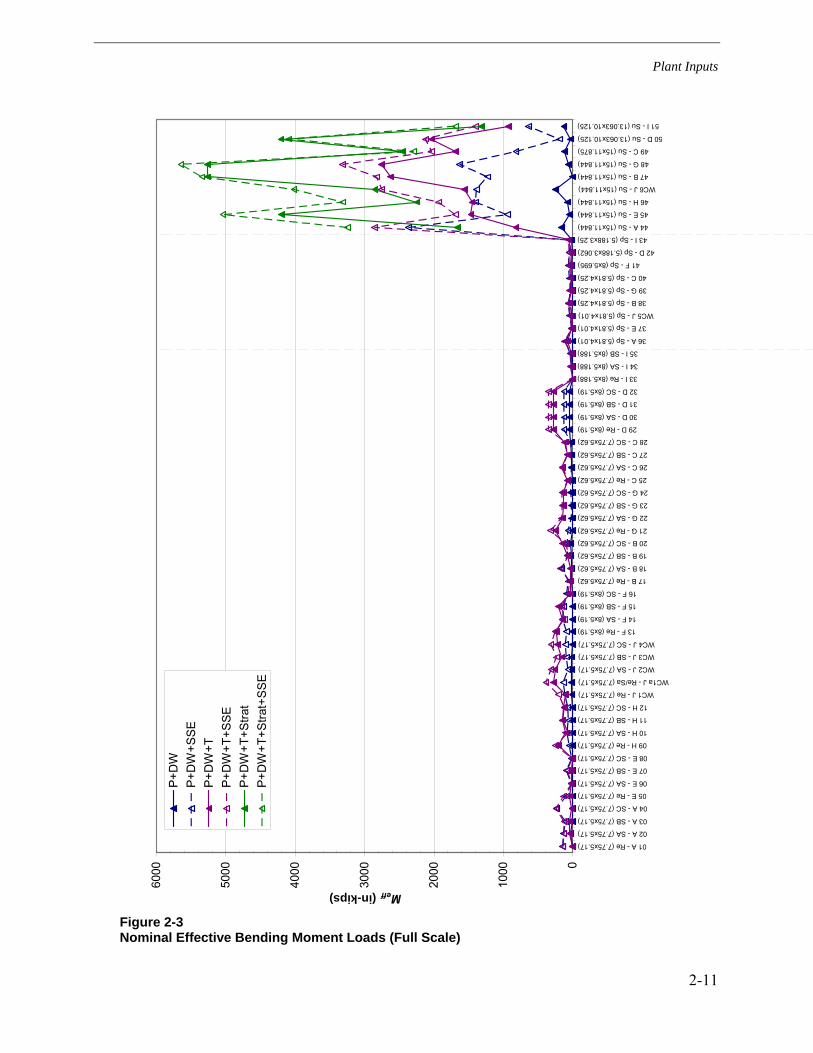
Plant Inputs

2-11

Figure 2-3 Nominal Effective Bending Moment Loads (Full Scale)

0

1000

2000

3000

4000

5000

6000

01 A - Re (7.75x5.17)

02 A - SA (7.75x5.17)

03 A - SB (7.75x5.17)

04 A - SC (7.75x5.17)

05 E - Re (7.75x5.17)

06 E - SA (7.75x5.17)

07 E - SB (7.75x5.17)

08 E - SC (7.75x5.17)

09 H - Re (7.75x5.17)

10 H - SA (7.75x5.17)

11 H - SB (7.75x5.17)

12 H - SC (7.75x5.17)

WC1 J - Re (7.75x5.17)

WC1a J - Re/Sa (7.75x5.17)

WC2 J - SA (7.75x5.17)

WC3 J - SB (7.75x5.17)

WC4 J - SC (7.75x5.17)

13 F - Re (8x5.19)

14 F - SA (8x5.19)

15 F - SB (8x5.19)

16 F - SC (8x5.19)

17 B - Re (7.75x5.62)

18 B - SA (7.75x5.62)

19 B - SB (7.75x5.62)

20 B - SC (7.75x5.62)

21 G - Re (7.75x5.62)

22 G - SA (7.75x5.62)

23 G - SB (7.75x5.62)

24 G - SC (7.75x5.62)

25 C - Re (7.75x5.62)

26 C - SA (7.75x5.62)

27 C - SB (7.75x5.62)

28 C - SC (7.75x5.62)

29 D - Re (8x5.19)

30 D - SA (8x5.19)

31 D - SB (8x5.19)

32 D - SC (8x5.19)

33 I - Re (8x5.188)

34 I - SA (8x5.188)

35 I - SB (8x5.188)

36 A - Sp (5.81x4.01)

37 E - Sp (5.81x4.01)

WC5 J - Sp (5.81x4.01)

38 B - Sp (5.81x4.25)

39 G - Sp (5.81x4.25)

40 C - Sp (5.81x4.25)

41 F - Sp (8x5.695)

42 D - Sp (5.188x3.062)

43 I - Sp (5.188x3.25)

44 A - Su (15x11.844)

45 E - Su (15x11.844)

46 H - Su (15x11.844)

WC6 J - Su (15x11.844)

47 B - Su (15x11.844)

48 G - Su (15x11.844)

49 C - Su (15x11.875)

50 D - Su (13.063x10.125)

51 I - Su (13.063x10.125)

Meff (in-kips)

00.1

0.2

0.3

0.4

0.5

0.6

0.7

0.8

0.9

1

0.00

0.75

1.50

2.25

3.00

3.75

4.50

5.25

6.00

6.75

7.50

8.25

9.00

9.75

10.50

11.25

12.00

12.75

13.50

14.25

15.00

15.75

16.50

17.25

18.00

18.75

19.50

20.25

21.00

21.75

22.50

23.25

24.00

24.75

25.50

26.25

27.00

27.75

28.50

29.25

30.00

30.75

31.50

32.25

33.00

33.75

34.50

35.25

36.00

36.75

37.50

38.25

39.00

39.75

40.50

41.25

42.00

42.75

43.50

44.25

45.00

45.75

46.50

47.25

48.00

48.75

49.50

50.25

51.00

51.75

52.50

53.25

54.00

54.75

55.50

56.25

57.00

57.75

58.50

59.25

60.00

P+D

WP

+DW

+SS

EP

+DW

+TP

+DW

+T+S

SEP

+DW

+T+S

trat

P+D

W+T

+Stra

t+S

SE

Plant Inputs

2-12

Figure 2-4 Nominal Effective Bending Moment Loads (Partial Scale)

0

100

200

300

400

500

600

700

800

01 A - Re (7.75x5.17)

02 A - SA (7.75x5.17)

03 A - SB (7.75x5.17)

04 A - SC (7.75x5.17)

05 E - Re (7.75x5.17)

06 E - SA (7.75x5.17)

07 E - SB (7.75x5.17)

08 E - SC (7.75x5.17)

09 H - Re (7.75x5.17)

10 H - SA (7.75x5.17)

11 H - SB (7.75x5.17)

12 H - SC (7.75x5.17)

WC1 J - Re (7.75x5.17)

WC1a J - Re/Sa (7.75x5.17)

WC2 J - SA (7.75x5.17)

WC3 J - SB (7.75x5.17)

WC4 J - SC (7.75x5.17)

13 F - Re (8x5.19)

14 F - SA (8x5.19)

15 F - SB (8x5.19)

16 F - SC (8x5.19)

17 B - Re (7.75x5.62)

18 B - SA (7.75x5.62)

19 B - SB (7.75x5.62)

20 B - SC (7.75x5.62)

21 G - Re (7.75x5.62)

22 G - SA (7.75x5.62)

23 G - SB (7.75x5.62)

24 G - SC (7.75x5.62)

25 C - Re (7.75x5.62)

26 C - SA (7.75x5.62)

27 C - SB (7.75x5.62)

28 C - SC (7.75x5.62)

29 D - Re (8x5.19)

30 D - SA (8x5.19)

31 D - SB (8x5.19)

32 D - SC (8x5.19)

33 I - Re (8x5.188)

34 I - SA (8x5.188)

35 I - SB (8x5.188)

36 A - Sp (5.81x4.01)

37 E - Sp (5.81x4.01)

WC5 J - Sp (5.81x4.01)

38 B - Sp (5.81x4.25)

39 G - Sp (5.81x4.25)

40 C - Sp (5.81x4.25)

41 F - Sp (8x5.695)

42 D - Sp (5.188x3.062)

43 I - Sp (5.188x3.25)

44 A - Su (15x11.844)

45 E - Su (15x11.844)

46 H - Su (15x11.844)

WC6 J - Su (15x11.844)

47 B - Su (15x11.844)

48 G - Su (15x11.844)

49 C - Su (15x11.875)

50 D - Su (13.063x10.125)

51 I - Su (13.063x10.125)

Meff (in-kips)

00.1

0.2

0.3

0.4

0.5

0.6

0.7

0.8

0.9

1

0.00

0.75

1.50

2.25

3.00

3.75

4.50

5.25

6.00

6.75

7.50

8.25

9.00

9.75

10.50

11.25

12.00

12.75

13.50

14.25

15.00

15.75

16.50

17.25

18.00

18.75

19.50

20.25

21.00

21.75

22.50

23.25

24.00

24.75

25.50

26.25

27.00

27.75

28.50

29.25

30.00

30.75

31.50

32.25

33.00

33.75

34.50

35.25

36.00

36.75

37.50

38.25

39.00

39.75

40.50

41.25

42.00

42.75

43.50

44.25

45.00

45.75

46.50

47.25

48.00

48.75

49.50

50.25

51.00

51.75

52.50

53.25

54.00

54.75

55.50

56.25

57.00

57.75

58.50

59.25

60.00

P+D

WP

+DW

+SS

EP

+DW

+TP

+DW

+T+S

SEP

+DW

+T+S

trat

P+D

W+T

+Stra

t+S

SE

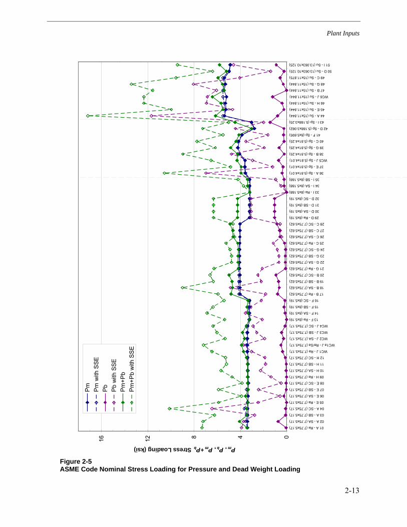
Plant Inputs

2-13

Figure 2-5 ASME Code Nominal Stress Loading for Pressure and Dead Weight Loading

048121601 A - Re (7.75x5.17)

02 A - SA (7.75x5.17)

03 A - SB (7.75x5.17)

04 A - SC (7.75x5.17)

05 E - Re (7.75x5.17)

06 E - SA (7.75x5.17)

07 E - SB (7.75x5.17)

08 E - SC (7.75x5.17)

09 H - Re (7.75x5.17)

10 H - SA (7.75x5.17)

11 H - SB (7.75x5.17)

12 H - SC (7.75x5.17)

WC1 J - Re (7.75x5.17)

WC1a J - Re/Sa (7.75x5.17)

WC2 J - SA (7.75x5.17)

WC3 J - SB (7.75x5.17)

WC4 J - SC (7.75x5.17)

13 F - Re (8x5.19)

14 F - SA (8x5.19)

15 F - SB (8x5.19)

16 F - SC (8x5.19)

17 B - Re (7.75x5.62)

18 B - SA (7.75x5.62)

19 B - SB (7.75x5.62)

20 B - SC (7.75x5.62)

21 G - Re (7.75x5.62)

22 G - SA (7.75x5.62)

23 G - SB (7.75x5.62)

24 G - SC (7.75x5.62)

25 C - Re (7.75x5.62)

26 C - SA (7.75x5.62)

27 C - SB (7.75x5.62)

28 C - SC (7.75x5.62)

29 D - Re (8x5.19)

30 D - SA (8x5.19)

31 D - SB (8x5.19)

32 D - SC (8x5.19)

33 I - Re (8x5.188)

34 I - SA (8x5.188)

35 I - SB (8x5.188)

36 A - Sp (5.81x4.01)

37 E - Sp (5.81x4.01)

WC5 J - Sp (5.81x4.01)

38 B - Sp (5.81x4.25)

39 G - Sp (5.81x4.25)

40 C - Sp (5.81x4.25)

41 F - Sp (8x5.695)

42 D - Sp (5.188x3.062)

43 I - Sp (5.188x3.25)

44 A - Su (15x11.844)

45 E - Su (15x11.844)

46 H - Su (15x11.844)

WC6 J - Su (15x11.844)

47 B - Su (15x11.844)

48 G - Su (15x11.844)

49 C - Su (15x11.875)

50 D - Su (13.063x10.125)

51 I - Su (13.063x10.125)

Pm, Pb, Pm+Pb Stress Loading (ksi)

00.1

0.2

0.3

0.4

0.5

0.6

0.7

0.8

0.9

1

0.00

0.75

1.50

2.25

3.00

3.75

4.50

5.25

6.00

6.75

7.50

8.25

9.00

9.75

10.50

11.25

12.00

12.75

13.50

14.25

15.00

15.75

16.50

17.25

18.00

18.75

19.50

20.25

21.00

21.75

22.50

23.25

24.00

24.75

25.50

26.25

27.00

27.75

28.50

29.25

30.00

30.75

31.50

32.25

33.00

33.75

34.50

35.25

36.00

36.75

37.50

38.25

39.00

39.75

40.50

41.25

42.00

42.75

43.50

44.25

45.00

45.75

46.50

47.25

48.00

48.75

49.50

50.25

51.00

51.75

52.50

53.25

54.00

54.75

55.50

56.25

57.00

57.75

58.50

59.25

60.00

Pm

Pm

with

SSE

Pb

Pb

with

SS

EP

m+P

bP

m+P

b w

ith S

SE

Plant Inputs

2-14

Figure 2-6 ASME Code Nominal Stress Loading for Pressure, Dead Weight, and Normal Thermal Loading

0510152001 A - Re (7.75x5.17)

02 A - SA (7.75x5.17)

03 A - SB (7.75x5.17)

04 A - SC (7.75x5.17)

05 E - Re (7.75x5.17)

06 E - SA (7.75x5.17)

07 E - SB (7.75x5.17)

08 E - SC (7.75x5.17)

09 H - Re (7.75x5.17)

10 H - SA (7.75x5.17)

11 H - SB (7.75x5.17)

12 H - SC (7.75x5.17)

WC1 J - Re (7.75x5.17)

WC1a J - Re/Sa (7.75x5.17)

WC2 J - SA (7.75x5.17)

WC3 J - SB (7.75x5.17)

WC4 J - SC (7.75x5.17)

13 F - Re (8x5.19)

14 F - SA (8x5.19)

15 F - SB (8x5.19)

16 F - SC (8x5.19)

17 B - Re (7.75x5.62)

18 B - SA (7.75x5.62)

19 B - SB (7.75x5.62)

20 B - SC (7.75x5.62)

21 G - Re (7.75x5.62)

22 G - SA (7.75x5.62)

23 G - SB (7.75x5.62)

24 G - SC (7.75x5.62)

25 C - Re (7.75x5.62)

26 C - SA (7.75x5.62)

27 C - SB (7.75x5.62)

28 C - SC (7.75x5.62)

29 D - Re (8x5.19)

30 D - SA (8x5.19)

31 D - SB (8x5.19)

32 D - SC (8x5.19)

33 I - Re (8x5.188)

34 I - SA (8x5.188)

35 I - SB (8x5.188)

36 A - Sp (5.81x4.01)

37 E - Sp (5.81x4.01)

WC5 J - Sp (5.81x4.01)

38 B - Sp (5.81x4.25)

39 G - Sp (5.81x4.25)

40 C - Sp (5.81x4.25)

41 F - Sp (8x5.695)

42 D - Sp (5.188x3.062)

43 I - Sp (5.188x3.25)

44 A - Su (15x11.844)

45 E - Su (15x11.844)

46 H - Su (15x11.844)

WC6 J - Su (15x11.844)

47 B - Su (15x11.844)

48 G - Su (15x11.844)

49 C - Su (15x11.875)

50 D - Su (13.063x10.125)

51 I - Su (13.063x10.125)

Pm, Pb, Pm+Pb Stress Loading (ksi)

00.1

0.2

0.3

0.4

0.5

0.6

0.7

0.8

0.9

1

0.00

0.75

1.50

2.25

3.00

3.75

4.50

5.25

6.00

6.75

7.50

8.25

9.00

9.75

10.50

11.25

12.00

12.75

13.50

14.25

15.00

15.75

16.50

17.25

18.00

18.75

19.50

20.25

21.00

21.75

22.50

23.25

24.00

24.75

25.50

26.25

27.00

27.75

28.50

29.25

30.00

30.75

31.50

32.25

33.00

33.75

34.50

35.25

36.00

36.75

37.50

38.25

39.00

39.75

40.50

41.25

42.00

42.75

43.50

44.25

45.00

45.75

46.50

47.25

48.00

48.75

49.50

50.25

51.00

51.75

52.50

53.25

54.00

54.75

55.50

56.25

57.00

57.75

58.50

59.25

60.00

Pm

Pm

with

SS

EP

bP

b w

ith S

SEP

m+P

bP

m+P

b w

ith S

SE

Plant Inputs

2-15

5.36

5.27

5.37

5.06 5.39

5.24

5.43

4.925.27

5.28

5.44

5.15 5.40

5.24

5.12

4.92

0.0

5.0

10.0

15.0

20.0

25.0

30.0

35.0

40.0

45.0

Plant A Plant B Plant C Plant D Plant E Plant G Plant H Plant I

Surge Nozzle

Axi

al M

embr

ane

Stre

ss L

oads

, Pm

and

Pm

' (ks

i)

Pm: Normal Thermal (ksi)Pm': Limiting Thermal (ksi)

Figure 2-7 Axial Membrane Stress Loading for Surge Nozzles: Pressure and Dead Weight plus Normal or Limiting Thermal Loads

4.04

12.9

8

8.39

14.5

5

7.24

13.5

8

7.17

6.65

15.4

9

13.0

5

18.1

3

33.8

3

18.0

9

13.5

8

11.8

6

11.6

8

0.0

5.0

10.0

15.0

20.0

25.0

30.0

35.0

40.0

45.0

Plant A Plant B Plant C Plant D Plant E Plant G Plant H Plant I

Surge Nozzle

Ben

ding

Str

ess

Load

s, P

b a

nd P

b' (k

si)

Pb: Normal Thermal (ksi)Pb': Limiting Thermal (ksi)

Figure 2-8 Thick-Wall Bending Stress Loading for Surge Nozzles: Pressure and Dead Weight plus Normal or Limiting Thermal Loads

Plant Inputs

2-16

18.2

6

13.7

6

19.6

1

12.6

3

18.8

2

12.6

0

11.5

7

20.7

6

18.3

3

23.5

7

38.9

8

23.4

9

18.8

2

16.9

7

16.6

0

9.39

0.0

5.0

10.0

15.0

20.0

25.0

30.0

35.0

40.0

45.0

Plant A Plant B Plant C Plant D Plant E Plant G Plant H Plant I

Surge Nozzle

Com

bine

d A

xial

Mem

bran

e an

d B

endi

ng L

oads

, Pm

+ P

b a

nd P

m' +

Pb'

(ksi

)

Pm + Pb: Normal Thermal (ksi)Pm' + Pb': Limiting Thermal (ksi)

Figure 2-9 Combined Membrane Pm and Bending Pb Stress Loading for Surge Nozzles: Pressure and Dead Weight plus Normal or Limiting Thermal Loads

1.02

1.00

0.99

0.98 1.00

1.00

1.06

1.00

0.26

0.99

0.46

0.43

0.40

1.00

0.60

0.57

0.45

1.00

0.58

0.50 0.

54

1.00

0.74

0.70

0.0

0.2

0.4

0.6

0.8

1.0

1.2

Plant A Plant B Plant C Plant D Plant E Plant G Plant H Plant I

Surge Nozzle

Rat

io o

f Loa

ds w

ith N

orm

al T

herm

al E

xpan

sion

to L

oads

with

Lim

iting

The

rmal

Exp

ansi

on

Pm/Pm'Pb/Pb'(Pm+Pb)/(Pm'+Pb')

Figure 2-10 Ratio of Total Stress Loads with Normal Thermal Loads versus Limiting Thermal Loads

3-1

3 WELDING RESIDUAL STRESS

The purpose of this section is to describe analyses which investigate the residual stress distributions in a range of nozzle to safe end dissimilar metal welds in the as welded condition and in the presence of weld repairs. The axial stress distributions calculated from these analyses are used as inputs to the matrix of fracture mechanics calculations, described in Section 7 of this report. Finite element analysis is used to simulate the thermal and mechanical effects of the welds and any repairs of the weld region. Select details regarding the model and relevant stress results are provided in the remainder of this section. Additionally, the analysis results are discussed in the context of additional work on welding residual stresses identified in existing literature. Finally, validation work on the welding residual stress methods used is discussed in this section.

3.1 Finite Element Analysis of Welding Residual Stress

3.1.1 Cases Considered

Safety/Relief Nozzle Cases

The safety and relief nozzles generally have the same geometry and configuration within the plants considered. Two similar configurations were considered for welding residual stress analysis: the Type 1a and Type 2b safety/relief nozzles described in Section 2. The difference between the two is that Type 1a safety/relief nozzles have no liner, and Type 2b nozzles have an ID liner. Figure 3-1 and Figure 3-2 show the geometry of the two safety/relief nozzle models considered. The following cases were analyzed:

• Nozzle butt weld alone with and without safe end to pipe weld

• Nozzle butt weld with weld buildup at safe end ID (with safe end weld)

• Nozzle butt weld with liner fillet weld (with safe end weld)

• Nozzle butt weld with 0.75-inch deep x 360° ID weld repair (no safe end weld)

• Nozzle butt weld with 0.75-inch deep x 20° (0.9 inch) ID weld repair (no safe end weld)

Surge Nozzle Cases

Two different surge nozzle models were considered: one for the Type 8 nozzles and one for the Type 9 nozzles. Figure 3-3 and Figure 3-4 show the geometry of the Type 8 and Type 9 nozzle models, respectively. The following surge nozzle cases were considered:

Welding Residual Stress

3-2

• Type 8 nozzle butt weld plus fill-in weld, with and without safe end to pipe weld

• Type 8 nozzle butt weld with 5/16-inch deep x 360° ID weld repair plus fill-in weld (with safe end weld)

• Type 9 nozzle butt weld alone, includes ID machining

It is noted that since the Type 8 nozzle repair region encompasses the portion of the land that is ground and re-welded, this step is not included for the repair model.

Bounded Cases

The nozzle geometries considered in this analysis do not encompass the entire range of nozzle geometries or fabrication processes identified in Section 2 and Appendix A. However, the selection of cases is expected to either bound or represent the results of the remaining cases. The CE-design Type 3 safety/relief nozzles and the safety/relief and surge nozzles at plants E and H have a machined ID; these cases are expected to have a through-wall distribution similar to that of a CE-design Type 9 nozzle. As noted later in this section, this type of through-wall distribution is bounded by the other safety/relief and surge nozzle cases. Additionally, no spray nozzle geometry analysis cases (Types 4 through 7) are included; these smaller nozzles are similar to the safety/relief nozzles and are considered either represented or bounded by their analysis cases.

3.1.2 FEA Modeling and Methodology

Model Geometry and Boundary Conditions

Figure 3-3 shows the overall model geometry for the Type 8 surge nozzle butt weld analysis cases. As shown in the figure, the model includes the low alloy steel nozzle, the nozzle buttering, the stainless steel safe end, a section of stainless steel piping, and the welds attaching a) the nozzle to the safe end, and b) the safe end to the piping. Similar model geometry plots for the safety/relief nozzle cases and the Type 9 surge nozzle are included in Figure 3-1, Figure 3-2, and Figure 3-4. All but one of the analysis cases are performed using two-dimensional axisymmetric models. These models simulate a welding process that is simultaneous around the entire circumference of the model. This is appropriate given that the standard fabrication steps described in Section 2 are fully circumferential in nature. Repairs, however, are typically not fully circumferential. In order to consider the circumferential effects of a limited repair zone, one analysis case performs a 180° symmetric three-dimensional analysis of a weld followed by a repair. Figure 3-5 shows the three dimensional model used to simulate the safety/relief nozzle repair case. As noted above, this repair case considers a 0.9-inch long (ID surface) repair; because a half symmetric model is used, half the total repair length is included in the model.

The model geometries are developed from the nozzle, weld, and piping dimensions described in Section 2 and Appendix A. Where appropriate, minor simplifications are made to the overall geometry in developing the model geometry. For example, the rounded U-groove weld preparation geometry is squared off in the FEA model. Additionally, dimensions that are not specified in the drawings are approximated by scaling. A view of the finite element mesh for the

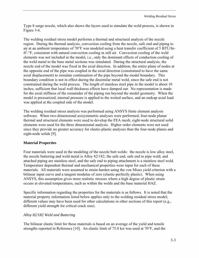
Welding Residual Stress

3-3

Type 8 surge nozzle, which also shows the layers used to simulate the weld process, is shown in Figure 3-6.

The welding residual stress model performs a thermal and structural analysis of the nozzle region. During the thermal analysis, convection cooling from the nozzle, safe end and piping to air at an ambient temperature of 70°F was modeled using a heat transfer coefficient of 5 BTU/hr-ft2-°F, consistent with natural convection cooling in still air. Convection cooling of the weld elements was not included in the model, i.e., only the dominant effects of conduction cooling of the weld metal to the base metal sections was simulated. During the structural analysis, the nozzle end of the model was fixed in the axial direction. In addition, the entire plane of nodes at the opposite end of the pipe was coupled in the axial direction (constrained to have the same axial displacement) to simulate continuation of the pipe beyond the model boundary. This boundary condition is not in effect during the dissimilar metal weld, since the safe end is not constrained during the weld process. The length of stainless steel pipe in the model is about 10 inches, sufficient that local wall thickness effects have damped out. No representation is made for the axial stiffness of the remainder of the piping run beyond the model geometry. When the model is pressurized, internal pressure is applied to the wetted surface, and an endcap axial load was applied at the coupled side of the model.

The welding residual stress analysis was performed using ANSYS finite element analysis software. When two-dimensional axisymmetric analyses were performed, four-node planar thermal and structural elements were used to develop the FEA mesh; eight-node structural solid elements were used for the three dimensional analysis. Higher order elements were not used since they provide no greater accuracy for elastic-plastic analyses than the four-node planes and eight-node solids [9].

Material Properties

Four materials were used in the modeling of the nozzle butt welds: the nozzle is low alloy steel, the nozzle buttering and weld metal is Alloy 82/182, the safe end, safe end to pipe weld, and attached piping are stainless steel, and the safe end to piping attachment is a stainless steel weld. Temperature dependent thermal and mechanical properties were input for each of these materials. All materials were assumed to strain-harden using the von Mises yield criterion with a bilinear input curve and a tangent modulus of zero (elastic-perfectly plastic). When using ANSYS, this assumption gives more realistic stresses where a high degree of plastic strain occurs at elevated temperatures, such as within the welds and the base material HAZ.

Specific information regarding the properties for the materials is as follows. It is noted that the material property information listed below applies only to the welding residual stress model; different values may have been used for other calculations in other sections of this report (e.g., different yield strength for critical crack size).

Alloy 82/182 Weld and Buttering

The bilinear elastic limit for these materials is based on an average of the yield and tensile strengths reported in Reference [10]. An elastic limit of 75.0 ksi was used at 70°F, and the

Welding Residual Stress

3-4

elastic limit at 653°F is 56.8 ksi. A Poisson’s ratio of 0.29 was used; this value was assumed to be invariant with temperature. Additional material property data were taken from a number of sources, including the 1992 ASME Boiler and Pressure Vessel Code [11], data provided by EdF for EPRI analyses [12], and Inconel product literature [10].

Low Alloy Steel Nozzle

The elastic limit values for the low alloy steel are based on typical values for the 0.2% offset yield strength of this material. An elastic limit of 50.0 ksi was used at 70°F, and the elastic limit at 653°F is 40.9 ksi. A Poisson’s ratio of 0.29 was used; this value was assumed to be invariant with temperature. Additional material property data were taken from a number of sources, including the 1992 ASME Boiler and Pressure Vessel Code [11], low alloy steel data provided by EdF for EPRI analyses [12], and research by Karlsson [13].

Stainless Steel Base Metal

The stainless steel base metal (safe end and piping) uses elastic limit values that are based on the 0.2% offset yield strength for the material. It is recognized that a small region of base metal material adjacent to the dissimilar metal and stainless steel welds will be affected by the welding process and will have a higher effective yield strength. The effect of this difference is likely bounded by the overall uncertainty of the analysis. An elastic limit of 40.0 ksi was used at 70°F, and the elastic limit at 653°F is 28.4 ksi. A Poisson’s ratio of 0.29 was used; this value was assumed to be invariant with temperature. Additional material property data were taken from a number of sources, including the 1992 ASME Boiler and Pressure Vessel Code [11], data provided by EdF for EPRI analyses [12], and research by Rybicki [14]. The values used in this analysis are identical to those used for BWR stainless steel shroud welds in [15]. Additionally, the CMTR data for the stainless steel piping materials from the plants considered in this report indicate that the values selected are appropriate (see Section 5.1).

Stainless Steel Weld Metal

The stainless steel material used to join the safe end to the piping uses material strength properties that differ from the stainless steel base metal described above. An elastic limit of 67.0 ksi was used at 70°F, and the elastic limit at 653°F is 49.8 ksi. The values for the elastic limit were taken from previous analytical work performed for BWR stainless steel shroud welds [15]. All other material property data for the weld material is the same as the base metal.

Analysis Load Steps

The welding residual stress analysis involves four general loading steps: (a) welding, (b) weld repair (if applicable), (c) hydrostatic testing, and (d) operating conditions. These processes are simulated as follows:

Welding Residual Stress

3-5

Welding Simulation

The welding process was simulated by combined thermal and structural analyses. A transient thermal analysis was used to generate nodal temperature distributions throughout the welding process. These nodal temperatures were then used as inputs to the structural analysis which calculates resultant thermally-induced stresses. The sequence of thermal analyses followed by structural analyses was duplicated for each simulated weld pass. When the model is three-dimensional, the base welding simulation was performed in an axisymmetric fashion, with welding passes simulated as rings of weld metal. In all cases, the weld passes were simulated using layers of material, with layers approximately 0.1 inches thick.

A layer-based methodology has typically been used in previous industry welding residual stress analyses for butt welds. It is recognized that the actual welds are fabricated using discrete beads, rather than layers of weld metal. However, the specific sequence and pattern of the weld beads is frequently unknown. Using a layer based approach, with the layer thickness chosen to approximate the bead size, is a way to simulate the welding process while minimizing the impact of the simulated sequence on the analysis results. Additionally, simulating certain weld repair geometries is simplified when a layer geometry is implemented. In Section 3.3, the layer-based methodology used for this work is compared to actual measured residual stresses and to the analysis results for models where a specific bead-by-bead sequence was simulated. The results shown in Section 3.3 are typical of other analysis comparisons, where a layer-based approach tends to produce similar results to bead-based models.

Heat is rapidly input to the weld pass material, using internal volumetric heat generation, at a rate which raises the peak weld metal temperature to 3,000–3,500 °F and the base metal adjacent to the weld to about 2,000 °F. These are approximately the temperatures that the weld metal and surrounding base materials reach during welding [16]. Additionally, the penetration of temperatures above 1,000°F is limited by adjusting the heat input rate and time. Rapid heating of the weld material is necessary in order to reach the desired peak weld puddle temperatures without overheating the surrounding base metal. Conversely, if the heat is applied too rapidly, the surrounding base metal materials do not reach a high enough temperature for good fusion. As noted above, thermal properties for the materials are specified in the model for temperatures up to 3,500 °F; properties at elevated temperatures are estimated or extrapolated from those at lower temperatures.

Weld Repairs

Weld repairs were simulated by deactivating elements associated with previously welded material and reapplying new weld metal in its place. Deactivation of elements essentially results in elimination of the conductive capacity and stiffness of the deactivated element in heat transfer and structural analyses, respectively. Repair welds are also done in layers approximately 0.1 inches thick.

Welding Residual Stress

3-6

Hydrostatic Testing

Components were hydrostatically tested to approximately 3,110 psig after installation. This step was included in the analysis since applied hydrostatic pressure further yields any material stressed to near yield by welding and, therefore, results in a reduction of the peak residual tensile stresses after the hydrostatic test pressure is released. In this manner, the hydrostatic testing represents a form of stress improvement in areas of high stress. In addition to applying pressure to all wetted inside surfaces, an axial tensile stress is applied to the end of the pipe equal to the longitudinal pressure stress in the pipe wall.

Operating Conditions

Operating conditions are simulated by pressurizing the inside of the model to 2,235 psig and heating all of the material uniformly to the nominal 653°F operating temperature. The pressure and thermal conditions are added to the model which has already been subjected to welding (and weld repairs) and hydrostatic testing. Operating loads due to piping forces and moments are not considered in this analysis. The operating temperature is applied first as a separate load case, since this analysis result is the one that will be used to load the fracture mechanics models.

Case Specific Analysis Steps

Because of the different geometries and conditions being considered, each of the analysis models have case-specific analysis steps. While each were done using the general procedures outlined in Section 3.2.3 above, case-specific methods were used as follows:

Type 8 Surge Nozzle

The fabrication records for the Type 8 surge nozzle show that the dissimilar metal weld has the following aspects as part of its fabrication: 1) the initial weld is built radially outwards starting from the ID, 2) the initial weld land is ground until sound weld metal is reached, 3) the ground region is rewelded to the original inner diameter, 4) the weld is inspected and any repairs are made, and 5) a fill-in weld cladding layer is deposited to seat the thermal liner. Following these weld steps, the pressurizer is delivered and the stainless steel weld is made connecting the safe end to the plant piping. This sequence is depicted in Figure 3-7, which shows the model geometry at various points during this process. This figure also shows the repaired model condition prior to starting the repair.

Type 9 Surge Nozzle

The fabrication records for this surge nozzle type indicate that it was fabricated with a smaller than nominal inner diameter, material which was then machined to the finished ID. Therefore, no inside surface finishing pass was considered for this analysis case. For this analysis case, a butt weld similar to the Type 8 weld is performed, but the inside diameter is 0.25 inches smaller than the finished radius. After completion of the weld, the inner region is analytically removed as indicated, back to the finished inside radius.

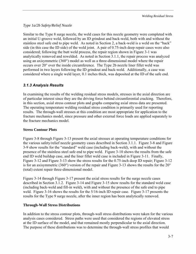
Welding Residual Stress

3-7

Type 1a/2b Safety/Relief Nozzle

Similar to the Type 8 surge nozzle, the weld cases for this nozzle geometry were completed with an initial U-groove weld, followed by an ID grindout and back-weld, both with and without the stainless steel safe end to pipe weld. As noted in Section 2, a back-weld is a weld on the “back” side (in this case the ID side) of the weld joint. A pair of 0.75-inch deep repair cases were also considered; following the butt weld process, the repair region shown in Figure 3-1 was analytically removed and rewelded. As noted in Section 3.1.1, the repair process was analyzed using an axisymmetric (360°) model as well as a three-dimensional model where the repair occurs over 20° over the inside circumference. The Type 2b nozzle liner fillet weld was performed in two layers following the ID grindout and back-weld. Additionally, a case was considered where a single weld layer, 0.1 inches thick, was deposited at the ID of the safe end.

3.1.3 Analysis Results

In examining the results of the welding residual stress models, stresses in the axial direction are of particular interest since they are the driving force behind circumferential cracking. Therefore, in this section, axial stress contour plots and graphs comparing axial stress data are presented. The operating temperature welding residual stress condition is primarily used for reporting results. The through-wall stresses at this condition are most appropriate for application to the fracture mechanics model, since pressure and other external force loads are applied separately to the fracture mechanics model.

Stress Contour Plots

Figure 3-8 through Figure 3-13 present the axial stresses at operating temperature conditions for the various safety/relief nozzle geometry cases described in Section 3.1.1. Figure 3-8 and Figure 3-9 show results for the “standard” weld case (including back-weld), with and without the presence of the stainless steel safe end to pipe weld. Figure 3-10 shows the results from the safe end ID weld buildup case, and the liner fillet weld case is included in Figure 3-11. Finally, Figure 3-12 and Figure 3-13 show the stress results for the 0.75-inch deep ID repair; Figure 3-12 is for an axisymmetric (360°) version of the repair and Figure 3-13 shows the results for the 20° (total) extent repair three-dimensional model.

Figure 3-14 through Figure 3-17 present the axial stress results for the surge nozzle cases described in Section 3.1.2. Figure 3-14 and Figure 3-15 show results for the standard weld case (including back-weld and fill-in weld), with and without the presence of the safe end to pipe weld. Figure 3-16 shows the results for the 5/16-inch ID repair case. Figure 3-17 presents the results for the Type 9 surge nozzle, after the inner region has been analytically removed.

Through-Wall Stress Distributions

In addition to the stress contour plots, through-wall stress distributions were taken for the various analysis cases considered. Stress paths were used that considered the regions of elevated stress at the ID surface of the model, and that remained mostly perpendicular to the axial direction. The purpose of these distributions was to determine the through-wall stress profiles that would

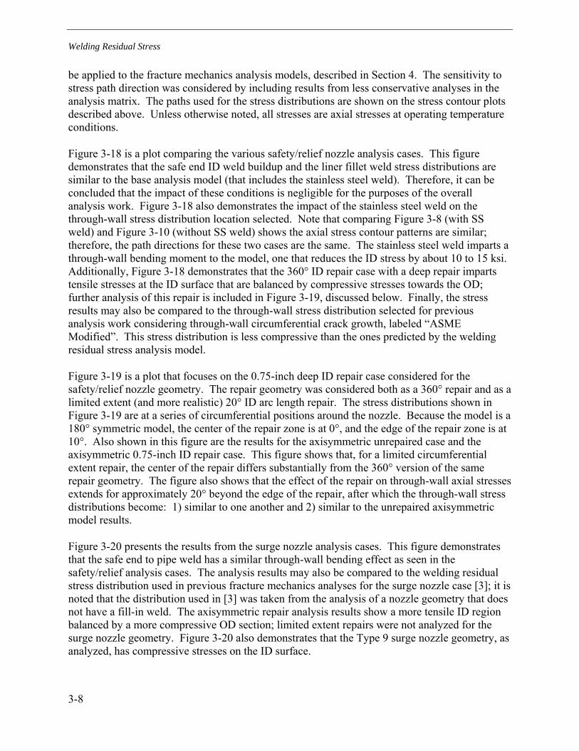
Welding Residual Stress

3-8

be applied to the fracture mechanics analysis models, described in Section 4. The sensitivity to stress path direction was considered by including results from less conservative analyses in the analysis matrix. The paths used for the stress distributions are shown on the stress contour plots described above. Unless otherwise noted, all stresses are axial stresses at operating temperature conditions.

Figure 3-18 is a plot comparing the various safety/relief nozzle analysis cases. This figure demonstrates that the safe end ID weld buildup and the liner fillet weld stress distributions are similar to the base analysis model (that includes the stainless steel weld). Therefore, it can be concluded that the impact of these conditions is negligible for the purposes of the overall analysis work. Figure 3-18 also demonstrates the impact of the stainless steel weld on the through-wall stress distribution location selected. Note that comparing Figure 3-8 (with SS weld) and Figure 3-10 (without SS weld) shows the axial stress contour patterns are similar; therefore, the path directions for these two cases are the same. The stainless steel weld imparts a through-wall bending moment to the model, one that reduces the ID stress by about 10 to 15 ksi. Additionally, Figure 3-18 demonstrates that the 360° ID repair case with a deep repair imparts tensile stresses at the ID surface that are balanced by compressive stresses towards the OD; further analysis of this repair is included in Figure 3-19, discussed below. Finally, the stress results may also be compared to the through-wall stress distribution selected for previous analysis work considering through-wall circumferential crack growth, labeled “ASME Modified”. This stress distribution is less compressive than the ones predicted by the welding residual stress analysis model.

Figure 3-19 is a plot that focuses on the 0.75-inch deep ID repair case considered for the safety/relief nozzle geometry. The repair geometry was considered both as a 360° repair and as a limited extent (and more realistic) 20° ID arc length repair. The stress distributions shown in Figure 3-19 are at a series of circumferential positions around the nozzle. Because the model is a 180° symmetric model, the center of the repair zone is at 0°, and the edge of the repair zone is at 10°. Also shown in this figure are the results for the axisymmetric unrepaired case and the axisymmetric 0.75-inch ID repair case. This figure shows that, for a limited circumferential extent repair, the center of the repair differs substantially from the 360° version of the same repair geometry. The figure also shows that the effect of the repair on through-wall axial stresses extends for approximately 20° beyond the edge of the repair, after which the through-wall stress distributions become: 1) similar to one another and 2) similar to the unrepaired axisymmetric model results.

Figure 3-20 presents the results from the surge nozzle analysis cases. This figure demonstrates that the safe end to pipe weld has a similar through-wall bending effect as seen in the safety/relief analysis cases. The analysis results may also be compared to the welding residual stress distribution used in previous fracture mechanics analyses for the surge nozzle case [3]; it is noted that the distribution used in [3] was taken from the analysis of a nozzle geometry that does not have a fill-in weld. The axisymmetric repair analysis results show a more tensile ID region balanced by a more compressive OD section; limited extent repairs were not analyzed for the surge nozzle geometry. Figure 3-20 also demonstrates that the Type 9 surge nozzle geometry, as analyzed, has compressive stresses on the ID surface.

Welding Residual Stress

3-9

3.2 WRS Literature Data

In addition to the new work on welding residual stress simulation performed in support of this project, a review of existing literature on welding residual stress was conducted. A number of papers were identified that described analysis results and residual stress measurements for axial stresses in piping butt welds, particularly in the presence of partial arc extent repairs. The papers identified the following characteristics for butt weld axial stresses:

• Repair regions tend to cause more compressive axial stresses in the approximately 20° of material beyond the edge of the repair zone [17]

• Repair regions may have significantly higher axial through-wall stresses since the repair through-wall section is balanced by the remainder of the pipe cross section [18]

As demonstrated by the results in Figure 3-13 and Figure 3-19, the welding residual stress results for the safety/relief nozzle with a partial arc repair region are in agreement with these characteristics.

3.3 Validation and Benchmarking

The finite element analysis methodologies described in this section were also used to simulate the fabrication of a mockup where residual stresses were measured and compared to analyzed residual stresses. Comparisons were performed using geometry and results from a research project completed by the European Commission Joint Research Centre’s (JRC) Institute for Energy [19]. The project investigated a wide range of issues related to the structural integrity assessment of a stainless steel weld joining stainless steel and low alloy steel components.

One of the task groups implemented by the JRC research project focused on the reliability of finite element analyses to predict residual stress in the welded joint. This task group organized a series of round-robin exercises that compared predicted welding residual stress distributions to those measured for a welded joint mockup. Complete details of the mockup geometry and welding process were made available to all participants in the round-robin, and their welding residual stress analysis results were compared to each other and to through-wall stresses measured by neutron diffraction (ND).

A drawing of the welded joint mockup as described in the round robin task group problem definition [20] is shown in Figure 3-21. This figure depicts the finished weld preparation geometry, following deposition and machining of the stainless steel butter layer on the A508 spool piece. As shown in Figure 3-21, the mockup comprised two piping spool pieces, each approximately 500 mm (20 inches) long, one made of 316L stainless steel and one from A508 low alloy steel. The weld preparation for the mockup was a V-bevel type, with the 316L piping spool forming a backing strip for the initial weld layers. The initial A508 spool piece was 64 mm (2.5 inches) thick, and the initial 316L spool piece was 73 mm (2.9 inches) thick. According to Figure 5 of [20], the dissimilar metal weld was performed in 96 total passes, comprising roughly 18 layers. Following completion of the weld, the assembly was heat treated at about 600°C (1,100°F); then the assembly was machined to the final dimensions depicted in Figure 3-21.

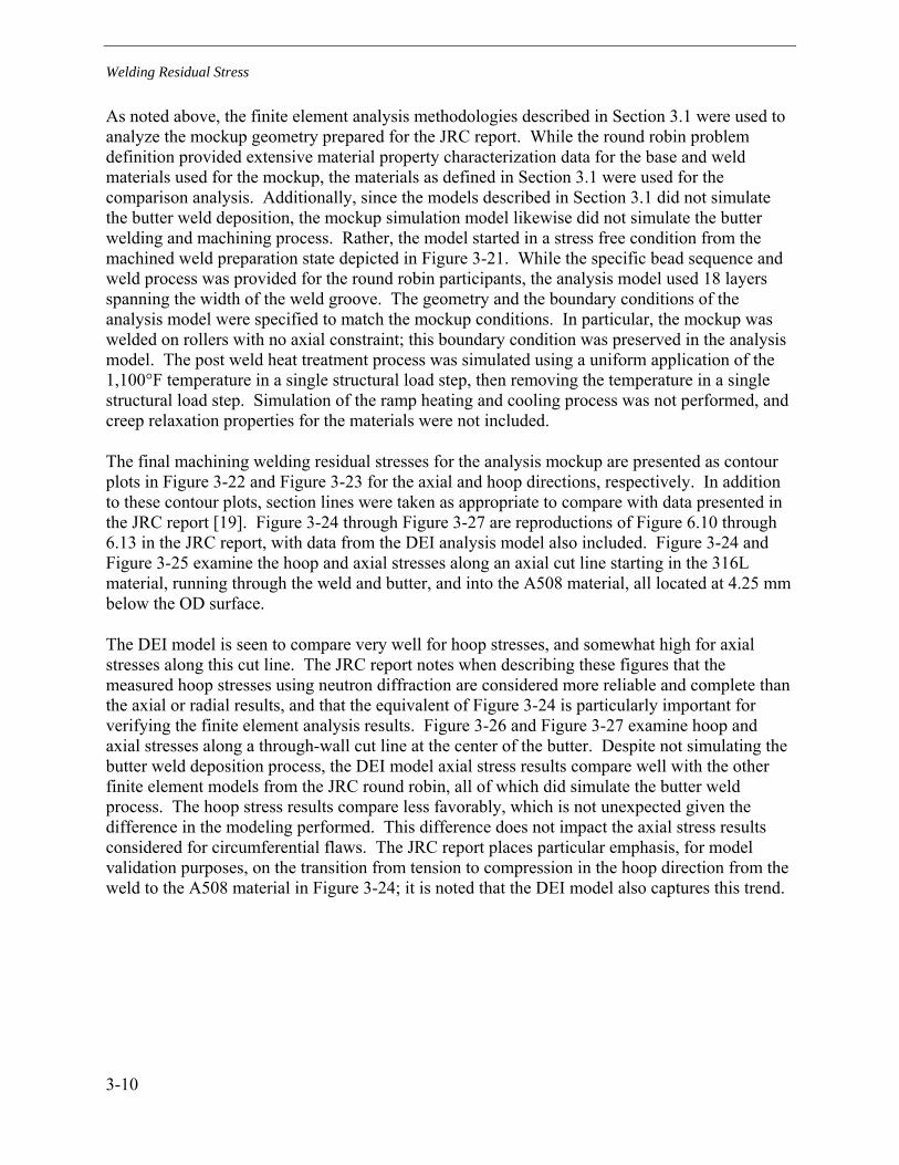
Welding Residual Stress

3-10

As noted above, the finite element analysis methodologies described in Section 3.1 were used to analyze the mockup geometry prepared for the JRC report. While the round robin problem definition provided extensive material property characterization data for the base and weld materials used for the mockup, the materials as defined in Section 3.1 were used for the comparison analysis. Additionally, since the models described in Section 3.1 did not simulate the butter weld deposition, the mockup simulation model likewise did not simulate the butter welding and machining process. Rather, the model started in a stress free condition from the machined weld preparation state depicted in Figure 3-21. While the specific bead sequence and weld process was provided for the round robin participants, the analysis model used 18 layers spanning the width of the weld groove. The geometry and the boundary conditions of the analysis model were specified to match the mockup conditions. In particular, the mockup was welded on rollers with no axial constraint; this boundary condition was preserved in the analysis model. The post weld heat treatment process was simulated using a uniform application of the 1,100°F temperature in a single structural load step, then removing the temperature in a single structural load step. Simulation of the ramp heating and cooling process was not performed, and creep relaxation properties for the materials were not included.

The final machining welding residual stresses for the analysis mockup are presented as contour plots in Figure 3-22 and Figure 3-23 for the axial and hoop directions, respectively. In addition to these contour plots, section lines were taken as appropriate to compare with data presented in the JRC report [19]. Figure 3-24 through Figure 3-27 are reproductions of Figure 6.10 through 6.13 in the JRC report, with data from the DEI analysis model also included. Figure 3-24 and Figure 3-25 examine the hoop and axial stresses along an axial cut line starting in the 316L material, running through the weld and butter, and into the A508 material, all located at 4.25 mm below the OD surface.

The DEI model is seen to compare very well for hoop stresses, and somewhat high for axial stresses along this cut line. The JRC report notes when describing these figures that the measured hoop stresses using neutron diffraction are considered more reliable and complete than the axial or radial results, and that the equivalent of Figure 3-24 is particularly important for verifying the finite element analysis results. Figure 3-26 and Figure 3-27 examine hoop and axial stresses along a through-wall cut line at the center of the butter. Despite not simulating the butter weld deposition process, the DEI model axial stress results compare well with the other finite element models from the JRC round robin, all of which did simulate the butter weld process. The hoop stress results compare less favorably, which is not unexpected given the difference in the modeling performed. This difference does not impact the axial stress results considered for circumferential flaws. The JRC report places particular emphasis, for model validation purposes, on the transition from tension to compression in the hoop direction from the weld to the A508 material in Figure 3-24; it is noted that the DEI model also captures this trend.

Welding Residual Stress

3-11

Nozzle

Clad

Safe End ID Buildup

Safe End

Pipe

Butter

Alloy 182 DMW

SS Weld

0.25"

0.38"

0.75"

Figure 3-1 Type 1a Safety/Relief Nozzle Model Geometry

Welding Residual Stress

3-12

Nozzle

LinerLiner Fillet

Weld

Safe End

Pipe

Butter

Alloy 182 DMW

SS Weld

Figure 3-2 Type 2b Safety/Relief Nozzle Model Geometry

Nozzle

CladFill-in Weld

Safe End

Pipe

Butter

Repair

Alloy 182 DMW

SS Weld

Figure 3-3 Type 8 Surge Nozzle Model Geometry

Welding Residual Stress

3-13

Nozzle

Clad

Removed Material

Safe End

Pipe

Butter

Alloy 182 DMW

SS Weld

Figure 3-4 Type 9 Surge Nozzle Model Geometry

Welding Residual Stress

3-14

Repair Zone

Figure 3-5 Safety/Relief Nozzle Repair Model Geometry

Figure 3-6 Type 8 Surge Nozzle Model – Element Mesh and Weld Layers

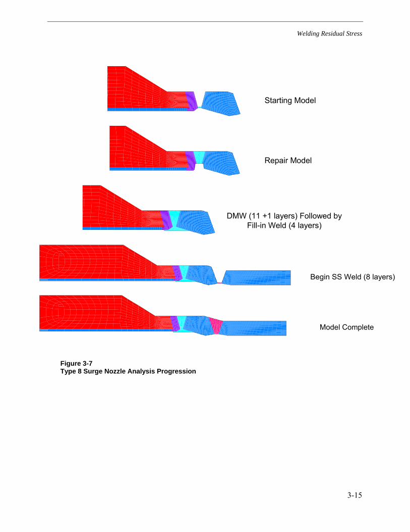
Welding Residual Stress

3-15

Starting Model

Repair Model

DMW (11 +1 layers) Followed by Fill-in Weld (4 layers)

Begin SS Weld (8 layers)

Model Complete

Figure 3-7 Type 8 Surge Nozzle Analysis Progression

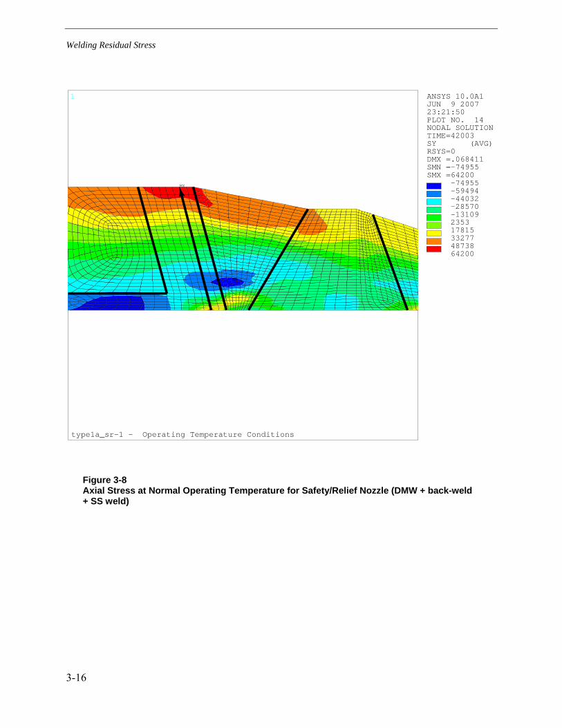
Welding Residual Stress

3-16

ANSYS 10.0A1JUN 9 200723:21:50PLOT NO. 14NODAL SOLUTIONTIME=42003SY (AVG)RSYS=0DMX =.068411SMN =-74955SMX =64200

1

MN

MX -74955-59494-44032-28570-13109235317815332774873864200

type1a_sr-1 - Operating Temperature Conditions

Figure 3-8 Axial Stress at Normal Operating Temperature for Safety/Relief Nozzle (DMW + back-weld + SS weld)

Welding Residual Stress

3-17

ANSYS 10.0A1JUN 7 200721:29:29PLOT NO. 14NODAL SOLUTIONTIME=24003SY (AVG)RSYS=0DMX =.091784SMN =-65868SMX =63013

1

MN

MX -65868-51548-37228-22907-8587573320053343734869363013

type1a_sr-3 - Operating Temperature Conditions

Figure 3-9 Axial Stress at Normal Operating Temperature for Safety/Relief Nozzle (DMW + back-weld, no SS weld)

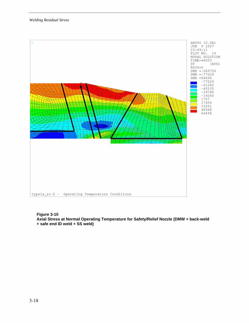
Welding Residual Stress

3-18

ANSYS 10.0A1JUN 9 200723:49:11PLOT NO. 14NODAL SOLUTIONTIME=46003SY (AVG)RSYS=0DMX =.069726SMN =-77029SMX =64696

1

MN

MX -77029-61282-45535-29788-14040170717454332014894864696

type1a_sr-2 - Operating Temperature Conditions

Figure 3-10 Axial Stress at Normal Operating Temperature for Safety/Relief Nozzle (DMW + back-weld + safe end ID weld + SS weld)

Welding Residual Stress

3-19

ANSYS 10.0A1JUN 10 200700:18:45PLOT NO. 14NODAL SOLUTIONTIME=46003SY (AVG)RSYS=0DMX =.06799SMN =-78522SMX =63619

1

MN

MX

-78522-62729-46935-31142-15348445.20316239320324782663619

type2b_sr-1 - Operating Temperature Conditions

Figure 3-11 Axial Stress at Normal Operating Temperature for Safety/Relief Nozzle (DMW + back-weld + liner fillet weld + SS weld)

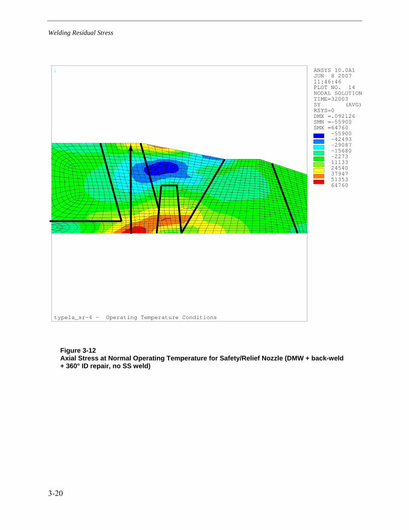
Welding Residual Stress

3-20

ANSYS 10.0A1JUN 8 200711:46:46PLOT NO. 14NODAL SOLUTIONTIME=32003SY (AVG)RSYS=0DMX =.092126SMN =-55900SMX =64760

1

MN

MX

-55900-42493-29087-15680-22731113324540379475135364760

type1a_sr-4 - Operating Temperature Conditions

Figure 3-12 Axial Stress at Normal Operating Temperature for Safety/Relief Nozzle (DMW + back-weld + 360° ID repair, no SS weld)

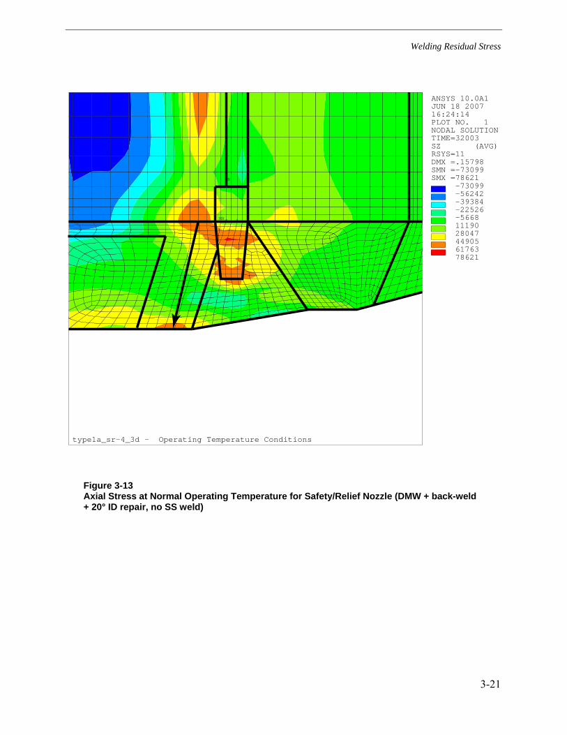
Welding Residual Stress

3-21

ANSYS 10.0A1JUN 18 200716:24:14PLOT NO. 1NODAL SOLUTIONTIME=32003SZ (AVG)RSYS=11DMX =.15798SMN =-73099SMX =78621

1

MN

MX

-73099-56242-39384-22526-56681119028047449056176378621

type1a_sr-4_3d - Operating Temperature Conditions

Figure 3-13 Axial Stress at Normal Operating Temperature for Safety/Relief Nozzle (DMW + back-weld + 20° ID repair, no SS weld)

Welding Residual Stress

3-22

ANSYS 10.0A1JUN 10 200701:00:31PLOT NO. 10NODAL SOLUTIONTIME=50003SY (AVG)RSYS=0DMX =.098933SMN =-65449SMX =62726

1

MN

MX-65449-51208-36966-22724-8483575920001342434848462726

type8_surge-1 - Operating Temperature Conditions

Figure 3-14 Axial Stress at Normal Operating Temperature for Type 8 Surge Nozzle (DMW + back-weld + fill-in weld + SS weld)

Welding Residual Stress

3-23

ANSYS 10.0A1JUN 10 200702:20:01PLOT NO. 10NODAL SOLUTIONTIME=32003SY (AVG)RSYS=0DMX =.124442SMN =-62299SMX =58553

1

MN

MX

-62299-48871-35443-22015-8587484118269316974512558553

type8_surge-3 - Operating Temperature Conditions

Figure 3-15 Axial Stress at Normal Operating Temperature for Type 8 Surge Nozzle (DMW + back-weld + fill-in weld, no SS weld)

Welding Residual Stress

3-24

ANSYS 10.0A1JUN 10 200701:46:51PLOT NO. 10NODAL SOLUTIONTIME=56003SY (AVG)RSYS=0DMX =.097629SMN =-63453SMX =63341

1

MN

MX-63453-49365-35276-21188-7100698821076351644925363341

type8_surge-2 - Operating Temperature Conditions

Figure 3-16 Axial Stress at Normal Operating Temperature for Type 8 Surge Nozzle (DMW + ID repair + fill-in weld + SS weld)

Welding Residual Stress

3-25

ANSYS 10.0A1JUN 16 200714:58:33PLOT NO. 14NODAL SOLUTIONTIME=20003SY (AVG)RSYS=0DMX =.115727SMN =-57196SMX =52051

1

MN

MX

-57196-45058-32919-20780-8642349715635277743991352051

type9_surge-1 - Operating Temperature Conditions

Figure 3-17 Axial Stress at Normal Operating Temperature for Type 9 Surge Nozzle (DMW + final machining, no SS weld)

Welding Residual Stress

3-26

-80,000

-60,000

-40,000

-20,000

0

20,000

40,000

60,000

80,000

0.000 0.100 0.200 0.300 0.400 0.500 0.600 0.700 0.800 0.900 1.000

a/t

Axi

al S

tres

s (p

si)

Type 1a-1 (base case) Type 1a-2 (safe end ID) Type 1a-3 (no SS Weld)Type 1a-4 (0.75" Repair) Type 2b-1 (liner) ASME Modified per EMC2

Legend: Type 1a-1 (base case) = DMW + back-weld + SS Weld, see Figure 3-8 Type 1a-2 (safe end ID) = DMW + back-weld + safe end ID weld + SS weld, see Figure 3-10 Type 1a-3 (no SS Weld) = DMW + back-weld, no SS Weld, see Figure 3-9 Type 1a-4 (0.75" repair) = DMW + back-weld + 360° ID repair, no SS Weld, see Figure 3-12 Type 2b-1 (liner) = DMW + back-weld + liner fillet weld + SS weld, see Figure 3-11 ASME Modified per EMC2 = Reference curve from [3]

Figure 3-18 Axial Stress Comparison – Safety/Relief Nozzle Analysis Cases

Welding Residual Stress

3-27

-80000

-60000

-40000

-20000

0

20000

40000

60000

80000

0.000 0.100 0.200 0.300 0.400 0.500 0.600 0.700 0.800 0.900 1.000

a/t

Axi

al S

tres

s (p

si)

0 10 20 30 45 60 90 180 EQUIV AXI NO REPAIR EQUIV AXI REPAIR

Legend: 0 = Center of 3D repair model, see Figure 3-13 10 = Circumferential edge of repair region, see Figure 3-13 20 – 180 = Arc length from center of repair, see Figure 3-13 EQUIV AXI NO REPAIR = Axisymmetric model with no repair, see Figure 3-9 EQUIV AXI REPAIR = Axisymmetric model with ID repair, see Figure 3-12

Figure 3-19 Axial Stress Comparison – Safety/Relief Partial Arc ID Repair Case

Welding Residual Stress

3-28

-80,000

-60,000

-40,000

-20,000

0

20,000

40,000

60,000

80,000

0.000 0.100 0.200 0.300 0.400 0.500 0.600 0.700 0.800 0.900 1.000

a/t

Axi

al S

tres

s (p

si)

Type 8-1 (base case) Type 8-2 (5/16" ID repair) Type 8-3 (no SS Weld)Type 9-1 (CE surge) Surge w/ Backweld per EMC2

Legend: Type 8-1 (base case) = DMW + back-weld + fill-in weld + SS weld, see Figure 3-14 Type 8-2 (5/16" ID repair) = DMW + ID repair + fill-in weld + SS weld, see Figure 3-16 Type 8-3 (no SS weld) = DMW + back-weld + fill-in weld, no SS weld, see Figure 3-15 Type 9-1 (CE surge) = DMW + final machining, no SS weld, see Figure 3-17 Surge w/ Back-weld per EMC2 = Reference curve from [3]

Figure 3-20 Axial Stress Comparison – Surge Nozzle Analysis Cases

Welding Residual Stress

3-29

Figure 3-21 Welding Residual Stress Validation Mockup Drawing [20]

7.2

mm

11.5

0 m

m

25°

316L

A508

SS B

utte

r

Rem

oved

Mat

eria

l

Rem

oved

Mat

eria

l

510

mm

530

mm

ø 467 mm

ø 453 mm

ø 351 mm

ø 321 mm

ø 339 mm

Welding Residual Stress

3-30

ANSYS 10.0A1JUL 18 200723:24:39PLOT NO. 1NODAL SOLUTIONSTEP=1479SUB =6TIME=36003SY (AVG)RSYS=0DMX =.268985SMN =-46996SMX =63193

1

MN

MX

-46996-34753-22509-1026619771422026463387065094963193

eurr_ad01 - Welding Resid + Machining Final

Figure 3-22 Validation Model Axial Stress Results – Final Machining

Welding Residual Stress

3-31

ANSYS 10.0A1JUL 18 200723:24:48PLOT NO. 2NODAL SOLUTIONSTEP=1479SUB =6TIME=36003SZ (AVG)RSYS=0DMX =.268985SMN =-63378SMX =76072

1

MN

MX

-63378-47883-32389-16895-14001409429589450836057776072

eurr_ad01 - Welding Resid + Machining Final

Figure 3-23 Validation Model Hoop Stress Results – Final Machining

Welding Residual Stress

3-32

-400

-200

0

200

400

600

800

-60 -40 -20 0 20 40 60

Dist from Weld C/L (mm)

Hoo

p St

ress

(4.2

5 m

m b

elow

out

er s

urfa

ce) (

MPa

) .

ND Measurements AREVA NP SAS inspecta AREVA NP GmbH JRC DEI/EPRI

316L 508

316L 309 weld butter A508

Figure 3-24 Validation Model Predicted vs. Measured Results, Hoop Direction, 4.25 mm Below the Outer Surface

Welding Residual Stress

3-33

-200

-100

0

100

200

300

400

-60 -40 -20 0 20 40 60

Dist from Weld C/L (mm)

Axi

al S

tres

s (4

.25

mm

bel

ow o

uter

sur

face

) (M

Pa)

.

ND Measurements AREVA NP SAS inspecta AREVA NP GmbH JRC DEI/EPRI

316L 508

316L 309 weld butter A508

Figure 3-25 Validation Model Predicted vs. Measured Results, Axial Direction, 4.25 mm Below the Outer Surface

Welding Residual Stress

3-34

-500

-400

-300

-200

-100

0

100

200

300

400

500

0 10 20 30 40 50

Radial Dist from Outer Surface (mm)

Hoo

p St

ress

(MPa

)

ND Measurements AREVA NP SAS inspecta AREVA NP GmbH JRC DEI/EPRI

316L 508

Figure 3-26 Validation Model Predicted vs. Measured Results, Hoop Direction, Through-Wall Section at Butter Layer Center

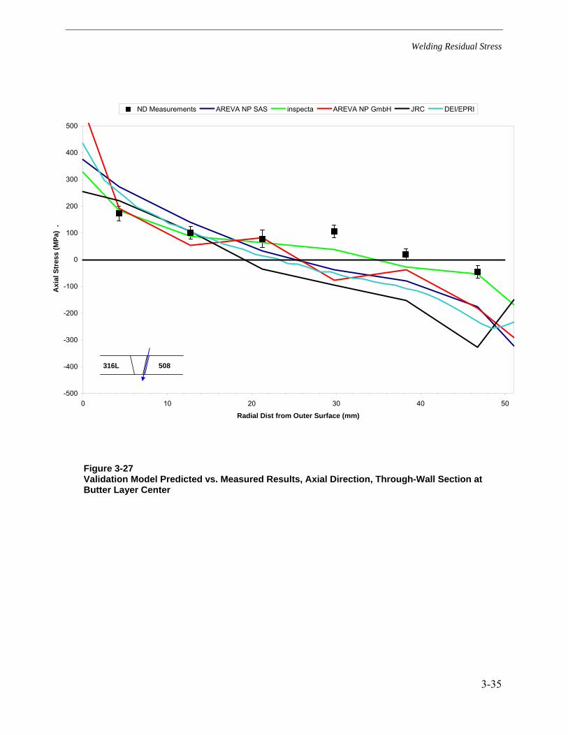
Welding Residual Stress

3-35

-500

-400

-300

-200

-100

0

100

200

300

400

500

0 10 20 30 40 50

Radial Dist from Outer Surface (mm)

Axi

al S

tres

s (M

Pa)

.

ND Measurements AREVA NP SAS inspecta AREVA NP GmbH JRC DEI/EPRI

316L 508

Figure 3-27 Validation Model Predicted vs. Measured Results, Axial Direction, Through-Wall Section at Butter Layer Center

4-1

4 CRACK GROWTH MODELING

The purpose of this section is to describe the fracture mechanics and crack growth calculations that were used to take into account the change in flaw shape that will occur with varying crack tip stress intensity factors (SIFs, also denoted as K) along the crack front. These calculations were performed using software developed specifically to consider crack growth with an arbitrary profile geometry. This section describes the overall approach used for the calculations. Additional results from a sensitivity matrix of loading cases are provided in Section 7. This section also includes, as an example, the detailed results from the Phase I portion of the overall work scope, where the loads and initial flaw geometry used in previous flaw growth analyses were used to perform the arbitrary profile crack growth calculations.

4.1 Modeling Approach

4.1.1 FEA Model

Cylindrical FEA Model

Finite element analysis was used to calculate the crack tip stress intensity factor (SIF) for all flaws considered in this calculation. Figure 4-1 shows the FEA model geometry for a typical starting surface flaw case. As shown in Figure 4-1, the analysis model is three-dimensional and is symmetric about both the plane of the flaw and about the deepest point of the flaw (quarter symmetric). The geometries of the nozzle welds are simplified to be represented by a basic cylindrical geometry with a strip of material representing the weld. As shown in Section 2 and Section 3 of this report, the actual geometry of the dissimilar metal welds is a single U-groove attachment to a safe end, which then transitions in thickness and diameter over a short length to the attached piping. The simplified geometry assumption permits more analysis cases to be performed since the models are smaller and solve more quickly. Additionally, the simplified cylindrical geometry more readily permits application of arbitrary through-wall stress distributions. The effect of the actual nozzle geometry is also considered as part of the sensitivity case matrix in Section 7.

The meshes generated for this calculation make use of 8-node brick elements, with collapsed-front crack-tip nodes. The 8-node brick elements were used for their computational efficiency, particularly for cases where contact surfaces were being used. The crack front region of the fracture mechanics model’s mesh is detailed in Figure 4-1. This figure shows the arrangement of the nodes near the crack front region, demonstrating the concentric rings of nodes that radiate outwards from the crack front location. The rings are used to perform J-integral calculations as part of the analysis model post-processing.

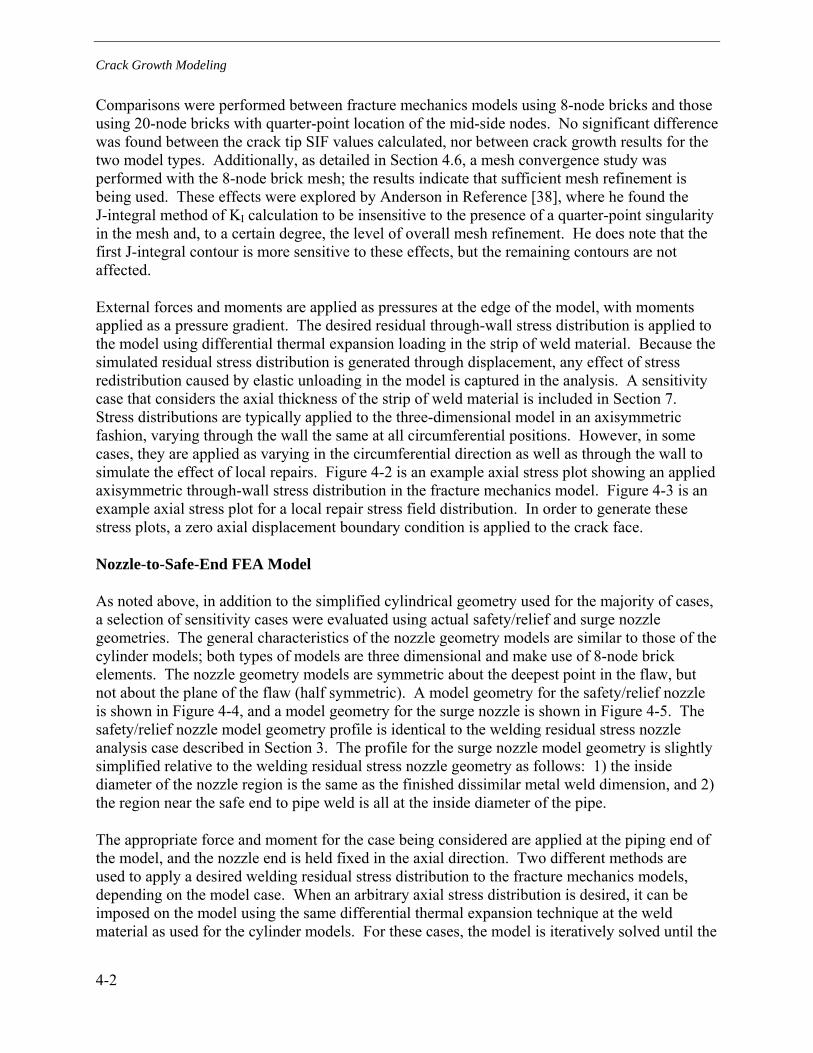
Crack Growth Modeling

4-2

Comparisons were performed between fracture mechanics models using 8-node bricks and those using 20-node bricks with quarter-point location of the mid-side nodes. No significant difference was found between the crack tip SIF values calculated, nor between crack growth results for the two model types. Additionally, as detailed in Section 4.6, a mesh convergence study was performed with the 8-node brick mesh; the results indicate that sufficient mesh refinement is being used. These effects were explored by Anderson in Reference [38], where he found the J-integral method of KI calculation to be insensitive to the presence of a quarter-point singularity in the mesh and, to a certain degree, the level of overall mesh refinement. He does note that the first J-integral contour is more sensitive to these effects, but the remaining contours are not affected.

External forces and moments are applied as pressures at the edge of the model, with moments applied as a pressure gradient. The desired residual through-wall stress distribution is applied to the model using differential thermal expansion loading in the strip of weld material. Because the simulated residual stress distribution is generated through displacement, any effect of stress redistribution caused by elastic unloading in the model is captured in the analysis. A sensitivity case that considers the axial thickness of the strip of weld material is included in Section 7. Stress distributions are typically applied to the three-dimensional model in an axisymmetric fashion, varying through the wall the same at all circumferential positions. However, in some cases, they are applied as varying in the circumferential direction as well as through the wall to simulate the effect of local repairs. Figure 4-2 is an example axial stress plot showing an applied axisymmetric through-wall stress distribution in the fracture mechanics model. Figure 4-3 is an example axial stress plot for a local repair stress field distribution. In order to generate these stress plots, a zero axial displacement boundary condition is applied to the crack face.

Nozzle-to-Safe-End FEA Model

As noted above, in addition to the simplified cylindrical geometry used for the majority of cases, a selection of sensitivity cases were evaluated using actual safety/relief and surge nozzle geometries. The general characteristics of the nozzle geometry models are similar to those of the cylinder models; both types of models are three dimensional and make use of 8-node brick elements. The nozzle geometry models are symmetric about the deepest point in the flaw, but not about the plane of the flaw (half symmetric). A model geometry for the safety/relief nozzle is shown in Figure 4-4, and a model geometry for the surge nozzle is shown in Figure 4-5. The safety/relief nozzle model geometry profile is identical to the welding residual stress nozzle analysis case described in Section 3. The profile for the surge nozzle model geometry is slightly simplified relative to the welding residual stress nozzle geometry as follows: 1) the inside diameter of the nozzle region is the same as the finished dissimilar metal weld dimension, and 2) the region near the safe end to pipe weld is all at the inside diameter of the pipe.

The appropriate force and moment for the case being considered are applied at the piping end of the model, and the nozzle end is held fixed in the axial direction. Two different methods are used to apply a desired welding residual stress distribution to the fracture mechanics models, depending on the model case. When an arbitrary axial stress distribution is desired, it can be imposed on the model using the same differential thermal expansion technique at the weld material as used for the cylinder models. For these cases, the model is iteratively solved until the

Crack Growth Modeling

4-3

through-wall temperature distribution results in the desired stress distribution at the location of the crack plane. Example cases of imposed through-wall distributions are shown in Figure 4-6 and Figure 4-7. In order to generate these stress plots, the crack faces are held coupled together.

In addition to the arbitrary stress distributions considered for the safety/relief and surge nozzle cases, a safety/relief case was also considered where the welding residual stresses were interpolated into the fracture mechanics model geometry. The interpolation process includes the complete triaxial stress state of the model, rather than axial stresses alone. The stress state for the fracture mechanics model is an elastic one based on the elastic-plastic stress state of the welding residual stress model. Therefore, all calculations are based in linear elastic fracture mechanics. The starting welding residual stress model for this case includes the complete nozzle butt weld, but without the stainless steel weld. The circumferential flaw in the fracture mechanics model was placed at the axial location of highest ID axial stress (see Figure 3-9). The axial stresses resulting from the imposed stress distribution for the fracture mechanics model are shown in Figure 4-8. Comparing the welding residual stress model results to those resulting from interpolation, it is demonstrated that the interpolation process generates a model stress distribution that closely resembles the welding model stress state. Similar to other analysis models, the crack face is loaded with pressure and the piping end of the model is loaded with axial force and bending moment prior to being solved.

4.1.2 Calculation of Crack Tip Stress Intensity Factor

Because the model is linear elastic, the J-integral calculations are not of the total strain energy (since there is no plastic strain), but of the elastic strain energy, frequently referred to as G. For convenience and for consistency with the software outputs, the strain energy values calculated from the ANSYS results files (using an external program called FEACrack, see Section 4.2) are hereafter referred to as J values. Using the relationship between J and K for the special case of linear elastic materials and using plane strain conditions, the crack tip stress intensity is calculated from the J-integral values with the following equation:

'K J E= × [4-1]

where,

K = crack tip stress intensity factor (psi√in) J = calculated J-integral value (psi•in) E' = E / (1-ν2) E = Young’s modulus ν = Poisson’s ratio = 0.30

It is noted that the J-integral value calculated by the software results from Mode I loading due to the symmetry boundary conditions of the model.

Crack Growth Modeling

4-4

4.1.3 Crack Growth for an Arbitrary Flaw Shape

Once the crack tip SIF along the entire front has been calculated, the results are used to determine the shape of the flaw after a small time increment has passed. The crack growth increment at each point (i.e., node) on the crack front is based on the SIF calculated at that point, with growth occurring in the direction normal to the crack front. The crack growth rate is calculated using the SIF in combination with the MRP-115 [21] crack growth rate equation for Alloy 182 weld metal, which recommends a SIF exponent of 1.6 and the use of a zero SIF threshold. Sensitivity cases for the SIF-dependence of the crack growth rate are also performed as part of the case matrix described in Section 7.

The crack growth rate values were input directly to the FEACrack software. The change in crack profile for each growth step and the time required for each growth step are calculated in a fully explicit manner from the previous step, based on an input step size for growth at the point of maximum SIF.

It should be recognized that the standard assumption of uniform and isotropic material resistance to PWSCC crack growth is assumed in the crack growth simulations. However, weld metal materials, including Alloy 82/182 piping butt welds, have a complex and anisotropic microstructure that can result in significant spatial and directional variability in the crack growth rate [21]. Furthermore, laboratory experience often shows a fingerlike crack front pattern, indicating greater through-wall extension in comparison to lateral extension than would be expected for the case of uniform and isotropic material resistance. This sort of behavior is commonly observed in the laboratory compact tension specimens used to measure PWSCC crack growth rate in Alloy 82/182 weld materials [21]. In 2004, EPRI published an MRP-sponsored laboratory study [41] that investigated the effect of weld metal microstructure on PWSCC initiation and growth in pressurized test capsules fabricated from Alloy 182 weld metal material. With regard to patterns of crack extension observed, this study concluded the following:

“The cracks exhibited an unusual aspect ratio in that they never showed a large lateral surface extent, even when they extended through the wall thickness. This is a very different feature compared to PWSCC in Ni-base alloys such as Alloy 600. The aspect ratio is thought to relate to indications of crack arrest observed at low energy grain boundaries in Alloy 182.”

The laboratory studies of capsule and compact tension specimens indicate that actual crack growth behavior in Alloy 82/182 weld metal materials is likely to be more favorable toward through-wall penetration and leakage occurring prior to rupture than is predicted under the standard assumption of uniform and isotropic material resistance. This is because actual effective growth rates in the lateral (i.e., circumferential) direction for a circumferential surface flaw on the weld ID may be lower in comparison to the growth rate in the depth direction (toward through-wall penetration and leakage) than is predicted by models assuming uniform and isotropic dependence of the crack growth rate on the SIF in combination with high assumed axial stresses around the ID surface.

Crack Growth Modeling

4-5

4.1.4 Flaw Shape Transition

For every fracture mechanics analysis case considered in the sensitivity case matrix described in Section 7, the initial flaw is either a partially circumferential or fully circumferential (depending on the case) ID surface flaw. The flaw is allowed to grow at an appropriately refined growth step until the deepest part reaches about 93% of the wall thickness. At this point, the flaw size is projected to where the deepest part reaches 100% wall thickness, and a new, through-wall (either true through-wall or complex crack) mesh is generated. In some cases, a partially circumferential ID surface flaw reaches around to become a fully circumferential ID surface flaw before it reaches through-wall; an intermediate variable depth circumferential surface flaw profile is generated in these cases. When the new through-wall mesh geometry is generated, the projected crack front from the surface flaw case is used as the through-wall flaw profile, and any regions where the remaining ligament is less than 10% of the wall thickness are converted to an open crack face (forming the through wall or complex crack). In this way, thin ligaments of material are assumed to break through immediately, without taking credit for additional time to grow through the region. An example of this mesh transition is included in Figure 4-9, which shows the final step of the surface crack growth and the first step of the complex crack growth.

4.2 Fracture Mechanics Calculation Software Background

The fracture mechanics model geometry is generated by FEACrack, a specialized fracture mechanics pre- and post-processing software code. The base model geometry, the model external loads, and the initial flaw geometry were all defined with the FEACrack software. Using this information, the software generates a finite element mesh that may be solved to calculate the stress state of the model. FEACrack is not a finite element analysis code; however, it is capable of automating the process used to generate a mesh and analyze that mesh on a variety of commercial analysis software codes. The analyses of the fracture mechanics models were performed using ANSYS Version 10.0, installed on the same computer as FEACrack.

Once the model is analyzed, the post-processing portion of FEACrack reads the ANSYS results and performs J-integral calculations at a number of points along the crack front. J-integral calculations are performed at each of five concentric rings set around the collapsed crack front nodes to determine an average J-integral value. The contour integral closest to the crack front is not used in the calculation; this does not impact the accuracy of the calculation. The variation of the average from each of the individual J-integral values determines the “contour dependence” of the average J-integral value, and is performed as an internal check on the numerical accuracy and mesh refinement of the FEA model. The J-integral contour dependencies are generally verified to be lower than 5% per the recommendation of the fracture mechanics software. The exception is at the one or two points near the surface of the flaw. Anderson notes in [38] that the J-integral value at the surface point of the flaw is frequently difficult to calculate with path independence. When this occurs, FEACrack will linearly extrapolate the J-integral value for the points where the path dependence is high, basing the extrapolation on previous values along the crack front.

FEACrack also has the capability of interleaving pre- and post-processing of a fracture mechanics model with the model analysis solution in ANSYS to perform crack growth analysis calculations. The crack growth analysis sequence is as follows: an initial mesh is generated, the

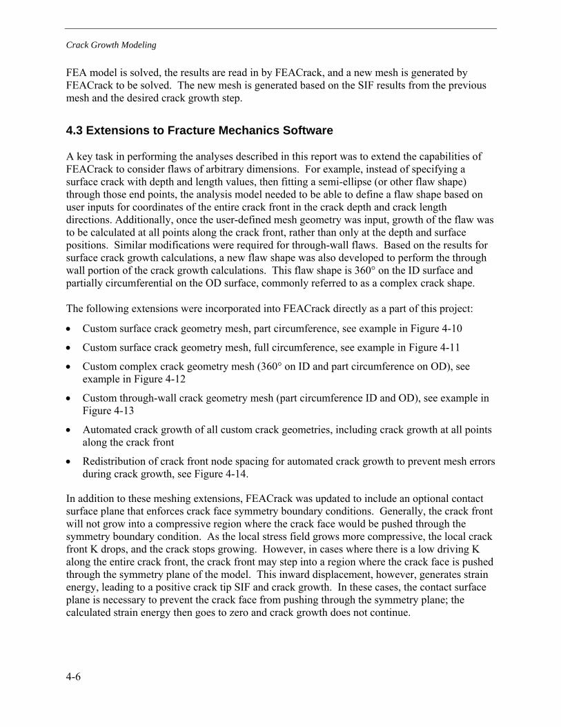
Crack Growth Modeling

4-6

FEA model is solved, the results are read in by FEACrack, and a new mesh is generated by FEACrack to be solved. The new mesh is generated based on the SIF results from the previous mesh and the desired crack growth step.

4.3 Extensions to Fracture Mechanics Software

A key task in performing the analyses described in this report was to extend the capabilities of FEACrack to consider flaws of arbitrary dimensions. For example, instead of specifying a surface crack with depth and length values, then fitting a semi-ellipse (or other flaw shape) through those end points, the analysis model needed to be able to define a flaw shape based on user inputs for coordinates of the entire crack front in the crack depth and crack length directions. Additionally, once the user-defined mesh geometry was input, growth of the flaw was to be calculated at all points along the crack front, rather than only at the depth and surface positions. Similar modifications were required for through-wall flaws. Based on the results for surface crack growth calculations, a new flaw shape was also developed to perform the through wall portion of the crack growth calculations. This flaw shape is 360° on the ID surface and partially circumferential on the OD surface, commonly referred to as a complex crack shape.

The following extensions were incorporated into FEACrack directly as a part of this project:

• Custom surface crack geometry mesh, part circumference, see example in Figure 4-10

• Custom surface crack geometry mesh, full circumference, see example in Figure 4-11

• Custom complex crack geometry mesh (360° on ID and part circumference on OD), see example in Figure 4-12

• Custom through-wall crack geometry mesh (part circumference ID and OD), see example in Figure 4-13

• Automated crack growth of all custom crack geometries, including crack growth at all points along the crack front

• Redistribution of crack front node spacing for automated crack growth to prevent mesh errors during crack growth, see Figure 4-14.

In addition to these meshing extensions, FEACrack was updated to include an optional contact surface plane that enforces crack face symmetry boundary conditions. Generally, the crack front will not grow into a compressive region where the crack face would be pushed through the symmetry boundary condition. As the local stress field grows more compressive, the local crack front K drops, and the crack stops growing. However, in cases where there is a low driving K along the entire crack front, the crack front may step into a region where the crack face is pushed through the symmetry plane of the model. This inward displacement, however, generates strain energy, leading to a positive crack tip SIF and crack growth. In these cases, the contact surface plane is necessary to prevent the crack face from pushing through the symmetry plane; the calculated strain energy then goes to zero and crack growth does not continue.

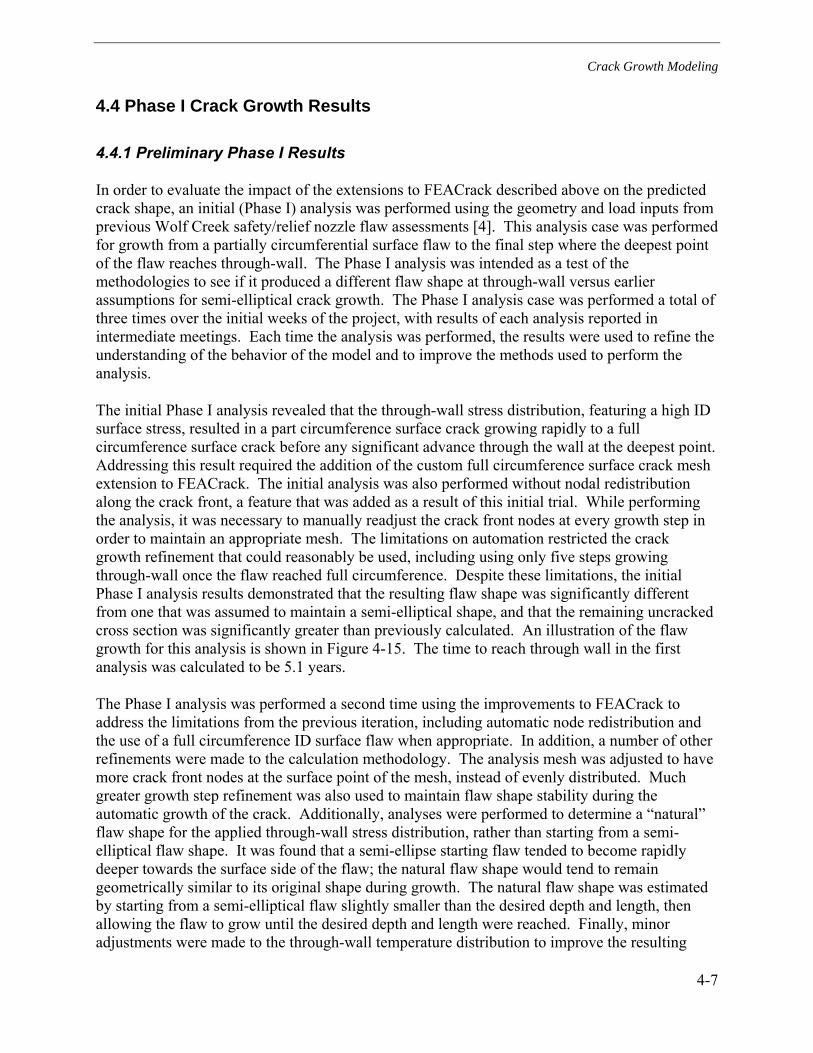
Crack Growth Modeling

4-7

4.4 Phase I Crack Growth Results

4.4.1 Preliminary Phase I Results

In order to evaluate the impact of the extensions to FEACrack described above on the predicted crack shape, an initial (Phase I) analysis was performed using the geometry and load inputs from previous Wolf Creek safety/relief nozzle flaw assessments [4]. This analysis case was performed for growth from a partially circumferential surface flaw to the final step where the deepest point of the flaw reaches through-wall. The Phase I analysis was intended as a test of the methodologies to see if it produced a different flaw shape at through-wall versus earlier assumptions for semi-elliptical crack growth. The Phase I analysis case was performed a total of three times over the initial weeks of the project, with results of each analysis reported in intermediate meetings. Each time the analysis was performed, the results were used to refine the understanding of the behavior of the model and to improve the methods used to perform the analysis.

The initial Phase I analysis revealed that the through-wall stress distribution, featuring a high ID surface stress, resulted in a part circumference surface crack growing rapidly to a full circumference surface crack before any significant advance through the wall at the deepest point. Addressing this result required the addition of the custom full circumference surface crack mesh extension to FEACrack. The initial analysis was also performed without nodal redistribution along the crack front, a feature that was added as a result of this initial trial. While performing the analysis, it was necessary to manually readjust the crack front nodes at every growth step in order to maintain an appropriate mesh. The limitations on automation restricted the crack growth refinement that could reasonably be used, including using only five steps growing through-wall once the flaw reached full circumference. Despite these limitations, the initial Phase I analysis results demonstrated that the resulting flaw shape was significantly different from one that was assumed to maintain a semi-elliptical shape, and that the remaining uncracked cross section was significantly greater than previously calculated. An illustration of the flaw growth for this analysis is shown in Figure 4-15. The time to reach through wall in the first analysis was calculated to be 5.1 years.

The Phase I analysis was performed a second time using the improvements to FEACrack to address the limitations from the previous iteration, including automatic node redistribution and the use of a full circumference ID surface flaw when appropriate. In addition, a number of other refinements were made to the calculation methodology. The analysis mesh was adjusted to have more crack front nodes at the surface point of the mesh, instead of evenly distributed. Much greater growth step refinement was also used to maintain flaw shape stability during the automatic growth of the crack. Additionally, analyses were performed to determine a “natural” flaw shape for the applied through-wall stress distribution, rather than starting from a semi-elliptical flaw shape. It was found that a semi-ellipse starting flaw tended to become rapidly deeper towards the surface side of the flaw; the natural flaw shape would tend to remain geometrically similar to its original shape during growth. The natural flaw shape was estimated by starting from a semi-elliptical flaw slightly smaller than the desired depth and length, then allowing the flaw to grow until the desired depth and length were reached. Finally, minor adjustments were made to the through-wall temperature distribution to improve the resulting

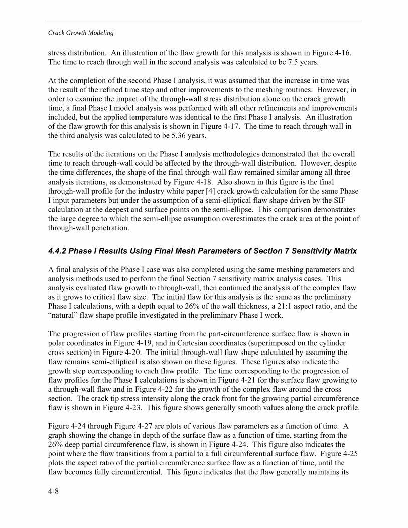
Crack Growth Modeling

4-8

stress distribution. An illustration of the flaw growth for this analysis is shown in Figure 4-16. The time to reach through wall in the second analysis was calculated to be 7.5 years.

At the completion of the second Phase I analysis, it was assumed that the increase in time was the result of the refined time step and other improvements to the meshing routines. However, in order to examine the impact of the through-wall stress distribution alone on the crack growth time, a final Phase I model analysis was performed with all other refinements and improvements included, but the applied temperature was identical to the first Phase I analysis. An illustration of the flaw growth for this analysis is shown in Figure 4-17. The time to reach through wall in the third analysis was calculated to be 5.36 years.

The results of the iterations on the Phase I analysis methodologies demonstrated that the overall time to reach through-wall could be affected by the through-wall distribution. However, despite the time differences, the shape of the final through-wall flaw remained similar among all three analysis iterations, as demonstrated by Figure 4-18. Also shown in this figure is the final through-wall profile for the industry white paper [4] crack growth calculation for the same Phase I input parameters but under the assumption of a semi-elliptical flaw shape driven by the SIF calculation at the deepest and surface points on the semi-ellipse. This comparison demonstrates the large degree to which the semi-ellipse assumption overestimates the crack area at the point of through-wall penetration.

4.4.2 Phase I Results Using Final Mesh Parameters of Section 7 Sensitivity Matrix

A final analysis of the Phase I case was also completed using the same meshing parameters and analysis methods used to perform the final Section 7 sensitivity matrix analysis cases. This analysis evaluated flaw growth to through-wall, then continued the analysis of the complex flaw as it grows to critical flaw size. The initial flaw for this analysis is the same as the preliminary Phase I calculations, with a depth equal to 26% of the wall thickness, a 21:1 aspect ratio, and the “natural” flaw shape profile investigated in the preliminary Phase I work.

The progression of flaw profiles starting from the part-circumference surface flaw is shown in polar coordinates in Figure 4-19, and in Cartesian coordinates (superimposed on the cylinder cross section) in Figure 4-20. The initial through-wall flaw shape calculated by assuming the flaw remains semi-elliptical is also shown on these figures. These figures also indicate the growth step corresponding to each flaw profile. The time corresponding to the progression of flaw profiles for the Phase I calculations is shown in Figure 4-21 for the surface flaw growing to a through-wall flaw and in Figure 4-22 for the growth of the complex flaw around the cross section. The crack tip stress intensity along the crack front for the growing partial circumference flaw is shown in Figure 4-23. This figure shows generally smooth values along the crack profile.

Figure 4-24 through Figure 4-27 are plots of various flaw parameters as a function of time. A graph showing the change in depth of the surface flaw as a function of time, starting from the 26% deep partial circumference flaw, is shown in Figure 4-24. This figure also indicates the point where the flaw transitions from a partial to a full circumferential surface flaw. Figure 4-25 plots the aspect ratio of the partial circumference surface flaw as a function of time, until the flaw becomes fully circumferential. This figure indicates that the flaw generally maintains its

Crack Growth Modeling

4-9

long aspect ratio as it grows around the circumference. Figure 4-26 plots the percentage of the cylinder surface area covered by the flaw as a function of time, showing the surface crack (both partial and full circumference) and complex crack regimes of crack growth. The small discontinuities in the area at the transitions result from the assumed ligament breaking as the flaw reaches the edge of the section. Figure 4-27 shows the flaw shape function as a function of time; the shape function is defined as the actual flaw cross section divided by the cross sectional area of a semi-elliptical flaw with the same depth and length. This figure indicates that the flaw initially has a larger area than the equivalent semi-ellipse, but quickly develops a shape that has a smaller cross section than the equivalent semi-ellipse.

Figure 4-28 is a plot showing the stability margin on load as a function of time, starting from the initial partial circumference surface flaw and progressing to a complex flaw until a load factor of 1.0 is reached. As shown in this figure, the partial circumference flaw starts with a large margin on load that progresses steadily downward as the flaw grows through-wall. The load factor and leak rate as a function of time once the flaw reaches through-wall are shown in Figure 4-29; this plot is similar to plots in Section 7 for other sensitivity matrix cases. The figures shows that for the Phase I case, a time of about 70 days is required for the flaw to grow from 1 gpm leakage to a stability margin on load of 1.2.

4.5 Stress Intensity Factor Verification

The methodologies used in this report to generate, solve, and post-process a finite element analysis mesh for an arbitrary surface crack front profile were compared to an independent calculation performed by EMC2, a contractor to the NRC, as a means of benchmarking the calculations. A set of four proposed crack front profiles were generated from specified combinations of mathematical functions. By defining them in terms of analytical functions, the profiles are completely defined for any arbitrary grid spacing and are not dependent on a particular mesh refinement. The four profiles selected are shown in Figure 4-30, both in planar coordinates and in the cylindrical coordinates used to generate the actual mesh. A common set of external loads (membrane plus bending stress) were applied to the crack models.

The calculation was performed using FEACrack to generate the mesh, ANSYS to solve the FEA mesh, and FEACrack to post-process the analysis results and calculate the crack tip SIF along the crack front. The independent calculation performed by EMC2 used their own software to generate the mesh, and ABAQUS to solve the model and calculate the crack tip SIF along the crack front. The comparison for K solutions for all four crack fronts is shown in Figure 4-31. This figure demonstrates excellent agreement between the two independent analyses.

4.6 Crack Growth Convergence Checks

4.6.1 Temporal Convergence Check

As noted above, the amount of growth between successive crack growth steps is a specified parameter in the crack growth analysis, and the cumulative amount of time required to grow the specified distance is an output from the analysis. If the specified growth step is too large to

Crack Growth Modeling

4-10

capture the variations in loading through the wall of the model, an inaccurate final crack size will result. In order to check that sufficient growth refinement was being used, comparisons were performed for surface crack and complex crack growth progressions with about twice the normal growth step refinement. This convergence check is referred to as the temporal convergence check since a reduced growth step size also corresponds to refinement in the time step size.

Case 1c defined in Section 7, which corresponds to an initial 10% through-wall 360° surface flaw, was used as the base case for this study. The normal surface crack growth procedure was applied in each case, with a growth step of 0.040 inches for the base case versus a growth step of 0.016 inches for the refined case. Additionally, the final growth step was made from a depth of 93% through-wall to 100% through-wall because of the difficulty in meshing very deep flaws. For the complex crack portion of the convergence check, the cracks were grown from the same initial complex crack profile, with both the original and refined growth step size until a desired number of steps were achieved. For the refined growth step size case, the step size was halved and the number of growth steps doubled, resulting in the same final crack length on the weld OD. The complex flaw base case growth step is 0.072 inches, versus a refined case growth step of 0.036 inches.

The comparison results for the temporal convergence check are shown in Table 4-1 and Figure 4-32, which demonstrate an acceptably small level of temporal numerical convergence error. The final surface crack and complex crack profiles are nearly identical for the case of varying growth step size. Based on these results, it is concluded that a sufficient level of growth step refinement is assumed in the sensitivity matrix of crack growth calculations of Section 7.

4.6.2 Spatial Convergence Check

In addition to the preceding temporal convergence check, a spatial grid refinement convergence study was also performed using the same initial surface crack and complex crack cases. For the refined grid case, the number of elements in the radial and axial directions was increased by about 50%. The number of elements in the circumferential direction was maintained at the same normal level because of a software limitation.

The comparison results for the spatial convergence check are shown in Table 4-1 and Figure 4-33, which also demonstrate an acceptably small level of spatial numerical convergence error. The final surface crack and complex crack profiles are nearly identical for the case of varying grid refinement. Based on these results and the relatively large number of nodes assumed in the circumferential direction (typically 100 over 180°), it is concluded that a sufficient level of grid refinement is assumed in the sensitivity matrix of crack growth calculations of Section 7.

4.7 Validation Cases

As a consistency check of the ability of the crack growth methodology described above to predict actual plant experience, the large circumferential crack detected at the BWR Duane Arnold plant was applied as a validation case. A cross section through the 360° part-depth crack at Duane Arnold is shown in Figure 4-34 [22]. Crack initiation and growth were attributed to the

Crack Growth Modeling

4-11

presence of a fully circumferential crevice that led to development of an acidic environment because of the oxygen in the normal BWR water chemistry, combined with high residual and applied stresses as a result of the geometry and nearby welds, including the unusual repair weld made on the outside of the Alloy 600 safe end to correct a safe end fabrication error. The water chemistry conditions that contributed to cracking at Duane Arnold do not exist for the case of Alloy 82/182 piping butt welds in PWR plants.

In order to apply the Duane Arnold experience to the crack growth methodology described above, a welding residual stress analysis of the Duane Arnold configuration, including the weld repair, was performed [23]. The calculated through-wall variation in welding residual stress (including application of normal operating temperature but not pressure) at the general crack location is shown in Figure 4-35. The polynomial fit shown in this figure was assumed in the validation case, as were reported operating pressure and design piping loads [23].

The crack profile calculated in the validation check is shown in Figure 4-36 versus the actual Duane Arnold crack profile. This profile is based on the assumption of an initial 30% through-wall uniform depth 360° surface flaw, in combination with the MRP-115 [21] crack growth rate dependence on stress intensity factor. (The assumption of an initial 360° surface flaw is reasonable given that the crevice between the thermal sleeve and safe end is expected to have acted as a crack starter.) The agreement shown in the predicted and actual crack profiles in Figure 4-36 is reasonable. However, because the simulated crack profile attained is sensitive to the particular assumed initial crack profile and no information is available on the actual crack profile at earlier times, this validation case must be interpreted as a consistency check of the crack growth methodology versus the Duane Arnold experience. In addition, it is recognized that the effective turn in flaw direction from the axial direction of the crevice to the general radial direction of the crack is a complication that cannot be directly addressed by the crack growth methodology.

Crack Growth Modeling

4-12

Table 4-1 Results of Temporal and Spatial Convergence Study for Case 1 360° Surface and Complex Crack Growth Progressions

CaseSensitivity Description

Time(years)(Note 1)

%Difference

in Time

MaximumAbsolute

Differencein Depth (in)

Maximum Abs.Difference in IDCircumferential

Position (in)

30 Steps - Original Mesh Base Case 17.42

70 Steps - Original Mesh Temporal 17.18 -1.40% 0.0158 0.0102

30 Steps - Refined Mesh Spatial 17.21 -1.24% 0.0021 0.0005

65 Steps - Original Mesh Base Case 0.725

130 Steps - Original Mesh Temporal 0.701 -3.27% 0.0127 0.0371

65 Steps - Refined Mesh Spatial 0.721 -0.52% 0.0013 0.0021

Note 1: Time for the 360° surface crack case is time to through-wall and for the complex crack case is time until desired number of steps has been executed.

360°

Sur

face

Cra

ckC

ompl

exC

rack

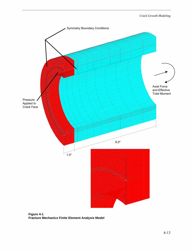
Crack Growth Modeling

4-13

1.0"

8.0"

Symmetry Boundary Conditions

PressureApplied toCrack Face

Axial Forceand EffectiveTotal Moment

1

Figure 4-1 Fracture Mechanics Finite Element Analysis Model

Crack Growth Modeling

4-14

ANSYS 10.0A1JUL 9 200701:10:00PLOT NO. 1NODAL SOLUTIONSTEP=1SUB =1TIME=1SX (AVG)RSYS=0DMX =.225E-03SMN =-22240SMNB=-22546SMX =61901SMXB=65277

1

MN

MX

-22240-12891-35425807151562450533854432035255261901

Figure 4-2 Axisymmetric Through Wall Stress Distribution Example

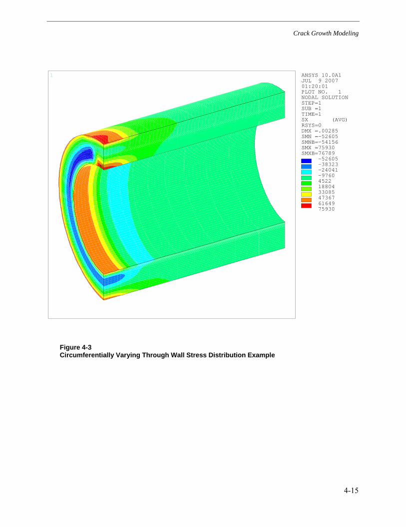
Crack Growth Modeling

4-15

ANSYS 10.0A1JUL 9 200701:20:01PLOT NO. 1NODAL SOLUTIONSTEP=1SUB =1TIME=1SX (AVG)RSYS=0DMX =.00285SMN =-52605SMNB=-54156SMX =75930SMXB=76789

1

MN

MX

-52605-38323-24041-976045221880433085473676164975930

Figure 4-3 Circumferentially Varying Through Wall Stress Distribution Example

Crack Growth Modeling

4-16

Symmetry Plane

Axial Forceand EffectiveTotal Moment

Figure 4-4 Safety/Relief Nozzle Fracture Mechanics Model (Nozzle Geometry)

Crack Growth Modeling

4-17

Symmetry Plane

Axial Forceand EffectiveTotal Moment

Figure 4-5 Surge Nozzle Fracture Mechanics Model (Nozzle Geometry)

Crack Growth Modeling

4-18

ANSYS 10.0A1JUL 27 200715:31:23PLOT NO. 1NODAL SOLUTIONSTEP=1SUB =1TIME=1SX (AVG)RSYS=0DMX =.614E-03SMN =-21656SMNB=-23104SMX =66424SMXB=68894

1

MN

MX

-21656-11869-20827704174912727837064468515663866424

Figure 4-6 Safety Nozzle Imposed Axial Through Wall Stress Distribution

Crack Growth Modeling

4-19

ANSYS 10.0A1JUL 27 200715:48:10PLOT NO. 1NODAL SOLUTIONSTEP=1SUB =1TIME=1SX (AVG)RSYS=0DMX =.840E-03SMN =-32101SMNB=-34028SMX =54798SMXB=56802

1

MN

MX

-32101-22445-12790-313565211617625832354874514254798

Figure 4-7 Surge Nozzle Imposed Axial Through Wall Stress Distribution

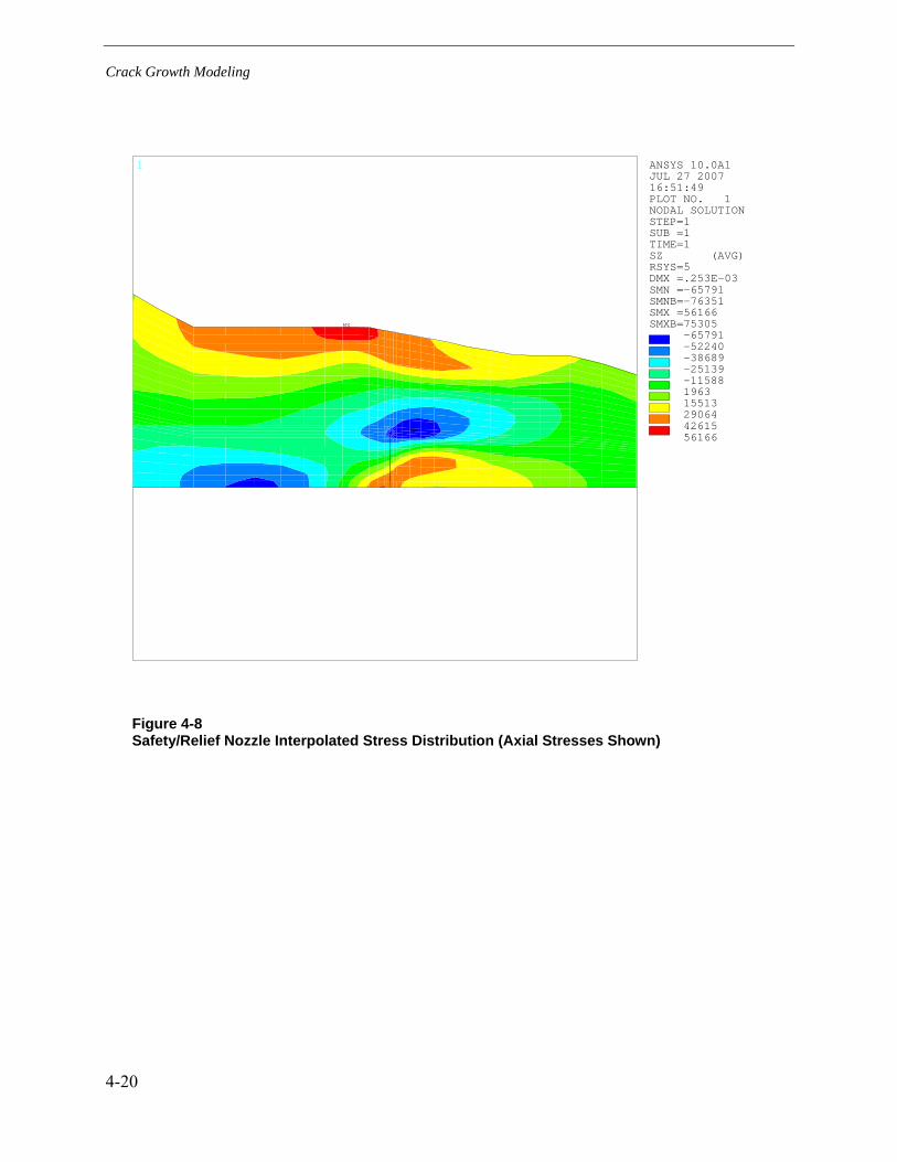
Crack Growth Modeling

4-20

ANSYS 10.0A1JUL 27 200716:51:49PLOT NO. 1NODAL SOLUTIONSTEP=1SUB =1TIME=1SZ (AVG)RSYS=5DMX =.253E-03SMN =-65791SMNB=-76351SMX =56166SMXB=75305

1

MN

MX

-65791-52240-38689-25139-11588196315513290644261556166

Figure 4-8 Safety/Relief Nozzle Interpolated Stress Distribution (Axial Stresses Shown)

Crack Growth Modeling

4-21

Figure 4-9 Example Mesh Transition from Surface Flaw to Complex Flaw

Crack Growth Modeling

4-22

Figure 4-10 Part Circumference Custom Surface Crack Geometry Example

Crack Growth Modeling

4-23

Figure 4-11 Full Circumference Custom Surface Crack Geometry Example

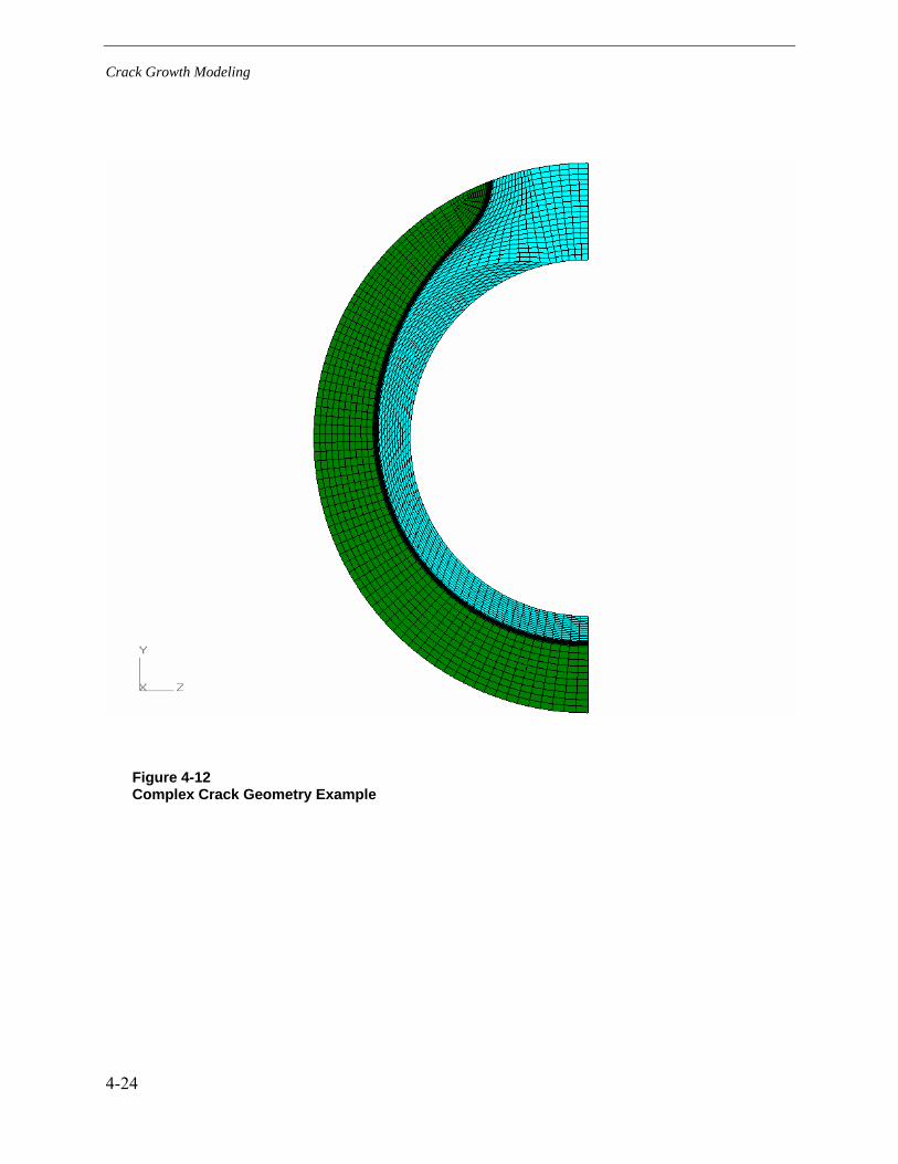
Crack Growth Modeling

4-24

Figure 4-12 Complex Crack Geometry Example

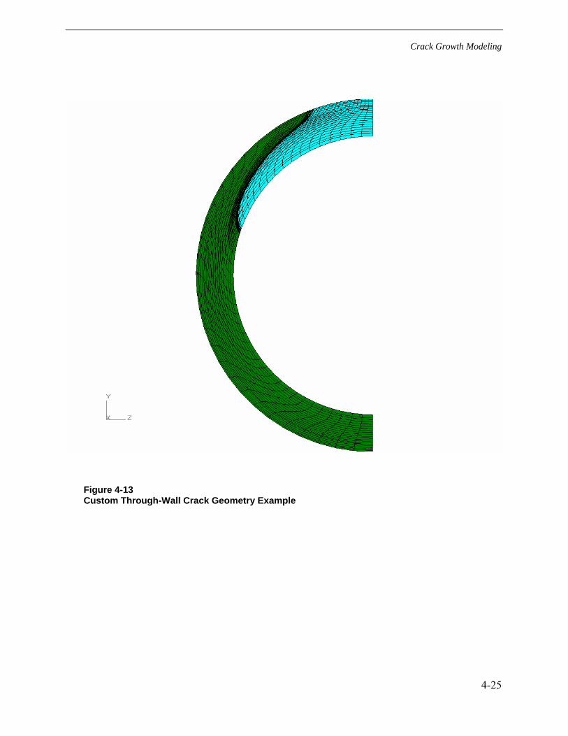
Crack Growth Modeling

4-25

Figure 4-13 Custom Through-Wall Crack Geometry Example

Crack Growth Modeling

4-26

Figure 4-14 Illustration of Crack Front Redistribution During Crack Growth Calculations

Crack Growth Modeling

4-27

0.00

0.20

0.40

0.60

0.80

1.00

1.20

0.0 1.0 2.0 3.0 4.0 5.0 6.0 7.0 8.0

Circumferential Distance Along ID (in)

Cra

ck D

epth

(in)

a/t = 0.260; 2c/a = 20.999 a/t = 0.324; 2c/a = 17.702 a/t = 0.346; 2c/a = 17.375 a/t = 0.362; 2c/a = 17.344a/t = 0.378; 2c/a = 17.365 a/t = 0.391; 2c/a = 17.487 a/t = 0.403; 2c/a = 17.639 a/t = 0.414; 2c/a = 17.829a/t = 0.425; 2c/a = 18.028 a/t = 0.435; 2c/a = 18.243 a/t = 0.445; 2c/a = 18.464 a/t = 0.454; 2c/a = 18.692a/t = 0.463; 2c/a = 18.917 a/t = 0.472; 2c/a = 19.130 a/t = 0.482; 2c/a = 19.325 a/t = 0.492; 2c/a = 19.505a/t = 0.502; 2c/a = 19.665 a/t = 0.512; 2c/a = 19.804 a/t = 0.523; 2c/a = 19.916 a/t = 0.535; 2c/a = 19.996a/t = 0.547; 2c/a = 20.041 a/t = 0.560; 2c/a = 20.063 a/t = 0.575; 2c/a = 20.027 a/t = 0.591; 2c/a = 19.939a/t = 0.610; 2c/a = 19.784 a/t = 0.631; 2c/a = 19.551 a/t = 0.686; 2c/a = 18.003 a/t = 0.740; 2c/a = 16.682a/t = 0.794; 2c/a = 15.542 a/t = 0.848; 2c/a = 14.548 a/t = 0.900; 2c/a = 13.712 a/t = 1.000; 2c/a = 12.341

t = wall thickness = 1.29 in

This approximate region also expected to be cracked at time of through-wall penetration(estimated wall area fraction of 0.014);360° surface crack model needed to assess precisely

Figure 4-15 Phase I Initial Calculation Flaw Profile Growth (with Initial Semi-Elliptical Flaw Shape)

Crack Growth Modeling

4-28

0.00

0.20

0.40

0.60

0.80

1.00

1.20

0.0 1.0 2.0 3.0 4.0 5.0 6.0 7.0 8.0

Circumferential Distance Along ID (in)

Cra

ck D

epth

(in)

2c/a=20.9, a/t=0.260 2c/a=18.9, a/t=0.310 2c/a=18.4, a/t=0.342 2c/a=18.5, a/t=0.375 2c/a=19.0, a/t=0.395

2c/a=19.5, a/t=0.413 2c/a=20.0, a/t=0.428 2c/a=20.5, a/t=0.439 2c/a=21.3, a/t=0.454 2c/a=21.9, a/t=0.466

2c/a=22.6, a/t=0.481 2c/a=23.1, a/t=0.493 2c/a=ID circ, a/t=0.493 2c/a=ID circ, a/t=0.548 2c/a=ID circ, a/t=0.626

2c/a=ID circ, a/t=0.703 2c/a=ID circ, a/t=0.781 2c/a=ID circ, a/t=0.858 2c/a=ID circ, a/t=0.936 2c/a=ID circ, a/t=1.000

Figure 4-16 Phase I Second Calculation Flaw Profile Growth (with Initial “Natural” Flaw Shape)

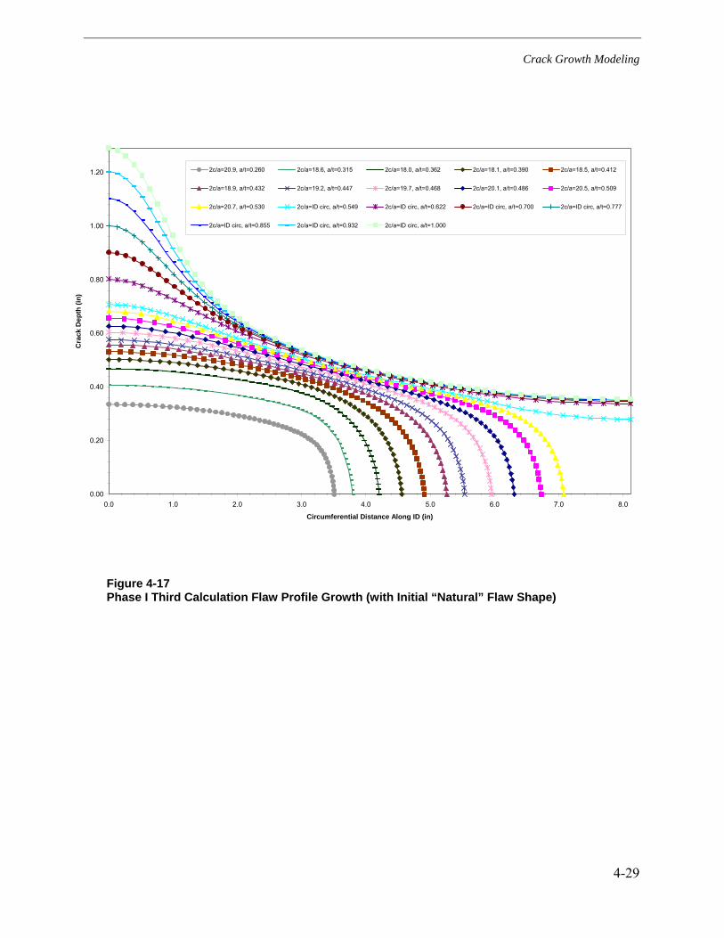
Crack Growth Modeling

4-29

0.00

0.20

0.40

0.60

0.80

1.00

1.20

0.0 1.0 2.0 3.0 4.0 5.0 6.0 7.0 8.0

Circumferential Distance Along ID (in)

Cra

ck D

epth

(in)

2c/a=20.9, a/t=0.260 2c/a=18.6, a/t=0.315 2c/a=18.0, a/t=0.362 2c/a=18.1, a/t=0.390 2c/a=18.5, a/t=0.412

2c/a=18.9, a/t=0.432 2c/a=19.2, a/t=0.447 2c/a=19.7, a/t=0.468 2c/a=20.1, a/t=0.486 2c/a=20.5, a/t=0.509

2c/a=20.7, a/t=0.530 2c/a=ID circ, a/t=0.549 2c/a=ID circ, a/t=0.622 2c/a=ID circ, a/t=0.700 2c/a=ID circ, a/t=0.777

2c/a=ID circ, a/t=0.855 2c/a=ID circ, a/t=0.932 2c/a=ID circ, a/t=1.000

Figure 4-17 Phase I Third Calculation Flaw Profile Growth (with Initial “Natural” Flaw Shape)

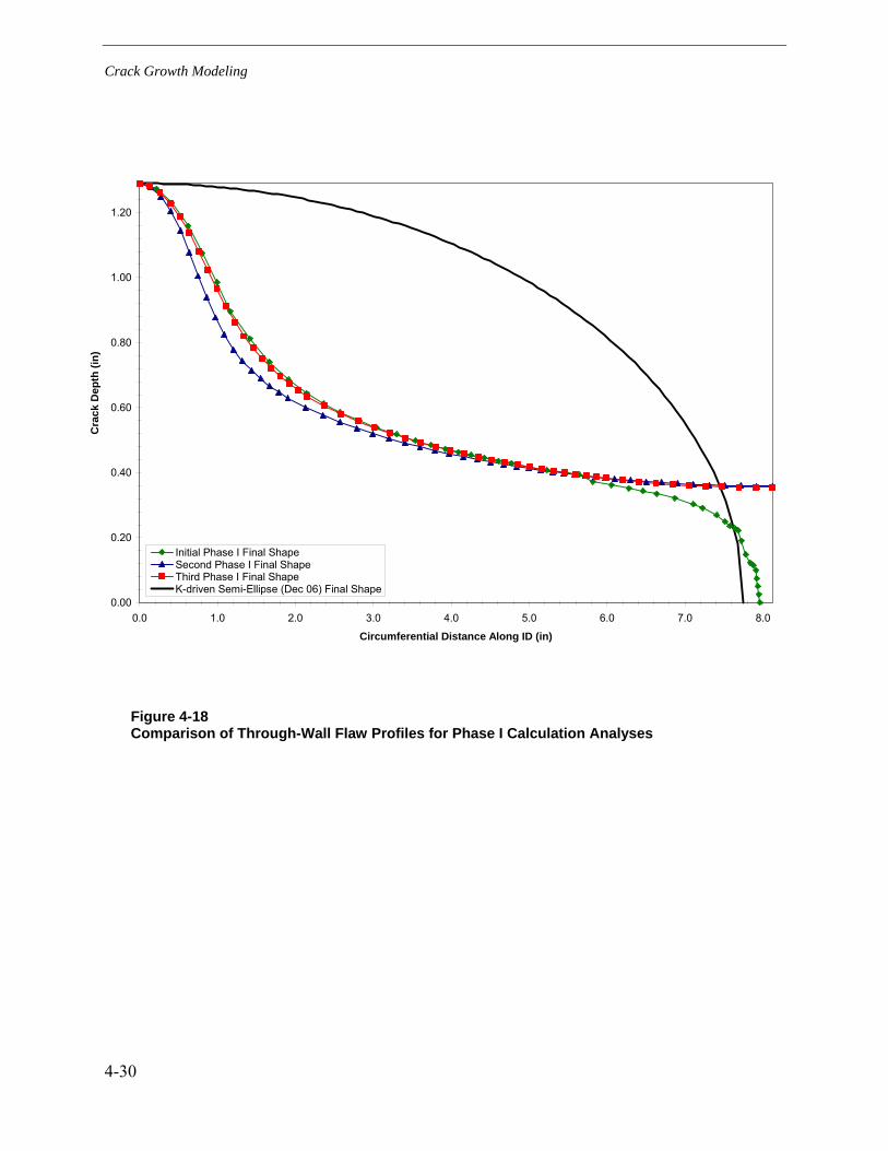
Crack Growth Modeling

4-30

0.00

0.20

0.40

0.60

0.80

1.00

1.20

0.0 1.0 2.0 3.0 4.0 5.0 6.0 7.0 8.0

Circumferential Distance Along ID (in)

Cra

ck D

epth

(in)

Initial Phase I Final ShapeSecond Phase I Final ShapeThird Phase I Final ShapeK-driven Semi-Ellipse (Dec 06) Final Shape

Figure 4-18 Comparison of Through-Wall Flaw Profiles for Phase I Calculation Analyses

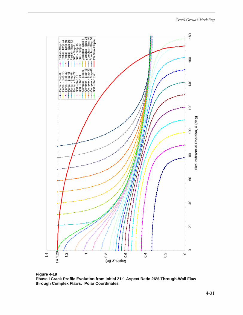
Crack Growth Modeling

4-31

Figure 4-19 Phase I Crack Profile Evolution from Initial 21:1 Aspect Ratio 26% Through-Wall Flaw through Complex Flaws: Polar Coordinates

0

0.2

0.4

0.6

0.81

1.2

1.4

020

4060

8010

012

014

016

018

0

Circ

umfe

rent

ial P

ositi

on, θ

(deg

)

Depth, y (in)

Par

tial -

Ste

p 0

Par

tial -

Ste

p 8

Par

tial -

Ste

p 16

Par

tial -

Ste

p 24

Par

tial -

Ste

p 32

Par

tial -

Ste

p 40

Par

tial -

Ste

p 48

Par

tial -

Ste

p 56

Par

tial -

Ste

p 64

Par

tial -

Ste

p 72

Par

tial -

Ste

p 77

360

- Ste

p 6

360

- Ste

p 12

360

- Ste

p 18

360

- Ste

p 24

360

- Ste

p 32

Com

plex

- S

tep

0C

ompl

ex -

Ste

p 8

Com

plex

- S

tep

16C

ompl

ex -

Ste

p 24

Com

plex

- S

tep

32C

ompl

ex -

Ste

p 40

Com

plex

- S

tep

48C

ompl

ex -

Ste

p 56

360

- Ste

p TW

TW S

emi-E

llips

e

t = 1

.29

Crack Growth Modeling

4-32

-4.00

-3.00

-2.00

-1.00

0.00

1.00

2.00

3.00

4.00

-4.5 -3.5 -2.5 -1.5 -0.5

Z (in)

Y (in

)

Complex - Step 0 Complex - Step 8Complex - Step 16 Complex - Step 24Complex - Step 32 Complex - Step 40Complex - Step 48 Complex - Step 56Partial - Step 0 Partial - Step 8Partial - Step 16 Partial - Step 24Partial - Step 32 Partial - Step 40Partial - Step 48 Partial - Step 56Partial - Step 64 Partial - Step 72Partial - Step 77 360 - Step 0360 - Step 6 360 - Step 12360 - Step 18 360 - Step 24360 - Step 32 360 - Step TWSemi-Ellipse

Figure 4-20 Phase I Crack Profile Evolution from Initial 21:1 Aspect Ratio 26% Through-Wall Flaw through Complex Flaws: Cartesian Coordinates

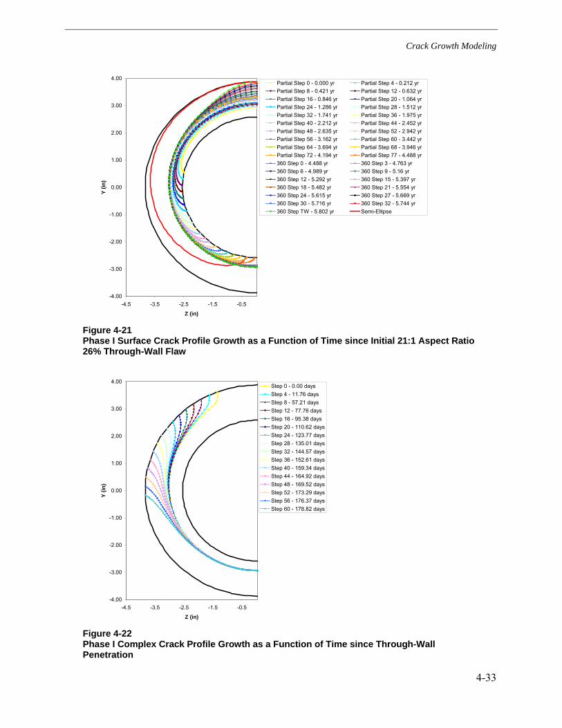
Crack Growth Modeling

4-33

-4.00

-3.00

-2.00

-1.00

0.00

1.00

2.00

3.00

4.00

-4.5 -3.5 -2.5 -1.5 -0.5

Z (in)

Y (in

)

Partial Step 0 - 0.000 yr Partial Step 4 - 0.212 yrPartial Step 8 - 0.421 yr Partial Step 12 - 0.632 yrPartial Step 16 - 0.846 yr Partial Step 20 - 1.064 yrPartial Step 24 - 1.286 yr Partial Step 28 - 1.512 yrPartial Step 32 - 1.741 yr Partial Step 36 - 1.975 yrPartial Step 40 - 2.212 yr Partial Step 44 - 2.452 yrPartial Step 48 - 2.635 yr Partial Step 52 - 2.942 yrPartial Step 56 - 3.162 yr Partial Step 60 - 3.442 yrPartial Step 64 - 3.694 yr Partial Step 68 - 3.946 yrPartial Step 72 - 4.194 yr Partial Step 77 - 4.488 yr360 Step 0 - 4.488 yr 360 Step 3 - 4.763 yr360 Step 6 - 4.989 yr 360 Step 9 - 5.16 yr360 Step 12 - 5.292 yr 360 Step 15 - 5.397 yr360 Step 18 - 5.482 yr 360 Step 21 - 5.554 yr360 Step 24 - 5.615 yr 360 Step 27 - 5.669 yr360 Step 30 - 5.716 yr 360 Step 32 - 5.744 yr360 Step TW - 5.802 yr Semi-Ellipse

Figure 4-21 Phase I Surface Crack Profile Growth as a Function of Time since Initial 21:1 Aspect Ratio 26% Through-Wall Flaw

-4.00

-3.00

-2.00

-1.00

0.00

1.00

2.00

3.00

4.00

-4.5 -3.5 -2.5 -1.5 -0.5

Z (in)

Y (in

)

Step 0 - 0.00 daysStep 4 - 11.76 daysStep 8 - 57.21 daysStep 12 - 77.76 daysStep 16 - 95.38 daysStep 20 - 110.62 daysStep 24 - 123.77 daysStep 28 - 135.01 daysStep 32 - 144.57 daysStep 36 - 152.61 daysStep 40 - 159.34 daysStep 44 - 164.92 daysStep 48 - 169.52 daysStep 52 - 173.29 daysStep 56 - 176.37 daysStep 60 - 178.82 days

Figure 4-22 Phase I Complex Crack Profile Growth as a Function of Time since Through-Wall Penetration

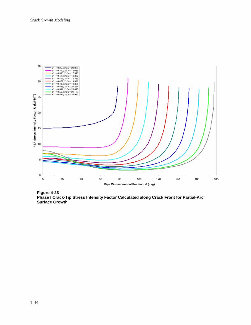
Crack Growth Modeling

4-34

0

5

10

15

20

25

30

35

0 20 40 60 80 100 120 140 160 180

Pipe Circumferential Position, θ (deg)

FEA

Str

ess

Inte

nsity

Fac

tor,

K (k

si-in

0.5 )

a/t = 0.259; 2c/a = 20.929a/t = 0.342; 2c/a = 18.069a/t = 0.386; 2c/a = 17.943a/t = 0.418; 2c/a = 18.332a/t = 0.445; 2c/a = 18.863a/t = 0.471; 2c/a = 19.391a/t = 0.498; 2c/a = 19.825a/t = 0.523; 2c/a = 20.299a/t = 0.544; 2c/a = 20.840a/t = 0.568; 2c/a = 21.197a/t = 0.594; 2c/a = 20.913

Figure 4-23 Phase I Crack-Tip Stress Intensity Factor Calculated along Crack Front for Partial-Arc Surface Growth

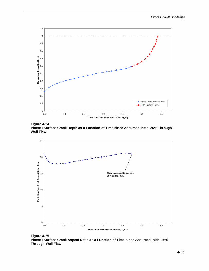
Crack Growth Modeling

4-35

0

0.1

0.2

0.3

0.4

0.5

0.6

0.7

0.8

0.9

1

1.1

0.0 1.0 2.0 3.0 4.0 5.0 6.0

Time since Assumed Initial Flaw, T (yrs)

Nor

mal

ized

Cra

ck D

epth

, y/t

Partial-Arc Surface Crack360° Surface Crack

Figure 4-24 Phase I Surface Crack Depth as a Function of Time since Assumed Initial 26% Through-Wall Flaw

0

5

10

15

20

25

0.0 1.0 2.0 3.0 4.0 5.0 6.0

Time since Assumed Initial Flaw, t (yrs)

Part

ial S

urfa

ce C

rack

Asp

ect R

atio

, 2c/

a

Flaw calculated to become 360° surface flaw

Figure 4-25 Phase I Surface Crack Aspect Ratio as a Function of Time since Assumed Initial 26% Through-Wall Flaw

Crack Growth Modeling

4-36

0

0.1

0.2

0.3

0.4

0.5

0.6

0.0 1.0 2.0 3.0 4.0 5.0 6.0

Time Since Assumed Initial Flaw, t (yrs)

Cra

ck A

rea

Frac

tion

(Cra

ck A

rea

/ Wel

d C

ross

Sec

tion

Are

a)Partial-Arc Surface Crack

360° Surface Crack

Complex Through-Wall Crack

Partial-Arc to360° Surface Crack

360° Surface to Complex TW Crack

Figure 4-26 Phase I Surface and Complex Crack Area Fraction as a Function of Time since Assumed Initial 26% Through-Wall Flaw

0.0

0.2

0.4

0.6

0.8

1.0

1.2

0.0 1.0 2.0 3.0 4.0 5.0 6.0

Time Since Assumed Initial Flaw, t (yrs)

Flaw

Sha

pe F

acto

r(C

rack

Are

a / A

rea

of S

emi-E

llips

e w

ith S

ame

Leng

th a

nd D

epth

)

Flaw calculated to become 360° surface flaw

Figure 4-27 Phase I Surface Crack Shape Factor as a Function of Time since Assumed Initial 26% Through-Wall Flaw

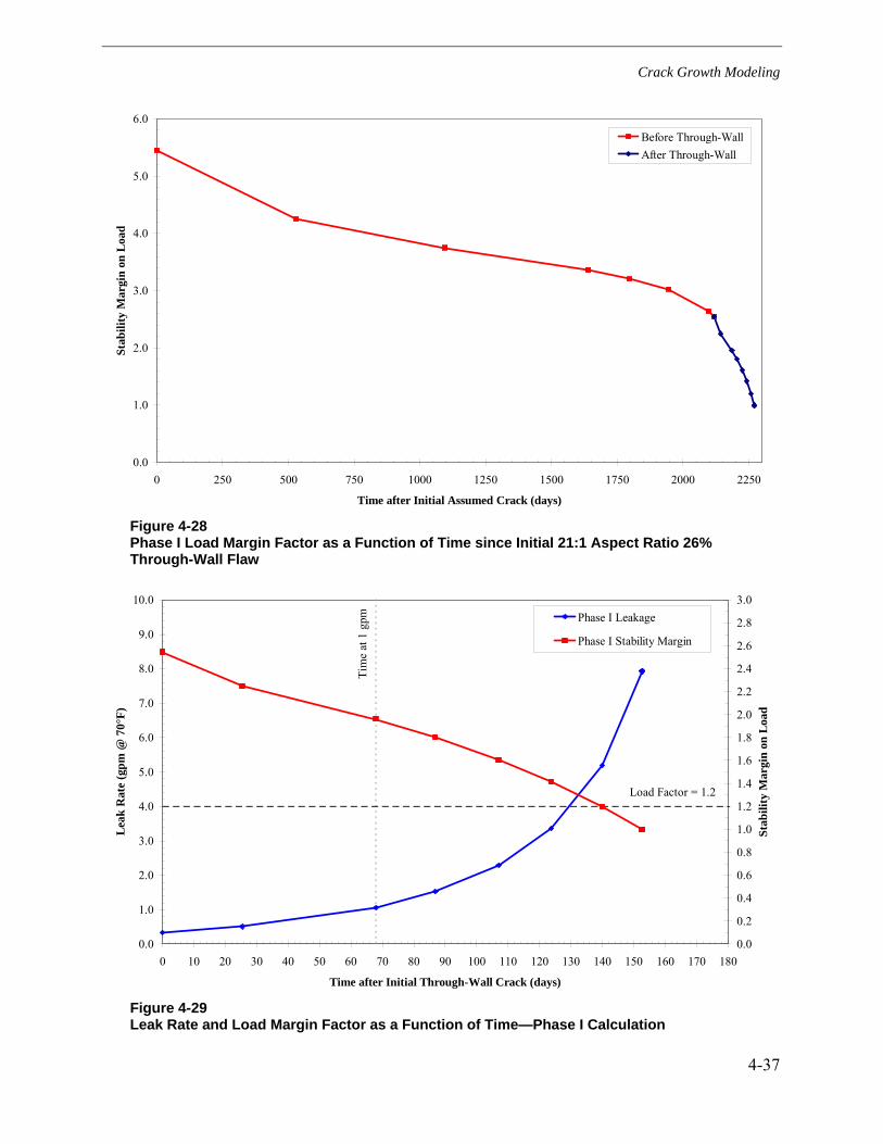
Crack Growth Modeling

4-37

0.0

1.0

2.0

3.0

4.0

5.0

6.0

0 250 500 750 1000 1250 1500 1750 2000 2250

Time after Initial Assumed Crack (days)

Stab

ility

Mar

gin

on L

oad

Before Through-WallAfter Through-Wall

Figure 4-28 Phase I Load Margin Factor as a Function of Time since Initial 21:1 Aspect Ratio 26% Through-Wall Flaw

0.0

1.0

2.0

3.0

4.0

5.0

6.0

7.0

8.0

9.0

10.0

0 10 20 30 40 50 60 70 80 90 100 110 120 130 140 150 160 170 180

Time after Initial Through-Wall Crack (days)

Lea

k R

ate

(gpm

@ 7

0°F)

0.0

0.2

0.4

0.6

0.8

1.0

1.2

1.4

1.6

1.8

2.0

2.2

2.4

2.6

2.8

3.0

Stab

ility

Mar

gin

on L

oad

Phase I Leakage

Phase I Stability Margin

Load Factor = 1.2

Tim

e at

1 g

pm

Figure 4-29 Leak Rate and Load Margin Factor as a Function of Time—Phase I Calculation

Crack Growth Modeling

4-38

0

0.1

0.2

0.3

0.4

0.5

0.6

0.7

0.8

0.9

0 1 2 3 4 5 6 7 8

Surface Crack length (inch)

a/t

alpha=8, a/t=5, c=5alpha=2, a/t=0.8, c=7alpha=5, a/t=0.25, c=1.5Extra Case

-5

-4

-3

-2

-1

0

1

2

3

4

5

0 1 2 3 4 5

alpha=5, a/t=0.25, c=1.5alpha=8, a/t=0.5, c=5alpha=2, a/t=0.8, c=7Extra Case

Figure 4-30 Flaw Profiles Used for Crack Tip SIF Calculation Verification

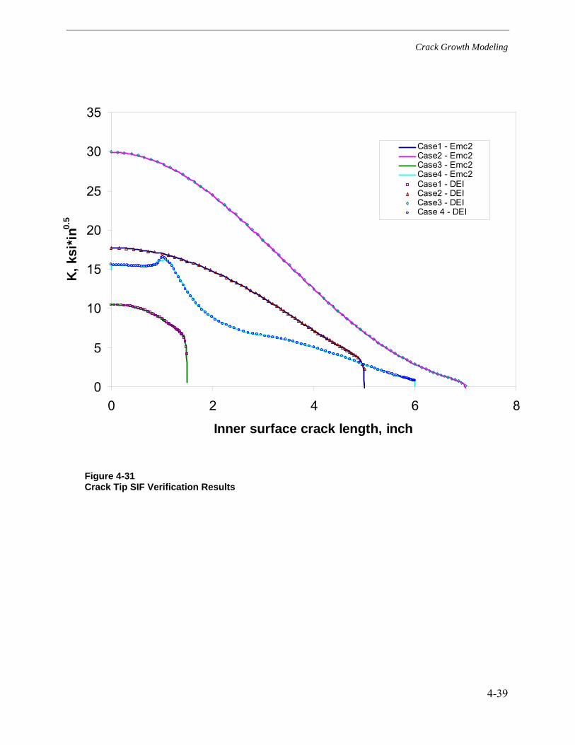
Crack Growth Modeling

4-39

0

5

10

15

20

25

30

35

0 2 4 6 8

Inner surface crack length, inch

K, k

si*i

n0.5

Case1 - Emc2Case2 - Emc2Case3 - Emc2Case4 - Emc2Case1 - DEICase2 - DEICase3 - DEICase 4 - DEI

Figure 4-31 Crack Tip SIF Verification Results

Crack Growth Modeling

4-40

0.0

0.2

0.4

0.6

0.8

1.0

1.2

1.4

0 20 40 60 80 100 120 140 160 180

Angle, θ (deg)

Cra

ck D

epth

, y (i

n)30 Steps - Original Mesh (Base Case)70 Steps - Original Mesh (Temporal Refinement)30 Steps - Refined Mesh (Spatial Refinement)

Figure 4-32 Temporal and Spatial Convergence Results for Case 1 360° Surface Crack Growth Progression

0.0

0.2

0.4

0.6

0.8

1.0

1.2

1.4

0 20 40 60 80 100 120 140 160 180

Angle, θ (deg)

Cra

ck D

epth

, y (i

n)

65 Steps - Original Mesh (Base Case)130 Steps - Original Mesh (Temporal Refinement)65 Steps - Refined Mesh (Spatial Refinement)

Figure 4-33 Temporal and Spatial Convergence Results for Case 1 Complex Crack Growth Progression

Crack Growth Modeling

4-41

Figure 4-34 Cross Section Through 360° Part Depth Crack at Duane Arnold [22]

Crack Growth Modeling

4-42

y = 2091.284192x4 - 4024.030339x3 + 2171.322441x2 - 279.638139x + 4.697888

-50

-40-30

-20-10

0

1020

30

4050

6070

80

0.0 0.2 0.4 0.6 0.8 1.0

Dist from Thermal Sleeve ID (in.)

Axi

al W

RS

(ksi

)Tip of

CreviceThermal Sleeve Safe-End

Figure 4-35 Polynomial Fit to Duane Arnold WRS Finite-Element Analysis Results

Figure 4-36 Comparison of Actual Duane Arnold Crack Profile with Simulated Crack Profile Assuming Initial 30% through-wall 360° Surface Flaw

Actual Crack Profile

Simulated Crack Profile

5-1

5 CRITICAL CRACK SIZE CALCULATIONS

This section describes the development of a conservative critical crack size methodology specific to the subject nozzle-to-safe-end geometry and materials. This methodology is based on the net section collapse (NSC) equations for an arbitrary circumferential crack profile in a thin-walled pipe. For the purposes of this project, normal thermal piping loads were included in the crack stability calculations, and a Z-factor approach reducing the NSC failure load was implemented in consideration of the possibility of an EPFM failure mechanism. Finally, in support of the methodology, available experimental failure data for complex cracks in materials similar to Alloy 82/182 were evaluated.

5.1 Methodology

Critical crack sizes were computed using a spreadsheet implementation of the Net Section Collapse (NSC) solution for an arbitrary circumferential crack profile, assuming thin wall equilibrium [24]. Since crack front coordinates were available for each step of the crack growth simulations, stability calculations could be performed at every increment of crack growth with the net section collapse model. Combined with the leak rate simulations discussed in Section 6, which could also be performed at each increment of through-wall crack growth, evolutions of leak rate and stability margin on load versus time were computed and are presented in Section 7. The NSC solution presented in Reference [24] allows for the calculation of net section collapse loads under three different scenarios. The first is used when the crack is entirely in tension. The second and third scenarios are used when part of the crack is below the cracked section’s neutral axis; the second scenario allows the crack to take compression while the third scenario assumes that the crack cannot take compression. For all calculations in this report, if part of the crack was below the cracked section’s neutral axis, it was conservatively assumed not to take compression.

Given that any hypothetical stress corrosion cracking could be located near the safe end, the flow strength used in the critical crack size calculations was based on the safe end material. Based on design drawings and certified material test report (CMTR) information for the nine plants considered in this analysis, most of the stainless steel safe ends were constructed from SA182 Grade F316L. The remaining safe ends were constructed from SA182 Grade F316 except for the safe ends for the Plant I surge and safety/relief nozzles, which are cast stainless steel SA-351 Grade CF8M. The room-temperature yield and ultimate tensile strengths obtained from the various CMTRs are plotted in Figure 5-1 along with the flow strength calculated as the average of the yield strength and ultimate tensile strength. These were adjusted to a temperature of 650°F based on the relative dependence of yield strength and ultimate tensile strength on temperature in the ASME Boiler & Pressure Vessel Code per Equation [5-1].

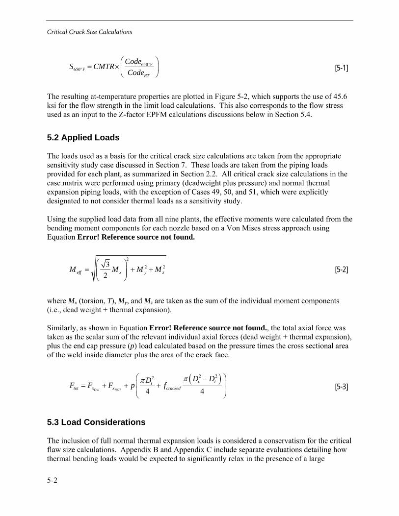
Critical Crack Size Calculations

5-2

650 F650 F

RT

CodeS CMTRCode

°°

⎛ ⎞= ×⎜ ⎟

⎝ ⎠ [5-1]

The resulting at-temperature properties are plotted in Figure 5-2, which supports the use of 45.6 ksi for the flow strength in the limit load calculations. This also corresponds to the flow stress used as an input to the Z-factor EPFM calculations discussions below in Section 5.4.

5.2 Applied Loads

The loads used as a basis for the critical crack size calculations are taken from the appropriate sensitivity study case discussed in Section 7. These loads are taken from the piping loads provided for each plant, as summarized in Section 2.2. All critical crack size calculations in the case matrix were performed using primary (deadweight plus pressure) and normal thermal expansion piping loads, with the exception of Cases 49, 50, and 51, which were explicitly designated to not consider thermal loads as a sensitivity study.

Using the supplied load data from all nine plants, the effective moments were calculated from the bending moment components for each nozzle based on a Von Mises stress approach using Equation Error! Reference source not found.

2

2 232eff x y zM M M M

⎛ ⎞= + +⎜ ⎟⎜ ⎟

⎝ ⎠ [5-2]

where Mx (torsion, T), My, and Mz are taken as the sum of the individual moment components (i.e., dead weight + thermal expansion).

Similarly, as shown in Equation Error! Reference source not found., the total axial force was taken as the scalar sum of the relevant individual axial forces (dead weight + thermal expansion), plus the end cap pressure (p) load calculated based on the pressure times the cross sectional area of the weld inside diameter plus the area of the crack face.

( )2 22

4 4DW NOT

o iitot x x cracked

D DDF F F p fππ⎛ ⎞−

⎜ ⎟= + + +⎜ ⎟⎝ ⎠

[5-3]

5.3 Load Considerations

The inclusion of full normal thermal expansion loads is considered a conservatism for the critical flaw size calculations. Appendix B and Appendix C include separate evaluations detailing how thermal bending loads would be expected to significantly relax in the presence of a large

Critical Crack Size Calculations

5-3

circumferential flaw. Of particular interest are the surge nozzle thermal loads, which generate larger stresses than the thermal loads for the safety/relief and spray nozzles. The Appendix B study reviews test data from the NRC-sponsored Degraded Piping Program and provides analysis results from piping models for the surge lines of two representative plants. The results of this study support the conclusion that the surge nozzle piping thermal loads are completely relieved prior to nozzle rupture since the supportable crack plane rotation is greater than the imposed rotation due to thermal expansion. Appendix C describes a set of elastic and elastic-plastic finite element analyses of a pipe with an idealized through-thickness crack that were used to determine the effect on bending moment and crack driving force due to an imposed end rotation. The analyses performed in Appendix C result in a similar amount of crack plane rotation as the Appendix B results. As discussed in Section 2.2.2, the additional conservatism introduced by including the normal thermal loads bounds the potential effects of potentially higher thermal loads in the surge line during heat and cooldown due to stratification.

Welding residual stresses and through-wall bending stresses caused by radial differential thermal expansion between the stainless steel piping and the carbon steel nozzle were likewise not included as part of the limit load analyses since they are local secondary stresses. Seismic loads were also neglected from the critical crack size calculations since it was considered overly conservative to consider such an unlikely event given the time frame under investigation (~6 months). It should be noted that the loads resulting from an SSE event were not significantly higher than those resulting from the combination of pressure, dead weight, and normal operation thermal.

5.4 EPFM Considerations

Though the crack growth calculations were performed elastically, the critical crack size calculations included elastic-plastic considerations through the use of a Z factor. The Z factor acts as a correction factor on the limit load solution and is a function of the material toughness and pipe diameter. It is used to reduce the supportable moment when elastic-plastic fracture mechanics conditions control rather than limit load conditions. Per Reference [25], for a given material, the Z factor is solely a function of the size of a weld (NPS). For the case of Alloy 82/182, Z factor curves were calculated [26,27] using the stainless steel base metal strength and the toughness of the Alloy 182 weld metal. Fits to the calculation results yielded Equation [5-4].

3 2

3 2

0.00065 0.01386 0.1034 0.902 , 8"0.0000022 0.0002 0.0064 1.1355 , 8"

NPS NPS NPS NPSZ

NPS NPS NPS NPS

⎧ − + + ≤⎪= ⎨− + + >⎪⎩

[5-4]

In this analysis, the Z factor as calculated using Equation [5-4] was used to reduce the supportable moment, thereby reducing the margin on stability for a given crack profile. However, experimental evidence suggests that a Z factor needs only be applied when the Dimensionless Plastic Zone Parameter (DPZP), an empirically based parameter providing a measure of the size of the plastic zone at the crack tip relative to the pipe size (see Section 5.6), is less than unity. In the analyses conducted, a Z factor was conservatively applied to all limit load calculations regardless of the DPZP for the case under consideration.

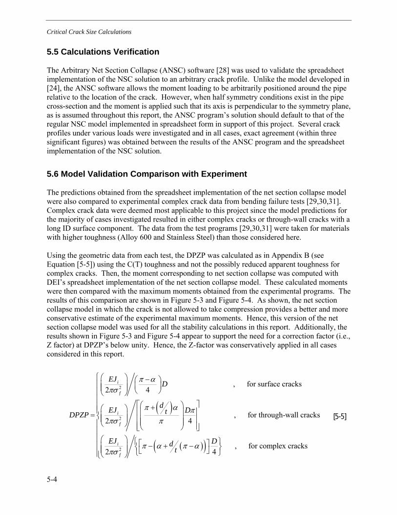
Critical Crack Size Calculations

5-4

5.5 Calculations Verification

The Arbitrary Net Section Collapse (ANSC) software [28] was used to validate the spreadsheet implementation of the NSC solution to an arbitrary crack profile. Unlike the model developed in [24], the ANSC software allows the moment loading to be arbitrarily positioned around the pipe relative to the location of the crack. However, when half symmetry conditions exist in the pipe cross-section and the moment is applied such that its axis is perpendicular to the symmetry plane, as is assumed throughout this report, the ANSC program’s solution should default to that of the regular NSC model implemented in spreadsheet form in support of this project. Several crack profiles under various loads were investigated and in all cases, exact agreement (within three significant figures) was obtained between the results of the ANSC program and the spreadsheet implementation of the NSC solution.

5.6 Model Validation Comparison with Experiment

The predictions obtained from the spreadsheet implementation of the net section collapse model were also compared to experimental complex crack data from bending failure tests [29,30,31]. Complex crack data were deemed most applicable to this project since the model predictions for the majority of cases investigated resulted in either complex cracks or through-wall cracks with a long ID surface component. The data from the test programs [29,30,31] were taken for materials with higher toughness (Alloy 600 and Stainless Steel) than those considered here.

Using the geometric data from each test, the DPZP was calculated as in Appendix B (see Equation [5-5]) using the C(T) toughness and not the possibly reduced apparent toughness for complex cracks. Then, the moment corresponding to net section collapse was computed with DEI’s spreadsheet implementation of the net section collapse model. These calculated moments were then compared with the maximum moments obtained from the experimental programs. The results of this comparison are shown in Figure 5-3 and Figure 5-4. As shown, the net section collapse model in which the crack is not allowed to take compression provides a better and more conservative estimate of the experimental maximum moments. Hence, this version of the net section collapse model was used for all the stability calculations in this report. Additionally, the results shown in Figure 5-3 and Figure 5-4 appear to support the need for a correction factor (i.e., Z factor) at DPZP’s below unity. Hence, the Z-factor was conservatively applied in all cases considered in this report.

( )2

2

2

, for surface cracks2 4

, for through-wall cracks2 4

2

i

f

i

f

i

f

EJ D

dEJ DtDPZP

EJ

π απσ

π α ππσ π

ππσ

⎛ ⎞ −⎛ ⎞⎜ ⎟ ⎜ ⎟⎜ ⎟ ⎝ ⎠⎝ ⎠

⎡ ⎤⎛ ⎞+⎛ ⎞ ⎢ ⎥⎜ ⎟= ⎜ ⎟⎜ ⎟ ⎢ ⎥⎜ ⎟⎜ ⎟⎝ ⎠ ⎢ ⎥⎝ ⎠⎣ ⎦⎛ ⎞

−⎜ ⎟⎜ ⎟⎝ ⎠

( )( ) , for complex cracks4Dd

tα π α

⎧⎪⎪⎪⎪⎪⎨⎪⎪⎪ ⎧ ⎫⎡ ⎤+ −⎪ ⎨ ⎬⎣ ⎦⎩ ⎭⎪⎩

[5-5]

Critical Crack Size Calculations

5-5

0

10

20

30

40

50

60

70

80

90

100

01 A

- R

e (7

.75x

5.17

)

02 A

- S

A (7

.75x

5.17

)

03 A

- S

B (7

.75x

5.17

)

04 A

- S

C (7

.75x

5.17

)

05 E

- R

e (7

.75x

5.17

)

06 E

- S

A (7

.75x

5.17

)

07 E

- S

B (7

.75x

5.17

)

08 E

- S

C (7

.75x

5.17

)

09 H

- R

e (7

.75x

5.17

)

10 H

- S

A (7

.75x

5.17

)

11 H

- S

B (7

.75x

5.17

)

12 H

- S

C (7

.75x

5.17

)

WC

1 J

- Re

(7.7

5x5.

17)

14 F

- S

A (8

x5.1

9)

15 F

- S

B (8

x5.1

9)

16 F

- S

C (8

x5.1

9)

17 B

- R

e (7

.75x

5.62

)

18 B

- S

A (7

.75x

5.62

)

19 B

- S

B (7

.75x

5.62

)

20 B

- S

C (7

.75x

5.62

)

21 G

- R

e (7

.75x

5.62

)

22 G

- S

A (7

.75x

5.62

)

23 G

- S

B (7

.75x

5.62

)

24 G

- S

C (7

.75x

5.62

)

25 C

- R

e (7

.75x

5.62

)

26 C

- S

A (7

.75x

5.62

)

27 C

- S

B (7

.75x

5.62

)

28 C

- S

C (7

.75x

5.62

)

29 D

- R

e (8

x4.9

37)

30 D

- S

A (8

x4.9

37)

31 D

- S

B (8

x4.9

37)

32 D

- S

C (8

x4.9

37)

33 I

- Re

(8x4

.937

)

34 I

- SA

(8x4

.937

)

35 I

- SB

(8x4

.937

)

36 A

- S

p (5

.81x

4.01

)

37 E

- S

p (5

.81x

4.01

)

WC

5 J

- Sp

(5.8

1x4.

01)

39 G

- S

p (5

.81x

4.25

)

40 C

- S

p (5

.81x

4.25

)

41 F

- S

p (8

x5.6

95)

42 D

- S

p (5

.188

x3.0

62)

43 I

- Sp

(5.1

88x3

.25)

44 A

- S

u (1

5x11

.844

)

45 E

- S

u (1

5x11

.844

)

46 H

- S

u (1

5x11

.844

)

WC

6 J

- Su

(15x

11.8

44)

48 G

- S

u (1

5x11

.844

)

49 C

- S

u (1

5x11

.875

)

50 D

- S

u (1

3.06

3x10

.125

)

51 I

- Su

(13.

063x

10.1

25)

CM

TR S

afe

End

Stre

ngth

Val

ues

(ksi

)

0

0.1

0.2

0.3

0.4

0.5

0.6

0.7

0.8

0.9

1

0.00

0.50

1.00

1.50

2.00

2.50

3.00

4.75

5.25

5.75

6.25

6.75

7.25

7.75

8.25

8.75

9.25

9.75

10.2

5

11.0

0

11.5

0

12.0

0

12.5

0

13.0

0

13.7

5

14.2

5

14.7

5

15.2

5

15.7

5

16.2

5

16.7

5

17.2

5

17.7

5

18.2

5

18.7

5

19.2

5

19.7

5

20.2

5

20.7

5

21.2

5

21.7

5

22.2

5

22.7

5

23.2

5

23.7

5

24.2

5

24.7

5

25.2

5

25.7

5

26.2

5

26.7

5

27.2

5

27.7

5

28.2

5

28.7

5

29.2

5

29.7

5

30.2

5

30.7

5

31.2

5

31.7

5

32.2

5

32.7

5

33.2

5

33.7

5

34.2

5

34.7

5

35.2

5

35.7

5

36.2

5

36.7

5

37.2

5

37.7

5

38.2

5

38.7

5

39.2

5

39.7

5

40.2

5

40.7

5

41.2

5

41.7

5

42.2

5

42.7

5

43.2

5

43.7

5

44.2

5

44.7

5

45.2

5

45.7

5

46.2

5

46.7

5

47.2

5

47.7

5

48.2

5

48.7

5

49.2

5

49.7

5

50.2

5

50.7

5

51.2

5

51.7

5

52.2

5

52.7

5

53.2

5

53.7

5

54.2

5

54.7

5

55.2

5

55.7

5

56.2

5

56.7

5

57.2

5

57.7

5

58.2

5

58.7

5

59.2

5

59.7

5

CMTR UTSCMTR FSCMTR YS

Flow strength (FS) taken as average of YS and UTS listed in safe end CMTR.

Figure 5-1 Available CMTR Strength Data for Subject Stainless Steel Safe Ends

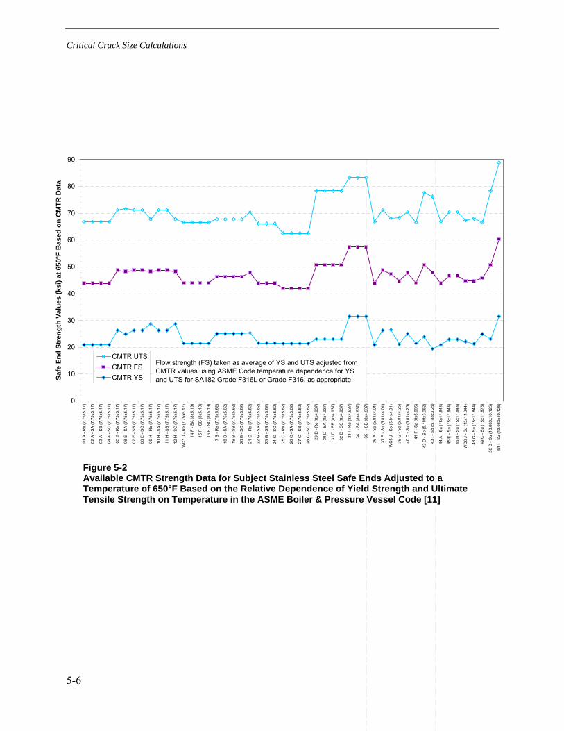
Critical Crack Size Calculations

5-6

0

10

20

30

40

50

60

70

80

90

01 A

- R

e (7

.75x

5.17

)

02 A

- S

A (7

.75x

5.17

)

03 A

- S

B (7

.75x

5.17

)

04 A

- S

C (7

.75x

5.17

)

05 E

- R

e (7

.75x

5.17

)

06 E

- S

A (7

.75x

5.17

)

07 E

- S

B (7

.75x

5.17

)

08 E

- S

C (7

.75x

5.17

)

09 H

- R

e (7

.75x

5.17

)

10 H

- S

A (7

.75x

5.17

)

11 H

- S

B (7

.75x

5.17

)

12 H

- S

C (7

.75x

5.17

)

WC

1 J

- Re

(7.7

5x5.

17)

14 F

- S

A (8

x5.1

9)

15 F

- S

B (8

x5.1

9)

16 F

- S

C (8

x5.1

9)

17 B

- R

e (7

.75x

5.62

)

18 B

- S

A (7

.75x

5.62

)

19 B

- S

B (7

.75x

5.62

)

20 B

- S

C (7

.75x

5.62

)

21 G

- R

e (7

.75x

5.62

)

22 G

- S

A (7

.75x

5.62

)

23 G

- S

B (7

.75x

5.62

)

24 G

- S

C (7

.75x

5.62

)

25 C

- R

e (7

.75x

5.62

)

26 C

- S

A (7

.75x

5.62

)

27 C

- S

B (7

.75x

5.62

)

28 C

- S

C (7

.75x

5.62

)

29 D

- R

e (8

x4.9

37)

30 D

- S

A (8

x4.9

37)

31 D

- S

B (8

x4.9

37)

32 D

- S

C (8

x4.9

37)

33 I

- Re

(8x4

.937

)

34 I

- SA

(8x4

.937

)

35 I

- SB

(8x4

.937

)

36 A

- S

p (5

.81x

4.01

)

37 E

- S

p (5

.81x

4.01

)

WC

5 J

- Sp

(5.8

1x4.

01)

39 G

- S

p (5

.81x

4.25

)

40 C

- S

p (5

.81x

4.25

)

41 F

- S

p (8

x5.6

95)

42 D

- S

p (5

.188

x3.0

62)

43 I

- Sp

(5.1

88x3

.25)

44 A

- S

u (1

5x11

.844

)

45 E

- S

u (1

5x11

.844

)

46 H

- S

u (1

5x11

.844

)

WC

6 J

- Su

(15x

11.8

44)

48 G

- S

u (1

5x11

.844

)

49 C

- S

u (1

5x11

.875

)

50 D

- S

u (1

3.06

3x10

.125

)

51 I

- Su

(13.

063x

10.1

25)

Safe

End

Str

engt

h Va

lues

(ksi

) at 6

50°F

Bas

ed o

n C

MTR

Dat

a

0

0.1

0.2

0.3

0.4

0.5

0.6

0.7

0.8

0.9

10.0

00.7

51.5

02.2

53.0

05.0

05.7

56.5

07.2

58.0

08.7

59.5

010

.2511

.2512

.0012

.7513

.7514

.5015

.2516

.0016

.7517

.5018

.2519

.0019

.7520

.5021

.2522

.0022

.7523

.5024

.2525

.0025

.7526

.5027

.2528

.0028

.7529

.5030

.2531

.0031

.7532

.5033

.2534

.0034

.7535

.5036

.2537

.0037

.7538

.5039

.2540

.0040

.7541

.5042

.2543

.0043

.7544

.5045

.2546

.0046

.7547

.5048

.2549

.0049

.7550

.5051

.2552

.0052

.7553

.5054

.2555

.0055

.7556

.5057

.2558

.0058

.7559

.50

CMTR UTSCMTR FSCMTR YS

Flow strength (FS) taken as average of YS and UTS adjusted from CMTR values using ASME Code temperature dependence for YS and UTS for SA182 Grade F316L or Grade F316, as appropriate.

Figure 5-2 Available CMTR Strength Data for Subject Stainless Steel Safe Ends Adjusted to a Temperature of 650°F Based on the Relative Dependence of Yield Strength and Ultimate Tensile Strength on Temperature in the ASME Boiler & Pressure Vessel Code [11]

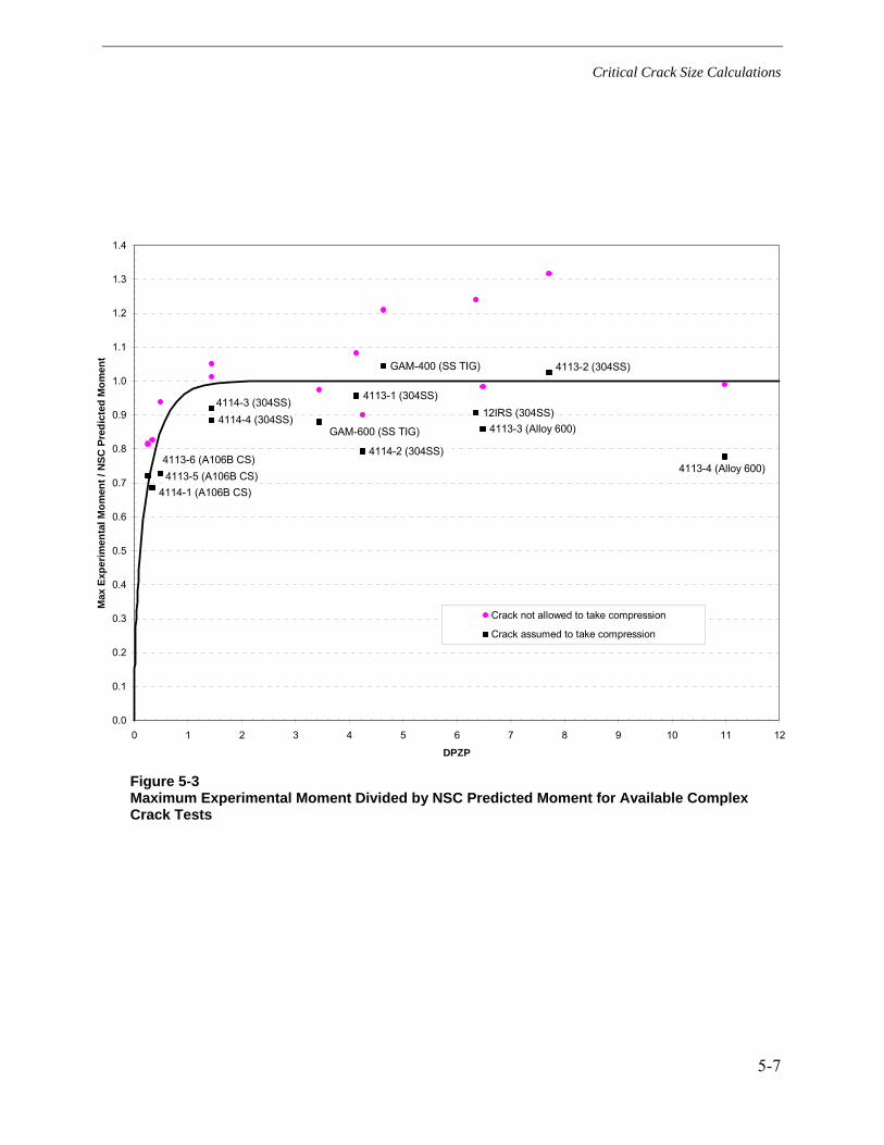
Critical Crack Size Calculations

5-7

4113-4 (Alloy 600)

4113-3 (Alloy 600)12IRS (304SS)

GAM-400 (SS TIG)

4113-1 (304SS)

4114-2 (304SS)

GAM-600 (SS TIG)4114-4 (304SS)

4113-2 (304SS)

4114-3 (304SS)

4114-1 (A106B CS)4113-5 (A106B CS)4113-6 (A106B CS)

0.0

0.1

0.2

0.3

0.4

0.5

0.6

0.7

0.8

0.9

1.0

1.1

1.2

1.3

1.4

0 1 2 3 4 5 6 7 8 9 10 11 12

DPZP

Max

Exp

erim

enta

l Mom

ent /

NSC

Pre

dict

ed M

omen

t

Crack not allowed to take compression

Crack assumed to take compression

Figure 5-3 Maximum Experimental Moment Divided by NSC Predicted Moment for Available Complex Crack Tests

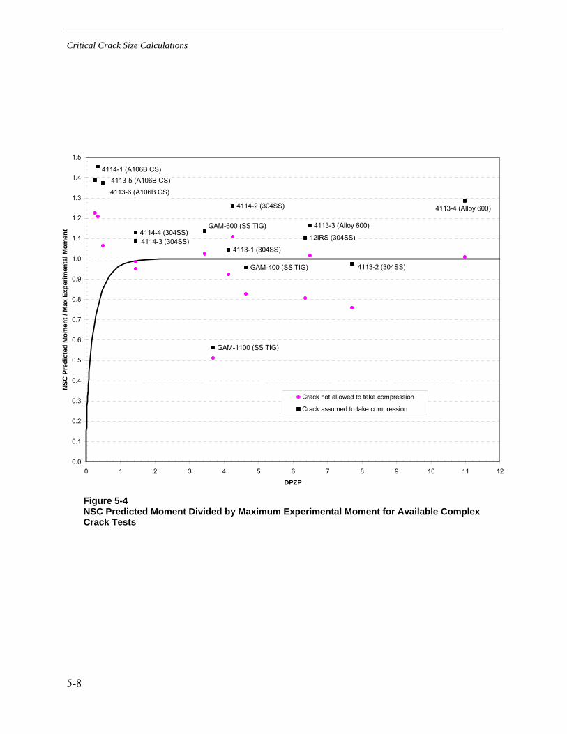
Critical Crack Size Calculations

5-8

GAM-1100 (SS TIG)

4113-4 (Alloy 600)

4113-3 (Alloy 600)

12IRS (304SS)

GAM-400 (SS TIG)

4113-1 (304SS)

4114-2 (304SS)

GAM-600 (SS TIG)4114-4 (304SS)

4113-2 (304SS)

4114-3 (304SS)

4114-1 (A106B CS)4113-5 (A106B CS)

4113-6 (A106B CS)

0.0

0.1

0.2

0.3

0.4

0.5

0.6

0.7

0.8

0.9

1.0

1.1

1.2

1.3

1.4

1.5

0 1 2 3 4 5 6 7 8 9 10 11 12

DPZP

NSC

Pre

dict

ed M

omen

t / M

ax E

xper

imen

tal M

omen

t

Crack not allowed to take compression

Crack assumed to take compression

Figure 5-4 NSC Predicted Moment Divided by Maximum Experimental Moment for Available Complex Crack Tests

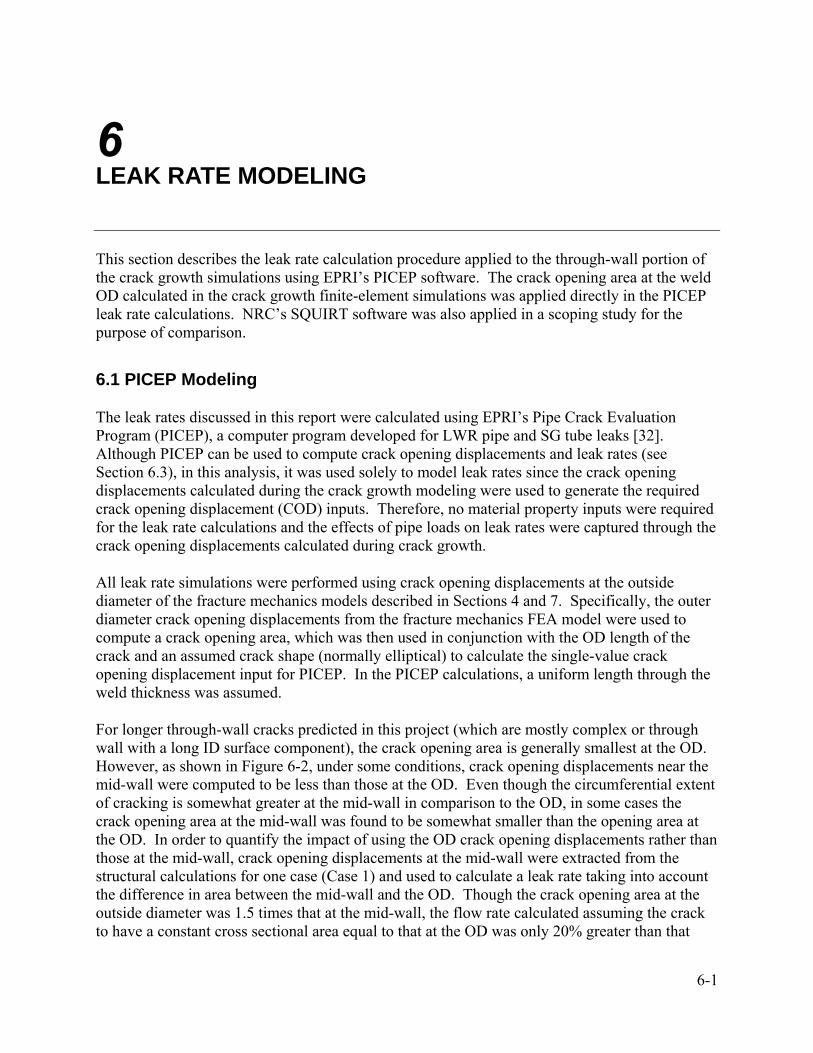
6-1

6 LEAK RATE MODELING

This section describes the leak rate calculation procedure applied to the through-wall portion of the crack growth simulations using EPRI’s PICEP software. The crack opening area at the weld OD calculated in the crack growth finite-element simulations was applied directly in the PICEP leak rate calculations. NRC’s SQUIRT software was also applied in a scoping study for the purpose of comparison.

6.1 PICEP Modeling

The leak rates discussed in this report were calculated using EPRI’s Pipe Crack Evaluation Program (PICEP), a computer program developed for LWR pipe and SG tube leaks [32]. Although PICEP can be used to compute crack opening displacements and leak rates (see Section 6.3), in this analysis, it was used solely to model leak rates since the crack opening displacements calculated during the crack growth modeling were used to generate the required crack opening displacement (COD) inputs. Therefore, no material property inputs were required for the leak rate calculations and the effects of pipe loads on leak rates were captured through the crack opening displacements calculated during crack growth.

All leak rate simulations were performed using crack opening displacements at the outside diameter of the fracture mechanics models described in Sections 4 and 7. Specifically, the outer diameter crack opening displacements from the fracture mechanics FEA model were used to compute a crack opening area, which was then used in conjunction with the OD length of the crack and an assumed crack shape (normally elliptical) to calculate the single-value crack opening displacement input for PICEP. In the PICEP calculations, a uniform length through the weld thickness was assumed.

For longer through-wall cracks predicted in this project (which are mostly complex or through wall with a long ID surface component), the crack opening area is generally smallest at the OD. However, as shown in Figure 6-2, under some conditions, crack opening displacements near the mid-wall were computed to be less than those at the OD. Even though the circumferential extent of cracking is somewhat greater at the mid-wall in comparison to the OD, in some cases the crack opening area at the mid-wall was found to be somewhat smaller than the opening area at the OD. In order to quantify the impact of using the OD crack opening displacements rather than those at the mid-wall, crack opening displacements at the mid-wall were extracted from the structural calculations for one case (Case 1) and used to calculate a leak rate taking into account the difference in area between the mid-wall and the OD. Though the crack opening area at the outside diameter was 1.5 times that at the mid-wall, the flow rate calculated assuming the crack to have a constant cross sectional area equal to that at the OD was only 20% greater than that

Leak Rate Modeling

6-2

calculated using the crack with variable cross sectional area. Given that this effect is considerably smaller than the expected accuracy of the leak rate simulations, the more readily available outside diameter crack opening displacements were used to compute the leak rates in Tables 7-3 and 7-4. No comparisons were made using crack opening displacements at the inside diameter since, as stated earlier, most cases exhibited either complex cracks or through-wall cracks with long ID surface components leading to even larger crack opening areas than those at the outside diameter.

The inputs to the leak rate calculations are listed in Table 6-1. The fluid flow parameters were selected to be representative of flow through PWSCC cracks [32,33]. The results of the leak rate simulations are included with the stability results in Tables 7-3 and 7-4.

6.2 Scoping Results

As part of the leakage calculations, scoping analyses were performed to confirm the appropriate selection of inputs. Specifically, the effect of assuming the crack shape to be elliptical was investigated. The choice of an elliptical shape was motivated by the actual crack opening displacements computed during the crack growth simulations. A plot showing the shape of the crack opening at the OD for Case 1 when the leak rate was calculated to be 1 gpm is shown in Figure 6-3 along with the elliptical, diamond, and rectangular profiles which correspond to the actual profile’s crack opening area and length. As seen in the figure, the actual shape of the crack is very well approximated by an ellipse.

In order to quantify the effect of assumed crack shape, leakage simulations were conducted for one case using rectangular and diamond shaped crack openings rather than the default ellipse. The results showed the ellipse to be conservative (i.e., result in lower flow rate) by 2% relative to the other two crack shapes. Therefore, the elliptical crack shape was used to generate all of the leak rate results shown in Tables 7-3 and 7-4.

6.3 Comparison with SQUIRT Modeling

As part of leakage calculation verification studies, comparisons were made between leak rates predicted using PICEP and those predicted using the NRC’s Seepage Quantification of Upsets in Reactor Tubes (SQUIRT) program [34]. Since these calculations were performed prior to the crack growth calculations, a slightly different approach than that described in Section 6.1 was used. Specifically, PICEP was used to calculate both crack opening displacement and leakage for a given crack length, loading condition, and assumed crack shape. A summary of the structural inputs used in the crack opening displacement calculations is provided in Table 6-2. The crack opening displacement and assumed crack shape were then used to calculate the leak rate using the SQUIRT code for the same assumed crack shape.

When specifying the crack geometry, PICEP allows the user to vary the crack opening area linearly from the ID to the OD whereas SQUIRT allows the user to linearly vary the crack length and opening independently through the thickness. In order to be compatible with the inputs used in PICEP, the crack length and opening used in SQUIRT were kept constant through the

Leak Rate Modeling

6-3

thickness resulting in a constant crack cross-sectional area through the thickness. The assumed crack shape for this study was taken to be rectangular. As described in Section 6.2, the shape of the crack was concluded to have a minimal effect on the predicted leak rates.

The PICEP modeling used the same fluid friction inputs as those used in the final leakage calculations presented in Tables 7-3 and 7-4. The SQUIRT simulations were conducted using its built-in PWSCC modeling inputs.

The leak rate calculations were done for cracks ranging in length from 1 to 10 inches using the geometry and loading applicable to the Wolf Creek relief nozzle, and the results are shown in Figure 6-1. As shown in the figure, the PICEP calculations spanned a range of applied bending moments, whereas the SQUIRT calculations were performed only for the full moment case. It is clear from the figure that the leak rates obtained using the SQUIRT code, albeit consistently greater than those obtained using PICEP (1% to 30% greater in the figure), are generally in good agreement with those obtained from PICEP. The results in Figure 6-1 also clearly demonstrate the effect of the applied bending moment to increase the crack opening area and, thus, leak rate.

6.4 Leak Rate Predication Uncertainty

An estimate of the uncertainty associated with the leak rate calculations described above is presented in Appendix D of this report. This appendix describes a statistical study of experimental leak rate data for through-wall cracks having an IGSCC morphology. The study shows that a multiplicative factor of 1.5 to 2.0 on the leak rate calculated using the NRC SQUIRT code describes the uncertainty in leak rate due to scatter in the test data for the IGSCC samples tested. As noted in Section 7.2.3, a leak rate margin factor of 4.0 is applied in recognition of other sources of uncertainty in the leak rate calculation not addressed by this statistical evaluation such as the variability in the PWSCC crack morphology parameters (e.g., crack surface roughness and tortuosity) versus the PWSCC type assumptions described in this section.

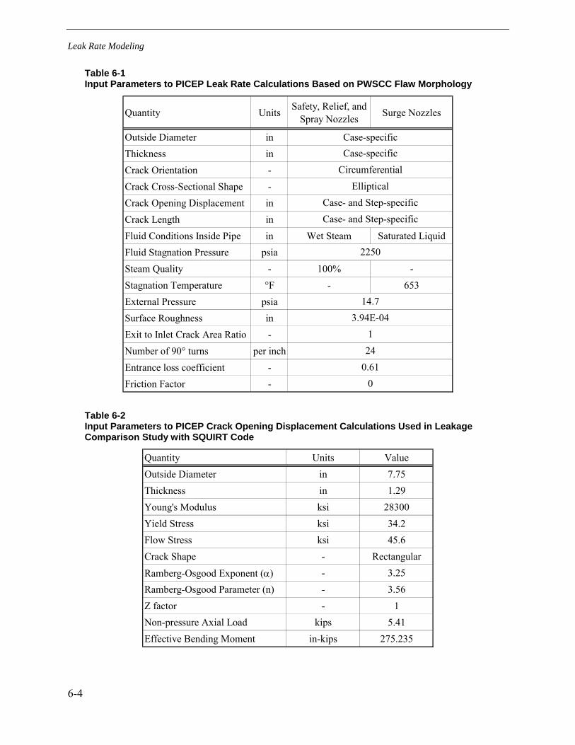
Leak Rate Modeling

6-4

Table 6-1 Input Parameters to PICEP Leak Rate Calculations Based on PWSCC Flaw Morphology

Quantity Units Safety, Relief, and Spray Nozzles Surge Nozzles

Outside Diameter inThickness inCrack Orientation -Crack Cross-Sectional Shape -Crack Opening Displacement inCrack Length inFluid Conditions Inside Pipe in Wet Steam Saturated LiquidFluid Stagnation Pressure psiaSteam Quality - 100% -Stagnation Temperature °F - 653External Pressure psiaSurface Roughness inExit to Inlet Crack Area Ratio -Number of 90° turns per inchEntrance loss coefficient -Friction Factor - 0

EllipticalCircumferentialCase-specificCase-specific

14.7

2250

Case- and Step-specificCase- and Step-specific

0.61241

3.94E-04

Table 6-2 Input Parameters to PICEP Crack Opening Displacement Calculations Used in Leakage Comparison Study with SQUIRT Code

Quantity Units ValueOutside Diameter in 7.75Thickness in 1.29Young's Modulus ksi 28300Yield Stress ksi 34.2Flow Stress ksi 45.6Crack Shape - Rectangular

Ramberg-Osgood Exponent (α) - 3.25Ramberg-Osgood Parameter (n) - 3.56Z factor - 1Non-pressure Axial Load kips 5.41Effective Bending Moment in-kips 275.235

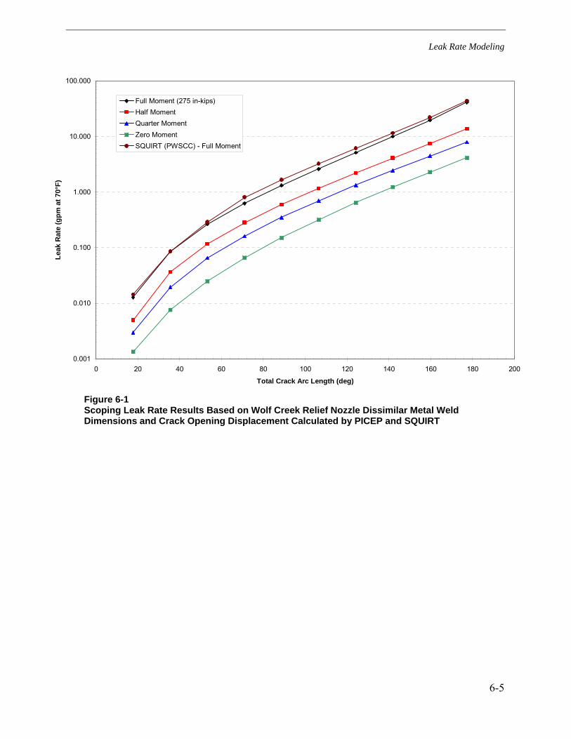
Leak Rate Modeling

6-5

0.001

0.010

0.100

1.000

10.000

100.000

0 20 40 60 80 100 120 140 160 180 200

Total Crack Arc Length (deg)

Leak

Rat

e (g

pm a

t 70°

F)

Full Moment (275 in-kips)Half MomentQuarter MomentZero MomentSQUIRT (PWSCC) - Full Moment

Figure 6-1 Scoping Leak Rate Results Based on Wolf Creek Relief Nozzle Dissimilar Metal Weld Dimensions and Crack Opening Displacement Calculated by PICEP and SQUIRT

Leak Rate Modeling

6-6

ANSYS 10.0A1JUL 2 200717:32:32PLOT NO. 18NODAL SOLUTIONSTEP=1SUB =1TIME=1UZRSYS=11DMX =.003036SEPC=17.667SMN =-.155E-05SMX =.003036

MN

MX

X

Y

Z

-.155E-05.336E-03.673E-03.001011.001348.001686.002023.002361.002698.003036

Case 12 – 1 gpm leak rate

ANSYS 10.0A1JUL 2 200717:33:53PLOT NO. 34NODAL SOLUTIONSTEP=1SUB =1TIME=1UZRSYS=11DMX =.006319SEPC=18.074SMN =-.165E-04SMX =.006319

MN

MX

X

Y

Z

-.165E-04.687E-03.001391.002095.002799.003503.004207.004911.005615.006319

Case 12 – Critical for 1.2 Load Margin Factor Figure 6-2 Crack Opening Displacement Contours for Example Case (Actual COD is Twice Shown Because of Symmetry Condition)

Figure 6-3 Example of Crack Opening Shape on Weld OD

0.000

0.001

0.002

0.003

0.004

0.005

0.006

0.0 0.5 1.0 1.5 2.0 2.5Circumferential Location along OD (in)

Cra

ck O

peni

ng D

ispl

acem

ent (

in)

Crack Opening ProfileDiamondRectangularEllipse

Case 1 at 1 gpm leak rate

PRELIMINARY

7-1

7 SENSITIVITY CASE MATRIX

This section discusses the development and application of an extensive crack growth sensitivity matrix covering the geometry, load, and fabrication factors for each of the 51 subject welds, as well as the uncertainty in key modeling parameters such as those associated with welding residual stress, initial crack shape and depth, the K-dependence of the crack growth rate equation, and the effect of multiple flaw initiation sites in a single weld. Section 7 also presents a set of evaluation criteria that was developed to guide interpretation of the matrix results. The evaluation criteria provide safety margins based on explicit consideration of leak rate detection sensitivity, plant response time, and uncertainty in the crack stability calculations. This section begins with a description of the key modeling outputs that are developed using the crack growth (Section 4), crack stability (Section 5), and leak rate (Section 6) models described in previous sections.

7.1 Modeling Procedure and Outputs

In order to evaluate each crack growth sensitivity case, the following general procedure was applied based on the crack growth, crack stability, and leak rate submodels described in the previous sections:

• Step 1. Using FEACrack, the assumed initial crack is grown as a part-depth surface crack until the crack reaches a depth of about 93% of the wall thickness. This is the maximum depth for which the surface crack can be reliably meshed. In the case of partial-arc surface cracks, if the ends of the crack are calculated to join up, then the partial-arc model is transitioned to a 360° surface crack by assuming that the relatively small ligament between the ends of the partial-arc crack is instantaneously eliminated. In some cases, the surface crack may be observed to arrest prior to growing through-wall due to decay in the driving stress intensity factor to zero. In such cases, the analysis case is terminated at this step.

• Step 2. The surface crack profile is extended from the 93% depth to 100% depth based on a single step using the stress intensity factors along the crack front at the 93% depth.

• Step 3. The final 100% deep surface crack, which intersects the OD surface at a single point, is converted to an initial through-wall or complex crack by eliminating the thin ligament between the final surface crack and the OD surface. It is assumed that this surface ligament between the final 100% deep surface crack and the weld OD is instantaneously cracked in the region in which it is thinner than about 10% of the wall thickness. (In some cases, the surface ligament is assumed to be instantaneously cracked out to a significantly thicker ligament location.) For the case of surge nozzles the initial through-wall total opening angle was typically about 26°, while for the safety/relief and spray nozzles the initial through-wall

Sensitivity Case Matrix

7-2

total opening angle was typically about 42°. However, for the ID repair cases the initial through-wall total opening angle was often about 20° because of the difference in ligament geometry specific to the repair cases.

• Step 4. Using FEACrack, the initial through-wall or complex crack profile from Step 3 is grown until the point that subsequent post-processing shows the crack to reach its stability limit. In a few cases in which the initial through-wall crack is much longer on the inside surface than on the outside surface (e.g., 180° compared to 40°), the initial through-wall crack may be converted to a complex crack because of the difficulty in properly meshing the highly slanted through-wall crack geometry. This was applied in the following cases: 28b, 37c, 38c, 39c, 40c, and 41c. This conversion is a conservative assumption given that the complex crack envelopes the through-wall crack, reducing crack stability while not having a significant effect on the calculated leak rate.

• Step 5. The crack stability load margin factor and leak rate are determined for various steps in the through-wall or complex crack progression as a post-processing calculation as described in Sections 5 and 6. In the crack stability model, the crack face pressure is applied as an increase in the axial end cap load. The total axial load considers the operating pressure acting on the inside diameter cross section and on the crack face, as well as the dead weight and normal operating piping thermal constraint axial forces. Note that in the crack stability calculation the sum of dead weight and normal thermal axial forces is always taken based on the maximum reported for each geometry configuration, even though the typical (i.e., midrange) axial stress is usually assumed in the crack growth calculations. This approach is conservative because a higher axial load will always lead to reduced crack stability, whereas the effect of the axial load magnitude on the overall analysis through its effect on crack growth was not known with certainty before the matrix was substantially completed.

Step 5 facilitates calculating the time from detectable leakage to rupture based on different choices for margin factors on the calculated leak rate and on the loads used to calculate crack stability. Closely related to this time interval output are the calculated leak rates at the beginning and end of this interval. In some cases, the initial leak rate upon cracking of the thin surface ligament between the final surface flaw and OD surface may be greater than the detectable leak rate, including consideration of a margin factor applied to the calculated leak rate. Another key output is the load stability margin factor at the time that the leaking flaw produces a detectable level of leakage. A secondary key output parameter is the time from the initial assumed surface flaw until stable through-wall penetration, or alternatively until rupture. This time may be compared to the operating age of the subject weld as a secondary evaluation.

7.2 Evaluation Criteria

7.2.1 Introduction

In order to facilitate interpretation of the main analysis results of this study, a set of evaluation criteria were developed based on input from the EPRI expert panel and industry representatives. Consideration was given to the many modeling uncertainties addressed in the detailed

Sensitivity Case Matrix

7-3

calculations performed, with explicit treatment of uncertainties in the crack stability and leak rate calculations. Attributes related to RCS leak rate detection sensitivity and plant response times were derived from current licensing commitments of the subject plants.

Hence, analytical case results of this study that meet these evaluation criteria fulfill the objective of this project as stated in Section 1.2 by demonstrating the viability of leakage detection to preclude the potential for rupture. However, these results should be applied by others to make a final determination regarding the timing of the initial PDI examination or mitigation for each of the subject welds.

7.2.2 Criteria

Figure 7-1 illustrates the evaluation criteria that were developed from the calculated development of increasing leak rate and decreasing stability margin with time for the through-wall phase of the crack growth progression. The criteria can be stated in either of two equivalent ways:

1. Are there at least 7 days after the calculated leak rate reaches 1.0 gpm prior to the critical crack size being reached based on a margin factor of 1.2 applied to the applicable loads?

or equivalently

2. Is the crack stability margin factor on the applicable loads at least 1.2 at a time seven days after the calculated leak rate reaches 1.0 gpm?

In Figure 7-1, the line with square markers reflects the calculated leak rate for the predicted through-wall crack as a function of time. The line with circular markers reflects the ratio of the critical supportable load versus the reported operating load (i.e., stability load margin) for the cracked nozzle weld also as a function of time. The plot begins at the time of the initial leaking through-wall crack. Applying a margin factor of four to a detection limit of 0.25 gpm accounts for the analytical uncertainties in calculating the leak rate, and results in a value of 1.0 gpm. Where the leak rate curve intersects 1.0 gpm establishes the beginning time when the hypothetical plant initially identifies the existence of this small leak and initiates its actions in response to a potential unidentified leak source. Conservatively, the plant would be in Mode 5 within the seven day period. The final criterion evaluates the stability margin on load. This is graphically illustrated by plotting a stability margin value of 1.2 on the seven-day line previously established and determining where the stability curve resides relative to this point. If this point is below the stability curve, then plant shutdown prior to rupture is indicated.

7.2.3 Basis

The technical basis for the evaluation criteria are as follows:

• Seven days are conservatively required for the plant to shut down in response to a slowly increasing leak rate after it reaches 0.25 gpm more than the baseline leak rate. In early 2007 US PWRs committed to implement enhanced leakage monitoring programs until completion of inspection / mitigation actions on their pressurizer nozzles. These commitments include

Sensitivity Case Matrix

7-4

daily measurement of RCS leakage and specific timetables for plant actions to identify and respond to a change in RCS leakage relative to a baseline value. The baseline leakage for each plant is established using leak rates measured within 7 days after achieving Mode 1 100% power operation following the most recent bare metal visual examination of the pressurizer Alloy 82/182 butt weld locations. Two leakage thresholds were established: a 0.25 gpm leak rate above the plant baseline that is sustained for 72 hours; or a 0.1 gpm leak rate change from one day to the next, which is sustained for 72 hours. If either of these thresholds is exceeded, and it cannot be confirmed that it is from sources other than pressurizer nozzle welds, then the unit will be placed in Mode 3 within 6 hours and Mode 5 within 36 hours. Therefore, the cumulative total elapsed time, assuming that a through-wall leak occurs just after the daily leakage measurement, would be approximately 6 days. However, because key actions in this sequence occur on roughly a daily basis, an additional full day has been included to conservatively define a minimum plant response period for application within the evaluation criteria.

• A margin factor of 4.0 is applied to a level of leakage (0.25 gpm) that plant detection systems can confidently detect to account for uncertainty in the calculated leak rate. A statistical study comparing the predictions of the SQUIRT leak rate code to leak rate measurements for IGSCC samples (see Appendix D) shows that for measured leak rates greater than about 0.1 gpm, there is a 95% probability that the predicted leak rate is within a factor of 1.5 to 2.0 of the measured value. The EPRI PICEP code, which was used in this study to calculate the leak rate for the matrix of crack growth sensitivity cases, conservatively tends to predict a slightly lower leak rate compared to the SQUIRT code given the modeling inputs appropriate to PWSCC presented in Section 6. The final leak rate margin factor of 4.0 is applied in recognition of other sources of uncertainty in the leak rate calculation not addressed by the statistical evaluation cited above such as the variability in the PWSCC crack morphology parameters (e.g., crack surface roughness and tortuosity) versus the PWSCC type assumptions in Section 6. This margin factor is also judged adequate to account for any delayed plant response that might result if sustained daily average leakage declines below the defined baseline leakage. However, to place normal plant RCS unidentified leakage in context, typical baseline leakage rates within several of the subject plants reported in a recent informal poll were on the order of 0.1 gpm or less.

• The margin factor of 1.2 on the loads applied in the critical crack size calculation accounts for uncertainty in these loads and in the critical crack size calculation methodology. The stability margin factor is the factor that when multiplied with each of the nozzle load components results in the critical loading that produces crack instability and rupture. The factor of 1.2 is appropriate in consideration of the significant conservatisms implemented in the critical crack size calculation methodology of Section 5. First, the secondary normal operating piping thermal constraint loads are included in the critical crack size calculation on an equal basis with the primary pressure and dead weight loads, although evaluations tend to demonstrate that such secondary loads are expected to be significantly or completely relaxed prior to failure. Second, the critical supportable load is reduced using a Z-factor approach to account for the possibility of an EPFM failure mechanism, although there is no clear evidence that a purely limit load based approach is insufficient. (It is recognized that there are no experimental data specific to circumferential cracks in Alloy 82/182 piping butt welds verifying that limit load rather than elastic-plastic fracture conditions control for this specific

Sensitivity Case Matrix

7-5

material.) Third, the safe end strength properties are applied in the critical crack size calculation. This has been shown to be appropriate for cracks located close to the safe end material. However, the WRS simulations tend to show that the highest axial stresses are located toward or within the butter weld material built up on the low alloy steel nozzle material, consistent with the reported location of the Wolf Creek indications. In addition, the statistical crack stability model implemented as part of the complementary statistical evaluations presented in Appendix E supports the conclusion that the load margin factor of 1.2 corresponds to a high confidence prediction of rupture. Moreover, the value of the factor of 1.2 reflects the degree to which modeling uncertainties have been addressed in the extensive matrix of crack growth cases considered. Given these considerations, the factor of 1.2 was selected as the midpoint between 1.0 and 1.4. The factor of 1.4 has historically been applied as one consideration in the critical crack size calculations of regulatory leak before break (LBB) evaluations [35].

• Extensive sensitivity cases are investigated to examine the effect of other modeling uncertainties such as in the basic weld dimensions, welding residual stress, other loads that drive crack growth, and stress intensity factor dependence of the crack growth rate equation.

7.2.4 Application

The general procedure for application of the evaluation criteria discussed above is as follows:

• Analysis sensitivity cases showing stable crack arrest prior to through-wall penetration are acceptable.

• For each analysis sensitivity case, additional margin beyond the evaluation criteria values may be identified in terms of:

a. Additional time beyond 7 days after the calculated leak rate reaches 1.0 gpm prior to the critical crack size being reached based on a load factor of 1.2, and

b. The stability load factor 7 days after a leak rate of 1.0 gpm is reached.

• Additional margin is also indicated by the increased magnitude of the calculated leak rate as the stability margin factor decreases toward 1.2. For some cases, the calculated leak rate may reach several tens of gallons per minute prior to the load margin factor decreasing to 1.2. For such relatively high calculated leak rates, prompt action is required by plant Technical Specifications with the added reinforcement of the recent plant commitments to enhanced leakage monitoring.

• Sensitivity cases not satisfying the above evaluation criteria may be investigated in greater detail through additional cases and/or types of analyses. Such additional analyses may identify unnecessary overconservatisms in the inputs or assumptions of the initial sensitivity case. (However, for the current study all sensitivity cases satisfied the above evaluation criteria, with the exception of Cases S1b and S2b, which are not credible cases as discussed in Section 7.5.13.)

Sensitivity Case Matrix

7-6

• As discussed above, application of the evaluation criteria provides information for guiding a final determination as to the issue of timing of the initial PDI examination or mitigation for each of the subject welds.

7.3 Sensitivity Parameters

A matrix of 119 crack growth sensitivity cases was developed in order to cover the range of design, load, and fabrication conditions, as well as to address key modeling uncertainties. The 119 cases are defined in Table 7-1. Each of the key sets of sensitivity parameters addressed in this table is discussed below (moving from the leftmost columns toward the right). Each case is numbered sequentially from top to bottom (1 through 53), with the supplemental cases S1 through S9 at the bottom of the table. Up to three different welding residual stress (WRS) assumptions are considered for each line in the table, resulting in the total number of 119 analysis cases.

7.3.1 Fracture Mechanics Model Type

For all cases except for 52c and 53b, the simplified cylindrical component geometry is assumed as discussed in Section 4. The effect of this assumption is investigated in Cases 52c and 53b through application of a nozzle-to-safe-end geometry in the fracture mechanics crack growth model.

7.3.2 Geometry Cases

The weld OD and thickness are the main required geometry inputs. In Table 7-1, the relative curvature of the cylindrical geometry is expressed in terms of the inside-radius-to-thickness-ratio (Ri/t). The Ri/t ratio expresses the relative distance for crack growth to through-wall penetration (leakage) versus the distance for crack growth around the circumference (increased crack size and reduced crack stability). Table 7-1 also lists the EPFM Z-factor calculated on the basis of the equivalent nominal pipe size of the weld as discussed in Section 5.

7.3.3 Piping Load Cases

The next set of inputs relate to the piping loads assumed in each particular case. The nominal axial stress loading (Pm) is based on the nominal operating pressure applied to the weld inside diameter cross sectional area plus the combination of dead weight axial and normal operating piping thermal constraint axial forces, applied over the intact weld cross sectional area. The bending moment listed is based on the effective moment calculated from the two bending moment components and the torsion component as discussed in Section 5. The bending stress (Pb) shown in the table is per the thick-walled section modulus of the weld cross section.

Sensitivity Case Matrix

7-7

7.3.4 Welding Residual Stress Cases

The WRS assumptions are based on the results of the WRS FEA simulations presented in Section 3 for the fabrication conditions relevant to each nozzle type. The polynomial curve fits shown in Figures 7-2 through 7-9 were applied to develop the temperature inputs to the various FEACrack models to simulate the various WRS profiles. The “a” cases generally reflect nominal WRS modeling assumptions, in which the effect of the stainless steel weld is modeled. The “b” and “c” cases reflect more conservative WRS assumptions. It is noted that because the axisymmetric WRS results for the safety and relief WRS FEA cases were observed to result in crack arrest for all the safety/relief and spray crack growth cases (even without the benefit of the stainless steel weld assumed), the “modified ASME” WRS profile developed by EMC2 was assumed as the “c” case in many instances. This profile becomes compressive at a greater depth than the profiles calculated in Section 3 for the safety and relief WRS FEA cases.

Figure 7-8 is included for the specific purpose of comparing the WRS profile assumed in Case 17b and its derivative sensitivity cases versus three other key profiles. As discussed below, the surge nozzles covered by Case 17, which have a thermal sleeve fill-in weld and a relatively high normal operating thermal piping bending moment, tend to have the most limiting results in the crack growth sensitivity matrix. In Figure 7-8, the heavy unmarked line is the profile assumed in Case 17b based on the fit from Figure 7-7. The other profiles in Figure 7-8 are the profiles calculated by DEI and the NRC contractor EMC2 [36] for the complete set of nominal fabrication steps for the surge nozzles with fill-in welds (including the beneficial effect of the stainless steel weld), along with the ASME profile as modified by EMC2 [3]. Figure 7-8 shows that the WRS profile applied in Case 17b is conservative with respect to all three of these key profiles. Because the WRS profile applied in Case 17b is shifted significantly in the conservative direction (i.e., tensile for a greater distance radially from the ID) versus each of these three profiles, it appropriately addresses the effect of WRS uncertainty. The size of the shift versus the other profiles is consistent with the level of WRS uncertainty indicated in a comparison study of WRS measurements and multiple predictions for a similar application [37]. Furthermore, it is noted that assumption of the EMC2 WRS FEA results shown in Figure 7-8 leads to stable crack arrest if assumed for the Case 17 set of modeling inputs. Finally, it is emphasized that WRS distributions for actual components are expected to show circumferential variations even in the absence of weld repairs because of the starts and stops required by the welding process. The tendency of start/stop locations to drive a flaw locally through-wall is conservatively not credited when axisymmetric profiles such as those in Figure 7-8 are applied.

Note that the actual as-built configuration for the Plant E and H surge nozzles does not include a thermal sleeve fill-in weld. As discussed under "Bounded Cases" in Section 3.1.1, the surge nozzles at Plants E and H have a machined ID, and as such are expected to have a through-wall WRS distribution similar to that of a CE-design Type 9 surge nozzle. Therefore, the surge nozzles for Plants E and H are conservatively bounded by the WRS profiles assumed for the Type 8 surge nozzles (base Cases 17 and 18).

Sensitivity Case Matrix

7-8

7.3.5 K-Dependence of Crack Growth Rate Equation

The standard power-law form of the MRP-115 deterministic crack growth rate equation is assumed in the crack growth simulations. Table 7-1 shows the assumed exponent applied to the Mode-I stress intensity factor and the power-law constant corresponding to the nominal nozzle operating temperature of 650°F, based on the standard thermal activation energy of 31 kcal/mole from MRP-115. No credit is taken in the crack growth calculations for the possibility of the temperature of the surge nozzle weld being somewhat reduced from the nominal pressurizer temperature. Likewise, no credit is taken in the crack growth calculations for the possibility of the temperature of the spray nozzle weld being reduced by the small steady spray flow that is typical of spray line operation.

7.3.6 Initial Flaw Cases

At the rightmost section of Table 7-1, the initial flaw geometry assumptions are listed for each case. For most cases a full arc 360° flaw having a depth of 10% of the wall thickness was assumed as the starting flaw. The Phase I scoping calculations indicated that in many cases a relatively long partial-arc surface flaw tends to grow to the same initial through-wall profile as an initial 360° flaw. Thus, the initial 360° flaw geometry was assumed in most cases in order to simplify the calculations. The assumption of an initial 360° flaw is also a conservative approach to addressing the concern for multiple flaw initiation and growth.

The flaw shape factor listed in Table 7-1 refers to the area of the initial flaw in comparison to a uniform depth flaw having the same ID length and depth. The “natural” shape refers to the shape that was found to grow in a self-similar manner for the beginning stages of growth under the Phase I set of geometry and load assumptions. This “natural” shape has a somewhat larger shape factor in comparison to the semi-elliptical flaw shape.

For the cases in which a partial-arc flaw is assumed as the initial flaw, the flaw is assumed to be centered at the circumferential location that is coincident with the maximum bending stress location. The point of maximum bending stress on the weld ID is the most likely point of crack initiation if an axisymmetric WRS profile is assumed. For example, for Case 17 the assumed bending moment (Pb = 13.57 ksi) results in a difference in axial stress of about 21 ksi between the maximum and minimum stress locations on opposites side of the ID. Based on experimental data (e.g., [40]), a stress exponent of 4 is typically assumed in the calculation of relative time to PWSCC initiation. The 21 ksi difference results in about a 45% higher (elastic) stress maximum versus minimum, considering the membrane axial stress loading and an assumed 54 ksi WRS at the ID. The 45% higher total axial stress corresponds to a factor of 4.5 on relative time to crack initiation assuming the stress exponent of 4. Finally, it is noted that Case S9b assumes that two identical initial partial-arc cracks are located on opposite side of the ID, one centered at the point of maximum total axial stress and the other centered at the point of minimum total axial stress. This case, which is discussed in Sections 7.4.13 and 7.5.13 below, is included as part of the investigation of the effect of multiple flaws for the limiting surge nozzle cases.

Sensitivity Case Matrix

7-9

7.3.7 Consideration of Multiple Flaws

In the main matrix (Cases 1-53), the effect of multiple initiation is considered either through the assumption of an initially very long partial-arc surface crack (i.e., length-to-depth aspect ratio of 21:1) that can be considered to envelope a series of individual flaws (which typically have an aspect ratio in the range from 2:1 to 6:1 based on plant experience), or through the conservative assumption of an initial 360° full-arc flaw. In the supplemental cases (S1 through S9), alternative approaches are taken specific to the limiting surge nozzle cases in which either a set of two or three assumed flaws are grown in separate models and then combined into one weld cross section for application of the crack stability calculation. This approach is discussed further in Section 7.4.13 below.

7.4 Definition of Case Matrix

This subsection describes each subset of the 119 sensitivity cases, moving from Case 1 at the top of Table 7-1 down to Case S9 at the bottom. Note that the matrix was developed in an adaptive manner in which the initial cases (1-26) were used to determine the most limiting geometry, piping load, and WRS parameters. Then the most limiting conditions were applied to the remainder of the sensitivity matrix to ensure that the overall matrix covers modeling uncertainties in a robust manner.

7.4.1 Geometry and Load Base Cases (1-20)

These cases cover the design dimensions for each of the design configurations per the Westinghouse transmittal package of design sketches (see Section 2). Cases 1-9 cover the safety and relief nozzle configurations, Cases 10-16 cover the variety of spray nozzle configurations, and Cases 17-20 cover the surge nozzle configurations. In the case that the DM weld OD has a designed taper, the average weld thickness was assumed in the setting of the simplified cylindrical geometry. Cases 1-20 also cover the range of bending loads for each geometry configuration. The high load case is for the highest reported effective bending moment for the group of subject welds having the relevant geometry type. The low bending moment case was generally picked to have a value high enough to avoid crack arrest for at least some of the WRS input cases. It is emphasized that the reported moment loads for each subject weld may reflect conservative assumptions taken in piping analyses, and as such should be considered upper bound type values. The variability in axial membrane stress is much lower than the variability in bending stress, so the sensitivity to this other load factor is investigated separately in Section 7.4.5 below. Finally, it is noted that Configurations 2a and 2b are combined in the matrix because they correspond to the same basic weld ID and OD dimensions.

7.4.2 ID Repair Base Cases (21-26)

These cases reflect five different patterns of non-axisymmetric WRS profiles based on the part circumference ID repair WRS cases discussed in Section 3, with applied stresses as described in Section 4.1 and demonstrated in Figure 4-3. The nomenclature for these cases describe the repair case followed by the “baseline” stress for the remainder of the model. Figure 4-3

Sensitivity Case Matrix

7-10

represents Cases 21a, 22a, 23a, and 24a where the stresses local to a 20° ID repair in the safety/relief nozzle are considered versus a “baseline” stress for the nozzle model without a stainless steel weld. As shown in this figure, the repair portion of the model extends over about 10° (due to half symmetry), followed by a 20° zone that includes the compressive effects of the repair region, with the remainder of the model equal to the “baseline” stress state. Case 23b evaluates the same repair condition with a “baseline” stress equal to the ASME distribution considered in other analysis cases. Case 23c evaluates three ID repairs evenly spaced around the nozzle circumference. Cases 25a and 26a consider a 20° ID repair of the surge nozzle using a baseline stress for the nozzle model with a stainless steel weld, and Case 25b is the same repair with a baseline stress without a stainless steel weld.

7.4.3 Further Bending Moment Cases (27-30)

These cases examine in greater detail the effect of a variable bending moment for the case of surge nozzles having a fill-in weld. This type of nozzle is shown in the matrix results to be one of the most limiting cases. These cases ensure that the detailed dependence of the results on bending moment is determined. Although not presented in this report, an additional set of detailed sensitivity cases were also run for the case of the Phase I calculation inputs to investigate the effect of a variable bending moment.

7.4.4 Cases to Investigate Potential Uncertainty in As-Built Dimensions (31-32)

A review of available as-built dimensions for two of the nine subject plants did not reveal any obvious inconsistencies versus the design dimensions. In general, the design dimensions are believed to be the most accurate dimensional data because of the difficulty in accurately determining the locations of the various material interfaces within the joint configuration based on the outside surface appearance of the joint. As a hypothetical exercise, these two cases assume that the weld thickness varies ±10%, while maintaining the same inside diameter and piping loads (axial force and effective moment).

7.4.5 Axial Membrane Load Sensitivity Cases (33-34)

These two cases vary the membrane stress loading based on Case 4. Case 4 covers geometry Configuration 1b, which corresponds to one of the greatest ranges in membrane stress loading as shown in Table 7-2. Configuration 2a/2b corresponds to a larger range of Pm values, but Case 6 explicitly bounds the weld with the highest Pm+Pb stress loading. The other geometry configurations tend to correspond to a relatively tight range on membrane stress loading.

7.4.6 Effect of Length Over Which Thermal Strain Simulating WRS is Applied (35)

This case investigates the effect of the distance over which the temperature load is applied in the cylindrical crack growth model in order to simulate the desired WRS profile. In the sensitivity case, this distance is reduced from 1.0 inch to 0.5 inch in the half-symmetric model (2.0 inch to

Sensitivity Case Matrix

7-11

1.0 inch for the full geometry). The nominal distance of 2.0 inches is based on the typical axial length of weld metal.

7.4.7 Simulation of Elastic-Plastic Redistribution of Stress at ID (36)

This case is included to investigate the potential effect of elastic-plastic redistribution of stress at locations near the ID surface on the tensile side of the neutral bending axis, where the high assumed tensile WRS combines with tensile bending and axial membrane stresses. A circumferentially varying WRS profile is assumed in this case in order to maintain the maximum total axial stress anywhere on the weld cross section to 54 ksi. It is noted that only a small portion of the cross section, at the immediate ID surface, exceeds the nominal maximum stress of 54 ksi when the axial and bending loads are applied. The desired stress distribution was therefore achieved by adjusting the input thermal distribution at the ID surface such that when the axial and bending loads are applied, the ID surface stress does not exceed the nominal maximum. The compressive side of the bending moment is not adjusted.

7.4.8 Effect of Initial Crack Shape and Depth (37-41)

These cases are included to investigate the sensitivity of the main leakage and stability analysis results to the assumed initial flaw shape and depth given a fixed aspect ratio for the initial flaw. Case 6 was chosen as the base case conditions for this sensitivity study because it was observed to be the most limiting of the safety/relief and spray nozzle cases.

7.4.9 Effect of Stress Intensity Factor Dependence of Crack Growth Rate Equation (42-47)

These six cases investigate the effect of uncertainty in the K-dependence of the MRP-115 crack growth rate equation. The limiting safety/relief, spray, and surge nozzle configurations are investigated in these cases.

Figures 7-10 through 7-13 illustrate the new Alloy 182 crack growth rate curves developed for the low and high K-exponent cases. Figure 7-10 shows the new crack growth rate curves, and Figures 7-11 through 7-13 show the “weld factor” fits used to develop the deterministic 75th percentile power-law constants corresponding to each new K-exponent. The K-exponent value (n) cannot sensibly be varied independently of the power-law constant C as the units for C depend on the K-exponent n. The procedure to develop the two new curves is identical to that described in detail in MRP-115, except that the K-exponent for the two new cases was forced to be either the 5th (1.0) or 95th (2.2) percentile K-exponent value rather than the best-fit exponent (1.6). The 5th and 95th percentile K-exponent values themselves are based on the standard error for the K-exponent (s.e. = 0.3474) from the original MRP-115 [21] multivariate linearized fit procedure.

Sensitivity Case Matrix

7-12

7.4.10 Effect of Pressure Drop Along Leaking Crack (48)

This single case investigates the effect of the base assumption made in the matrix that the full operating pressure applies to leaking through-wall cracks as well as to surface cracks. In reality, for a leaking crack there must be a pressure drop along the crack path, resulting in a reduced average crack face pressure. The reduced crack face pressure tends to increase crack stability and reduce the crack growth rate, but it also tends to decrease the leak rate. For this case, PICEP was used to calculate the pressure drop on the crack face, and the average pressure (1330 psig) was applied in the crack growth and critical crack size calculations. The effect on the calculated leak rate was determined through the normal procedure of applying the crack opening area from the crack growth model in PICEP.

7.4.11 Effect of Relaxation of Normal Operating Thermal Load (49-51)

These cases investigated the effect of relaxation of the normal operating thermal loads assumed in the crack growth and crack stability calculations. For these cases, it is assumed that these stresses are 100% relaxed at the point that the crack becomes through wall. Besides decreasing the crack growth rate and increasing crack stability, the effect of removing these stresses is also a decrease in the leak rate through the reduction in the crack opening area. In Section 5, it was conservatively assumed to include the normal operating thermal constraint loads in the calculations although detailed evaluations tend to indicate that such secondary stresses are expected to significantly or completely relax prior to rupture. Cases 49-51 examine the effect of this assumption.

7.4.12 Effect of Nozzle-to-Safe-End Crack Growth Model vs. Standard Cylindrical Crack Growth Model (52-53)

These three cases (Case 52c, 52d, and 53b) are included to investigate the effect of the detailed nozzle-to-safe-end geometry versus the simplified cylindrical geometry. The methodology of the detailed nozzle-to-safe-end geometry as opposed to the simplified cylindrical model used for the other cases is described in Section 4.1.1. Cases 52c and 53b were included to investigate whether the simplified cylindrical geometry results in any significant differences in analysis results versus the detailed nozzle-to-safe-end geometry when the same WRS profile is simulated in both models using the thermal strain method. Case 52c is based on the Type 1a safety and relief nozzle configuration of Case 1c, with the same piping loads applied. Case 53b is based on the Type 8 surge nozzle configuration of Case 17b, with the same piping loads applied. Finally, Case 52d is included to investigate the effect of basing the WRS input to the crack growth model on direct interpolation of the results of the FEA WRS simulation (per the methodology described in Section 3). For Case 52d, the stainless steel weld to the stainless steel piping was not simulated as part of the FEA WRS simulation preceding the crack growth calculation. Therefore, the direct FEA WRS simulation for Case 52d produces an axial stress profile that is comparable to that for Case 1b, which also does not reflect the benefit of the stainless steel weld.

Sensitivity Case Matrix

7-13

7.4.13 Supplementary Cases Specific to Effect of Multiple Flaws on Limiting Surge Nozzles (S1-S9)

The supplemental cases S1-S9 were added to further investigate the potential effect of multiple flaws in the subject surge nozzles. Cases S1a, S1b, and S8b examine the effect of assuming a 360° initial flaw on Cases 17a, 17b, and 19b, respectively, rather than a 21:1 initial partial-arc flaw. Case S2b is a further sensitivity study on Case S1b in which the effective moment load (dead weight and normal operating thermal load) is reduced to that corresponding to the surge nozzle for Plant C. The moment load for Cases 17a and 17b bounds the surge nozzles for Plants B and G.

Case S3b was designed to apply the Wolf Creek surge nozzle findings to develop additional multiple flaw assumption cases. Table 7-3 shows detailed summary statistics for the three circumferential indications that were reported in the Wolf Creek surge nozzle. The two largest indications may be enveloped by a flaw having an aspect ratio of 20:1, just less than the standard 21:1 assumption applied in the matrix. The third indication (Indication #1) was located away from the two largest indications, but had an area that is less than 0.2% of the wall cross section. In Case S3b, a flaw having the length and depth reported for this indication is grown with the piping bending moment assumed to line up with the flaw center. After 1.3 years of growth this flaw is predicted to have grown to the profile marked by closed squares shown at the top of Figure 7-14 (with depth of 56% and total length of 67°). The 1.3 years was chosen because it is the elapsed time at which the Case 17b flaw is calculated to reach 7 days of leakage (all above 1.0 gpm).

Cases S4b through S7b are crack stability cases in which a pair of flaws (one on each half-model) are superimposed on the weld cross section for Case 17b at its growth step corresponding to the point after which 7 days of leakage (all above 1.0 gpm) has occurred. For Cases S4b, S5b, and S6b the pair of flaws that is superimposed is the Case S3b profile after 1.3 years of growth. As shown in Figure 7-14, in Case S4b the pair of additional flaws are inserted on the Case 17b cross section near the bottom of the cross section, with each additional flaw just touching. In Case S6b the pair of additional flaws are assumed to be just in contact with both ends of the Case 17b profile. In Case S5b an intermediate position to these other cases is assumed. In this manner, the sensitivity of the stability results to the assumed location of the pair of additional flaws is checked. This approach to applying the Wolf Creek experience is conservative in that the number of flaws outside the 21:1 envelope is doubled versus the Wolf Creek experience and each of these two flaws is grown based on the moment direction aligning with the flaw center, increasing the size of the grown flaw. Additionally, Case S7b was considered in which a hypothetical pair of flaws, each 95% through-wall and 50° in circumferential extent, was added to the Case 17b cross section.

It is noted that the approach of Cases S4b through S7b of addressing multiple flaws through independent growth of the individual flaws presumes that any crack interaction effects do not have a significant effect on the results. Based on experience, this is in fact a reasonable assumption. Analysis work investigating the flaw interaction effects on the stress intensity factor typically show only mild increases in stress intensity factor versus the single-flaw case. For example, for the simplified case of two identical coplanar through-wall cracks in an infinite

Sensitivity Case Matrix

7-14

plate, the stress intensity factor at the adjoining crack tips is only increased by about 10% when the separation distance is half the total length of each individual crack [38].

Finally, Case S9b was designed as another case to further investigate the concern for multiple flaws in the subject surge nozzles. This case is also closely related to Case 17b, but assumes a pair of initial 26% through-wall 21:1 aspect ratio flaws placed at the top and bottom of the weld cross section, rather than a single such flaw placed at the top of the cross section centered at the location of maximum axial bending stress. Because the two flaws when grown in separate crack growth models remain a considerable distance apart for the relevant growth period (see Figures 7-15 and 7-16), it is clear that crack interaction effects are insignificant for this case. Thus, it is appropriate to model growth using separate meshes and then combine the two crack profiles onto a single weld cross section for the purpose of the crack stability calculation. Unlike for Cases S4b through S7b, this process was repeated for multiple times yielding a crack stability curve as a function of time. In addition, because of the lack of crack interaction in this case, the leak rate time dependence of the leaking (i.e., upper) flaw in Case S9b can be taken as identical to that for Case 17b.

7.5 Matrix Results

All 109 cases in the main sensitivity matrix (Cases 1-53) showed either stable crack arrest (60 cases) or crack leakage and crack stability results satisfying the evaluation criteria (49 cases). In most cases, the results showed large evaluation margins in leakage time and in crack stability. In addition, a supplemental set of 10 cases (Cases S1-S9) was investigated to further explore the potential effect of multiple flaws on the limiting surge nozzle cases. With the exception of Cases S1b and S2b, which are not credible cases as discussed below in Section 7.5.13, the supplemental sensitivity cases also satisfied the evaluation criteria. Figure 7-17 shows nine example crack meshes covering the variety of crack types.

Tables 7-4, 7-5, and 7-6 present detailed results for the 69 cases that were investigated using the newly developed FEACrack software tools. An additional 50 cases were confirmed to show stable crack arrest using a simplified axisymmetric crack growth model in which the bending moment was conservatively applied as a linear stress profile based on the highest bending stress circumferential position. The axisymmetric model is based on the axisymmetric stress intensity factor solution published by Anderson et al. in WRC Bulletin 471 [39]. Table 7-4 shows the key results for the surface crack at the point it becomes through wall. Table 7-5 shows similar key results but also the calculated leak rate for the through-wall growth step that resulted in just above a 1.0 gpm leak (or the initial through-wall leak rate if greater than 1.0 gpm). Table 7-6 shows corresponding crack stability and leak rate results for the through-wall growth step that resulted in a load stability margin factor just above 1.2. Finally, Figure 7-7 is a summary of the key sensitivity results for three main output parameters: time interval from 1 gpm leak rate until stability margin factor reaches 1.2, stability margin factor when leak rate is 1 gpm (or initial leak if higher), and calculated leak rate when stability margin factor reaches 1.2.

For those cases that showed through-wall crack development, Figures 7-18 through 7-21 show in column chart form the main analysis results from Tables 7-4, 7-5, and 7-6. Figures 7-18 and 7-19 cover the first half of the main matrix, while Figures 7-20 and 7-21 cover the second half.

Sensitivity Case Matrix

7-15

Figures 7-18 and 7-20 show the key time and leak rate outputs, specifically the time between the leak rate reaching 1.0 gpm and the crack stability margin factor decreasing to 1.2, and the leak rates corresponding to the beginning and end of this interval. (In some cases, the initial through-wall leak rate is greater than 1.0 gpm.) The time intervals shown in these two figures may be directly compared to the 7-day interval of the evaluation criteria. It is observed that all the time intervals in these two plots exceed 7 days. Additional key results are illustrated in Figures 7-19 and 7-21, which show the calculated load margin factor at the time that the leak rate reaches 1.0 gpm (or initial leakage if greater than 1.0 gpm). The minimum load margin factor for the cases covered in these two figures is 1.38. Lastly, Figures 7-22 through 7-41 show complete leak rate and crack stability margin trends versus time for 20 of the most limiting cases (those cases in which the load margin factor was calculated to be 1.75 or lower when the leak rate was calculated to be 1 gpm). These plots directly illustrate the margin levels that exist versus the evaluation criteria illustrated in Figure 7-1. The results of the individual subsets of cases are discussed below.

7.5.1 Geometry and Load Base Cases (1-20)

All these cases show at least 35 days from the 1.0 gpm leak rate until the load margin factor of 1.2 is reached. The most limiting base cases are 6c (safety/relief), 12c (spray), and 17b (surge). For Case 17b the initial through-wall leak rate is calculated to be 2.6 gpm, with the leak rate increasing to 69 gpm when the stability factor reaches 1.2. These cases also show that the effect of increased piping moment load (Pb) is to decrease somewhat the available margin. This behavior shows that the beneficial actions of an increased moment in pushing the crack through-wall at a more concentrated location on the circumference plus increased leak rate for a given through-wall crack extent are outweighed by the detriment of decreased crack stability.

7.5.2 ID Repair Base Cases (21-26)

These repair cases show relatively high evaluation margins compared to the axisymmetric WRS cases. This behavior is due to the tendency of the high tensile WRS in the repair zone to quickly push the crack through wall at that location. Note that for Cases 21a, 22a, 23a, 24a, and 26a the crack growth progression was terminated with load margin factors much greater than 1.2 because of difficulty in meshing these more extreme crack profiles. However, the existing results clearly illustrate large levels of evaluation margin in these cases.

7.5.3 Further Bending Moment Cases (27-30)

The results of these cases for the limiting surge nozzle configuration confirm that Case 17b reflecting the maximum effective moment value is in fact the limiting surge nozzle case. The competing effects of the moment on crack stability, leak rate, and crack shape development result in the maximum moment case being most limiting.*

* The effect of decreased moment in increasing the time interval from a 1 gpm leak rate until the stability margin factor of 1.2 is reached is observed through comparison of Case 27b versus base Case 17b (38 versus 35 days). Case 28b shows a decrease in the time interval result because in this case the calculated through-wall crack was converted

Sensitivity Case Matrix

7-16

Note that like Case 17b, Cases 27b and 28b assume an initial 21:1 aspect ratio flaw. The 21:1 aspect ratio corresponds to the highest aspect ratio reported for any of the Wolf Creek pressurizer nozzle indications (in the relief nozzle) and also bounds the 20:1 aspect ratio enveloping the two largest indications reported in the Wolf Creek surge nozzle (see Table 7-3). The assumption of a 21:1 initial flaw accounts for the possibility of multiple significant and growing flaws because the typical aspect ratio for a single flaw is usually in the range of 2:1 to 6:1 based on plant experience. Moreover, these cases tend to show a relatively short time (1.2, 1.3, and 3.4 years, respectively) between the initial flaw depth and through-wall penetration. Within this relatively short time period, it is highly unlikely that a large portion of the 360° length (i.e., 37 inches) of the inside circumference would initiate flaws. Section 7.5.13 below discusses the results of the supplemental cases to further investigate the effect of multiple flaws on the limiting surge nozzle cases.

7.5.4 Cases to Investigate Potential Uncertainty in As-Built Dimensions (31-32)

These cases show that a change of ±10% in the wall thickness (assuming same ID) acts to increase or decrease the time margin by about one third given Case 1 as a baseline. Reducing the wall thickness reduces the time margin. Again the effect on critical crack size of a reduced wall cross section outweighs the benefit of a smaller distance for growth through-wall to leakage. These results show that the analysis results are modestly sensitive to the exact weld diameter and thickness.

7.5.5 Axial Membrane Load Sensitivity Cases (33-34)

Consistent with the previous results, these cases show that an increase in the membrane stress loading results in a slight decrease in the time margin. These cases confirm that the membrane stress variations within each geometry configuration are not significant. Even given this conclusion, it is noted that the most limiting cases in the matrix (Case 6c, 12c, and 17b) do bound the highest Pm+Pb combined stress loads for the subject welds covered in each case.

7.5.6 Effect of Length Over Which Thermal Strain Simulating WRS is Applied (35)

Case 35c shows the time interval result for Case 6c is reduced from 41 to 32 days when the length over which the thermal strain applied to simulate WRS is reduced in half. This behavior is due to a slight increase in the cracked area fraction at the point of through-wall penetration for Case 35c (0.447 vs. 0.435). This case shows that the modeling results are reasonably insensitive to this modeling length assumption. Furthermore, there does not appear to be any evidence of a significant WRS relaxation effect on the crack growth progression. Such effects are apparent in other cases in which there is a clear change in global component stiffness with the presence of a large flaw.

to a complex crack having a 10% through-wall depth on the uncracked portion of the ID. As discussed in Section 7.1, the conversion to a complex flaw geometry was conservatively made because of the difficulty in meshing the through-wall crack geometry for this case. In addition, Case 29b shows a reduced time interval result because in its case an initial 360° surface flaw was assumed rather than an initial partial-arc flaw as in Cases 17b, 27b, and 28b.

Sensitivity Case Matrix

7-17

7.5.7 Simulation of Elastic-Plastic Redistribution of Stress at ID (36)

Case 36c shows only small differences in results versus those for its base case (Case 6c). For example, the main time interval result for Case 6c is increased by one day from 41 to 42 days. Very similar behavior in leak rate and stability margin factor development is observed in Figure 7-22 (Case 6c) and Figure 7-31 (Case 36c). These results indicate that the assumption of elastic combination of the high welding residual stresses assumed at the weld ID with the piping axial membrane and bending stresses does not introduce significant modeling uncertainties.

7.5.8 Effect of Initial Crack Shape and Depth (37-41)

As expected based on Phase I calculation results, these cases confirm that the results in terms of time between detectable leakage and rupture are insensitive to initial partial-arc crack shape factor for a given initial crack length and depth (Cases 37 through 39). Cases 40 and 41 show furthermore that the results are relatively insensitive to the initial crack depth given a fixed initial aspect ratio. Therefore, it was appropriate that these factors (initial shape factor and depth) were investigated in a limited manner in the sensitivity matrix.

7.5.9 Effect of Stress Intensity Factor Dependence of Crack Growth Rate Equation (42-47)

These six cases showed that the limiting base cases are only modestly sensitive to the K-dependence exponent assumed. The limiting surge nozzle case (17b) was shown to be most sensitive of the three limiting cases, with the time interval result reduced from 35 to 22 days when the K-exponent is increased from 1.6 to 2.2 (Case 47b). Even given this K-dependence sensitivity, there is sufficient margin in this result to accommodate an unlikely combination of detrimental factors, for example this K-dependence sensitivity plus the sensitivity to as-built weld thickness of ±10% assumed in Cases 31c and 32c. Likewise, there is sufficient margin in the Case 47b results to accommodate the possibility of an increased crack growth rate power-law constant versus the 75th percentile value assumed (see MRP-115 [21] and Section 7.4.9). Use of the 95th percentile MRP-115 “weld factor” rather than the 75th percentile “weld factor” corresponds to a factor of 1.77 on the crack growth rate magnitude, which would reduce the 22 days calculated for Case 47b to about 13 days. It is highly unlikely that the stress intensity factor dependence and power-law constant effect would combine in this manner.

7.5.10 Effect of Pressure Drop Along Leaking Crack (48)

This sensitivity case showed a very small benefit of considering the decrease in pressure across the leaking crack face for the limiting surge nozzle case (17b). The time interval result increased from 35 to 39 days. This small difference justifies excluding the modeling complication of reduced crack face pressure for leaking cracks in the base matrix.

Sensitivity Case Matrix

7-18

7.5.11 Effect of Relaxation of Normal Operating Thermal Load (49-51)

Two of these three sensitivity cases (49c and 50b) show a greatly increased time between a leak rate of 1.0 gpm and the load margin factor of 1.2 being reached, while the third (51b) shows stable crack arrest as does its base case (19b). The time interval result increased from 41 to 145 days for Case 6c, and from 35 to 293 days from Case 17b. These cases clearly show a large benefit if the piping thermal constraint loads are significantly relaxed once the crack grows through-wall. Furthermore, based on the results for low piping moment cases, stable crack arrest could be expected to occur in many cases if the piping thermal constraint loads are significantly relaxed before the crack reaches through-wall penetration. The degree to which such relaxation might occur would depend on the amount of nozzle rotation produced by the piping system, with greater rotation as the critical crack size is approached.

7.5.12 Effect of Nozzle-to-Safe-End Crack Growth Model vs. Standard Cylindrical Crack Growth Model (52-53)

The results for these cases indicate that there is no significant nonconservatism introduced by use of the simplified cylindrical geometry versus the more detailed nozzle-to-safe-end geometry. Case 52c (safety/relief nozzle) yielded a time interval result (time from 1 gpm until stability margin factor reaches 1.2) of 94 days compared to 109 days for Case 1c. Case 53b (surge nozzle) produced a time interval result of 49 days versus 35 days for Case 17b. As described in Section 7.4.12, Cases 52c and 53b were based on WRS simulation using the thermal strain method with the same temperature profile as the corresponding base case. On the other hand, Case 52d was based on direct interpolation of the results of a WRS FEA simulation. As was the case for Case 1b, Case 52d produced crack-tip closure and stable crack arrest.

7.5.13 Supplementary Cases Specific to Effect of Multiple Flaws on Limiting Surge Nozzles (S1-S9)

The supplemental sensitivity cases assuming an initial 360° flaw do not satisfy the evaluation criteria for the case of surge nozzles having a fill-in weld (used to seat the thermal sleeve) and a relatively high moment load and given the WRS assumption that does not take credit for the benefit of the stainless steel weld (Cases S1b and S2b).† However, these 360° initial flaw cases are not appropriate for making conclusions regarding these surge nozzles, which show relatively fast growth through wall, because of the unlikelihood of initiation over the 37-inch inside circumference during a narrow time band. (For Case 17b, 1.22 years was calculated for growth from the initial 26% through-wall flaw to through-wall penetration.) On the other hand, for the surge nozzles that have a fill-in weld but not a relatively high moment load (addressed by Cases 18, 26, 29, and 30), the calculated time for through-wall growth is considerably longer than 1.22 years, and a 360° 10% through-wall initial flaw geometry was assumed for these cases.

† For Case S2b the time interval result is 4 days. Although less than 7 days, the initial leak rate for this case is 4.9 gpm, increasing to 6.0 gpm after 3 days. These relatively high leak rates are expected to be readily detectable even considering a leak rate margin factor of 4 to account for uncertainty in the leak rate calculation. Therefore, despite the time interval result being 4 days in this case, the results may still be acceptable.

Sensitivity Case Matrix

7-19

As described above in Section 7.4.13, the results of Case S3b were used as an input to stability Cases S4b, S5b, and S6b. In this manner, the three indications found in the Wolf Creek surge nozzle weld were conservatively applied to further investigate the potential effect of multiple flaws for the limiting surge nozzle case. After 7 days of detectable leakage per Case 17b (initial leak rate of 2.6 gpm), Cases S4b, S5b, and S6b show a load margin factor of 1.43, 1.48, and 1.29, respectively. The lowest of the three margin factors (1.29) is for Case S6b, in which the pair of additional flaws is assumed to just touch the leaking crack profile from Case 17b. The highest of the three load margin factors (1.48) is for Case S5b, which is the case in which the additional pair of flaws is closest to the fully plastic NSC neutral axis. Finally, as an additional hypothetical case, Case S7b shows a corresponding load margin factor of 1.44 even given the pair of 95% through-wall additional flaws on the weld cross section of Case 17b after 7 days of detectable leakage.

Also as described above in Section 7.4.13, Case S9b was designed to further investigate the effect of multiple flaws on the subject surge nozzles. Case S9b assumes a pair of initial 26% through-wall 21:1 aspect ratio flaws placed at the top and bottom of the weld cross section, rather than a single such flaw placed at the top of the cross section centered at the location of maximum axial bending stress (Case 17b). As discussed in Section 7.4.13, the leak rate and stability margin trends can be based on separate growth of the two assumed initial flaws, with combination of the flaws in a single weld cross section for the purpose of the crack stability calculation. The resulting crack growth progression for Case S9b is shown in Figure 7-15 in terms of Cartesian coordinates, and in Figure 7-16 in terms of polar coordinates. Because of the lack of crack interaction, the time from the initial flaws to through-wall penetration of the upper flaw is unaffected versus the 1.22 years of Case 17b. Likewise, the leak rate trend with time shown in Figure 7-40 is unaffected versus Case 17b. However, the stability margin factor trend in Figure 7-40 is lowered between 0.10 and 0.12 by the presence of the second flaw. The effect is to reduce the time interval from the initial leak rate of 2.6 gpm until reaching a load margin factor of 1.2 from 35 to 29 days. In summary, Case S9b shows a modest effect on crack stability if two initial flaws covering 46% (167°) of the ID circumference are assumed as opposed to a single initial flaw covering half this circumferential extent and centered at the location of maximum axial bending stress.

On the basis of the supplemental set of cases, it is concluded that the concern for multiple flaws in the limiting surge nozzles is adequately addressed by cases that satisfy the evaluation criteria with additional margin.

7.6 Conclusions

7.6.1 Main Sensitivity Matrix

All 109 cases in the main sensitivity matrix showed either stable crack arrest (60 cases) or crack leakage and crack stability results satisfying the evaluation criteria (49 cases). In most cases, the results showed large evaluation margins in leakage time and in crack stability.

Sensitivity Case Matrix

7-20

In the base matrix, an initial partial-arc flaw having a length-to-depth aspect ratio of 21:1 was assumed for the surge nozzle cases having a relatively large piping thermal constraint bending moment. (As discussed above in Section 7.5.13, a 360° initial flaw is not a credible assumption for the surge nozzle cases having a relatively large piping thermal constraint bending moment because of the unlikelihood of initiation over the 37-inch inside circumference during a narrow time band. For Case 17b, 1.22 years was calculated for growth from the initial 26% through-wall flaw to through-wall penetration.) The 21:1 aspect ratio corresponds to the highest aspect ratio reported for any of the Wolf Creek pressurizer nozzle indications (in the relief nozzle) and also bounds the 20:1 aspect ratio enveloping the two largest indications reported in the Wolf Creek surge nozzle. The assumption of a 21:1 initial flaw accounts for the possibility of significant growing multiple flaws because the typical aspect ratio for a single flaw is usually in the range of 2:1 to 6:1 based on plant experience. Moreover, the surge nozzle cases that tend to show the least margin between detectable leakage and rupture show a relatively short time (e.g., 1.2 years) between the initial flaw depth and through-wall penetration. Within this relatively short time period, it is highly unlikely that a large portion of the 360° length (i.e., 37 inches) of the inside circumference would initiate flaws.

7.6.2 Supplemental Sensitivity Matrix

In order to further investigate the potential effect of multiple flaws in the subject surge nozzles, several supplemental cases were added. The supplemental sensitivity cases assuming an initial 360° flaw do not satisfy the evaluation criteria for the case of surge nozzles having a fill-in weld (used to seat the thermal sleeve) and a relatively high moment load and given the WRS assumption that does not take credit for the benefit of the stainless steel weld. However, these 360° initial flaw cases are not appropriate for making conclusions regarding these surge nozzles, which show relatively fast growth through wall, because of the unlikelihood of initiation over the 37-inch inside circumference during a narrow time band. On the other hand, as described in Section 7.4.13, conservative application of the three indications found in the Wolf Creek surge nozzle weld for surge nozzles with a fill-in weld and relatively high moment load gives results meeting the evaluation criteria. In addition, considering a case with two long initial partial-arc flaws covering 46% of the ID circumference as opposed to a single initial flaw covering half this circumferential extent (and centered at the location of maximum axial bending stress) has only a modest effect on crack stability for these limiting surge nozzles. On this basis, it is concluded that the concern for multiple flaws in the limiting surge nozzles is adequately addressed by cases that satisfy the evaluation criteria with additional margin.

7.6.3 Tendency of Circumferential Surface Cracks to Show Stable Arrest

An additional key finding concerns the significant number of crack growth sensitivity cases that showed stable crack arrest prior to through-wall penetration. This type of behavior is consistent with the relatively narrow band of relative depths reported for the four largest Wolf Creek indications (23%, 25%, 26%, and 31% through-wall). As emphasized in the MRP white paper [1], it is statistically unlikely that these four indications would be found in this narrow depth band if they were in fact growing rapidly in the depth direction at the time they were detected. The basic reason that circumferential cracks may tend to arrest prior to through-wall penetration

Sensitivity Case Matrix

7-21

is that to the extent the through-wall welding residual stress profile is axisymmetric, it must be self-balanced at a particular circumferential position, meaning that a significant portion of the wall thickness must have compressive axial welding residual stresses. On the other hand, for axial flaws that are driven largely by tensile hoop welding residual stresses, these hoop welding residual stresses are generally balanced by the compressive residual stresses in the base metal material upstream and downstream from the dissimilar metal weld. Hence, the hoop welding residual stress in the weld material is more likely to remain tensile and drive an axial flaw through-wall than is the case for axial residual stress and circumferential flaws. This expectation is consistent with general PWR plant experience that has shown part-depth and leaking axial PWSCC in Alloy 82/182 piping butt welds, but only indications of circumferential flaws in such weldments.

7.6.4 Nozzles with Liner Directly Covering Dissimilar Metal Weld

In this evaluation, the liners installed in lieu of weld cladding for safety/relief nozzle Type 2a/2b and spray nozzle Type 5 are conservatively not credited with precluding PWSCC-susceptibility in the underlying DM weld. The design function of these liners is, like weld cladding, to isolate the nozzle low alloy steel material from the RCS coolant. The deterministic crack growth calculations for these nozzles presuppose that RCS coolant has access to the DM weld surface under the liner, for example via through-wall cracking of the nickel-alloy fillet weld at the end of the liner, and that the DM weld material subsequently initiates PWSCC.

7.6.5 Potential Effect of Multiple Through-Wall Flaw Segments on Leak Rate

It is noted that another type of multiple flaw concern than the one discussed in Section 7.5.13 is the potential effect of multiple through-wall flaw segments to reduce the leak rate in comparison to a single through-wall flaw. However, this concern is addressed as follows:

• First, it should be recognized that the effect of the tight intergranular SCC type morphology is generally addressed by the leak rate prediction methodology.

• Second, the effect of multiple through-wall flaw segments to reduce the leak rate is mitigated by the increased resistance to rupture provided by the ligaments between the flaw segments. Significant axial offsets between crack segments may be likely in this situation because of the relatively long axial region of susceptible material, and such axial offsets would be expected to increase the resistance to rupture substantially.

• Third, substantial margin in the calculated leak rate above the detection threshold exists for all the cases in the main sensitivity matrix. Applying a leak rate margin factor of 10, which has historically been applied in regulatory LBB assessments [35], rather than 4 on the 0.25 gpm detectability limit results in all 17 of the most limiting cases in the main sensitivity matrix satisfying the evaluation criteria with one exception (Case 44c). The 17 most limiting cases are defined here as those cases for which the load margin factor is 1.75 or less at the time the leak rate is calculated to be 1 gpm. Full leak rate and load margin factor curves versus time were developed for these 17 cases (see Figures 7-22 through 7-38). A leak rate margin factor of about 9 does satisfy the evaluation criteria for Case 44c. All other cases in

Sensitivity Case Matrix

7-22

the main matrix very likely satisfy the evaluation criteria with a leak rate margin factor of 10 based on the compiled leak rate and stability data, although this has not been verified explicitly. Moreover, the most limiting surge nozzle case (Case 17b) is predicted to have an initial through-wall leak rate of 2.6 gpm, with the leak rate increasing to 69 gpm when the load margin factor decreases to 1.2, indicating robustness with respect to the value of the assumed leak rate margin factor for the surge nozzle cases.

It is concluded that the sensitivity matrix demonstrates sufficient margin to address modeling uncertainties such as those associated with the potential for multiple through-wall crack segments.

7.6.6 Overall Conclusion

The sensitivity matrix robustly addresses the range of nozzle design and fabrication factors, as well as the key modeling uncertainties. Later cases in the sensitivity matrix were defined to further investigate cases showing limiting results. Furthermore, the margins in the matrix results demonstrate that even cases representing an unlikely combination of detrimental factors are likely to result in sufficient time for leak detection prior to rupture. Hence, it is concluded that all 51 subject welds are adequately covered by crack growth sensitivity cases that satisfy the evaluation criteria presented in Section 7.2.

Sensitivity Case Matrix

7-23

Table 7-1 Sensitivity Matrix Case Definitions

Case#

BaseCase

SensitivityPurpose

ModelType

NozzleType

GeometryConfiguration Plants

Do

(in)t

(in) Ri/t

TWZ-factor

perPVPpaper

PmCase

p(ksi)

Fdw+nt

(kips)Faxial

(kips)Pm(ksi)

maxFdw+nt

(kips)Pb

CaseM

(in-kips)

Pb(thick)(ksi)

1 - geometry/load cylinder S&R Config 1a AEH 7.750 1.290 2.004 1.17 typical 2.235 -1.28 45.64 1.74 2.42 high 209.28 5.712 - geometry/load cylinder S&R Config 1a AEH 7.750 1.290 2.004 1.17 typical 2.235 -1.28 45.64 1.74 2.42 intermed 194.09 5.303 - geometry/load cylinder S&R Config 1a AEH 7.750 1.290 2.004 1.17 typical 2.235 -1.28 45.64 1.74 2.42 low 178.90 4.884 - geometry/load cylinder S&R Config 1b F 8.000 1.405 1.847 1.17 typical 2.235 7.90 55.19 1.90 15.37 high 237.40 5.745 - geometry/load cylinder S&R Config 1b F 8.000 1.405 1.847 1.17 typical 2.235 7.90 55.19 1.90 15.37 low 201.91 4.886 - geometry/load cylinder S&R Config 2a/2b BCG 7.750 1.065 2.638 1.17 typical 2.235 -3.01 52.44 2.34 4.98 high 252.14 7.637 - geometry/load cylinder S&R Config 2a/2b BCG 7.750 1.065 2.638 1.17 typical 2.235 -3.01 52.44 2.34 4.98 low 158.04 4.788 - geometry/load cylinder S&R Config 3 DI 8.000 1.405 1.847 1.17 typical 2.235 0.66 47.94 1.65 1.74 high 277.18 6.709 - geometry/load cylinder S&R Config 3 DI 8.000 1.405 1.847 1.17 typical 2.235 0.66 47.94 1.65 1.74 low 201.91 4.8810 - geometry/load cylinder spray Config 4 AE 5.810 0.900 2.228 1.16 typical 2.235 -1.27 26.96 1.94 -0.35 high 72.78 4.8911 - geometry/load cylinder spray Config 4 AE 5.810 0.900 2.228 1.16 typical 2.235 -1.27 26.96 1.94 -0.35 low 66.98 4.5012 - geometry/load cylinder spray Config 5 BCG 5.810 0.780 2.724 1.16 typical 2.235 -0.77 30.94 2.51 0.47 high 65.33 4.7513 - geometry/load cylinder spray Config 5 BCG 5.810 0.780 2.724 1.16 typical 2.235 -0.77 30.94 2.51 0.47 low 56.76 4.1314 - geometry/load cylinder spray Config 6 F 8.000 1.150 2.478 1.17 typical 2.235 -0.84 56.19 2.27 -0.84 high 27.91 0.7515 - geometry/load cylinder spray Config 7 DI 5.190 1.045 1.483 1.15 typical 2.235 0.62 17.49 1.29 0.81 high 55.65 4.6516 - geometry/load cylinder spray Config 7 DI 5.190 1.045 1.483 1.15 typical 2.235 0.62 17.49 1.29 0.81 low 49.47 4.1317 - geometry/load cylinder surge Config 8 AEHBCG 15.000 1.580 3.747 1.19 typical 2.235 1.62 247.70 3.72 8.04 high 2750.77 13.5718 - geometry/load cylinder surge Config 8 AEHBCG 15.000 1.580 3.747 1.19 typical 2.235 1.62 247.70 3.72 8.04 low 989.57 4.8819 - geometry/load cylinder surge Config 9 DI 13.060 1.470 3.442 1.19 high 2.235 4.97 184.75 3.45 4.97 high 2034.30 14.5520 - geometry/load cylinder surge Config 9 DI 13.060 1.470 3.442 1.19 high 2.235 4.97 184.75 3.45 4.97 low 929.97 6.6521 1 ID repair cylinder S&R Config 1a AEH 7.750 1.290 2.004 1.17 typical 2.235 -1.28 45.64 1.74 2.42 high 209.28 5.7122 3 ID repair cylinder S&R Config 1a AEH 7.750 1.290 2.004 1.17 typical 2.235 -1.28 45.64 1.74 2.42 low 178.90 4.8823 6 ID repair cylinder S&R Config 2a/2b BCG 7.750 1.065 2.638 1.17 typical 2.235 -3.01 52.44 2.34 4.98 high 252.14 7.6324 7 ID repair cylinder S&R Config 2a/2b BCG 7.750 1.065 2.638 1.17 typical 2.235 -3.01 52.44 2.34 4.98 low 158.04 4.7825 17 ID repair cylinder surge Config 8 AEHBCG 15.000 1.580 3.747 1.19 typical 2.235 1.62 247.70 3.72 8.04 high 2750.77 13.5726 18 ID repair cylinder surge Config 8 AEHBCG 15.000 1.580 3.747 1.19 typical 2.235 1.62 247.70 3.72 8.04 low 989.57 4.8827 17 Pb sensitivity cylinder bound bounding AEHBCG 15.000 1.580 3.747 1.19 typical 2.235 1.62 247.70 3.72 8.04 sens 1 2635.33 13.0028 17 Pb sensitivity cylinder bound bounding AEHBCG 15.000 1.580 3.747 1.19 typical 2.235 1.62 247.70 3.72 8.04 sens 2 2027.18 10.0029 18 Pb sensitivity cylinder bound bounding AEHBCG 15.000 1.580 3.747 1.19 typical 2.235 1.62 247.70 3.72 8.04 sens 3 1419.02 7.0030 18 Pb sensitivity cylinder bound bounding AEHBCG 15.000 1.580 3.747 1.19 typical 2.235 1.62 247.70 3.72 8.04 sens 4 817.40 4.0331 1 as-built uncertainty cylinder S&R as-built 1 AEH 8.008 1.419 1.822 1.17 typical 2.235 -1.28 45.64 1.55 2.42 bounding 209.28 5.0232 1 as-built uncertainty cylinder S&R as-built 2 AEH 7.492 1.161 2.227 1.17 typical 2.235 -1.28 45.64 1.98 2.42 bounding 209.28 6.5633 4 Pm sensitivity cylinder S&R bounding S&R F 8.000 1.405 1.847 1.17 low 2.235 0.44 47.73 1.64 15.37 bounding 237.40 5.7434 4 Pm sensitivity cylinder S&R bounding S&R F 8.000 1.405 1.847 1.17 high 2.235 15.37 62.65 2.15 15.37 bounding 237.40 5.7435 6 shortened 0.5″ "weld" cylinder S&R bounding S&R BCG 7.750 1.065 2.638 1.17 typical 2.235 -3.01 52.44 2.34 4.98 bounding 252.14 7.6336 6 plastic redistribution cylinder S&R bounding S&R BCG 7.750 1.065 2.638 1.17 typical 2.235 -3.01 52.44 2.34 4.98 bounding 252.14 7.6337 6 initial crack shape cylinder S&R bounding S&R BCG 7.750 1.065 2.638 1.17 typical 2.235 -3.01 52.44 2.34 4.98 bounding 252.14 7.6338 6 initial crack shape cylinder S&R bounding S&R BCG 7.750 1.065 2.638 1.17 typical 2.235 -3.01 52.44 2.34 4.98 bounding 252.14 7.6339 6 initial crack shape cylinder S&R bounding S&R BCG 7.750 1.065 2.638 1.17 typical 2.235 -3.01 52.44 2.34 4.98 bounding 252.14 7.6340 6 initial crack depth cylinder S&R bounding S&R BCG 7.750 1.065 2.638 1.17 typical 2.235 -3.01 52.44 2.34 4.98 bounding 252.14 7.6341 6 initial crack depth cylinder S&R bounding S&R BCG 7.750 1.065 2.638 1.17 typical 2.235 -3.01 52.44 2.34 4.98 bounding 252.14 7.6342 6 CGR K-exponent cylinder S&R bounding S&R BCG 7.750 1.065 2.638 1.17 typical 2.235 -3.01 52.44 2.34 4.98 bounding 252.14 7.6343 6 CGR K-exponent cylinder S&R bounding S&R BCG 7.750 1.065 2.638 1.17 typical 2.235 -3.01 52.44 2.34 4.98 bounding 252.14 7.6344 12 CGR K-exponent cylinder spray bounding spray BCG 5.810 0.780 2.724 1.16 typical 2.235 -0.77 30.94 2.51 0.47 bounding 65.33 4.7545 12 CGR K-exponent cylinder spray bounding spray BCG 5.810 0.780 2.724 1.16 typical 2.235 -0.77 30.94 2.51 0.47 bounding 65.33 4.7546 17 CGR K-exponent cylinder surge bounding surge AEHBCG 15.000 1.580 3.747 1.19 typical 2.235 1.62 247.70 3.72 8.04 bounding 2750.77 13.5747 17 CGR K-exponent cylinder surge bounding surge AEHBCG 15.000 1.580 3.747 1.19 typical 2.235 1.62 247.70 3.72 8.04 bounding 2750.77 13.5748 17 reduced press. on CF cylinder bound bounding AEHBCG 15.000 1.580 3.747 1.19 typical 2.235 1.62 247.70 3.72 8.04 bounding 2750.77 13.5749 6 no thermal load for TW cylinder bound bounding BCG 7.750 1.065 2.638 1.17 typical 2.235 -0.33 55.11 2.46 0.17 bounding 31.10 0.9450 17 no thermal load for TW cylinder bound bounding AEHBCG 15.000 1.580 3.747 1.19 typical 2.235 0.76 246.84 3.71 5.76 bounding 160.18 0.7951 19 no thermal load for TW cylinder bound bounding DI 13.060 1.470 3.442 1.19 high 2.235 0.00 179.78 3.36 0.00 bounding 126.20 0.9052 1 detailed geometry nozzle S&R example S&R AEH 7.806 1.318 1.961 1.17 typical 2.235 -1.28 45.64 1.70 2.42 bounding 209.28 5.5553 17 detailed geometry nozzle surge example surge AEHBCG 15.000 1.580 3.747 1.19 typical 2.235 1.62 247.70 3.72 8.04 bounding 2750.77 13.57S1 17 effect of multiple flaws cylinder surge Config 8 AEHBCG 15.000 1.580 3.747 1.19 typical 2.235 1.62 247.70 3.72 8.04 high 2750.77 13.57S2 17 effect of multiple flaws cylinder surge Config 8 AEHBCG 15.000 1.580 3.747 1.19 typical 2.235 1.62 247.70 3.72 8.04 high 1702.83 8.40S3 17 effect of multiple flaws cylinder surge Config 8 AEHBCG 15.000 1.580 3.747 1.19 typical 2.235 1.62 247.70 3.72 8.04 high 2750.77 13.57S4 17 effect of multiple flaws cylinder surge Config 8 AEHBCG 15.000 1.580 3.747 1.19 typical 2.235 1.62 247.70 3.72 8.04 high 2750.77 13.57S5 17 effect of multiple flaws cylinder surge Config 8 AEHBCG 15.000 1.580 3.747 1.19 typical 2.235 1.62 247.70 3.72 8.04 high 2750.77 13.57S6 17 effect of multiple flaws cylinder surge Config 8 AEHBCG 15.000 1.580 3.747 1.19 typical 2.235 1.62 247.70 3.72 8.04 high 2750.77 13.57S7 17 effect of multiple flaws cylinder surge Config 8 AEHBCG 15.000 1.580 3.747 1.19 typical 2.235 1.62 247.70 3.72 8.04 high 2750.77 13.57S8 19 effect of multiple flaws cylinder surge Config 9 DI 13.060 1.470 3.442 1.19 high 2.235 4.97 184.75 3.45 4.97 high 2034.30 14.55S9 17 effect of multiple flaws cylinder surge Config 8 AEHBCG 15.000 1.580 3.747 1.19 typical 2.235 1.62 247.70 3.72 8.04 high 2750.77 13.57

Geometry Case Load Case

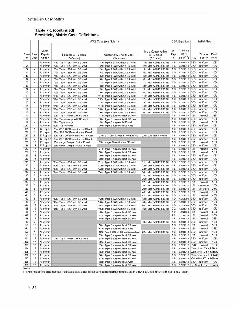
Sensitivity Case Matrix

7-24

Table 7-1 (continued) Sensitivity Matrix Case Definitions

Case#

BaseCase

WeldRepairCase?

K-Exp.

n

C75th,650°F

(in/h;psi-in0.5) 2c/a

ShapeFactor

Depth(%tw)

1 - Axisymm *1a: Type 1 S&R with SS weld *1b: Type 1 S&R without SS weld 1c: Mod ASME 3/30 Fit 1.6 8.515E-12 360° uniform 10%2 - Axisymm *2a: Type 1 S&R with SS weld *2b: Type 1 S&R without SS weld 2c: Mod ASME 3/30 Fit 1.6 8.515E-12 360° uniform 10%3 - Axisymm *3a: Type 1 S&R with SS weld *3b: Type 1 S&R without SS weld 3c: Mod ASME 3/30 Fit 1.6 8.515E-12 360° uniform 10%4 - Axisymm *4a: Type 1 S&R with SS weld *4b: Type 1 S&R without SS weld 4c: Mod ASME 3/30 Fit 1.6 8.515E-12 360° uniform 10%5 - Axisymm *5a: Type 1 S&R with SS weld *5b: Type 1 S&R without SS weld 5c: Mod ASME 3/30 Fit 1.6 8.515E-12 360° uniform 10%6 - Axisymm *6a: Type 1 S&R with SS weld *6b: Type 1 S&R without SS weld 6c: Mod ASME 3/30 Fit 1.6 8.515E-12 360° uniform 10%7 - Axisymm *7a: Type 1 S&R with SS weld *7b: Type 1 S&R without SS weld 7c: Mod ASME 3/30 Fit 1.6 8.515E-12 360° uniform 10%8 - Axisymm *8a: Type 1 S&R with SS weld *8b: Type 1 S&R without SS weld 8c: Mod ASME 3/30 Fit 1.6 8.515E-12 360° uniform 10%9 - Axisymm *9a: Type 1 S&R with SS weld *9b: Type 1 S&R without SS weld 9c: Mod ASME 3/30 Fit 1.6 8.515E-12 360° uniform 10%10 - Axisymm *10a: Type 1 S&R with SS weld *10b: Type 1 S&R without SS weld 10c: Mod ASME 3/30 Fit 1.6 8.515E-12 360° uniform 10%11 - Axisymm *11a: Type 1 S&R with SS weld *11b: Type 1 S&R without SS weld 11c: Mod ASME 3/30 Fit 1.6 8.515E-12 360° uniform 10%12 - Axisymm *12a: Type 1 S&R with SS weld *12b: Type 1 S&R without SS weld 12c: Mod ASME 3/30 Fit 1.6 8.515E-12 360° uniform 10%13 - Axisymm *13a: Type 1 S&R with SS weld *13b: Type 1 S&R without SS weld 13c: Mod ASME 3/30 Fit 1.6 8.515E-12 360° uniform 10%14 - Axisymm *14a: Type 1 S&R with SS weld *14b: Type 1 S&R without SS weld 14c: Mod ASME 3/30 Fit 1.6 8.515E-12 360° uniform 10%15 - Axisymm *15a: Type 1 S&R with SS weld *15b: Type 1 S&R without SS weld 15c: Mod ASME 3/30 Fit 1.6 8.515E-12 360° uniform 10%16 - Axisymm *16a: Type 1 S&R with SS weld *16b: Type 1 S&R without SS weld 16c: Mod ASME 3/30 Fit 1.6 8.515E-12 360° uniform 10%17 - Axisymm 17a: Type 8 surge with SS weld 17b: Type 8 surge without SS weld 1.6 8.515E-12 21 natural 26%18 - Axisymm 18a: Type 8 surge with SS weld 18b: Type 8 surge without SS weld 1.6 8.515E-12 360° uniform 10%19 - Axisymm *19a: Type 9 surge 19b: Type 8 surge with SS weld 1.6 8.515E-12 21 natural 26%20 - Axisymm *20a: Type 9 surge 20b: Type 8 surge with SS weld 1.6 8.515E-12 360° uniform 10%21 1 ID Repair 21a: S&R 20° ID repair / wo SS weld 1.6 8.515E-12 360° uniform 10%22 3 ID Repair 22a: S&R 20° ID repair / wo SS weld 1.6 8.515E-12 360° uniform 10%23 6 ID Repair 23a: S&R 20° ID repair / wo SS weld 23b: S&R 20° ID repair / mod ASME 23c: 23a with 3 repairs 1.6 8.515E-12 360° uniform 10%24 7 ID Repair 24a: S&R 20° ID repair / wo SS weld 1.6 8.515E-12 360° uniform 10%25 17 ID Repair 25a: surge ID repair / with SS weld 25b: surge ID repair / w/o SS weld 1.6 8.515E-12 21 natural 26%26 18 ID Repair 26a: surge ID repair / with SS weld 1.6 8.515E-12 360° uniform 10%27 17 Axisymm 27b: Type 8 surge without SS weld 1.6 8.515E-12 21 natural 26%28 17 Axisymm 28b: Type 8 surge without SS weld 1.6 8.515E-12 21 natural 26%29 18 Axisymm 29b: Type 8 surge without SS weld 1.6 8.515E-12 360° uniform 10%30 18 Axisymm 30b: Type 8 surge without SS weld 1.6 8.515E-12 360° uniform 10%31 1 Axisymm *31a: Type 1 S&R with SS weld *31b: Type 1 S&R without SS weld 31c: Mod ASME 3/30 Fit 1.6 8.515E-12 360° uniform 10%32 1 Axisymm *32a: Type 1 S&R with SS weld *32b: Type 1 S&R without SS weld 32c: Mod ASME 3/30 Fit 1.6 8.515E-12 360° uniform 10%33 4 Axisymm *33a: Type 1 S&R with SS weld *33b: Type 1 S&R without SS weld 33c: Mod ASME 3/30 Fit 1.6 8.515E-12 360° uniform 10%34 4 Axisymm *34a: Type 1 S&R with SS weld *34b: Type 1 S&R without SS weld 34c: Mod ASME 3/30 Fit 1.6 8.515E-12 360° uniform 10%35 6 Axisymm 35c: Mod ASME 3/30 Fit 1.6 8.515E-12 360° uniform 10%36 6 Axisymm 36c: Mod ASME 3/30 Fit 1.6 8.515E-12 360° uniform 10%37 6 Axisymm 37c: Mod ASME 3/30 Fit 1.6 8.515E-12 21 natural 26%38 6 Axisymm 38c: Mod ASME 3/30 Fit 1.6 8.515E-12 21 semi-ellipse 26%39 6 Axisymm 39c: Mod ASME 3/30 Fit 1.6 8.515E-12 21 constant 26%40 6 Axisymm 40c: Mod ASME 3/30 Fit 1.6 8.515E-12 21 natural 15%41 6 Axisymm 41c: Mod ASME 3/30 Fit 1.6 8.515E-12 21 natural 40%42 6 Axisymm *42a: Type 1 S&R with SS weld *42b: Type 1 S&R without SS weld 42c: Mod ASME 3/30 Fit 1.0 4.313E-09 360° uniform 10%43 6 Axisymm *43a: Type 1 S&R with SS weld *43b: Type 1 S&R without SS weld 43c: Mod ASME 3/30 Fit 2.2 1.530E-14 360° uniform 10%44 12 Axisymm *44a: Type 1 S&R with SS weld *44b: Type 1 S&R without SS weld 44c: Mod ASME 3/30 Fit 1.0 4.313E-09 360° uniform 10%45 12 Axisymm *45a: Type 1 S&R with SS weld *45b: Type 1 S&R without SS weld 45c: Mod ASME 3/30 Fit 2.2 1.530E-14 360° uniform 10%46 17 Axisymm 46b: Type 8 surge without SS weld 1.0 4.313E-09 21 natural 26%47 17 Axisymm 47b: Type 8 surge without SS weld 2.2 1.530E-14 21 natural 26%48 17 Axisymm 48b: Type 8 surge without SS weld 1.6 8.515E-12 21 natural 26%49 6 Axisymm 49c: Mod ASME 3/30 Fit 1.6 8.515E-12 360° uniform 10%50 17 Axisymm 50b: Type 8 surge without SS weld 1.6 8.515E-12 21 natural 26%51 19 Axisymm 51b: Type 8 surge with SS weld 1.6 8.515E-12 21 natural 26%52 1 Axisymm 52d: Type 1 S&R w/o SS weld (Interpolated) 52c: Mod ASME 3/30 Fit 1.6 8.515E-12 360° uniform 10%53 17 Axisymm 53b: Type 8 surge without SS weld 1.6 8.515E-12 21 natural 26%S1 17 Axisymm S1a: Type 8 surge with SS weld S1b: Type 8 surge without SS weld 1.6 8.515E-12 360° uniform 10%S2 17 Axisymm S2b: Type 8 surge without SS weld 1.6 8.515E-12 360° uniform 10%S3 17 Axisymm S3b: Type 8 surge without SS weld 1.6 8.515E-12 5.6 natural 10%S4 17 Axisymm S4b: Type 8 surge without SS weld 1.6 8.515E-12S5 17 Axisymm S5b: Type 8 surge without SS weld 1.6 8.515E-12S6 17 Axisymm S6b: Type 8 surge without SS weld 1.6 8.515E-12S7 17 Axisymm S7b: Type 8 surge without SS weld 1.6 8.515E-12S8 19 Axisymm S8b: Type 8 surge with SS weld 1.6 8.515E-12 360° uniform 10%S9 17 Axisymm S9b: Type 8 surge without SS weld 1.6 8.515E-12

Notes(1) Asterisk before case number indicates stable crack arrest verified using axisymmetric crack growth solution for uniform depth 360° crack.

2 Case 17b 21:1 flaws

Combine 17b + 95%tw

Combine 17b + S3b #1Combine 17b + S3b #2Combine 17b + S3b #3

Initial FlawCGR EquationWRS Case (see Note 1)

Conservative WRS Case("b" case)

More ConservativeWRS Case("c" case)

Nominal WRS Case("a" case)

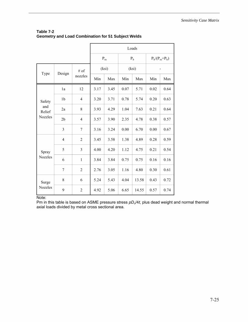
Sensitivity Case Matrix

7-25

Table 7-2 Geometry and Load Combination for 51 Subject Welds

Note: Pm in this table is based on ASME pressure stress pDo/4t, plus dead weight and normal thermal axial loads divided by metal cross sectional area.

Min Max Min Max Min Max

1a 12 3.17 3.45 0.07 5.71 0.02 0.64

1b 4 3.20 3.71 0.78 5.74 0.20 0.63

2a 8 3.93 4.29 1.04 7.63 0.21 0.64

2b 4 3.57 3.90 2.35 4.78 0.38 0.57

3 7 3.16 3.24 0.00 6.70 0.00 0.67

4 2 3.45 3.58 1.38 4.89 0.28 0.59

5 3 4.00 4.20 1.12 4.75 0.21 0.54

6 1 3.84 3.84 0.75 0.75 0.16 0.16

7 2 2.76 3.05 1.16 4.80 0.30 0.61

8 6 5.24 5.43 4.04 13.58 0.43 0.72

9 2 4.92 5.06 6.65 14.55 0.57 0.74

Loads

Pm

Surge Nozzles

(ksi)

Spray Nozzles

Safety and

Relief Nozzles

DesignType-(ksi)

Pb/(Pm+Pb)Pb

# of nozzles

Sensitivity Case Matrix

7-26

Table 7-3 Summary Statistics for Wolf Creek Pressurizer Surge Nozzle DM Weld Indications Reported in October 2006

(%tw

)(in

)

Star

ton

OD

(in)

Sto

pon

OD

(in)

on OD

(in)

on ID (in)

Sta

rt(%

Circ

)S

top

(%C

irc)

(%C

irc)

(deg

)

Tota

l ID

Leng

ths

(in)

Tota

l % o

fEn

velo

peLe

ngth

Ind#

1% o

fE

nvel

ope

Leng

th(in

2 )(%

wal

l)

Tota

lAr

eas

(%w

all)

Tota

l % o

fE

nvel

ope

Are

a

Ind#

1% o

fE

nvel

ope

Are

aIn

dica

tion

#110

%0.

145

43.0

44.0

1.0

0.81

5.6

91.5

%93

.6%

2.1%

7.7

0.12

0.19

%In

dica

tion

#225

%0.

363

28.7

531

.52.

752.

226.

161

.2%

67.0

%5.

9%21

.10.

831.

3%In

dica

tion

#331

%0.

450

20.5

25.5

5.0

4.03

9.0

43.6

%54

.3%

10.6

%38

.31.

883.

1%

Env

elop

e 2&

331

%0.

450

20.5

31.5

11.0

8.87

19.7

43.6

%67

.0%

23.4

%84

.36.

2570

.5%

4.13

6.7%

4.4%

65.5

%En

velo

pe 1

,2&

331

%0.

450

20.5

44.0

23.5

18.9

442

.143

.6%

93.6

%50

.0%

180.

07.

0537

.2%

4.3%

8.83

14.4

%4.

6%32

.0%

1.3%

Wel

d O

D C

ircum

fere

nce

(in)

47.0

Not

es:

OD

(in)

14.9

6(1

) Con

stan

t dep

th s

hape

ass

umed

for f

law

are

a ca

lcul

atio

ns.

Wel

d Th

ickn

ess,

t (in

)1.

45ID

(in)

12.0

6ID

/OD

0.80

6C

ross

Sec

tiona

l Are

a (in

2 )61

.54

Ass

umed

Flaw

Max

. Dep

thLe

ngth

Circ

.P

ositi

onIn

divi

dual

Flaw

Len

gths

Flaw

Are

a(N

ote

1)In

divi

dual

Flaw

Are

asLe

ngth

-to

-Dep

thAs

pect

Rat

io

Circ

.Po

sitio

nC

irc.

Exte

nt

Sensitivity Case Matrix

7-27

Table 7-4 Sensitivity Matrix Case Surface Crack Results

NozzleType

GeometryConfiguration

Ri

(in)t

(in)

Timeto TW(yrs)

FractionXsectionCracked

CrackFace

F (kips)

Max totFaxial(kips)

Max PmBased onCF (ksi)

StabilityMarginFactor

Support.Pm(ksi)

Support.Pb (thick)

(ksi)1 c S&R Config 1a 2.585 1.290 17.4 0.400 23.40 72.74 2.78 3.10 8.6 17.72 c S&R Config 1a 2.585 1.290 21.3 0.395 23.12 72.45 2.77 3.33 9.2 17.63 c S&R Config 1a 2.585 1.290 26.3 0.383 22.43 71.77 2.74 3.67 10.1 17.94 c S&R Config 1b 2.595 1.405 18.0 0.400 26.04 88.68 3.05 2.95 9.0 16.95 c S&R Config 1b 2.595 1.405 25.7 0.381 24.79 87.44 3.00 3.51 10.6 17.26 c S&R Config 2a/2b 2.810 1.065 3.4 0.435 21.74 82.16 3.67 2.04 7.5 15.67 c S&R Config 2a/2b 2.810 1.065 10.5 0.440 22.01 82.43 3.69 2.63 9.7 12.68 c S&R Config 3 2.595 1.405 13.4 0.399 25.94 74.96 2.58 2.87 7.4 19.29 c S&R Config 3 2.595 1.405 32.2 0.364 23.69 72.71 2.50 4.12 10.3 20.110 c spray Config 4 2.005 0.900 21.2 0.389 12.06 39.94 2.88 3.57 10.3 17.411 c spray Config 4 2.005 0.900 25.3 0.378 11.71 39.59 2.85 3.95 11.3 17.812 c spray Config 5 2.125 0.780 10.5 0.436 12.01 44.18 3.58 2.76 9.9 13.113 c spray Config 5 2.125 0.780 13.6 0.427 11.76 43.94 3.56 3.05 10.9 12.614 c spray Config 6 2.850 1.15015 c spray Config 7 1.550 1.04516 c spray Config 7 1.550 1.04517 a surge Config 8 5.920 1.58017 b surge Config 8 5.920 1.580 1.2 0.240 35.80 289.91 4.35 1.73 7.5 23.418 a surge Config 8 5.920 1.58018 b surge Config 8 5.920 1.580 11.5 0.499 74.22 328.34 4.93 2.05 10.1 10.019 b surge Config 9 5.060 1.47020 b surge Config 9 5.060 1.47021 a S&R Config 1a 2.585 1.290 0.6 0.212 12.41 61.75 2.36 5.08 12.0 29.022 a S&R Config 1a 2.585 1.290 0.6 0.213 12.44 61.78 2.36 5.58 13.2 27.223 a S&R Config 2a/2b 2.810 1.065 0.4 0.208 10.40 70.82 3.17 3.79 12.0 28.923 b S&R Config 2a/2b 2.810 1.065 0.4 0.275 13.74 74.16 3.32 3.37 11.2 25.723 c S&R Config 2a/2b 2.810 1.065 0.5 0.298 14.91 75.33 3.37 3.55 12.0 27.124 a S&R Config 2a/2b 2.810 1.065 0.5 0.210 10.49 70.91 3.17 6.09 19.3 29.125 a surge Config 8 5.920 1.580 0.8 0.173 25.73 279.84 4.20 2.13 9.0 28.925 b surge Config 8 5.920 1.580 0.5 0.183 27.21 281.33 4.22 2.07 8.7 28.026 a surge Config 8 5.920 1.580 2.2 0.359 53.51 307.62 4.62 2.88 13.3 14.127 b surge bounding 5.920 1.580 1.3 0.243 36.20 290.32 4.36 1.76 7.7 22.928 b surge bounding 5.920 1.580 2.0 0.271 40.31 294.42 4.42 1.92 8.5 19.229 b surge bounding 5.920 1.580 7.1 0.527 78.39 332.50 4.99 1.47 7.3 10.330 b surge bounding 5.920 1.58031 c S&R as-built 1 2.585 1.419 35.2 0.369 24.22 73.55 2.50 3.97 10.0 20.032 c S&R as-built 2 2.585 1.161 7.5 0.417 21.50 70.83 3.07 2.58 7.9 16.933 c S&R bounding S&R 2.595 1.405 19.8 0.388 25.22 87.87 3.02 3.10 9.4 17.834 c S&R bounding S&R 2.595 1.405 14.6 0.407 26.50 89.15 3.06 2.86 8.8 16.435 c S&R bounding S&R 2.810 1.065 2.9 0.447 22.33 82.75 3.70 1.93 7.2 14.836 c S&R bounding S&R 2.810 1.065 3.6 0.434 21.69 82.11 3.67 2.05 7.5 15.637 c S&R bounding S&R 2.810 1.065 3.4 0.332 16.59 77.01 3.44 2.32 8.0 17.738 c S&R bounding S&R 2.810 1.065 3.4 0.331 16.56 76.98 3.44 2.32 8.0 17.739 c S&R bounding S&R 2.810 1.065 3.4 0.340 16.99 77.41 3.46 2.29 7.9 17.440 c S&R bounding S&R 2.810 1.065 3.9 0.308 15.38 75.80 3.39 2.44 8.3 18.641 c S&R bounding S&R 2.810 1.065 2.6 0.357 17.83 78.25 3.50 2.22 7.8 17.042 c S&R bounding S&R 2.810 1.065 1.8 0.476 23.79 84.21 3.77 1.68 6.3 12.843 c S&R bounding S&R 2.810 1.065 7.6 0.408 20.41 80.83 3.61 2.27 8.2 17.344 c spray bounding spray 2.125 0.780 2.9 0.470 12.94 45.11 3.66 2.34 8.6 11.145 c spray bounding spray 2.125 0.780 48.1 0.417 11.50 43.67 3.54 2.97 10.5 14.146 b surge bounding surge 5.920 1.580 1.1 0.236 35.14 289.26 4.34 1.74 7.5 23.647 b surge bounding surge 5.920 1.580 1.5 0.247 36.77 290.88 4.37 1.71 7.5 23.248 b surge bounding 5.920 1.580 1.2 0.240 35.80 289.91 4.35 1.73 7.5 23.449 c S&R bounding 2.810 1.065 3.4 0.435 21.74 77.35 3.46 3.96 13.7 3.750 b surge bounding 5.920 1.580 1.2 0.240 35.80 287.63 4.32 4.37 18.9 3.551 b surge bounding 5.060 1.47052 c S&R example S&R 2.585 1.318 11.6 0.422 25.34 74.68 2.78 2.88 8.0 16.052 d S&R example S&R 2.585 1.31853 b surge example surge 5.920 1.580 1.1 0.244 36.33 290.45 4.36 1.70 7.4 23.1S1 a surge Config 8 5.920 1.580S1 b surge Config 8 5.920 1.580 1.2 0.489 72.76 326.88 4.91 1.08 5.3 14.6S2 b surge Config 8 5.920 1.580 3.4 0.518 77.12 331.23 4.97 1.37 6.8 11.5S3 b surge Config 8 5.920 1.580 2.2 0.179 26.63 280.74 4.21 2.10 8.8 28.4S4 b surge Config 8 5.920 1.580S5 b surge Config 8 5.920 1.580S6 b surge Config 8 5.920 1.580S7 b surge Config 8 5.920 1.580S8 b surge Config 9 5.060 1.470S9 b surge Config 8 5.920 1.580

ArrestN/A

Arrest

N/A

N/AN/AN/A

Arrest

ArrestArrest

Arrest

Arrest

Arrest

Surface Crack Stability Results (Press + DW + NT loads and Z-factor for Critical Size)

Arrest

Geometry Case

Arrest

Case#

Arrest

Arrest

WR

S Su

bcas

e

Sensitivity Case Matrix

7-28

Table 7-5 Sensitivity Matrix Case Through-Wall Crack Results at 1 gpm or Initial Leak Rate if Higher

Case and Step

FractionXsectionCracked

CrackFaceForce (kips)

Max totFaxial(kips)

Max PmBased on CF (ksi)

Support.Pm(ksi)

Support.Pb (thick)

(ksi)

StabilityMarginFactor

Time since TW

(hrs)

Time since TW

(days)

Leak Rate(gpm @

70°F)01cS13 0.466 27.27 76.61 2.93 6.55 12.78 2.24 2726 114 1.0402cS14 0.470 27.48 76.82 2.93 6.79 12.25 2.31 3416 142 1.0503cS15 0.472 27.59 76.93 2.94 7.04 11.70 2.40 4358 182 1.0704cS12 0.462 30.06 92.71 3.18 6.95 12.52 2.18 2567 107 1.0005cS14 0.466 30.30 92.95 3.19 7.50 11.47 2.35 4328 180 1.0006cS13 0.471 23.53 83.96 3.75 6.37 12.95 1.70 752 31 1.0407cS21 0.491 24.53 84.95 3.80 7.64 9.62 2.01 1682 70 1.0208cS12 0.459 29.88 78.91 2.71 5.79 14.32 2.14 2268 94 1.0909cS16 0.470 30.56 79.58 2.73 6.84 12.21 2.50 5489 229 1.0810cS20 0.497 15.42 43.30 3.12 6.46 10.13 2.07 4690 195 1.0111cS22 0.506 15.69 43.57 3.14 6.54 9.38 2.08 6251 260 1.0412cS17 0.507 13.96 46.13 3.74 6.95 8.82 1.86 2639 110 1.0313cS18 0.512 14.10 46.28 3.75 7.29 8.03 1.94 3120 130 1.0314cSna15cSna16cSna17aSna17bS00 0.243 36.18 290.30 4.36 7.44 23.17 1.71 0 0 2.5518aSna18bS00 0.523 77.93 332.04 4.98 8.94 8.75 1.79 0 0 2.7119bSna20bSna21aS16 0.255 14.95 64.28 2.46 10.86 25.26 4.42 1762 73 1.0222aS17 0.260 15.23 64.57 2.47 11.78 23.31 4.78 1894 79 1.0623aS13 0.248 12.38 72.80 3.26 10.92 25.59 3.36 1194 50 1.0123bS02 0.311 15.55 75.98 3.40 10.13 22.75 2.98 194 8 1.0623cS16 0.369 18.44 78.87 3.53 10.53 22.76 2.99 1799 75 1.0024aS15 0.255 12.75 73.17 3.27 13.86 20.25 4.24 1607 67 1.0325aS00 0.175 25.99 280.10 4.20 8.92 28.78 2.12 0 0 5.2825bS00 0.185 27.47 281.58 4.23 8.68 27.88 2.05 0 0 6.0326aS00 0.364 54.17 308.29 4.63 13.12 13.84 2.83 0 0 1.1827bS00 0.246 36.58 290.69 4.36 7.61 22.68 1.74 0 0 2.5028bS00 0.355 52.84 306.96 4.61 7.71 16.74 1.67 0 0 2.4329bS00 0.537 79.95 334.07 5.02 6.91 9.65 1.38 0 0 4.0530bSna31cS16 0.471 30.90 80.23 2.73 6.73 12.37 2.46 5656 236 1.0632cS11 0.471 24.32 73.66 3.19 6.26 12.86 1.96 1847 77 1.0233cS13 0.460 29.94 92.59 3.18 6.98 12.60 2.20 3374 141 1.0034cS12 0.468 30.45 93.09 3.20 6.77 12.16 2.12 2346 98 1.0635cS06 0.480 23.98 84.40 3.77 6.13 12.38 1.62 617 26 1.1036cS08 0.471 23.56 83.98 3.75 6.35 12.89 1.69 857 36 1.0537cS19 0.419 20.96 81.38 3.64 6.67 13.98 1.83 1024 43 1.0138cS19 0.420 21.02 81.44 3.64 6.67 13.98 1.83 1035 43 1.0139cS19 0.424 21.22 81.64 3.65 6.62 13.82 1.81 993 41 1.0340cS22 0.410 20.47 80.89 3.62 6.82 14.39 1.89 1151 48 1.0141cS18 0.434 21.68 82.10 3.67 6.51 13.53 1.77 957 40 1.0342cS00 0.487 24.36 84.79 3.79 5.96 12.00 1.57 0 0 1.0743cS09 0.452 22.58 83.00 3.71 6.82 14.01 1.84 1035 43 1.0044cS09 0.528 14.55 46.72 3.79 6.41 8.04 1.69 1228 51 1.0145cS19 0.501 13.81 45.98 3.73 7.14 9.10 1.91 3284 137 1.0646bS00 0.240 35.69 289.80 4.35 7.45 23.25 1.71 0 0 4.6347bS00 0.248 36.95 291.07 4.37 7.42 23.03 1.70 0 0 1.3848bS00 0.243 21.53 275.65 4.14 7.18 23.54 1.73 0 0 2.4249cS30 0.502 25.10 80.71 3.61 10.30 2.68 2.85 4004 167 1.0150bS00 0.243 36.19 288.03 4.32 18.70 3.42 4.33 0 0 1.0751bSna52cS10 0.470 28.22 77.55 2.89 6.51 12.52 2.26 1658 69 1.0052dSna53bS00 0.246 36.68 290.80 4.37 7.36 22.88 1.69 0 0 2.39S1aSnaS1bS00 0.496 73.89 328.00 4.92 5.08 14.01 1.03 0 0 7.39S2bS00 0.529 78.83 332.95 5.00 6.38 10.72 1.28 0 0 4.87S3bS00 0.188 28.04 282.15 4.24 8.61 27.58 2.03 0 0 2.43S4bSna* 0.400 59.53 313.64 4.71 6.75 19.44 1.43 167 7 2.55S5bSna* 0.400 59.53 313.64 4.71 6.95 20.02 1.48 167 7 2.55S6bSna* 0.400 59.53 313.64 4.71 6.10 17.57 1.29 167 7 2.55S7bSna* 0.453 67.50 321.61 4.83 6.95 19.52 1.44 167 7 2.55S8bSnaS9bS00 0.322 47.95 302.06 4.53 7.24 21.65 1.60 0 0 2.55

*Stability results after 7 days of detectable leakage for these multiple flaw cases only (S4b through S7b)

Arrest

Arrest

Arrest

Arrest

Arrest

Arrest

ArrestArrest

Arrest

Arrest

ArrestArrest

Sensitivity Case Matrix

7-29

Table 7-6 Sensitivity Matrix Case Through-Wall Crack Results at Load Margin Factor of 1.2

Case and Step

FractionXsectionCracked

CrackFaceForce (kips)

Max totFaxial(kips)

Max PmBasedon CF (ksi)

Support.Pm(ksi)

Support.Pb (thick)

(ksi)

StabilityMarginFactor

Time since TW

(hrs)

Time sinceTW

(days)

Time since 1

gpm (hrs)

Time since 1

gpm (days)

Leak Rate

(gpm @ 70°F)

01cS36 0.568 33.21 82.55 3.15 3.80 6.89 1.21 5350 223 2623 109 5.8102cS37 0.574 33.61 82.95 3.17 3.85 6.43 1.21 6255 261 2839 118 5.8903cS38 0.580 33.93 83.26 3.18 3.88 5.95 1.22 7357 307 2998 125 6.2204cS34 0.558 36.29 98.94 3.40 4.19 7.07 1.23 5252 219 2685 112 5.2205cS37 0.574 37.36 100.01 3.44 4.15 5.90 1.21 7615 317 3288 137 5.8106cS41 0.529 26.45 86.87 3.88 4.70 9.23 1.21 1741 73 989 41 4.0407cS62 0.573 28.64 89.06 3.98 4.79 5.75 1.20 3389 141 1706 71 5.4408cS34 0.553 36.00 85.03 2.92 3.58 8.21 1.23 4643 193 2375 99 5.5809cS41 0.586 38.10 87.13 2.99 3.63 5.93 1.21 8942 373 3453 144 6.5610cS38 0.582 18.05 45.92 3.31 3.98 5.89 1.20 6450 269 1760 73 3.8011cS39 0.587 18.21 46.09 3.32 4.09 5.54 1.23 7996 333 1745 73 3.7012cS33 0.575 15.83 48.00 3.89 4.66 5.69 1.20 3801 158 1163 48 3.5413cS34 0.582 16.04 48.21 3.91 4.83 5.10 1.23 4414 184 1295 54 3.4914cSna15cSna16cSna17aSna17bS73 0.331 49.30 303.42 4.55 5.45 16.24 1.20 829 35 829 35 69.2818aSna18bS21 0.591 88.03 342.15 5.14 6.15 5.84 1.20 1022 43 1022 43 15.7919bS3220bSna21aS20 0.270 15.78 65.12 2.49 10.47 24.04 4.21 2272 95 509 >>21 1.2822aS20 0.271 15.84 65.18 2.49 11.46 22.47 4.60 2295 96 400 >>17 1.2523aS21 0.278 13.91 74.34 3.32 10.05 23.06 3.02 2085 87 891 >>37 1.6723bS33 0.517 25.84 86.26 3.86 4.64 9.18 1.20 4354 181 4160 173 6.4423cS20 0.387 19.34 79.76 3.57 10.08 21.57 2.83 2296 96 497 >>21 1.2724aS19 0.270 13.48 73.90 3.30 13.31 19.26 4.03 2115 88 508 >>21 1.3125aS75 0.330 49.10 303.22 4.55 5.49 16.36 1.21 1868 78 1868 78 98.5125bS79 0.329 49.04 303.15 4.55 5.49 16.37 1.21 1642 68 1642 68 91.8626aS09 0.383 57.09 311.21 4.67 12.24 12.79 2.62 958 40 958 >>40 5.4027bS68 0.337 50.12 304.24 4.57 5.50 15.64 1.20 919 38 919 38 70.4328bS30 0.424 63.08 317.20 4.76 5.71 12.00 1.20 655 27 655 27 28.7529bS08 0.560 83.38 337.50 5.07 6.07 8.38 1.20 267 11 267 11 8.4930bSna31cS40 0.588 38.59 87.92 2.99 3.58 6.00 1.20 9163 382 3507 146 6.4332cS31 0.552 28.50 77.84 3.37 4.07 7.91 1.21 3616 151 1769 74 4.8033cS35 0.560 36.46 99.10 3.40 4.11 6.94 1.21 6338 264 2964 123 5.2734cS34 0.561 36.51 99.16 3.41 4.11 6.93 1.21 4709 196 2363 98 5.5235cS18 0.528 26.38 86.80 3.88 4.76 9.35 1.23 1393 58 776 32 3.6736cS24 0.529 26.43 86.86 3.88 4.70 9.24 1.21 1870 78 1013 42 3.9937cS57 0.503 25.16 85.58 3.83 4.58 9.14 1.20 2193 91 1170 49 4.9738cS56 0.504 25.21 85.63 3.83 4.58 9.12 1.20 2210 92 1175 49 4.9839cS55 0.504 25.22 85.64 3.83 4.60 9.16 1.20 2117 88 1124 47 4.8740cS63 0.501 25.05 85.47 3.82 4.59 9.16 1.20 2424 101 1273 53 5.1841cS52 0.508 25.39 85.81 3.84 4.60 9.14 1.20 2009 84 1052 44 4.7042cS15 0.534 26.71 87.13 3.90 4.66 9.12 1.20 927 39 927 39 2.9743cS30 0.525 26.26 86.68 3.88 4.68 9.21 1.21 2171 90 1135 47 4.8444cS18 0.581 16.01 48.18 3.91 4.80 5.84 1.23 2125 89 898 37 2.6445cS37 0.573 15.78 47.95 3.89 4.69 5.73 1.21 4397 183 1113 46 3.8646bS44 0.330 49.07 303.18 4.55 5.48 16.33 1.20 1755 73 1755 73 73.5847bS85 0.331 49.25 303.37 4.55 5.48 16.32 1.20 534 22 534 22 63.3448bS76 0.335 29.71 283.82 4.26 5.12 16.32 1.20 941 39 941 39 70.0549cS86 0.628 31.37 86.98 3.89 4.67 1.13 1.20 7474 311 3470 145 8.57

50bS150 0.492 73.20 325.04 4.88 6.14 0.99 1.26 7034 293 7034 293 191.4351bSna52cS35 0.567 34.07 83.40 3.10 3.84 6.87 1.24 3916 163 2257 94 6.6152dSna53bS103 0.331 49.29 303.41 4.55 5.46 16.26 1.20 1164 49 1164 49 42.35S1aSnaS1bSnaS2bS01 0.537 79.90 334.01 5.01 6.14 10.28 1.22 82 3 (Note 1) 82 3 (Note 1) 6.00S3bS93 0.330 49.16 303.27 4.55 5.47 16.30 1.20 1772 74 1772 74 87.49S4bSnaS5bSnaS6bSnaS7bSnaS8bSnaS9bSna 0.415 61.74 315.86 4.74 5.17 14.81 1.09 829 35 (Note 2) 829 35 (Note 2) 69.28

Note 1: Case S2b showed 4 days from initial leakage (at 4.9 gpm) until load margin factor of 1.20 based on interpolation.Note 2: Case S9b showed 29 days from initial leakage (at 2.6 gpm) until load margin factor of 1.20 based on interpolation.

Arrest

Arrest

Not Applicable

Not Applicable -- @ TW Load Factor = 1.08 (1.03 at first leakage) / 2 days from TW to load factor of 1.0Arrest

Arrest

Arrest

Arrest

Arrest

Arrest

Arrest

ArrestArrestArrest

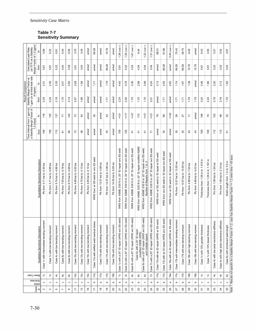
Sensitivity Case Matrix

7-30

Table 7-7 Sensitivity Summary

from

tofro

mto

from

to

2c

1cC

ase

1c w

ith in

term

edia

te b

endi

ng m

omen

tP

b fro

m 5

.71

ksi t

o 5

.30

ksi

109

118

2.24

2.31

5.81

5.89

3c

1cC

ase

1c w

ith lo

w b

endi

ng m

omen

tP

b fro

m 5

.71

ksi t

o 4

.88

ksi

109

125

2.24

2.40

5.81

6.22

5c

4cC

ase

4c w

ith lo

w b

endi

ng m

omen

tP

b fro

m 5

.74

ksi t

o 4

.88

ksi

112

137

2.18

2.35

5.22

5.81

7c

6cC

ase

6c w

ith lo

w b

endi

ng m

omen

tP

b fro

m 7

.63

ksi t

o 4

.78

ksi

4171

1.70

2.01

4.04

5.44

9c

8cC

ase

8c w

ith lo

w b

endi

ng m

omen

tP

b fro

m 6

.70

ksi t

o 4

.88

ksi

9914

42.

142.

505.

586.

56

11c

10c

Cas

e 10

c w

ith lo

w b

endi

ng m

omen

tP

b fro

m 4

.89

ksi t

o 4

.50

ksi

7373

2.07

2.08

3.81

3.70

13c

12c

Cas

e 12

c w

ith lo

w b

endi

ng m

omen

tP

b fro

m 4

.75

ksi t

o 4

.13

ksi

4854

1.86

1.94

3.54

3.49

16c

15c

Cas

e 15

c w

ith lo

w b

endi

ng m

omen

tP

b fro

m 4

.65

ksi t

o 4

.13

ksi

arre

star

rest

arre

star

rest

arre

star

rest

17b

17a

Cas

e 17

a w

ith s

hifte

d w

eld

resi

dual

stre

ssW

RS

from

w/ S

S w

eld

to w

/o S

S w

eld

arre

st35

arre

st1.

71ar

rest

69.2

8

18a

17a

Cas

e 17

a w

ith lo

w b

endi

ng m

omen

tP

b fro

m 1

3.57

ksi

to 4

.88

ksi

arre

star

rest

arre

star

rest

arre

star

rest

18b

17b

Cas

e 17

b w

ith lo

w b

endi

ng m

omen

tP

b fro

m 1

3.57

ksi

to 4

.88

ksi

3543

1.71

1.79

69.2

815

.79

20b

19b

Cas

e 19

b w

ith lo

w b

endi

ng m

omen

tP

b fro

m 1

4.55

ksi

to 6

.65

ksi

arre

star

rest

arre

star

rest

arre

star

rest

21a

1cC

ase

1c w

ith a

20°

ID re

pair

(WR

S w

/o S

S w

eld)

WR

S fr

om A

SM

E 3

/30

fit to

20°

ID re

pair

w/o

SS

wel

d10

9>>

212.

244.

425.

811.

28 (n

ote

1)

22a

3cC

ase

3c w

ith a

20°

ID re

pair

(WR

S w

/o S

S w

eld)

WR

S fr

om A

SM

E 3

/30

fit to

20°

ID re

pair

w/o

SS

wel

d12

5>>

172.

404.

786.

221.

25 (n

ote

1)

23a

6cC

ase

6c w

ith a

20°

ID re

pair

(WR

S w

/o S

S w

eld)

WR

S fr

om A

SM

E 3

/30

fit to

20°

ID re

pair

w/o

SS

wel

d41

>>37

1.70

3.36

4.04

1.67

(not

e 1)

23b

6cC

ase

6c w

ith a

20°

ID re

pair

(mod

ified

AS

ME

WR

S)W

RS

from

AS

ME

3/30

fit t

o 2

0° ID

repa

ir m

odifi

ed A

SME

4117

31.

702.

984.

046.

44

23c

6cC

ase

6c w

ith a

20°

ID re

pair

(WR

S w

/o S

S w

eld)

an

d m

ultip

le re

pairs

WR

S fr

om A

SM

E 3

/30

fit to

20°

ID re

pair

w/o

SS

wel

d;

N

umbe

r of R

epai

rs fr

om 1

to 3

41

>>21

1.70

2.99

4.04

1.22

(not

e 1)

24a

7cC

ase

7c w

ith a

20°

ID re

pair

(WR

S w

/o S

S w

eld)

WR

S fr

om A

SM

E 3

/30

fit to

20°

ID re

pair

w/o

SS

wel

d71

>>21

2.01

4.24

5.44

1.31

(not

e 1)

25a

17a

Cas

e 17

a w

ith a

n ID

repa

ir (W

RS

w/ S

S w

eld)

WR

S fr

om w

/ SS

wel

d to

ID re

pair

w/ S

S w

eld

arre

st78

arre

st2.

12ar

rest

98.5

1

25b

17b

Cas

e 17

b w

ith a

n ID

repa

ir (W

RS

w/o

SS

wel

d)W

RS

from

w/o

SS

wel

d to

ID

repa

ir w

/o S

S w

eld

3568

1.71

2.05

69.2

891

.86

26a

18a

Cas

e 18

a w

ith a

n ID

repa

ir (W

RS

w/ S

S w

eld)

WR

S fr

om w

/ SS

wel

d to

ID re

pair

w/ S

S w

eld

arre

st>>

40ar

rest

2.83

arre

st5.

40 (n

ote

1)

27b

17b

Cas

e 17

b w

ith in

term

edia

te b

endi

ng m

omen

tP

b fro

m 1

3.57

ksi

to 1

3.00

ksi

3538

1.71

1.74

69.2

870

.43

28b

17b

Cas

e 17

b w

ith lo

w b

endi

ng m

omen

tP

b fro

m 1

3.57

ksi

to 1

0.00

ksi

3527

1.71

1.67

69.2

828

.75

29b

18b

Cas

e 18

b w

ith h

igh

bend

ing

mom

ent

Pb

from

4.8

8 ks

i to

7.0

0 ks

i43

111.

791.

3815

.79

8.49

30b

18b

Cas

e 18

b w

ith lo

w b

endi

ng m

omen

tP

b fro

m 4

.88

ksi t

o 4

.03

ksi

43ar

rest

1.79

arre

st15

.79

arre

st

31c

1cC

ase

1c w

ith 1

0% g

reat

er th

ickn

ess

Thic

knes

s fro

m 1

.29

in to

1.4

19 in

109

146

2.24

2.46

5.81

6.43

32c

1cC

ase

1c w

ith 1

0% le

sser

thic

knes

sTh

ickn

ess

from

1.2

9 in

to 1

.161

in10

974

2.24

1.96

5.81

4.80

33c

4cC

ase

4c w

ith lo

w a

xial

mem

bran

e st

iffne

ssP

m fr

om 1

.90

ksi t

o 1

.64

ksi

112

123

2.18

2.20

5.22

5.27

34c

4cC

ase

4c w

ith h

igh

axia

l mem

bran

e st

iffne

ssP

m fr

om 1

.90

ksi t

o 2

.15

ksi

112

982.

182.

125.

225.

52

35c

6cC

ase

6c w

ith s

horte

ned

wel

d le

ngth

Wel

d Le

ngth

from

1 in

to 0

.5 in

4132

1.70

1.62

4.04

3.67

Not

e 1:

Res

ults

not

spe

cific

for a

Sta

bilit

y M

argi

n Fa

ctor

of 1

.2; c

ase

has

Sta

bilit

y M

argi

n Fa

ctor

>>

1.2

whe

n tim

e >

40 d

ays

Base Case

WRS Subcase

Cas

e #

Qua

litat

ive

Sens

itivi

ty D

escr

iptio

nQ

uant

itativ

e S

ensi

tivity

Des

crip

tion

Res

ult C

ompa

rison

Tim

e In

terv

al fr

om 1

gpm

to

a S

tabi

lity

Mar

gin

Fact

or o

f 1.

2 [d

ays]

Cal

cula

ted

Leak

Rat

e

(a

t 70°

F) a

t a S

tabi

lity

Mar

gin

Fact

or o

f 1.2

[gpm

]

Sta

bilit

y M

argi

n Fa

ctor

at

1

gpm

(or a

t ini

tial l

eak

rate

if

high

er)

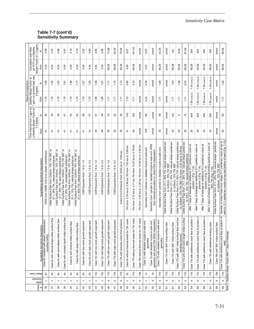
Sensitivity Case Matrix

7-31

Table 7-7 (cont’d) Sensitivity Summary

from

tofro

mto

from

to

36c

6cC

ase

6c m

odel

ed w

ith p

last

ic re

dist

ribut

ion

(mod

ified

WR

S)

WR

S fro

m A

SM

E 3

/30

fit to

pla

stic

redi

strib

utio

n41

421.

701.

694.

043.

99

37c

6cC

ase

6c w

ith n

atur

al s

hape

initi

al s

urfa

ce fl

awIn

itial

Sur

face

Fla

w fr

om U

nifo

rm, 1

0% T

W 3

60°

to

21:1

, 26%

TW

, nat

ural

sha

pe p

artia

l-arc

4149

1.70

1.83

4.04

4.97

38c

6cC

ase

6c w

ith s

emi-e

llipse

initi

al s

urfa

ce fl

awIn

itial

Sur

face

Fla

w fr

om U

nifo

rm, 1

0% T

W 3

60°

to

21:1

, 26%

TW

, sem

i-ellip

se p

artia

l-arc

4149

1.70

1.83

4.04

4.98

39c

6cC

ase

6c w

ith c

onst

ant d

epth

initi

al s

urfa

ce fl

awIn

itial

Sur

face

Fla

w fr

om U

nifo

rm, 1

0% T

W 3

60°

to

21:1

, 26%

TW

, con

stan

t dep

th p

artia

l-arc

4147

1.70

1.81

4.04

4.87

40c

6cC

ase

6c w

ith s

hallo

w in

itial

sur

face

flaw

Initi

al S

urfa

ce F

law

from

Uni

form

, 10%

TW

360

° to

21

:1, 1

5% T

W, n

atur

al s

hape

par

tial-a

rc41

531.

701.

894.

045.

18

41c

6cC

ase

6c w

ith d

eep

initi

al s

urfa

ce fl

awIn

itial

Sur

face

Fla

w fr

om U

nifo

rm, 1

0% T

W 3

60°

to

21:1

, 40%

TW

, nat

ural

sha

pe p

artia

l-arc

4144

1.70

1.77

4.04

4.70

42c

6cC

ase

6c w

ith lo

w c

rack

gro

wth

exp

onen

tC

GR

Exp

onen

t fro

m 1

.6 to

1.0

4139

1.70

1.57

4.04

2.97

43c

6cC

ase

6c w

ith h

igh

crac

k gr

owth

exp

onen

tC

GR

Exp

onen

t fro

m 1

.6 to

2.2

4147

1.70

1.84

4.04

4.84

44c

12c

Cas

e 12

c w

ith lo

w c

rack

gro

wth

exp

onen

tC

GR

Exp

onen

t fro

m 1

.6 to

1.0

4837

1.86

1.69

3.54

2.64

45c

12c

Cas

e 12

c w

ith h

igh

crac

k gr

owth

exp

onen

tC

GR

Exp

onen

t fro

m 1

.6 to

2.2

4846

1.86

1.91

3.54

3.86

46b

17b

Cas

e 17

b w

ith lo

w c

rack

gro

wth

exp

onen

tC

GR

Exp

onen

t fro

m 1

.6 to

1.0

3573

1.71

1.71

69.2

873

.58

47b

17b

Cas

e 17

b w

ith h

igh

crac

k gr

owth

exp

onen

tC

GR

Exp

onen

t fro

m 1

.6 to

2.2

3522

1.71

1.70

69.2

863

.34

48b

17b

Cas

e 17

b w

ith re

duce

d cr

ack

front

pre

ssur

eC

rack

Fro

nt P

ress

ure

from

223

5 ps

i to

133

0 ps

i35

391.

711.

7369

.28

70.0

5

49c

6cC

ase

6c w

ithou

t the

rmal

load

s fo

r TW

cra

ckP

m fr

om 2

.34

ksi t

o 2

.46

ksi;

Pb

from

7.6

3 ks

i to

0.9

4 ks

i41

145

1.70

2.85

4.04

8.57

50b

17b

Cas

e 17

b w

ithou

t the

rmal

load

s fo

r TW

cra

ckP

m fr

om 3

.72

ksi t

o 3

.71

ksi;

Pb

from

13.

57 k

si to

0.7

9 ks

i35

293

1.71

4.33

69.2

819

1.43

51b

19b

Cas

e 19

b w

ithou

t the

rmal

load

s fo

r TW

cra

ckP

m fr

om 3

.45

ksi t

o 3

.36

ksi;

Pb

from

14.

55 k

si to

0.9

0 ks

iar

rest

arre

star

rest

arre

star

rest

arre

st

52c

1cC

ase

1c w

ith d

etai

led

nozz

le-to

-saf

e en

d ge

omet

ryG

eom

etry

from

cyl

inde

r to

deta

iled

nozz

le-to

-saf

e en

d10

994

2.24

2.26

5.81

6.61

52d

1bC

ase

1b w

ith d

etai

led

nozz

le-to

-saf

e en

d ge

omet

ry a

nd d

irect

FE

A W

RS

inte

rpol

atio

nG

eom

etry

from

cyl

inde

r to

deta

iled

nozz

le-to

-saf

e en

d; W

RS

from

the

rmal

sim

ulat

ion

to d

irect

FEA

inte

rpol

atio

nar

rest

arre

star

rest

arre

star

rest

arre

st

53b

17b

Cas

e 17

b w

ith d

etai

led

nozz

le-to

-saf

e en

d ge

omet

ryG

eom

etry

from

cyl

inde

r to

deta

iled

nozz

le-to

-saf

e en

d35

491.

711.

6969

.28

42.3

5

S1

a17

aC

ase

17a

with

360

° in

itial

sur

face

flaw

Initi

al S

urfa

ce F

law

from

21:1

, 26%

TW

, nat

ural

sha

pe p

artia

l-arc

to U

nifo

rm, 1

0% T

W 3

60°

arre

star

rest

arre

star

rest

arre

star

rest

S1

b17

bC

ase

17b

with

360

° in

itial

sur

face

flaw

Initi

al S

urfa

ce F

law

from

21:1

, 26%

TW

, nat

ural

sha

pe p

artia

l-arc

to U

nifo

rm, 1

0% T

W 3

60°

35n/

a1.

711.

0369

.28

n/a

S2

b17

bC

ase

17b

with

360

° in

itial

sur

face

flaw

and

low

be

ndin

g m

omen

tIn

itial

Sur

face

Fla

w fr

om21

:1, 2

6% T

W, n

atur

al s

hape

par

tial-a

rc

to

Uni

form

, 10%

TW

360

°; P

b fro

m 1

3.57

ksi

to 8

.40

ksi

354

1.71

1.28

69.2

86.

00

S3

b17

bC

ase

17b

with

sho

rt cr

ack

leng

th in

itial

sur

face

fla

wIn

itial

Sur

face

Fla

w fr

om21

:1, 2

6% T

W, n

atur

al s

hape

par

tial-a

rc

to

5.6

:1, 1

0% T

W, n

atur

al s

hape

par

tial-a

rc35

741.

712.

0369

.28

87.4

9

S4

b17

bC

ase

17b

with

add

ition

al c

rack

flaw

at p

ositi

on 1

afte

r 7 d

ays

of le

akag

e w

/ add

ition

al 2

1:1

parti

al-a

rc c

rack

at

po

sitio

n 1

(Fig

. 7-1

4)35

N/A

1.65

(not

e 2)

1.43

(not

e 2)

69.2

8N

/A

S5

b17

bC

ase

17b

with

add

ition

al c

rack

flaw

at p

ositi

on 2

afte

r 7 d

ays

of le

akag

e w

/ add

ition

al 2

1:1

parti

al-a

rc c

rack

at

po

sitio

n 2

(Fig

. 7-1

4)35

N/A

1.65

(not

e 2)

1.48

(not

e 2)

69.2

8N

/A

S6

b17

bC

ase

17b

with

add

ition

al c

rack

flaw

at p

ositi

on 3

afte

r 7 d

ays

of le

akag

e w

/ add

ition

al 2

1:1

parti

al-a

rc c

rack

at

po

sitio

n 3

(Fig

. 7-1

4)35

N/A

1.65

(not

e 2)

1.29

(not

e 2)

69.2

8N

/A

S7

b17

bC

ase

17b

with

add

ition

al li

miti

ng c

rack

afte

r 7 d

ays

of le

akag

e w

/ add

ition

al li

miti

ng p

artia

l-arc

cra

ck a

t

95%

TW

(Fig

. 7-1

4)35

N/A

1.65

(not

e 2)

1.44

(not

e 2)

69.2

8N

/A

S8

b19

bC

ase

19b

with

360

° in

itial

sur

face

flaw

Initi

al S

urfa

ce F

law

from

21:1

, 26%

TW

, nat

ural

sha

pe p

artia

l-arc

to U

nifo

rm, 1

0% T

W 3

60°

arre

star

rest

arre

star

rest

arre

star

rest

S9

b17

bC

ase

17b

with

add

ition

al c

rack

flaw

at b

otto

m o

f w

eld

Num

ber o

f Ini

tial F

law

s fro

m s

ingl

e 21

:1 p

artia

l-arc

cra

ck a

t top

of

wel

d to

21:

1 pa

rtial

-arc

cra

cks

at to

p an

d bo

ttom

of w

eld

(Fig

. 7-1

5)35

291.

711.

6069

.28

69.2

8

Base Case

WRS Subcase

Cas

e #

Qua

litat

ive

Sens

itivi

t y D

escr

iptio

nQ

uant

itativ

e S

ensi

tivity

Des

crip

tion

Res

ult C

ompa

rison

Tim

e In

terv

al fr

om 1

gpm

to

a S

tabi

lity

Mar

gin

Fact

or o

f 1.

2 [d

ays]

Cal

cula

ted

Leak

Rat

e

(a

t 70°

F) a

t a S

tabi

lity

Mar

gin

Fact

or o

f 1.2

[gpm

]

Sta

bilit

y M

argi

n Fa

ctor

at

1

gpm

(or a

t ini

tial l

eak

rate

if

high

er)

Not

e 2:

Sta

bilit

y M

argi

n Fa

ctor

afte

r 7 d

ays

of le

akag

e

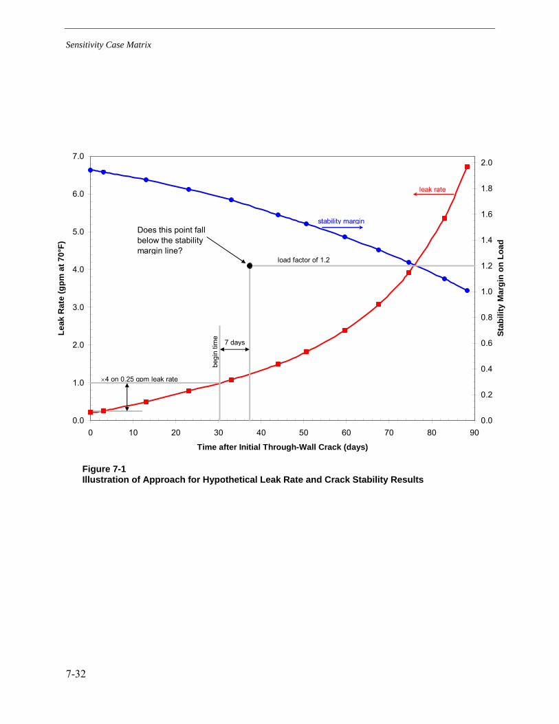
Sensitivity Case Matrix

7-32

0.0

1.0

2.0

3.0

4.0

5.0

6.0

7.0

0 10 20 30 40 50 60 70 80 90

Time after Initial Through-Wall Crack (days)

Leak

Rat

e (g

pm a

t 70°

F)

0.0

0.2

0.4

0.6

0.8

1.0

1.2

1.4

1.6

1.8

2.0

Stab

ility

Mar

gin

on L

oad

7 days

×4 on 0.25 gpm leak rate

stability margin

leak rate

begi

n tim

e

load factor of 1.2

Does this point fall below the stability margin line?

Figure 7-1 Illustration of Approach for Hypothetical Leak Rate and Crack Stability Results

Sensitivity Case Matrix

7-33

y = 1515168.38650x4 - 3679386.65241x3 + 3143956.32984x2 - 952635.91691x + 42800.90186R2 = 0.99155

-80,000

-60,000

-40,000

-20,000

0

20,000

40,000

60,000

80,000

0.0 0.1 0.2 0.3 0.4 0.5 0.6 0.7 0.8 0.9 1.0

Nondimensional Distance from ID, x /t

Axi

al S

tres

s (p

si)

Type 1a-1 (base case) Poly. (Type 1a-1 (base case))

Figure 7-2 WRS Fit for Type 1 Safety and Relief Nozzle Including Effect of Stainless Steel Weld (with normal operating temperature applied)

y = -591849.2769x3 + 1207788.1107x2 - 618169.1311x + 54261.3841R2 = 0.9443

-80,000

-60,000

-40,000

-20,000

0

20,000

40,000

60,000

80,000

0.0 0.1 0.2 0.3 0.4 0.5 0.6 0.7 0.8 0.9 1.0

Nondimensional Distance from ID, x /t

Axi

al S

tres

s (p

si)

Type 1a-3 (no SS Weld) ASME Modified per EMC2 Poly. (Type 1a-3 (no SS Weld))

Figure 7-3 WRS Cubic Fit for Type 1 Safety and Relief Nozzle Excluding Effect of Stainless Steel Weld (with normal operating temperature applied)

Sensitivity Case Matrix

7-34

y = 833566.7025x4 - 2176526.9737x3 + 2124566.3456x2 - 771992.0080x + 54000.0000R2 = 0.9693

-80,000

-60,000

-40,000

-20,000

0

20,000

40,000

60,000

80,000

0.0 0.1 0.2 0.3 0.4 0.5 0.6 0.7 0.8 0.9 1.0

Nondimensional Distance from ID, x /t

Axi

al S

tres

s (p

si)

Type 1a-3 (no SS Weld) ASME Modified per EMC2 Poly. (Type 1a-3 (no SS Weld))

Figure 7-4 WRS Quartic Fit for Type 1 Safety and Relief Nozzle Excluding Effect of Stainless Steel Weld with σ0 set to 54 ksi (with normal operating temperature applied)

y = 368125.90618x3 - 302363.56840x2 - 72263.72562x + 74800.00000R2 = 0.96857

y = -346646.916833x3 + 872630.992358x2 - 487133.355555x + 27500.000000R2 = 0.992444

-60000

-40000

-20000

0

20000

40000

60000

80000

0.0 0.1 0.2 0.3 0.4 0.5 0.6 0.7 0.8 0.9 1.0

Nondimensional Distance from ID, x /t

Axi

al S

tres

s (p

si)

0 20 EQUIV AXI REPAIR Poly. (0) Poly. (20)

Figure 7-5 WRS Fits for Safety and Relief Nozzle with 3D ID Repair Excluding Effect of Stainless Steel Weld with σ0 set to 27.5 ksi and 74.8 ksi (with normal operating temperature applied)

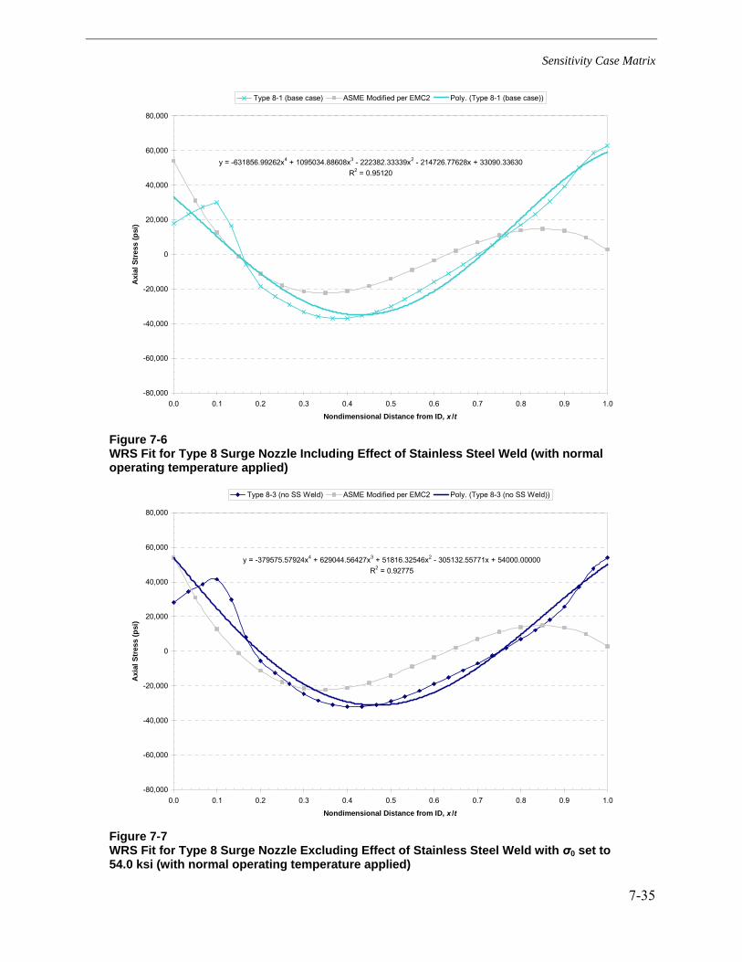
Sensitivity Case Matrix

7-35

y = -631856.99262x4 + 1095034.88608x3 - 222382.33339x2 - 214726.77628x + 33090.33630R2 = 0.95120

-80,000

-60,000

-40,000

-20,000

0

20,000

40,000

60,000

80,000

0.0 0.1 0.2 0.3 0.4 0.5 0.6 0.7 0.8 0.9 1.0

Nondimensional Distance from ID, x /t

Axi

al S

tres

s (p

si)

Type 8-1 (base case) ASME Modified per EMC2 Poly. (Type 8-1 (base case))

Figure 7-6 WRS Fit for Type 8 Surge Nozzle Including Effect of Stainless Steel Weld (with normal operating temperature applied)

y = -379575.57924x4 + 629044.56427x3 + 51816.32546x2 - 305132.55771x + 54000.00000R2 = 0.92775

-80,000

-60,000

-40,000

-20,000

0

20,000

40,000

60,000

80,000

0.0 0.1 0.2 0.3 0.4 0.5 0.6 0.7 0.8 0.9 1.0

Nondimensional Distance from ID, x /t

Axi

al S

tres

s (p

si)

Type 8-3 (no SS Weld) ASME Modified per EMC2 Poly. (Type 8-3 (no SS Weld))

Figure 7-7 WRS Fit for Type 8 Surge Nozzle Excluding Effect of Stainless Steel Weld with σ0 set to 54.0 ksi (with normal operating temperature applied)

Sensitivity Case Matrix

7-36

Figure 7-8 WRS Fit for Type 8 Surge Nozzle Excluding Effect of Stainless Steel Weld (Applied in Case 17b) Compared to DEI and EMC2 WRS FEA Results Including Effect of Stainless Steel Weld

y = -645938.9902617x4 + 796318.7054484x3 - 62420.8136224x2 - 69678.7141941x - 15203.0000000R2 = 0.9463411

-80000

-60000

-40000

-20000

0

20000

40000

60000

80000

0.0 0.1 0.2 0.3 0.4 0.5 0.6 0.7 0.8 0.9 1.0

Nondimensional Distance from ID, x /t

Axi

al S

tres

s (p

si)

Type 9-1 (CE surge) Poly. (Type 9-1 (CE surge))

Figure 7-9 WRS Fit for Type 9 Surge Nozzle Excluding Effect of Stainless Steel Weld with σ0 set to -15.2 ksi (with normal operating temperature applied)

-80,000

-60,000

-40,000

-20,000

0

20,000

40,000

60,000

80,000

0.0 0.1 0.2 0.3 0.4 0.5 0.6 0.7 0.8 0.9 1.0

Nondimensional Distance from ID, x /t

Axi

al S

tres

s (p

si)

Type 8-1 (base case) ASME Modified per EMC2 EMC2 NoRepair-WithSS (Left-Right) Poly. (Type 8-3 (no SS Weld))

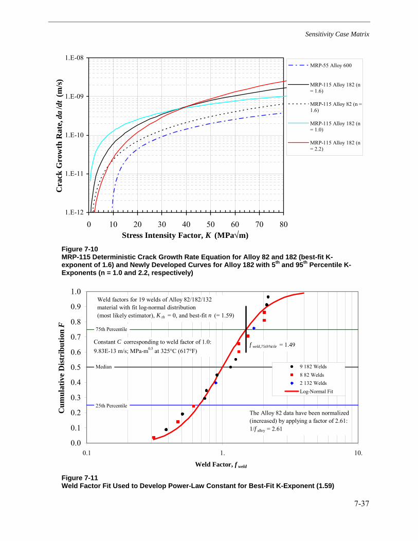
Sensitivity Case Matrix

7-37

1.E-12

1.E-11

1.E-10

1.E-09

1.E-08

0 10 20 30 40 50 60 70 80Stress Intensity Factor, K (MPa√m)

Cra

ck G

row

th R

ate,

da

/dt

(m/s

)MRP-55 Alloy 600

MRP-115 Alloy 182 (n= 1.6)

MRP-115 Alloy 82 (n =1.6)

MRP-115 Alloy 182 (n= 1.0)

MRP-115 Alloy 182 (n= 2.2)

Figure 7-10 MRP-115 Deterministic Crack Growth Rate Equation for Alloy 82 and 182 (best-fit K-exponent of 1.6) and Newly Developed Curves for Alloy 182 with 5th and 95th Percentile K-Exponents (n = 1.0 and 2.2, respectively)

0.0

0.1

0.2

0.3

0.4

0.5

0.6

0.7

0.8

0.9

1.0

0.1 1. 10.

Weld Factor, f weld

Cum

ulat

ive

Dis

trib

utio

n F

9 182 Welds8 82 Welds2 132 WeldsLog-Normal Fit

Weld factors for 19 welds of Alloy 82/182/132material with fit log-normal distribution(most likely estimator), K th = 0, and best-fit n (= 1.59)

25th Percentile

75th Percentile

Median

The Alloy 82 data have been normalized (increased) by applying a factor of 2.61:1/f alloy = 2.61

Constant C corresponding to weld factor of 1.0:9.83E-13 m/s; MPa-m0.5 at 325°C (617°F)

f weld,75th%tile = 1.49

Figure 7-11 Weld Factor Fit Used to Develop Power-Law Constant for Best-Fit K-Exponent (1.59)

Sensitivity Case Matrix

7-38

0.0

0.1

0.2

0.3

0.4

0.5

0.6

0.7

0.8

0.9

1.0

0.1 1. 10.

Weld Factor, f weld

Cum

ulat

ive

Dis

trib

utio

n F

9 182 Welds8 82 Welds2 132 WeldsLog-Normal Fit

Weld factors for 19 welds of Alloy 82/182/132material with fit log-normal distribution(most likely estimator), K th = 0, and assumed n = 1.0

25th Percentile

75th Percentile

Median

The Alloy 82 data have been normalized (increased) by applying a factor of 2.61:1/f alloy = 2.61

Constant C corresponding to weld factor of 1.0:8.75E-12 m/s; MPa-m0.5 at 325°C (617°F) f weld,75th%tile = 1.46

Figure 7-12 Weld Factor Fit Used to Develop Power-Law Constant for 5th Percentile K-Exponent (1.0)

0.0

0.1

0.2

0.3

0.4

0.5

0.6

0.7

0.8

0.9

1.0

0.1 1. 10.

Weld Factor, f weld

Cum

ulat

ive

Dis

trib

utio

n F

9 182 Welds8 82 Welds2 132 WeldsLog-Normal Fit

Weld factors for 19 welds of Alloy 82/182/132material with fit log-normal distribution(most likely estimator), K th = 0, and assumed n = 2.2

25th Percentile

75th Percentile

Median

The Alloy 82 data have been normalized (increased) by applying a factor of 2.61:1/f alloy = 2.61

Constant C corresponding to weld factor of 1.0:1.03E-13 m/s; MPa-m0.5 at 325°C (617°F)

f weld,75th%tile = 1.56

Figure 7-13 Weld Factor Fit Used to Develop Power-Law Constant for 95th Percentile K-Exponent (2.2)

Sensitivity Case Matrix

7-39

-8.0

-6.0

-4.0

-2.0

0.0

2.0

4.0

6.0

8.0

8.0 -6.0 -4.0 -2.0 0.0

Case 17b 7 days after going TW

Case S3b after 1.3 years of growth

Secondary Crack Profile 1 (Case S4b)

Secondary Crack Profile 2 (Case S5b)

Secondary Crack Profile 3 (Case S6b)

Secondary Crack Profile 4 (Case S7b)

Figure 7-14 Profiles of Pairs of Additional Cracks Applied in Stability Calculations for Cases S4b through S7b Based on Case 17b

Sensitivity Case Matrix

7-40

Figure 7-15 Case S9b Growth Progression Based on Individual Growth of Initial 21:1 Aspect Ratio 26% through-wall Flaws Placed at Top and Bottom of Weld Cross Section

-8.0

-6.0

-4.0

-2.0

0.0

2.0

4.0

6.0

8.0

-8.0 -6.0 -4.0 -2.0 0.0

Case S9b after breaking through-wall

Case S9b 7 days after through-wall

Case S9b 12 days after through-wall

Case S9b 25 days after through-wall

Case S9b 35 days after through-wall

Case S9b 42 days after through-wall

Sensitivity Case Matrix

7-41

Figure 7-16 Case S9b Growth Progression Shown in Polar Coordinates

0.0

0.1

0.2

0.3

0.4

0.5

0.6

0.7

0.8

0.9

1.0

0 30 60 90 120 150 180

Circumferential Position, θ (deg)

Non

dim

ensi

onal

Cra

ck D

epth

, y/ t

Case S9b after breaking through-wall

Case S9b 7 days after through-wall

Case S9b 12 days after through-wall

Case S9b 25 days after through-wall

Case S9b 35 days after through-wall

Case S9b 42 days after through-wall

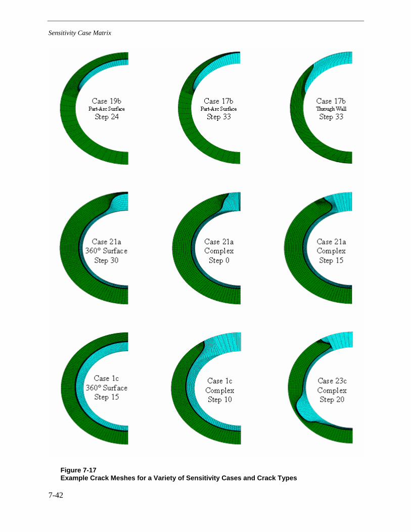
Sensitivity Case Matrix

7-42

Figure 7-17 Example Crack Meshes for a Variety of Sensitivity Cases and Crack Types

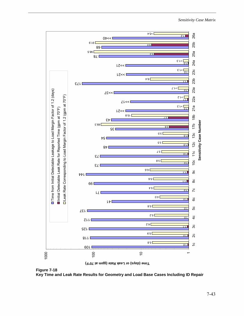
Sensitivity Case Matrix

7-43

Figure 7-18 Key Time and Leak Rate Results for Geometry and Load Base Cases Including ID Repair

109

118

125

112

137

41

71

99

144

73

73

48

54

35

43

>>21

>>17

>>37

173

>>21

>>21

78

68

>>40

1.0

1.0

1.1

1.0

1.0

1.0

1.0

1.1

1.1

1.0

1.0

1.0

1.0

2.6

2.7

1.0

1.1

1.0

1.1

1.0

1.0

5.3

6.0

1.2

5.8

5.9

6.2

5.2

5.8

4.0

5.4

5.6

6.6

3.8

3.7

3.5

3.5

69.3

15.8

>1.3

>1.2

>1.7

6.4

>1.3

>1.3

98.5

91.9

>5.4

110100

1000

1c2c

3c4c

5c6c

7c8c

9c10

c11

c12

c13

c17

b18

b21

a22

a23

a23

b23

c24

a25

a25

b26

a

Sens

itivi

ty C

ase

Num

ber

Time (days) or Leak Rate (gpm at 70°F)Ti

me

from

Initi

al D

etec

tabl

e Le

akag

e to

Loa

d M

argi

n Fa

ctor

of 1

.2 (d

ays)

Initi

al D

etec

tabl

e Le

ak R

ate

for R

epor

ted

Tim

e (g

pm a

t 70°

F)

Leak

Rat

e C

orre

spon

ding

to L

oad

Mar

gin

Fact

or o

f 1.2

(gpm

at 7

0°F)

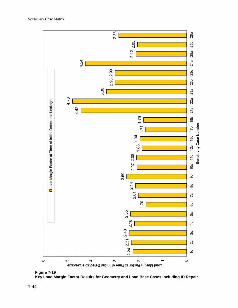
Sensitivity Case Matrix

7-44

Figure 7-19 Key Load Margin Factor Results for Geometry and Load Base Cases Including ID Repair

2.24

2.31

2.40

2.18

2.35

1.70

2.01

2.14

2.50

2.07

2.08

1.86

1.94

1.71

1.79

4.42

4.78

3.36

2.98

2.99

4.24

2.12

2.05

2.83

0123456

1c2c

3c4c

5c6c

7c8c

9c10

c11

c12

c13

c17

b18

b21

a22

a23

a23

b23

c24

a25

a25

b26

a

Sens

itivi

ty C

ase

Num

ber

Load Margin Factor at Time of Initial Detectable Leakage

Load

Mar

gin

Fact

or a

t Tim

e of

Initi

al D

etec

tabl

e Le

akag

e

Sensitivity Case Matrix

7-45

Figure 7-20 Key Time and Leak Rate Results for Other Main Cases

38

27

11

146

74

123

98

32

42

49

49

47

53

44

39

47

37

46

73

22

39

145

293

94

49

2.5

2.4

4.1

1.1

1.0

1.0

1.1

1.1

1.0

1.0

1.0

1.0

1.0

1.0

1.1

1.0

1.0

1.1

4.6

1.4

2.4

1.0

1.1

1.0

2.4

70.4

28.8

8.5

6.4

4.8

5.3

5.5

3.7

4.0

5.0

5.0

4.9

5.2

4.7

3.0

4.8

2.6

3.9

73.6

63.3

70.1

8.6

191.4

6.61

42.35

110100

1000

27b

28b

29b

31c

32c

33c

34c

35c

36c

37c

38c

39c

40c

41c

42c

43c

44c

45c

46b

47b

48b

49c

50b

52c

53b

Sens

itivi

ty C

ase

Num

ber

Time (days) or Leak Rate (gpm at 70°F)

Tim

e fro

m In

itial

Det

ecta

ble

Leak

age

to L

oad

Mar

gin

Fact

or o

f 1.2

(day

s)

Initi

al D

etec

tabl

e Le

ak R

ate

for R

epor

ted

Tim

e (g

pm a

t 70°

F)

Leak

Rat

e C

orre

spon

ding

to L

oad

Mar

gin

Fact

or o

f 1.2

(gpm

at 7

0°F)

Sensitivity Case Matrix

7-46

Figure 7-21 Key Load Margin Factor Results for Other Main Cases

1.74

1.67

1.38

2.46

1.96

2.20

2.12

1.62

1.69

1.83

1.83

1.81

1.89

1.77

1.57

1.84

1.69

1.91

1.71

1.70

1.73

2.85

4.33

2.26

1.69

0123456

27b

28b

29b

31c

32c

33c

34c

35c

36c

37c

38c

39c

40c

41c

42c

43c

44c

45c

46b

47b

48b

49c

50b

52c

53b

Sens

itivi

ty C

ase

Num

ber

Load Margin Factor at Time of Initial Detectable Leakage

Load

Mar

gin

Fact

or a

t Tim

e of

Initi

al D

etec

tabl

e Le

akag

e

Sensitivity Case Matrix

7-47

0.0

1.0

2.0

3.0

4.0

5.0

6.0

7.0

8.0

9.0

10.0

0 10 20 30 40 50 60 70 80 90 100 110 120 130 140 150 160 170 180

Time after Initial Through-Wall Crack (days)

Lea

k R

ate

(gpm

@ 7

0°F)

0.0

0.2

0.4

0.6

0.8

1.0

1.2

1.4

1.6

1.8

2.0

2.2

2.4

2.6

2.8

3.0

Stab

ility

Mar

gin

on L

oad

C06c Leakage

C06c Stability Margin

Load Factor = 1.2

Tim

e at

1 g

pm

Figure 7-22 Leak Rate and Load Margin Factor as a Function of Time—Case 6c

0.0

1.0

2.0

3.0

4.0

5.0

6.0

7.0

8.0

9.0

10.0

0 10 20 30 40 50 60 70 80 90 100 110 120 130 140 150 160 170 180

Time after Initial Through-Wall Crack (days)

Lea

k R

ate

(gpm

@ 7

0°F)

0.0

0.2

0.4

0.6

0.8

1.0

1.2

1.4

1.6

1.8

2.0

2.2

2.4

2.6

2.8

3.0

Stab

ility

Mar

gin

on L

oad

C12c Leakage

C12c Stability Margin

Load Factor = 1.2

Tim

e at

1 g

pm

Figure 7-23 Leak Rate and Load Margin Factor as a Function of Time—Case 12c

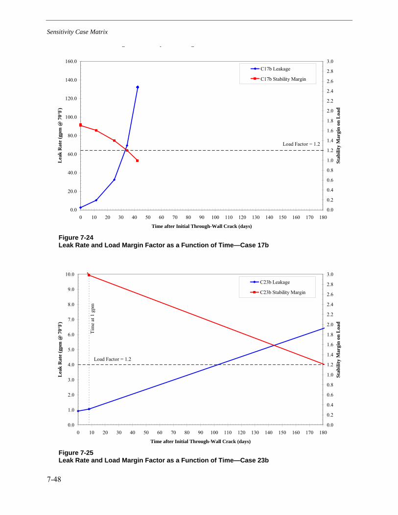
Sensitivity Case Matrix

7-48

Figure 7-24 Leak Rate and Load Margin Factor as a Function of Time—Case 17b

0.0

1.0

2.0

3.0

4.0

5.0

6.0

7.0

8.0

9.0

10.0

0 10 20 30 40 50 60 70 80 90 100 110 120 130 140 150 160 170 180

Time after Initial Through-Wall Crack (days)

Lea

k R

ate

(gpm

@ 7

0°F)

0.0

0.2

0.4

0.6

0.8

1.0

1.2

1.4

1.6

1.8

2.0

2.2

2.4

2.6

2.8

3.0

Stab

ility

Mar

gin

on L

oad

C23b Leakage

C23b Stability Margin

Load Factor = 1.2

Tim

e at

1 g

pm

Figure 7-25 Leak Rate and Load Margin Factor as a Function of Time—Case 23b

g y g

0.0

20.0

40.0

60.0

80.0

100.0

120.0

140.0

160.0

0 10 20 30 40 50 60 70 80 90 100 110 120 130 140 150 160 170 180

Time after Initial Through-Wall Crack (days)

Lea

k R

ate

(gpm

@ 7

0°F)

0.0

0.2

0.4

0.6

0.8

1.0

1.2

1.4

1.6

1.8

2.0

2.2

2.4

2.6

2.8

3.0

Stab

ility

Mar

gin

on L

oad

C17b Leakage

C17b Stability Margin

Load Factor = 1.2

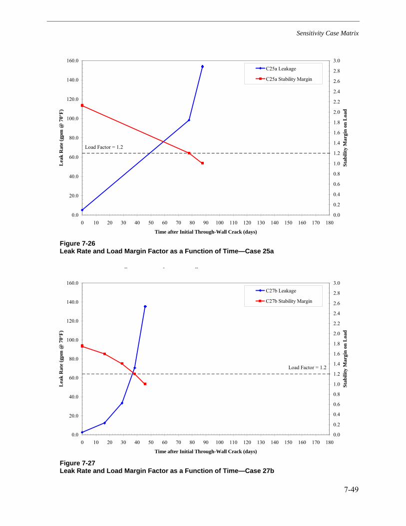
Sensitivity Case Matrix

7-49

0.0

20.0

40.0

60.0

80.0

100.0

120.0

140.0

160.0

0 10 20 30 40 50 60 70 80 90 100 110 120 130 140 150 160 170 180

Time after Initial Through-Wall Crack (days)

Lea

k R

ate

(gpm

@ 7

0°F)

0.0

0.2

0.4

0.6

0.8

1.0

1.2

1.4

1.6

1.8

2.0

2.2

2.4

2.6

2.8

3.0

Stab

ility

Mar

gin

on L

oad

C25a Leakage

C25a Stability Margin

Load Factor = 1.2

Figure 7-26 Leak Rate and Load Margin Factor as a Function of Time—Case 25a

Figure 7-27 Leak Rate and Load Margin Factor as a Function of Time—Case 27b

g y g

0.0

20.0

40.0

60.0

80.0

100.0

120.0

140.0

160.0

0 10 20 30 40 50 60 70 80 90 100 110 120 130 140 150 160 170 180

Time after Initial Through-Wall Crack (days)

Leak

Rat

e (g

pm @

70°

F)

0.0

0.2

0.4

0.6

0.8

1.0

1.2

1.4

1.6

1.8

2.0

2.2

2.4

2.6

2.8

3.0

Stab

ility

Mar

gin

on L

oad

C27b Leakage

C27b Stability Margin

Load Factor = 1.2

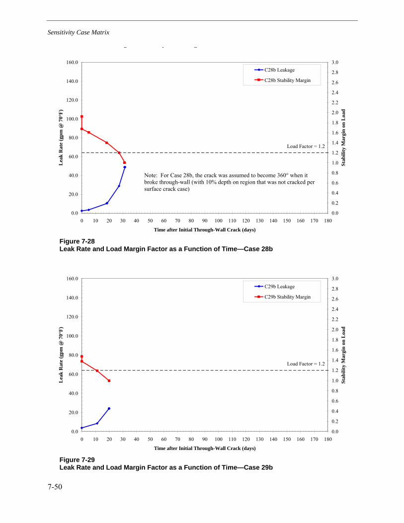
Sensitivity Case Matrix

7-50

Figure 7-28 Leak Rate and Load Margin Factor as a Function of Time—Case 28b

0.0

20.0

40.0

60.0

80.0

100.0

120.0

140.0

160.0

0 10 20 30 40 50 60 70 80 90 100 110 120 130 140 150 160 170 180

Time after Initial Through-Wall Crack (days)

Lea

k R

ate

(gpm

@ 7

0°F)

0.0

0.2

0.4

0.6

0.8

1.0

1.2

1.4

1.6

1.8

2.0

2.2

2.4

2.6

2.8

3.0

Stab

ility

Mar

gin

on L

oad

C29b Leakage

C29b Stability Margin

Load Factor = 1.2

Figure 7-29 Leak Rate and Load Margin Factor as a Function of Time—Case 29b

g y g

0.0

20.0

40.0

60.0

80.0

100.0

120.0

140.0

160.0

0 10 20 30 40 50 60 70 80 90 100 110 120 130 140 150 160 170 180

Time after Initial Through-Wall Crack (days)

Lea

k R

ate

(gpm

@ 7

0°F)

0.0

0.2

0.4

0.6

0.8

1.0

1.2

1.4

1.6

1.8

2.0

2.2

2.4

2.6

2.8

3.0

Stab

ility

Mar

gin

on L

oad

C28b Leakage

C28b Stability Margin

Load Factor = 1.2

Note: For Case 28b, the crack was assumed to become 360° when it broke through-wall (with 10% depth on region that was not cracked per surface crack case)

Sensitivity Case Matrix

7-51

0.0

1.0

2.0

3.0

4.0

5.0

6.0

7.0

8.0

9.0

10.0

0 10 20 30 40 50 60 70 80 90 100 110 120 130 140 150 160 170 180

Time after Initial Through-Wall Crack (days)

Lea

k R

ate

(gpm

@ 7

0°F)

0.0

0.2

0.4

0.6

0.8

1.0

1.2

1.4

1.6

1.8

2.0

2.2

2.4

2.6

2.8

3.0

Stab

ility

Mar

gin

on L

oad

C35c Leakage

C35c Stability Margin

Load Factor = 1.2

Tim

e at

1 g

pm

Figure 7-30 Leak Rate and Load Margin Factor as a Function of Time—Case 35c

Figure 7-31 Leak Rate and Load Margin Factor as a Function of Time—Case 36c

g y g

0.0

1.0

2.0

3.0

4.0

5.0

6.0

7.0

8.0

9.0

10.0

0 10 20 30 40 50 60 70 80 90 100 110 120 130 140 150 160 170 180

Time after Initial Through-Wall Crack (days)

Lea

k R

ate

(gpm

@ 7

0°F)

0.0

0.2

0.4

0.6

0.8

1.0

1.2

1.4

1.6

1.8

2.0

2.2

2.4

2.6

2.8

3.0

Stab

ility

Mar

gin

on L

oad

C36c Leakage

C36c Stability Margin

Load Factor = 1.2

Tim

e at

1 g

pm

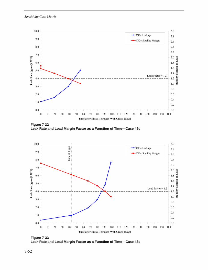
Sensitivity Case Matrix

7-52

0.0

1.0

2.0

3.0

4.0

5.0

6.0

7.0

8.0

9.0

10.0

0 10 20 30 40 50 60 70 80 90 100 110 120 130 140 150 160 170 180

Time after Initial Through-Wall Crack (days)

Lea

k R

ate

(gpm

@ 7

0°F)

0.0

0.2

0.4

0.6

0.8

1.0

1.2

1.4

1.6

1.8

2.0

2.2

2.4

2.6

2.8

3.0

Stab

ility

Mar

gin

on L

oad

C42c Leakage

C42c Stability Margin

Load Factor = 1.2

Figure 7-32 Leak Rate and Load Margin Factor as a Function of Time—Case 42c

0.0

1.0

2.0

3.0

4.0

5.0

6.0

7.0

8.0

9.0

10.0

0 10 20 30 40 50 60 70 80 90 100 110 120 130 140 150 160 170 180

Time after Initial Through-Wall Crack (days)

Lea

k R

ate

(gpm

@ 7

0°F)

0.0

0.2

0.4

0.6

0.8

1.0

1.2

1.4

1.6

1.8

2.0

2.2

2.4

2.6

2.8

3.0

Stab

ility

Mar

gin

on L

oad

C43c Leakage

C43c Stability Margin

Load Factor = 1.2

Tim

e at

1 g

pm

Figure 7-33 Leak Rate and Load Margin Factor as a Function of Time—Case 43c

Sensitivity Case Matrix

7-53

Figure 7-34 Leak Rate and Load Margin Factor as a Function of Time—Case 44c

Figure 7-35 Leak Rate and Load Margin Factor as a Function of Time—Case 46b

g y g

0.0

20.0

40.0

60.0

80.0

100.0

120.0

140.0

160.0

0 10 20 30 40 50 60 70 80 90 100 110 120 130 140 150 160 170 180

Time after Initial Through-Wall Crack (days)

Leak

Rat

e (g

pm @

70°

F)

0.0

0.2

0.4

0.6

0.8

1.0

1.2

1.4

1.6

1.8

2.0

2.2

2.4

2.6

2.8

3.0

Stab

ility

Mar

gin

on L

oad

C46b Leakage

C46b Stability Margin

Load Factor = 1.2

g y g

0.0

1.0

2.0

3.0

4.0

5.0

6.0

7.0

8.0

9.0

10.0

0 10 20 30 40 50 60 70 80 90 100 110 120 130 140 150 160 170 180

Time after Initial Through-Wall Crack (days)

Leak

Rat

e (g

pm @

70°

F)

0.0

0.2

0.4

0.6

0.8

1.0

1.2

1.4

1.6

1.8

2.0

2.2

2.4

2.6

2.8

3.0

Stab

ility

Mar

gin

on L

oad

C44c Leakage

C44c Stability Margin

Load Factor = 1.2Ti

me

at 1

gpm

Sensitivity Case Matrix

7-54

0.0

20.0

40.0

60.0

80.0

100.0

120.0

140.0

160.0

0 10 20 30 40 50 60 70 80 90 100 110 120 130 140 150 160 170 180

Time after Initial Through-Wall Crack (days)

Lea

k R

ate

(gpm

@ 7

0°F)

0.0

0.2

0.4

0.6

0.8

1.0

1.2

1.4

1.6

1.8

2.0

2.2

2.4

2.6

2.8

3.0

Stab

ility

Mar

gin

on L

oad

C47b Leakage

C47b Stability Margin

Load Factor = 1.2

Figure 7-36 Leak Rate and Load Margin Factor as a Function of Time—Case 47b

Figure 7-37 Leak Rate and Load Margin Factor as a Function of Time—Case 48b

g y g

0.0

20.0

40.0

60.0

80.0

100.0

120.0

140.0

160.0

0 10 20 30 40 50 60 70 80 90 100 110 120 130 140 150 160 170 180

Time after Initial Through-Wall Crack (days)

Lea

k R

ate

(gpm

@ 7

0°F)

0.0

0.2

0.4

0.6

0.8

1.0

1.2

1.4

1.6

1.8

2.0

2.2

2.4

2.6

2.8

3.0

Stab

ility

Mar

gin

on L

oad

C48b Leakage

C48b Stability Margin

Load Factor = 1.2

Sensitivity Case Matrix

7-55

0.0

20.0

40.0

60.0

80.0

100.0

120.0

140.0

160.0

0 10 20 30 40 50 60 70 80 90 100 110 120 130 140 150 160 170 180

Time after Initial Through-Wall Crack (days)

Lea

k R

ate

(gpm

@ 7

0°F)

0.0

0.2

0.4

0.6

0.8

1.0

1.2

1.4

1.6

1.8

2.0

2.2

2.4

2.6

2.8

3.0

Stab

ility

Mar

gin

on L

oad

C53b Leakage

C53b Stability Margin

Load Factor = 1.2

Figure 7-38 Leak Rate and Load Margin Factor as a Function of Time—Case 53b

Figure 7-39 Leak Rate and Load Margin Factor as a Function of Time—Case S1b

g y g

0.0

20.0

40.0

60.0

80.0

100.0

120.0

140.0

160.0

0 10 20 30 40 50 60 70 80 90 100 110 120 130 140 150 160 170 180

Time after Initial Through-Wall Crack (days)

Lea

k R

ate

(gpm

@ 7

0°F)

0.0

0.2

0.4

0.6

0.8

1.0

1.2

1.4

1.6

1.8

2.0

2.2

2.4

2.6

2.8

3.0

Stab

ility

Mar

gin

on L

oad

S1b Leakage

S1b Stability Margin

Load Factor = 1.2

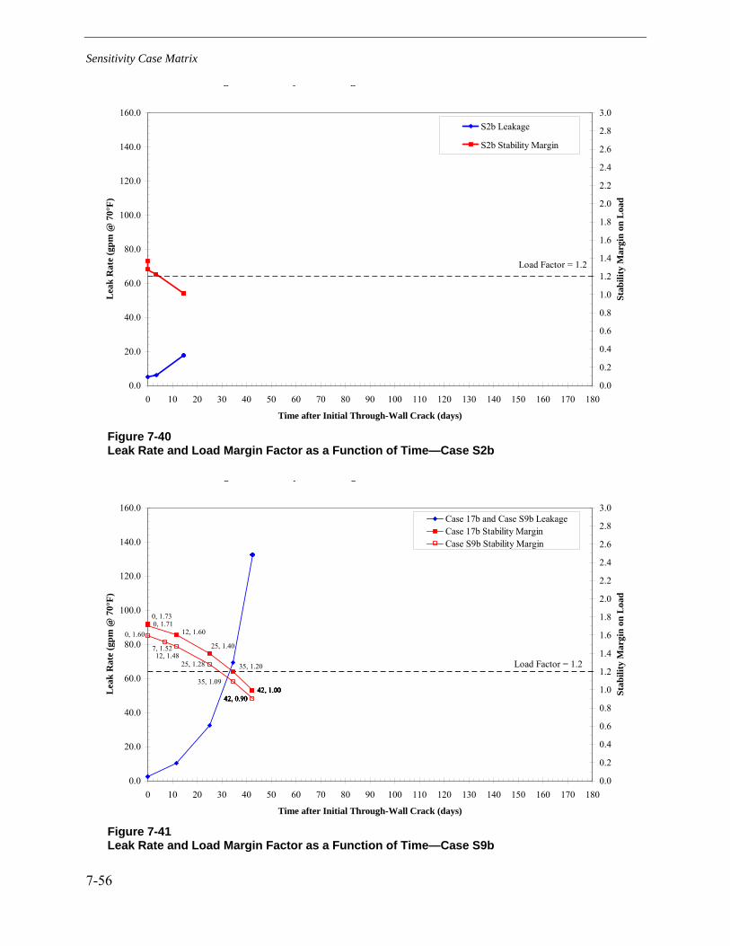
Sensitivity Case Matrix

7-56

Figure 7-40 Leak Rate and Load Margin Factor as a Function of Time—Case S2b

Figure 7-41 Leak Rate and Load Margin Factor as a Function of Time—Case S9b

g y g

42, 1.0042, 1.0042, 1.0042, 1.0042, 1.00

25, 1.28

42, 0.9042, 0.9042, 0.9042, 0.9042, 0.90

0, 1.73

25, 1.40

12, 1.60

35, 1.20

0, 1.71

35, 1.09

0, 1.60

7, 1.5212, 1.48

0.0

20.0

40.0

60.0

80.0

100.0

120.0

140.0

160.0

0 10 20 30 40 50 60 70 80 90 100 110 120 130 140 150 160 170 180

Time after Initial Through-Wall Crack (days)

Leak

Rat

e (g

pm @

70°

F)

0.0

0.2

0.4

0.6

0.8

1.0

1.2

1.4

1.6

1.8

2.0

2.2

2.4

2.6

2.8

3.0

Stab

ility

Mar

gin

on L

oad

Case 17b and Case S9b LeakageCase 17b Stability MarginCase S9b Stability Margin

Load Factor = 1.2

g y g

0.0

20.0

40.0

60.0

80.0

100.0

120.0

140.0

160.0

0 10 20 30 40 50 60 70 80 90 100 110 120 130 140 150 160 170 180

Time after Initial Through-Wall Crack (days)

Leak

Rat

e (g

pm @

70°

F)

0.0

0.2

0.4

0.6

0.8

1.0

1.2

1.4

1.6

1.8

2.0

2.2

2.4

2.6

2.8

3.0

Stab

ility

Mar

gin

on L

oad

S2b Leakage

S2b Stability Margin

Load Factor = 1.2

8-1

8 SUMMARY AND CONCLUSIONS

A summary of the findings of this study, including main conclusions, are as follows:

• ELIMINATION OF OVERLY CONSERVATIVE ASSUMPTION OF SEMI-ELLIPTICAL CRACK SHAPE. A calculation methodology has been developed through extensions to the FEACrack software to model the shape progression of a circumferential PWSCC flaw based on the stress intensity factor calculated at each point on the crack front. This refinement in crack growth modeling eliminates the need to assume that the crack shape remains a semi-ellipse grown on the basis of the stress intensity factor at the deepest and surface points. This study demonstrates that this classical assumption of a semi-elliptical crack shape results in a large overestimation of the crack area and thus underestimation of the crack stability at the point in time at which the crack penetrates to the outside surface.

• COLLECTION OF PLANT-SPECIFIC INPUTS. Extensive weld-specific design and fabrication inputs were collected for the group of 51 subject dissimilar metal welds. Detailed geometry and piping load inputs were collected for each subject weld to ensure that all welds are appropriately addressed by the crack growth sensitivity matrix developed as part of this study. Weld-specific fabrication and weld repair data were also collected as a key input to the welding residual stress simulations addressing the subject population. The frequency of ID weld repairs in the subject population was found to be significantly less than that for the Wolf Creek pressurizer nozzle dissimilar metal welds.

• WELDING RESIDUAL STRESS SIMULATIONS. A matrix of welding residual stress (WRS) simulations were performed on the basis of the detailed design, fabrication, and weld repair information collected. Axisymmetric and non-axisymmetric weld repair WRS profiles were developed for input to the crack growth simulations under various assumptions in recognition of the uncertainty in calculation of WRS values. In addition, the WRS methodology applied in this report was benchmarked versus stress measurements and the simulations of other organizations for a piping butt weld mockup.

• CRITICAL CRACK SIZE METHODOLOGY. A critical crack size methodology was developed specific to the subject nozzle-to-safe-end geometry and materials. This methodology, which was implemented as a post-processing calculation to the crack profiles simulated in the crack growth calculations, is based on the net section collapse (NSC) equations for an arbitrary circumferential crack profile in a thin-walled pipe. Although new calculations and past experimental experience indicate that secondary piping thermal constraint loads will significantly or completely relax prior to rupture, normal thermal piping loads were included in the crack stability calculations. In addition, a Z-factor approach reducing the NSC failure load was implemented in consideration of the possibility of an EPFM failure mechanism. Available experimental failure data for complex cracks in materials similar to Alloy 82/182

Summary and Conclusions

8-2

show that the implemented critical crack size methodology likely results in conservative predictions of rupture.

• LEAK RATE METHODOLOGY. EPRI’s PICEP software was applied to calculate the leak rate development for the simulated through-wall and complex crack profiles. The crack opening area at the weld OD calculated in the crack growth finite-element simulations was applied directly in these PICEP leak rate calculations. NRC’s SQUIRT software was also applied in scoping leak rate calculations, and was found to predict slightly higher leak rates (that would be identified sooner) than PICEP.

• DEVELOPMENT OF EVALUATION CRITERIA. Based on the detailed input of the EPRI expert panel, a set of criteria were developed to evaluate the results of the crack growth, crack stability, and leak rate calculations for each sensitivity case investigated. These criteria provide guidance for applying the matrix results, and were developed in consideration of the many modeling uncertainties addressed in the detailed calculations performed. The evaluation criteria provide safety margins based on explicit consideration of leak rate detection sensitivity, plant response time, and uncertainty in the crack stability calculations.

• CRACK GROWTH SENSITIVITY MATRIX DEVELOPMENT. An extensive sensitivity matrix of 119 cases was developed to robustly address the weld-specific geometry and load input parameters for the set of 51 subject welds, plus key modeling uncertainties such as those associated with WRS, initial crack shape and depth, the K-dependence of the crack growth rate equation, and the effect of multiple flaws. The later cases in the sensitivity matrix were defined to further investigate cases showing limiting results.

• CRACK GROWTH SENSITIVITY MATRIX RESULTS. All 109 cases in the main sensitivity matrix showed either stable crack arrest (60 cases) or crack leakage and crack stability results satisfying the evaluation criteria (49 cases). In most cases, the results showed large evaluation margins in leakage time and in crack stability. The margins in the matrix results demonstrate that even cases representing an unlikely combination of detrimental factors are likely to result in sufficient time for leak detection prior to rupture. The complementary probabilistic evaluations presented in Appendix E further support the adequacy of the deterministic sensitivity cases investigated. Ten supplemental cases were added to further investigate the potential effect of multiple flaws in the subject surge nozzles. Conservative application of the three indications found in the Wolf Creek surge nozzle weld for surge nozzles with a fill-in weld and relatively high moment load gives results meeting the evaluation criteria with additional margin. In addition, considering a case with two long initial partial-arc flaws covering 46% of the ID circumference as opposed to a single initial flaw covering half this circumferential extent (and centered at the location of maximum axial bending stress) has only a modest effect on crack stability for these limiting surge nozzles. On this basis, it is concluded that the concern for multiple flaws in the limiting surge nozzles is adequately addressed by those supplemental cases that satisfy the evaluation criteria with additional margin. In summary, all 51 subject welds are adequately covered by crack growth sensitivity cases that satisfy the evaluation criteria presented in Section 7.2.

Summary and Conclusions

8-3

• TENDENCY OF CIRCUMFERENTIAL SURFACE CRACKS TO SHOW ARREST. An additional key finding concerns the significant number of crack growth sensitivity cases that showed stable crack arrest prior to through-wall penetration. This type of behavior is consistent with the relatively narrow band of relative depths reported for the four largest Wolf Creek indications (23%, 25%, 26%, and 31% through-wall). It is statistically unlikely that these four indications would be found in this narrow depth band if they were in fact growing rapidly in the depth direction at the time they were detected. The basic reason that circumferential cracks may tend to arrest prior to through-wall penetration is that to the extent the through-wall welding residual stress profile is axisymmetric, it must be self-balanced at a particular circumferential position, meaning that a significant portion of the wall thickness must have compressive axial welding residual stresses.

• LARGE BENEFIT GIVEN RELAXATION OF SECONDARY LOADS UPON THROUGH-WALL PENETRATION. Two sensitivity cases showed a greatly increased time between a leak rate of 1.0 gpm and the load margin factor of 1.2 being reached when it is assumed that the piping thermal constraint loads are relieved upon through-wall penetration. These cases confirm the expectation of a large benefit if the piping thermal constraint loads are significantly relaxed once the crack grows through-wall. Detailed evaluations tend to support this kind of behavior, but such relaxation was conservatively not credited in the base assumptions of the critical crack size methodology developed for this study. Rather, 100% of the normal operating thermal piping loads (excluding surge line thermal stratification effects) were included in the critical crack size calculations.

In summary, this study demonstrates the viability of leak detection to preclude the potential for rupture for the pressurizer nozzle dissimilar metal (DM) welds in the group of subject PWRs.

9-1

9 REFERENCES

1. “Implications of Wolf Creek Pressurizer Butt Weld Indications Relative to Safety Assessment and Inspection Requirements,” MRP 2007-003 Attachment 1, January 2007.

2. US NRC, “NRC Wolf Creek Flaw Evaluation,” presented at November 30, 2006, public meeting between US NRC and MRP, North Bethesda, Maryland.

3. US NRC, “Safety Concerns Regarding Potential Pressurizer Weld Cracking,” presented at December 20, 2006, public meeting between US NRC and MRP, Rockville, Maryland.

4. “Review and Refinement of NRC Crack Growth Calculation for Relief Nozzle,” Section 5 in Implications of Wolf Creek Pressurizer Butt Weld Indications Relative to Safety Assessment and Inspection Requirements, MRP 2007-003 Attachment 1, January 2007.

5. “Westinghouse Data: Repair History, Nozzle Dimensions, Nozzle Loads,” Westinghouse Electric Co., NSD-EPRI-07-28, April 27, 2007.

6. “Transmittal of PWROG Information under PA-MSC-0233 to EPRI to Support the Industry Finite Element Analysis (FEA) for the Pressurizer Nozzles, LTR-PCAM-07-38, Rev 1, April 2007,” PWR Owners Group, OG-07-185, April 27, 2007.

7. “Westinghouse and Combustion Engineering Pressurizer Nozzle Fabrication Detail,” Westinghouse Electric Co., NSD-EPRI-07-41, July 27, 2007.

8. “Transmittal of Final PWROG Information under PA-MSC-0233 to EPRI to Support the Industry Finite Element Analysis (FEA) for the Pressurizer Nozzles, LTR-PCAM-07-67, July 20, 2007,” PWR Owners Group, OG-07-343, July 26, 2007.

9. Modeling and Meshing Guide, ANSYS 10.0 Documentation, ANSYS, Inc.

10. Inconel Alloy 600, Special Metals Corporation Publication No. SMC 027, September 2002.

11. ASME Boiler and Pressure Vessel Code, Section II, Part D, Properties, 1992 Edition.

12. M. H. Duc, “Specification de Calcul de Maquettes d'adaptateurs.” EdF Specification MS-92-090-A-GPE: A667M.

References

9-2

13. L. Karlsson, M. Jonsson, L-E. Lindgren, M. Näsström, and L. Troive, “Residual Stresses and Deformations in a Welded Thin-Walled Pipe.”, ASME Pressure Vessels & Piping Conference, Honolulu, Hawaii, USA, July 1989.

14. E. F. Rybicki and R. B. Stonesifer, “Computation of Residual Stresses due to Multipass Welds in Piping Systems,” Journal of Pressure Vessel Technology, Volume 101, May 1979, pp. 149-154.

15. BWR Vessel and Internals Project: Evaluation of Crack Growth in BWR Stainless Steel RPV Internals (BWRVIP-14), EPRI No. TR-105873, Appendix H. Palo Alto, CA: Electric Power Research Institute, March 1996.

16. “Welding Handbook,” Volume One, Seventh Edition, p. 94, American Welding Society, 1981.

17. P. Dong, J. Zhang, and P. J. Bouchard, “Effects of Repair Weld Length on Residual Stress Distribution,” Journal of Pressure Vessel Technology, vol. 124, February 2002.

18. T. McGaughy and L. Boyles, “Significance of Changes in Residual Stresses and Fracture Toughness due to SMAW Repair of Girth Welds in Line Pipe,” Pipeline Technology Conference, Oostende, Belgium, vol. 2., pp. 16.29-16.36, 1990.

19. Assessment of Dissimilar Metal Weld Integrity: Final Report of the NESC-III Project, EUR 22510 EN, European Commission Joint Research Centre, 2006.

20. NESC-III Project, TG6 2nd (Detailed) Computational Round Robin, NESCDOC TG6 (04) 01, Rev. 2, February 26, 2004.

21. Materials Reliability Program (MRP) Crack Growth Rates for Evaluating Primary Water Stress Corrosion Cracking (PWSCC) of Alloy 82, 182, and 132 Welds (MRP-115), EPRI, Palo Alto, CA: 2004. 1006696.

22. Materials Handbook for Nuclear Plant Pressure Boundary Applications, EPRI, Palo Alto, CA: 2002. 1002792.

23. P. Riccardella, Private Communication to G. White, May 25, 2007.

24. S. Rahman, G. Wilkowski, “Net-Section-Collapse Analysis of Circumferentially Cracked Cylinders—Part I: Arbitrary-Shaped Cracks and Generalized Equations,” Engineering Fracture Mechanics, Vol. 61, pp. 191-211, 1998.

25. G. Wilkowski, H. Xu, D.-J. Shim, and D. Rudland, “Determination of the Elastic-Plastic Fracture Mechanics Z-factor for Alloy 82/182 Weld Metal Flaws for Use in the ASME Section XI Appendix C Flaw Evaluation Procedures,” PVP2007-26733, Proceedings of ASME-PVP 2007: 2007 ASME Pressure Vessels and Piping Division Conference, San Antonio, TX, 2007.

References

9-3

26. G. Wilkowski, H. Xu, P. Krishnaswamy, N. Chokshi, S. Shaukat, A. Hiser, G. Degrassi, J. Johnson, and R. Olson, “Seismic Considerations for the Transition Break Size,” PVP2006-ICPVT11-93994, Proceedings of ASME-PVP 2006 Pressure Vessels and Piping Division Conference, 2006, Vancouver, BC, Canada.

27. D. S. Kupperman, S. H. Sheen, W. J. Shack, D. R. Diercks, P. Krishnaswamy, D. Rudland, and G. M. Wilkowski, “Barrier Integrity Research Program: Final Report,” NUREG/CR-6861, December 2004.

28. ANSC for Determining Net Section Collapse of Arbitrarily Thinned Cylinder, Software User Manual, Structural Integrity Associates, San Jose, CA: 1994.

29. An Assessment of Circumferentially Complex-Cracked Pipe Subjected to Bending, Battelle, Columbus, OH, 1986. NUREG/CR-4687.

30. Fracture Analysis of Welded Type 304 Stainless Steel Pipe: J-R Curve Characterization and Limit Load Analysis, David W. Taylor Naval Ship Research and Development Center, Bethesda, MD, 1986. NUREG/CR-4538-V1.

31. Instability Predictions for Circumferentially Cracked Type-304 Stainless Steel Pipes Under Dynamic Loading, EPRI, Palo Alto, CA: 1982. NP-2347 Volumes 1 and 2.

32. PICEP: Pipe Crack Evaluation Program (Revision 1), EPRI, Palo Alto, CA: 1987. NP-3596-SR.

33. D. Rudland, R. Wolterman, G. Wilkowski, R. Tregoning, “Impact of PWSCC and Current Leak Detection on Leak-Before-Break,” Vessel Head Penetration Inspection, Cracking, and Repairs Conference, Gaithersburg, MD, 2003.

34. SQUIRT Computer Code: Windows Version 1.1 User’s Manual, Battelle, Columbus, OH, 2003. NRC-04-91-063.

35. US NRC, Standard Review Plan, 3.6.3 Leak-Before-Break Evaluation Procedures, NUREG-0800, Revision 1, March 2007.

36. T. Sullivan and A. Csontos, “NRC Questions and Comments on the Industry Advanced FEA Draft Report,” July 12, 2007.

37. B. Brust and P. Scott, “Battelle Memorial Lab Results: EU Report WRS Round Robin Study Modeling,” presented at MRP-NRC meeting of July 12, 2007.

38. T. L. Anderson, Fracture Mechanics, Third Edition, CRC Press, Taylor & Francis Group, New York, 2005, pp. 86-87.

39. T. L. Anderson, et al., “Development of Stress Intensity Factor Solutions for Surface and Embedded Cracks In API 579,” Welding Research Council Bulletin 471, May 2002.

References

9-4

40. R. Bandy and D. van Rooyan, “Quantitative Examination of Stress Corrosion Cracking of Alloy 600 in High Temperature Water – Work in 1983,” Proceedings: 1983 EPRI Workshop on Primary-Side Stress Corrosion Cracking of PWR Steam Generator Tubing, EPRI, Palo Alto, CA: 1987. NP-5498.

41. Analysis of Stress Corrosion Cracks in Alloy 182 Weld Metal After Exposure to PWR Primary Water (MRP-107), EPRI, Palo Alto, CA: 2004. 1009399.

A-1

A APPENDIX A: DISSIMILAR METAL BUTT WELD FABRICATION PROCESSES

Appendix A was prepared by

Westinghouse Electric Co. Nuclear Services 4350 Northern Pike Monroeville, PA 15146

Principal Investigator C. Martin

A.1 General Pressurizer Nozzle Fabrication Processes

This section outlines the general fabrication processes used in production of the dissimilar metal (DM) butt welds of the Combustion Engineering and Westinghouse designed pressurizer surge, spray, safety, and relief nozzles. This section only applies to the subject plants and was created by reviewing design and fabrication information. For the subject plants either a machining or back-welding process was used to ensure solid weld metal throughout the DM weld region. Table A-1 outlines the applicable fabrication process for the subject DM weld locations.

The following provides a brief overview of the three “DM welding processes” noted in Table A-1. A more detailed discussion of these processes is then provided in Section A.2. The fabrication overview will focus on the surge nozzle, but many details of the fabrication process apply equally to the safety/relief nozzles and to the spray nozzles.

1. MACHINED DM WELD LAND WITH ROLLED THERMAL SLEEVE (Figure A-1). Following initial DM weldout, the nozzle DM weld preparation (i.e. weld land) and the inside diameter (ID) of the safe-end were machined to final dimensions. During the machining process the DM weld lands and DM root pass weld were removed to ensured solid weld metal in the DM weld region. The thermal sleeve for the surge and spray nozzles were installed using a rolling process only (no welding).

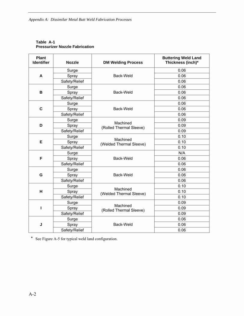
Appendix A: Dissimilar Metal Butt Weld Fabrication Processes

A-2

Table A-1 Pressurizer Nozzle Fabrication

Plant Identifier Nozzle DM Welding Process

Buttering Weld Land Thickness (inch)*

Surge 0.06 Spray 0.06 A

Safety/Relief Back-Weld

0.06 Surge 0.06 Spray 0.06 B

Safety/Relief Back-Weld

0.06 Surge 0.06 Spray 0.06 C

Safety/Relief Back-Weld

0.06 Surge 0.09 Spray 0.09 D

Safety/Relief

Machined (Rolled Thermal Sleeve)

0.09 Surge 0.10 Spray 0.10 E

Safety/Relief

Machined (Welded Thermal Sleeve)

0.10 Surge N/A Spray 0.06 F

Safety/Relief Back-Weld

0.06 Surge 0.06 Spray 0.06 G

Safety/Relief Back-Weld

0.06 Surge 0.10 Spray 0.10 H

Safety/Relief

Machined (Welded Thermal Sleeve)

0.10 Surge 0.09 Spray 0.09 I

Safety/Relief

Machined (Rolled Thermal Sleeve)

0.09 Surge 0.06 Spray 0.06 J

Safety/Relief Back-Weld

0.06

* See Figure A-5 for typical weld land configuration.

Appendix A: Dissimilar Metal Butt Weld Fabrication Processes

A-3

Figure A-1 Surge Nozzle – Machined DM Weld with Rolled Thermal Sleeve

2. BACK-WELD DM WELD LAND WITH WELDED THERMAL SLEEVE (Figure A-2). Following initial DM weldout, the ID DM weld preparation (i.e. weld land) was removed using a grinding process (nozzle ID, 360 degrees circumference). To ensure that the excavation reached the proper depth a dye penetrant examination was used to ensure the weld lands of the nozzle buttering and the safe-end were removed to sound metal. The resultant excavation was then back-welded using Alloy 182, which ensured solid weld metal throughout the DM weld region. Upon completion of the back-welding process an ID weld buildup (thermal sleeve fill-in weld) was applied, at the DM weld, in preparation for the installation of the thermal sleeve. Before the thermal sleeve was installed the weld buildup was machined and PT examined. Following a rolling process an Alloy 82/182 weld, for 45 degrees of the circumference, is used to attach the thermal sleeve to the safe end.

Thermal Sleeve

Weld Buttering

Surge Nozzle

Safe- End

DM Weld

Surge Nozzle

Safe- End

Appendix A: Dissimilar Metal Butt Weld Fabrication Processes

A-4

Figure A-2 Surge Nozzle – Back-Grooved DM Weld with Welded Thermal Sleeve

3. MACHINED DM WELD LAND WITH WELDED THERMAL SLEEVE (Figure A-3). Following initial DM weldout, the nozzle DM weld preparation (i.e. weld land) and the inside diameter (ID) of the safe-end were machined to final dimensions. During the machining process the DM weld lands were removed, which ensured solid weld metal within the DM weld region. During the machining process the ID of the nozzle is prepared for the installation of the thermal sleeve. Following a rolling process an Alloy 82/182 weld, for 45 degrees of the circumference, is used to attach the thermal sleeve to the safe-end.

Safe- End Nozzle

Weld Buttering DM Weld Back- Weld

Thermal Sleeve Fill-In Weld

Thermal Sleeve Surge Nozzle

Safe- End

Thermal Sleeve Attachment Weld

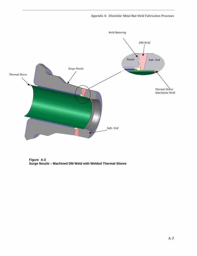
Appendix A: Dissimilar Metal Butt Weld Fabrication Processes

A-5

Figure A-3 Surge Nozzle – Machined DM Weld with Welded Thermal Sleeve

Thermal Sleeve

Surge Nozzle

Weld Buttering

DM Weld

Thermal Sleeve Attachment Weld

Safe- End

Safe- End Nozzle

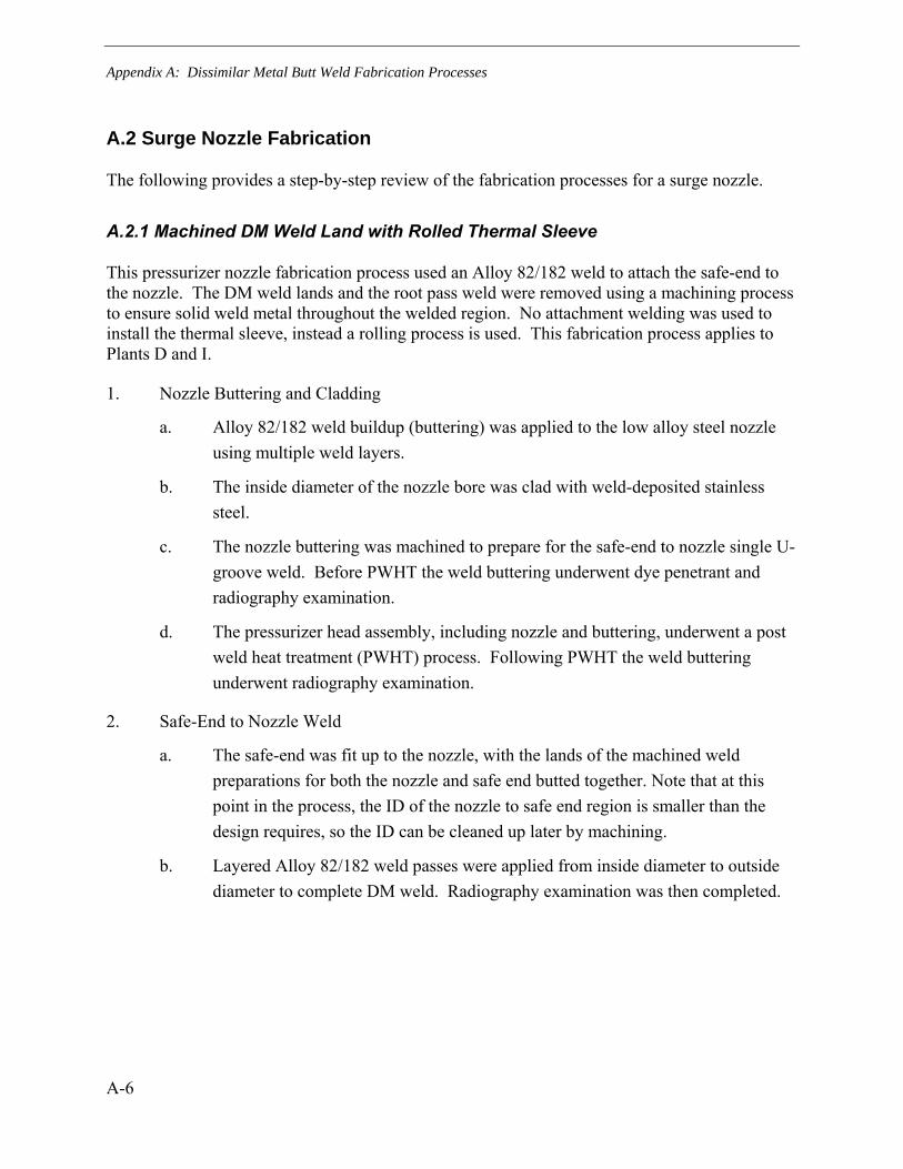
Appendix A: Dissimilar Metal Butt Weld Fabrication Processes

A-6

A.2 Surge Nozzle Fabrication

The following provides a step-by-step review of the fabrication processes for a surge nozzle.

A.2.1 Machined DM Weld Land with Rolled Thermal Sleeve

This pressurizer nozzle fabrication process used an Alloy 82/182 weld to attach the safe-end to the nozzle. The DM weld lands and the root pass weld were removed using a machining process to ensure solid weld metal throughout the welded region. No attachment welding was used to install the thermal sleeve, instead a rolling process is used. This fabrication process applies to Plants D and I.

1. Nozzle Buttering and Cladding

a. Alloy 82/182 weld buildup (buttering) was applied to the low alloy steel nozzle using multiple weld layers.

b. The inside diameter of the nozzle bore was clad with weld-deposited stainless steel.

c. The nozzle buttering was machined to prepare for the safe-end to nozzle single U-groove weld. Before PWHT the weld buttering underwent dye penetrant and radiography examination.

d. The pressurizer head assembly, including nozzle and buttering, underwent a post weld heat treatment (PWHT) process. Following PWHT the weld buttering underwent radiography examination.

2. Safe-End to Nozzle Weld

a. The safe-end was fit up to the nozzle, with the lands of the machined weld preparations for both the nozzle and safe end butted together. Note that at this point in the process, the ID of the nozzle to safe end region is smaller than the design requires, so the ID can be cleaned up later by machining.

b. Layered Alloy 82/182 weld passes were applied from inside diameter to outside diameter to complete DM weld. Radiography examination was then completed.

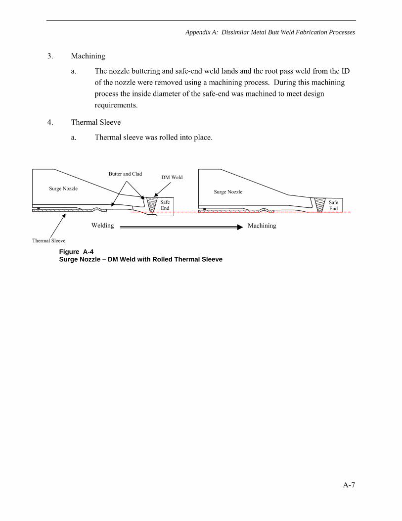
Appendix A: Dissimilar Metal Butt Weld Fabrication Processes

A-7

3. Machining

a. The nozzle buttering and safe-end weld lands and the root pass weld from the ID of the nozzle were removed using a machining process. During this machining process the inside diameter of the safe-end was machined to meet design requirements.

4. Thermal Sleeve

a. Thermal sleeve was rolled into place.

Figure A-4 Surge Nozzle – DM Weld with Rolled Thermal Sleeve

Welding Machining

Thermal Sleeve

Surge Nozzle

Safe End

Butter and Clad DM Weld

Surge Nozzle Safe

End

Appendix A: Dissimilar Metal Butt Weld Fabrication Processes

A-8

A.2.3 Back-Weld DM Weld Land with Welded Thermal Sleeve

This fabrication process used an Alloy 82/182 weld to attach the safe-end to the nozzle. The DM weld lands and a portion of the root pass weld were removed using a back-welding process (Step 3) to ensure solid weld metal throughout the welded region. This fabrication process applies to Plants A, B, C, F, G, and J

1. Nozzle Buttering and Cladding (Figure A-5)

a. Alloy 82/182 weld buildup (buttering) was applied to the low alloy steel nozzle using multiple weld layers.

b. The inside diameter of the nozzle bore was clad with weld-deposited stainless steel.

c. An Alloy 82/182 “tie-in” weld was used to connect the buttering and cladding.

d. The nozzle buttering was machined to prepare for the safe-end to nozzle single U-groove weld (Table A-2). Before PWHT the weld buttering underwent dye penetrant and radiography examination.

e. The pressurizer head assembly, including nozzle and buttering, underwent a post weld heat treatment process. Following PWHT the weld buttering underwent radiography examination.

Table A-2 Clad and Buttering Design

Dimensions

Plant Identifier “A”

(inch)1

A 0.06 B 0.06 C 0.06 D - - - - E - - - -

F 2 0.06 G 0.06 H - - - - I - - - -

J 0.06 Figure A-5 Clad and Buttering

1 – Values also apply to the safety, relief, and spray nozzles.

2 - Surge nozzle DM weld mitigated.

Surge Nozzle

a. Alloy 82/182 Weld Buttering

b. Stainless Steel Cladding

c. Cladding to Buttering Tie-In Weld Alloy 82/182

“A” (Design)

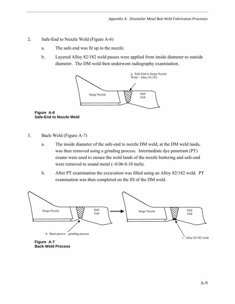
Appendix A: Dissimilar Metal Butt Weld Fabrication Processes

A-9

2. Safe-End to Nozzle Weld (Figure A-6)

a. The safe-end was fit up to the nozzle.

b. Layered Alloy 82/182 weld passes were applied from inside diameter to outside diameter. The DM weld then underwent radiography examination.

Figure A-6 Safe-End to Nozzle Weld

3. Back-Weld (Figure A-7)

a. The inside diameter of the safe-end to nozzle DM weld, at the DM weld lands, was then removed using a grinding process. Intermediate dye penetrant (PT) exams were used to ensure the weld lands of the nozzle buttering and safe-end were removed to sound metal (~0.06-0.10 inch).

b. After PT examination the excavation was filled using an Alloy 82/182 weld. PT examination was then completed on the ID of the DM weld.

Figure A-7 Back-Weld Process

Surge Nozzle

Safe End

h. Back-groove – grinding process

Surge Nozzle

Surge Nozzle

Safe End

Safe End

g. Safe-End to Surge Nozzle Weld – Alloy 82/182.

i. Alloy 82/182 weld

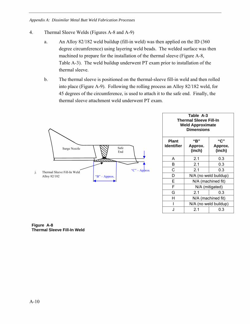
Appendix A: Dissimilar Metal Butt Weld Fabrication Processes

A-10

4. Thermal Sleeve Welds (Figures A-8 and A-9)

a. An Alloy 82/182 weld buildup (fill-in weld) was then applied on the ID (360 degree circumference) using layering weld beads. The welded surface was then machined to prepare for the installation of the thermal sleeve (Figure A-8, Table A-3). The weld buildup underwent PT exam prior to installation of the thermal sleeve.

b. The thermal sleeve is positioned on the thermal-sleeve fill-in weld and then rolled into place (Figure A-9). Following the rolling process an Alloy 82/182 weld, for 45 degrees of the circumference, is used to attach it to the safe end. Finally, the thermal sleeve attachment weld underwent PT exam.

Table A-3

Thermal Sleeve Fill-In Weld Approximate

Dimensions

Plant Identifier

“B” Approx. (inch)

“C” Approx. (inch)

A 2.1 0.3 B 2.1 0.3 C 2.1 0.3 D N/A (no weld buildup) E N/A (machined fit) F N/A (mitigated) G 2.1 0.3 H N/A (machined fit) I N/A (no weld buildup) J 2.1 0.3

Figure A-8 Thermal Sleeve Fill-In Weld

Surge Nozzle

Safe End

j. Thermal Sleeve Fill-In Weld Alloy 82/182 “B” – Approx.

“C” – Approx

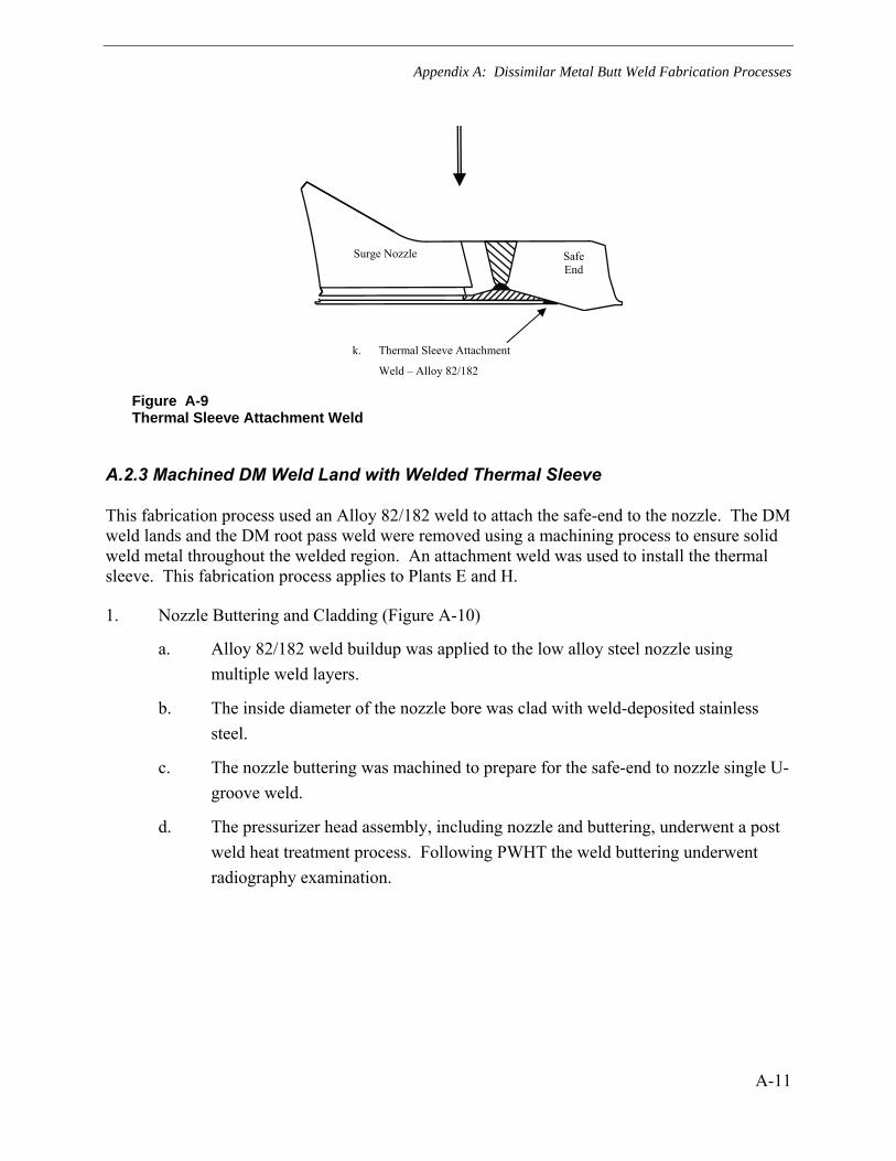
Appendix A: Dissimilar Metal Butt Weld Fabrication Processes

A-11

Figure A-9 Thermal Sleeve Attachment Weld

A.2.3 Machined DM Weld Land with Welded Thermal Sleeve

This fabrication process used an Alloy 82/182 weld to attach the safe-end to the nozzle. The DM weld lands and the DM root pass weld were removed using a machining process to ensure solid weld metal throughout the welded region. An attachment weld was used to install the thermal sleeve. This fabrication process applies to Plants E and H.

1. Nozzle Buttering and Cladding (Figure A-10)

a. Alloy 82/182 weld buildup was applied to the low alloy steel nozzle using multiple weld layers.

b. The inside diameter of the nozzle bore was clad with weld-deposited stainless steel.

c. The nozzle buttering was machined to prepare for the safe-end to nozzle single U-groove weld.

d. The pressurizer head assembly, including nozzle and buttering, underwent a post weld heat treatment process. Following PWHT the weld buttering underwent radiography examination.

Surge Nozzle

Safe End

k. Thermal Sleeve Attachment

Weld – Alloy 82/182

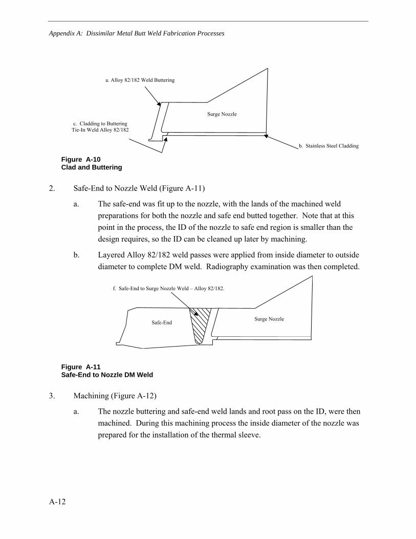
Appendix A: Dissimilar Metal Butt Weld Fabrication Processes

A-12

Figure A-10 Clad and Buttering

2. Safe-End to Nozzle Weld (Figure A-11)

a. The safe-end was fit up to the nozzle, with the lands of the machined weld preparations for both the nozzle and safe end butted together. Note that at this point in the process, the ID of the nozzle to safe end region is smaller than the design requires, so the ID can be cleaned up later by machining.

b. Layered Alloy 82/182 weld passes were applied from inside diameter to outside diameter to complete DM weld. Radiography examination was then completed.

Figure A-11 Safe-End to Nozzle DM Weld

3. Machining (Figure A-12)

a. The nozzle buttering and safe-end weld lands and root pass on the ID, were then machined. During this machining process the inside diameter of the nozzle was prepared for the installation of the thermal sleeve.

Surge Nozzle

a. Alloy 82/182 Weld Buttering

b. Stainless Steel Cladding

c. Cladding to Buttering Tie-In Weld Alloy 82/182

Surge Nozzle Safe-End

f. Safe-End to Surge Nozzle Weld – Alloy 82/182.

Appendix A: Dissimilar Metal Butt Weld Fabrication Processes

A-13

Figure A-12 Post DM Weld Machining

4. Thermal Sleeve Weld (Figure A-13)

a. The thermal sleeve is positioned and rolled into place. Following the rolling process an Alloy 82/182 weld, for 45 degrees of the circumference, is used to attach it to the safe end. Finally, the thermal sleeve attachment weld underwent PT exam.

Figure A-13 Thermal Sleeve Attachment Weld

A.3 Spray Nozzle Fabrication

The fabrication processes identified in Table A-1 apply to the spray nozzles. The details of these fabrication processes for the spray nozzles are similar to those provided in Section A.1 and A.2 for the surge nozzles; the “Back-Weld” process is best represented by Figure A-6 and Figure A-7 and the “Machined” process is best represented by Figure A-11 and Figure A-12.

The major difference in fabrication, besides nozzle bore diameter, is that a liner may be used in the place of cladding. Table A-4 provides additional information pertaining to spray nozzle fabrication.

• Plants D, F, and I spray nozzle bore is clad.

Surge Nozzle

Safe-End

h. Thermal Sleeve Attachment

Weld – Alloy 82/182

Thermal Sleeve

Safe-End

Surge Nozzle

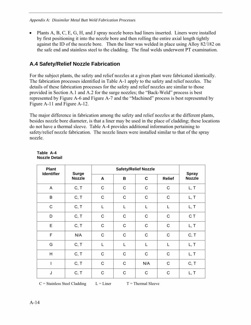
Appendix A: Dissimilar Metal Butt Weld Fabrication Processes

A-14

• Plants A, B, C, E, G, H, and J spray nozzle bores had liners inserted. Liners were installed by first positioning it into the nozzle bore and then rolling the entire axial length tightly against the ID of the nozzle bore. Then the liner was welded in place using Alloy 82/182 on the safe end and stainless steel to the cladding. The final welds underwent PT examination.

A.4 Safety/Relief Nozzle Fabrication

For the subject plants, the safety and relief nozzles at a given plant were fabricated identically. The fabrication processes identified in Table A-1 apply to the safety and relief nozzles. The details of these fabrication processes for the safety and relief nozzles are similar to those provided in Section A.1 and A.2 for the surge nozzles; the “Back-Weld” process is best represented by Figure A-6 and Figure A-7 and the “Machined” process is best represented by Figure A-11 and Figure A-12.

The major difference in fabrication among the safety and relief nozzles at the different plants, besides nozzle bore diameter, is that a liner may be used in the place of cladding; these locations do not have a thermal sleeve. Table A-4 provides additional information pertaining to safety/relief nozzle fabrication. The nozzle liners were installed similar to that of the spray nozzle.

Table A-4 Nozzle Detail

Safety/Relief Nozzle Plant Identifier Surge

Nozzle A B C Relief Spray Nozzle

A C, T C C C C L, T

B C, T C C C C L, T

C C, T L L L L L, T

D C, T C C C C C T

E C, T C C C C L, T

F N/A C C C C C, T

G C, T L L L L L, T

H C, T C C C C L, T

I C, T C C N/A C C, T

J C, T C C C C L, T

C = Stainless Steel Cladding L = Liner T = Thermal Sleeve

Appendix A: Dissimilar Metal Butt Weld Fabrication Processes

A-15

A.5 Design Sketches

Figures A-14 through A-38 are sketches of the nozzle designs covering each of the 51 subject welds. Figures A-14 through A-22 cover the 35 safety/relief nozzles, Figures A-23 through A-30 cover the 8 spray nozzles, and Figures A-31 through A-38 cover the 8 surge nozzles.

The figures provided in this appendix are not the final production manufacturing drawings. Manufacturing details were revealed later in the course of this project, and drawings showing the final manufactured state for each plant’s nozzles are not as readily available as the design drawings. In some cases, the manufacturing process used for a given plant (per Table A-1) differs from the one suggested by the design drawing. For example, comparing Figure A-14 (safety/relief Plant A) to Figure A-18 (safety/relief Plant E), it would be concluded the plants A and E share the same manufacturing process. However, as noted in Table A-1, plants A and E do not share the same process.

The plants affected by this difference between design and manufacturing are plants E and H. The design drawings for these plants are consistent with a “Back-Weld” process, but they were manufactured using a “Machined” process. The figures for these plants are still relevant, however. The “Machined” process did not change the final outline dimensions of the safe end, weld, or nozzle relative to the design drawings. Therefore, for example, the thickness of the weld for these plants are the same as indicated in the design drawings. In order to avoid confusion, a note is provided on the figures for plants E and H, referring to this section for additional information.

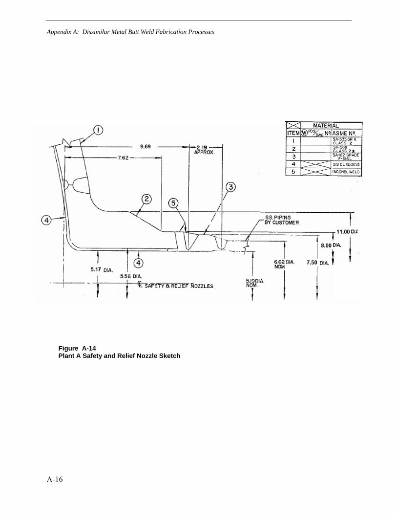
Appendix A: Dissimilar Metal Butt Weld Fabrication Processes

A-16

Figure A-14 Plant A Safety and Relief Nozzle Sketch

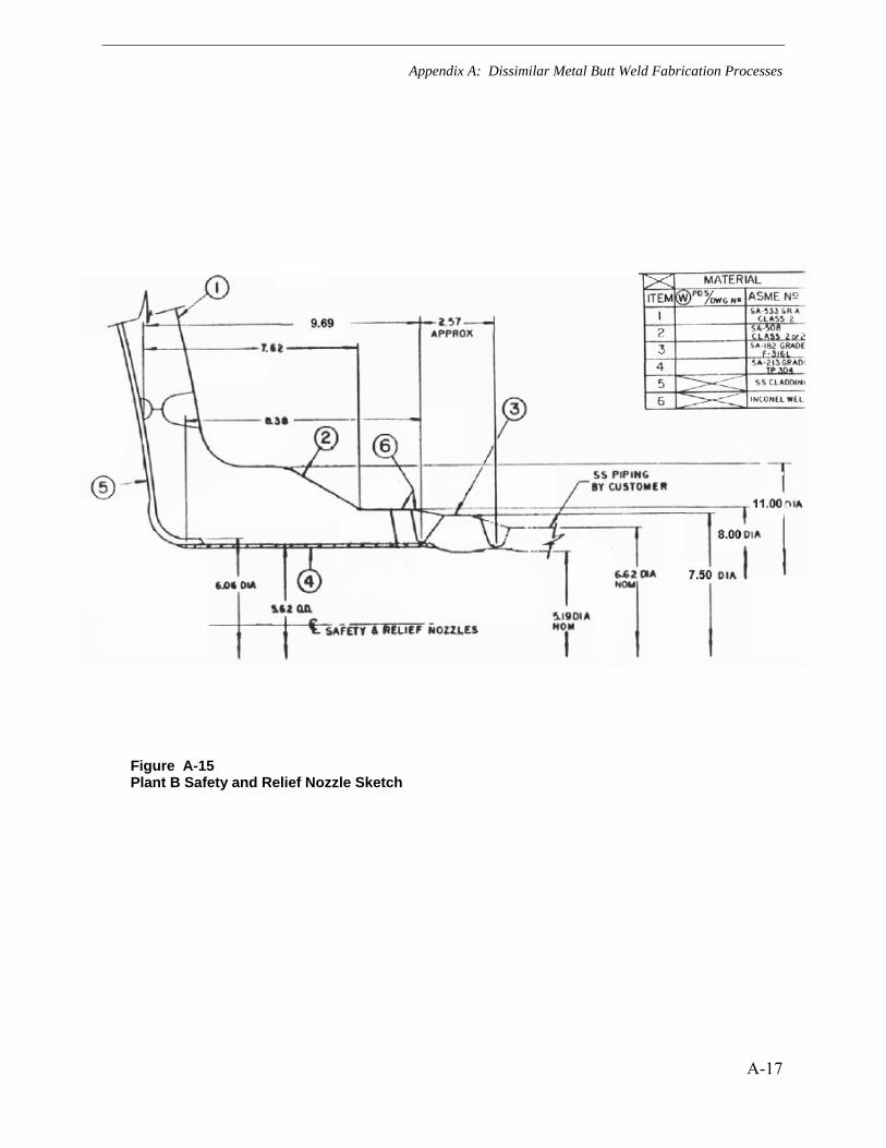
Appendix A: Dissimilar Metal Butt Weld Fabrication Processes

A-17

Figure A-15 Plant B Safety and Relief Nozzle Sketch

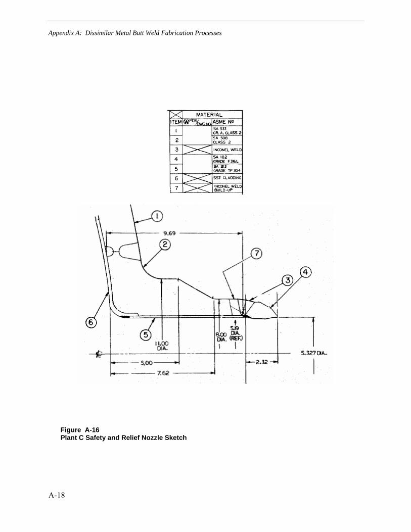
Appendix A: Dissimilar Metal Butt Weld Fabrication Processes

A-18

Figure A-16 Plant C Safety and Relief Nozzle Sketch

Appendix A: Dissimilar Metal Butt Weld Fabrication Processes

A-19

Figure A-17 Plant D Safety and Relief Nozzle Sketch

Appendix A: Dissimilar Metal Butt Weld Fabrication Processes

A-20

Figure A-18 Plant E Safety and Relief Nozzle Sketch

Note: The manufacturing process suggested by this drawing differs from the actual manufacturing process. The outline dimensions provided in this figure are not affected by the difference. See Section A.5 for additional details.

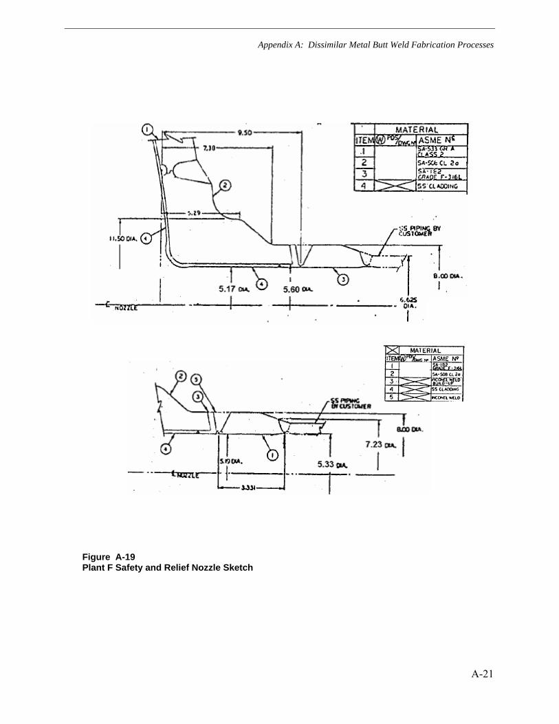
Appendix A: Dissimilar Metal Butt Weld Fabrication Processes

A-21

Figure A-19 Plant F Safety and Relief Nozzle Sketch

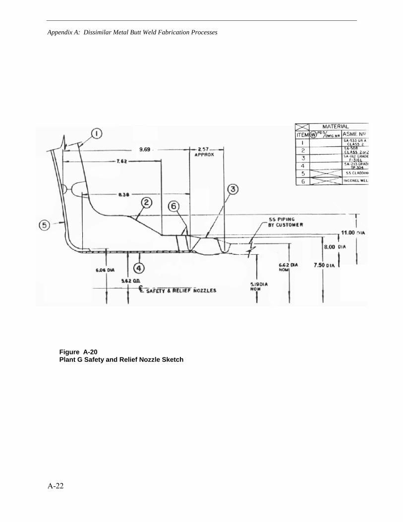
Appendix A: Dissimilar Metal Butt Weld Fabrication Processes

A-22

Figure A-20 Plant G Safety and Relief Nozzle Sketch

Appendix A: Dissimilar Metal Butt Weld Fabrication Processes

A-23

Figure A-21 Plant H Safety and Relief Nozzle Sketch

Note: The manufacturing process suggested by this drawing differs from the actual manufacturing process. The outline dimensions provided in this figure are not affected by the difference. See Section A.5 for additional details.

Appendix A: Dissimilar Metal Butt Weld Fabrication Processes

A-24

Figure A-22 Plant I Safety and Relief Nozzle Sketch

Appendix A: Dissimilar Metal Butt Weld Fabrication Processes

A-25

`

Figure A-23 Plant A Spray Nozzle Sketch

Appendix A: Dissimilar Metal Butt Weld Fabrication Processes

A-26

Figure A-24 Plant B Spray Nozzle Sketch

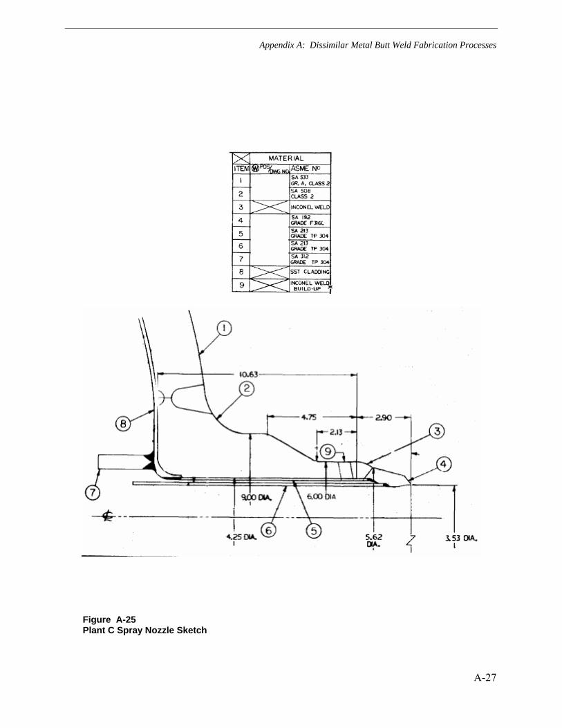
Appendix A: Dissimilar Metal Butt Weld Fabrication Processes

A-27

Figure A-25 Plant C Spray Nozzle Sketch

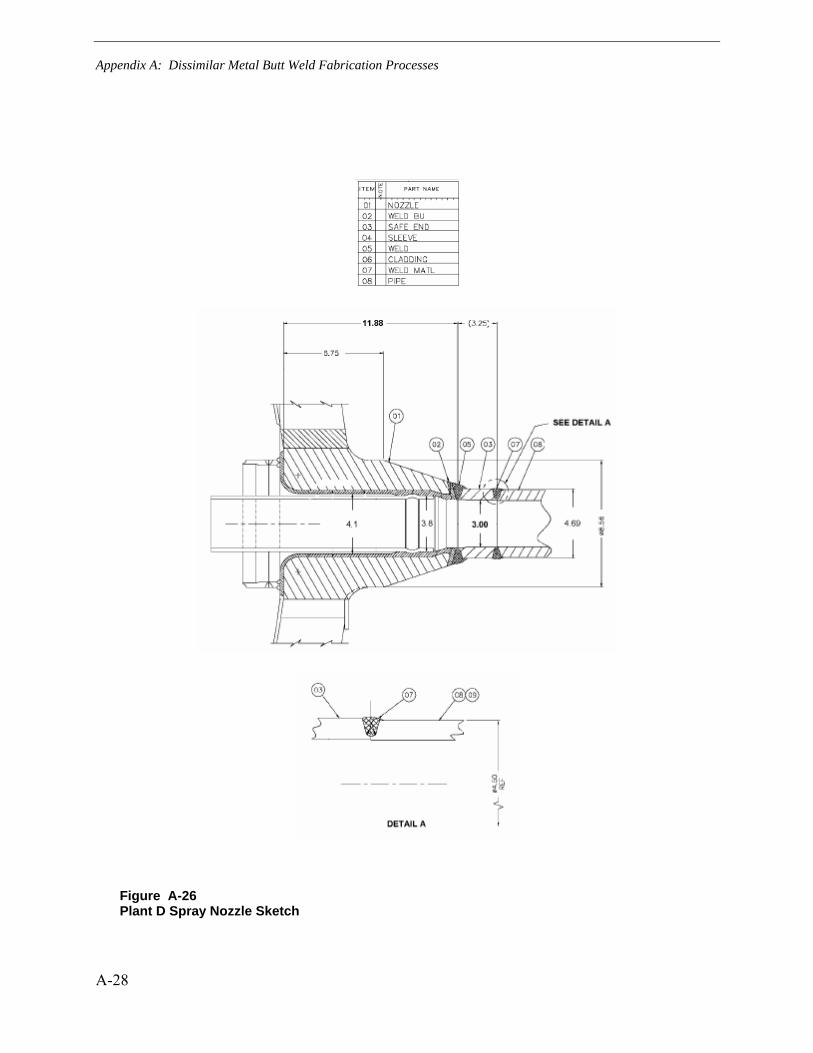
Appendix A: Dissimilar Metal Butt Weld Fabrication Processes

A-28

Figure A-26 Plant D Spray Nozzle Sketch

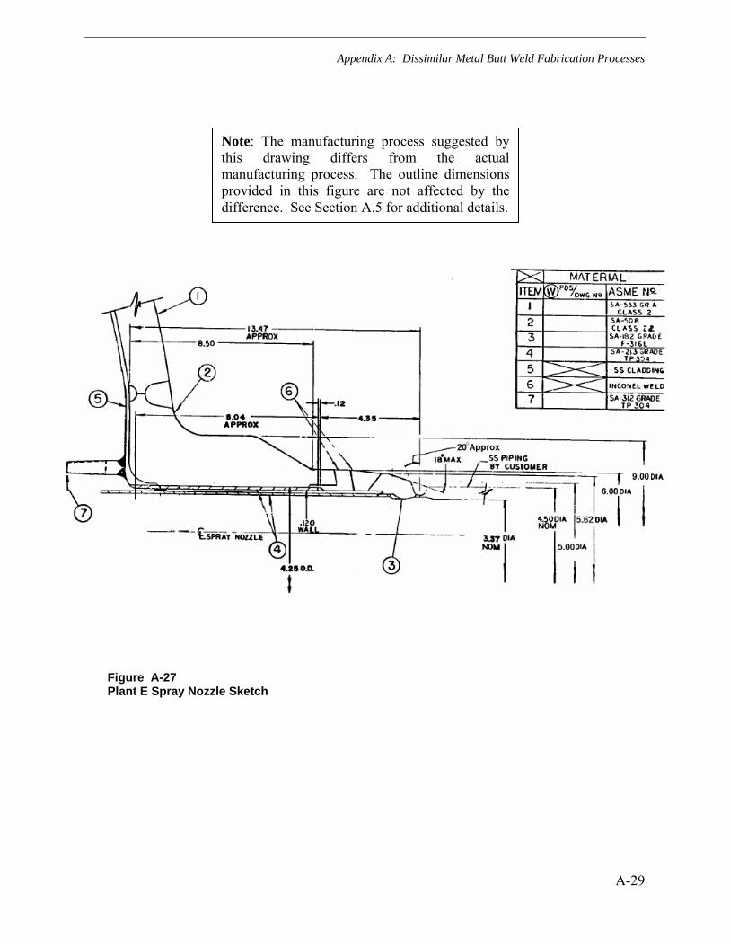
Appendix A: Dissimilar Metal Butt Weld Fabrication Processes

A-29

Figure A-27 Plant E Spray Nozzle Sketch

Note: The manufacturing process suggested by this drawing differs from the actual manufacturing process. The outline dimensions provided in this figure are not affected by the difference. See Section A.5 for additional details.

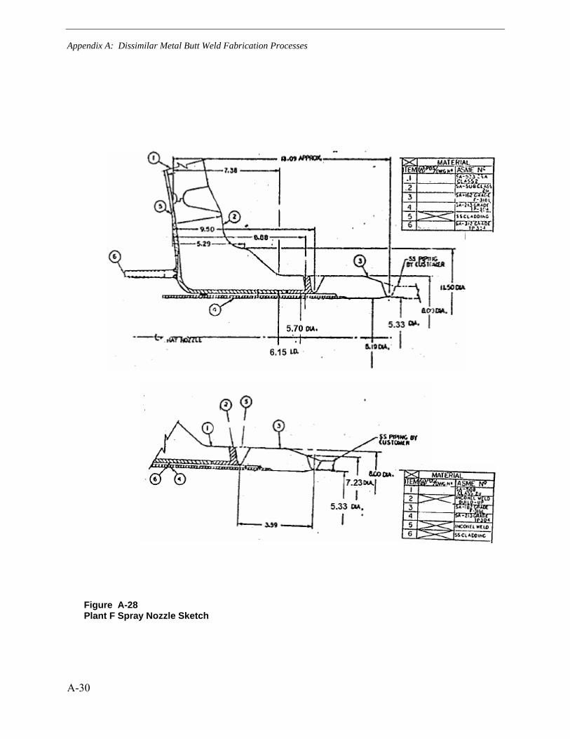
Appendix A: Dissimilar Metal Butt Weld Fabrication Processes

A-30

Figure A-28 Plant F Spray Nozzle Sketch

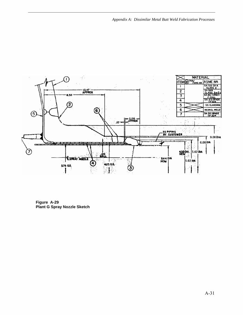
Appendix A: Dissimilar Metal Butt Weld Fabrication Processes

A-31

Figure A-29 Plant G Spray Nozzle Sketch

Appendix A: Dissimilar Metal Butt Weld Fabrication Processes

A-32

Figure A-30 Plant I Spray Nozzle Sketch

Appendix A: Dissimilar Metal Butt Weld Fabrication Processes

A-33

Figure A-31 Plant A Surge Nozzle Sketch

Appendix A: Dissimilar Metal Butt Weld Fabrication Processes

A-34

Figure A-32 Plant B Surge Nozzle Sketch

Appendix A: Dissimilar Metal Butt Weld Fabrication Processes

A-35

Figure A-33 Plant C Surge Nozzle Sketch

Appendix A: Dissimilar Metal Butt Weld Fabrication Processes

A-36

Figure A-34 Plant D Surge Nozzle Sketch

Appendix A: Dissimilar Metal Butt Weld Fabrication Processes

A-37

Figure A-35 Plant E Surge Nozzle Sketch

Note: The manufacturing process suggested by this drawing differs from the actual manufacturing process. The outline dimensions provided in this figure are not affected by the difference. See Section A.5 for additional details.

Appendix A: Dissimilar Metal Butt Weld Fabrication Processes

A-38

Figure A-36 Plant G Surge Nozzle Sketch

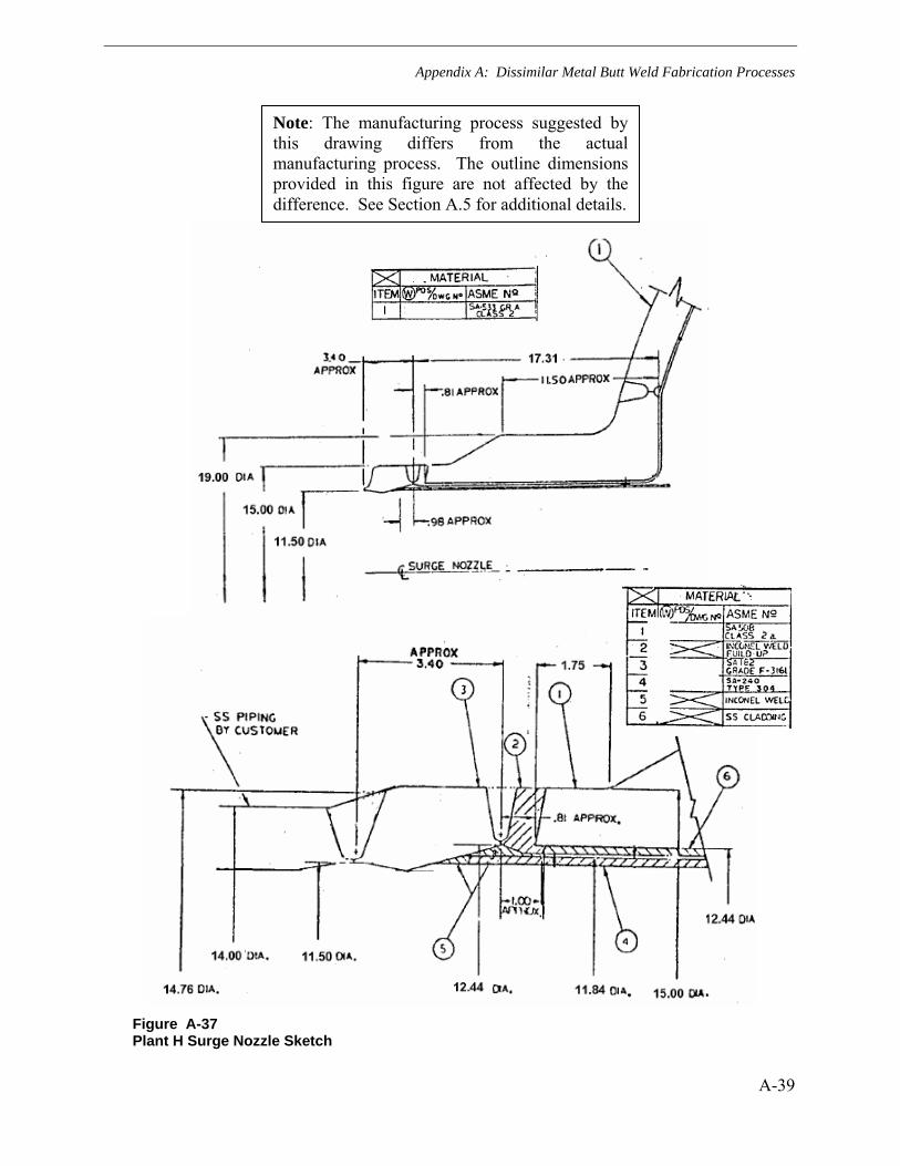
Appendix A: Dissimilar Metal Butt Weld Fabrication Processes

A-39

Figure A-37 Plant H Surge Nozzle Sketch

Note: The manufacturing process suggested by this drawing differs from the actual manufacturing process. The outline dimensions provided in this figure are not affected by the difference. See Section A.5 for additional details.

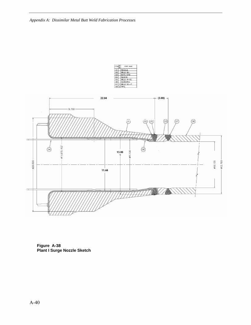
Appendix A: Dissimilar Metal Butt Weld Fabrication Processes

A-40

Figure A-38 Plant I Surge Nozzle Sketch

B-1

B APPENDIX B: EVALUATION OF THE EFFECTS OF SECONDARY STRESSES ON SURGE LINE CRITICAL FLAW SIZE CALCULATIONS

Appendix B was prepared by

Structural Integrity Associates, Inc. 6855 South Havana Street Suite 350 Centennial, CO 80112

Principal Investigators P. Riccardella P. Hirschberg

B.1 Introduction

In support of the critical flaw size analyses being performed in the main body of this report, analyses were performed to evaluate the effects of secondary (displacement controlled) loads on critical flaw size. The evaluation included a review of test data from the NRC-sponsored Degraded Piping Program [B-1,B-2]. Detailed test data from selected full scale pipe tests of relevant materials, pipe sizes and flaw types were reviewed to determine the amount of crack plane rotation that was tolerated in the tests prior to failure.

Piping models were also developed for the surge lines of two representative plants in the advanced FEA study (Plants C and I, Westinghouse and CE plant designs, respectively). The piping models were run under secondary operational loading conditions, including anchor movements, thermal expansion and worst case thermal stratification loads for these surge lines. The surge nozzle secondary stresses from these runs were observed to be at the high end of stresses for all nozzles in the study. Then, the models were re-run, after releasing all rotational degrees of freedom at the nodes representing the surge nozzles in the models. The resulting rotations at those nodes were determined, and compared to the rotational tolerance of flawed piping determined from the pipe test data. This comparison evaluates the maximum capacity of the secondary loads to produce rotation at a cracked surge nozzle, relative to the rotational tolerance of a nozzle weld containing a large complex crack.

Also, since the pipe tests did not include any tests of the nozzle weldment material (Alloy-182), a comparison of material toughness properties (J-R curves) of the pipe test materials to Alloy-182 was also performed.

Appendix B: Evaluation of the Effects of Secondary Stresses on Surge Line Critical Flaw Size Calculations

B-2

B.2 Full Scale Pipe Fracture Experiments

B.2.1 Test Data

Approximately 60 full scale pipe tests were conducted in the NRC-sponsored Degraded Piping Program [B-1,B-2] of pipes containing three types of circumferential defects: through-wall cracks, surface cracks, and complex cracks (see Figure B-1). Pipe sizes ranged from 4” to 42” and loadings included 4-point bending, combined bending + internal pressure and pure axial load. The majority of pipes tested were in the 6” to 16” range which is directly relevant to the current evaluation.

Selected test data from the Degraded Piping Program [B-1,B-2] are presented in Figures B-2 and B-3. Figure B-2 presents plots of crack plane rotation versus applied stress in the pipe for a series of 6-inch diameter stainless steel pipe tests containing the various crack types illustrated in Figure B-1 (complex cracks of two different sizes, thru-wall and surface cracks). Crack sizes are indicated in the plot legend in terms of lost cross sectional area caused by the crack (CF%). Figure B-3 shows similar plots, comparing crack plane rotation versus applied stress plots for tests with complex cracks only. This plot contains data from two different pipe sizes (6-inch and 16-inch), as well as two different complex flaw sizes (CFs = ~57% and 77%). Once again, all tests were austenitic stainless steel pipe.

In some of the tests reported in Figures B-2 and B-3, an inclinometer was used in the test to measure crack plane opening angle directly. In others, inclinometer data were not available, so the crack plane opening angle was computed from measured crack mouth opening displacement using the following formula:

COA = ArcTan (CMOD/pipe Diameter)

where,

COA = Crack Plane Opening Angle (degrees) CMOD = Measured crack mouth opening displacement (at maximum opening location on crack)

This method of estimating crack opening angle was checked against inclinometer measurements for the pipe tests in which both types of measurements were available, and found to be reasonable, but on the low or conservative side (Table B-1, last column).

B.2.2 Permissible Rotations

Review of the plots in Figures B-2 and B-3 illustrate that in all cases, the pipe tests were able to sustain significant rotations, on the order of 2° or greater, prior to maximum load. Beyond that point, the load decreased, with additional rotation tolerated, until ultimate fracture of the pipe at rotations of 7° or greater. (The curve for test 4114-3 in Figure B-3 appears to end at a smaller rotation, ~3.5°, but this corresponded to failure of the displacement gage, not the end of the test.)

Appendix B: Evaluation of the Effects of Secondary Stresses on Surge Line Critical Flaw Size Calculations

B-3

A summary of the various tests and the corresponding crack plane rotations at maximum load is given in Table B-1.

It is seen from this table that the only exception to the observation of rotations on the order of ~2° or greater, prior to maximum load, is the surface crack test, 4131-6, which had rotation of 1.67° at maximum load. This is not unexpected, as the surface crack geometry is not expected to be as compliant as the other crack geometries, and even this amount of rotation tolerance is not insignificant. Another observation regarding the surface crack test is that maximum load did not correspond to failure of the pipe, but rather to break-through of the surface crack to a through-wall crack, which, as illustrated by the plot for this test in Figure B-2, is still able to support significant loading and additional rotation as the test progressed beyond that point.

On the basis of these test results, it is concluded that all but the surface crack geometry can sustain crack plane rotations on the order of 2° or greater prior to failure of the pipe, considering relatively large flaws (CFs between 36% and 77%) and pipe sizes that are relevant to the current evaluation of pressurizer nozzles (6”and 16” nominal pipe diameters). For the surface flaw geometry, the rotational tolerance is slightly smaller, on the order of 1.67°. These observed crack plane rotations are conservatively assumed to be the permissible rotation for cracks of these sizes and configurations in austenitic piping materials. On the basis of the complete curves in Figures B-2 and B-3, crack plane rotations much greater than these values are expected to be tolerated, beyond maximum load, but prior to fracture. However, a more advanced analysis, considering relative compliance of the crack plane versus that of the piping system would be required to take advantage of this additional flaw tolerance, which is beyond the scope of the current study.

B.2.3 Material Toughness

Pipe materials used in the Degraded Piping Program full scale pipe tests included 304 stainless steel, A-600 and Carbon Steel base metals, but no weldments of direct relevance to the A-182 and A-82 dissimilar metal welds (DMWs) of interest in the current evaluation. Therefore the results of the base material pipe tests must be interpreted relative to pressurizer nozzle DMWs on the basis of relative material properties. Fortunately, the piping materials used in the tests were extensively characterized in terms of tensile properties and fracture toughness (J-R curves). Data also exists on the J-R properties of a large A-182 weldment and an A-82 weldment, which can be used for comparison to the test materials.

Figure B-4 presents a compilation of EPFM toughness data (J-R curves) from a number of sources [B-1 through B-5]. The pink dashed curves represent compact tension specimen J-R curves for a large A-182 weldment [B-3], and the sea green dashed curve is for an A-82 weldment [B-4]. These curves represent the weldment materials of interest in pressurizer DMWs. The solid curves are for austenitic base materials (stainless steel + A-600), including the specific materials used for the complex crack pipe tests (blue, red and orange curves). It is seen from these data that, except for the orange A-600 curve, the base materials are not significantly different than the A-82/182 weldments. In fact one of the complex crack pipe test materials (304SS A24C) falls right on top of the A-182 data for crack extension up to ~0.1” and the A-82

Appendix B: Evaluation of the Effects of Secondary Stresses on Surge Line Critical Flaw Size Calculations

B-4

curve is much higher. Based on this toughness comparison, it is not expected that A-182 would behave significantly different than the base metals used in full scale pipe tests.

Also shown for comparison are J-R curves for two materials that would be considered “low toughness”, a stainless steel submerged arc weld (SAW) and a carbon steel material from the pipe test program, indicated by the heavy brown and black curves in the figure. Note that these material J-R curves lie significantly below the previously discussed curves for austenitic base metal and A-82/182 weldments. These are indicative of how low the toughness of the A-82/182 weldments would have to be before one would be concerned about significantly reduced toughness in these weldments.

On the basis of these materials toughness comparisons, it is reasonably concluded that the rotational tolerances observed in the stainless steel pipe tests (Figures B-2 and B-3) are representative of what would be observed if similar tests were conducted with A-82/182 DMWs.

B.3 Surge Line Piping Analyses

B.3.1 Piping Models

To evaluate the potential pipe rotations that can result from the maximum secondary loads at typical surge nozzles, piping analytical models were created. Two models were developed: one for a CE plant and one for a Westinghouse plant. The details of the piping geometry, including routing, pipe support types and locations, fitting details, and operating conditions, were included. The geometry of the surge line is very similar between plants of a particular NSSS vendor, therefore these models are considered to be typical and representative.

The approach taken was to apply typical enveloping secondary loads to the piping, and determine the resulting stresses and moments at the pressurizer surge nozzle. Then, the rotational degrees of freedom at the nozzle were released, and the magnitude of rotation produced by these loads was determined.

The piping analysis was done using the program PIPESTRESS [B-6]. PIPESTRESS is a fully verified computer code that implements the requirements of the ASME Section III piping design Code.

Figures B-5 and B-6 show the piping models.

B.3.2 Loading Cases

The secondary loadings that are applied to the surge line are three types:

Thermal expansion Anchor movements Thermal stratification

Appendix B: Evaluation of the Effects of Secondary Stresses on Surge Line Critical Flaw Size Calculations

B-5

For the CE plant, thermal expansion was based on a maximum pipe temperature of 653°F, corresponding to the pressurizer steam space temperature, which is conservative. Thermal anchor movements were applied at the hot leg and at the pressurizer nozzle. These were obtained from the Design Specification. For thermal stratification, a maximum top to bottom temperature gradient of 320°F was applied. This gradient was used in the CEOG generic stratification report.

For the Westinghouse plant, a similar approach was taken, except that thermal expansion was based on a temperature of 608°F, corresponding to the hot leg temperature, as is typical of Westinghouse analyses. The stratification gradient was 270°F, which is the maximum gradient in the Design Specification of the plant being analyzed.

B.3.3 Analysis Results

Table B-2 summarizes the results of the two analyses. The maximum secondary stress on the CE plant surge nozzle is 19.5 ksi, and in the Westinghouse plant is 24.9 ksi. When the rotational degrees of freedom are released at the nozzle, the rotation produced by the secondary loads is 1.81 degrees for the CE plant model, and 1.77 degrees for the Westinghouse plant model.

Thus, it is concluded that the rotation that would be produced by the maximum secondary loading on typical CE and Westinghouse surge lines does not exceed 2 degrees.

B.4 Conclusions

This evaluation was performed to determine the potential effects of secondary (displacement-controlled) stresses in surge line piping of plants in the advanced FEA project.

Full scale pipe test data from the Degraded Piping Program show that pipes containing large complex cracks can sustain greater than ~2° rotation at the crack plane prior to maximum loads being achieved in the tests. The permissible rotational tolerance would be even greater if additional rotation, beyond maximum load in the tests but prior to fracture, were credited.

The maximum rotation at the surge nozzle that could be produced by worst case secondary loads (anchor movement + thermal expansion + stratification) was demonstrated to be less than 2° for two representative surge lines in the advanced FEA project (one Westinghouse and one CE plant design). This was determined based on piping models of the two surge lines that included the applicable supports and system geometries.

Therefore, the secondary loads would be completely relieved prior to fracture of the nozzles, and critical flaw size calculations need only consider primary, load-controlled stresses.

Appendix B: Evaluation of the Effects of Secondary Stresses on Surge Line Critical Flaw Size Calculations

B-6

B.5 References

B-1. Summary of Technical Results and Their Significance to Leak-Before-Break and In-Service Flaw Acceptance Criteria, NUREG/CR-4082, Volume 8, March 1984 - January 1989.

B-2. Pipe Fracture Encyclopedia, U.S. NRC, 1997 (A collection of NUREG Reports and Data Files from the DP2 and other programs distributed on CDs).

B-3. G. Wilkowski, H. Xu, D.-J. Shim, and D. Rudland, “Determination of the Elastic-Plastic Fracture Mechanics Z-factor for Alloy 82/182 Weld Metal Flaws for Use in the ASME Section XI Appendix C Flaw Evaluation Procedures,” PVP2007-26733, Proceedings of ASME-PVP 2007: 2007 ASME Pressure Vessels and Piping Division Conference, San Antonio, TX, 2007.

B-4. W. J. Mills and C. M. Brown, “Fracture Toughness of Alloy 600 and EN82H Weld in Air and Water,” B-T-3264, Bettis Atomic Power Laboratory.

B-5. Toughness of Austenitic Stainless Steel Pipe Welds, EPRI, Palo Alto, CA: 1988. NP-4768.

B-6. Program PIPESTRESS, Version 3.5.1+026, DST Systems, June 2004.

Appendix B: Evaluation of the Effects of Secondary Stresses on Surge Line Critical Flaw Size Calculations

B-7

Table B-1 Summary of Crack Plane Rotations at Maximum Load in Pipe Tests

Crack Face Rotation at Max. Load (°)

Test Nominal Pipe Diam. (in.)

Crack Type

CF%

from CMOD Inclinometer

4113-1 6 Complex 56.6% 3.13

4113-2 6 Complex 76.7% 1.97

4131-5 6 Thru-Wall 38.9% 9.26

4131-6 6 Surface 36.9% 1.67

4114-3 16 Complex 58.5% 2.32 3.54

4114-4 16 Complex 58.5% 2.54 2.95

Table B-2 Piping Analysis Results

Summary of Results - Pressurizer Surge Nozzle Moment vs. RotationNotes

Mx, ft-kip My Mz Stress, ksi Rx, deg. Ry Rz SRSSCE Plant 176.303 43.701 5.771 19.485 1.38 0.66 0.97 1.81 1, 2, 3Westinghouse Plant 138.881 103.841 3.809 24.854 1.13 1.08 0.84 1.77 1, 2, 4

Notes:1. My is torsion direction. 2. Loads include thermal expnasion, anchor movement, and stratification3. Stratification delta T is 320 F.4. Stratification delta T is 270 F.

Fixed-Fixed Bending Moments Fixed-Pinned Rotations (Deg.)

Appendix B: Evaluation of the Effects of Secondary Stresses on Surge Line Critical Flaw Size Calculations

B-8

Figure B-1 Illustration of Circumferential Flaw Types Tested

Crack Rotation Comparison(All Pipes 6" NPS; Different Crack Types)

0.0

5.0

10.0

15.0

20.0

25.0

30.0

35.0

40.0

0.00 5.00 10.00 15.00

Rotation due to Crack (Deg.)

App

lied

Stre

ss (

Pb; k

si) 4113-1 Complex; CF= 56.6%

4113-2 Complex; CF=76.7%

4131-5 Thru; CF=38.9%

4131-6 Surface; CF=36.9%

Figure B-2 Plots of Crack Plane Rotation versus Applied Stress in Pipe Tests for Various Flaw Types – All Tests Austenitic Stainless Steel and 6-inch Nominal Pipe Size

Appendix B: Evaluation of the Effects of Secondary Stresses on Surge Line Critical Flaw Size Calculations

B-9

Crack Rotation Comparison(All Complex Cracks; Different Pipe Sizes)

0.0

2.0

4.0

6.0

8.0

10.0

12.0

14.0

16.0

18.0

0.00 5.00 10.00 15.00

Rotation due to Crack (Deg.)

App

lied

Stre

ss (

Pb; k

si)

4113-1 NPS-6; CF= 56.6%

4113-2 NPS-6; CF=76.7%

4114-3 NPS-16; CF=58.5%

4114-4; NPS-16; CF=58.5%

Figure B-3 Plots of Crack Plane Rotation versus Applied Stress in Pipe Tests for Various Pipe Sizes – All Tests Austenitic Stainless Steel and Complex Crack Geometry

0

2000

4000

6000

8000

10000

12000

14000

0.000 0.050 0.100 0.150 0.200 0.250 0.300 0.350 0.400 0.450 0.500

Crack Extension (in)

J (in

-lb/in

^2)

A-182 (BT-4;600F)A-182 (BT-3;600F)A-182 (WT-4;600F)A-182 (BR-1;600F)A-82 (Mills 640F)A-600 (Mills 640F)A-600 (Mills 640F)A-600 (I1C; 550F)304SS (Landes;550F)304SS (Landes;550F)316SS (Landes;550F)304SS (A24C; 550F)304SS (A8; 550F)304 SAW (Landes;550F)CS DP2-F30C

Figure B-4 Comparison of J-R Curves for All0y-182 to Various Pipe Test Materials. Two “Low Toughness” Materials also Plotted for Comparison

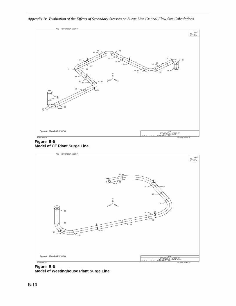
Appendix B: Evaluation of the Effects of Secondary Stresses on Surge Line Critical Flaw Size Calculations

B-10

07/26/07 10:50:07w3srg1test.fre

PSG-I 3.2 OCT 2004 (DOS)P

VSUP

10

2021

2223

303132

33

34

35

404142

43

44

5051

52

5354

60

6162

6364

7071

7280

EPRIST RUCTURAL I NT EGRI TY

CE S URGE LI NES CAL E: 1/ 48 E NGI NEER: PH

Figure A: STANDARD VIEW

Figure B-5 Model of CE Plant Surge Line

07/26/07 10:49:42dcpp2test.fre

PSG-I 3.2 OCT 2004 (DOS)P

VSUP

1015

20

21 23

25

30

31

32

34

35

4041

42

50

80

EPRIST RUCTURAL I NT EGRI TY

WES TI NGHOUSE SURGE LI NES CAL E: 1/ 48 E NGI NEER: PH

Figure A: STANDARD VIEW

Figure B-6 Model of Westinghouse Plant Surge Line

C-1

C APPENDIX C: SECONDARY STRESS STUDY—PIPE BENDING WITH A THROUGH-THICKNESS CRACK

Appendix C was prepared by

Quest Reliability, LLC 2465 Central Avenue Suite 110 Boulder, CO 80301

Principal Investigators T. Anderson G. Thorwald E. Scheibler

C.1 Introduction

Finite element analysis (FEA) of a pipe with a through-thickness crack was used to determine the effect on bending moment and crack driving force due to an imposed end rotation. The imposed end rotation bends the pipe and causes the through-thickness crack to open. An end rotation could be caused in a piping system by transverse pipe segments extending due to thermal expansion. The moment knock-down factors and crack driving force are computed for a range of crack lengths.

C.2 Analysis

The FEA pipe crack meshes were generated using the FEACrack software (Quest Reliability commercial software), and the analysis was run using ABAQUS (ABAQUS, Inc. software). Two pipe lengths were examined in the analysis. The total length, 2L, of the pipe models were: 60 in and 60 ft. The FEA models are quarter symmetric with a model length of L. The pipes have an inside radius, Rin of 6.0 in, and a thickness of 1.5 in. The initial bending stress in the pipe is 25 ksi (uncracked pipe).

The moment knock-down factor for a fixed rotation was computed for each crack length to evaluate the effect of the increasing crack length on the pipe bending moment. The moment knock-down factor is the ratio of the bending moment in the pipe with a crack, M, to the initial uncracked pipe bending moment, M0.

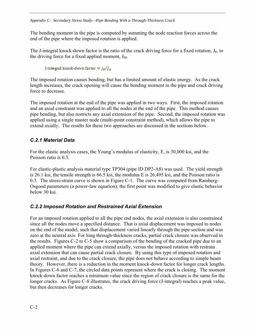
Appendix C: Secondary Stress Study—Pipe Bending With a Through-Thickness Crack

C-2

The bending moment in the pipe is computed by summing the node reaction forces across the end of the pipe where the imposed rotation is applied.

The J-integral knock-down factor is the ratio of the crack driving force for a fixed rotation, Jθ, to the driving force for a fixed applied moment, JM.

The imposed rotation causes bending, but has a limited amount of elastic energy. As the crack length increases, the crack opening will cause the bending moment in the pipe and crack driving force to decrease.

The imposed rotation at the end of the pipe was applied in two ways. First, the imposed rotation and an axial constraint was applied to all the nodes at the end of the pipe. This method causes pipe bending, but also restricts any axial extension of the pipe. Second, the imposed rotation was applied using a single master node (multi-point constraint method), which allows the pipe to extend axially. The results for these two approaches are discussed in the sections below.

C.2.1 Material Data

For the elastic analysis cases, the Young’s modulus of elasticity, E, is 30,000 ksi, and the Poisson ratio is 0.3.

For elastic-plastic analysis material type TP304 (pipe ID DP2-A8) was used. The yield strength is 26.1 ksi, the tensile strength is 66.5 ksi, the modulus E is 26,495 ksi, and the Poisson ratio is 0.3. The stress-strain curve is shown in Figure C-1. The curve was computed from Ramberg-Osgood parameters (a power-law equation); the first point was modified to give elastic behavior below 30 ksi.

C.2.2 Imposed Rotation and Restrained Axial Extension

For an imposed rotation applied to all the pipe end nodes, the axial extension is also constrained since all the nodes move a specified distance. That is axial displacement was imposed to nodes on the end of the model, such that displacement varied linearly through the pipe section and was zero at the neutral axis For long through-thickness cracks, partial crack closure was observed in the results. Figures C-2 to C-5 show a comparison of the bending of the cracked pipe due to an applied moment where the pipe can extend axially, versus the imposed rotation with restrain axial extension that can cause partial crack closure. By using this type of imposed rotation and axial restraint, and due to the crack closure, the pipe does not behave according to simple beam theory. However, there is a reduction in the moment knock-down factor for longer crack lengths. In Figures C-6 and C-7, the circled data points represent where the crack is closing. The moment knock-down factor reaches a minimum value since the region of crack closure is the same for the longer cracks. As Figure C-8 illustrates, the crack driving force (J-integral) reaches a peak value, but then decreases for longer cracks.

Appendix C: Secondary Stress Study—Pipe Bending With a Through-Thickness Crack

C-3

C.2.3 Imposed Rotation and Unrestrained Axial Extension

In the multi-point constraint (MPC) method, a single master node at the center of the pipe is grouped with the pipe end nodes, and the imposed rotation is applied to the master node. This method allows the axial extension of the pipe to remain unrestrained so that the pipe can extend while bending. Figures C-9 and C-10 show that since the pipe length is allowed to extend axially, the knock-down factors and crack driving force decrease to zero as the through-thickness crack length extends around the full pipe circumference. Comparing the crack driving force to an applied moment and applied rotation (Figures C-11 and C-12) shows that the bending moment applied unlimited strain to the pipe and the crack driving force is unbounded. The imposed rotation applies finite strain to the pipe and the crack driving force decreases after reaching a peak value. Figure C-13 shows that the J knock-down factor decreases with crack length.

C.3 Summary

The moment knock-down factor and crack driving force in a pipe with a through-thickness crack was examined by finite element analyses of quarter-symmetric pipe models; the pipe models have two lengths (short and long) and a range of crack lengths. An imposed rotation was applied at the end of the pipe to cause the pipe bending. Elastic and elastic-plastic analysis results were compared. The finite amount of strain imposed by the rotation shows that the moment knock-down factor and crack driving force relative to the load controlled case decrease significantly as the crack length increases.

The results of this calculation demonstrate that a circumferential crack in a cylinder responds differently to bending generated by a displacement-controlled source (rotation) versus one generated by a load-controlled source (moment). Even with bending applied to a 60-foot length of piping, the applied moment under displacement loading was found to reduce greatly as the crack length increased. Figures C-10 and C-13 show the key results, which demonstrate the general tendency for relief of secondary piping loads given sufficient crack plane rotation.

Appendix C: Secondary Stress Study—Pipe Bending With a Through-Thickness Crack

C-4

0

10

20

30

40

50

60

70

80

90

0 0.1 0.2 0.3 0.4 0.5 0.6 0.7

True Plastic Strain

True

Stre

ss, k

si

Ramberg-Osgood

Assumed for FEA

Figure C-1 Stress-Strain Curve for Elastic-Plastic Analysis

Figure C-2 Schematic of Pipe Bending due to an Applied Moment

Appendix C: Secondary Stress Study—Pipe Bending With a Through-Thickness Crack

C-5

Figure C-3 Schematic of Pipe Bending due to an Imposed Rotation and Restrained Axial Extension

Figure C-4 Elastic FEA Results, Imposed Rotation and Axial Restraint; Crack Closure

Appendix C: Secondary Stress Study—Pipe Bending With a Through-Thickness Crack

C-6

Figure C-5 Elastic FEA Results, Imposed Moment

Figure C-6 Elastic Analysis, Moment Knock-Down Factors

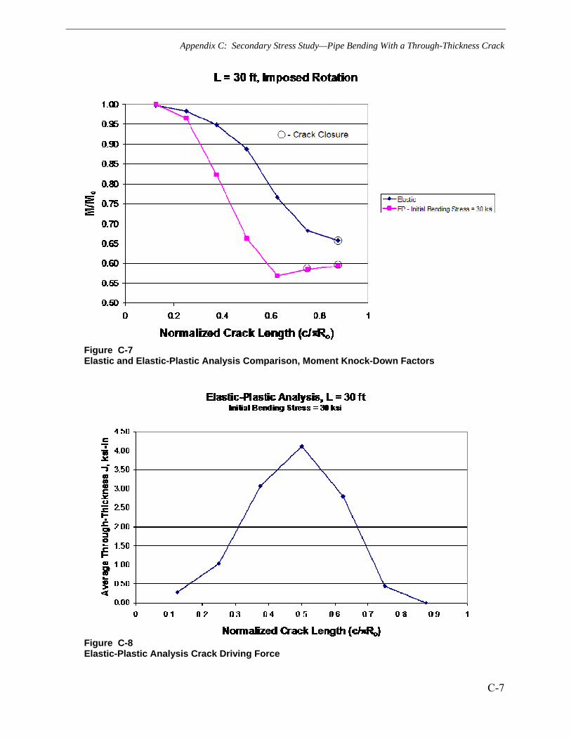
Appendix C: Secondary Stress Study—Pipe Bending With a Through-Thickness Crack

C-7

Figure C-7 Elastic and Elastic-Plastic Analysis Comparison, Moment Knock-Down Factors

Figure C-8 Elastic-Plastic Analysis Crack Driving Force

Appendix C: Secondary Stress Study—Pipe Bending With a Through-Thickness Crack

C-8

Figure C-9 Moment Knock-Down Factors, Elastic Analysis, MPC Imposed Rotation Only

Figure C-10 Moment Knock-Down Factors, Elastic-Plastic Analysis, MPC Imposed Rotation Only

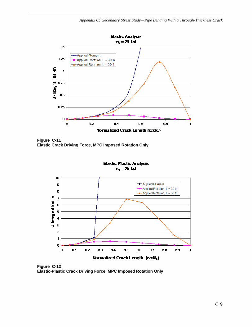
Appendix C: Secondary Stress Study—Pipe Bending With a Through-Thickness Crack

C-9

Figure C-11 Elastic Crack Driving Force, MPC Imposed Rotation Only

Figure C-12 Elastic-Plastic Crack Driving Force, MPC Imposed Rotation Only

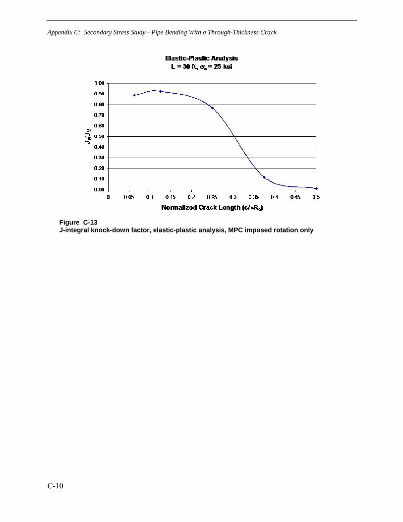
Appendix C: Secondary Stress Study—Pipe Bending With a Through-Thickness Crack

C-10

Figure C-13 J-integral knock-down factor, elastic-plastic analysis, MPC imposed rotation only

D-1

D APPENDIX D: SCATTER IN LEAK RATE PREDICTIONS

Appendix D was prepared by

Structural Integrity Associates, Inc. 6855 South Havana Street Suite 350 Centennial, CO 80112

Principal Investigator D. Harris

D.1 Evaluation

The purpose of this note is to summarize the results of a study performed regarding accuracy of leak rate predictions from cracks in pipes. This study was requested at the meeting on June 19 and 20 at Dominion Engineering offices in Reston, Virginia. A word document of Reference D-1 was provided in an e-mail from David Rudland of EMC2 on June 22. IGSCC crack leak rate data from Table B.5 of this reference was employed. This provides about 82 data points of predicted leak rate versus measured leak rate. Table D-1 summarizes the data for which both measured and predicted values are available. This table is in gallons per minute (gpm), which have been converted from the kg/sec used in Reference D-1. Figure D-1 is a plot of this data.

Note that the scatter in the data is much larger at low leak rates, say below 0.1 gpm. This is consistent with the figure shown in the meeting at Dominion Engineering.

The leak rate data was sorted to include only measured leak rates above 0.1 gpm, since small leak rates are not of interest in this context. Values of the ratio of the measured to the predicted leak rates were calculated for the pruned data, which was then sorted in ascending order of this ratio. Table D-2 lists the 34 resulting points. The probability was evaluated from the formula P=(I-½)/N. Figure D-2 presents a normal and lognormal plot of the data.

Figure D-2 shows that the data is not well fit by either a normal or lognormal distribution, and that the 95th percentile is about 1.5. This means that there is a 95% probability that the actual (measured) leak rate will not exceed the calculated value by more than a factor of 1.5.

Another reading on the scatter in leak rate predictions can be obtained from results from Reference D-2, which provides the following relation for the standard deviation of the leak rate for a given mean:

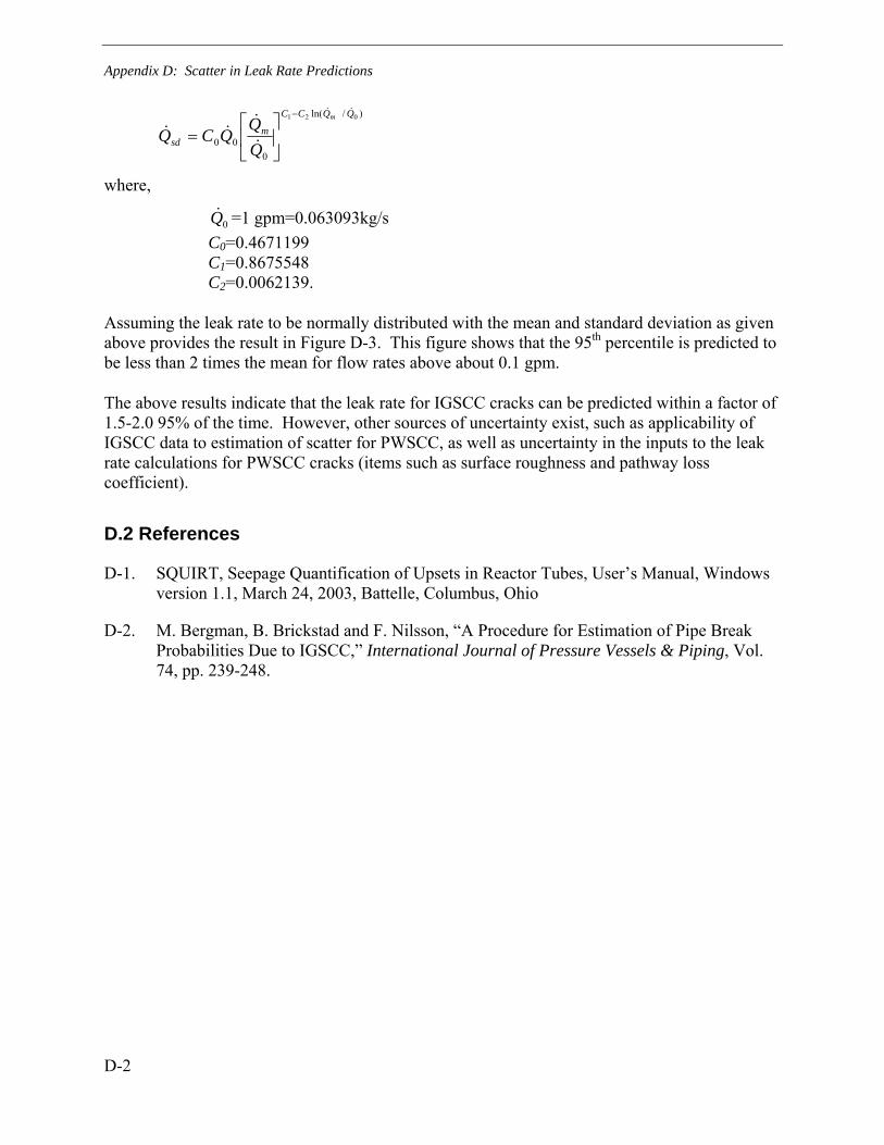
Appendix D: Scatter in Leak Rate Predictions

D-2

)/ln(

000

021 QQCC

msd

m

QQ

QCQ−

⎥⎦

⎤⎢⎣

⎡=

where,

0Q =1 gpm=0.063093kg/s C0=0.4671199 C1=0.8675548 C2=0.0062139.

Assuming the leak rate to be normally distributed with the mean and standard deviation as given above provides the result in Figure D-3. This figure shows that the 95th percentile is predicted to be less than 2 times the mean for flow rates above about 0.1 gpm.

The above results indicate that the leak rate for IGSCC cracks can be predicted within a factor of 1.5-2.0 95% of the time. However, other sources of uncertainty exist, such as applicability of IGSCC data to estimation of scatter for PWSCC, as well as uncertainty in the inputs to the leak rate calculations for PWSCC cracks (items such as surface roughness and pathway loss coefficient).

D.2 References

D-1. SQUIRT, Seepage Quantification of Upsets in Reactor Tubes, User’s Manual, Windows version 1.1, March 24, 2003, Battelle, Columbus, Ohio

D-2. M. Bergman, B. Brickstad and F. Nilsson, “A Procedure for Estimation of Pipe Break Probabilities Due to IGSCC,” International Journal of Pressure Vessels & Piping, Vol. 74, pp. 239-248.

Appendix D: Scatter in Leak Rate Predictions

D-3

Table D-1 Listing of IGSCC Data from Table B.5 of Reference 1 (Leak Rates in gpm)

Measured Predicted Measured Predicted

0.016 0.094 0.029 0.021 0.016 0.094 0.031 0.027 0.017 0.121 0.035 0.031 0.017 0.138 0.038 0.034 0.017 0.138 0.006 0.021 0.017 0.13 0.008 0.029 0.001 0.003 0.062 0.031 0.001 0.004 0.069 0.034

0 0.001 0.051 0.022 0 0.002 0.057 0.029

0.002 0.002 0.04 0.014 0.002 0.002 0.056 0.026 0.002 0.002 0.065 0.032 0.001 0.001 0.035 0.015 0.002 0.001 0.041 0.025 0.002 0.001 0.05 0.032 0.482 0.403 0.012 0.009 0.46 0.323 0.014 0.02

0.769 0.501 0.024 0.026 0.732 0.537 0.029 0.031 0.716 0.618 0.028 0.026 0.704 0.612 0.024 0.02 0.582 0.488 0.021 0.013 0.569 0.485 0.029 0.009 0.398 0.314 0.037 0.02 0.372 0.263 0.043 0.026 0.477 0.425 0.043 0.031 0.472 0.415 2.393 5.468 0.628 0.556 2.488 4.406 0.624 0.575 2.774 5.405 0.715 0.667 2.235 1.759 0.75 0.689 2.679 4.01

0.609 0.613 3.027 5.341 0.621 0.623 3.17 5.373 0.609 0.521 2.821 4.184 0.471 0.496 2.393 1.965 0.415 0.311 2.029 1.062 0.249 0.301 2.79 4.359

3.154 5.405

Appendix D: Scatter in Leak Rate Predictions

D-4

Table D-2 Ratio of Measured to Predicted Leak Rates for IGSCC Data from Table B.5 of Reference 1 with Measured Leak Rate Greater than 0.1 gpm

ratio probability ratio probability

0.438 0.0147 1.128 0.5147 0.513 0.0441 1.137 0.5441 0.565 0.0735 1.15 0.5735 0.567 0.1029 1.159 0.6029 0.584 0.1324 1.167 0.6324 0.59 0.1618 1.173 0.6618 0.64 0.1912 1.192 0.6912

0.668 0.2206 1.197 0.7206 0.674 0.25 1.218 0.75 0.826 0.2794 1.268 0.7794 0.949 0.3088 1.27 0.8088 0.992 0.3382 1.337 0.8382 0.998 0.3676 1.363 0.8676 1.071 0.3971 1.416 0.8971 1.085 0.4265 1.422 0.9265 1.087 0.4559 1.535 0.9559 1.123 0.4853 1.91 0.9853

10-3

10-2

0.1

1

10

10-3 10-2 0.1 1 10

measured leak rate, gpm

pred

icte

d le

ak ra

te, g

pm

leak rate comparisonD:\FortranStuff\SQIRT.OUT

Figure D-1 Predicted Leak Rate versus Measured Leak Rate for IGSCC Data

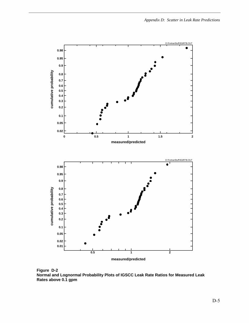
Appendix D: Scatter in Leak Rate Predictions

D-5

0.02

0.05

0.1

0.2

0.3

0.40.50.6

0.7

0.8

0.9

0.95

0.98

0 0.5 1 1.5 2

measured/predicted

cum

ulat

ive

prob

abili

ty

D:\FortranStuff\SQIRTB.OUT

0.010.02

0.05

0.1

0.2

0.30.40.50.60.7

0.8

0.9

0.95

0.98

0.5 1 2

measured/predicted

cum

ulat

ive

prob

abili

ty

D:\FortranStuff\SQIRTB.OUT

Figure D-2 Normal and Lognormal Probability Plots of IGSCC Leak Rate Ratios for Measured Leak Rates above 0.1 gpm

Appendix D: Scatter in Leak Rate Predictions

D-6

0

1

2

3

0 2 4 6 8 10

calculated flow rate, gpm

Q95

/Qm

D:\FortranStuff\QDOT.OUT

Figure D-3 Ratio of the 95th Percentile to the 50th Percentile of Flow Rate as a Function of the (Mean) Calculated Flow Rate

E-1

E APPENDIX E: EVALUATION OF PRESSURIZER ALLOY 82/182 NOZZLE FAILURE PROBABILITY

Appendix E was prepared by

Structural Integrity Associates, Inc. 6855 South Havana Street Suite 350 Centennial, CO 80112

Principal Investigators P. Riccardella D. Dedhia D. Harris

E.1 Introduction

To complement the deterministic analyses described in the main body of this report, the MRP also performed a probabilistic evaluation of the Alloy 82/182 pressurizer butt welded nozzles, considering current inspection data, to assess the effect of various inspection options on the probability of a nozzle failure in the time interval until all nozzles are inspected or mitigated. There are three major elements to the probabilistic analysis approach:

1. FLAW DISTRIBUTION. As discussed in Section E.2 of this report, considering inspections performed through Spring of 2007, data exists for a total of 50 Alloy 82/182 nozzles that either have been inspected as part of the MRP-139 inspection program [E-1], or in which leaks, cracks or UT indications have been detected prior to the commencement of MRP-139 examinations in 2006. These data, summarized in Table E-1, and illustrated graphically in Figure E-2, are used to estimate probable flaw distributions that might exist in uninspected nozzles.

2. FRAGILITY CURVE. A second important aspect of the analysis, discussed in Section E.3, is the critical flaw size to cause a nozzle failure. For any given flaw size, characterized in terms of percentage of cross section lost to the crack (denoted in this report as the Criticality Factor, CF%), there is a probability that the flaw will cause a pipe rupture under operating loads and internal pressure. This probability of rupture versus flaw size is called a “fragility curve” which can be combined with a probable flaw distribution to estimate the cumulative probability of a nozzle failure in the time period up to the time of the recent inspections.

Appendix E: Evaluation of Pressurizer Alloy 82/182 Nozzle Failure Probability

E-2

3. CRACK GROWTH. The flaw distribution discussed in 1 above represents a snapshot at the time of the inspections. In order to make meaningful comparisons of future probabilities of rupture under various inspection scenarios, estimates of the probability of future flaw growth must be made. The deterministic results of Section 7 of the main body of this report are used, as discussed in Section E.4, to produce a series of flaw distributions similar to those discussed in 1 above, but which increase with time. These time-varying crack size distributions are used in conjunction with the fragility curve to produce estimates of the probability of rupture versus time into the future (at six month intervals).

The analysis process is illustrated in Figure E-1. A typical flaw distribution (Weibull) at the time of the recent inspections is illustrated by the curve on the left hand side of the graph. This curve is estimated to shift to the right due to crack growth during each six-month period between outage seasons, as illustrated by the series of parallel dashed curves in the figure. Finally, the fragility curve is illustrated by the red curve on the right hand side of the figure. Figure E-1b is a zoom-in view of the low probability region of the same graph.

The failure probability is actually simulated by a process of Monte Carlo sampling from a flaw distribution and the fragility curve, as discussed in detail in Section E.5. Each time a trial yields a flaw size from the flaw distribution that is greater than the critical flaw size from the fragility curve; it represents a predicted nozzle rupture. The number of predicted ruptures divided by the total number of trials performed represents the cumulative probability of rupture (per nozzle) up to the time of the flaw distribution. The Monte Carlo simulation process is performed for each time period for which a flaw distribution has been determined, and the incremental probabilities of failure (per nozzle, per time interval) are computed by subtracting the cumulative probabilities for adjacent time intervals. Finally, the incremental probabilities are multiplied by the number of nozzles, divided by the number of plants, and then combined by calendar year to produce the common units of probability per reactor-year for various inspection scenarios.

E.2 Flaw Distributions

The flaw size distribution is estimated from inspection data.

E.2.1 Inspection Data

A compilation of the inspection data used to develop the flaw distributions is provided in Table E-1. There are a total of 50 data points listed, in approximate chronological order, with a total of 7 axial indications (or leaks), and 7 circumferential indications. The early data (2005 and earlier) are legacy data that preceded MRP-139 inspections, and in some cases include non-pressurizer nozzles such as hot and cold leg drains, as well as international data. The 2006 and 2007 data are from inspections performed in response to MRP-139. The indication data were confirmed in each case with utility ISI personnel. The circumferential indications include the three Wolf Creek indications observed in Fall-2006.

Appendix E: Evaluation of Pressurizer Alloy 82/182 Nozzle Failure Probability

E-3

The data were updated to reflect recent inspections performed in Spring 2007. These include a total of ten new data points, nine clean and one moderate-sized circumferential indication. These new data did not indicate any new trends that weren’t apparent from the prior data.

Figure E-2 presents a locus plot of the data in which crack length as a percentage of circumference is plotted along the abscissa, and crack depth as a percentage of thickness on the ordinate. Axial indications plot along the vertical axis (l/circumference = 0) in this plot, with leaking flaws plotted at a/t = 100%. Circumferential indications plot at non-zero values of

/circumference, at the appropriate a/t. Clean inspections are plotted randomly in a 10% box near the origin, to give some indication of inspection uncertainty.

Also shown on this plot are loci of critical flaw sizes from the fragility curve discussion in Section E.3. 50th and 99.9th percentile plots are shown. It is seen from this figure that all of the flaw indications detected are far below the sizes needed to cause a rupture. However, this analysis must address the small but finite probability that larger flaws may exist in uninspected nozzles, plus the potential for crack growth during future operating time until all the nozzles are inspected (or mitigated).

There exist a total of about 280 Alloy 82/182 pressurizer nozzles in 50 PWRs affected by this concern. Under the industry inspection program in accordance with MRP-139 (and approved deviations) 83 nozzles were inspected or mitigated, by the end of 2006, at the time that the Wolf Creek indications were observed. An additional 74 were performed in Spring 2007, and 70 are scheduled for Fall 2007. (Note that many of the nozzles were preemptively mitigated (via weld overlays) without inspection prior to the overlay, and the post-overlay inspections cover a limited volume, explaining why the numbers of inspections in Table E-1 are much less than these totals.) The issue being addressed in this report concerns a total of 51 nozzles in 9 plants for which inspections or mitigation are not currently planned until Spring 2008 under the industry program.

E.2.2 Statistical Fits to the Data

The “Criticality Factor” (CF = percentage of cross section lost to the assumed crack) was computed for each of the nozzles in Table E-1 (last column), by multiplying the reported indication circumferential lengths times their depths, and dividing the product by the approximate cross sectional area of the nozzle at the flaw location. CF corresponds, approximately, to the percentage of circumferential cross sectional area that is lost due to the observed indications, assuming that they are cracks with a depth equal to their maximum reported depth over the entire length of the indication. (Section E-3 contains test data and associated discussion that confirm the appropriateness of CF as a parameter to characterize nozzle failure.) A cumulative distribution of criticality factors was then developed, by sorting the data from smallest to largest CF and assigning each data point a rank of i/N (where i = the inverse rank of each data point and N = the total number of data points, 50). The individual data points are listed in Table E-2, which also shows the estimated cumulative probability (i/N) of an indication exceeding each CF value. Note that Table E-2 only lists the eight nozzles that had circumferential indications. The other 42 nozzles had a CF of zero (clean or axial indications only) and were not included in curve fitting the distribution, although N was assigned as the total number of data points (50).

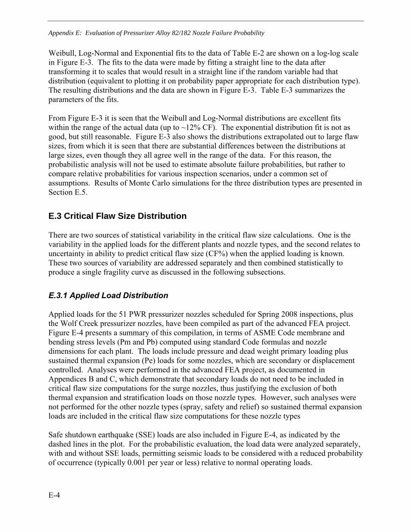
Appendix E: Evaluation of Pressurizer Alloy 82/182 Nozzle Failure Probability

E-4

Weibull, Log-Normal and Exponential fits to the data of Table E-2 are shown on a log-log scale in Figure E-3. The fits to the data were made by fitting a straight line to the data after transforming it to scales that would result in a straight line if the random variable had that distribution (equivalent to plotting it on probability paper appropriate for each distribution type). The resulting distributions and the data are shown in Figure E-3. Table E-3 summarizes the parameters of the fits.

From Figure E-3 it is seen that the Weibull and Log-Normal distributions are excellent fits within the range of the actual data (up to ~12% CF). The exponential distribution fit is not as good, but still reasonable. Figure E-3 also shows the distributions extrapolated out to large flaw sizes, from which it is seen that there are substantial differences between the distributions at large sizes, even though they all agree well in the range of the data. For this reason, the probabilistic analysis will not be used to estimate absolute failure probabilities, but rather to compare relative probabilities for various inspection scenarios, under a common set of assumptions. Results of Monte Carlo simulations for the three distribution types are presented in Section E.5.

E.3 Critical Flaw Size Distribution

There are two sources of statistical variability in the critical flaw size calculations. One is the variability in the applied loads for the different plants and nozzle types, and the second relates to uncertainty in ability to predict critical flaw size (CF%) when the applied loading is known. These two sources of variability are addressed separately and then combined statistically to produce a single fragility curve as discussed in the following subsections.

E.3.1 Applied Load Distribution

Applied loads for the 51 PWR pressurizer nozzles scheduled for Spring 2008 inspections, plus the Wolf Creek pressurizer nozzles, have been compiled as part of the advanced FEA project. Figure E-4 presents a summary of this compilation, in terms of ASME Code membrane and bending stress levels (Pm and Pb) computed using standard Code formulas and nozzle dimensions for each plant. The loads include pressure and dead weight primary loading plus sustained thermal expansion (Pe) loads for some nozzles, which are secondary or displacement controlled. Analyses were performed in the advanced FEA project, as documented in Appendices B and C, which demonstrate that secondary loads do not need to be included in critical flaw size computations for the surge nozzles, thus justifying the exclusion of both thermal expansion and stratification loads on those nozzle types. However, such analyses were not performed for the other nozzle types (spray, safety and relief) so sustained thermal expansion loads are included in the critical flaw size computations for these nozzle types

Safe shutdown earthquake (SSE) loads are also included in Figure E-4, as indicated by the dashed lines in the plot. For the probabilistic evaluation, the load data were analyzed separately, with and without SSE loads, permitting seismic loads to be considered with a reduced probability of occurrence (typically 0.001 per year or less) relative to normal operating loads.

Appendix E: Evaluation of Pressurizer Alloy 82/182 Nozzle Failure Probability

E-5

The data in Figure E-4 were sorted by increasing stress level, and were found to be well fit by Log-Normal statistical distributions, as illustrated in Figures E-5 and E-6 for Pm + Pb, with and without SSE loads, respectively. The fitting accuracy and parameters of the Log-normal fits are included on the figures.

E.3.2 Compilation of Full Scale Pipe Tests

The statistical fits of Figures E-5 and E-6 can be sampled to provide estimates of the distribution of applied loading on the pressurizer nozzles in the study. However, even if the applied loading were known with complete accuracy, uncertainty exists in our ability to predict the critical flaw size, in terms of CF%. To help characterize this uncertainty, a review was performed of test data from the NRC-sponsored Degraded Piping Program conducted at Battelle Columbus Laboratories [E-2, E-3]. Approximately 60 full scale pipe tests were conducted in this program, of pipes containing three types of circumferential defects: through-wall cracks, surface cracks, and complex cracks (see Figure E-7). Pipe sizes ranged from 4” to 42” and loadings included 4-point bending, combined bending + internal pressure and pure axial load. The majority of the pipes tested were in the 6” to 16” range which is directly relevant to the pressurizer nozzles being evaluated. Pipe materials in the tests included 304 stainless steel, Alloy 600 and Carbon Steel, but no pipes containing A-82 or 182 weldments were tested. Therefore the results of the predominantly base material pipe tests must be translated to DMWs on the basis of relative material properties for use in this evaluation. Fortunately, the piping materials used in the program were extensively characterized in terms of tensile properties and fracture toughness (J-R curves). Recent data also exists on the J-R properties of a large A-182 weldment, which can be used for comparison to the test materials.

Figure E-8 is a plot of test data from 31 of the pipe tests, performed on Austenitic materials only (304SS plus A-600). The data are plotted in terms of maximum loading achieved in the pipe tests (i.e. failure load) vs. % of pipe cross section cracked (CF %). The maximum load is plotted in terms of applied stress at the cracked cross section normalized by the ASME Section III design allowable stress for the appropriate test material (304 SS or A-600) and temperature, (Pm + Pb) / Sm.

The large majority of the tests in Figure E-8 were conducted under bending loading (Pb) only, and those tests yielded a very consistent trend. However, in order to include pipes tested under combined membrane plus bending (Pm + Pb), and since the applied nozzle loadings in Section E.3.1 include both membrane and bending loads, a correction factor was developed based on net section collapse analyses plus data from similar pipes tested under varying amounts of membrane and bending stress. Specifically, tests were conducted for some flaw geometries (surface flaws and WOL tests) under combined pressure plus bending loads. These were complemented by net section collapse analyses of the other flaw types (thru-wall and complex flaw geometries) to calculate the effective increase in total loading as a function of the relative fraction of Pm versus Pb in the test/analysis. The following correction factor for membrane stress was obtained:

(Pm + Pb)/Sm adjusted = [(Pm + Pb)/Sm] x [0.9817 + 0.4311 x Pm/(Pm + Pb)]

Appendix E: Evaluation of Pressurizer Alloy 82/182 Nozzle Failure Probability

E-6

which varies from ~1 for pure bending loading (Pm/(Pm + Pb) = 0) to ~1.4 for pure membrane loading (Pm/(Pm + Pb) = 1). Figure E-15 presents a plot of this correction factor, and the associated test and analysis data, which demonstrates an excellent correlation with the data.

Plotting the test results in this manner yields a monotonic trend with relatively little scatter, indicating that CF% is a reasonable parameter for characterization of the effect of cracking on pipe failure load, for the pipe and crack geometries tested, which are directly relevant to the subject nozzles. A power law fit of the data is shown on Figure E-8, which exhibits very good correlation and relatively little scatter for test data of this type. The equation and correlation coefficient of the fit are as follows:

(Pm + Pb)/Sm = 0.4061 (CF)-1.4613

R2 = 0.8988

E.3.3 Development of Fragility Curve

In order to develop a statistical distribution for this curve, residuals were calculated based on the difference between the actual CF for each data point and that predicted by the power law fit (CF – CFpredicted). The residuals were then sorted from lowest to highest, and were found to be reasonably represented by a normal distribution, as illustrated in Figure E-9. CF% was selected as the dependent variable in this correlation, since applied loading is the independent variable in the analysis (i.e. applied loads determined from the plant loading distributions are used to determine critical CF% from Figures E-8 and E-9).

Consistent with the advanced FEA project, the applied loads are first multiplied by a Z-factor [E-4] before entering Figures E-8 and E-9 which accounts for potentially lower toughness of Alloy-182 weldments relative to the austenitic base materials tested in the pipe tests. J-Resistance testing of a typical Alloy-182 weldment showed little or no reduction in toughness relative to the pipe test materials [E-4]. Sm for stainless steel base metal at pressurizer operating temperature was used to normalize the plant loads.

The final step in developing the fragility curve was to perform Monte Carlo sampling from the load distribution of Figure E-5, and then independently sample the critical flaw size distribution of Figures E-8 and E-9 for critical CF % for each load. Consideration was given to occasionally sampling from the SSE distribution of Figure E-6 (e.g. once in every 1000 simulations), however, the two distributions are so close that this was judged to have an insignificant effect. 1000 samples were performed, resulting in the critical flaw size distribution shown in Figure E-10. Both the sampling results and a Log-Normal fit to the distribution are plotted. The Log-Normal fit was found to give a very accurate representation of the fragility curve distribution. Parameters of the Log-Normal fit are also listed in Figure E-10.

One anomaly exists in the fragility curve in Figure E-10 which requires explanation. The curve yields a probability of failure of less than one for CF = 100%, which is physically impossible. This effect results from sampling the tails of the two distributions, which occasionally yields unrealistically small applied loads or unrealistically high critical flaw sizes (For example, the

Appendix E: Evaluation of Pressurizer Alloy 82/182 Nozzle Failure Probability

E-7

right hand side of the power law curve in Figure E-8 doesn’t go through zero.) However, this anomaly is corrected in the Monte Carlo analyses of Section E.5 by discarding and re-sampling any trials in which the critical flaw size is predicted to be greater than 100%.

E.4 Crack Growth

E.4.1 Summary of Advanced FEA Results

The advanced FEA analyses addressed a total of 53 cases with variations of each resulting in over 100 individual crack growth analyses. Over half of the analyses demonstrated stable crack arrest prior to penetrating through-wall or reaching critical size. The remainder exhibited varying degrees of crack growth. The first 20 cases were denoted base cases, and include cases that envelope all geometries and loads for the 51 Spring 2008 pressurizer nozzles. The 20 base cases and their resulting crack growth rates, in terms of CF% per year are summarized in Table E-4. (Note that a total of 22 analyses are actually reported in the table since two cases were run with two sets of weld residual stresses each.) The crack growth rates naturally divide into two regimes: crack growth from initial assumed flaw size until through wall (TW) penetration, denoted “Rate1” in the table, and crack growth following TW penetration, denoted “Rate2”. Rate2 can be seen to be on average about an order of magnitude greater than Rate1, indicating significant acceleration in crack growth once the assumed crack breaks through and becomes through wall.

Another observation from Table E-4 is that all but two base cases exhibit relatively small pre-TW crack growth rates (~1%/yr < Rate1 < 3.5%/yr) with the exception of Case 6 (9.85%/yr) and Case 17 (14.97%/yr). A similar trend is seen in the post-TW growth rates (Rate2), albeit at much higher rates. Thus for the geometries enveloped, the high crack growth rates predicted for cases 6 and 17 are relatively rare. The remainder of the cases (21 through 53) for the most part started with cases 6 and 17 and looked at the effect of various analysis parameters and assumptions on these bounding cases. For this reason, it was judged not appropriate to include these remaining cases in the statistical distribution of crack growth rates, since they would bias the distribution very much to the high side. Instead, only the base cases were used, but the spread in the distributions was combined with the experimental scatter in crack growth rates from MRP-115 [E-5], as described in the next section.

E.4.2 Adaptation to Probabilistic Analysis

The base case crack growth results identified in Section E.4.1 were used to define statistical distributions of crack growth rates for the probabilistic analysis. Figure E-11 presents the sorted data for pre- and post-penetration crack growth rates plotted versus cumulative probability. Bilinear fits to the data were developed for the two regions of each of the curves. These bilinear distributions properly characterize the dichotomy observed in the FEA results (i.e. about an 80% probability that the crack growth rate will be relatively small, and about a 20% probability of large crack growth rates as observed in Cases 6 and 17). The high portion of the crack growth distributions also extrapolate out to even higher crack growth rates than those predicted for Cases

Appendix E: Evaluation of Pressurizer Alloy 82/182 Nozzle Failure Probability

E-8

6 and 17, thereby covering to some extent the remaining sensitivity cases that weren’t included in the distribution.

The distributions in Figure E-11 do not include the scatter in the crack growth rate itself. All the base case computations used the 75th percentile of the MRP-155 crack growth rate distribution that describes material crack growth rate scatter (Figure E-12).

The material crack growth rate scatter needs to be combined with the above analytical distributions to obtain the overall statistical description of the crack growth rate. This was accomplished by Monte Carlo simulation employing the following steps:

1. Sample from the bilinear distributions of Figure E-11.

2. Divide the sampled value by the ratio of the 75th to the 50th percentile of the MRP-115 distribution of Figure E-12(i.e. adjust to the median).

3. Sample from the MRP distribution (with a median of 1 and lognormal shape parameter of 0.6069) to determine a multiplier for the analytical crack growth rate.

4. Multiply the sample from Step 2 by the sample from Step 3.

This provides a set of samples from which a cumulative distribution can be derived. The cumulative distribution for pre-TW penetration is shown in Figure E-13 on lognormal scales (as data points) along with a lognormal distribution that was fit to the data. The line is seen to provide a good description to the Monte Carlo results. The constants describing the line are the parameters of the lognormal distribution of crack growth rate for pre-penetration.

A similar analysis was performed for the post-TW penetration data. Figure E-14 provides the corresponding results.

Note that, for purposes of this analysis, it was not considered necessary to include new crack initiations or multiple crack initiations during the evaluation periods. These are considered to be adequately addressed by starting with the empirical nozzle flaw distributions derived in Section E.2.

E.5 Monte Carlo Analysis

Monte Carlo simulation was used to generate results of the probability of a nozzle failure as a function of time.

E.5.1 Methodology

The following steps were used in each trial of the Monte Carlo simulation.

1. SAMPLE CRACK SIZE (CF%) from one of the flaw size distributions (Weibull, Log-Normal, Exponential) developed in Section E.2. Truncate the CF at 100% (if the sampled

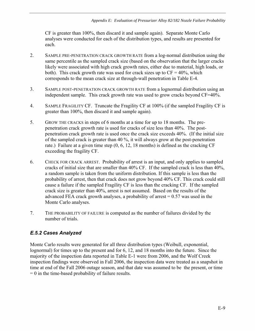
Appendix E: Evaluation of Pressurizer Alloy 82/182 Nozzle Failure Probability

E-9

CF is greater than 100%, then discard it and sample again). Separate Monte Carlo analyses were conducted for each of the distribution types, and results are presented for each.

2. SAMPLE PRE-PENETRATION CRACK GROWTH RATE from a log-normal distribution using the same percentile as the sampled crack size (based on the observation that the larger cracks likely were associated with high crack growth rates, either due to material, high loads, or both). This crack growth rate was used for crack sizes up to CF = 40%, which corresponds to the mean crack size at through-wall penetration in Table E-4.

3. SAMPLE POST-PENETRATION CRACK GROWTH RATE from a lognormal distribution using an independent sample. This crack growth rate was used to grow cracks beyond CF=40%.

4. SAMPLE FRAGILITY CF. Truncate the Fragility CF at 100% (if the sampled Fragility CF is greater than 100%, then discard it and sample again).

5. GROW THE CRACKS in steps of 6 months at a time for up to 18 months. The pre-penetration crack growth rate is used for cracks of size less than 40%. The post-penetration crack growth rate is used once the crack size exceeds 40%. (If the initial size of the sampled crack is greater than 40 %, it will always grow at the post-penetration rate.) Failure at a given time step (0, 6, 12, 18 months) is defined as the cracking CF exceeding the fragility CF.

6. CHECK FOR CRACK ARREST. Probability of arrest is an input, and only applies to sampled cracks of initial size that are smaller than 40% CF. If the sampled crack is less than 40%, a random sample is taken from the uniform distribution. If this sample is less than the probability of arrest, then that crack does not grow beyond 40% CF. This crack could still cause a failure if the sampled Fragility CF is less than the cracking CF. If the sampled crack size is greater than 40%, arrest is not assumed. Based on the results of the advanced FEA crack growth analyses, a probability of arrest = 0.57 was used in the Monte Carlo analyses.

7. THE PROBABILITY OF FAILURE is computed as the number of failures divided by the number of trials.

E.5.2 Cases Analyzed

Monte Carlo results were generated for all three distribution types (Weibull, exponential, lognormal) for times up to the present and for 6, 12, and 18 months into the future. Since the majority of the inspection data reported in Table E-1 were from 2006, and the Wolf Creek inspection findings were observed in Fall 2006, the inspection data were treated as a snapshot in time at end of the Fall 2006 outage season, and that date was assumed to be the present, or time = 0 in the time-based probability of failure results.

Appendix E: Evaluation of Pressurizer Alloy 82/182 Nozzle Failure Probability

E-10

E.5.3 Results

The results of the Monte Carlo simulations are presented in Table E-5. 107 trials were used in each case. The cumulative probabilities are directly from the Monte Carlo simulation and are given for each of the three distribution-types. The incremental probabilities are the differences in the cumulative probabilities for each six-month time span. These correspond to the probability of a nozzle rupture (per nozzle) during each six-month time interval.

The number of nozzles column corresponds to the number of remaining, PWSCC-susceptible pressurizer nozzles that will not have been inspected or mitigated at the end of each outage season, assuming that the industry inspection plans are implemented. The next column reflects the number of plants containing those uninspected/unmitigated nozzles. The probability of a nozzle failure in the time increment is given by the expression Pnoz=1-(1-p1)N, where p1 is the incremental failure probability for a single nozzle and N is the number of nozzles. The per plant probability of a nozzle failure is then obtained by dividing by the number of plants in which those nozzles exist.

It may be observed from Table E-5 that the incremental probabilities of nozzle failure are remaining about constant for each of the six month intervals, especially for the analyses performed with the Weibull and lognormal flaw distributions (which from Figure E-2 were the better fits of the data). The analyses with the exponential distribution show some increase in incremental probability of failure versus time, but those start at much lower present values (time = 0), since the exponential fit produced less conservative extrapolations of probabilities of larger flaw sizes. Since the numbers of susceptible nozzles and plants are being removed from the population at a steady rate, the industry inspection plan results in an essentially constant probability of a nozzle failure per time interval, until the time when all nozzles will have been inspected or mitigated, at the end of the Spring 2008 outage season.

E.6 Conclusions

The following observations are offered based on the results of the probabilistic evaluation presented in Table E-5:

• Pressurizer nozzle failure probabilities (per plant, per six months) for the Spring-08 Plants are approximately the same as what has existed in PWRs due to PWSCC susceptible pressurizer nozzles during the Fall and Spring of 2007 (on the order of 4 x 10-3 per plant, per six months). During 2007, this failure probability existed for the entire year, resulting in an estimated failure probability (per plant per year) of ~8 x 10-3. For 2008, this probability will exist for less than six months; so on a per reactor-year basis, the failure probability will actually be a factor of two smaller in 2008.

• The absolute failure probabilities resulting from this study are greater than generally accepted LOCA frequencies. However, as stated in Section E.2, the results of the probabilistic evaluation are not intended to yield absolute probabilities for comparison to fixed licensing limits, but rather, are intended to provide estimates of the relative effects of various inspection programs, such as accelerating the Spring 2008 exams versus not

Appendix E: Evaluation of Pressurizer Alloy 82/182 Nozzle Failure Probability

E-11

accelerating them. Furthermore, these results assume no leakage or plant response to leakage. For comparison to accepted LOCA probabilities, they need to be factored by the probability of non-Leak-Before-Break (or failure to react to leakage), which is expected to be very small, given the increased attention to the PWSCC concern in these particular plants and nozzles, and the associated confirmatory action commitments by the utilities relative to leakage monitoring and immediate plant actions if leakage is detected..

• Based on the advanced FEA analyses performed in the body of this report, plus the above referenced confirmatory action commitments, it is extremely unlikely that leaks from these nozzle locations would go undetected for a sufficient duration and of sufficient magnitude that a break could occur before operator action to shut the plant down. A total of 108 crack growth analysis cases were performed in the main sensitivity matrix and all 108 cases showed either stable crack arrest or crack leakage and stability results that satisfied agreed-upon evaluation criteria. In most cases, the results showed large margins relative to those criteria. Many of the cases were conservative sensitivity studies that utilized limiting base case results as their starting point, and thus the 108 case matrix (plus several supplemental cases that were added) represent a conservatively biased sample of the actual nozzle population. On this basis, a reasonable estimate of the probability of a leak going undetected to the point of pipe rupture in one of the subject nozzles is estimated to be on the order of 1/500 (assuming that an unbiased matrix of the actual nozzle population would add an additional 400 arrests or acceptable cases). Applying this probability to the probability of nozzle rupture, assuming no LBB, for the Spring 2008 plants of 1.6 x 10-3 to 4 x 10-3 (Table E-4) results in a combined probability of pipe rupture of 8 x 10-6 to 2 x 10-5

per reactor-year for the nine Spring 2008 plants.

On the basis of these evaluation results, it is concluded that there is no significant benefit, in terms of reduced nozzle failure probability, to accelerating the originally scheduled Spring 2008 inspections. The probability of nozzle failure, assuming no leak before break, is predicted to be less for the Spring 2008 plants than it was, on a per-plant-year basis, for the plants that inspected/mitigated in Spring or Fall of 2007. The results of this study are complementary to the advanced FEA program discussed in the body of the report, in that they provide an indication of what to expect for the very small number of cases in which leak-before-break cannot be demonstrated.

E.7 References

E-1. Materials Reliability Program: Primary System Piping Butt Weld Inspection and Evaluation Guidelines (MRP-139), EPRI, Palo Alto, CA: 2005. 1010087.

E-2. Summary of Technical Results and Their Significance to Leak-Before-Break and In-Service Flaw Acceptance Criteria, NUREG/CR-4082, Volume 8, March 1984 - January 1989.

E-3. Pipe Fracture Encyclopedia, U.S. NRC, 1997 (A collection of NUREG Reports and Data Files from the DP2 and other programs distributed on CDs).

Appendix E: Evaluation of Pressurizer Alloy 82/182 Nozzle Failure Probability

E-12

E-4. G. Wilkowski, H. Xu, D.-J. Shim, and D. Rudland, “Determination of the Elastic-Plastic Fracture Mechanics Z-factor for Alloy 82/182 Weld Metal Flaws for Use in the ASME Section XI Appendix C Flaw Evaluation Procedures,” PVP2007-26733, Proceedings of ASME-PVP 2007: 2007 ASME Pressure Vessels and Piping Division Conference, San Antonio, TX, 2007.

E-5. Materials Reliability Program (MRP) Crack Growth Rates for Evaluating Primary Water Stress Corrosion Cracking (PWSCC) of Alloy 82, 182, and 132 Welds (MRP-115), EPRI, Palo Alto, CA: 2004. 1006696.

Appendix E: Evaluation of Pressurizer Alloy 82/182 Nozzle Failure Probability

E-13

Table E-1 Plant Data used in Flaw Distribution

Plant Inspection Date Nozzle OD

(in) Thick (t, in)

Type of Indication

IndicationDepth (a, in)

Indication Length (l, in)

a/t l/circ Criticality Factor

Tihange 2 2002 Surge 14 1.4 Axial 0.600 0.000 43% 0% 0.00% TMI 2003 Surge 12 1.3 Axial 0.585 0.000 45% 0% 0.00%

Tsuruga 2003 Relief 6 1 Axial 1.000 0.000 100% 0% 0.00% Tsuruga 2003 Safety 6 1 Axial 0.900 0.000 90% 0% 0.00% Calvert 2 2005 CL Drain 2 0.56 Circ 0.056 0.628 10% 10% 1.00% Calvert 2 2005 HL Drain 2 0.56 Axial 0.392 0.000 70% 0% 0.00% DC Cook 2005 Safety 8 1.4 Axial 1.232 0.000 88% 0% 0.00% Farley 2 2005 Safety 8 1.1 Clean 0.000 0.000 0% 0% 0.00% Farley 2 2005 Spray 6 0.83 Clean 0.000 0.000 0% 0% 0.00% Calvert 1 2006 HL Drain 2.875 0.54 Circ 0.100 0.450 19% 5% 0.92% Calvert 1 2006 Relief 6.0675 1.3 Axial 0.100 0.000 8% 0% 0.00% Calvert 1 2006 Surge 12.75 1.6 Circ 0.400 2.400 25% 6% 1.50%

Davis Besse 2006 CL Drain 2 0.56 Axial 0.056 0.000 7% 0% 0.00%

D-B 2006 Relief 4.5 0.8125 Clean 0.000 0.000 0% 0% 0.00% D-B 2006 Safety 4.5 0.8125 Clean 0.000 0.000 0% 0% 0.00% D-B 2006 Safety 4.5 0.8125 Clean 0.000 0.000 0% 0% 0.00% D-B 2006 Spray 5.125 0.625 Clean 0.000 0.000 0% 0% 0.00% D-B 2006 Surge 11.5 1.125 Clean 0.000 0.000 0% 0% 0.00%

Prairie Is. 2006 Surge 15 1.5 Clean 0.000 0.000 0% 0% 0.00% SONGS 2 2006 Safety 8 1.4 Axial 0.420 0.000 30% 0% 0.00% SONGS 2 2006 Safety 8 1.4 Axial 0.420 0.000 30% 0% 0.00% SONGS 2 2006 Safety 8 1.4 Clean 0.000 0.000 0% 0% 0.00% SONGS 2 2006 Spray 5.5 0.75 Clean 0.000 0.000 0% 0% 0.00% SONGS 3 2006 Relief 8 1.1875 Clean 0.000 0.000 0% 0% 0.00% SONGS 3 2006 Safety 8 1.1875 Clean 0.000 0.000 0% 0% 0.00% SONGS 3 2006 Safety 8 1.1875 Clean 0.000 0.000 0% 0% 0.00% SONGS 3 2006 Spray 5.5 0.75 Clean 0.000 0.000 0% 0% 0.00% SONGS 3 2006 Surge 13 1.437 Clean 0.000 0.000 0% 0% 0.00% Watts Bar 2006 Relief 7.75 1.29 Clean 0.000 0.000 0% 0% 0.00% Watts Bar 2006 Safety 7.75 1.29 Clean 0.000 0.000 0% 0% 0.00% Watts Bar 2006 Safety 7.75 1.29 Clean 0.000 0.000 0% 0% 0.00% Watts Bar 2006 Safety 7.75 1.29 Clean 0.000 0.000 0% 0% 0.00% Watts Bar 2006 Spray 6 0.9 Clean 0.000 0.000 0% 0% 0.00% Watts Bar 2006 Surge 15 1.5 Clean 0.000 0.000 0% 0% 0.00%

Wolf Creek 2006 Relief 7.96 1.32 Circ 0.340 11.500 25.8% 46% 11.85% Wolf Creek 2006 Safety 7.96 1.32 Circ 0.297 2.500 22.5% 10% 2.25% Wolf Creek 2006 Safety 7.96 1.32 Clean 0.000 0.000 0% 0% 0.00% Wolf Creek 2006 Safety 7.96 1.32 Clean 0.000 0.000 0% 0% 0.00% Wolf Creek 2006 Spray 6 0.9 Clean 0.000 0.000 0% 0% 0.00% Wolf Creek 2006 Surge 15 1.45 Circ 0.465 8.750 32.1% 19% 5.95%

Farley 2 2007 Safety 8 1.1 Clean 0.000 0.000 0% 0% 0.00% Farley 2 2007 Safety 8 1.1 Clean 0.000 0.000 0% 0% 0.00% Farley 2 2007 Safety 8 1.1 Clean 0.000 0.000 0% 0% 0.00% Farley 2 2007 Safety 8 1.1 Clean 0.000 0.000 0% 0% 0.00%

Appendix E: Evaluation of Pressurizer Alloy 82/182 Nozzle Failure Probability

E-14

Table E-1 Plant Data used in Flaw Distribution (cont’d)

Plant Inspection Date Nozzle OD

(in) Thick (t, in)

Type of Indication

IndicationDepth (a, in)

Indication Length (l, in)

a/t l/circ Criticality Factor

Farley 2 2007 Spray 6 0.83 Clean 0.000 0.000 0% 0% 0.00% Farley 2 2007 Surge 15 1.52 Circ 0.500 3.000 33% 6% 2.12% Calvert 2 2007 Safety 8 1.1875 Clean 0.117 1.886 0% 0% 0.00% Calvert 2 2007 Safety 8 1.1875 Clean 0.052 1.681 0% 0% 0.00% Calvert 2 2007 Spray 5.5 0.75 Clean 0.066 1.475 0% 0% 0.00% Calvert 2 2007 Surge 13 1.437 Clean 0.030 3.107 0% 0% 0.00%

Table E-2 Circumferential Indications from Table E-1 Including Estimates of Cumulative Probability

CF Rank,

i F,

i/N* 1-F

0.92% 7 0.14 0.86

1.00% 6 0.12 0.88

1.50% 5 0.1 0.9

2.09% 4 0.08 0.92

2.25% 3 0.06 0.94

5.95% 2 0.04 0.96

11.85% 1 0.02 0.98

* N = 51

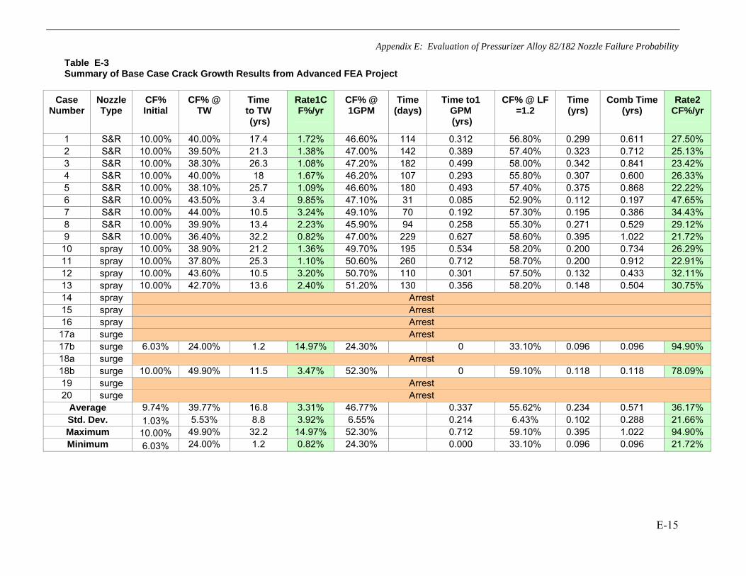
Appendix E: Evaluation of Pressurizer Alloy 82/182 Nozzle Failure Probability

E-15

Table E-3 Summary of Base Case Crack Growth Results from Advanced FEA Project

Case Number

Nozzle Type

CF% Initial

CF% @ TW

Time to TW (yrs)

Rate1CF%/yr

CF% @ 1GPM

Time(days)

Time to1 GPM (yrs)

CF% @ LF =1.2

Time (yrs)

Comb Time(yrs)

Rate2 CF%/yr

1 S&R 10.00% 40.00% 17.4 1.72% 46.60% 114 0.312 56.80% 0.299 0.611 27.50% 2 S&R 10.00% 39.50% 21.3 1.38% 47.00% 142 0.389 57.40% 0.323 0.712 25.13% 3 S&R 10.00% 38.30% 26.3 1.08% 47.20% 182 0.499 58.00% 0.342 0.841 23.42% 4 S&R 10.00% 40.00% 18 1.67% 46.20% 107 0.293 55.80% 0.307 0.600 26.33% 5 S&R 10.00% 38.10% 25.7 1.09% 46.60% 180 0.493 57.40% 0.375 0.868 22.22% 6 S&R 10.00% 43.50% 3.4 9.85% 47.10% 31 0.085 52.90% 0.112 0.197 47.65% 7 S&R 10.00% 44.00% 10.5 3.24% 49.10% 70 0.192 57.30% 0.195 0.386 34.43% 8 S&R 10.00% 39.90% 13.4 2.23% 45.90% 94 0.258 55.30% 0.271 0.529 29.12% 9 S&R 10.00% 36.40% 32.2 0.82% 47.00% 229 0.627 58.60% 0.395 1.022 21.72% 10 spray 10.00% 38.90% 21.2 1.36% 49.70% 195 0.534 58.20% 0.200 0.734 26.29% 11 spray 10.00% 37.80% 25.3 1.10% 50.60% 260 0.712 58.70% 0.200 0.912 22.91% 12 spray 10.00% 43.60% 10.5 3.20% 50.70% 110 0.301 57.50% 0.132 0.433 32.11% 13 spray 10.00% 42.70% 13.6 2.40% 51.20% 130 0.356 58.20% 0.148 0.504 30.75% 14 spray Arrest 15 spray Arrest 16 spray Arrest

17a surge Arrest 17b surge 6.03% 24.00% 1.2 14.97% 24.30% 0 33.10% 0.096 0.096 94.90% 18a surge Arrest 18b surge 10.00% 49.90% 11.5 3.47% 52.30% 0 59.10% 0.118 0.118 78.09% 19 surge Arrest 20 surge Arrest

Average 9.74% 39.77% 16.8 3.31% 46.77% 0.337 55.62% 0.234 0.571 36.17% Std. Dev. 1.03% 5.53% 8.8 3.92% 6.55% 0.214 6.43% 0.102 0.288 21.66% Maximum 10.00% 49.90% 32.2 14.97% 52.30% 0.712 59.10% 0.395 1.022 94.90% Minimum 6.03% 24.00% 1.2 0.82% 24.30% 0.000 33.10% 0.096 0.096 21.72%

Appendix E: Evaluation of Pressurizer Alloy 82/182 Nozzle Failure Probability

E-16

Table E-4 Parameters of the Fitted Distributions

Distribution Type

Complementary Cumulative Distribution

Values of Parameters

R2

Exponential bxCe /− 1/b = 16.293, C= 0.1225

0.9052

Weibull βη )/( xe− β=0.2543, η=0.000539

0.9704

Log-Normal

21

erfc ⎥⎦

⎤⎢⎣

⎡2

)/ln(σ

mx

m = 0.0040365, σ= 2.775745

0.9704

Table E-5 Results of Monte Carlo Simulation

Distribution/ Outage Season

Time (months)

Time Increment (months)

Cumulative Prob.

Incremental Prob. (pi)

# Nozzles (N)

# Plants (NP)

Nozzle Failure Probability

Total* per Plant** Weibull Fall-06 0 6.4380E-04 278 50

Spring-07 6 6 1.3855E-03 7.42E-04 195 34 0.1347 0.0040Fall-07 12 6 2.1573E-03 7.72E-04 121 21 0.0892 0.0042

Spring-08 18 6 2.8700E-03 7.13E-04 51 9 0.0357 0.0040

Log Normal Fall-06 0 8.5860E-04 278 50

Spring-07 6 6 1.7445E-03 8.86E-04 195 34 0.1587 0.0047Fall-07 12 6 2.5585E-03 8.14E-04 121 21 0.0938 0.0045

Spring-08 18 6 3.2759E-03 7.17E-04 51 9 0.0359 0.0040

Exponential Fall-06 0 2.1000E-06 278 50

Spring-07 6 6 3.1500E-05 2.94E-05 195 34 0.0057 0.0002Fall-07 12 6 1.5300E-04 1.22E-04 121 21 0.0146 0.0007

Spring-08 18 6 4.4470E-04 2.92E-04 51 9 0.0148 0.0016

*Total Failure Prob. = 1 – (1-pi)N **Failure Prob. Per Plant = Total Prob./NP

Appendix E: Evaluation of Pressurizer Alloy 82/182 Nozzle Failure Probability

E-17

0

0.1

0.2

0.3

0.4

0.5

0.6

0.7

0.8

0.9

1

0% 10% 20% 30% 40% 50% 60% 70% 80% 90% 100%

CF(%)

Prob

abili

ty

Weib Flaw distFragility6 Mo Growth12 Mo Growth18 Mo Growth

(a)

0

0.005

0.01

0.015

0.02

0.025

0.03

0.035

0.04

0.045

0.05

0% 10% 20% 30% 40% 50% 60% 70% 80% 90% 100%

CF (%)

Prob

abili

ty

Weib Flaw distFragility6 Mo Growth12 Mo Growth18 Mo Growth

(b)

Figure E-1 a) Complementary Cumulative Distribution of Crack Area Fraction at Different Times, along with Complementary Cumulative Distribution of Critical Crack Area Fraction (CF, %) b) Enlargement of Low Probability Region of Figure E-1a

Appendix E: Evaluation of Pressurizer Alloy 82/182 Nozzle Failure Probability

E-18

0%

10%

20%

30%

40%

50%

60%

70%

80%

90%

100%

0% 10% 20% 30% 40% 50% 60% 70% 80% 90% 100%

l/circumference

a/th

ickn

ess

DMW Indications

WOLF Creek Indications

Farley Surge Nozzle

Crit-50th %-tile

Crit-99.9th %-tile

Clean Inspections

Axial Indications

Circumferenial Indications

Figure E-2 Plot of Indication Sizes along with 50th and 99.9th Percentiles of Fragility Curve

0.001

0.01

0.1

1

0.10% 1.00% 10.00% 100.00%

CF (%)

Prob

abili

ty 1-WeibExp FitLN FitData

Figure E-3 Complementary Cumulative Distributions of CF Showing Each of the Three Fits along with the Data

Appendix E: Evaluation of Pressurizer Alloy 82/182 Nozzle Failure Probability

E-19

0

4

8

12

16

01 A

- R

e (7

.75x

5.17

)

02 A

- SA

(7.7

5x5.

17)

03 A

- SB

(7.7

5x5.

17)

04 A

- SC

(7.7

5x5.

17)

05 E

- R

e (7

.75x

5.17

)

06 E

- SA

(7.7

5x5.

17)

07 E

- SB

(7.7

5x5.

17)

08 E

- SC

(7.7

5x5.

17)

09 H

- R

e (7

.75x

5.17

)

10 H

- SA

(7.7

5x5.

17)

11 H

- SB

(7.7

5x5.

17)

12 H

- SC

(7.7

5x5.

17)

WC

1 J

- Re

(7.7

5x5.

17)

WC

1a J

- R

e/Sa

(7.7

5x5.

17)

WC

2 J

- SA

(7.7

5x5.

17)

WC

3 J

- SB

(7.7

5x5.

17)

WC

4 J

- SC

(7.7

5x5.

17)

13 F

- R

e (8

x5.1

9)

14 F

- SA

(8x5

.19)

15 F

- SB

(8x5

.19)

16 F

- SC

(8x5

.19)

17 B

- R

e (7

.75x

5.62

)

18 B

- SA

(7.7

5x5.

62)

19 B

- SB

(7.7

5x5.

62)

20 B

- SC

(7.7

5x5.

62)

21 G

- R

e (7

.75x

5.62

)

22 G

- SA

(7.7

5x5.

62)

23 G

- SB

(7.7

5x5.

62)

24 G

- SC

(7.7

5x5.

62)

25 C

- R

e (7

.75x

5.62

)

26 C

- SA

(7.7

5x5.

62)

27 C

- SB

(7.7

5x5.

62)

28 C

- SC

(7.7

5x5.

62)

29 D

- R

e (8

x5.1

9)

30 D

- SA

(8x5

.19)

31 D

- SB

(8x5

.19)

32 D

- SC

(8x5

.19)

33 I

- Re

(8x5

.188

)

34 I

- SA

(8x5

.188

)

35 I

- SB

(8x5

.188

)

36 A

- Sp

(5.8

1x4.

01)

37 E

- Sp

(5.8

1x4.

01)

WC

5 J

- Sp

(5.8

1x4.

01)

38 B

- Sp

(5.8

1x4.

25)

39 G

- Sp

(5.8

1x4.

25)

40 C

- Sp

(5.8

1x4.

25)

41 F

- Sp

(8x5

.695

)

42 D

- Sp

(5.1

88x3

.062

)

43 I

- Sp

(5.1

88x3

.25)

44 A

- Su

(15x

11.8

44)

45 E

- Su

(15x

11.8

44)

46 H

- Su

(15x

11.8

44)

WC

6 J

- Su

(15x

11.8

44)

47 B

- Su

(15x

11.8

44)

48 G

- Su

(15x

11.8

44)

49 C

- Su

(15x

11.8

75)

50 D

- Su

(13.

063x

10.1

25)

51 I

- Su

(13.

063x

10.1

25)

P m+ P

b S

tres

s Lo

adin

g (k

si)

0

0.1

0.2

0.3

0.4

0.5

0.6

0.7

0.8

0.9

10.0

00.7

51.5

02.2

53.0

03.7

54.5

05.2

56.0

06.7

57.5

08.2

59.5

010

.2511

.0011

.7512

.5013

.2514

.0014

.7515

.5016

.2517

.0017

.7518

.5019

.2520

.0020

.7521

.5022

.2523

.0023

.7524.5

025.2

526

.0026

.7527

.5028

.2529

.0029

.7530

.5031

.2532

.0032

.7533

.5034

.2535

.0035

.7536

.5037

.2538

.0038

.7539

.5040

.2541

.0041

.7542

.5043

.2544

.0044

.7545

.5046

.2547

.0047

.7548

.5049

.2550

.0050

.7551

.5052

.2553

.0053

.7554

.5055

.2556

.0056

.7557

.5058

.2559

.0059

.75

Pm+PbPm+Pb with SSE

Figure E-4 Compilation of Applied Stresses (Pm + Pb) in 51 Pressurizer Nozzles scheduled for Spring 2008 Inspection plus Wolf Creek, with and without SSE seismic stresses. Data for Spray, safety and relief nozzles include thermal expansion loads, data for surge nozzles include primary stresses only.

Log Norm Fit (w/o SSE)

R2 = 0.9672

0.000

0.500

1.000

1.500

2.000

2.500

3.000

-2.500 -2.000 -1.500 -1.000 -0.500 0.000 0.500 1.000 1.500 2.000 2.500

Norm Dist.

LN (P

m +

Pb+

Pe)

w/o

SSE

Median = 7.8 ksiMean (ln) = 2.055Std. Dev. (ln) = 0.283

Figure E-5 Log-normal Fit and Parameters of Applied Load Distribution without Seismic Loads

Appendix E: Evaluation of Pressurizer Alloy 82/182 Nozzle Failure Probability

E-20

Log Normal Fit w/SSE

R2 = 0.9828

0.000

0.500

1.000

1.500

2.000

2.500

3.000

3.500

-2.500 -2.000 -1.500 -1.000 -0.500 0.000 0.500 1.000 1.500 2.000 2.500

Norm Dist.

LN (P

m +

Pb

+ Pe

) w/ S

SE)

Median = 9.2 ksiMean (ln) = 2.237Std. Dev. (ln) = 0.334

Figure E-6 Log-normal Fit and Parameters of Applied Load Distribution without Seismic Loads

Figure E-7 Illustration of Circumferential Flaw Types Tested in Degraded Piping Program Full Scale Pipe Tests

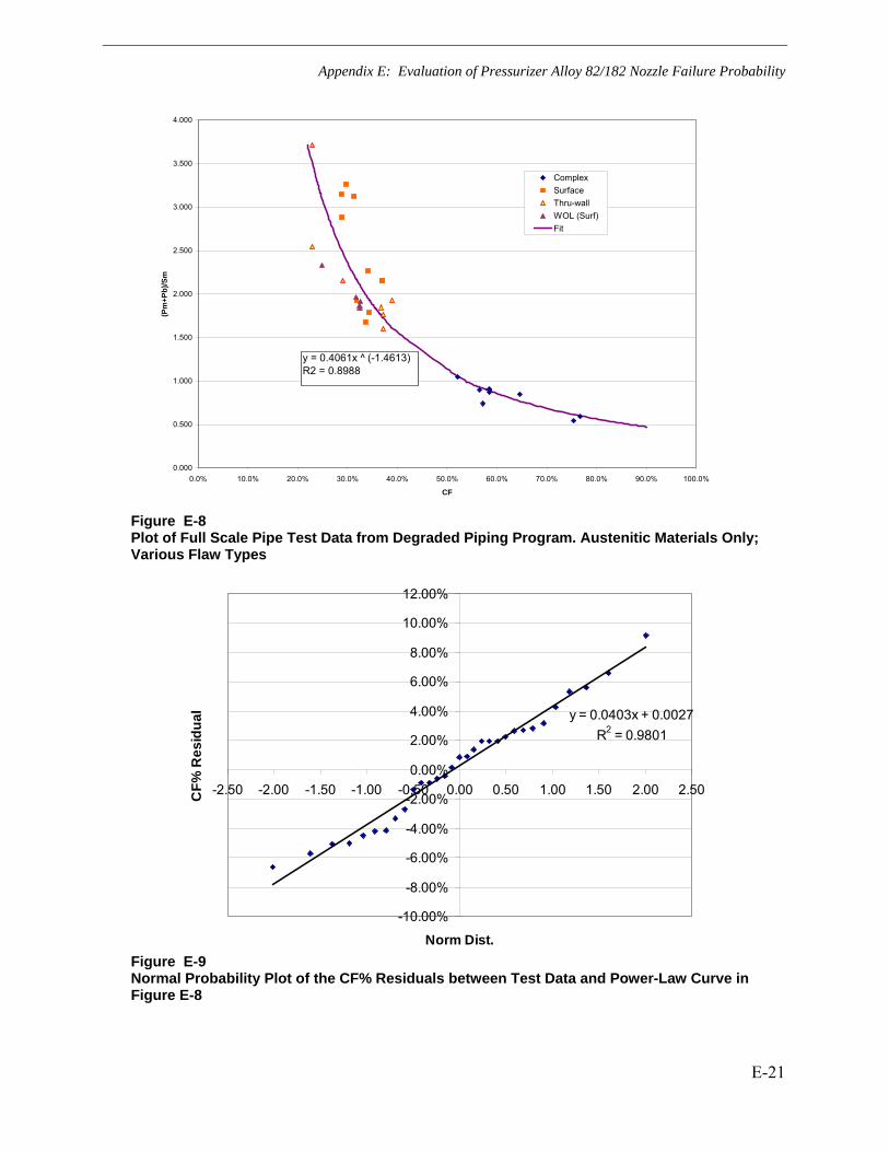
Appendix E: Evaluation of Pressurizer Alloy 82/182 Nozzle Failure Probability

E-21

0.000

0.500

1.000

1.500

2.000

2.500

3.000

3.500

4.000

0.0% 10.0% 20.0% 30.0% 40.0% 50.0% 60.0% 70.0% 80.0% 90.0% 100.0%

CF

(Pm

+Pb)

/Sm

ComplexSurfaceThru-wallWOL (Surf)Fit

y = 0.4061x ̂(-1.4613)R2 = 0.8988

Figure E-8 Plot of Full Scale Pipe Test Data from Degraded Piping Program. Austenitic Materials Only; Various Flaw Types

y = 0.0403x + 0.0027R2 = 0.9801

-10.00%

-8.00%

-6.00%

-4.00%

-2.00%

0.00%

2.00%

4.00%

6.00%

8.00%

10.00%

12.00%

-2.50 -2.00 -1.50 -1.00 -0.50 0.00 0.50 1.00 1.50 2.00 2.50

Norm Dist.

CF%

Res

idua

l

Figure E-9 Normal Probability Plot of the CF% Residuals between Test Data and Power-Law Curve in Figure E-8

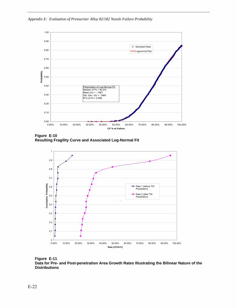
Appendix E: Evaluation of Pressurizer Alloy 82/182 Nozzle Failure Probability

E-22

0.00

0.10

0.20

0.30

0.40

0.50

0.60

0.70

0.80

0.90

1.00

0.00% 10.00% 20.00% 30.00% 40.00% 50.00% 60.00% 70.00% 80.00% 90.00% 100.00%

CF % at Failure

Prob

abili

ty

Sampled Data

Lognormal Dist.

Parameters of Log-Normal Fit:Median CF% = 82.5%Mean (ln) = -.1967Std. Dev. (ln) = .1969R^2 of Fit = 0.999

Figure E-10 Resulting Fragility Curve and Associated Log-Normal Fit

0

0.1

0.2

0.3

0.4

0.5

0.6

0.7

0.8

0.9

1

0.00% 10.00% 20.00% 30.00% 40.00% 50.00% 60.00% 70.00% 80.00% 90.00% 100.00%

Rate (CF%/Yr)

Cum

ulat

ive

Pro

babi

lity

Rate 1 (before TWPenetration)

Rate 2 (after TWPenetration)

``

Figure E-11 Data for Pre- and Post-penetration Area Growth Rates Illustrating the Bilinear Nature of the Distributions

Appendix E: Evaluation of Pressurizer Alloy 82/182 Nozzle Failure Probability

E-23

0.00

0.25

0.50

0.75

1.00

0.10 1.00 10.00CGR Multiplier

Prob

abili

ty

LogNormData

Figure E-12 MRP-115 Distribution Characterizing Material Crack Growth Rate Scatter for PWSCC in Alloy 182 Weld Metal

-3

-2

-1

0

1

2

3

0.10% 1.00% 10.00% 100.00%

CGR before TW Penetration (CF%/yr)

Nor

mal

Dis

t

Lognormal Parameters:Mean (ln) = -4.30984STD (ln) = 0.992779

Median Growth Rate = 1.34%/yr

Figure E-13 Monte Carlo Simulation Results of Pre-TW Penetration Crack Growth Rates with Fitted Lognormal Line

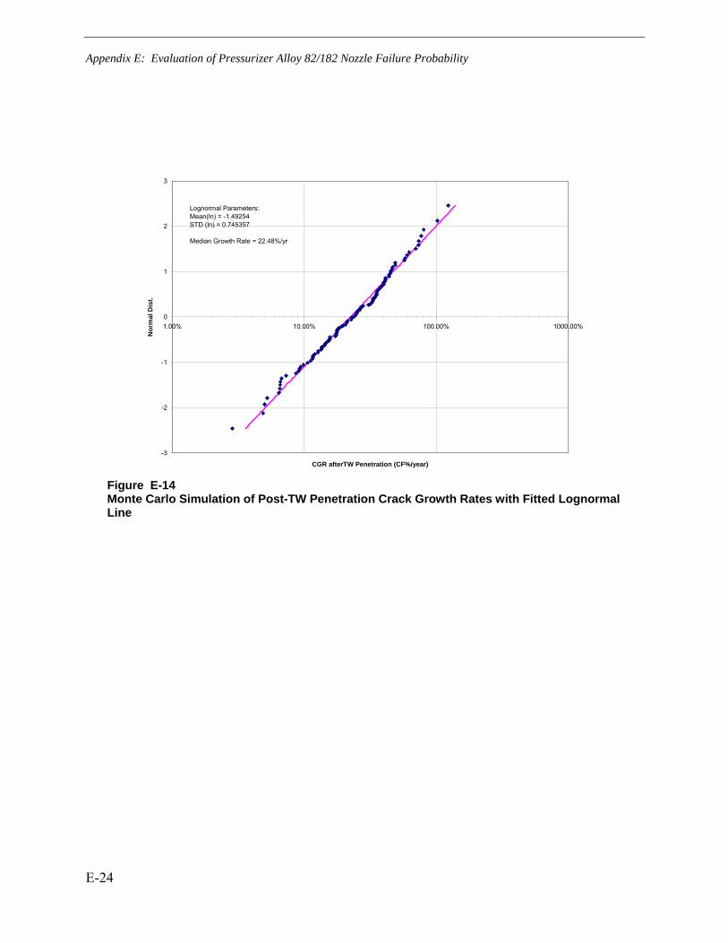
Appendix E: Evaluation of Pressurizer Alloy 82/182 Nozzle Failure Probability

E-24

-3

-2

-1

0

1

2

3

1.00% 10.00% 100.00% 1000.00%

CGR afterTW Penetration (CF%/year)

Nor

mal

Dis

t.

Lognormal Parameters:Mean(ln) = -1.49254STD (ln) = 0.745357

Median Growth Rate = 22.48%/yr

Figure E-14 Monte Carlo Simulation of Post-TW Penetration Crack Growth Rates with Fitted Lognormal Line