Monitoring a Building Using Deconvolution Interferometry. II: Ambient-

Vibration Analysis

by Nori Nakata and Roel Snieder

Abstract Application of deconvolution interferometry to earthquake data recordedinside a building is a powerful technique for monitoring parameters of the building,such as velocities of traveling waves, frequencies of normal modes, and intrinsicattenuation. In this study, we apply interferometry to ambient-vibration data, insteadof using earthquake data, to monitor a building. The time continuity of ambientvibrations is useful for temporal monitoring. We show that, because multiple sourcessimultaneously excite vibrations inside the building, the deconvolved waveformsobtained from ambient vibrations are nonzero for both positive and negative times,unlike the purely causal waveforms obtained from earthquake data. We develop astring model to qualitatively interpret the deconvolved waveforms. Using the syntheticwaveforms, we find the traveling waves obtained from ambient vibrations propagatewith the correct velocity of the building, and the amplitude decay of the deconvolvedwaveforms depends on both intrinsic attenuation and ground coupling. The velocitiesestimated from ambient vibrations are more stable than those computed from earth-quake data. Because the acceleration of the observed earthquake records variesdepending on the strength of the earthquakes and the distance from the hypocenter,the velocities estimated from earthquake data vary because of the nonlinear responseof the building. From ambient vibrations, we extract the wave velocity due to thelinear response of the building.

Introduction

Spectral analysis using forced vibrations and/or earth-quakes is a common technique to estimate frequencies ofnormal modes, mode shapes, and viscous damping parame-ters of a building (Kanai and Yoshizawa, 1961; Trifunac,1972; Trifunac et al., 2001a,b; Clinton et al., 2006). Theseparameters are useful for risk assessment and for estimatingthe response of a building to earthquakes (Michel et al., 2008).The sources listed above are sometimes inappropriate to usefor temporal monitoring a building because of the lack of datacontinuity. Ambient vibrations, caused by sources within thebuilding, are more suitable for monitoring a building becauseof the quasicontinuous nature of these vibrations (Trifunac,1972; Ivanović et al., 2000). In this studywe use seismic inter-ferometry to analyze ambient vibrations recorded inside abuilding in the Fukushima prefecture in Japan.

Using seismic interferometry, we can reconstruct wavesthat propagate from one receiver to another. Seismic interfer-ometry was invented by Aki (1957) and Claerbout (1968) andhas been well developed over the last decade (e.g., Lobkis andWeaver, 2001; Derode et al., 2003; Snieder, 2004b; Wape-naar, 2004; Schuster, 2009; Snieder et al., 2009; Tsai, 2011).One can apply seismic interferometry to active sources (e.g.,Bakulin and Calvert, 2006; Wegler et al., 2006; Mehta et al.,

2008; van der Neut et al., 2011) or to earthquake data (e.g.,Sawazaki et al., 2009; Yamada et al., 2010; Nakata andSnieder, 2011, 2012a, b). One can also apply interferometryto noise caused by production (e.g., Miyazawa et al., 2008),drilling (e.g., Vasconcelos and Snieder, 2008a,b), and traffic(e.g., Nakata et al., 2011) and to nonspecific vibrations (so-called “ambient vibration” or “ambient noise”) (e.g., Sens-Schönfelder and Wegler, 2006; Brenguier, Campillo, et al.,2008; Brenguier, Shapiro, et al., 2008; Draganov et al., 2009).

In a companion paper (Nakata et al., 2013, henceforthcalled Part I), we analyze earthquake data, recorded over thesame time period in the same building as in this study, usingseismic interferometry. Although several studies apply inter-ferometric approaches to earthquake data recorded in a build-ing (e.g., Snieder and Şafak, 2006; Snieder et al., 2006;Kohler et al., 2007; Todorovska and Trifunac, 2008a,b), fewstudies apply this technique to ambient vibrations (Prietoet al., 2010). As we explain below, by applying seismic inter-ferometry to ambient vibrations recorded in a building, wenot only achieve continuous monitoring in time but also ob-tain information of the ground coupling and linear responseof the building, which we cannot estimate from earth-quake data.

204

Bulletin of the Seismological Society of America, Vol. 104, No. 1, pp. 204–213, February 2014, doi: 10.1785/0120130050

We first introduce ambient-vibration data and decon-volved waveforms computed from the observed data. Next,we analytically and qualitatively interpret the deconvolvedwaveforms using traveling-wave and normal-mode analyses.Then we monitor the building using ambient vibrationsbased on the interpretation.

Deconvolution Analysis Using Ambient Vibration

We present data acquisition, preprocessing for deconvo-lution interferometry, and the interferometry using ambient-vibration data in this section. Data are observed in the samebuilding over the same time period as for the earthquake datain Part I (Fig. 1). Preprocessing has an important role forobtaining reliable correlograms (Bensen et al., 2007), andhere we focus on the preprocessing to exclude large ampli-tudes caused by earthquakes and human activities.

Observed Records

The building we used is in the Fukushima prefecture,Japan (the rectangle in Fig. 1). Continuous ambient seismicvibrations were recorded by Suncoh Consultants Co., Ltd.for two weeks (31 May–14 June 2011) using 10 MEMS ac-celerometers developed by Akebono Brake Industry Co., Ltd.The building has eight stories, a basement, and a penthouse(Fig. 2). Based on the analysis in Part I, the waves, whichpropagate vertically inside the building, reflect off the topof the penthouse (R2 in Fig. 2). The sampling interval ofthe accelerometers is 1 ms, and the receivers have vertical,east–west horizontal, and north–south horizontal compo-nents. In this study we focus on the east–west horizontalcomponent to extract horizontal modes.

Figure 3 illustrates the root mean square (rms) amplitudecomputed over a moving window with a duration of 30 s ofunfiltered seismic records observed for the two weeks. The

hours of operation of the building are from 8 a.m. to 6 p.m.on weekdays, when the rms amplitude is elevated. On theweekends we observe lower rms amplitudes (4 June, 5 June,11 June, and 12 June are weekends, shown as shaded areas inFig. 3). The vibrations are probably induced by human activ-ities, elevators, air conditioners, computers, traffic near thebuilding, and other sources. Amplitudes at the upper floorsare stronger due to the shape of the fundamental mode ofthe building (see fig. 4 in Part I for the shape of the fundamen-talmode). Stronger amplitudes at the first floor comparedwithnearby floors may be caused by vibrations from traffic outsidethe building and/or many visitors to that floor. Because theamplitudes at the basement are much smaller than the otherfloors, we do not interpret the records at the basement in thisstudy.

Preprocessing

Before applying deconvolution interferometry, we ex-clude large-amplitude intervals from the continuous recordsbecause we focus on ambient vibrations. Large amplitudesare excited by earthquakes and human interference, such aspeople touching the accelerometers. Because receivers areoften located at places where people can touch them (e.g.,on stairs), a technique proposed here to exclude the humaninterference is useful. To exclude large-amplitude waves, weapply a data-weighting procedure based on the standarddeviation of data recorded for one hour in which the datado not include significant earthquakes or human interference(Wegler and Sens-Schönfelder, 2007). When one receiverrecords a larger amplitude than the threshold, the samplesof all receivers at that time are set to zero because we needthe waveforms at the same time at all sensors for the decon-volution analysis. After someone touches a receiver, the DCcomponent on the seismograms may change. We subtract theDC component from the data of every 30 s and discard datawhen the DC component changes during each time interval.

0 km 50 km

140°00' 140°30' 141°00' 141°30' 142°00'

36°30'

37°00'

37°30'

Figure 1. The building (rectangle, not to scale) and epicentersof earthquakes used in Part I (crosses). The inset map indicates thelocation of the magnified area.

0.25

-5.10

5.85

27.0523.5520.2516.5513.059.45

31.10

Ele

vatio

n (m

)

1

B

65432

M2 3.15

R2

R187

Flo

or n

umbe

r

59.00 m 30.20 m

htuoS-htroNtseW-tsaE38.9535.00

Figure 2. The (left) east–west and (right) north–south verticalcross sections of the building and the positions of receivers (trian-gles). Elevations denote the height of each floor from ground level.Receivers are located on stairs 0.19 m below each floor, except forthe basement (on the floor) and the first floor (0.38 m below).Receiver M2 is located between the first and second floors.Horizontal components of receivers are aligned with the east–westand north–south directions.

Monitoring a Building Using Deconvolution Interferometry. II: Ambient-Vibration Analysis 205

Similar to large amplitudes, we exclude time intervals whenone receiver indicates a change in the DC component.

Deconvolution Analysis Using Two-WeekAmbient Vibration

We apply deconvolution interferometry to ambient-vibration records observed inside the building. Here, westack deconvolved waveforms over the two weeks in whichdata were collected. In the Monitoring the Building UsingAmbient Vibration section, we stack over four-day intervalsfor monitoring purposes. We deconvolve each 30 s ambient-vibration record with the first-floor record and then stack thewaveforms over the two week interval:

D�z; t� �XNn�1

�F−1

�un�z;ω�un�0;ω�

��

≈XNn�1

�F−1

�un�z;ω�u�n�0;ω�

jun�0;ω�j2 � αhjun�0;ω�j2i

��; �1�

in which N is the number of 30 s intervals (40,080 in thisstudy), un�z;ω� is the nth wavefield in the frequency domainrecorded at z (z � 0 is the first floor), ω is the angular fre-quency, t is time, F−1 is the inverse Fourier transform, � isthe complex conjugate, hjunj2i is the average power spectrumof un, and α � 0:5% is a regularization parameter stabilizingthe deconvolution (Clayton and Wiggins, 1976). Our Fourierconvention is f�t� � R∞

−∞ F�ω�e−iωtdω. We apply a band-pass filter, 1.5–15 Hz, to the deconvolved waveforms (Fig. 4).

In Figure 4, we obtain traveling waves and the funda-mental mode for both positive and negative times, unlikethe deconvolved waveforms obtained from earthquake data,which only contain the causal waves (Part I). Because decon-

volution interferometry creates a virtual source excitingwaves at t � 0 (Snieder et al., 2006), causal and acausalwaves refer to the waves in the positive and negative times,respectively. The waveforms in Figure 4 are almost symmet-ric in time. We estimate the velocity from the downgoingwave in the positive time and the upgoing wave in the neg-ative time (marked by the arrows in Fig. 4) using the least-squares fitting of picked arrival times (see Part I for the detailof the method). The velocity thus obtained is 270� 5 m=s, inwhich the uncertainty is one standard deviation of the esti-mated velocities at each floor (the gray lines in Fig. 4). We donot use the upgoing wave in the positive time and the down-going wave in the negative time because these waves overlapand we cannot accurately pick their arrival times.

If we estimate a quality factor (Q�ar�) from the amplitudedecay of the waveforms in Figure 4 using the technique inPart I, in which we time-reverse the waveforms to estimateQ�ar� for the acausal part, the obtained values of Q�ar� are25.3 and 20.2 in the causal and acausal parts, respectively.Weexplain below that the amplitude decay does not only dependon the intrinsic attenuation in the building when we use am-bient vibrations; the decay of the waveforms reconstructedfrom ambient vibrations is also affected by radiation lossesdue to the ground coupling. The superscripts ofQ�ar� indicatethat the quality factor is effected by intrinsic attenuation (a)and radiation damping (r). Note that the quality factor esti-mated from earthquake data indicates only intrinsic attenua-tion (Q�a�). In Part I, we obtain Q�a� � 10:2 for the largestearthquake, which gives the lowest value of Q�a�; the esti-mated Q�a� from each earthquake varies between 10 and 40because of the difference of the strength of shaking. As ex-plained below, further research is needed to estimate the

B

1M2

2345678

R1

R2

−1 0 1

East−West

Flo

or

Time (s)

−5

0

5

10

15

20

25

30

35

Ele

vatio

n (m

)

Figure 4. Deconvolved waveforms obtained from ambientvibrations in the east–west component (expression 1). Ambientvibrations observed at floor 1 is used for the denominator in expres-sion (1). The waveforms are averaged over two weeks and applied aband-pass filter 1.5–15 Hz. The traveling-wave velocity is estimatedfrom the downgoing waves in the positive time and the upgoingwaves in the negative time (marked by arrows). Gray lines showthe arrival times of the waves propagating with a velocity equalto 270 m=s.

1 2 3 4 5 6 7 8 9 10 11 12 13 14B

1M2

2

3

4

5

6

7

8

Date (June 2011)

Flo

or

Figure 3. The rms amplitude of the records observed at eachfloor. The labels of the date are placed at the start of days (mid-night). Each trace indicates the rms amplitude, and the positive axisof amplitude for each trace is upward (dashed horizontal grids de-scribe zero amplitude at each floor). The shaded areas correspond toweekends.

206 N. Nakata and R. Snieder

relationship between Q�ar� and Q�a�. Hereafter, we use Qwithout a superscript to refer to the intrinsic attenuation (Q�a�).

Discussion of the Deconvolved Waveforms

In this section, we interpret the deconvolved waveformsin Figure 4 using a mathematical description and syntheticwaveforms based on traveling waves and normal modes.The goals of this section are to understand why we obtainboth causal and acausal waves after applying interferometryto ambient vibrations, to reconstruct the waveforms usingsynthetic computation, and to determine to what degreewe can estimate the velocity of traveling waves and the qual-ity factor from ambient vibrations. The main differences ofdeconvolved waveforms obtained from ambient vibrationsand earthquakes are that for ambient vibrations, sources areinside the building and more than one source simultaneouslyexcites inside and outside the building. We consider decon-volved waveforms computed from one source inside thebuilding based on traveling waves and from multiple sourcesbased on normal modes.

One Source inside the Building

To analyze deconvolved waveforms obtained from onesource inside the building, we employ the same assumptionsas equation (1) in Part I: vertically propagating waves in thebuilding, constant amplitude and wavenumber, no torsionalwaves, and no internal reflections. Based on Snieder andŞafak (2006) and Part I, when a source is at height zs, theobserved record at an arbitrary receiver at height z is

u�z > zs;ω� � S�ω� X

1 − Re2ikHe−2γjkjH�2�

for z > zs, and

u�z < zs;ω� � S�ω� X′

1 − Re2ikHe−2γjkjH�3�

for z < zs. Here, S�ω� is the source function, R is thereflection coefficient at the base of the building, k is thewavenumber, γ is the attenuation coefficient, H is the heightof the building, and i is the imaginary unit. The attenuationcoefficient is defined by γ � 1=�2Q� (Aki and Richards,2002). The numerators X and X′ are given by

X � eik�z−zs�e−γjkj�z−zs� � eik�2H−z−zs�e−γjkj�2H−z−zs�

� R�eik�z�zs�e−γjkj�z�zs� � eik�2H−z�zs�e−γjkj�2H−z�zs��;and

X′ � eik�zs−z�e−γjkj�zs−z� � eik�2H−z−zs�e−γjkj�2H−z−zs�

� R�eik�z�zs�e−γjkj�z�zs� � eik�2H−zs�z�e−γjkj�2H−zs�z��;respectively.

The waveforms recorded at height z deconvolved withthe waveform recorded at the first floor (z � 0) are

D�z>zs;ω�

�u�z>zs�u�z�0�

��eik�z−2zs�e−γjkj�z−2zs��Reikze−γjkjz��1�e2ik�H−z�e−2γjkj�H−z��1�R

×X∞n�0

�−1�n�e2ink�H−zs�e−2nγjkj�H−zs��; �4�

and

D�z<zs;ω��u�z<zs�u�z�0� �

e−ikzeγjkjz�Reikze−γjkjz

1�R: �5�

From expressions (4) and (5), the deconvolved wave-forms obtained from one source inside the building are de-pendent on the ground coupling; this is in contrast to the casein which sources are outside the building (i.e., earthquakes).Interestingly, although the deconvolved waveforms retrievedfrom external sources are only related to the structure of thebuilding (Part I), the waveforms from internal sources aregoverned by both the structure of the building and the groundcoupling (through the reflection coefficient R).

We numerically compute synthetic observed recordsbased on expressions (2) and (3) (Fig. 5a) and deconvolvethese records with the waveform recorded at z � 0 m(Fig. 5b). The model parameters to compute the waveformsin Figure 5a are H � 39 m, R � −0:6, Q � 30, andc � 270 m=s, in which c is the velocity of the traveling wavein the building. The waves are excited at zs � 13 m att � 0:2 s. The gray lines in Figure 5b indicate the arrivaltimes of traveling waves estimated from expression (4) forabove the source (z > zs) and expression (5) for below thesource (z < zs). After deconvolution we obtain acausalwaves in Figure 5b. These waves correspond to the termeik�z−2zs�e−γjkj�z−2zs� in expression (4) and e−ikzeγjkjz inexpression (5). Note that these acausal waves exist onlyfor a time interval −zs=c < t < 0 (−0:05 s < t < 0 s inFig. 5b) and that the waves are not symmetric in time. There-fore, one source in the building does not explain the sym-metry between the acausal and causal waves in Figure 4.

Multiple Sources

Using the normal-mode theory (Snieder, 2004a, chapter20), we compute the deconvolved waveforms obtained frommultiple sources to qualitatively interpret the waveforms inFigure 4. We can express waves using either the summationof traveling waves or normal modes (Dahlen and Tromp,1998, chapter 4; Snieder and Şafak, 2006). Equations (2)–(5)are based on traveling waves, and these equations depend onthe location of sources. We have to modify all terms in thenumerators of equations (2) and (3) and choose equations (2)or (3) depending on the locations of receiver and source. Onthe other hand, the normal-mode analysis is suitable formultiple sources inside the building because source terms are

Monitoring a Building Using Deconvolution Interferometry. II: Ambient-Vibration Analysis 207

separated from other terms (e.g., equation 20.69 inSnieder, 2004a).

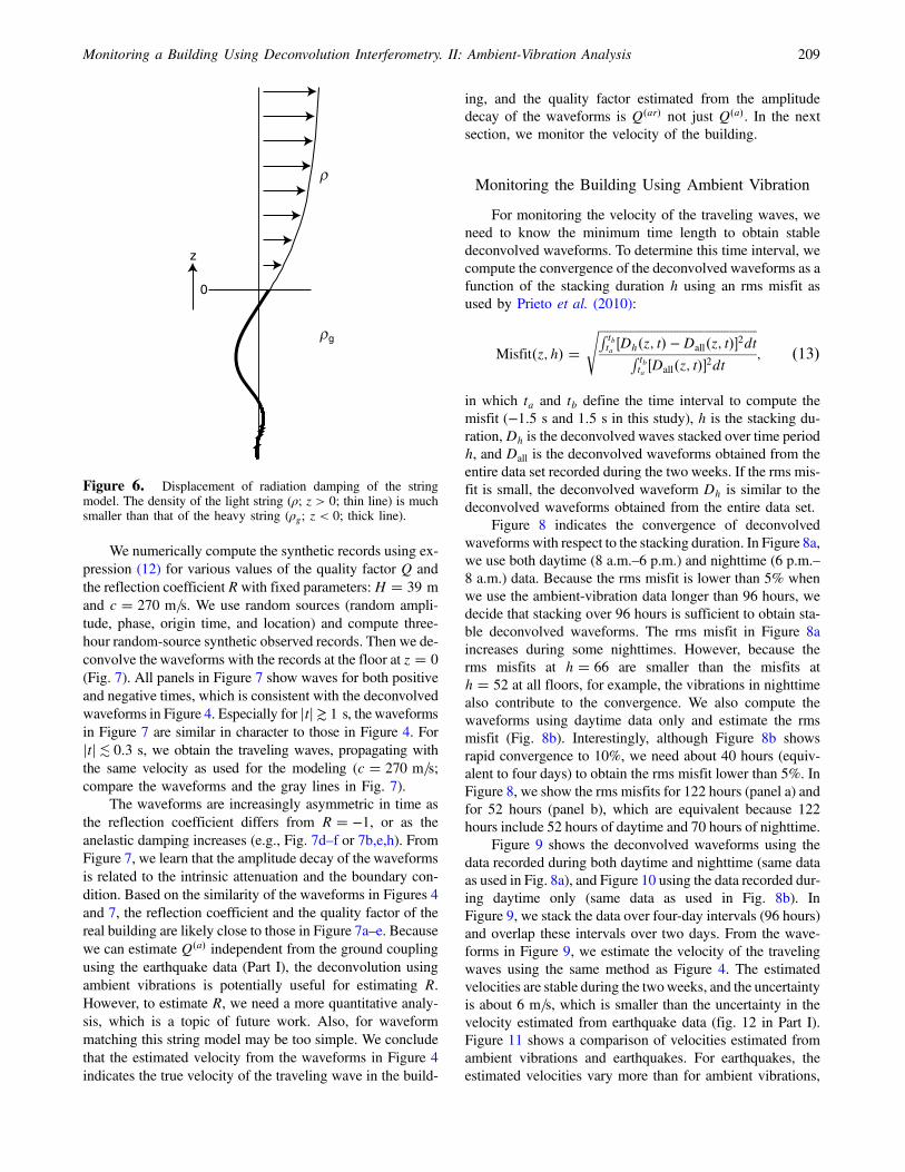
The model for our normal-mode analysis is a 1D stringmodel that includes radiation damping (Snieder, 2004a,chapter 20.10). This model consists of an open-ended lightstring with mass density ρ connected to a heavy string withdensity ρg ≫ ρ at z � 0 (Fig. 6). The wave propagation inthe light and heavy strings represents the propagation in thebuilding and the subsurface, respectively. Although the stringmodel is primitive, the model qualitatively accounts for thewave propagation in the building because of three reasons;(1) we are only interested in the building, (2) the effect of theground for the building is limited to the coupling at z � 0,and (3) we assume no waves return after the waves propagateto the ground. The ratio of the densities of the light and heavystrings is related to the reflection coefficient at the connectionof the strings (at the base of the building) (Coulson andJeffrey, 1977, chapter 2):

R ����ρ

p − �����ρg

p���ρ

p � �����ρg

p � −1� ϵ

1� ϵ; �6�

in which

ϵ �����������ρ=ρg

q: �7�

We carry out a perturbation analysis for this smalldimensionless parameter.

The eigenfunctions and eigenfrequencies of this stringmodel to first order in ϵ for the mode m (m � 0; 1; )are given by

um�z� � sin���m� 1

2

�πzH

�

− iϵH − zH

cos���m� 1

2

�πzH

�; �8�

and

ω�r�m �

���m� 1

2

�π − iϵ

�cH; �9�

respectively (see Appendix). Because this string model doesnot include the intrinsic attenuation of the building, the ei-genfrequency in expression (9) does not incorporate the at-tenuation. The superscript in expression (9) indicates that thecomplex eigenfrequency accounts only for the radiation loss.Snieder and Şafak (2006) derive the eigenfrequency (ω�a�

m )with the intrinsic attenuation, but without radiation damping:

ω�a�m �

�m� 1

2

�πcH

��1 − iγ�: �10�

Comparing expressions (9) and (10), we account for the in-trinsic attenuation and the radiation damping using theeigenfrequency

ω�ar�m �

�π

�m� 1

2

���1 − iγ� − iϵ

�cH; �11�

for which we assume the intrinsic attenuation to be weakand ignore a cross term between the intrinsic attenuationand radiation damping. In expression (11), the first term,π�m� 1=2�c=H, is the frequency in case there is no intrinsicattenuation (γ � 0) and the building has a rigid boundary atthe bottom (R � −1). The second term, −iγπ�m� 1=2�c=H,accounts for the intrinsic attenuation, and the third term,−iϵc=H, accounts for the radiation loss at the base of thebuilding. The waveforms in this string model with the intrin-sic attenuation are given by the summation of normal modes(Snieder, 2004a):

u�z;ω� �X∞m�0

um�z�Ru�m�z′�F�z′�dz′

�ω�ar�m �2 − ω2

; �12�

in which F indicates the forces that excite the vibrations.

0

9

18

27

36

(a) (b)

−0.5 0 0.5 1Time (s)

Ele

vatio

n (m

)

−0.5 0 0.5 1Time (s)

Figure 5. (a) Synthetic waveforms obtained from one source inside a building (expressions 2 and 3) and (b) waveforms of panel (a) afterdeconvolution with the waves observed at z � 0 m. The source is located at zs � 13 m and excites waves at t � 0:2 s. The gray lines in panel(b) show the arrival times of the traveling waves based on expressions (4) and (5). The solid and dashed gray lines illustrate the termseik�z−2zs�e−γjkj�z−2zs� and Reikze−γjkjz, respectively, and their reverberations. The amplitudes of panels (a) and (b) are normalized after applyingthe same band-pass filter as used in Figure 4.

208 N. Nakata and R. Snieder

We numerically compute the synthetic records using ex-pression (12) for various values of the quality factor Q andthe reflection coefficient R with fixed parameters:H � 39 mand c � 270 m=s. We use random sources (random ampli-tude, phase, origin time, and location) and compute three-hour random-source synthetic observed records. Then we de-convolve the waveforms with the records at the floor at z � 0

(Fig. 7). All panels in Figure 7 show waves for both positiveand negative times, which is consistent with the deconvolvedwaveforms in Figure 4. Especially for jtj ≳ 1 s, the waveformsin Figure 7 are similar in character to those in Figure 4. Forjtj≲ 0:3 s, we obtain the traveling waves, propagating withthe same velocity as used for the modeling (c � 270 m=s;compare the waveforms and the gray lines in Fig. 7).

The waveforms are increasingly asymmetric in time asthe reflection coefficient differs from R � −1, or as theanelastic damping increases (e.g., Fig. 7d–f or 7b,e,h). FromFigure 7, we learn that the amplitude decay of the waveformsis related to the intrinsic attenuation and the boundary con-dition. Based on the similarity of the waveforms in Figures 4and 7, the reflection coefficient and the quality factor of thereal building are likely close to those in Figure 7a–e. Becausewe can estimate Q�a� independent from the ground couplingusing the earthquake data (Part I), the deconvolution usingambient vibrations is potentially useful for estimating R.However, to estimate R, we need a more quantitative analy-sis, which is a topic of future work. Also, for waveformmatching this string model may be too simple. We concludethat the estimated velocity from the waveforms in Figure 4indicates the true velocity of the traveling wave in the build-

ing, and the quality factor estimated from the amplitudedecay of the waveforms is Q�ar� not just Q�a�. In the nextsection, we monitor the velocity of the building.

Monitoring the Building Using Ambient Vibration

For monitoring the velocity of the traveling waves, weneed to know the minimum time length to obtain stabledeconvolved waveforms. To determine this time interval, wecompute the convergence of the deconvolved waveforms as afunction of the stacking duration h using an rms misfit asused by Prieto et al. (2010):

Misfit�z; h� �������������������������������������������������������R tbta �Dh�z; t� −Dall�z; t��2dtR tb

ta �Dall�z; t��2dt

s; �13�

in which ta and tb define the time interval to compute themisfit (−1:5 s and 1:5 s in this study), h is the stacking du-ration,Dh is the deconvolved waves stacked over time periodh, and Dall is the deconvolved waveforms obtained from theentire data set recorded during the two weeks. If the rms mis-fit is small, the deconvolved waveform Dh is similar to thedeconvolved waveforms obtained from the entire data set.

Figure 8 indicates the convergence of deconvolvedwaveforms with respect to the stacking duration. In Figure 8a,we use both daytime (8 a.m.–6 p.m.) and nighttime (6 p.m.–8 a.m.) data. Because the rms misfit is lower than 5% whenwe use the ambient-vibration data longer than 96 hours, wedecide that stacking over 96 hours is sufficient to obtain sta-ble deconvolved waveforms. The rms misfit in Figure 8aincreases during some nighttimes. However, because therms misfits at h � 66 are smaller than the misfits ath � 52 at all floors, for example, the vibrations in nighttimealso contribute to the convergence. We also compute thewaveforms using daytime data only and estimate the rmsmisfit (Fig. 8b). Interestingly, although Figure 8b showsrapid convergence to 10%, we need about 40 hours (equiv-alent to four days) to obtain the rms misfit lower than 5%. InFigure 8, we show the rms misfits for 122 hours (panel a) andfor 52 hours (panel b), which are equivalent because 122hours include 52 hours of daytime and 70 hours of nighttime.

Figure 9 shows the deconvolved waveforms using thedata recorded during both daytime and nighttime (same dataas used in Fig. 8a), and Figure 10 using the data recorded dur-ing daytime only (same data as used in Fig. 8b). InFigure 9, we stack the data over four-day intervals (96 hours)and overlap these intervals over two days. From the wave-forms in Figure 9, we estimate the velocity of the travelingwaves using the same method as Figure 4. The estimatedvelocities are stable during the twoweeks, and the uncertaintyis about 6 m=s, which is smaller than the uncertainty in thevelocity estimated from earthquake data (fig. 12 in Part I).Figure 11 shows a comparison of velocities estimated fromambient vibrations and earthquakes. For earthquakes, theestimated velocities vary more than for ambient vibrations,

z

0

ρ

ρg

Figure 6. Displacement of radiation damping of the stringmodel. The density of the light string (ρ; z > 0; thin line) is muchsmaller than that of the heavy string (ρg; z < 0; thick line).

Monitoring a Building Using Deconvolution Interferometry. II: Ambient-Vibration Analysis 209

and the acceleration of the observed records also varies(fig. 12b in Part I). These variations indicate that the velocitiesestimated from earthquakes include nonlinear effects. Thevelocities estimated from ambient vibrations are not affectedby nonlinearity because the acceleration of the observed re-

cords is small and does not vary much. Therefore, ambientvibration is appropriate for monitoring the velocity of travel-ing waves in the linear regime. Deconvolved waveforms inFigure 10 are similar to those in Figure 9, and the differencesin estimated velocities are not statistically significant.

0

15

30

−1.5 −1 −0.5 0 0.5 1 1.5

Time (s)

Ele

vatio

n (m

)

Q=5, R=−1

−1 −0.5 0 0.5 1 1.5

Time (s)

Q=5, R=−0.9

−1 −0.5 0 0.5 1 1.5

Time (s)

Q=5, R=−0.8

0

15

30

Ele

vatio

n (m

)

Q=20, R=−1 Q=20, R=−0.9 Q=20, R=−0.8

0

15

30

(a) (b) (c)

(d) (e) (f)

(g) (h) (i)

Ele

vatio

n (m

)

Q=100, R=−1 Q=100, R=−0.9 Q=100, R=−0.8

Figure 7. Synthetic deconvolved waveforms using three hour random vibrations as sources after applying the same band-pass filter as inFigure 4. Panels (a)–(i) are computed by adopting different quality factorsQ and reflection coefficients R (see lower left of each panel). Graylines indicate the arrival time of the traveling wave with the velocity used for the modeling (c � 270 m=s). The scale of the amplitudes at eachpanel is the same.

0 20 40 60 80 100 1200

5

10

15

20

25

30

35

Stacking duration (h)

rms

mis

fit (

%)

248

0 10 20 30 40 500

5

10

15

20

25

30

35

Stacking duration (h)

rms

mis

fit (

%)

(b)(a)248

Figure 8. Convergence test of ambient-vibration interferometry based on rms misfits (equation 13) as a function of the stacking duration.(a) The rms misfits with respect to the stacked waveform over two-week ambient vibrations, recorded in both daytime (8 a.m.–6 p.m.) andnighttime (6 p.m.–8 a.m.). The shaded areas correspond to night times. We show the misfits at the second, fourth, and eighth floors. (b) Therms misfits with respect to the same waveforms as panel (a), but using only daytime data. We show the rms misfits for 122 hours (52 hours ofdaytime and 70 hours of nighttime) in panel (a) and 52 hours in panel (b).

210 N. Nakata and R. Snieder

Conclusions

We retrieve traveling waves inside the building byapplying seismic interferometry to ambient-vibration data.In contrast to the case in which sources are only outsidethe building (i.e., earthquakes), deconvolved waves obtainedfrom ambient vibrations are nonzero for both positive andnegative times, which is explained because multiple sourcessimultaneously excite inside the building. Based on the nor-mal-mode analysis, we synthetically reconstruct waveformsthat are qualitatively similar to the real data using the simplestring model. The velocity estimated from the syntheticwaveforms with this model is the same as the true velocityalthough the attenuation estimated from the decay of the am-plitude with time is not equal to the intrinsic attenuation ofthe building. Because the amplitude decay is also influencedby radiation losses at the base of the building, we are, in prin-ciple, able to estimate both quality factors and reflection co-efficients separately from the amplitude of the waveforms,which requires a more accurate model than the string modelused here. For monitoring the building, we find the time in-terval to obtain stable waveforms using the convergence test,and we need deconvolved ambient vibrations averaged overfour days to obtain stable waveforms for this building. Thevelocity estimated from ambient-vibration data is morestable than that from earthquake data because the ambientvibrations are due to the linear response of the building.

Data and Resources

Seismograms used in this study were operated andmaintained by Suncoh Consultants Co., Ltd. Figure 1 was

produced using Generic Mapping Tools (GMT; available athttp://gmt.soest.hawaii.edu, last accessed June 2013).

Acknowledgments

We want to thank Suncoh Consultant Co., Ltd. and Akebono BrakeIndustry Co., Ltd. for providing the data. We thank Seiichiro Kuroda forhis professional comments to improve this work. N.N. thanks the instructorand classmates of the class Academic Publishing in Colorado School ofMines for their help in preparing this manuscript. This work was supported

5/31−6/4

6/2−6/6

6/4−6/8

6/6−6/10

6/8−6/12

6/10−6/14

(a) (b)

−1 0 1

Dat

e

Time (s)

260 270 280

Velocity (m/s)

Figure 9. (a) Time-lapse deconvolved waveforms averagedover 96 hours with a 48 hour overlap using ambient vibrations re-corded in both daytime and nighttime. We have applied the sameband-pass filter as used in Figure 4. (b) Shear-wave velocities esti-mated from the traveling waves in panel (a). The width of each boxindicates one standard deviation of estimated velocities at eachfloor.

5/31−6/4

6/2−6/6

6/4−6/8

6/6−6/10

6/8−6/12

6/10−6/14(a) (b)

−1 0 1

Dat

e

Time (s)260 270 280

Velocity (m/s)

Figure 10. (a) Time-lapse deconvolved waveforms averagedover 40 hours, with a 20 hour overlap using ambient vibration re-corded in daytime only. We have applied the same band-pass filteras used in Figure 4. (b) Shear-wave velocities estimated from thetraveling waves in panel (a). The width of each box indicates onestandard deviation of estimated velocities at each floor.

1 2 3 4 5 6 7 8 9 10 11 12 13 14200

220

240

260

280

Date (June 2011)

Vel

ocity

(m

/s)

Ambient vibrationEarthquake

Figure 11. Velocities estimated from ambient vibrations re-corded in both daytime and nighttime (black) and earthquakes usinga stretching method in Part I (gray). The labels of the date are placedat the start of days (midnight). The velocities in black are plotted atthe center of each 96 hour interval and those in the gray are at theorigin time of each earthquake. The error bars correspond to the barsshown in figures 9 and 12 in Part I, respectively.

Monitoring a Building Using Deconvolution Interferometry. II: Ambient-Vibration Analysis 211

by the Consortium Project on Seismic Inverse Methods for ComplexStructures at the Center for Wave Phenomena.

References

Aki, K. (1957). Space and time spectra of stationary stochastic waves,with special reference to microtremors, Bull. Earthq. Res. Inst. 35,415–456.

Aki, K., and P. G. Richards (2002). Quantitative Seismology, 2nd Ed., Univ.Science Books, Sausalito, California, 700 pp.

Bakulin, A., and R. Calvert (2006). The virtual source method: Theory andcase study, Geophysics 71, no. 4, S1139–S1150.

Bensen, G. D., M. H. Ritzwoller, M. P. Barmin, A. L. Levshin, F. Lin,M. P. Moschetti, N. M. Shapiro, and Y. Yang (2007). Processing seis-mic ambient noise data to obtain reliable broad-band surface wavedispersion measurements, Geophys. J. Int. 169, 1239–1260.

Brenguier, F., M. Campillo, C. Hadziioannou, N. M. Shapiro, R. M. Nadeau,and E. Larose (2008). Postseismic relaxation along the San AndreasFault at Parkfield from continuous seismological observations, Science321, 1478–1481.

Brenguier, F., N. M. Shapiro, M. Campllo, V. Ferrazzini, Z. Duputel,O. Coutant, and A. Nercessian (2008). Towards forecasting volcaniceruptions using seismic noise, Nature Geosci. 1, 126–130.

Claerbout, J. F. (1968). Synthesis of a layered medium from its acoustictransmission response, Geophysics 33, no. 2, 264–269.

Clayton, R. W., and R. A. Wiggins (1976). Source shape estimation anddeconvolution of teleseismic bodywaves, Geophys. J. Roy. Astron.Soc. 47, 151–177.

Clinton, J. F., S. C. Bradford, T. H. Heaton, and J. Favela (2006). Theobserved wander of the natural frequencies in a structure, Bull.Seismol. Soc. Am. 96, no. 1, 237–257.

Coulson, C. A., and A. Jeffrey (1977).Waves: A Mathematical Approach tothe Common Types of Wave Motion, 2nd Ed., Longman, United King-dom, 240 pp.

Dahlen, F. A., and J. Tromp (1998). Theoretical Global Seismology, Prince-ton University Press, Princeton, New Jersey, 944 pp.

Derode, A., E. Larose, M. Tanter, J. de Rosny, A. Tourin, M. Campillo, andM. Fink (2003). Recovering the Green’s function from field-fieldcorrelations in an open scattering medium (L), J. Acoust. Soc. Am.113, no. 6, 2973–2976.

Draganov, D., X. Campman, J. Thorbecke, A. Verdel, and K. Wapenaar(2009). Reflection images from ambient seismic noise, Geophysics74, no. 5, A63–A67.

Ivanović, S. S., M. D. Trifunac, and M. I. Todorovska (2000). Ambientvibration tests of structures—A review, ISET J. Earthq. Tech. 37,no. 4, 165–197.

Kanai, K., and S. Yoshizawa (1961). On the period and the damping ofvibration in actual buildings, Bull. Earthq. Res. Inst. 39, 477–489.

Kohler, M. D., T. H. Heaton, and S. C. Bradford (2007). Propagating wavesin the steel, moment-frame Factor building recorded during earth-quakes, Bull. Seismol. Soc. Am. 97, no. 4, 1334–1345.

Lobkis, O. I., and R. L. Weaver (2001). On the emergence of the Green’sfunction in the correlations of a diffuse field, J. Acoust. Soc. Am. 110,no. 6, 3011–3017.

Mehta, K., J. L. Sheiman, R. Snieder, and R. Calvert (2008). Strengtheningthe virtual-source method for time-lapse monitoring, Geophysics 73,no. 3, S73–S80.

Michel, C., P. Guéguen, and P.-Y. Bard (2008). Dynamic parameters ofstructures extracted from ambient vibration measurements: An aidfor the seismic vulnerability assessment of existing buildings inmoderate seismic hazard regions, Soil Dynam. Earthq. Eng. 28,593–604.

Miyazawa, M., R. Snieder, and A. Venkataraman (2008). Application ofseismic interferometry to extract P- and S-wave propagation andobservation of shear-wave splitting from noise data at Cold Lake,Alberta, Canada, Geophysics 73, no. 4, D35–D40.

Nakata, N., and R. Snieder (2011). Near-surface weakening in Japan afterthe 2011 Tohoku-Oki earthquake,Geophys. Res. Lett. 38, L17302, doi:10.1029/2011GL048800.

Nakata, N., and R. Snieder (2012a). Estimating near-surface shear-wavevelocities in Japan by applying seismic interferometry to KiK-net data,J. Geophys. Res. 117, no. B01308, doi: 10.1029/2011JB008595.

Nakata, N., and R. Snieder (2012b). Time-lapse change in anisotropy inJapan’s near surface after the 2011 Tohoku-Oki earthquake, Geophys.Res. Lett. 39, L11313, doi: 10.1029/2012GL051979.

Nakata, N., R. Snieder, S. Kuroda, S. Ito, T. Aizawa, and T. Kunimi (2013).Monitoring a building using deconvolution interferometry, I:Earthquake-data analysis, Bull. Seismol. Soc. Am. 103, no. 3, 1662–1678, doi: 10.1785/0120120291.

Nakata, N., R. Snieder, T. Tsuji, K. Larner, and T. Matsuoka (2011).Shear-wave imaging from traffic noise using seismic interferometryby cross-coherence, Geophysics 76, no. 6, SA97–SA106, doi:10.1190/GEO2010-0188.1.

Prieto, G. A., J. F. Lawrence, A. I. Chung, and M. D. Kohler (2010). Impulseresponse of civil structures from ambient noise analysis, Bull. Seismol.Soc. Am. 100, no. 5A, 2322–2328.

Sawazaki, K., H. Sato, H. Nakahara, and T. Nishimura (2009). Time-lapsechanges of seismic velocity in the shallow ground caused by strongground motion shock of the 2000 western-Tottori earthquake, Japan,as revealed from coda deconvolution analysis, Bull. Seismol. Soc. Am.99, no. 1, 352–366.

Schuster, G. (2009). Seismic Interferometry, Cambridge Univ. Press, NewYork, 260 pp.

Sens-Schönfelder, C., and U. Wegler (2006). Passive image interferometryand seasonal variations of seismic velocities at Merapi Volcano,Indonesia, Geophys. Res. Lett. 33, L21302, doi: 10.1029/2006GL027797.

Snieder, R. (2004a). A Guided Tour of Mathematical Methods for thePhysical Sciences, Cambridge Univ. Press, United Kingdom, 507 pp.

Snieder, R. (2004b). Extracting the Green’s function from the correlation ofcoda waves: A derivation based on stationary phase, Phys. Rev. E 69,046,610.

Snieder, R., and E. Şafak (2006). Extracting the building response usingseismic interferometry: Theory and application to the Millikan Libraryin Pasadena, California, Bull. Seismol. Soc. Am. 96, no. 2, 586–598.

Snieder, R., M. Miyazawa, E. Slob, I. Vasconcelos, and K.Wapenaar (2009).A comparison of strategies for seismic interferometry, Surv. Geophys.30, no. 10, 503–523.

Snieder, R., J. Sheiman, and R. Calvert (2006). Equivalence of the virtual-source method and wave-field deconvolution in seismic interferom-etry, Phys. Rev. E 73, 066,620.

Todorovska, M. I., and M. D. Trifunac (2008a). Earthquake damage detec-tion in the Imperial Country Services Building III: Analysis of wavetravel times via impulse response functions, Soil Dynam. Earthq. Eng.28, 387–404.

Todorovska, M. I., andM. D. Trifunac (2008b). Impulse response analysis ofthe Van Nuys 7-story hotel during 11 earthquakes and earthquakedamage detection, Struct. Control Health Monit. 15, 90–116.

Trifunac, M. D. (1972). Comparisons between ambient and forced vibrationexperiments, Earthq. Eng. Struct. Dynam. 1, 133–150.

Trifunac, M. D., S. S. Ivanović, and M. I. Todorovska (2001a). Apparentperiods of a building. I: Fourier analysis, J. Struct. Eng. 127, no. 5,517–526.

Trifunac, M. D., S. S. Ivanović, and M. I. Todorovska (2001b). Apparentperiods of a building. II: Time-frequency analysis, J. Struct. Eng.127, no. 5, 527–537.

Tsai, V. C. (2011). Understanding the amplitudes of noise correlationmeasurements, J. Geophys. Res. 116, no. B09311, doi: 10.1029/2011JB008483.

van der Neut, J., J. Thorbecke, K. Mehta, E. Slob, and K. Wapenaar (2011).Controlled-source interferometric redatuming by crosscorrelation andmultidimensional deconvolution in elastic media, Geophysics 76,no. 4, SA63–SA76, doi: 10.1190/1.3580633.

212 N. Nakata and R. Snieder

Vasconcelos, I., and R. Snieder (2008a). Interferometry by deconvolution,Part 1—Theory for acoustic waves and numerical examples, Geophys-ics 73, no. 3, S115–S128.

Vasconcelos, I., and R. Snieder (2008b). Interferometry by deconvolution:Part 2—Theory for elastic waves and application to drill-bit seismicimaging, Geophysics 73, no. 3, S129–S141.

Wapenaar, K. (2004). Retrieving the elastodynamic Green’s function of anarbitrary inhomogeneous medium by cross correlation, Phys. Rev. Lett.93, 254–301.

Wegler, U., and C. Sens-Schönfelder (2007). Fault zone monitoring withpassive image interferometry, Geophys. J. Int. 168, 1029–1033.

Wegler, U., B.-G. Lühr, R. Snieder, and A. Ratdomopurbo (2006).Increase of shear wave velocity before the 1998 eruption of Merapivolcano (Indonesia), Geophys. J. Int. 33, L09303, doi: 10.1029/2006GL025928.

Yamada, M., J. Mori, and S. Ohmi (2010). Temporal changes of subsurfacevelocities during strong shaking as seen from seismic interferometry,J. Geophys. Res. 115, B03,302.

Appendix

Eigenfunctions and Eigenfrequenciesof the String Model

In this appendix, we derive the eigenfunctions (expres-sion 8) and eigenfrequencies (expression 9) of the stringmodel (Fig. 6) using a perturbation analysis in the smallparameter ϵ (expression 7). The normal modes of the unper-turbed string (ϵ � 0, ρg � ∞, and R � −1) are given by

u�z > 0� � sin k�u�z; �A1�

u�z < 0� � 0; �A2�in which k�u� is the unperturbed wavenumber. The parameterϵ accounts for the coupling of the light string to the heavystring (expression 6). For the unperturbed model (ϵ � 0), thestring has infinite mass for z < 0, and hence it does notmove. When ϵ ≠ 0, the waveforms, which include perturbedwaves, are expressed by

u�z > 0� � sin kz� A cos kz; �A3�

u�z < 0� � Be−ikgz; �A4�

respectively. The coefficients A and B depend on ϵ. Accord-ing to expression (A4), waves are radiated downward in thelower (heavy) part of the string (the thick line in Fig. 6). Theratio of the wavenumbers in the light and heavy strings(k=kg) is given by chapter 2 in Coulson and Jeffrey (1977):

k=kg � ϵ: �A5�

The boundary conditions of the model are ∂u=∂z � 0 atz � H, and u and ∂u=∂z are continuous at z � 0. From

expressions (A3) and (A4) and these boundary conditions,we obtain

kkgsinkH� icoskH� ϵ

2i

�eikH−e−ikH

� i2

�eikH�e−ikH

�0; �A6�

in which we use expression (A5) for k=kg. From expres-sion (A6), we obtain

e2ikH � −1 − ϵ

1� ϵ: �A7�

Applying a first-order Taylor expansion in ϵ to the wave-number in expression (A7), we obtain the wavenumber formode m:

km ����m� 1

2

�π − iϵ

�1

H; �A8�

in which the real and imaginary of km are the unperturbedand perturbed parts of the wavenumber of mode m,respectively. The perturbation of the wavenumber causedby the radiation damping (−iϵ=H) is constant for all modes.The eigenfrequency ωm that corresponds to the wavenumberin expression (A8) is given by expression (9).

From expressions (A3) and (A8), the waveform (eigen-function) for the mode m within the light string is given by

um�z� � sin�kmz� � A cos�kmz�

� sin�kmz� �cos�kmH�sin�kmH� cos�kmz�

� cosfkm�H − z�gsin�kmH� ; �A9�

in which we use the boundary condition ∂u=∂z � 0 atz � H at the second equality. Using Taylor expansions tofirst order in ϵ in the sine and cosine functions, we derive theeigenfunction shown in expression (8).

Department of GeophysicsStanford University397 Panama MallStanford, California 94305nnakata@stanford.edu

(N.N.)

Center for Wave PhenomenaDepartment of GeophysicsColorado School of Mines1500 Illinois StreetGolden, Colorado 80401rsnieder@mines.edu

(R.S.)

Manuscript received 23 February 2013;Published Online 26 November 2013

Monitoring a Building Using Deconvolution Interferometry. II: Ambient-Vibration Analysis 213