tutorial on seismic interferometry: part 1 — basic...

TP

K

pafscpoapf

©

lI

G1

EOPHYSICS, VOL. 75, NO. 5 �SEPTEMBER-OCTOBER 2010�; P. 75A195–75A209, 15 FIGS.0.1190/1.3457445

utorial on seismic interferometry:art 1 — Basic principles and applications

ees Wapenaar1, Deyan Draganov1, Roel Snieder2, Xander Campman3, and Arie Verdel3

raweItretimonaswt

ABSTRACT

Seismic interferometry involves the crosscorrelation of re-sponses at different receivers to obtain the Green’s function be-tween these receivers. For the simple situation of an impulsiveplane wave propagating along the x-axis, the crosscorrelation ofthe responses at two receivers along the x-axis gives the Green’sfunction of the direct wave between these receivers. When thesource function of the plane wave is a transient �as in explorationseismology� or a noise signal �as in passive seismology�, then thecrosscorrelation gives the Green’s function, convolved with theautocorrelation of the source function. Direct-wave interferome-try also holds for 2D and 3D situations, assuming the receiversare surrounded by a uniform distribution of sources. In this case,the main contributions to the retrieved direct wave between thereceivers come from sources in Fresnel zones around stationarypoints. The main application of direct-wave interferometry is the

siessSpDnps

Septeme Netheo, U.S.s. E-ma

ers to thmic inteate. Wh

75A195

Downloaded 15 Sep 2010 to 138.67.20.77. Redistribution subject to S

etrieval of seismic surface-wave responses from ambient noisend the subsequent tomographic determination of the surface-ave velocity distribution of the subsurface. Seismic interferom-

try is not restricted to retrieving direct waves between receivers.n a classic paper, Claerbout shows that the autocorrelation of theransmission response of a layered medium gives the plane-waveeflection response of that medium. This is essentially 1D reflect-d-wave interferometry. Similarly, the crosscorrelation of theransmission responses, observed at two receivers, of an arbitrarynhomogeneous medium gives the 3D reflection response of that

edium. One of the main applications of reflected-wave interfer-metry is retrieving the seismic reflection response from ambientoise and imaging of the reflectors in the subsurface. A commonspect of direct- and reflected-wave interferometry is that virtualources are created at positions where there are only receiversithout requiring knowledge of the subsurface medium parame-

ers or of the positions of the actual sources.

INTRODUCTION

In this two-part tutorial, we give an overview of the basic princi-les and the underlying theory of seismic interferometry and discusspplications and new advances. The term seismic interferometry re-ers to the principle of generating new seismic responses of virtualources4 by crosscorrelating seismic observations at different re-eiver locations. One can distinguish between controlled-source andassive seismic interferometry. Controlled-source seismic interfer-metry, pioneered by Schuster �2001�, Bakulin and Calvert �2004�,nd others, comprises a new processing methodology for seismic ex-loration data. Apart from crosscorrelation, controlled-source inter-erometry also involves summation of correlations over different

Manuscript received by the Editor 30 November 2009; published online 141Delft University of Technology, Department of Geotechnology, Delft, Th2Colorado School of Mines, Center for Wave Phenomena, Golden, Colorad3Shell International Exploration and Production, Rijswijk, The Netherland2010 Society of Exploration Geophysicists.All rights reserved.4In the literature on seismic interferometry, the term virtual source often ref

y in Part 2. However, creating a virtual source is the essence of nearly all seisn this paper �Parts 1 and 2� we use the term virtual source whenever appropri

ource positions. Passive seismic interferometry, on the other hand,s a methodology for turning passive seismic measurements �ambi-nt seismic noise or microearthquake responses� into deterministiceismic responses. Here, we further distinguish between retrievingurface-wave transmission responses �Campillo and Paul, 2003;hapiro and Campillo, 2004; Sabra, Gerstoft, et al., 2005a� and ex-loration reflection responses �Claerbout, 1968; Scherbaum, 1987b;raganov et al., 2007, 2009�. In passive interferometry of ambientoise, no explicit summation of correlations over different sourceositions is required because the correlated responses are a superpo-ition of simultaneously acting uncorrelated sources.

In all cases, the response that is retrieved by crosscorrelating two

ber 2010.rlands. E-mail: [email protected]; [email protected]. E-mail: [email protected]: [email protected]; [email protected].

e method of Bakulin and Calvert �2004, 2006�, which is discussed extensive-rferometry methods �see e.g., Schuster �2001�, who already used this term�.

en it refers to Bakulin and Calvert’s method, we will mention this explicitly.

EG license or copyright; see Terms of Use at http://segdl.org/

rtcpatelsws�Wp

cLimHnmGTtGtR

toctcoaht

otpwcoits

1

asaWuFdftsaGfSt

aphct�

atxtxxlwabw

cGtc�

i�

tdh

FwsaciG

75A196 Wapenaar et al.

eceiver recordings �and summing over different sources� can be in-erpreted as the response that would be measured at one of the re-eiver locations as if there were a source at the other. Because such aoint-source response is equal to a Green’s function convolved withwavelet, seismic interferometry is also often called Green’s func-

ion retrieval. Both terms are used in this paper. The term interferom-try is borrowed from radio astronomy, where it refers to crosscorre-ation methods applied to radio signals from distant objects �Thomp-on et al., 2001�. The name Green’s function honors George Greenho, in a privately published essay, introduced the use of impulse re-

ponses in field representations �Green, 1828�. Challis and Sheard2003� give a brief history of Green’s life and theorem. Ramírez and

eglein �2009� review applications of Green’s theorem in seismicrocessing.

Early successful results of Green’s function retrieval from noiseorrelations were obtained in the field of ultrasonics �Weaver andobkis, 2001, 2002�. The experiments were done with diffuse fields

n a closed system. Here diffuse means that the amplitudes of the nor-al modes are uncorrelated but have equal expected energies.ence, the crosscorrelation of the field at two receiver positions doesot contain cross-terms of unequal normal modes. The sum of the re-aining terms is proportional to the modal representation of thereen’s function of the closed system �Lobkis and Weaver, 2001�.his means that the crosscorrelation of a diffuse field in a closed sys-

em converges to its impulse response. Later, it was recognized �e.g.,odin, 2007� that this theoretical explanation is akin to the fluctua-

ion-dissipation theorem �Callen and Welton, 1951; Rytov, 1956;ytov et al., 1989; Le Bellac et al., 2004�.The earth is a closed system; but at the scale of global seismology,

he wavefield is far from diffuse.At the scale of exploration seismol-gy, an ambient-noise field may have a diffuse character, but the en-ompassing system is not closed. Hence, for seismic interferometry,he normal-mode approach breaks down. Throughout this paper, weonsider seismic interferometry �or Green’s function retrieval� inpen systems, including half-spaces below a free surface. Instead oftreatment per field of application or a chronological discussion, weave chosen a setup in which we explain the principles of seismic in-erferometry step by step. In Part 1, we start with the basic principles

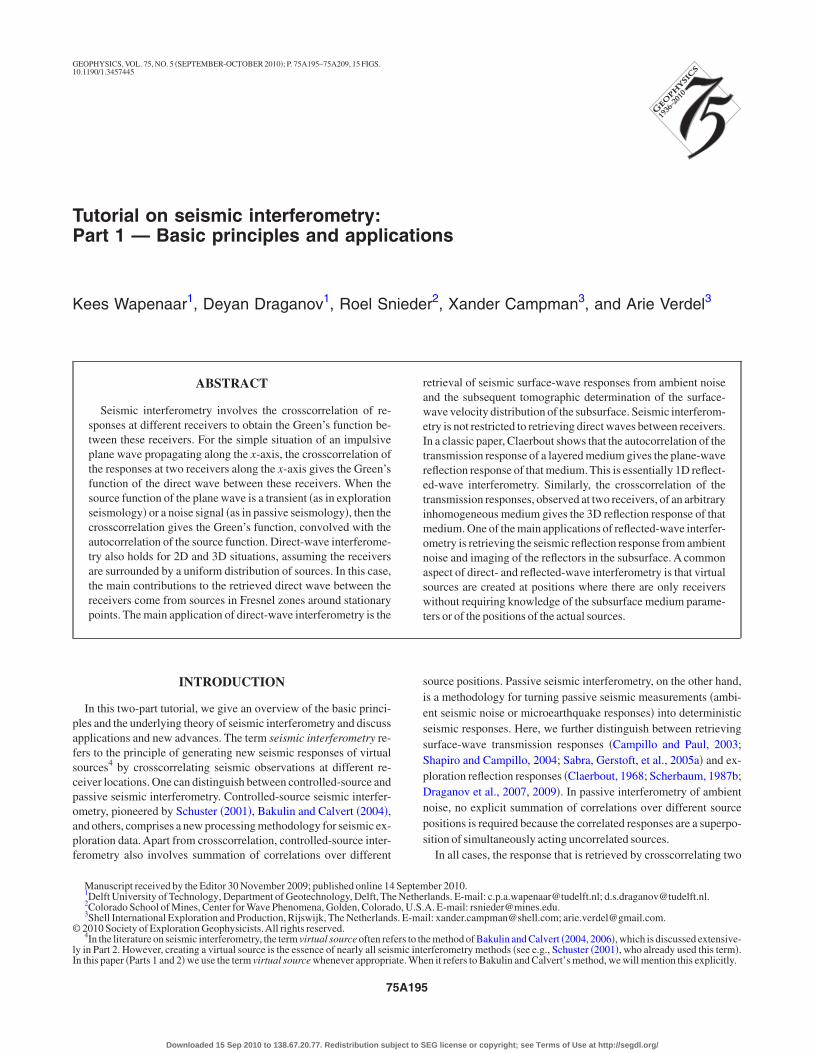
igure 1. A 1D example of direct-wave interferometry. �a� A planeave traveling rightward along the x-axis, emitted by an impulsive

ource at x�xS and t�0. �b� The response observed by a receivert xA. This is the Green’s function G�xA,xS,t�. �c�As in �b� but for a re-eiver at xB. �d� Crosscorrelation of the responses at xA and xB. This isnterpreted as the response of a source at xA, observed at xB, i.e.,�x ,x ,t�.
B A

f 1D direct-wave interferometry and conclude with a discussion ofhe principles of 3D reflected-wave interferometry. We present ap-lications in controlled-source as well as passive interferometry and,here appropriate, review the historical background. To stay fo-

used on seismic applications, we refrain from a further discussionf the normal-mode approach, nor do we address the many interest-ng applications of Green’s function retrieval in underwater acous-ics �e.g., Roux and Fink, 2003; Sabra et al., 2005; Brooks and Ger-toft, 2007�.

DIRECT-WAVE INTERFEROMETRY

D analysis of direct-wave interferometry

We start our explanation of seismic interferometry by consideringn illustrative 1D analysis of direct-wave interferometry. Figure 1ahows a plane wave, radiated by an impulsive unit source at x�xS

nd t�0, propagating in the rightward direction along the x-axis.e assume that the propagation velocity c is constant and the medi-

m is lossless. There are two receivers along the x-axis at xA and xB.igure 1b shows the response observed by the first receiver at xA. Weenote this response as G�xA,xS,t�, where G stands for the Green’sunction. Throughout this paper, we use the common conventionhat the first two arguments in G�xA,xS,t� denote the receiver andource coordinates, respectively �here, xA and xS�, whereas the lastrgument denotes time t or angular frequency �. In our example, thisreen’s function consists of an impulse at tA� �xA�xS� /c; there-

ore, G�xA,xS,t�� t� tA�, where � �t� is the Dirac delta function.imilarly, the response at xB is given by G�xB,xS,t�� t� tB�, with

B� �xB�xS� /c �Figure 1c�.Seismic interferometry involves the crosscorrelation of responses

t two receivers, in this case at xA and xB. Looking at Figure 1a, it ap-ears that the raypaths associated with G�xA,xS,t� and G�xB,xS,t�ave the path from xS to xA in common. The traveltime along thisommon path cancels in the crosscorrelation process, leaving theraveltime along the remaining path from xA to xB, i.e., tB� tA� �xB

xA� /c. Hence, the crosscorrelation of the responses in Figure 1bnd c is an impulse at tB� tA �see Figure 1d�. This impulse can be in-erpreted as the response of a source at xA observed by a receiver at

B, i.e., the Green’s function G�xB,xA,t�.An interesting observation ishat the propagation velocity c and the position of the actual source

S need not be known. The traveltimes along the common path from

S to xA compensate each other, independent of the propagation ve-ocity and the length of this path. Similarly, if the source impulseould occur at t� tS instead of at t�0, the impulses observed at xA

nd xB would be shifted by the same amount of time tS, which woulde canceled in the crosscorrelation. Thus, the absolute time tS athich the source emits its pulse need not be known.Let us discuss this example a bit more precisely. We denote the

rosscorrelation of the impulse responses at xA and xB as�xB,xS,t��G�xA,xS,�t�. The asterisk denotes temporal convolu-

ion, but the time reversal of the second Green’s function turns theonvolution into a correlation, defined as G�xB,xS,t��G�xA,xS,�t�

�G�xB,xS,t� t��G�xA,xS,t��dt�. Substituting the delta functionsnto the right-hand side gives �� t� t�� tB�� t�� tA�dt�� t

�tB� tA�� t� �xB�xA� /c�. This is indeed the Green’s func-ion G�xB,xA,t�, propagating from xA to xB. Because we started thiserivation with the crosscorrelation of the Green’s functions, weave obtained the following 1D Green’s function representation:


Too�G

fx�

tuvc

ItGc

FbnI1tsass

tnvffitfb�to

ptaxt��G3

W

w

Wsb�Gctr

FTAen

Fst

Tutorial on interferometry: Part 1 75A197

G�xB,xA,t��G�xB,xS,t��G�xA,xS,� t� . �1�

his representation formulates the principle that the crosscorrelationf observations at two receivers �xA and xB� gives the response at onef those receivers �xB� as if there were a source at the other receiverxA�. It also shows why seismic interferometry is often calledreen’s function retrieval.Note that the source is not necessarily an impulse. If the source

unction is defined by some wavelet s�t�, then the responses at xA and

B can be written as u�xA,xS,t��G�xA,xS,t��s�t� and u�xB,xS,t�G�xB,xS,t��s�t�, respectively. Let Ss�t� be the autocorrelation of

he wavelet, i.e., Ss�t��s�t��s��t�. Then the crosscorrelation of�xA,xS,t� and u�xB,xS,t� gives the right-hand side of equation 1, con-olved with Ss�t�. This is equal to the left-hand side of equation 1,onvolved with Ss�t�. Therefore,

G�xB,xA,t��Ss�t��u�xB,xS,t��u�xA,xS,� t� . �2�

n words: If the source function is a wavelet instead of an impulse,hen the crosscorrelation of the responses at two receivers gives thereen’s function between these receivers, convolved with the auto-

orrelation of the source function.This principle holds true for any source function, including noise.

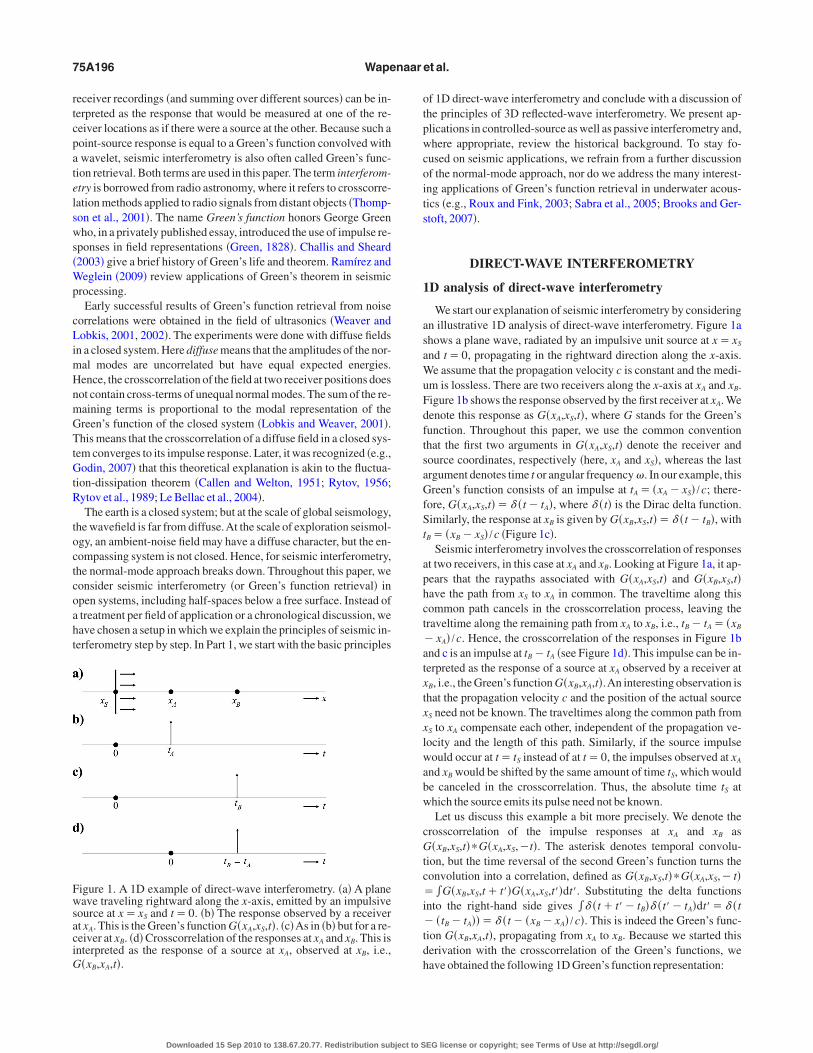
igure 2a and b shows the responses at xA and xB, respectively, of aandlimited noise source N�t� at xS �the central frequency of theoise is 30 Hz; the figure shows only 4 s of a total of 160 s of noise�.n this numerical example, the distance between the receivers is200 m and the propagation velocity is 2000 m /s; hence, the travel-ime between these receivers is 0.6 s.As a consequence, the noise re-ponse at xB in Figure 2b is 0.6 s delayed with respect to the responset xA in Figure 2a �similar to the impulse in Figure 1c delayed with re-pect to the impulse in Figure 1b�. Crosscorrelation of these noise re-ponses gives, analogous to equation 2, the impulse response be-

igure 2. As in Figure 1 but this time for a noise source N�t� at xS. �a�he response observed at xA, i.e., u�xA,xS,t��G�xA,xS,t��N�t�. �b�s in �a� but for a receiver at xB. �c� The crosscorrelation, which is

qual to G�xB,xA,t��SN�t�, with SN�t� the autocorrelation of theoise.


ween xA and xB, convolved with SN�t�, i.e., the autocorrelation of theoise N�t�. The correlation is shown in Figure 2c, which indeed re-eals a bandlimited impulse centered at t�0.6 s �the traveltimerom xA to xB�. Note that from registrations at two receivers of a noiseeld from an unknown source in a medium with unknown propaga-

ion velocity, we have obtained a bandlimited version of the Green’sunction. By dividing the distance between the receivers �1200 m�y the traveltime estimated from the bandlimited Green’s function0.6 s�, we obtain an estimate of the propagation velocity betweenhe receivers �2000 m /s�. This illustrates that direct-wave interfer-metry can be used for tomographic inversion.

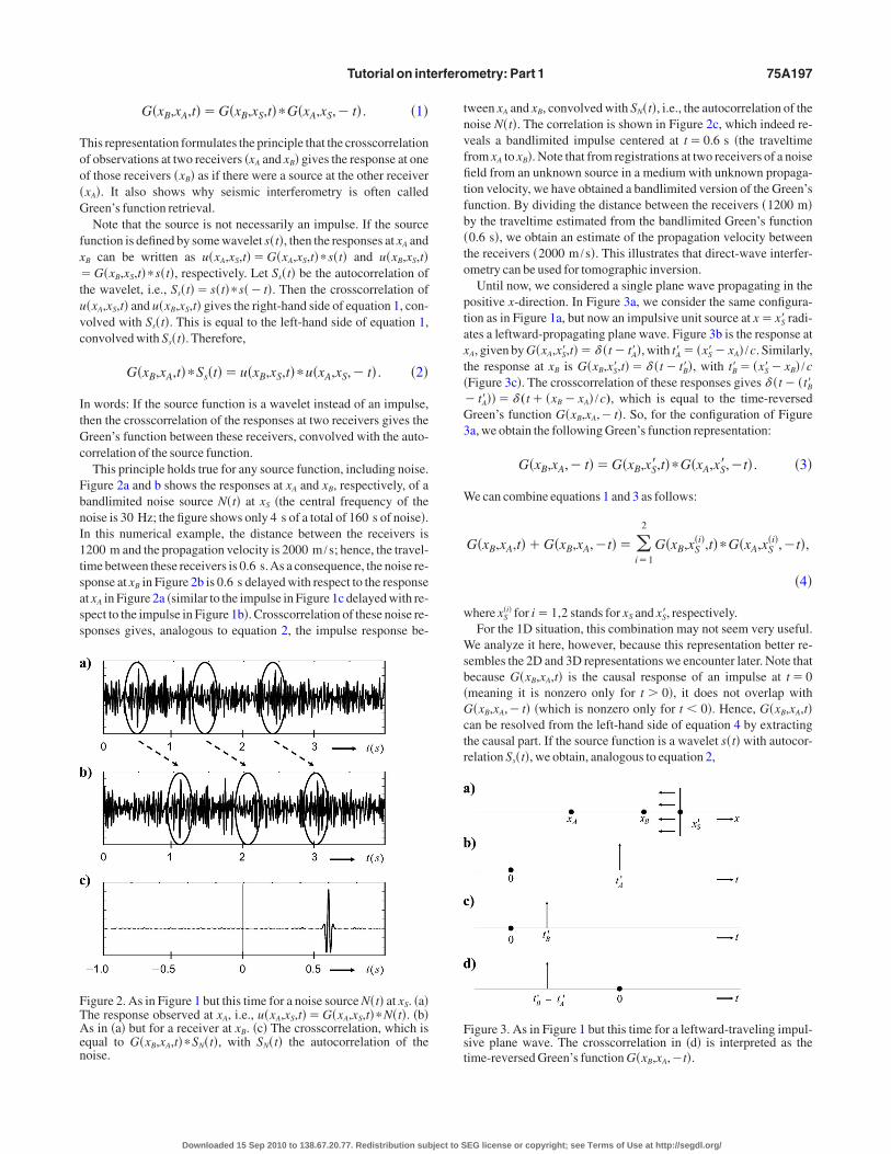
Until now, we considered a single plane wave propagating in theositive x-direction. In Figure 3a, we consider the same configura-ion as in Figure 1a, but now an impulsive unit source at x�xS� radi-tes a leftward-propagating plane wave. Figure 3b is the response atA, given by G�xA,xS�,t�� t� tA��, with tA� � �xS��xA� /c. Similarly,he response at xB is G�xB,xS�,t�� t� tB��, with tB� � �xS��xB� /cFigure 3c�. The crosscorrelation of these responses gives � �t� �tB�

tA�� (t� �xB�xA� /c), which is equal to the time-reversedreen’s function G�xB,xA,�t�. So, for the configuration of Figurea, we obtain the following Green’s function representation:

G�xB,xA,� t��G�xB,xS�,t��G�xA,xS�,�t� . �3�

e can combine equations 1 and 3 as follows:

G�xB,xA,t��G�xB,xA,�t�� i�1

2

G�xB,xS�i�,t��G�xA,xS

�i�,�t�,

�4�

here xS�i� for i�1,2 stands for xS and xS�, respectively.

For the 1D situation, this combination may not seem very useful.e analyze it here, however, because this representation better re-

embles the 2D and 3D representations we encounter later. Note thatecause G�xB,xA,t� is the causal response of an impulse at t�0meaning it is nonzero only for t � 0�, it does not overlap with�xB,xA,�t� �which is nonzero only for t � 0�. Hence, G�xB,xA,t�

an be resolved from the left-hand side of equation 4 by extractinghe causal part. If the source function is a wavelet s�t� with autocor-elation Ss�t�, we obtain, analogous to equation 2,

igure 3. As in Figure 1 but this time for a leftward-traveling impul-ive plane wave. The crosscorrelation in �d� is interpreted as theime-reversed Green’s function G�x ,x ,�t�.
B A

H�

tf�

lwsctbuuttis

tt�

stt�s�iot5c

C

Eawxr4u

dLmGitw

itc

Fai

Fat


�G�xB,xA,t��G�xB,xA,� t��Ss�t�

� �i�1

2

u�xB,xS�i�,t��u�xA,xS

�i�,� t� . �5�

ere, G�xB,xA,t��Ss�t� may have some overlap with G�xB,xA,t��Ss�t� for small �t�, depending on the length of the autocorrela-

ion function Ss�t�. Therefore, G�xB,xA,t��Ss�t� can be extractedrom the left-hand side of equation 5, except for small distances �xB

xA�.The right-hand sides of equations 4 and 5 state that the crosscorre-

ation is applied to the responses of each source separately, afterhich the summation over the sources is carried out. For impulsive

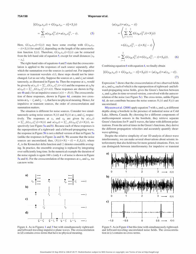
ources or transient wavelets s�t�, these steps should not be inter-hanged. Let us see why. Suppose the sources at xS and xS� act simul-aneously, as illustrated in Figure 4a. Then the response at xA woulde given by u�xA,t��i�1

2 G�xA,xS�i�,t��s�t� and the response at xB by

�xB,t�� j�12 G�xB,xS

�j�,t��s�t�. These responses are shown in Fig-re 4b and c for an impulsive source �s�t�� t��. The crosscorrela-ion of these responses, shown in Figure 4d, contains two cross-erms at tB� tA� and tB� � tA that have no physical meaning. Hence, formpulsive or transient sources, the order of crosscorrelation andummation matters.

The situation is different for noise sources. Consider two simul-aneously acting noise sources N1�t� and N2�t� at xS and xS�, respec-ively. The responses at xA and xB are given by u�xA,t�

�i�12 G�xA,xS

�i�,t��Ni�t� and u�xB,t�� j�12 G�xB,xS

�j�,t��Nj�t�, re-pectively �see Figure 5a and b�. Because each of these responses ishe superposition of a rightward- and a leftward-propagating wave,he response in Figure 5b is not a shifted version of that in Figure 5aunlike the responses in Figure 2a and b�. We assume that the noiseources are uncorrelated; thus, �Nj�t��Ni��t�� ijSN�t�, where

ij is the Kronecker delta function and �·� denotes ensemble averag-ng. In practice, the ensemble averaging is replaced by integratingver sufficiently long time. In the numerical example the duration ofhe noise signals is again 160 s �only 4 s of noise is shown in Figurea and b�. For the crosscorrelation of the responses at xA and xB, wean now write

igure 4. As in Figures 1 and 3 but with simultaneously rightward-nd leftward-traveling impulsive plane waves. The crosscorrelationn �d� contains cross-terms that have no physical meaning.


�u�xB,t��u�xA,� t�

��j�1

2

�i�1

2

G�xB,xS�j�,t��Nj�t�

�G�xA,xS�i�,� t��Ni�� t��

� �i�1

2

G�xB,xS�i�,t��G�xA,xS

�i�,� t��SN�t� . �6�

ombining equation 6 with equation 4, we finally obtain

�G�xB,xA,t��G�xB,xA,� t��SN�t�� u�xB,t��u�xA,�t� .

�7�

xpression 7 shows that the crosscorrelation of two observed fieldst xA and xB, each of which is the superposition of rightward- and left-ard-propagating noise fields, gives the Green’s function between

A and xB plus its time-reversed version, convolved with the autocor-elation of the noise �see Figure 5c�. The cross-terms, unlike Figured, do not contribute because the noise sources N1�t� and N2�t� arencorrelated.

Miyazawa et al. �2008� apply equation 7 with xA and xB at differentepths along a borehole in the presence of industrial noise at Coldake, Alberta, Canada. By choosing for u different components ofulticomponent sensors in the borehole, they retrieve separatereen’s functions for P- and S-waves, the latter with different polar-

zations. From the arrival times in the Green’s functions, they derivehe different propagation velocities and accurately quantify shear-ave splitting.Despite the relative simplicity of our 1D analysis of direct-wave

nterferometry, we can make several observations about seismic in-erferometry that also hold true for more general situations. First, wean distinguish between interferometry for impulsive or transient

igure 5. As in Figure 4 but this time with simultaneously rightward-nd leftward-traveling uncorrelated noise fields. The crosscorrela-ion in �c� contains no cross-terms.


snorpl

r�ilmr

stsaNGs�d

2i

fshes�

61ac2bhbectitrsstpseaSNv

tlm

pl�rae

00 s.


ources on the one hand �equations 4 and 5� and interferometry foroise sources on the other hand �equation 7�. In the case of impulsiver transient sources, the responses of each source must be crosscor-elated separately, after which a summation over the sources takeslace. In the case of uncorrelated noise sources, a single crosscorre-ation suffices.

Second, it appears that an isotropic illumination of the receivers isequired to obtain a time-symmetric response between the receiversof which the causal part is the actual response�. In one dimension,sotropic illumination means equal illumination by rightward- andeftward-propagating waves. In two and three di-

ensions, it means equal illumination from all di-ections �discussed in the next section�.

Finally, instead of the time-symmetric re-ponse G�xB,xA,t��G�xB,xA,�t�, in the litera-ure we often encounter an antisymmetric re-ponse G�xB,xA,t��G�xB,xA,�t�. This is merelyresult of differently defined Green’s functions.ote that a simple time differentiation of thereen’s functions would turn the symmetric re-

ponse into an antisymmetric one, and vice versasee Wapenaar and Fokkema �2006� for a moreetailed discussion on this aspect�.

D and 3D analysis of direct-waventerferometry

We extend our discussion of direct-wave inter-erometry to configurations with more dimen-ions. In the following discussion, we mainly useeuristic arguments, illustrated with a numericalxample. For a more precise derivation based ontationary-phase analysis, we refer to Snieder2004�.

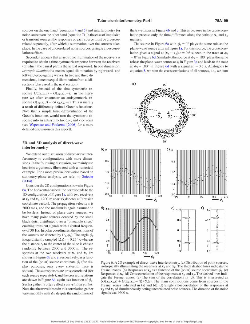
Consider the 2D configuration shown in Figurea. The horizontal dashed line corresponds to theD configuration of Figure 1a, with two receiverst xA and xB, 1200 m apart �x denotes a Cartesianoordinate vector�. The propagation velocity c is000 m /s, and the medium is again assumed toe lossless. Instead of plane-wave sources, weave many point sources denoted by the smalllack dots, distributed over a “pineapple slice,”mitting transient signals with a central frequen-y of 30 Hz. In polar coordinates, the positions ofhe sources are denoted by �rS,�S�. The angle �S

s equidistantly sampled ��S�0.25° �, whereashe distance rS to the center of the slice is chosenandomly between 2000 and 3000 m. The re-ponses at the two receivers at xA and xB arehown in Figure 6b and c, respectively, as a func-ion of the �polar� source coordinate �S �for dis-lay purposes, only every sixteenth trace ishown�. These responses are crosscorrelated �forach source separately�, and the crosscorrelationsre shown in Figure 6d, again as a function of �S.uch a gather is often called a correlation gather.ote that the traveltimes in this correlation gatherary smoothly with �S, despite the randomness of

Figure 6. A 2Disotropically iFresnel zonesResponses at xcate the Fresn�G�xB,xA,t��Fresnel zonesxA and xB of sisignals was 96


he traveltimes in Figure 6b and c. This is because in the crosscorre-ation process only the time difference along the paths to xA and xB

atters.The source in Figure 6a with �S�0° plays the same role as the

lane-wave source at xS in Figure 1a. For this source, the crosscorre-ation gives a signal at �xB�xA� /c�0.6 s, seen in the trace at �S

0° in Figure 6d. Similarly, the source at �S�180° plays the sameole as the plane-wave source at xS� in Figure 3a and leads to the tracet �S�180° in Figure 6d with a signal at �0.6 s. Analogous toquation 5, we sum the crosscorrelations of all sources, i.e., we sum

ple of direct-wave interferometry. �a� Distribution of point sources,ating the receivers at xA and xB. The thick dashed lines indicate theesponses at xA as a function of the �polar� source coordinate �S. �c�

rosscorrelation of the responses at xA and xB. The dashed lines indi-es. �e� The sum of the correlations in �d�. This is interpreted asxA,�t��Ss�t�. The main contributions come from sources in theted in �a� and �d�. �f� Single crosscorrelation of the responses ateously acting uncorrelated noise sources. The duration of the noise

examllumin. �b� R

B. �d� Cel zonG�xB,indica

multan


aiap�BsbFdpedntn

tpnnn�tsofiSW

sst

ssgbssGufstscG

otwp�ewtaptsoambb

Fsrtt


ll traces in Figure 6d, which leads to the time-symmetric responsen Figure 6e, with two events at 0.6 and �0.6 s. These two eventsre again interpreted as the response of a source at xA, observed at xB,lus its time-reversed version, i.e., �G�xB,xA,t��G�xB,xA,

t��Ss�t�, where Ss�t� is the autocorrelation of the source wavelet.ecause the sources have a finite frequency content, not only do the

ources exactly at �S�0° and �S�180° contribute to these eventsut also the sources in Fresnel zones around these angles. Theseresnel zones are denoted by the thick dashed lines in Figure 6a and. In Figure 6d, the centers of these Fresnel zones are the stationaryoints of the traveltime curve of the crosscorrelations. Note that thevents in all traces outside the Fresnel zones in Figure 6d interfereestructively and give no coherent contribution in Figure 6e. Theoise between the two events in Figure 6e results because the travel-ime curve in Figure 6d is not 100% smooth, caused by the random-ess of the source positions in Figure 6a.

The response in Figure 6e is obtained by summing crosscorrela-ions of independent transient sources. Using the arguments in therevious section, we can replace the transient sources with simulta-eously acting noise sources. The cross-terms disappear when theoise sources are uncorrelated; hence, a single crosscorrelation ofoise observations at xA and xB gives, analogous to equation 7,G�xB,xA,t��G�xB,xA,�t��SN�t�, where SN�t� is the autocorrela-ion of the noise �see Figure 6f�. Note that the symmetry of the re-ponses in Figure 6e and f relies again on the isotropic illuminationf the receivers, i.e., on the net power flux of the illuminating wave-eld being �close to� zero �van Tiggelen, 2003; Malcolm et al., 2004;ánchez-Sesma et al., 2006; Snieder et al., 2007; Perton et al., 2009;eaver et al., 2009; Yao et al., 2009�.Of course, what is demonstrated here for a 2D distribution of

ources also holds for a 3D source distribution. In that case, allources in Fresnel volumes rather than Fresnel zones contribute tohe retrieval of the direct wave between xA and xB. Furthermore, the

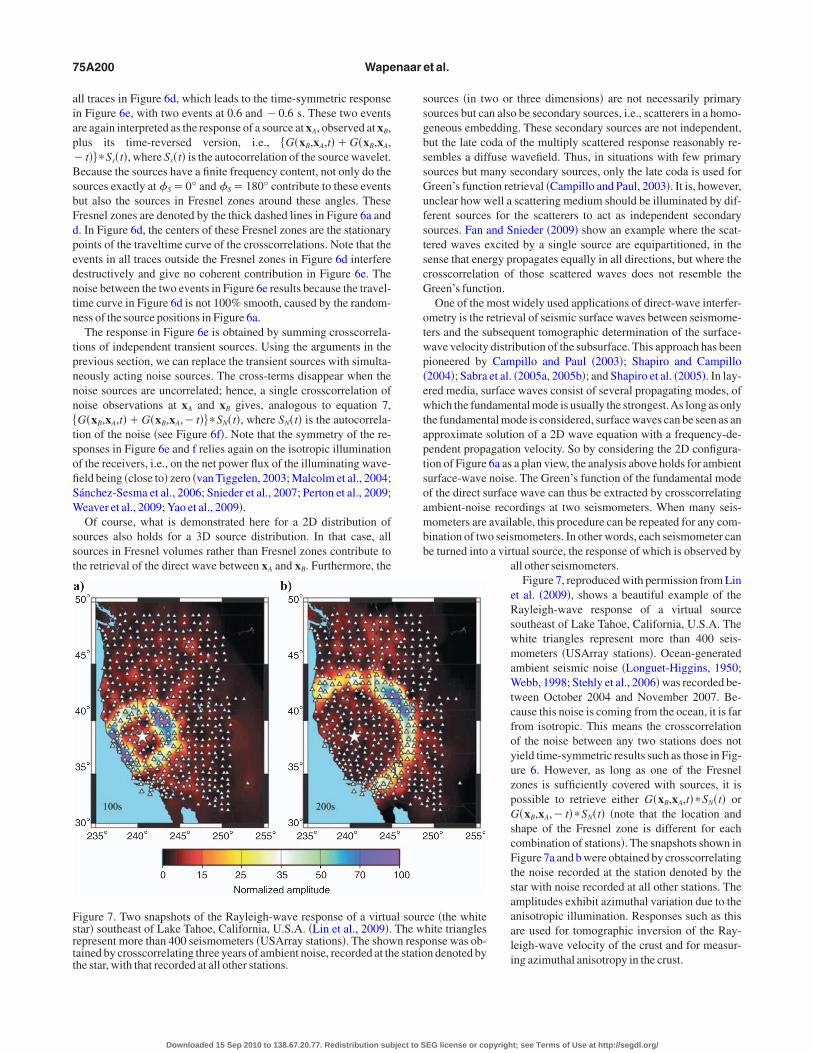
igure 7. Two snapshots of the Rayleigh-wave response of a virtutar� southeast of Lake Tahoe, California, U.S.A. �Lin et al., 2009�.epresent more than 400 seismometers �USArray stations�. The showained by crosscorrelating three years of ambient noise, recorded at thhe star, with that recorded at all other stations.


ources �in two or three dimensions� are not necessarily primaryources but can also be secondary sources, i.e., scatterers in a homo-eneous embedding. These secondary sources are not independent,ut the late coda of the multiply scattered response reasonably re-embles a diffuse wavefield. Thus, in situations with few primaryources but many secondary sources, only the late coda is used forreen’s function retrieval �Campillo and Paul, 2003�. It is, however,nclear how well a scattering medium should be illuminated by dif-erent sources for the scatterers to act as independent secondaryources. Fan and Snieder �2009� show an example where the scat-ered waves excited by a single source are equipartitioned, in theense that energy propagates equally in all directions, but where therosscorrelation of those scattered waves does not resemble thereen’s function.One of the most widely used applications of direct-wave interfer-

metry is the retrieval of seismic surface waves between seismome-ers and the subsequent tomographic determination of the surface-ave velocity distribution of the subsurface. This approach has beenioneered by Campillo and Paul �2003�; Shapiro and Campillo2004�; Sabra et al. �2005a, 2005b�; and Shapiro et al. �2005�. In lay-red media, surface waves consist of several propagating modes, ofhich the fundamental mode is usually the strongest.As long as only

he fundamental mode is considered, surface waves can be seen as anpproximate solution of a 2D wave equation with a frequency-de-endent propagation velocity. So by considering the 2D configura-ion of Figure 6a as a plan view, the analysis above holds for ambienturface-wave noise. The Green’s function of the fundamental modef the direct surface wave can thus be extracted by crosscorrelatingmbient-noise recordings at two seismometers. When many seis-ometers are available, this procedure can be repeated for any com-

ination of two seismometers. In other words, each seismometer cane turned into a virtual source, the response of which is observed by

all other seismometers.Figure 7, reproduced with permission from Lin

et al. �2009�, shows a beautiful example of theRayleigh-wave response of a virtual sourcesoutheast of Lake Tahoe, California, U.S.A. Thewhite triangles represent more than 400 seis-mometers �USArray stations�. Ocean-generatedambient seismic noise �Longuet-Higgins, 1950;Webb, 1998; Stehly et al., 2006� was recorded be-tween October 2004 and November 2007. Be-cause this noise is coming from the ocean, it is farfrom isotropic. This means the crosscorrelationof the noise between any two stations does notyield time-symmetric results such as those in Fig-ure 6. However, as long as one of the Fresnelzones is sufficiently covered with sources, it ispossible to retrieve either G�xB,xA,t��SN�t� orG�xB,xA,�t��SN�t� �note that the location andshape of the Fresnel zone is different for eachcombination of stations�. The snapshots shown inFigure 7a and b were obtained by crosscorrelatingthe noise recorded at the station denoted by thestar with noise recorded at all other stations. Theamplitudes exhibit azimuthal variation due to theanisotropic illumination. Responses such as thisare used for tomographic inversion of the Ray-leigh-wave velocity of the crust and for measur-ing azimuthal anisotropy in the crust.

ce �the whitehite trianglesonse was ob-n denoted by

al sourThe wn resp

e statio


l�FhfmasLLd�ctsfl

etrFwccqdtaiemadt

1

epsetrtel1acbiHsr

el

lers��eutfttsnc��

rrs�Tst�c

Tr

w2fa

F2wratfi


Bensen et al. �2007� show that it is possible to retrieve the Ray-eigh-wave velocity as a function of frequency. Brenguier et al.2007� combine these approaches to 3D tomographic inversion.rom noise measurements at the Piton de la Fournaise volcano, theyave retrieved the Rayleigh-wave group velocity distribution as aunction of frequency and used this to derive a 3D S-wave velocityodel of the interior of the volcano. In the past couple of years, the

pplications of direct surface-wave interferometry have expandedpectacularly. Without any claim of completeness, we mentionarose et al. �2005�, Gerstoft et al. �2006�, Kang and Shin �2006�,arose et al. �2006�, Yao et al. �2006�, Bensen et al. �2008�, Goué-ard et al. �2008a, 2008b�, Liang and Langston �2008�, Lin et al.2008�, Ma et al. �2008�, Yao et al. �2008�, Li et al. �2009�, and Pi-ozzi et al. �2009�. The success of these applications is explained byhe fact that surface waves are by far the strongest events in ambienteismic noise. In the next section, we show that the retrieval of re-ected waves from ambient seismic noise is an order more difficult.Direct surface-wave interferometry has an interesting link with

arly work by Aki �1957, 1965� and Toksöz �1964� on the spatial au-ocorrelation �SPAC� method. The SPAC method uses a circular ar-ay of seismometers plus a seismometer at the center of the circle.or a distribution of uncorrelated fundamental-mode Rayleighaves propagating as plane waves in all directions, the spatial auto-

orrelation function obtained from the circular array reveals the lo-al surface-wave velocity as a function of frequency and, subse-uently, the local depth-dependent velocity profile. An importantifference with the interferometry approach is that the distances be-ween the receivers in the SPAC method are usually smaller than halfwavelength �Henstridge, 1979�, making it a local method; whereas

n direct-wave interferometry, the distances are assumed much larg-r than the wavelength because otherwise the stationary-phase argu-ents would not hold. More recent discussions on the SPAC method

re given by Okada �2003, 2006� and Asten �2006�. An interestingiscussion on the relation between the SPAC method and seismic in-erferometry is given by Yokoi and Margaryan �2008�.

REFLECTED-WAVE INTERFEROMETRY

D analysis of reflected-wave interferometry

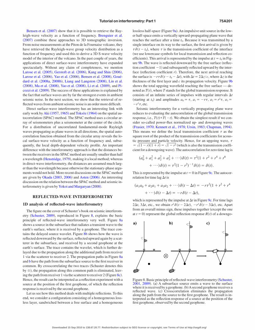
The figure on the cover of Schuster’s book on seismic interferom-try �Schuster, 2009�, reproduced in Figure 8, explains the basicrinciple of reflected-wave interferometry very well. Figure 8ahows a source in the subsurface that radiates a transient wave to thearth’s surface, where it is received by a geophone. The trace con-ains the delayed source wavelet. Figure 8b shows how the wave iseflected downward by the surface, reflected upward again by a scat-erer in the subsurface, and received by a second geophone at thearth’s surface. The trace contains the wavelet, which is further de-ayed due to the propagation along the additional path from receivervia the scatterer to receiver 2. The propagation paths in Figure 8a

nd b have the path from the subsurface source to the first receiver inommon. By crosscorrelating the two traces �Schuster denotes thisy ��, the propagation along this common path is eliminated, leav-ng the path from receiver 1 via the scatterer to receiver 2 �Figure 8c�.ence, the result can be interpreted as a reflection experiment with a

ource at the position of the first geophone, of which the reflectionesponse is received by the second geophone.

Let us see how this method deals with multiple reflections. To thisnd, we consider a configuration consisting of a homogeneous loss-ess layer, sandwiched between a free surface and a homogeneous


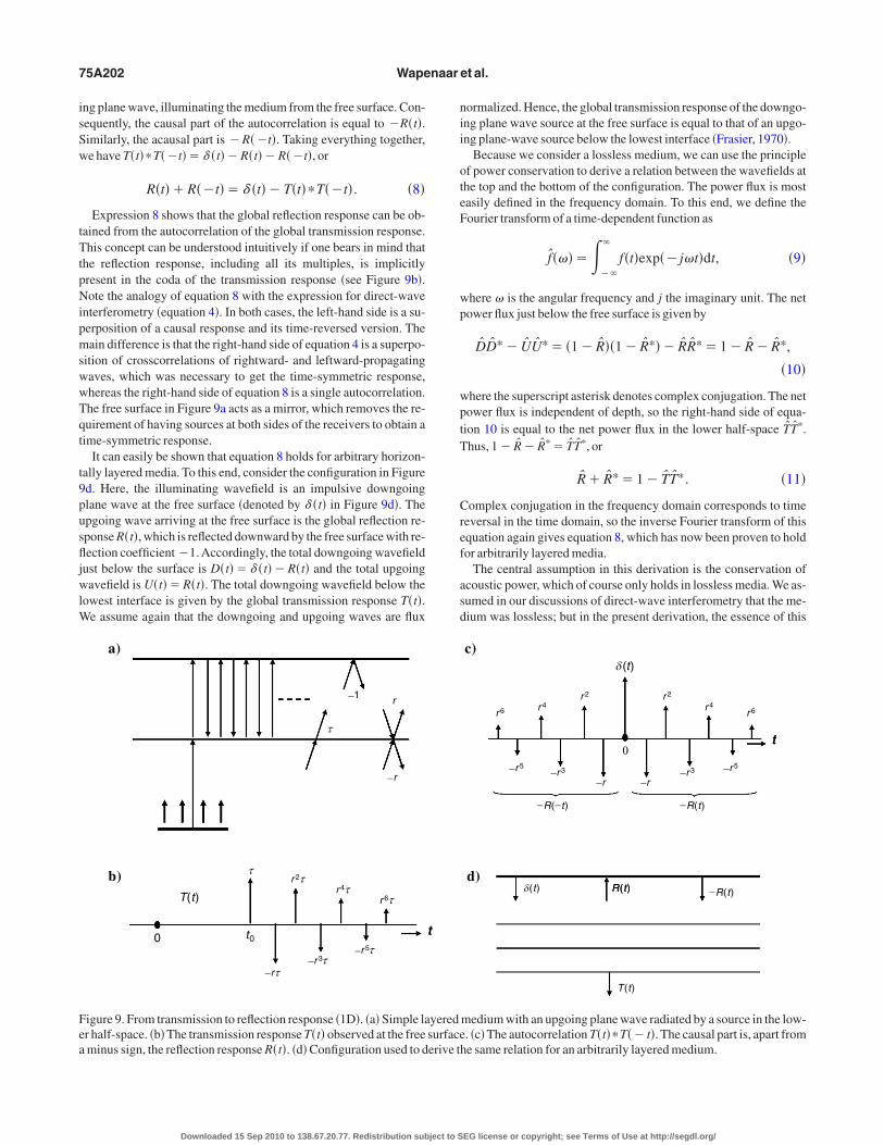
ossless half-space �Figure 9a�. An impulsive unit source in the low-r half-space emits a vertically upward-propagating plane wave thateaches the surface after a time t0. Because it was transmitted by aingle interface on its way to the surface, the first arrival is given by� �t� t0�, where � is the transmission coefficient of the interfacewe use lowercase symbols for local transmission and reflection co-fficients�. This arrival is represented by the impulse at t� t0 in Fig-re 9b. The wave is reflected downward by the free surface �reflec-ion coefficient �1� and subsequently reflected upward by the inter-ace �reflection coefficient r�. Therefore, the next arrival reachinghe surface is �r� � �t� t0��t�, with �t�2�z /c, where �z is thehickness of the first layer and c its propagation velocity. Figure 9bhows the total upgoing wavefield reaching the free surface — de-oted as T�t�, where T stands for the global transmission response. Itonsists of an infinite series of impulses with regular intervals �tstarting at t0� and amplitudes a0�� , a1��r� , a2�r2� , a3�

r3� , etc.Seismic interferometry for a vertically propagating plane wave

educes to evaluating the autocorrelation of the global transmissionesponse, i.e., T�t��T��t�. We obtain the simplest result if we con-ider so-called power-flux normalized up- and downgoing wavesFrasier, 1970; Kennett et al., 1978; Ursin, 1983; Chapman, 1994�.his means we define the local transmission coefficient � as thequare root of the product of the transmission coefficients for acous-ic pressure and particle velocity. Hence, for an upgoing wave, �

��1�r��1�r��1�r2 �which is also the transmission coeffi-ient for a downgoing wave�. The autocorrelation for zero time lag is

�a02�a1

2�a22�a3

2� ¯ �� t�� 2�1�r2�r4�r6

� ¯ �� t�� 2�1�r2��1� �t�� t� .

his is represented by the impulse at t�0 in Figure 9c. The autocor-elation for time lag �t is

�a1a0�a2a1�a3a2� ¯ �� t��t��r� 2�1�r2�r4

� ¯ �� t��t��r� �t��t�,

hich is represented by the impulse at �t in Figure 9c. For time lags�t, 3�t, etc., we obtain r2� �t�2�t�, �r3� �t�3�t�, etc. Apartrom an overall minus sign, these impulses together �except the onet t�0� represent the global reflection response R�t� of a downgo-

igure 8. Basic principle of reflected-wave interferometry �Schuster,001, 2009�. �a� A subsurface source emits a wave to the surfacehere it is received by a geophone. �b�Asecond geophone receives a

eflected wave. �c� Crosscorrelation eliminates the propagationlong the path from the source to the first geophone. The result is in-erpreted as the reflection response of a source at the position of therst geophone, observed by the second geophone.


isSw

tTtpNipmswwTqt

t9pusfljwlW

nii

oteF

wp

wptT

Cref

asd

Fea


ng plane wave, illuminating the medium from the free surface. Con-equently, the causal part of the autocorrelation is equal to �R�t�.imilarly, the acausal part is �R��t�. Taking everything together,e have T�t��T��t�� t��R�t��R��t�, or

R�t��R��t�� t��T�t��T��t� . �8�

Expression 8 shows that the global reflection response can be ob-ained from the autocorrelation of the global transmission response.his concept can be understood intuitively if one bears in mind that

he reflection response, including all its multiples, is implicitlyresent in the coda of the transmission response �see Figure 9b�.ote the analogy of equation 8 with the expression for direct-wave

nterferometry �equation 4�. In both cases, the left-hand side is a su-erposition of a causal response and its time-reversed version. Theain difference is that the right-hand side of equation 4 is a superpo-

ition of crosscorrelations of rightward- and leftward-propagatingaves, which was necessary to get the time-symmetric response,hereas the right-hand side of equation 8 is a single autocorrelation.he free surface in Figure 9a acts as a mirror, which removes the re-uirement of having sources at both sides of the receivers to obtain aime-symmetric response.

It can easily be shown that equation 8 holds for arbitrary horizon-ally layered media. To this end, consider the configuration in Figured. Here, the illuminating wavefield is an impulsive downgoinglane wave at the free surface �denoted by � �t� in Figure 9d�. Thepgoing wave arriving at the free surface is the global reflection re-ponse R�t�, which is reflected downward by the free surface with re-ection coefficient �1.Accordingly, the total downgoing wavefield

ust below the surface is D�t�� t��R�t� and the total upgoingavefield is U�t��R�t�. The total downgoing wavefield below the

owest interface is given by the global transmission response T�t�.e assume again that the downgoing and upgoing waves are flux

_1

_r

r

τ

a)

b)T(t)

r 2τ

τr 4τ

r 6τ

_r 5τ_r 3τ

_rτ

0 t0

igure 9. From transmission to reflection response �1D�. �a� Simple lar half-space. �b� The transmission response T�t� observed at the freeminus sign, the reflection response R�t�. �d� Configuration used to d


ormalized. Hence, the global transmission response of the downgo-ng plane wave source at the free surface is equal to that of an upgo-ng plane-wave source below the lowest interface �Frasier, 1970�.

Because we consider a lossless medium, we can use the principlef power conservation to derive a relation between the wavefields athe top and the bottom of the configuration. The power flux is mostasily defined in the frequency domain. To this end, we define theourier transform of a time-dependent function as

f��

�

f�t�exp��j�t�dt, �9�

here � is the angular frequency and j the imaginary unit. The netower flux just below the free surface is given by

DD*� UU*� �1� R��1� R*�� RR*�1� R� R*,

�10�

here the superscript asterisk denotes complex conjugation. The netower flux is independent of depth, so the right-hand side of equa-ion 10 is equal to the net power flux in the lower half-space TT*.hus, 1� R� R*� TT*, or

R� R*�1� TT*. �11�

omplex conjugation in the frequency domain corresponds to timeeversal in the time domain, so the inverse Fourier transform of thisquation again gives equation 8, which has now been proven to holdor arbitrarily layered media.

The central assumption in this derivation is the conservation ofcoustic power, which of course only holds in lossless media. We as-umed in our discussions of direct-wave interferometry that the me-ium was lossless; but in the present derivation, the essence of this

c)

r 6 r 4r 2 r 2

r 4r 6

_r 5 _r 3_r _r

_r 3_r 5

_R(_t) _R(t)

t

d)_R(t)R(t)R(t)δ(t)

T(t)

δ (t)

0

medium with an upgoing plane wave radiated by a source in the low-. �c� The autocorrelation T�t��T��t�. The causal part is, apart from

he same relation for an arbitrarily layered medium.

t

yeredsurfaceerive t


af2et

wUbaacbh

tusf

wtflabs3

e1n

2

cctC�tjmraas

sschaFp8btt

pwa

tlfipeipxacdstr

apcta

FetfloxxTr


ssumption has become manifest. Most approaches to seismic inter-erometry rely on the assumption that the medium is lossless. In Partof this tutorial, we also encounter approaches that account for loss-s or that use the essence of this assumption to estimate loss parame-ers.

We should note here that equation 8 for arbitrarily layered mediaas derived more than 40 years ago by Jon Claerbout at Stanfordniversity �Claerbout, 1968�. His expression looks slightly differentecause he did not use flux normalization. For his derivation, he usedrecursive method introduced by Thomson �1950�, Haskell �1953�,nd others. Later, he proposed the shorter derivation using energyonservation �Claerbout, 2000�. Frasier �1970� generalizes Claer-out’s result for obliquely propagating plane P- and SV-waves in aorizontally layered elastic medium.

Analogous to equations 5 and 7, equation 8 can be modified forransient or noise signals. For example, let u�t��T�t��N�t� be thepgoing wavefield at the surface, with N�t� representing the noiseignal emitted by the source in the lower half-space. Then we obtainrom equation 8

�R�t��R��t��SN�t��SN�t�� u�t��u��t�, �12�

here SN�t� is the autocorrelation of the noise. Equation 12 showshat the autocorrelation of passive noise measurements gives the re-ection response of a transient source at the surface. Quite remark-ble indeed!Again, the position of the actual source does not need toe known, but it should lie below the lowest interface. In the nextection, we show that the latter assumption can be relaxed in 2D andD configurations.

Early applications of equation 12, some more successful than oth-rs, are discussed by Baskir and Weller �1975�, Scherbaum �1987a,987b�, Cole �1995�, Daneshvar et al. �1995�, and Poletto and Petro-io �2003, 2006�.

D and 3D analysis of reflected-wave interferometry

Claerbout conjectured for the 2D and 3D situation that “by cross-orrelating noise traces recorded at two locations on the surface, wean construct the wavefield that would be recorded at one of the loca-ions if there was a source at the other” �citation is from Rickett andlaerbout �1999�, but the conjecture is also mentioned by Cole

1995��. This statement could be applied literally to direct-wave in-erferometry, as discussed in a previous section, but Claerbout’s con-ecture concerns reflected-wave interferometry. Of course, this ter-

inology was not used by these authors, and the links between di-ect-wave and reflected-wave interferometry were discovered sever-l years later. Duvall et al. �1993� and Rickett and Claerbout �1999�pplied crosscorrelations to noise observations at the surface of theun and were able to retrieve helioseismological shot records.

Claerbout’s 1D relation �equation 8� and his conjecture for the 3Dituation inspired Jerry Schuster at the University of Utah. During aabbatical in 2000 at Stanford University, Schuster analyzed theonjecture by the method of stationary phase. Let us briefly reviewis line of thought �Schuster, 2001; Schuster et al., 2004; Schusternd Zhou, 2006�. First, consider again the configuration shown inigure 8. It was implicitly assumed that the first geophone is locatedrecisely at the specular reflection point of the drawn ray in Figureb. As a consequence, the ray in Figure 8a coincides with the firstranch of the ray in Figure 8b; so in a 1D crosscorrelation process,he traveltime along this ray cancels, which leaves the traveltime ofhe reflection response. In practice, the source position and hence the


osition of the specular reflection point are unknown. However,hen there are multiple �unknown� sources in the subsurface, it is

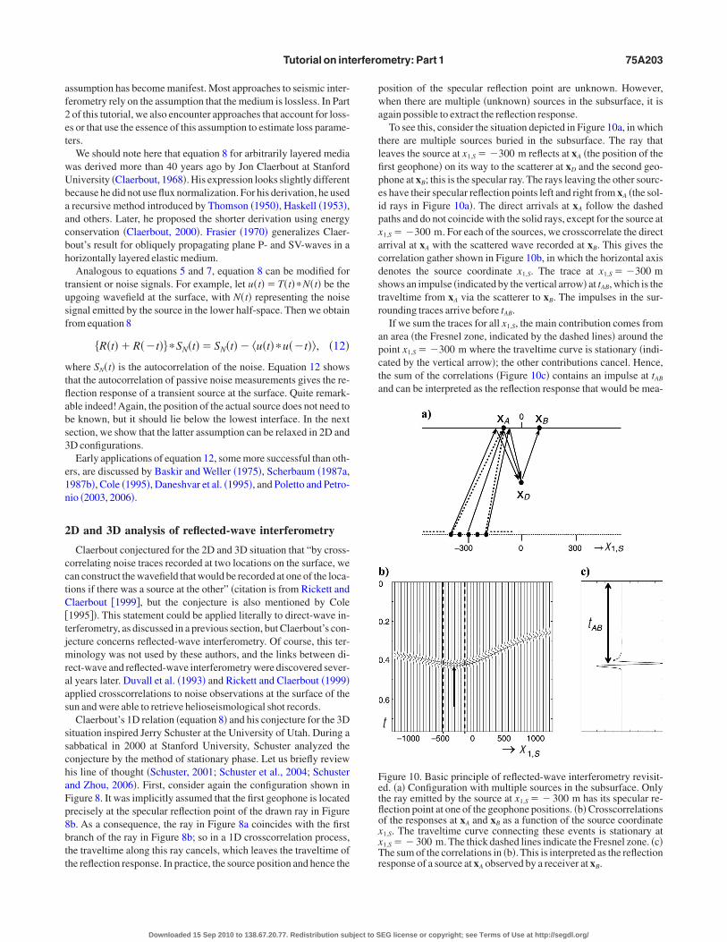
gain possible to extract the reflection response.To see this, consider the situation depicted in Figure 10a, in which

here are multiple sources buried in the subsurface. The ray thateaves the source at x1,S��300 m reflects at xA �the position of therst geophone� on its way to the scatterer at xD and the second geo-hone at xB; this is the specular ray. The rays leaving the other sourc-s have their specular reflection points left and right from xA �the sol-d rays in Figure 10a�. The direct arrivals at xA follow the dashedaths and do not coincide with the solid rays, except for the source at1,S��300 m. For each of the sources, we crosscorrelate the directrrival at xA with the scattered wave recorded at xB. This gives theorrelation gather shown in Figure 10b, in which the horizontal axisenotes the source coordinate x1,S. The trace at x1,S��300 mhows an impulse �indicated by the vertical arrow� at tAB, which is theraveltime from xA via the scatterer to xB. The impulses in the sur-ounding traces arrive before tAB.

If we sum the traces for all x1,S, the main contribution comes fromn area �the Fresnel zone, indicated by the dashed lines� around theoint x1,S��300 m where the traveltime curve is stationary �indi-ated by the vertical arrow�; the other contributions cancel. Hence,he sum of the correlations �Figure 10c� contains an impulse at tAB

nd can be interpreted as the reflection response that would be mea-

x

t

t

x

igure 10. Basic principle of reflected-wave interferometry revisit-d. �a� Configuration with multiple sources in the subsurface. Onlyhe ray emitted by the source at x1,S��300 m has its specular re-ection point at one of the geophone positions. �b� Crosscorrelationsf the responses at xA and xB as a function of the source coordinate1,S. The traveltime curve connecting these events is stationary at1,S��300 m. The thick dashed lines indicate the Fresnel zone. �c�he sum of the correlations in �b�. This is interpreted as the reflection

esponse of a source at x observed by a receiver at x .
A B

sbsxlpgl

soalmodx

tpdocsi

Ldat�afwtabopod2

t1fltscir

Fw


ured at xB if there were a source at xA. In other words, the source haseen repositioned from its unknown position at depth to a known po-ition xA at the surface. Note that this procedure works for any xA andB as long as the array of sources contains a source that emits a specu-ar ray via xA and the scatterer to xB. InAppendix A, we give a simpleroof that the stationary point of the traveltime curve in a correlationather corresponds to the source from which the rays to xA and xB

eave in the same direction.This example shows that it is possible to reposition �or redatum�

ources without knowing the velocity model and the position of theriginal sources. In exploration geophysics, redatuming is known asprocess that brings sources and/or receivers from the acquisition

evel to another depth level, using extrapolation operators based on aacro velocity model �Berryhill, 1979, 1984�. In seismic interfer-

metry, as illustrated in Figure 10, the extrapolation operator comesirectly from the data �in this example, the observed direct wave atA�.In the years following his sabbatical, Schuster showed that the in-

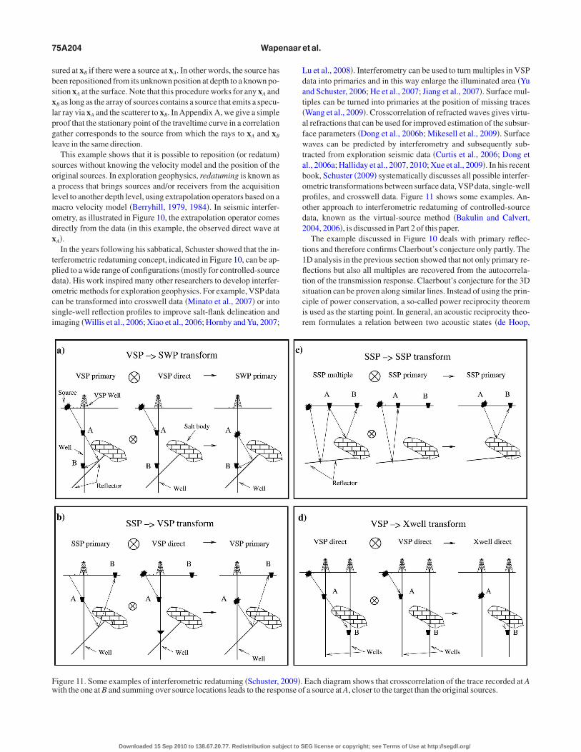
erferometric redatuming concept, indicated in Figure 10, can be ap-lied to a wide range of configurations �mostly for controlled-sourceata�. His work inspired many other researchers to develop interfer-metric methods for exploration geophysics. For example, VSP dataan be transformed into crosswell data �Minato et al., 2007� or intoingle-well reflection profiles to improve salt-flank delineation andmaging �Willis et al., 2006; Xiao et al., 2006; Hornby and Yu, 2007;

igure 11. Some examples of interferometric redatuming �Schuster,
ith the one at B and summing over source locations leads to the response o

u et al., 2008�. Interferometry can be used to turn multiples in VSPata into primaries and in this way enlarge the illuminated area �Yund Schuster, 2006; He et al., 2007; Jiang et al., 2007�. Surface mul-iples can be turned into primaries at the position of missing tracesWang et al., 2009�. Crosscorrelation of refracted waves gives virtu-l refractions that can be used for improved estimation of the subsur-ace parameters �Dong et al., 2006b; Mikesell et al., 2009�. Surfaceaves can be predicted by interferometry and subsequently sub-

racted from exploration seismic data �Curtis et al., 2006; Dong etl., 2006a; Halliday et al., 2007, 2010; Xue et al., 2009�. In his recentook, Schuster �2009� systematically discusses all possible interfer-metric transformations between surface data, VSPdata, single-wellrofiles, and crosswell data. Figure 11 shows some examples. An-ther approach to interferometric redatuming of controlled-sourceata, known as the virtual-source method �Bakulin and Calvert,004, 2006�, is discussed in Part 2 of this paper.

The example discussed in Figure 10 deals with primary reflec-ions and therefore confirms Claerbout’s conjecture only partly. TheD analysis in the previous section showed that not only primary re-ections but also all multiples are recovered from the autocorrela-

ion of the transmission response. Claerbout’s conjecture for the 3Dituation can be proven along similar lines. Instead of using the prin-iple of power conservation, a so-called power reciprocity theorems used as the starting point. In general, an acoustic reciprocity theo-em formulates a relation between two acoustic states �de Hoop,

Each diagram shows that crosscorrelation of the trace recorded at A
2009�. f a source at A, closer to the target than the original sources.

1trwcstie

nhat

HratmrmsoeTAaas

s�ure

nsf1arrttDd

rsTa

sn2dstStKt

pSn2cttsxw

FtnAicsaaAra


988; Fokkema and van den Berg, 1993�. One can distinguish be-ween convolution and correlation reciprocity theorems. The theo-ems of the correlation type reduce to power-conservation lawshen the two states are chosen identical, which is why they are also

alled power reciprocity theorems. Because reflection and transmis-ion responses are defined for downgoing and upgoing waves, forhe proof of Claerbout’s conjecture we make use of a correlation rec-procity theorem for �flux-normalized� one-way wavefields �Wap-naar and Grimbergen, 1996�.

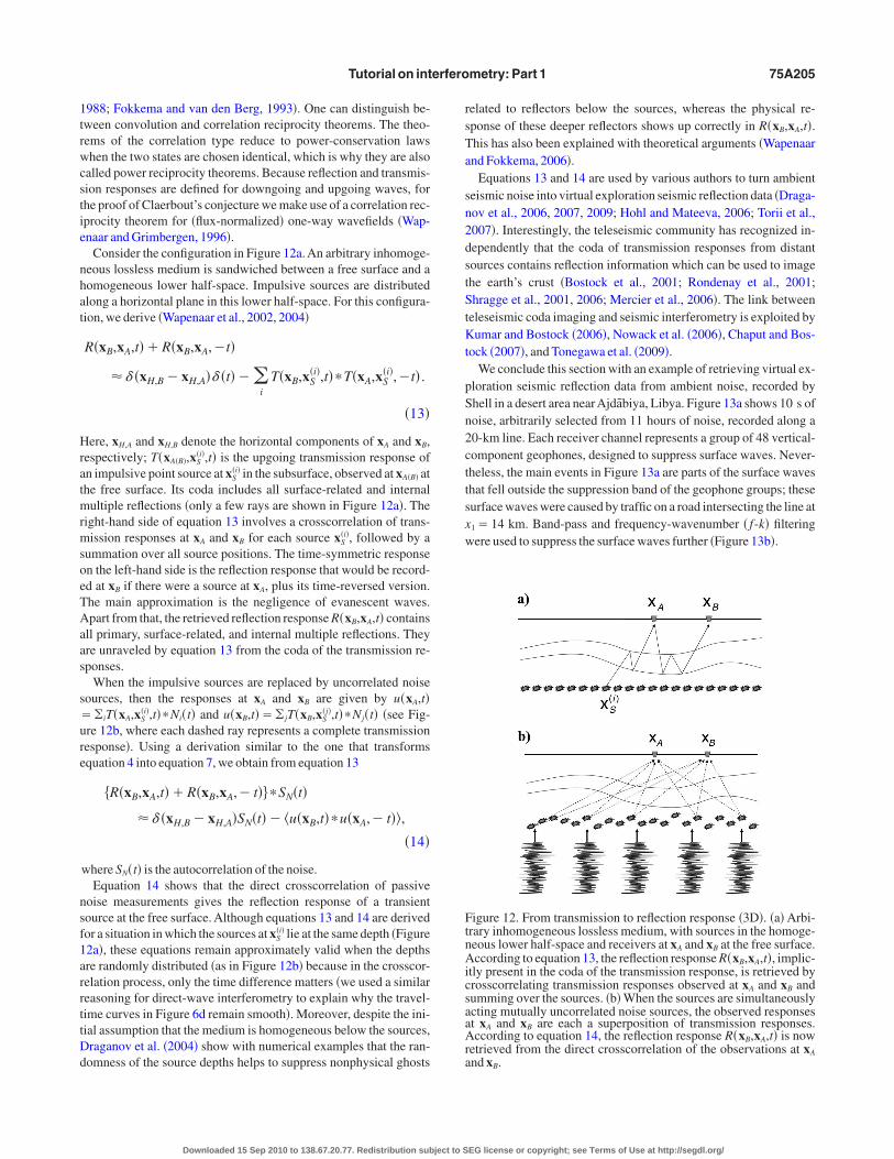
Consider the configuration in Figure 12a. An arbitrary inhomoge-eous lossless medium is sandwiched between a free surface and aomogeneous lower half-space. Impulsive sources are distributedlong a horizontal plane in this lower half-space. For this configura-ion, we derive �Wapenaar et al., 2002, 2004�

R�xB,xA,t��R�xB,xA,�t�

�� xH,B�xH,A�� t��i

T�xB,xS�i�,t��T�xA,xS

�i�,�t� .

�13�

ere, xH,A and xH,B denote the horizontal components of xA and xB,espectively; T�xA�B�,xS

�i�,t� is the upgoing transmission response ofn impulsive point source at xS

�i� in the subsurface, observed at xA�B� athe free surface. Its coda includes all surface-related and internal

ultiple reflections �only a few rays are shown in Figure 12a�. Theight-hand side of equation 13 involves a crosscorrelation of trans-ission responses at xA and xB for each source xS

�i�, followed by aummation over all source positions. The time-symmetric responsen the left-hand side is the reflection response that would be record-d at xB if there were a source at xA, plus its time-reversed version.he main approximation is the negligence of evanescent waves.part from that, the retrieved reflection response R�xB,xA,t� contains

ll primary, surface-related, and internal multiple reflections. Theyre unraveled by equation 13 from the coda of the transmission re-ponses.

When the impulsive sources are replaced by uncorrelated noiseources, then the responses at xA and xB are given by u�xA,t�

�iT�xA,xS�i�,t��Ni�t� and u�xB,t�� jT�xB,xS

�j�,t��Nj�t� �see Fig-re 12b, where each dashed ray represents a complete transmissionesponse�. Using a derivation similar to the one that transformsquation 4 into equation 7, we obtain from equation 13

�R�xB,xA,t��R�xB,xA,� t��SN�t�

�� xH,B�xH,A�SN�t�� u�xB,t��u�xA,� t�,

�14�

where SN�t� is the autocorrelation of the noise.Equation 14 shows that the direct crosscorrelation of passive

oise measurements gives the reflection response of a transientource at the free surface. Although equations 13 and 14 are derivedor a situation in which the sources at xS

�i� lie at the same depth �Figure2a�, these equations remain approximately valid when the depthsre randomly distributed �as in Figure 12b� because in the crosscor-elation process, only the time difference matters �we used a similareasoning for direct-wave interferometry to explain why the travel-ime curves in Figure 6d remain smooth�. Moreover, despite the ini-ial assumption that the medium is homogeneous below the sources,raganov et al. �2004� show with numerical examples that the ran-omness of the source depths helps to suppress nonphysical ghosts


elated to reflectors below the sources, whereas the physical re-ponse of these deeper reflectors shows up correctly in R�xB,xA,t�.his has also been explained with theoretical arguments �Wapenaarnd Fokkema, 2006�.

Equations 13 and 14 are used by various authors to turn ambienteismic noise into virtual exploration seismic reflection data �Draga-ov et al., 2006, 2007, 2009; Hohl and Mateeva, 2006; Torii et al.,007�. Interestingly, the teleseismic community has recognized in-ependently that the coda of transmission responses from distantources contains reflection information which can be used to imagehe earth’s crust �Bostock et al., 2001; Rondenay et al., 2001;hragge et al., 2001, 2006; Mercier et al., 2006�. The link between

eleseismic coda imaging and seismic interferometry is exploited byumar and Bostock �2006�, Nowack et al. �2006�, Chaput and Bos-

ock �2007�, and Tonegawa et al. �2009�.We conclude this section with an example of retrieving virtual ex-

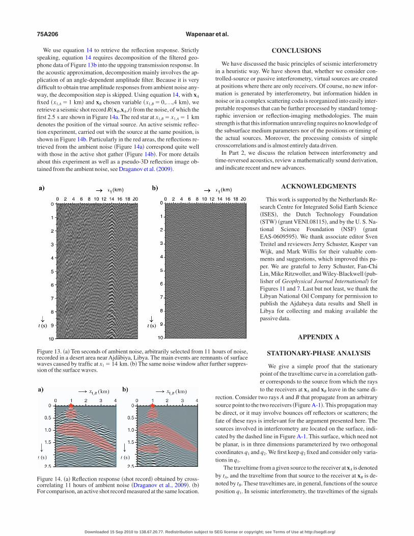
loration seismic reflection data from ambient noise, recorded byhell in a desert area nearAjdābiya, Libya. Figure 13a shows 10 s ofoise, arbitrarily selected from 11 hours of noise, recorded along a0-km line. Each receiver channel represents a group of 48 vertical-omponent geophones, designed to suppress surface waves. Never-heless, the main events in Figure 13a are parts of the surface waveshat fell outside the suppression band of the geophone groups; theseurface waves were caused by traffic on a road intersecting the line at

1�14 km. Band-pass and frequency-wavenumber � f-k� filteringere used to suppress the surface waves further �Figure 13b�.

igure 12. From transmission to reflection response �3D�. �a� Arbi-rary inhomogeneous lossless medium, with sources in the homoge-eous lower half-space and receivers at xA and xB at the free surface.ccording to equation 13, the reflection response R�xB,xA,t�, implic-

tly present in the coda of the transmission response, is retrieved byrosscorrelating transmission responses observed at xA and xB andumming over the sources. �b� When the sources are simultaneouslycting mutually uncorrelated noise sources, the observed responsest xA and xB are each a superposition of transmission responses.ccording to equation 14, the reflection response R�xB,xA,t� is now

etrieved from the direct crosscorrelation of the observations at xA

nd x .
B

sptpdwfirfidtstwat

itamnprsttc

ta

rsbfscbct

bnp

Frws

FcF


We use equation 14 to retrieve the reflection response. Strictlypeaking, equation 14 requires decomposition of the filtered geo-hone data of Figure 13b into the upgoing transmission response. Inhe acoustic approximation, decomposition mainly involves the ap-lication of an angle-dependent amplitude filter. Because it is veryifficult to obtain true amplitude responses from ambient noise any-ay, the decomposition step is skipped. Using equation 14, with xA

xed �x1,A�1 km� and xB chosen variable �x1,B�0,. . .,4 km�, weetrieve a seismic shot record R�xB,xA,t� from the noise, of which therst 2.5 s are shown in Figure 14a. The red star at x1,B�x1,A�1 kmenotes the position of the virtual source. An active seismic reflec-ion experiment, carried out with the source at the same position, ishown in Figure 14b. Particularly in the red areas, the reflections re-rieved from the ambient noise �Figure 14a� correspond quite wellith those in the active shot gather �Figure 14b�. For more details

bout this experiment as well as a pseudo-3D reflection image ob-ained from the ambient noise, see Draganov et al. �2009�.

1(km)

igure 13. �a� Ten seconds of ambient noise, arbitrarily selected fromecorded in a desert area near Ajdābiya, Libya. The main events areaves caused by traffic at x1�14 km. �b� The same noise window a

ion of the surface waves.

igure 14. �a� Reflection response �shot record� obtained by cross-orrelating 11 hours of ambient noise �Draganov et al., 2009�. �b�or comparison, an active shot record measured at the same location.


CONCLUSIONS

We have discussed the basic principles of seismic interferometryn a heuristic way. We have shown that, whether we consider con-rolled-source or passive interferometry, virtual sources are createdt positions where there are only receivers. Of course, no new infor-ation is generated by interferometry, but information hidden in

oise or in a complex scattering coda is reorganized into easily inter-retable responses that can be further processed by standard tomog-aphic inversion or reflection-imaging methodologies. The maintrength is that this information unraveling requires no knowledge ofhe subsurface medium parameters nor of the positions or timing ofhe actual sources. Moreover, the processing consists of simplerosscorrelations and is almost entirely data driven.

In Part 2, we discuss the relation between interferometry andime-reversed acoustics, review a mathematically sound derivation,nd indicate recent and new advances.

ACKNOWLEDGMENTS

This work is supported by the Netherlands Re-search Centre for Integrated Solid Earth Science�ISES�, the Dutch Technology Foundation�STW� �grant VENI.08115�, and by the U. S. Na-tional Science Foundation �NSF� �grantEAS-0609595�. We thank associate editor SvenTreitel and reviewers Jerry Schuster, Kasper vanWijk, and Mark Willis for their valuable com-ments and suggestions, which improved this pa-per. We are grateful to Jerry Schuster, Fan-ChiLin, Mike Ritzwoller, and Wiley-Blackwell �pub-lisher of Geophysical Journal International� forFigures 11 and 7. Last but not least, we thank theLibyan National Oil Company for permission topublish the Ajdabeya data results and Shell inLibya for collecting and making available thepassive data.

APPENDIX A

STATIONARY-PHASE ANALYSIS

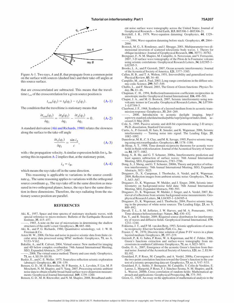
We give a simple proof that the stationarypoint of the traveltime curve in a correlation gath-er corresponds to the source from which the raysto the receivers at xA and xB leave in the same di-

ection. Consider two rays A and B that propagate from an arbitraryource point to the two receivers �Figure A-1�. This propagation maye direct, or it may involve bounces off reflectors or scatterers; theate of these rays is irrelevant for the argument presented here. Theources involved in interferometry are located on the surface, indi-ated by the dashed line in Figure A-1. This surface, which need note planar, is in three dimensions parameterized by two orthogonaloordinates q1 and q2. We first keep q2 fixed and consider only varia-ions in q1.

The traveltime from a given source to the receiver at xA is denotedy tA, and the traveltime from that source to the receiver at xB is de-oted by tB. These traveltimes are, in general, functions of the sourceosition q . In seismic interferometry, the traveltimes of the signals

1(km)

urs of noise,nts of surfacether suppres-

11 horemnafter fur

1


tt

T

Aa

ws

w

nsstt

A

—

A

A

B

—

B

B

B

B

—

B

B

B

C

C

C

C

C

C

—

C

C

D

d

D

D

D

D

D

D

D

F

F

F

G

G

G

G

G

Fot


hat are crosscorrelated are subtracted. This means that the travel-ime tcorr of the crosscorrelation for a given source position is

tcorr�q1�� tB�q1�� tA�q1� . �A-1�

he condition that the traveltime is stationary means that

�tcorr�q1��q1

��tB�q1�

�q1�

�tA�q1��q1

�0. �A-2�

standard derivation �Aki and Richards, 1980� relates the slownesslong the surface to the take-off angle

�tA�q1��q1

�sin iA

c, �A-3�

ith c the propagation velocity.Asimilar expression holds for tB. In-erting this in equation A-2 implies that, at the stationary point,

iA� iB, �A-4�

hich means the rays take off in the same direction.This reasoning is applicable to variations in the source coordi-

ate q1. The same reasoning applies to variations with the orthogonalource coordinate q2. The rays take off in the same direction as mea-ured in two orthogonal planes; hence, the rays have the same direc-ion in three dimensions. Therefore, the rays radiating from the sta-ionary source position are parallel.

REFERENCES

ki, K., 1957, Space and time spectra of stationary stochastic waves, withspecial reference to micro-tremors: Bulletin of the Earthquake ResearchInstitute, 35, 415–457.—–, 1965, A note on the use of microseisms in determining the shallowstructures of the earth’s crust: Geophysics, 30, 665–666.

ki, K., and P. G. Richards, 1980, Quantitative seismology, vol. 1: W. H.Freeman & Co.

sten M. W., 2006, On bias and noise in passive seismic data from finite cir-cular array data processed using SPAC methods: Geophysics, 71, no. 6,V153–V162.

akulin, A., and R. Calvert, 2004, Virtual source: New method for imagingand 4D below complex overburden: 74th Annual International Meeting,SEG, ExpandedAbstracts, 2477–2480.—–, 2006, The virtual source method: Theory and case study: Geophysics,71, no. 4, SI139–SI150.

askir, E., and C. E. Weller, 1975, Sourceless reflection seismic exploration�abstract�: Geophysics, 40, 158–159.

ensen, G. D., M. H. Ritzwoller, M. P. Barmin, A. L. Levshin, F. Lin, M. P.Moschetti, N. M. Shapiro, and Y. Yang, 2007, Processing seismic ambientnoise data to obtain reliable broad-band surface wave dispersion measure-ments: Geophysical Journal International, 169, 1239–1260.

ensen, G. D., M. H. Ritzwoller, and N. M. Shapiro, 2008, Broadband ambi-

igure A-1. Two rays, A and B, that propagate from a common pointn the surface with sources �dashed line� and their take-off angles athis source surface.


ent noise surface wave tomography across the United States: Journal ofGeophysical Research — Solid Earth, 113, B05306-1–B05306-21.

erryhill, J. R., 1979, Wave-equation datuming: Geophysics, 44, 1329–1344.—–, 1984, Wave-equation datuming before stack: Geophysics, 49, 2064–2066.

ostock, M. G., S. Rondenay, and J. Shragge, 2001, Multiparameter two-di-mensional inversion of scattered teleseismic body waves. 1. Theory foroblique incidence: Journal of Geophysical Research, 106, 30771–30782.

renguier, F., N. M. Shapiro, M. Campillo, A. Nercessian, and V. Ferrazzini,2007, 3-D surface wave tomography of the Piton de la Fournaise volcanousing seismic correlations: Geophysical Research Letters, 34, L02305-1–L02305-5.

rooks, L. A., and P. Gerstoft, 2007, Ocean acoustic interferometry: Journalof theAcoustical Society ofAmerica, 121, 3377–3385.

allen, H. B., and T. A. Welton, 1951, Irreversibility and generalized noise:Physical Review, 83, 34–40.

ampillo, M., and A. Paul, 2003, Long-range correlations in the diffuse seis-mic coda: Science, 299, 547–549.

hallis, L., and F. Sheard, 2003, The Green of Green functions: Physics To-day, 56, 41–46.

hapman, C. H., 1994, Reflection/transmission coefficients reciprocities inanisotropic media: Geophysical Journal International, 116, 498–501.

haput, J. A., and M. G. Bostock, 2007, Seismic interferometry using non-volcanic tremor in Cascadia: Geophysical Research Letters, 34, L07304-1–L07304-5.

laerbout, J. F., 1968, Synthesis of a layered medium from its acoustic trans-mission response: Geophysics, 33, 264–269.—–, 2000, Introduction to acoustic daylight imaging, http://sepwww.stanford.edu/data/media/public/sep//jon/eqcor/index.html, ac-cessed 21 May 2010.

ole, S., 1995, Passive seismic and drill-bit experiments using 2-D arrays:Ph.D. dissertation, Stanford University.

urtis, A., P. Gerstoft, H. Sato, R. Snieder, and K. Wapenaar, 2006, Seismicinterferometry — Turning noise into signal: The Leading Edge, 25,1082–1092.

aneshvar, M. R., C. S. Clay, and M. K. Savage, 1995, Passive seismic imag-ing using microearthquakes: Geophysics, 60, 1178–1186.

e Hoop, A. T., 1988, Time-domain reciprocity theorems for acoustic wavefields in fluids with relaxation: Journal of theAcoustical Society ofAmeri-ca, 84, 1877–1882.

ong, S., R. He, and G. T. Schuster, 2006a, Interferometric prediction andleast squares subtraction of surface waves: 76th Annual InternationalMeeting, SEG, ExpandedAbstracts, 2783–2786.

ong, S., J. Sheng, and G. T. Schuster, 2006b, Theory and practice of refrac-tion interferometry: 76th Annual International Meeting, SEG, ExpandedAbstracts, 3021–3025.

raganov, D., X. Campman, J. Thorbecke, A. Verdel, and K. Wapenaar,2009, Reflection images from ambient seismic noise: Geophysics, 74, no.5, A63–A67.

raganov, D., K. Wapenaar, W. Mulder, and J. Singer, 2006, Seismic inter-ferometry on background-noise field data: 76th Annual InternationalMeeting, SEG, ExpandedAbstracts, 590–593.

raganov, D., K. Wapenaar, W. Mulder, J. Singer, and A. Verdel, 2007, Re-trieval of reflections from seismic background-noise measurements: Geo-physical Research Letters, 34, L04305-1–L04305-4.

raganov, D., K. Wapenaar, and J. Thorbecke, 2004, Passive seismic imag-ing in the presence of white noise sources: The Leading Edge, 23, no. 9,889–892.

uvall, T. L., S. M. Jefferies, J. W. Harvey, and M. A. Pomerantz, 1993,Time-distance helioseismology: Nature, 362, 430–432.

an, Y., and R. Snieder, 2009, Required source distribution for interferome-try of waves and diffusive fields: Geophysical Journal International, 179,1232–1244.

okkema, J. T., and P. M. van den Berg, 1993, Seismic applications of acous-tic reciprocity: Elsevier Scientific Publ. Co., Inc.

rasier, C. W., 1970, Discrete time solution of plane P-SV waves in a planelayered medium: Geophysics, 35, 197–219.

erstoft, P., K. G. Sabra, P. Roux, W. A. Kuperman, and M. C. Fehler, 2006,Green’s functions extraction and surface-wave tomography from mi-croseisms in southern California: Geophysics, 71, no. 4, SI23–SI31.

odin, O. A., 2007, Emergence of the acoustic Green’s function from ther-mal noise: Journal of theAcoustical Society ofAmerica, 121, no. 2, EL96–EL102.

ouédard, P., P. Roux, M. Campillo, and A. Verdel, 2008a, Convergence ofthe two-point correlation function toward the Green’s function in the con-text of a seismic-prospecting data set: Geophysics, 73, no. 6, V47–V53.

ouédard, P., L. Stehly, F. Brenguier, M. Campillo, Y. Colin de Verdière, E.Larose, L. Margerin, P. Roux, F. J. Sánchez-Sesma, N. M. Shapiro, and R.L. Weaver, 2008b, Cross-correlation of random fields: Mathematical ap-proach and applications: Geophysical Prospecting, 56, 375–393.

reen, G., 1828, An essay on the application of mathematical analysis to the


H

H

H

H

H

H

H

J

K

K

K

L

L

L

L

L

L

L

L

L

L

M

M

M

M

M

M

N

O—

P

P

P

—

R

R

R

R

R

R

S

—

S

S

S

—

S

—S

S

S

S

S

S

S

S


theories of electricity and magnetism: Privately published.alliday, D. F., A. Curtis, J. O.A. Robertsson, and D.-J. van Manen, 2007, In-terferometric surface-wave isolation and removal: Geophysics, 72, no. 5,A69–A73.

alliday, D. F., A. Curtis, P. Vermeer, C. Strobbia, A. Glushchenko, D.-J. vanManen, and J. O.A. Robertsson, 2010, Interferometric ground-roll remov-al: Attenuation of scattered surface waves in single-sensor data: Geophys-ics, 75, no. 2, SA15–SA25

askell, N. A., 1953, The dispersion of surface waves on multilayered me-dia: Bulletin of the Seismological Society ofAmerica, 43, 17–34.

e, R., B. Hornby, and G. Schuster, 2007, 3D wave-equation interferometricmigration of VSP free-surface multiples: Geophysics, 72, no. 5, S195–S203.

enstridge, J. D., 1979, A signal processing method for circular arrays: Geo-physics, 44, 179–184.

ohl, D., and A. Mateeva, 2006, Passive seismic reflectivity imaging withocean-bottom cable data: 76th Annual International Meeting, SEG, Ex-pandedAbstracts, 1560–1563.

ornby, B. E., and J. Yu, 2007, Interferometric imaging of a salt flank usingwalkaway VSP data: The Leading Edge, 26, 760–763.

iang, Z., J. Sheng, J. Yu, G. T. Schuster, and B. E. Hornby, 2007, Migrationmethods for imaging different-order multiples: Geophysical Prospecting55, 1–19.

ang, T.-S., and J. S. Shin, 2006, Surface-wave tomography from ambientseismic noise of accelerograph networks in southern Korea: GeophysicalResearch Letters, 33, L17303-1–L17303-5.

ennett, B. L. N., N. J. Kerry, and J. H. Woodhouse, 1978, Symmetries in thereflection and transmission of elastic waves: Geophysical Journal of theRoyalAstronomical Society, 52, 215–230.

umar, M. R., and M. G. Bostock, 2006, Transmission to reflection transfor-mation of teleseismic wavefields: Journal of Geophysical Research —Solid Earth, 111, B08306-1–B08306-9.

arose, E., A. Khan, Y. Nakamura, and M. Campillo, 2005, Lunar subsurfaceinvestigated from correlation of seismic noise: Geophysical Research Let-ters, 32, L16201-1–L16201-4.

arose, E., L. Margerin, A. Derode, B. van Tiggelen, M. Campillo, N. Sha-piro, A. Paul, L. Stehly, and M. Tanter, 2006, Correlation of random wavefields:An interdisciplinary review: Geophysics, 71, no. 4, SI11–SI21.

e Bellac, M., F. Mortessagne, and G. G. Batrouni, 2004, Equilibrium andnon-equilibrium statistical thermodynamics: Cambridge University Press.

i, H., W. Su, C.-Y. Wang, and Z. Huang, 2009, Ambient noise Rayleighwave tomography in western Sichuan and eastern Tibet: Earth and Plane-tary Science Letters, 282, 201–211.

iang, C., and C. A. Langston, 2008, Ambient seismic noise tomography andstructure of eastern North America: Journal of Geophysical Research —Solid Earth, 113, B03309-1–B03309-18.

in, F.-C., M. P. Moschetti, and M. H. Ritzwoller, 2008, Surface wave to-mography of the western United States from ambient seismic noise: Ray-leigh and Love wave phase velocity maps: Geophysical Journal Interna-tional, 173, 281–298.

in, F.-C., M. H. Ritzwoller, and R. Snieder, 2009, Eikonal tomography: Sur-face wave tomography by phase front tracking across a regional broad-band seismic array: Geophysical Journal International, 177, 1091–1110.

obkis, O. I., and R. L. Weaver, 2001, On the emergence of the Green’s func-tion in the correlations of a diffuse field: Journal of the Acoustical SocietyofAmerica, 110, 3011–3017.

onguet-Higgins, M. S., 1950, A theory for the generation of microseisms:Philosophical Transactions of the Royal Society of London Series A, 243,1–35.

u, R., M. Willis, X. Campman, J. Ajo-Franklin, and M. N. Toksöz, 2008,Redatuming through a salt canopy and target-oriented salt-flank imaging:Geophysics 73, no. 3, S63–S71.a, S., G. A. Prieto, and G. C. Beroza, 2008, Testing community velocitymodels for southern California using the ambient seismic field: Bulletin ofthe Seismological Society ofAmerica, 98, 2694–2714.alcolm, A. E., J. A. Scales, and B. A. van Tiggelen, 2004, Extracting theGreen function from diffuse, equipartitioned waves: Physical Review E,70, 015601�R�-1–015601�R�-4.ercier, J.-P., M. G. Bostock, and A. M. Baig, 2006, Improved Green’s func-tions for passive-source structural studies: Geophysics, 71, no. 4, SI95–SI102.ikesell, D., K. van Wijk, A. Calvert, and M. Haney, 2009, The virtual re-fraction: Useful spurious energy in seismic interferometry: Geophysics,74, no. 3, A13–A17.inato, S., K. Onishi, T. Matsuoka, Y. Okajima, J. Tsuchiyama, D. Nobuoka,H. Azuma, and T. Iwamoto, 2007, Cross-well seismic survey withoutborehole source: 77th Annual International Meeting, SEG, Expanded Ab-stracts, 1357–1361.iyazawa, M., R. Snieder, and A. Venkataraman, 2008, Application of seis-mic interferometry to extract P- and S-wave propagation and observationof shear-wave splitting from noise data at Cold Lake, Alberta, Canada:Geophysics, 73, no. 4, D35–D40.


owack, R. L., S. Dasgupta, G. T. Schuster, and J.-M. Sheng, 2006, Correla-tion migration using Gaussian beams of scattered teleseismic body waves:Bulletin of the Seismological Society ofAmerica, 96, 1–10.

kada, H., 2003, The microtremor survey method: SEG.—–, 2006, Theory of efficient array observations of microtremors withspecial reference to the SPAC method: Exploration Geophysics, 37,73–85.

erton, M., F. J. Sánchez-Sesma, A. Rodríguez-Castellanos, M. Campillo,and R. L. Weaver, 2009, Two perspectives on equipartition in diffuse elas-tic fields in three dimensions: Journal of the Acoustical Society of Ameri-ca, 126, 1125–1130.

icozzi, M., S. Parolai, D. Bindi, and A. Strollo, 2009, Characterization ofshallow geology by high-frequency seismic noise tomography: Geophysi-cal Journal International, 176, 164–174.

oletto, F., and L. Petronio, 2003, Transmitted and reflected waves in tunnelSWD: 73rd Annual International Meeting, SEG, Expanded Abstracts,1211–1214.—–, 2006, Seismic interferometry with a TBM source of transmitted andreflected waves: Geophysics, 71, no. 4, SI85–SI93.

amírez, A. C., and A. B. Weglein, 2009, Green’s theorem as a comprehen-sive framework for data reconstruction, regularization, wavefield separa-tion, seismic interferometry, and wavelet estimation: A tutorial: Geophys-ics, 74, no. 6, W35–W62.

ickett, J., and J. Claerbout, 1999, Acoustic daylight imaging via spectralfactorization: Helioseismology and reservoir monitoring: The LeadingEdge, 18, 957–960.

ondenay, S., M. G. Bostock, and J. Shragge, 2001, Multiparameter two-di-mensional inversion of scattered teleseismic body waves. 3.Application tothe Cascadia 1993 data set: Journal of Geophysical Research, 106, 30795–30807.

oux, P., and M. Fink, 2003, Green’s function estimation using secondarysources in a shallow water environment: Journal of the Acoustical SocietyofAmerica, 113, 1406–1416.

ytov, S. M., 1956, On thermal fluctuations in distributed systems: DokladyAkademii Nauk SSSR, 110, 371.

ytov, S. M., Y. A. Kravtsov, and V. I. Tatarskii, 1989, Principles of statisticalradiophysics. 3: Elements of random fields: Springer-Verlag Berlin.

abra, K. G., P. Gerstoft, P. Roux, W. A. Kuperman, and M. C. Fehler, 2005a,Extracting time-domain Green’s function estimates from ambient seismicnoise: Geophysical Research Letters, 32, L03310-1–L03310-5.—–, 2005b, Surface wave tomography from microseisms in southern Cali-fornia: Geophysical Research Letters, 32, L14311-1–L14311-4.

abra, K. G., P. Roux, and W. A. Kuperman, 2005c, Arrival-time structure ofthe time-averaged ambient noise cross-correlation function in an oceanicwaveguide: Journal of theAcoustical Society ofAmerica, 117, no. 1, 164–174.

ánchez-Sesma, F. J., J. A. Pérez-Ruiz, M. Campillo, and F. Luzón, 2006,Elastodynamic 2D Green function retrieval from cross-correlation: Ca-nonical inclusion problem: Geophysical Research Letters, 33, L13305-1–L13305-6.

cherbaum, F., 1987a, Seismic imaging of the site response using micro-earthquake recordings. Part I. Method: Bulletin of the Seismological Soci-ety ofAmerica, 77, 1905–1923.—–, 1987b, Seismic imaging of the site response using microearthquakerecordings. Part II. Application to the Swabian Jura, southwest Germany,seismic network: Bulletin of the Seismological Society of America, 77,1924–1944.

chuster, G. T., 2001, Theory of daylight/interferometric imaging: Tutorial:63rd Conference & Technical Exhibition, EAGE, Extended Abstracts,A32.—–, 2009, Seismic interferometry: Cambridge University Press.

chuster, G. T., J. Yu, J. Sheng, and J. Rickett, 2004, Interferometric/daylightseismic imaging: Geophysical Journal International, 157, 838–852.

chuster, G. T., and M. Zhou, 2006, A theoretical overview of model-basedand correlation-based redatuming methods: Geophysics, 71, no. 4, SI103–SI110.

hapiro, N. M., and M. Campillo, 2004, Emergence of broadband Rayleighwaves from correlations of the ambient seismic noise: Geophysical Re-search Letters, 31, L07614-1–L07614-4.

hapiro, N. M., M. Campillo, L. Stehly, and M. H. Ritzwoller, 2005, High-resolution surface-wave tomography from ambient seismic noise: Sci-ence, 307, 1615–1618.

hragge, J., B. Artman, and C. Wilson, 2006, Teleseismic shot-profile migra-tion: Geophysics, 71, no. 4, SI221–SI229.

hragge, J., M. G. Bostock, and S. Rondenay, 2001, Multiparameter two-di-mensional inversion of scattered teleseismic body waves. 2. Numericalexamples: Journal of Geophysical Research, 106, 30783–30793.

nieder, R., 2004, Extracting the Green’s function from the correlation ofcoda waves: A derivation based on stationary phase: Physical Review E,69, 046610-1–046610-8.

nieder, R., K. Wapenaar, and U. Wegler, 2007, Unified Green’s function re-trieval by cross-correlation: Connection with energy principles: Physical


S

T

T

T

T

T

U

v

W

W

W

W

W

W

W

—

W

W

X

X

Y

Y

Y

Y

Y


Review E, 75, 036103-1–036103-14.tehly, L., M. Campillo, and N. M. Shapiro, 2006, A study of the seismicnoise from its long-range correlation properties: Journal of GeophysicalResearch, 111, B10306-1–B10306-12.

hompson, A. R., J. M. Moran, and G. W. Swenson Jr., 2001, Interferometryand synthesis in radio astronomy: Wiley Interscience.

homson, W. T., 1950, Transmission of elastic waves through a stratified sol-id medium: Journal ofApplied Physics, 21, 89–93.

oksöz, M. N., 1964, Microseisms and an attempted application to explora-tion: Geophysics, 39, 154–177.

onegawa, T., K. Nishida, T. Watanabe, and K. Shiomi, 2009, Seismic inter-ferometry of teleseismic S-wave coda for retrieval of body waves: An ap-plication to the Philippine Sea slab underneath the Japanese Islands: Geo-physical Journal International, 178, 1574–1586.

orii, K., T. Matsuoka, K. Onishi, K. Shirashi, T. Aizawa, Y. Yamanaka, S.Ito, T. Kimura, Y. Asano, and T. Takeda, 2007, Application of seismic in-terferometry to natural earthquakes measured by small-scale array: 77thAnnual International Meeting, SEG, ExpandedAbstracts, 1362–1366.

rsin, B., 1983, Review of elastic and electromagnetic wave propagation inhorizontally layered media: Geophysics, 48, 1063–1081.

an Tiggelen, B. A., 2003, Green function retrieval and time reversal in a dis-ordered world: Physical Review Letters, 91, 243904-1–243904-4.ang, Y., Y. Luo, and G. T. Schuster, 2009, Interferometric interpolation ofmissing seismic data: Geophysics, 74, no. 3, SI37–SI45.apenaar, K., D. Draganov, J. Thorbecke, and J. Fokkema, 2002, Theory ofacoustic daylight imaging revisited: 72nd Annual International Meeting,SEG, ExpandedAbstracts, 2269–2272.apenaar, K., and J. Fokkema, 2006, Green’s function representations forseismic interferometry: Geophysics, 71, no. 4, SI33–SI46.apenaar, C. P. A., and J. L. T. Grimbergen, 1996, Reciprocity theorems forone-way wave fields: Geophysical Journal International, 127, 169–177.apenaar, K., J. Thorbecke, and D. Draganov, 2004, Relations between re-flection and transmission responses of three-dimensional inhomogeneousmedia: Geophysical Journal International, 156, 179–194.eaver, R., B. Froment, and M. Campillo, 2009, On the correlation of non-isotropically distributed ballistic scalar diffuse waves: Journal of the


Acoustical Society ofAmerica, 126, 1817–1826.eaver, R. L., and O. I. Lobkis, 2001, Ultrasonics without a source: Thermalfluctuation correlations at MHz frequencies: Physical Review Letters, 87,134301-1–134301-4.—–, 2002, On the emergence of the Green’s function in the correlations ofa diffuse field: Pulse-echo using thermal phonons: Ultrasonics, 40,435–439.ebb, S. C., 1998, Broadband seismology and noise under the ocean: Re-views of Geophysics, 36, 105–142.illis, M. E., R. Lu, X. Campman, M. N. Toksöz, Y. Zhang, and M. V. deHoop, 2006, A novel application of time-reversed acoustics: Salt-domeflank imaging using walkaway VSP surveys: Geophysics, 71, no. 2, A7–A11.

iao, X., M. Zhou, and G. T. Schuster, 2006, Salt-flank delineation by inter-ferometric imaging of transmitted P- and S-waves: Geophysics, 71, no. 4,SI197–SI207.

ue, Y., S. Dong, and G. T. Schuster, 2009, Interferometric prediction andsubtraction of surface waves with a nonlinear local filter: Geophysics, 74,no. 1, SI1–SI8.

ao, H., X. Campman, M. V. de Hoop, and R. D. van der Hilst, 2009, Estima-tion of surface wave Green’s functions from correlation of direct waves,coda waves, and ambient noise in SE Tibet: Physics of the Earth and Plane-tary Interiors, 177, 1–11.

ao, H., R. D. van der Hilst, and M. V. de Hoop, 2006, Surface-wave array to-mography in SE Tibet from ambient seismic noise and two-station analysis— I. Phase velocity maps: Geophysical Journal International, 166,732–744.

ao, H., C. Beghein, and R. D. van der Hilst, 2008, Surface-wave array to-mography in SE Tibet from ambient seismic noise and two-station analysis— II. Crustal and upper-mantle structure: Geophysical Journal Interna-tional, 173, 205–219.

okoi, T., and S. Margaryan, 2008, Consistency of the spatial autocorrelationmethod with seismic interferometry and its consequence: GeophysicalProspecting, 56, 435–451.

u, J., and G. T. Schuster, 2006, Crosscorrelogram migration of inverse verti-cal seismic profile data: Geophysics, 71, no. 1, S1–S11.


tutorial on seismic interferometry: part 1 — basic...

Documents