Modelling Portfolio Capital Flows in a Global Framework:

Multilateral Implications of Capital Controls

Gianna Boeroa, Zeyyad Mandalincib, Mark P. Taylorc

aDepartment of Economics, University of Warwick, UKbSchool of Economics and Finance, Queen Mary University of London, UK

cWarwick Business School, University of Warwick, UK andCentre for Economic Policy Research

June 2, 2016

Abstract

In the aftermath of the global financial crisis, many emerging market countriesresorted to capital controls to tackle the excessive surge of capital inflows. A numberof recent research papers have suggested that the imposition of controls may haveimposed negative externalities on other countries by deflecting flows. Our aim inthe research reported in this paper is to construct a comprehensive global economet-ric model which captures the dynamic interactions of capital flows with domestic andglobal fundamentals, and to assess the efficacy of capital controls and potential deflec-tion effects on other countries. The results suggest that capital controls are effectivefor some countries in the short run, but have no lasting effects. Moreover, there is onlylimited evidence of deflection effects for a small number of emerging market countries.

Keywords: Portfolio Capital Flows, Global VAR (GVAR), Capital Controls, Emerg-ing Markets.

JEL Classification: C32, C5, F32, F42, G11.

Acknowledgements: The authors are grateful to Menzie Chinn, Kristin Forbes, AshokaMody, Jonathan Ostry and Frank Warnock for constructive comments on a previousversion, although any errors remaining are the responsibility of the authors.

1 Introduction

Since the mid-1980s, emerging markets have experienced a rapid increase in financialinvestment from the rest of the world. While there are many gains from global financialintegration (see e.g. Kose et al., 2009), the experience of the last few decades suggeststhat opening up domestic markets to free capital flows does introduce various risks forrecipient countries. Concerns have been raised, for example, during and in the wake ofthe recent global financial crisis, with many countries facing a sudden collapse followedby a surge in capital flows.1

1The possible impact of surges in capital flows on the macroeconomy may not only be confined todeveloping countries, moreover. For example, Laibson & Mollerstrom (2010) argue that the global financialcrisis itself may have been caused and certainly exacerbated by international financial flows chasing highasset returns in markets characterized by bubbles, in contrast to the global savings glut explanation ofthe global crisis advocated by Bernanke (2005) and others.

1

These events have brought about a renewed interest in the application of capitalcontrols and in their effectiveness as a policy tool to manage capital flows. As notedby Forbes et al. (2012), even erstwhile advocates of capital market liberalization suchas the International Monetary Fund (IMF) have in recent years become supportive ofthe judicious use of capital controls. This debate has been boosted by a series of policyand research papers, most notably from the IMF, providing guidance for countries andrecommendations on how to design appropriate policy responses to changes in capitalflows. In a recent IMF Staff Discussion Note, Ostry et al. (2012) recognize the useof capital controls as legitimate under certain conditions and argue that multilateralconsiderations must be taken into account in assessing the merits of capital controls atthe individual country level, including taking into account the possible externalities forother countries in the form of deflection of flows.

However, empirically documenting and studying these effects is complex, as one mustdisentangle various domestic and international dependencies that drive capital flows, andthis requires a comprehensive global perspective. It is well known that omitting relevantinformation in empirical models can easily lead to incorrect conclusions. Hence, ourambitious objective in the research reported in this paper is to construct an empiricalmodel of the global economy that is sufficiently sophisticated as to be capable of capturingthese interdependencies, yet sufficiently manageable as to be empirically informative inassessing whether the imposition of capital controls may trigger deflection effects. In orderto do this, we employ an approach developed in the wake of the 1997-98 East Asian Crisisfor modelling and simulating the dynamic interaction of very large systems such as theglobal macroeconomy, namely Global Vector Autoregressive (GVAR) modelling (Pesaranet al., 2004). The GVAR approach provides a relatively simple yet highly effective way ofmodelling interactions in a complex high-dimensional system in a theoretically coherentand econometrically consistent manner. Alternative approaches to handling very largemodels are often incomplete in that they do not model a closed system, which is oftenessential for simulation analysis. We provide a brief overview and introduction to GVARmodelling in Section 2.2

The early literature on modelling portfolio capital flows (PCFs) focussed on foreignand recipient country factors, known as push and pull factors, respectively.3 However,there may be other observed and/or unobserved factors that may result in spatial depen-dencies in PCFs to emerging market countries. Several recent papers, including Forbes &Warnock (2012), Fratzscher (2012) and Ghosh et al. (2012), document evidence of suchdependencies. Incorporating relevant channels of transmission of shocks across countries iscrucial for understanding the international transmission of policy shocks. The advantageof a global model is its ability to model international linkages and transmission channelssimultaneously in a flexible framework where all variables of all countries are potentiallyendogenous.

There are several channels through which co-movements or interdependencies in PCFscan be generated. Changes in global push factors may result in a change in the total supply

2See Granger & Jeon (2007), Dees et al. (2007b) and Chudik & Pesaran (2014) for for an overview ofglobal modelling methodologies and surveys of GVAR modelling and its applications. Chudik & Fratzscher(2011) provide an interesting recent example of the GVAR methodology applied to modelling and simu-lating the global transmission mechanism in the context of the global financial crisis.

3See, for instance, Calvo et al. (1993), Taylor & Sarno (1997), Edison & Warnock (2008), Mody et al.(2001) and Chuhan et al. (1998).

2

of capital to be invested in emerging markets. Besides push factors, the literature clearlyidentifies interdependencies among countries with strong financial or real linkages; see,for example, Dees et al. (2007b) and Chudik & Fratzscher (2011). Hence, developmentsin one country may affect the expected returns on foreign investment not only in thatcountry, but also in other countries which have linkages with it. These developments neednot be macro-financial, but may be based on different considerations that could influencefuture expected returns on investment, such as geo-political risks. Changes in investorsentiment, combined with herding, may result in surges or sudden stops in capital flowsto different countries simultaneously.4 Such sudden stops and interdependencies may notnecessarily result from irrational behaviour. Claessens et al. (2000), for example, arguethat the transmission of shocks to capital flows, asset prices or exchange rates amongrecipient countries can be explained by liquidity and incentive problems faced by rationalinvestors. Overall, these mechanisms would naturally result in spatial dependencies inforeign investment and co-movements in capital flows.

A truly global model would call for the inclusion of both developed and developingcountries. In our GVAR model we include 25 emerging market countries and 17 developedcountries. However, there are technical difficulties associated with constructing such amodel since, in addition to problems ensuing from the sheer size of the system and thenumber of endogeneous variables, the capital flows data appear as stationary, whereasfundamentals often appear to be non-stationary. This leads us to adopt an empiricalmethodology by which stationary flow variables and non-stationary fundamentals aremodelled in a global error-correction framework simultaneously. The ability of the modelto test for and incorporate possible cointegration or long-run relationships between theunderlying fundamentals is a valuable feature. The resulting GVAR model has more than200 endogenous variables and 46 cointegrating relationships.

Regarding the drivers of PCFs, we find that push factors dominate the role of pullfactors and flows to other countries have notably high explanatory power on flows toindividual countries.

The effectiveness of capital controls and the presence of deflection effects are impor-tant considerations for both optimal policy design from the perspective of the individualrecipient countries and the efficiency of the allocation of international capital flows acrosscountries. To the degree that surges in PCFs are synchronized, the macroeconomic andfinancial stability risks that emerging market economies face will be similarly synchro-nized. In this case, the presence of deflection effects may lead to an inefficient equilibriumwhere countries impose controls that are too high compared to a setting without deflec-tion effects, or to a setting with coordinated policies. Our results provide mixed evidenceon the effectiveness of capital controls in limiting the level of capital flows in the coun-try imposing the controls. Moreover, our findings reveal some evidence of intra-regionaldeflection effects for a small number of countries, while they appear to be absent for themajority of country pairs in our sample. This has important policy implications as itsuggests that deflection effects should not pose a constraint to the use of capital controlsas a policy tool to manage capital flows.

The organization of the remainder of the paper is as follows. Section 2 sets out thetheoretical framework and the econometric methodology. Section 3 presents the data and

4Following Forbes & Warnock (2012) and Fratzscher (2012), we define ”surges” and ”stops” as signifi-cant increases and decreases in non-resident capital flows

3

explains how we specify the country-specific models and combine them into the GlobalVAR framework. Section 4 reports the empirical results and Section 5 concludes.

2 Theory and Econometric Methodology

2.1 Theoretical Framework

A useful analytical framework can be developed by extending the theoretical model ofcapital flows of Fernandez-Arias & Montiel (1996) by introducing unobserved global-pushfactors, f , in a no-arbitrage condition that says that the product of the expected returnon an asset and the creditworthiness of the country (a risk-adjustment factor) must, inequilibrium, be just equal to the opportunity cost of investing in that asset. In particular,suppose that capital flows can occur in the form of transactions in n types of assets,indexed by s, where s = 1, ...n. Then the no-arbitrage condition for asset s may bewritten:

Gs(g, F ) · C(c, S−1 + F ) = Vs(v, f, S−1 + F ), (1)

where Gs represents the expected return on asset s, which is a positive function of its un-derlying fundamentals, g, and a negative function of the vector of net flows to all projects,F (based on a diminishing marginal productivity argument); C represents the creditwor-thiness of the country, which is a positive function of its fundamentals, c, and a negativefunction of the total amount of outstanding liabilities, S = S−1 + F , where S−1 denotesthe initial stocks of liabilities; and Vs represents the opportunity cost of investing in assets, which is a function of observed global factors v, of unobserved global push factors f ,and of the stock of total liabilities S = S−1 + F , to reflect the portfolio diversificationconsiderations of investors. Here, capital flows serve as part of the adjustment mechanismfor the condition to hold. The simple intuition is that risk-adjusted expected returns onprojects should equal the opportunity cost of investing in those projects.

The required level of flows, F , can be solved from (1) as:

F = F (g, c, v, f, S−1). (2)

As in Mody et al. (2001), by totally differentiating (2), denoting the i-th partial deriva-tive of F by Fi, and approximating total derivatives by first differences, we can derive anapproximation to (2):5

∆F = F1∆g + F2∆c+ F3∆v + F4∆f + F5∆S−1

F = F1∆g + F2∆c+ F3∆v + F4∆f + φF−1 (3)

where φ = (1 + F5).

Equation (3) states that the observed flows are functions of changes in underlyingfundamentals, pull factors, and observed and unobserved push factors.

5Formally, equation (3) can be derived from (1) by applying the implicit function theorem. However,the idea that the total change in F can be approximated by the change in each of its driving variableseach multiplied by the local rate of change of F for changes in that variable seems intuitive enough.

4

2.2 Global Vector Autoregressive Modelling

The purpose of this research is empirically to assess, within a global setting, the efficacyof capital controls and potential deflection effects on other countries. In order to do this,we need to capture the dynamic interactions of capital flows with domestic and globalfundamentals. In doing so, we face the daunting task of modelling the salient time-seriescharacteristics of the whole global macroeconomy. The Global Vector AutoregressiveModelling or GVAR methodology which we employ in this research has been developedfor precisely such purposes. In this section, we therefore give a brief description of thisapproach, as well as of its evolution.

The well known Vector Autoregressive (VAR) modelling methodology pioneered bySims (1980) was an attempt to capture the dynamic interactions and complexity ofmacroeconomic systems without recourse to the ’incredible identifying assumptions’ em-ployed by structural macroeconomic models. VAR models generalize univariate autore-gressive (AR) models by allowing for more than one evolving variable. In a simple VARall variables are treated symmetrically and each has an equation explaining its evolutionbased on its own lags and the lags of the other model variables.6 An extension of this al-lows the VAR to be conditioned on lags of other variables, whose evolution is not modelledwithin the system, by simply including lags of those variables in each equation..7

While the VAR, SVAR and VECM methodologies have proved useful in modelling andsimulating the macroeconomy, they nevertheless suffer from the ’curse of dimensionality’in that, given the typical span of most time-series datasets, degrees of freedom are quicklyexhausted as the number of endogenous variables in the system is expanded beyond arelatively small number, typically around six to eight.

One recent response to this has been to attempt to summarize large data sets intojust a few series, or ’factors’, and to augment VAR or VECM systems with those factorsas exogenous or conditioning variables, resulting in Factor Augmented VAR (FAVAR)systems (see, e.g., Bernanke et al., 2005; Mumtaz & Surico, 2009; Kim & Taylor, 2012).89

6While, in any particular application, a VAR system may accord intuitively with a system of variablessuggested by economic theory, it may be more formally justified by a statistical theorem (Wold’s repre-sentation theorem), which states that any jointly covariance stationary vector time series will have aninfinite vector moving average representation, since the VAR can be interpreted as a finite approximationof the infinite moving average; see e.g. Canova (2007).

7It should be noted, however, that applied VAR analysis will often invoke a number of identifyingrestrictions concerning the temporal causality of innovations in the system, since this is typically requiredin order to identify the impulse-response functions.

8One simple way of constructing these factors is to construct principal components of the large datasetson which the researcher wishes to condition the analysis and to use the first few of these as conditioningvariables in the VAR.

9As noted by Bernanke et al. (2005), the use of small VAR systems, as well as limiting the number ofvariables whose dynamic interaction the researcher is able to analyze, may also lead te incorrect inferencesbeing drawn because of omitted variables bias, which may be remedied by the FAVAR approach. Inparticular, Bernanke et al. (2005) give an example of how this omitted variables bias may be given aneconomic interpretation in the case of VAR modelling of the monetary transmission mechanism, in that itmay contaminate the measurement of policy innovations because central banks and the private sector mayhave information not reflected in the variables included in the VAR system. Further, these authors arguethat this bias drives the so-called ’price puzzle’ of monetary economics–i.e. the conventional finding in theVAR literature that a contractionary monetary policy shock is followed by a slight increase in the pricelevel, rather than a decrease as standard economic theory would predict–and show that it disappears ina FAVAR analysis involving a standard VAR model of the monetary transmission mechanism augmentedby factors summarizing large macro-financial datasets.

5

However, while FAVAR modelling may be useful for conditioning relatively smallsystems–a single macroeconomy or monetary system, for example–on exogenous factorssummarizing potentially massive datasets, it is less useful for modelling and simulatingthe dynamic interaction of very large systems, such as the global macroeconomy. TheGVAR approach, originally proposed by Pesaran et al. (2004), is designed to do exactlythat, however, and is the methodology applied in this paper. The GVAR methodology isa two-step procedure. In the first step, relatively small-scale country-specific models areestimated conditional on the rest of the global economy. These country-specific modelsare represented as standard VAR models of domestic variables augmented by variablesthat are cross-section weighted averages of foreign variables, commonly referred to asforeign-star variables; these country-specific models are referred to as VARX* systems, orsometimes VECMX* if they involve cointegrating relationships. In the second step, theestimated individual country-specific VARX* or VECMX* models are stacked and solvedsimultaneously as one large global VAR, i.e. GVAR, model. The resulting GVAR modelcan then be used for forecasting and simulation analysis exactly as with lower-dimensionalVAR models. In contrast to the six or eight endogenous variables typically modelled in aVAR or FAVAR analysis, in our research we apply the GVAR methodology to model andsimulate the full dynamic interaction of over 200 endogenous variables.

We now show how the theoretical model set out in section 2.1 may be transposed intothe GVAR framework.

2.3 Country-Specific VARX? Models

Similar to Mody et al. (2001), to capture the dynamic interaction of capital flows (F ) andtheir underlying domestic (X), global observed (d) and unobserved (f) fundamentals, wespecify the following VARX? model for each country i = 1, 2, ...N , and t = 1, 2, ...T :

yit = δ0i + δ1it+

p∑l=1

Γilyyit−l +

q∑l=0

Γily?y?it−l +

q∑l=0

Γilddt−l + εit, (4)

where yit = (F ′it, X′it)′, and following Dees et al. (2007b) and Pesaran (2006), we account

for unobserved push factors f by using cross-sectional averages of domestic variablesy?it = (F ′?it , X

′?it )′. δ0i and δ1i are coefficient vectors, and Γily, Γily? and Γild are coefficient

matrices.

A key point to note about the model (4) is that it incorporates both I(1) (i.e. first-difference stationary) and I(0) (stationary) variables. The theoretical predictions fromthe model described in section 2.1 imply that the levels of flows are related to the firstdifferences in the underlying fundamentals.10 To account for that, the coefficients of theI(1) variables in the flows equations have been restricted such that flows depend on thedifferences in I(1) fundamentals.11

Since most of the fundamentals are non-stationary and are likely to be cointegrated,we have to model cointegration between fundamentals together with stationary flows in anerror correction framework. To do so, we follow the two-step procedure described above.

10Furthermore, as we see below, unit root tests indicate that flows data are stationary, while most ofthe fundamentals are non-stationary.

11The restrictions imposed are as follows: Γ∗i1FXXit−1 + Γ∗

i2FXXit−2 = Γi1FX∆Xit−1 with Γ∗i1FX =

Γi1FX , and Γ∗i2FX = −Γi1FX .

6

First, we specify a conditional Vector Error Correction Model (VECMX*) for the I(1)variables to test for cointegration and to obtain estimates of the long-run cointegratingvectors and the error correction terms. Following the suggestion of Rahbek & Mosconi(1999), we include cumulated I(0) variables as I(1) weakly exogenous variables in theconditional model, and once the error correction terms have been obtained, the short-runparameters are estimated by Seemingly Unrelated Regressions (SUR) methods.

2.4 Solving the Global VAR Model

Once the estimation of country-specific models is completed, the GVAR model is ob-tained by stacking country models as in Smith & Galesi (2011). Consider the followingVARX*(2,2) specification:

yit = δ0i + δ1it+ Γi1yyit−1 + Γi2yyit−2 + Γi0y?y?it + Γi1y?y

?it−1

+ Γi2y?y?it−2 + Γi0ddt + Γi1ddt−1 + Γi2ddt−2 + εit. (5)

Equation (5) can be rewritten as

Ai0κit = δ0i + δ1it+Ai1κit−1 +Ai2κit−2 + εit, (6)

where κit = (y′it, y′?it , d

′t)′, Ai0 = (Iki ,−Γi0y? ,−Γi0d), Ai1 = (Γi1y,Γi1y? ,Γi1d) and Ai2 =

(Γi2y,Γi2y? ,Γi2d).

Using the link matrices, Wi, it is possible to express country-specific variables κit as

κit = Wiyt. (7)

Substituting (7) in (6), for i ∈ {1, 2, · · · , N} gives:

Ai0Wiyt = δ0i + δ1it+Ai1Wiyt−1 +Ai2Wiyt−2 + εit. (8)

Stacking all country-specific models given by (8) yields:

G0yt = δ0 + δ1t+G1yt−1 +G2yt−2 + εt, (9)

where G0 = (A10W1;A20W2; · · · ;AN0WN ), G1 = (A11W1;A21W2; · · · ; AN1WN ) andG2 = (A12W1;A22W2; · · · ;AN2WN ). The final step to obtain the Global VAR repre-sentation is to multiply both sides of equation (9) by G−1

0 , which gives:

yt = a0 + a1t+B1yt−1 +B2yt−2 + υt, (10)

where a0 = G−10 δ0, a1 = G−1

0 δ1,B1 = G−10 G1, B2 = G−1

0 G2 and υt = G−10 εt.

3 Dataset and Model Specification

We implemented empirical methodology described in section 2 for 42 countries, consistingof 25 emerging market countries and 17 developed countries. The frequency of the data isquarterly, the sample period starts in 1987Q3 and extends to 2010Q4 or 2008Q3, depend-ing on data availability.12 The end point of the sample was dictated by data availability

12Matlab codes by Smith & Galesi (2011) have been modified by the authors to carry out the estimation.

7

for the variables needed to construct our capital controls indicator. The emerging mar-kets under study include Argentina, Brazil, China, Chile, Colombia, Egypt, Hong Kong,Hungary, India, Indonesia, Korea, Lebanon, Malaysia, Mexico, Morocco, Pakistan, Peru,Philippines, Poland, Romania, South Africa, Singapore, Taiwan, Thailand and Turkey.The developed countries include Australia, Austria, Canada, Finland, France, Germany,Italy, Japan, Netherlands, Norway, New Zealand, Saudi Arabia, Spain, Sweden, Switzer-land, the United Kingdom and the United States. The choice of sample period, countriesand variables has been guided by data availability, with the aim of obtaining an econo-metric model that can reasonably comprehensively represent the global economy, provideinsights on the drivers of capital flows, and explicitly address the question of whetherthere is any empirical evidence of deflection effects induced by capital controls.

In our analysis we break down capital flows into portfolio equity (EF ) and debt (DF )flows, and construct separate GVAR models for each of the two categories, including thefollowing real and financial variables: real GDP (Y ), current account (CA), sovereigncredit ratings (CR), ratio of reserves to short-term debt (RSD), short-term interest rates(SR), inflation (Dcpi), real equity prices (SM), real effective exchange rate (REER),Capital Controls (CC) and VIX Index (V IX). These variables are commonly highlightedin the literature on the drivers of capital flows. Specifically, the variables are defined asfollows:

EFit = geifit/ngdpit SRit = 0.25× ln(1 + rit/100)

DFit = gdifit/ngdpit Dcpiit = ln(cpiit)− ln(cpiit−1)

Yit = ln(ngdpit/cpiit) SMit = ln(1 + nsmit/cpiit)

CAit = cait/ngdpit REERit = ln(reerit)

CRit = ln(crit) V IXt = vxot

RSDit = resit/stdit CCit = 1− (mcIFCIi,t /pIFCI

i,t )/(mcIFCGi,t /pIFCG

i,t )

where subscripts i and t denote the t-th observation for country i ; ngdpit is nominal grossdomestic product; geifit and gdifit are non-resident/liability portfolio inflows, defined asnon-residents’ net purchases of domestic assets, equity and debt respectively;13 cpiit isthe consumer price index; cait denotes current account balance in US dollars; crit is thecredit rating of country i ; resit is central bank reserves in US dollars; stdit denotes theshort-term external debt of country i ; rit is the short-term interest rate; nsmit denotesthe nominal aggregate equity price index for country i ; reerit is the real effective exchangerate; vxot is the CBOE (Chicago Board Options Exchange) S&P 100 Volatility Index attime t; finally, mcIFCI

i,t and mcIFCGi,t denote the market capitalization at time t of country

i ’s International Finance Corporation Investable (IFCI) and Global (IFCG) indices, andpIFCIi,t and pIFCG

i,t denote the corresponding price indices. A full list of original sources

and a description of how the data have been constructed is provided in Appendix A.14

A common difficulty in studying the effects of capital controls on capital flows arisesimmediately in the availability of an appropriate measure of capital controls. As described

13The reason behind using non-resident flows comes from the findings of Forbes & Warnock (2012). Theauthors show that the dynamics of non-resident investment in domestic market are significantly differentfrom the resident investment in foreign markets.

14Another factor that might be included as a determinant of capital flows is whether the country inquestion has an approved and viable IMF programme in place, because of the potential signalling effectsinvolved, although Mody & Saravia (2006) show that IMF programmes do not generate uniformly positivesignalling effects and need to be considered on a case-by-case basis.

8

in Kose et al. (2009), the existing literature has used various different measures of capitalcontrols, which may be classified into two categories, dejure (i.e. official) and defacto(i.e unofficial or ’in actual fact’) measures. Following Kose et al. (2009), dejure measuresare mostly constructed using the IMF Annual Reports on Exchange Arrangements andExchange Restrictions (AREAER). As Kose et al. (2009) argue, however, these measuresdo not necessarily reflect actual capital account openness and whether the controls areenforced effectively. In this paper we employ the defacto measure from Edison & Warnock(2003), which is available at a monthly frequency for many emerging market countries, butfor a limited period of time. We were able to reconstruct and extend the original datasetusing data available from Datastream for the period 1990Q3-2008Q3. The Edison &Warnock (2003) measure is calculated using the Standard and Poor’s (S&P) InternationalFinance Corporation Global (IFCG) and Investable (IFCI) indices. The Global indexrepresents the market, while the Investable index represents that portion of the marketavailable to foreign investors. Therefore, the ratio of the market capitalizations of theIFCI and IFCG indices naturally yields a measure of equity market openness, and hence,one minus the ratio provides a measure of the intensity of capital controls for a givencountry. The measure varies from zero to one, with a value of zero representing norestrictions (a completely open market), and a value of one indicating a completely closedmarket. Following Edison & Warnock (2003), we also improve the measure by smoothingit to correct for asymmetric price fluctuations in the two indices, by dividing marketcapitalizations by the price indices. The major shortcoming of the Edison & Warnock(2003) method is the fact that it focuses only on direct investment restrictions on foreignownership of domestic equities. It does not capture other types of controls, including taxesor controls imposed on other securities or derivatives. Therefore, we conduct robustnesschecks using the alternative measure of Chinn & Ito (2008), based on the IMF AREAER.On the other hand, a drawback of Chinn & Ito (2008) measure is that policy changesfor different asset categories (equity-vs-debt) are aggregated. Also, Edison & Warnock(2003) focus only on ownership restrictions in the equity market. For these reasons, wealso consider the disaggregated de jure capital controls measure of Fernandez et al. (2015)and Schindler (2009).

As described in the Data Appendix, four different interpolation methods have beenused in constructing our dataset, namely, the methods by Chow & Lin (1971), Dees et al.(2007b), Boot et al. (1967) and the 1D Interpolation.15

The construction of country-specific foreign-star variables involves choosing appro-priate weight matrices to obtain weighted cross-sectional averages. Following the liter-ature, all foreign-star variables, except flows, are constructed using trade data from theIMF Direction of Trade Statistics, IMF (2012). The total volume of trade (average ofExports-plus-Imports during 1998-2001) is taken as a measure of interconnectedness be-tween countries. For foreign flows variables, the weights between countries have been setequal to the pair-wise correlation coefficients of flows to the respective countries. Weightsare then normalized such that the total weights sum up to one for each country. Foreigncapital control weights are constructed as AFi/

∑j AFj , where AFx represents average

inflows to country x during the sample period.

Depending on data availability, a typical emerging market country model includesas domestic fundamentals Yit, SRit, Dcpiit, Reerit, SMit, CRit, CAit, RSDit, as foreign-

15The Matlab library on temporal disaggregation and interpolation provided by Quilis (2009) has beenused for Chow & Lin (1971) and Boot et al. (1967) methods.

9

star variables Y ?it , SR

?it, Dcpi

?it, SM

?it, CR

?it, CA

?it, RSD

?it and as global variable V IXt. As

mentioned above, separate GVAR models have been constructed for portfolio equity flows(GVAR-EF) and debt flows (GVAR-DF), using the same specification, but including asforeign-star variables in the conditional country models EF ?

it and DF ?it, respectively. Fur-

thermore, considering that the focus of attention is on emerging markets, a single modelfor the Developed Countries sample (named DC model), including also Saudi Arabia,is estimated using aggregated variables obtained as cross-section weighted averages withweights based on the PPP valuation of country GDPs. See Dees et al. (2007b) for asimilar aggregation for the Euro-zone. In the DC model, only Y ?

it has been included as aweakly exogenous foreign variable.

The capital control variable (CC), which is available only up to 2008Q3, is introducedin the GVAR model later in the analysis, when we turn our attention to the study of thedirect and deflection effects of capital controls.

The results obtained from the Augmented Dickey Fuller (ADF) test (Dickey & Fuller,1979) and the Weighted-Symmetric ADF (WS-ADF) test (Park & Fuller, 1995) indi-cate that the flow variables are stationary, whereas most of the fundamentals are non-stationary. The results of these tests are available upon request.

Considering the limited number of available time series observations, and based onthe GVAR literature, the lag orders for the domestic and foreign variables are set to 2and 1, respectively.16 In addition, dummy variables are included in the country modelsby examining the outliers in the residuals.

Following Pesaran et al. (2000) and Johansen (1992), the Trace test for cointegrationrank in the presence of I(1) weakly exogenous variables was conducted for models withequity flows and debt flows, respectively. The final choice of the cointegration rank is basedon the stability properties exhibited by the resulting GVAR models and the persistenceprofiles of the resulting cointegrating relationships.17

We conducted a number of diagnostic test and tests for model adequacy. LikelihoodRatio tests for the exclusion of cumulated stationary variables in the cointegrating vectorsindicated that, in most cases, the assumption is not rejected. We tested the validity ofthe weak exogeneity assumption, following Dees et al. (2007b), and taking guidance fromJohansen (1992) and Harbo et al. (1998). The results of these tests indicated that mostof the foreign variables can be considered as weakly exogenous in the individual countrymodels. In addition to these formal tests, following common practice, we also examinedthe average pair-wise cross-section correlations for the endogenous variables and thenthe corresponding cross-section correlations in individual country VECMX* residuals.While there were substantial cross-section correlations between the endogenous variables,the cross-section correlations of the associated residuals were much smaller, implyingthat the inclusion of foreign variables in the models helped to capture the cross-sectioncorrelations and common effects across countries. We also examined the contemporaneousimpact coefficients of foreign-star variables on corresponding domestic variables. Finally,

16These are the minimum lags that can be chosen to be able to implement the model.17The sieve bootstrap methodology described in Smith & Galesi (2011), Dees et al. (2007a) and refer-

ences therein, has been employed to bootstrap the Global VAR models and hence to obtain the empiricaldistribution of test statistics and impulse responses, with a small modification to account for the presenceof dummy variables.

10

we verified the stability of the GVAR model by examining the Persistence Profiles (PPs),as in Lee & Pesaran (1993) and Pesaran & Shin (1996). Details of this analysis areavailable upon request.

4 Results

4.1 Drivers of PCFs: Forecast Error Variance Decompositions

We start with an analysis of the relative importance of various domestic and global fun-damentals for PCFs as an attempt to shed light on the nature of PCFs over the sampleperiod 1987Q3-2010Q4. This analysis is conducted by means of generalized forecast errorvariance decompositions (GFEVDs). As developed by Koop et al. (1996) and Pesaran &Shin (1998), this technique serves as a useful method of finding out the proportion of avariable’s forecast error variance that is attributable to itself or other model variables atdifferent horizons.18

For space considerations, we present detailed results only for the contributions to theforecast error variance decomposition of equity flows, while the corresponding results fordebt flows are available on request, and only briefly summarised below.

In Figure 1 we present the normalized (to sum up to one) contributions of differentfundamentals, averaged across countries, at the zero-quarter (0Q) horizon (contemporane-ously), and at the 4-quarter (4Q) horizon.19 The contributions of domestic and developedcountries (DC) variables are presented separately for each variable. The average normal-ized contributions in Figure 1 show that, amongst the domestic variables, real equity prices(SM), credit ratings (CR) and the real effective exchange rate (Reer) play an importantrole in explaining the forecast error variance of equity flows, both contemporaneouslyand at the 4-quarter horizon, while the relative contributions of other variables, such asreal GDP (Y) and the ratio of reserves to short-term debt (RSD) seem to increase, onaverage, after 4 quarters. Amongst the developed countries variables, real equity prices(SM) explain the greatest proportion of equity flows forecast error variance, on average,followed by real GDP (Y) and the VIX index.

[Figures 1-3 about here]

We now turn to Figure 2, which documents the heterogeneity across countries re-garding the relative importance of different fundamentals in explaining the forecast errorvariance of equity flows. Specifically, each bar in the figure indicates the number of coun-tries (vertical axis), out of a total of 19 countries, in which each variable (horizontal axis)was ranked first (blue bar), second (red bar) or third (green bar) in terms of their relativecontributions.20 For example, in the first panel of Figure 2 we see that, at the zero-quarterhorizon, the main domestic factors that help explain the forecast error variance of equityflows are the short-term interest rates (SR) in 2 of the 19 countries, inflation (Dcpi) in 3countries, real exchange rate (Reer) in 4 countries, real equity prices (SM) in 2 countries,

18The main advantage of this procedure is that there is no need to specify a certain ordering for thevariables or countries in the model. On the other hand, given the presence of correlations across modelresiduals, GFEVDs do not necessarily sum up to one.

19Note that variables’ own contributions and foreign star flows variables have not been reported topreserve the clarity of the figures, but they are available upon request.

20Note that SM is not available for 6 EMs out of 19.

11

and so on. One interesting observation is that real GDP (Y) seems not to be a majordomestic factor explaining the forecast error variance of equity flows contemporaneously(does not rank first in any country), but it becomes the main factor in 2 countries atthe 4-quarter horizon. Also, the ratio of reserves to short-term debt (RSD) appears tobe the top domestic factor in 6 countries at the 4-quarter horizon, while current account(CA) and real exchange rate (Reer) are ranked second in 5 countries. These findingssuggest that there is substantial heterogeneity in the importance of different domesticfundamentals among countries. With regard to the relative importance of developedcountries variables in explaining the forecast error variance of equity flows in emergingmarkets, there seems to be less heterogeneity across countries than what we have seenfor the ranking of domestic variables. As shown in Figure 2, the greatest proportion ofequity flows forecast error variance is explained by foreign equity prices (SM) in 14 out ofthe 19 countries at the zero-quarter horizon, and in 16 countries at the 4-quarter horizon,real GDP (Y) is ranked as the second main contemporaneous factor in 9 countries, andVIX as the third main factor in 8 countries. Ghosh et al. (2012) argue that foreign factorsact as ”gate-keepers” for capital flows, meaning that they have a significant role in theoccurrence of surges. Our results seem to be in line with this argument, indicating ahigher degree of similarity across countries regarding the importance of foreign variablesin explaining equity flows.

The main differences in the underlying drivers of debt-vs-equity flows are briefly sum-marised below, while detailed results are available on request. Contemporaneously, realequity prices appear as the least important fundamental for debt flows, whereas the realeffective exchange rate, inflation, the ratio of reserves to debt and real GDP appear as themain important domestic fundamentals. The relative importance of the developed coun-tries variables is similar to our findings for equity flows. Unlike the findings of (Chudik &Fratzscher, 2012, p. 45-46), on average, the VIX index seems to contribute more towardsthe variability of debt flows than equity flows. The heterogeneity across countries withrespect to the relative importance of different fundamentals is also present for debt flows.

Finally, in Figure 3 we present, for each country, the normalized percentage contri-butions of domestic variables, domestic and foreign capital flows and developed countries(DC) variables in explaining PCFs. Regarding the long-debated issue of the relative im-portance of pull (domestic) and push (foreign) factors in driving capital flows, the resultssummarized in Figure 3 indicate that the latter dominates the former. On average, theDC variables seem to have contributed towards the variability in PCFs by more than thedomestic factors for both types of flows, both contemporaneously and at the 4-quarterhorizon. The partial importance of domestic factors, excluding portfolio capital flows’ owninnovations from domestic contributions, seems to increase at the 4-quarter horizon, eventhough they are still outweighed by the DC factors. Concerning EF ? and DF ?, whichdirectly proxy for possible inter-linkages of flows across countries, the results suggest thatthese variables contribute to the variability of their domestic counterparts by more thanthe domestic fundamentals, and almost as much as the DC variables, on average acrosscountries. However, there are notable differences across the sample countries in the im-portance of these factors. Furthermore, there seems to be an interesting pattern in termsof the relative importance of the EF ? and DF ? variables with respect to the DC-pushfactors. Flows to countries that are smaller in terms of GDP seem to depend more onflows to other countries, especially with regard to equity flows. The correlation betweenthe economic size of the country and the ratio of the normalized contributions of EF ?

(DF ?) to DC-push factors are -41% (-14%) and -49% (-21%) at the 0Q and 4Q horizons,

12

respectively.21 These findings imply that PCFs to countries smaller in economic size aremore subject to spatial dependencies and/or contagion.

Compared to the existing literature, there are several points to highlight. In a relatedGVAR application to net foreign asset positions (NFA) for three Latin American countries,Boschi (2007) finds that domestic factors play a greater role for NFA than external factors,which is in contrast with our findings for PCFs. Evidence from Ghosh et al. (2012)suggests that foreign interest rates are important drivers of flows, whereas our resultssuggest that foreign interest rates are not one of the key drivers of flows. This findingis in line with the evidence presented in Forbes & Warnock (2012), which suggests thatforeign interest rates are not related to capital inflows surges/stops. On the other hand,Forbes & Warnock (2012) find that global growth is a key factor for surges and stops,which is also consistent with the evidence obtained in this paper. Regarding the domesticfundamentals, Ghosh et al. (2012) suggest the importance of the real effective exchangerate and real GDP, whereas Forbes & Warnock (2012) provide some evidence for the roleof real GDP. Although their findings are broadly consistent with the results obtained inthis paper, overall, there is a notable degree of heterogeneity across countries regardingthe importance of different fundamentals. Comparing the importance of push versuspull factors, by employing a high-frequency dataset, Fratzscher (2012) finds that pushfactors had been the dominant drivers before and during the global financial crisis, butpull factors have become the key drivers in the aftermath. Our results, obtained from asample period of more than two decades indicate that, overall push factors had been thedominant drivers.

4.2 Capital Controls: The Benchmark Model

We now turn our attention to an investigation of the direct and multilateral effects of cap-ital controls. For this analysis, we have included in the GVAR models for equity and debtflows the measure of capital controls described in section 3, which we have reconstructedwith data available from 1990Q3 up to 2008Q3. The results of this analysis are thereforebased on the GVAR-EF and GVAR-DF models, re-estimated over this restricted period.Following the standard approach in the GVAR literature, to examine the dynamic effectof shocks to capital controls we employ Generalized Impulse Response Functions (GIRFs),introduced by Koop et al. (1996) and developed by Pesaran & Shin (1998) and Dees et al.(2007b). The responses of equity flows (EF) and debt flows (DF) to a one standard errorcountry-specific positive shock to capital controls are reported in Tables 1 and 2, respec-tively. To the degree that equity market restrictions are introduced as part of a broadercapital controls package, the capital controls variable captures the overall tightening ofcontrols. In fact, Edison & Warnock (2003) find that their measure is highly correlatedwith general measures of capital account openness. Moreover, even if the restriction isonly in the equity market, investors may form expectations of tougher restrictions in thegiven country overall. See Forbes et al. (2012) for a discussion of the signalling channel.

Tables 1 and 2 report, in matrix form, the significance level and the sign of theEF and DF responses, at the 0-quarter and 1-quarter horizons. The blank cells in thetables indicate no significant response. Responses at longer horizons were in general notsignificant. Full results are available upon request.

[Tables 1, 2 about here]

21GDP-PPP (averages of 2006-2008) values have been used for this exercise.

13

4.2.1 Direct effects of capital controls

Starting with the results for equity flows, as we can see from Table 1, there is some mixedevidence on the effectiveness of controls in limiting the level of portfolio equity flowsdomestically. For most countries, the direct response of equity flows to tightened capitalcontrols are insignificant, with the exception of a small number of countries for which anincrease in capital controls temporarily reduces the level of flows. In particular, the resultssuggest that only in Chile capital controls seem to be effective in changing instantaneouslythe level of equity flows domestically, since the contemporaneous response is negative andsignificant. The other country for which we observe a significant negative response toan increase in capital controls is Taiwan, where the level of equity flows is significantlyreduced after one quarter.

A contemporaneous and temporary reduction in debt flows is observed only for Brazil(Table 2), consistent with the analysis of Forbes et al. (2012).. There are cases likeTurkey, where the direct response of both equity and debt flows to an increase in capitalcontrols is significantly positive after one quarter, which could be taken as an indicationthat the controls in that country are not binding. Debt flows respond significantly andpositively also in Taiwan, after one quarter. Several studies find that controls do notsuccessfully alter the volume of capital flows, but they do affect the composition of capitalflows. Our finding that controls are ineffective for a large number of countries may reflectcompositional effects.22

Overall, however, the results obtained here are broadly consistent with Binici et al.(2010), who analyse the effectiveness of controls in changing the level of equity and debtinflows using panel data techniques, reaching the conclusion that controls have no signif-icant effects on both types of flows across countries.

4.2.2 Deflection effects of capital controls

In this section we investigate the impact of capital controls on equity and debt flowsto other countries. As in the case of direct effects, we also find mixed evidence on theextent of deflection effects to third countries. Tables 1 and 2 indicate that only in a smallnumber of cases do we observe an increase in capital flows to third markets as a result ofthe tightening of capital controls in the recipient country.

In particular, with regard to equity flows deflections, the only significant instantaneous(at quarter zero) responses are observed for Colombia following a tightening of capitalcontrols in Brazil, and for Chile and Peru following capital flow restrictions in Mexico.At the 1-quarter horizon, significant responses are observed for Colombia and Argentinafollowing a positive shock to capital controls in Taiwan, and for Argentina following anincrease in capital controls in Brazil. The finding of significant externalities generated byBrazilian capital controls is again in line with the research of Forbes et al. (2012).

Fewer cases of deflection effects are observed for debt flows. These include significantresponses in Turkey (at quarter zero) and Peru (at quarter 1) following an increase incapital controls in Korea, a significant response in Egypt (at quarter 1) following a shockto capital controls in the Philippines, and in Peru (at quarter zero) following a tighteningof controls in Brazil (Forbes et al., 2012).

22See Ostry et al. (2011) for a discussion of previous findings in the literature.

14

Overall, the results reported in Tables 1 and 2 indicate that capital controls in somecountries can have significant effects on equity flows and/or debt flows to other countries,although most responses are insignificant; furthermore, they are not always robust acrossmodel specifications, as we will see in the robustness analysis presented below.

[Tables 3,4,5 about here]

4.3 Robustness Checks

4.3.1 Alternative GVAR specifications

In the absence of a strong prior belief about the most appropriate capital controls mea-sure, choice of model variables, specification and identification strategy, it is important toconsider alternative models and check whether the results are sensitive to the particularway the empirical setup has been established. For this reason, following standard practicein GVAR models, and similar to Cardoso & Goldfajn (1998) and Fratzscher & Straub(2009), we consider a variety of alternative model setups, with different capital controlsmeasures, identification schemes, variables, cointegration rank and foreign controls vari-ables, as described in Table 4. The different specifications used for the robustness analysisare summarized in Table 5.

The first alternative measure of capital controls used as a robustness check is theChinn & Ito (2008) index, while in section 4.3.3 we present the results obtained withanother alternative measure of capital controls, recently constructed by Fernandez et al.(2015).23 The Chinn and Ito measure was available originally at a yearly frequency, hencewe have implemented different interpolation procedures in order to obtain quarterly data,as in Boot et al. (1967) and Chow & Lin (1971). In the latter case, the quarterly measureof Edison & Warnock (2003) has been used as an indicator variable. Similarly, the annualdisaggregated controls measure of Fernandez et al. (2015) has been interpolated with theBoot et al. (1967) procedure.

Similar to Edwards (1998) and Cardoso & Goldfajn (1998), we consider alternativeidentification schemes, namely, the Cholesky decomposition and the identification basedon sign restrictions. For the Cholesky decomposition, we have implemented two alterna-tive orderings of the model variables, with capital controls variables ordered in the first(as the most exogenous) and last (as the most endogenous) position, respectively. Theother variables are ordered as SR − SM −Dcpi − Reer − CA − RSD − CR − Y − EF(or DF ). Also, we have considered two different specifications for the structure of thevariance covariance matrix of the GVAR, namely, block diagonal (country-by-country)and unrestricted.

Sign identification involves imposing constraints on the signs of the impulse responsesof variables to structural shocks. Guided by the literature, restrictions were imposed toidentify structural supply, demand, monetary policy, inflow and capital control shocks,while the current account, credit ratings and reserves to debt are excluded from thisGVAR specification.24 The signs for the supply, demand and monetary policy shocks were

23We report the results for the Fernandez et al. (2015) controls measure separately since the samplesize, country level data availability and other model specifications are significantly different than thebenchmark and alternative models reported in Tables 4 and 5.

24This analysis is based on the procedure described in Rubio-Ramirez et al. (2010) and Blake & Mumtaz(2012).

15

obtained from Rafiq & Mallick (2008), Peersman & Straub (2009) and Cassola & Morana(2004). Following Cardarelli et al. (2010), capital inflow surges were associated withoverheating pressures, hence the inflows shock has been informally assumed to generatesuch effects on domestic variables contemporaneously. Finally, the controls shock wasassumed to be effective in lowering the volume of inflows and resulting in a fall in realequity prices, following Henry (2000). Table 3 summarizes the contemporaneous signrestrictions employed.

We also considered a more parsimonious model without credit ratings and ratio ofreserves to debt. Moreover, in a further alternative specification, the cointegration rankfor all countries has been reduced by one.

In the benchmark case, cross-sectional averages of capital controls variables were intro-duced in each conditional country model. As an alternative, this homogeneity assumptionon the transmission of controls shocks was relaxed to allow for different coefficients onthe policy variables of different countries. In order to do so, the GVAR model was re-computed for each country that imposes the controls. In each case, under the assumptionthat individual countries impose controls independently of flows to and controls in othercountries, the capital controls variable of the given country was included as a condition-ing global variable in other recipient country models instead of cross-sectional averagesof capital controls. This GVAR specification is called ”Pairwise” in Tables 4-5.

4.3.2 Results

We examined whether the results obtained in the benchmark specification are robustwith respect to changes in model specification, capital controls measure and identificationstrategies. The major outcome of the sensitivity analysis is that there is no pervasiveevidence for the presence of either systematic deflection effects, or domestic effectivenessof capital controls. However, there is some consistent evidence across specifications forboth deflection effects and domestic capital controls effectiveness for some countries.

There are literally hundreds of possible country pairs among which there may bedeflection effects. To gauge the extent to which there are significant responses to foreigncontrols among all country pairs, we first calculated the percentage of the total number ofcountry pairs for which significant responses have been detected in each of the 22 differentmodel specifications considered. The results confirm the key findings obtained with thebenchmark model. There is evidence of deflection effects only in a very small fraction ofcountry pairs. The majority of the significant responses observed in the benchmark caseare not robust. The results for equity flows indicate that the fraction of country pairswith significant contemporaneous and 1 quarter ahead deflection effects is less than 7%on average across specifications. Similar results are obtained for debt flows responses,with less than 4% significant responses.

[Table 6 about here]

Although there is little evidence of systematic deflection effects among the samplecountries considered, our results suggest that for a few country pairs responses are con-sistently significant and have the expected sign across specifications. Table 6 presentsthe results for these particular pairs in each of the 22 specifications considered.25 Start-ing with the first pair, Brazilian capital controls have a significant impact on Colombian

25Complete set of results are available upon request.

16

equity flows contemporaneously in 14 out of 22 specifications, and the sign is positiveas expected in all of these cases. Similarly, the response of equity flows in Argentina tocapital controls in Brazil is significant in 16 out of 22 specifications with the expectedpositive sign 1 quarter ahead. Also, Mexican controls result in positive contemporaneousdeflection effects to equity flows in Chile and Peru in 14 out of 22 cases for both pairs, andpositive in almost all cases. Regarding the domestic impact, capital controls are effectivein Brazil and Taiwan in lowering the level of debt (contemporaneously) and equity flows(1 quarter ahead) respectively in 14 and 11 of the 18 specifications.

4.3.3 Disaggregated Capital Controls Measure: Fernandez et al. (2015)

As discussed in section 3, one major challenge facing empirical studies in this area concernsthe availability of indicators of capital controls. In our benchmark model we have usedthe de facto measure of Edison & Warnock (2003), while in the robustness analysis abovewe have introduced the de jure measure of Chinn & Ito (2008). Both measures have theirown limitations. The Edison & Warnock (2003) measure captures only foreign equityownership restrictions, whereas the Chinn & Ito (2008) index is an aggregate measure ofcontrols on both inflows and outflows that combines equity and debt restrictions.

As a further robustness check, in this section we repeat our analysis by using a thirdmeasure of capital controls, namely, the newly constructed index by Fernandez et al.(2015), based on the methodology in Schindler (2009).

This is a de jure measure that differentiates by type of capital flows (categories ofassets) and by whether the capital controls are on inflows or outflows (directions of trans-actions). Such a disaggregated capital controls measure should allow a more accurateanalysis of the effects of controls imposed for a specific category of flows (equity or debt).This measure is available only after 1995 and 1997 for equity and debt restrictions respec-tively. Therefore, due to the limited sample size, the GVAR models estimated with thiscontrols measure are more parsimonious than our original benchmark model. Specifically,the variables RSD, CA, Reer and CR have been excluded, and the cointegration rank hasbeen reduced to 1 for all models except those whose rank was originally greater than 2,for which we set a rank of 2.

We have estimated several alternative specifications, including different identificationstrategies involving different variable ordering, structure of the variance-covariance matrixand sign restrictions, over the period 1995-2013.

[Figure 4 about here]

Similar to our previous results, we have observed significant positive deflection effectsin less than 3% of all possible country pairs in the benchmark specification for both equityand debt flows. To examine whether there is any supportive evidence for the earlier resultsfor Brazilian and Mexican controls, Figure 4 plots the IRFs for several country pairs.26

Across the alternative specifications considered, only Brazilian capital controls resultsin deflection effects to Colombia through debt flows. This is in line with our previousfindings for this pair. In 36% of alternative specifications, Brazilian controls have asignificant impact on the volume of domestic flows after 1 quarter, all with the expected

26Complete set of results are available upon request.

17

negative sign. Also, in a smaller number of specifications, Brazilian and Mexican controlsresult in significant contemporaneous deflection of equity flows in Chile, with consistentpositive signs.

Overall, the robustness analysis broadly confirms the general results obtained withthe benchmark model. With few exceptions, the direct responses to capital controls arein general insignificant and in some cases of ambiguous sign. Fratzscher (2012) finds thatreal or financial openness of a country is not relevant in the transmission of shocks viaportfolio capital flows, which is in line with our results. Also, there is very limited evidenceof deflection effects with the exception of a small number of country pairs. However, ageographical pattern emerges for these countries indicating intra-regional substitutioneffects for capital flows, particularly in Latin America, with significant deflection effectsto third countries, primarily following increases in capital controls in Brazil and Mexico.This is in line with the finding of Ghosh et al. (2012), who detect substitution effectswithin countries in the same regions. In a relevant paper, Pasricha et al. (2015) assesspossible spillover effects of capital controls via capital flows. They find that spillovereffects are significantly stronger in Latin America than in Asia, which is again in linewith our results. Moreover, previous studies have found similar results regarding theeffects of capital controls imposed in Brazil; see for example Forbes et al. (2012). Formost other country pairs in our sample, deflection effects are found to be insignificant, ornot robust across all alternative specifications.

5 Conclusion

This paper reports the results of research in which we constructed a Global VAR model for25 emerging and 17 developed countries, with the developed countries being treated as anaggregate single model, in order to investigate the international dependencies of portfoliocapital flows, their major drivers, and the direct and multilateral effects of capital controls.We contribute to the literature on international capital flows in various ways.

First, we have introduced a GVAR model for modelling portfolio equity and debt flowswhich incorporates stationary flow variables and non-stationary cointegrating fundamen-tals.

Second, we have examined the drivers of portfolio capital flows and provide evidence ofnotable dependencies across capital flows to different emerging market economies, whichis in line with recent findings in the literature, including that of Ghosh et al. (2012) andForbes & Warnock (2012). The evidence from our paper reinforces previous suggestionsby Pesaran (2006) that existing panel data applications conducted on capital flows havepossibly been subject to the problem of cross-sectional dependence. We also find thatpush factors dominate the role of pull factors, on average across countries, in drivingportfolio capital flows.

Third, we have conducted an investigation of the effects of capital controls on equityand debt flows in recipient countries (direct effects), and to third countries (deflectioneffects). This analysis has been conducted first with a benchmark GVAR model, andthen repeated for a large number of alternative specifications, including the use of differentmeasures of capital controls.

We find mixed evidence on the effectiveness of controls in limiting the level of capitalflows domestically, with the exception of a minority of countries for which an increase

18

in capital controls temporarily reduces the level of capital flows. Regarding the presenceof deflection effects, we also find that these effects are in general insignificant, with theexception of a very few countries, suggesting that there seems to be a geographical patternindicating intra-regional substitution effects for flows primarily in Latin America. Formost other country pairs in our sample, there is no pervasive empirical evidence of capitalflow deflection.

These findings have important policy implications since, at a general level, they sug-gest that the effects of capital controls may be at best temporary and that, with theexception of a geographical pattern relating to Latin America, there is little evidenceof the effects of the imposition of capital controls on third-party countries. This is notto deny that capital controls may still be extremely important in shielding an emergingmarket economy, at least in the short run, from the worst effects of capital surges andsudden stops, nor that externalities are never generated by capital controls. Our researchdoes suggest, however, that on the one hand capital controls are not a general and per-manent panacea for insulating an economy from the international financial system and,on the other hand, that the externalities associated with them should not be overstated.Hence, as long as capital controls are not imposed to gain competitive advantage or toavoid external adjustment, there is a case for emerging market countries having greaterdiscretion in employing use capital controls to deal with macroeconomic and financialstability concerns.

Our finding that, for the most part, capital controls appear to have at best a temporaryeffect on portfolio capital inflows, confirming previous research findings, is worthy offurther investigation. If the reasons behind the limited effectiveness of capital controlsin influencing capital inflows were better understood, forms of capital controls could bedesigned and used more effectively, although this in itself might lead to stronger and moresignificant capital flow deflection effects. These are pressing issues which call for futureresearch.

19

References

Bernanke, B., Boivin, J., & Eliasz, P. (2005). Measuring the Effects of Monetary Policy: AFactor-Augmented Vector Autoregressive (FAVAR) Approach. The Quarterly Journalof Economics, 120 (1), 387–422.

Bernanke, B. S. (2005). The global saving glut and the us current account deficit. Tech.rep.

Binici, M., Hutchison, M., & Schindler, M. (2010). Controlling Capital? Legal Restrictionsand the Asset Composition of International Financial Flows. Journal of InternationalMoney and Finance, 29 (4), 666–684.

Blake, A. P., & Mumtaz, H. (2012). Applied Bayesian econometrics for central bankers.Centre for Central Banking Studies, Bank of England, 1 ed.

Boot, J. C. G., Feibes, W., & Lisman, J. H. C. (1967). Further Methods of Derivation ofQuarterly Figures from Annual Data. Applied Statistics, (pp. 65–75).

Boschi, M. (2007). Foreign Capital in Latin America: A Long-Run Structural GlobalVAR Perspective. University of Essex, Department of Economics Discussion Paper ,(647).

Calvo, G. A., Leiderman, L., & Reinhart, C. (1993). Capital Inflows and Real ExchangeRate Appreciation in Latin America: The Role of External Factors. IMF Staff Papers,40 (1), 108–151.

Canova, F. (2007). Methods for applied macroeconomic research, vol. 13. PrincetonUniversity Press.

Cardarelli, R., Elekdag, S., & Kose, M. (2010). Capital Inflows Macroeconomic Implica-tions and Policy Responses. Economic Systems, 34 (4), 333–356.

Cardoso, E., & Goldfajn, I. (1998). Capital Flows to Brazil: The Endogeneity of CapitalControls. IMF Staff Papers, 45 (1), 161–202.

Cassola, N., & Morana, C. (2004). Monetary Policy and the Stock Market in the EuroArea. Journal of Policy Modeling , 26 (3), 387–399.

Chinn, M. D., & Ito, H. (2008). A New Measure of Financial Openness. Journal ofComparative Policy Analysis, 10 (3), 309–322.

Chow, G., & Lin, A. L. (1971). Best Linear Unbiased Distribution and Extrapolationof Economic Time Series by Related Series. The Review of Economics and Statistics,53 (4), 372–375.

Chudik, A., & Fratzscher, M. (2011). Identifying the Global Transmission of the 2007-09Financial Crisis in a GVAR Model. European Economic Review , 55 (3), 325–339.

Chudik, A., & Fratzscher, M. (2012). Liquidity, Risk and the Global Transmission of the2007-08 Financial Crisis and the 2010-11 Sovereign Debt Crisis. Working Paper Series1416, European Central Bank.

Chudik, A., & Pesaran, M. H. (2014). Theory and Practice of GVAR Modelling. Journalof Economic Surveys.

20

Chuhan, P., Claessens, S., & Mamingi, N. (1998). Equity and Bond Flows to Latin Amer-ica and Asia: The Role of Global and Country Specific Factors. Journal of DevelopmentEconomics, 55 (2), 439–463.

Claessens, S., Dornbusch, R., & Park, Y. C. (2000). Contagion: Understanding How ItSpreads. The World Bank Research Observer , 15 (2), 177–197.

Dees, S., Holly, S., Pesaran, M., & Smith, L. (2007a). Long Run Macroeconomic Relationsin the Global Economy. Economics: The Open-Access, Open-Assessment E-Journal ,1 (5), 1–29.

Dees, S., Mauro, F. D., Pesaran, M. H., & Smith, L. V. (2007b). Exploring the In-ternational Linkages of the Euro Area: A Global VAR Analysis. Journal of AppliedEconometrics, 22 (1), 1–38.

Dickey, D. A., & Fuller, W. A. (1979). Distribution of the Estimators for Autoregres-sive Time Series with a Unit Root. Journal of the American Statistical Association,74 (366a), 427–431.

Edison, H., & Warnock, F. (2003). A Simple Measure of the Intensity of Capital Controls.Journal of Empirical Finance, 10 (1), 81–103.

Edison, H., & Warnock, F. (2008). Cross-Border Listings, Capital Controls, and EquityFlows to Emerging Markets. Journal of International Money and Finance, 27 (6),1013–1027.

Edwards, S. (1998). Capital Flows, Real Exchange Rates, and Capital Controls: SomeLatin American Experiences. Tech. rep., National Bureau of Economic Research.

Fernandez, A., Klein, M., Rebucci, A., Schindler, M., & Uribe, M. (2015). Capital controlmeasures: A new dataset. Working Paper Series 20970, National Bureau of EconomicResearch.

Fernandez-Arias, E., & Montiel, P. J. (1996). The Surge in Capital Inflows to DevelopingCountries: an Analytical Overview. The World Bank Economic Review , 10 (1), 51–77.

Forbes, K., Fratzscher, M., Kostka, T., & Straub, R. (2012). Bubble thy neighbor:portfolio effects and externalities from capital controls. Tech. rep., National Bureau ofEconomic Research.

Forbes, K., & Warnock, F. (2012). Capital Flow Waves: Surges, Stops, Flight, andRetrenchment. Journal of International Economics, 88 , 235–251.

Fratzscher, M. (2012). Capital flows, push versus pull factors and the global financialcrisis. Journal of International Economics, 88 (2), 341–356.

Fratzscher, M., & Straub, R. (2009). Asset prices and current account fluctuations in g7economies. Working Paper Series 1014, European Central Bank.

Ghosh, A. R., Kim, J. I., Qureshi, M. S., & Zalduendo, J. (2012). Surges. IMF WorkingPapers 12/22, International Monetary Fund.URL http://ideas.repec.org/p/imf/imfwpa/12-22.html

Granger, C. W., & Jeon, Y. (2007). Evaluation of global models. Economic Modelling ,24 (6), 980–989.

21

Harbo, I., Johansen, S., Nielsen, B., & Rahbek, A. (1998). Asymptotic inference oncointegrating rank in partial systems. Journal of Business & Economic Statistics,16 (4), 388–399.

Henry, P. (2000). Stock Market Liberalization, Economic Reform, and Emerging MarketEquity Prices. The Journal of Finance, 55 (2), 529–564.

IMF (2012). Direction of Trade Statistics Edition: May 2012. ESDS International,University of Manchester .URL http://dx.doi.org/10.5257/imf/dots/2012-05

Johansen, S. (1992). Cointegration in Partial Systems and the Efficiency of Single-Equation Analysis. Journal of Econometrics, 52 (3), 389–402.

Kim, H., & Taylor, M. P. (2012). Large Datasets, Factor-augmented and Factor-onlyVector Autoregressive Models, and the Economic Consequences of Mrs Thatcher. Eco-nomica, 79 (314), 378–410.

Koop, G., Pesaran, M. H., & Potter, S. (1996). Impulse Response Analysis in NonlinearMultivariate Models. Journal of Econometrics, 74 (1), 119–147.

Kose, M. A., Prasad, E., Rogoff, K., & Wei, S. J. (2009). Financial Globalization: AReappraisal. IMF Staff Papers, 56 (1), 8–62.

Laibson, D., & Mollerstrom, J. (2010). Capital flows, consumption booms and assetbubbles: A behavioural alternative to the savings glut hypothesis. The EconomicJournal , 120 (544), 354–374.

Lane, P. R., & Milesi-Ferretti, G. M. (2007). The External Wealth of Nations Mark II.Journal of International Economics, 73 (2), 223–250.

Lee, K., & Pesaran, M. H. (1993). Persistence Profiles and Business Cycle Fluctuations ina Disaggregated Model of UK Output Growth. Ricerche Economiche, 47 (3), 293–322.

Mody, A., & Saravia, D. (2006). Catalysing private capital flows: Do imf programmeswork as commitment devices?*. The Economic Journal , 116 (513), 843–867.

Mody, A., Taylor, M. P., & Kim, J. Y. (2001). Modelling Fundamentals for ForecastingCapital Flows to Emerging Markets. International Journal of Finance & Economics,6 (3), 201–216.

Mumtaz, H., & Surico, P. (2009). The transmission of international shocks: A factor-augmented var approach. Journal of Money, Credit and Banking , 41 (s1), 71–100.

Ostry, J. D., Ghosh, A. R., Chamon, M., & Qureshi, M. S. (2011). Capital Controls:When and Why. IMF Economic Review , 59 (3), 562–580.

Ostry, J. D., Ghosh, A. R., & Korinek, G. (2012). Multilateral Aspects of Managing theCapital Account. IMF Staff Discussion Note 12/10, International Monetary Fund.

Park, H. J., & Fuller, W. A. (1995). Alternative Estimators and Unit Root Tests for theAutoregressive Process. Journal of Time Series Analysis, 16 (4), 415–429.

Pasricha, G., Falagiarda, M., Bijsterbosch, M., & Aizenman, J. (2015). Domestic andmultilateral effects of capital controls in emerging markets. Working Paper Series 20822,National Bureau of Economic Research.

22

Peersman, G., & Straub, R. (2009). Technology Shocks and Robust Sign Restrictions ina Euro Area SVAR*. International Economic Review , 50 (3), 727–750.

Pesaran, M. H. (2006). Estimation and Inference in Large Heterogeneous Panels with aMultifactor Error Structure. Econometrica, 74 (4), 967–1012.

Pesaran, M. H., Schuermann, T., & Weiner, S. M. (2004). Modeling regional interdepen-dencies using a global error-correcting macroeconometric model. Journal of Business& Economic Statistics, 22 (2), 129–162.

Pesaran, M. H., & Shin, Y. (1996). Cointegration and Speed of Convergence to Equilib-rium. Journal of Econometrics, 71 (1), 117–143.

Pesaran, M. H., & Shin, Y. (1998). Generalized Impulse Response Analysis in LinearMultivariate Models. Economics letters, 58 (1), 17–29.

Pesaran, M. H., Shin, Y., & Smith, R. J. (2000). Structural analysis of vector errorcorrection models with exogenous I(1) variables. Journal of Econometrics, 97 (2), 293–343.

Quilis, E. M. (2009). Temporal Disaggregation Library.URL http://www.mathworks.co.uk/matlabcentral/fileexchange/24438

-temporal-disaggregation-library

Rafiq, M., & Mallick, S. (2008). The Effect of Monetary policy on Output in EMU3: ASign Restriction Approach. Journal of Macroeconomics, 30 (4), 1756–1791.

Rahbek, A., & Mosconi, R. (1999). Cointegration rank inference with stationary regressorsin VAR models. The Econometrics Journal , 2 (1), 76–91.

Rubio-Ramirez, J. F., Waggoner, D. F., & Zha, T. (2010). Structural vector autoregres-sions: Theory of identification and algorithms for inference. The Review of EconomicStudies, 77 (2), 665–696.

Schindler, M. (2009). Measuring financial integration: A new data set. IMF Staff Papers,56 (1), 222–238.

Sims, C. A. (1980). Macroeconomics and reality. Econometrica: Journal of the Econo-metric Society , (pp. 1–48).

Smith, L., & Galesi, A. (2011). GVAR Toolbox 1.1.URL www-cfap.jbs.cam.ac.uk/research/gvartoolbox/index.html

Taylor, M. P., & Sarno, L. (1997). Capital Flows to Developing Countries: Long-andShort-Term Determinants. The World Bank Economic Review , 11 (3), 451–470.

23

A Data

A.1 Portfolio Capital Flows

For all countries, IMF International Financial Statistics (IMF-IFS) has been used as themain source for PCFs data, except Taiwan, for which flows data has been obtained fromDatastream. To obtain missing flows data, the Chow & Lin (1971) procedure has beenemployed using indicator series from the US Treasury International Capital System (TIC).Additional data bases have been used for interpolation purposes, for the following coun-tries: China (World Bank), Chile, Colombia (IMF International Investment Position),Egypt, Hungary, Morocco and Peru (Lane & Milesi-Ferretti (2007)).

A.2 Real and Nominal GDP

IMF-IFS has been used for most countries for RGDP, except Argentina, Lebanon andTaiwan for which Datastream has been used. The Chow & Lin (1971) procedure has beenimplemented, in several cases, to obtain missing data by using Industrial Production (IP)as an indicator series. The sources for the IP series for the individual countries are asfollows: Brazil (OECD), China (Data Service & Information (DSI) - WB), Colombia (DSI-WB), Hungary (IMF), Indonesia (OECD), Malaysia (IMF), Pakistan (DSI-WB), Poland(OECD), Romania (IMF), Saudi Arabia (DSI-WB). The interpolation procedure of Deeset al. (2007b) has also been used for other countries, or for some of the countries listedabove, but for different time periods. These countries are: Argentina, China, Colombia,Egypt, India, Morocco, Pakistan, Saudi Arabia, Singapore and Thailand. Seasonallyunadjusted series have been seasonally adjusted in Eviews by the US Census Bureau’ sX12 seasonal adjustment program.

IMF-IFS is the source of Nominal GDP for all countries except Canada, Korea, Mexico,Norway, South Africa and USA, for wich OECD data have been used; for Lebanon andPakistan we used Datastream, and for Taiwan we used Bloomberg. The Dees et al. (2007b)interpolation method has been used with WB data for the following countries: Argentina,Brazil, China, Chile, Colombia, Egypt, Hungary, India, Indonesia, Malaysia, Morocco,New Zealand, Pakistan, Peru, Poland, Romania, Saudi Arabia, Singapore, Thailand.Seasonally unadjusted series have been seasonally adjusted in Eviews by the US CensusBureau’ s X12 seasonal adjustment program. Nominal GDP in local currency has beenconverted to US Dollars using nominal exchange rate data from IMF-IFS for all countries,except Romania for which we used Bloomberg. GDP-PPP (international US Dollars) datahas been obtained from WB, except for Taiwan where Datastream has been used.

A.3 Short-term Interest Rates

IMF-IFS database is the main source for the short-term interest rate variable, except forthe following countries: Hong Kong (interbank rate from Datastream), Morocco (shortrate from Datastream, using the interpolation procedure of Boot et al. (1967)), Norway(short rate from Datastream), Saudi Arabia (deposit rate from Datastrem, interpolatedwith Boot et al. (1967)), Poland and Romania (short rate from Datastream), Taiwan (com-mercial paper rate from Datastream). Money market rate has been used for Argentina,Australia, Austria, Brazil, Canada, Finland, France, Germany, Hong Kong, Indonesia,Italy, Japan, Korea, Malaysia, Mexico, Morocco, Netherlands, Norway, New Zealand,Pakistan, Philippines, South Africa, Singapore, Spain, Sweden, Switzerland, Thailand,Turkey, UK and US. Deposit Rate has been used for China, Chile, Colombia, Egypt,

24

Hungary. Discount rate has been used for India and Peru. Treasury bill rate has beenused for Lebanon. Similar to Dees et al. (2007b), Euro Overnight Index Average (EONIA)from the European Central Bank has been used for Austria, Finland, France, Germany,Italy, Netherlands and Spain for 1999Q1-2010Q4.

A.4 Consumer Price Index

The consumer price index is from IMF-IFS, except Romania, Lebanon, China, Taiwan,and the UK for which Datastream has also been used. Seasonally unadjusted series havebeen seasonally adjusted in Eviews by the US Census Bureau’ s X12 seasonal adjustmentprogram.

A.5 Real Effective Exchange Rates

IMF-IFS data have been used for the following countries: Australia, Austria, Brazil,Canada, China, Chile, Colombia, Finland, France, Germany, Hong Kong, Hungary, Italy,Japan, Korea, Malaysia, Morocco, Netherlands, Norway, New Zealand, Pakistan, Philip-pines, Poland, Romania, South Africa, Saudi Arabia, Singapore, Spain, Sweden, Switzer-land, the UK and the US. Datastream has been used for Argentina, Egypt, Peru, Taiwanand Thailand, whereas the source for India, Indonesia, Mexico and Turkey is OECD.Finally, data for Egypt has been 1D interpolated using yearly Datastream data.

A.6 Real Equity Prices

The main source for nominal equity prices data is IMF-IFS, except Argentina, Brazil,Chile, Hong Kong, Indonesia, Philippines, Taiwan and Thailand for which Datastreamhas also been used. For Switzerland and Turkey OECD have been used. Once nominalseries have been obtained, real equity prices have been calculated using the consumerprice index.

A.7 Current Account

IMF-IFS is the source of current account data for all countries except Singapore andTaiwan foe which Datastream has been used. The interpolation procedure of Boot et al.(1967) has been employed for China, Chile, Colombia, Egypt, Hong Kong (also withDatastream), Hungary, Lebanon (also with Datastream), Malaysia, Morocco, Norway,Peru, Poland, Romania, Saudi Arabia, Switzerland. Seasonally unadjusted series havebeen seasonally adjusted in Eviews by the US Census Bureau’ s X12 seasonal adjustmentprogram.

A.8 Credit Ratings, Reserves, Short Term Debt and VXO Index

The source of the credit ratings data for all countries is the Institutional Investor Maga-zine’s semi-annual Credit Ratings. Reserves data is obtained from IMF-IFS, except HongKong and Taiwan for which Datastream has been used. For all countries, except HongKong, international bank claims consolidated up to one year from the Bank for Interna-tional Settlements (BIS) have been used. The CBOE (Chicago Board Options Exchange)S&P 100 Volatility Index has been obtained from Datastream.

25

B Tables

Table 1: GVAR-EF Benchmark Specification: EF Responses to Capital Control Shocks

0Q - EF Response 1Q - EF Response

Shock Arg Chl Col Per Arg Col Hu Kor Safr Taiw Thai Turk

Arg +*Bra +* +*Chl -**EgyIndiaIndnKor -*Mex +* +*Taiw +* +** +** -* -* -** -*ThaiTurk +*

?, ?? denote significance using 10-90 and 5-95 quantiles of bootstrap GIRFs respectively.

Table 2: GVAR-DF Benchmark Specification: DF Responses to Capital Control Shocks

0Q - DF Response 1Q - DF Response

Shock Bra Chl Indn Per Rom Safr Turk Egy Per Phlp Taiw Turk

ArgBra -** -* +*ChlEgyIndn -* +*Kor +* +** +*Mex +*Phlp +*Taiw +**ThaiTurk +**

?, ?? denote significance using 10-90 and 5-95 quantiles of bootstrap GIRFs respectively.

Table 3: CC Shocks Robustness - Sign Restrictions

Response

Shock Y SR Dcpi Reer SM F CC

Supply > <Demand > >Monetary Policy < > < > <Inflows > > > > >

Capital Controls < < >

26

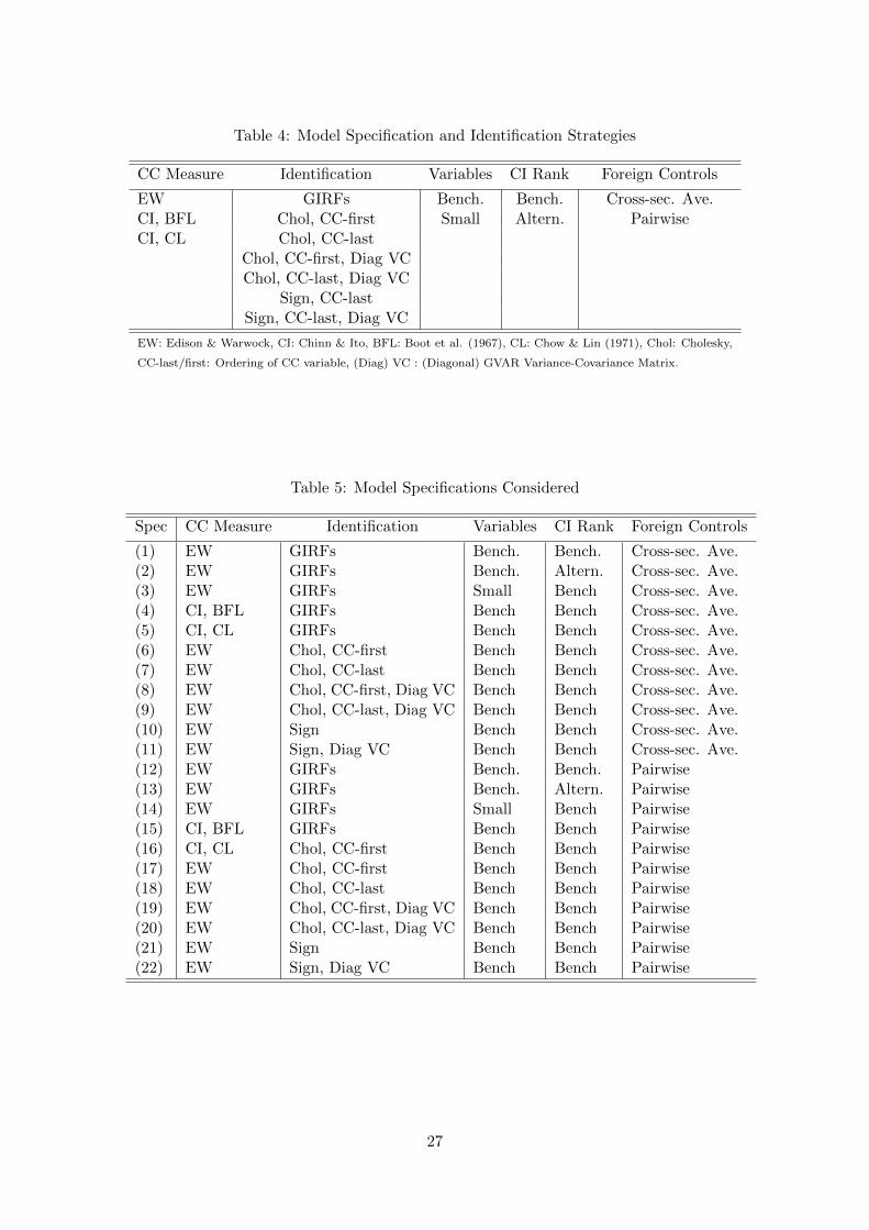
Table 4: Model Specification and Identification Strategies

CC Measure Identification Variables CI Rank Foreign Controls

EW GIRFs Bench. Bench. Cross-sec. Ave.CI, BFL Chol, CC-first Small Altern. PairwiseCI, CL Chol, CC-last

Chol, CC-first, Diag VCChol, CC-last, Diag VC

Sign, CC-lastSign, CC-last, Diag VC

EW: Edison & Warwock, CI: Chinn & Ito, BFL: Boot et al. (1967), CL: Chow & Lin (1971), Chol: Cholesky,

CC-last/first: Ordering of CC variable, (Diag) VC : (Diagonal) GVAR Variance-Covariance Matrix.

Table 5: Model Specifications Considered

Spec CC Measure Identification Variables CI Rank Foreign Controls

(1) EW GIRFs Bench. Bench. Cross-sec. Ave.(2) EW GIRFs Bench. Altern. Cross-sec. Ave.(3) EW GIRFs Small Bench Cross-sec. Ave.(4) CI, BFL GIRFs Bench Bench Cross-sec. Ave.(5) CI, CL GIRFs Bench Bench Cross-sec. Ave.(6) EW Chol, CC-first Bench Bench Cross-sec. Ave.(7) EW Chol, CC-last Bench Bench Cross-sec. Ave.(8) EW Chol, CC-first, Diag VC Bench Bench Cross-sec. Ave.(9) EW Chol, CC-last, Diag VC Bench Bench Cross-sec. Ave.(10) EW Sign Bench Bench Cross-sec. Ave.(11) EW Sign, Diag VC Bench Bench Cross-sec. Ave.(12) EW GIRFs Bench. Bench. Pairwise(13) EW GIRFs Bench. Altern. Pairwise(14) EW GIRFs Small Bench Pairwise(15) CI, BFL GIRFs Bench Bench Pairwise(16) CI, CL Chol, CC-first Bench Bench Pairwise(17) EW Chol, CC-first Bench Bench Pairwise(18) EW Chol, CC-last Bench Bench Pairwise(19) EW Chol, CC-first, Diag VC Bench Bench Pairwise(20) EW Chol, CC-last, Diag VC Bench Bench Pairwise(21) EW Sign Bench Bench Pairwise(22) EW Sign, Diag VC Bench Bench Pairwise

27

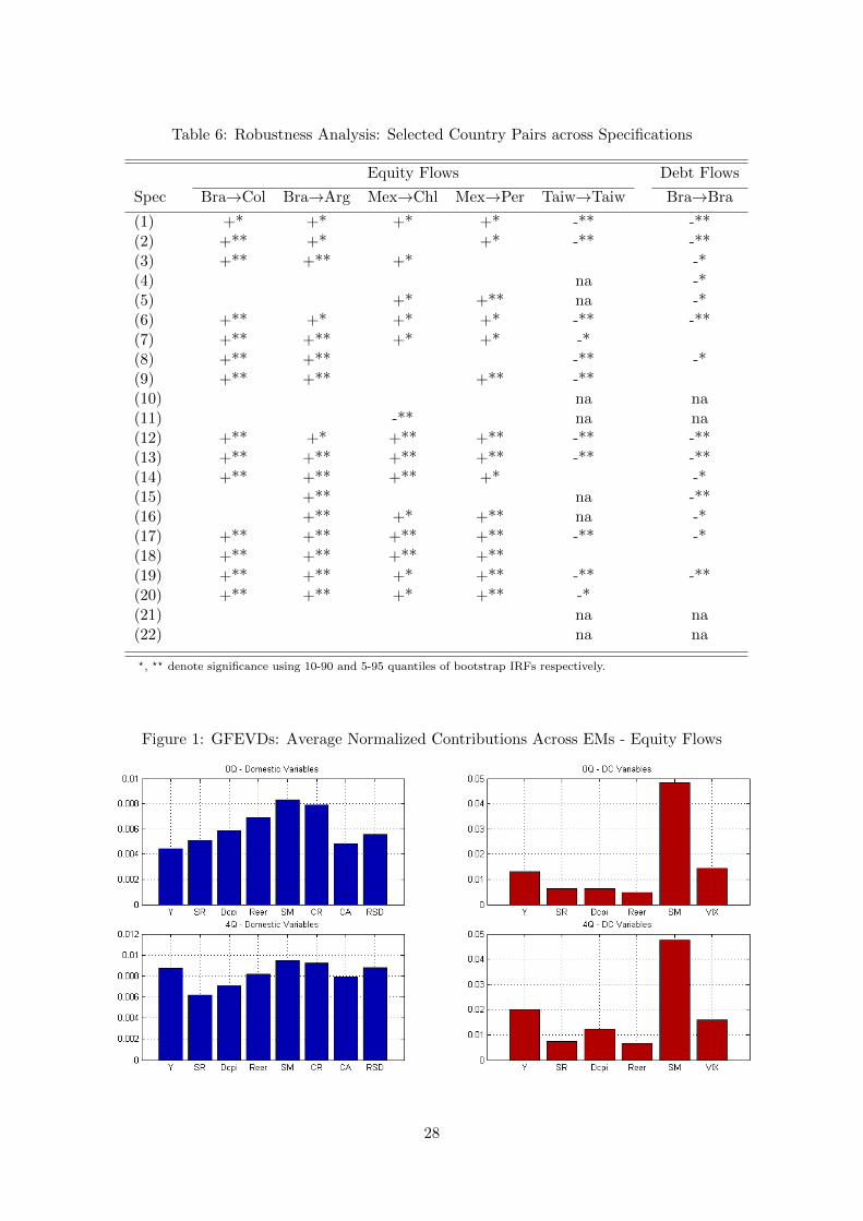
Table 6: Robustness Analysis: Selected Country Pairs across Specifications

Equity Flows Debt Flows

Spec Bra→Col Bra→Arg Mex→Chl Mex→Per Taiw→Taiw Bra→Bra

(1) +* +* +* +* -** -**(2) +** +* +* -** -**(3) +** +** +* -*(4) na -*(5) +* +** na -*(6) +** +* +* +* -** -**(7) +** +** +* +* -*(8) +** +** -** -*(9) +** +** +** -**(10) na na(11) -** na na(12) +** +* +** +** -** -**(13) +** +** +** +** -** -**(14) +** +** +** +* -*(15) +** na -**(16) +** +* +** na -*(17) +** +** +** +** -** -*(18) +** +** +** +**(19) +** +** +* +** -** -**(20) +** +** +* +** -*(21) na na(22) na na

?, ?? denote significance using 10-90 and 5-95 quantiles of bootstrap IRFs respectively.

Figure 1: GFEVDs: Average Normalized Contributions Across EMs - Equity Flows

28

Figure 2: GFEVDs: Fundamentals Contributions towards Equity Flows

Figure 3: GFEVDs: Total Contributions of Pull vs Push Factors

Figure 4: IRFs: Disaggregated Capital Controls Shocks for Selected Country Pairs

Lines in different colours represent IRFs under alternative specifications for given country pair.

29