modelling multivariate count data using copulas

HAL Id: hal-00537682https://hal.archives-ouvertes.fr/hal-00537682

Submitted on 19 Nov 2010

HAL is a multi-disciplinary open accessarchive for the deposit and dissemination of sci-entific research documents, whether they are pub-lished or not. The documents may come fromteaching and research institutions in France orabroad, or from public or private research centers.

L’archive ouverte pluridisciplinaire HAL, estdestinée au dépôt et à la diffusion de documentsscientifiques de niveau recherche, publiés ou non,émanant des établissements d’enseignement et derecherche français ou étrangers, des laboratoirespublics ou privés.

Modelling multivariate count data using copulasDimitris Karlis, Aristidis K. Nikoloulopoulos

To cite this version:Dimitris Karlis, Aristidis K. Nikoloulopoulos. Modelling multivariate count data using copulas. Com-munications in Statistics - Simulation and Computation, Taylor & Francis, 2009, 39 (01), pp.172-187.�10.1080/03610910903391262�. �hal-00537682�

https://hal.archives-ouvertes.fr/hal-00537682

https://hal.archives-ouvertes.fr

For Peer Review O

nly

Modelling multivariate count data using copulas

Journal: Communications in Statistics - Simulation and Computation

Manuscript ID: LSSP-2008-0315.R2

Manuscript Type: Original Paper

Date Submitted by the Author:

22-Sep-2009

Complete List of Authors: Karlis, Dimitris; Athens University of Economics, Statistics Nikoloulopoulos, Aristidis; University of East Anglia, Computing Sciences

Keywords: copulas, discrete distributions, super market data, archimedean

copulas

Abstract:

Multivariate count data occur in several different disciplines. However, existing models do not offer great flexibility for dependence modeling. Models based on copulas nowadays are widely used for continuous data dependence modeling. Modeling count data via copulas is still in its infancy; see the recent paper of Genest and Neshlehova (2007) A series of different copula models providing various residual dependence structures are considered for vectors of count response variables whose marginal

distributions depend on covariates through negative binomial regressions. A real data application related to the number of purchases of different products is provided.

Note: The following files were submitted by the author for peer review, but cannot be converted to PDF. You must view these files (e.g. movies) online.

LSSP-2008-0315.R2 Nikoloulopoulos and KArlis.zip

URL: http://mc.manuscriptcentral.com/lssp E-mail: [email protected]

Communications in Statistics - Simulation and Computation

For Peer Review O

nly

Page 1 of 23



123456789101112131415161718192021222324252627282930313233343536373839404142434445464748495051525354555657585960

For Peer Review O

nlyModeling multivariate count data using copulas

Aristidis K. Nikoloulopoulos ∗ Dimitris Karlis †

Abstract

Multivariate count data occur in several different disciplines. However, ex-isting models do not offer great flexibility for dependence modeling. Modelsbased on copulas nowadays are widely used for continuous data dependencemodeling. Modeling count data via copulas is still in its infancy; see therecent paper of Genest and Neslehova (2007). A series of different copulamodels providing various residual dependence structures are considered forvectors of count response variables whose marginal distributions depend oncovariates through negative binomial regressions. A real data applicationrelated to the number of purchases of different products is provided.

Keywords: Kendall’s tau; Archimedean copulas; partially symmetric copulas;

mixtures of max-id copulas; market basket count data.

1 Introduction

Multivariate count data occur in several disciplines, like epidemiology, marketing,

criminology, industrial statistics, among others. In marketing, modeling the num-

ber of purchases of different products has been of special interest as it has various

implications like predicting sales in the future, examining the behavior and the ty-

pology of buyers, creating marketing strategies, e.t.c. In addition, working jointly

with more products can be quite useful to derive new marketing strategies; see for

e.g., Brijs et al. (2004).

Accordingly, if only one product is considered then we loose valuable information

related to moving to different brands, using substitutes or finding related products

∗[email protected], School of Computing Sciences, University of East Anglia,

Norwich NR4 7TJ, UK†[email protected], Department of Statistics, Athens University of Economics and Business,

76 Patission street, 10434 Athens, Greece.

1

Page 2 of 23



123456789101112131415161718192021222324252627282930313233343536373839404142434445464748495051525354555657585960

For Peer Review O

nlythat are purchased together. Therefore, working with more products or with one

product but in successive time periods, allow us to reveal the existing structure in

the buying behavior and perhaps predict in a better way the expected income from

each customer; see Hoogendoorn and Sickel (1999). However, flexible models for

such data are not widely available and usually are hard to be fitted in real data.

Most of the existing models start from the multivariate Poisson model; see

Johnson et al. (1997). The multivariate Poisson distributions allows only for pos-

itive correlation. Typical extensions are based on mixtures (see for e.g., Chib and

Winkelmann (2001) and Karlis and Xekalaki (2005) and the references therein)

to allow for flexible correlation structure and overdispersed marginal distributions.

However, a certain limitation is that since the correlation structure comes from a

multivariate mixing distribution, the possible choices are very limited and perhaps

they lead to very specific marginal models. On the other hand models based on other

discrete distributions can be also constructed as for example the bivariate negative

binomial model of Winkelmann (2000) or models based on conditional distributions;

Berkhout and Plug (2004). Such models suffer from the difficulty to generalize to

other families of marginal distributions.

All the above usually have marginal distribution of a specific kind and the de-

pendence structure offered is limited. For this reason, we proceed by considering

the use of copula based models. The literature on copulas used for count data is

limited. We aim at contributing in this area by considering copula-based models for

multivariate counts that allow for both flexible dependence structure and flexible

marginal distributions. The specification in this way of the multivariate discrete

distribution provides complete inference, i.e., maximum likelihood estimation and

calculation of joint and conditional probabilities. The latter is not provided by other

methods such as log-linear models, see for e.g., Wedel et al. (2003), and generalized

estimating equations (GEE), see for e.g., Liang and Zeger (1986). The models de-

rived in the paper are based on known parametric families of copulas. However, to

our knowledge this is the first time of using some of them for count data dependence

modeling and their comparison reveals interesting implications on their use for real

data.

By definition, an m-variate copula C(u1, . . . , um) is a cumulative distribution

function (cdf) with uniform marginals on the interval (0, 1); see for e.g., Joe (1997)

or Nelsen (2006). If Fj(yj) is the cdf of a univariate random variable Yj, then

C(F1(y1), . . . , Fm(ym)) is an m-variate distribution for Y = (Y1, . . . , Ym) with marginal

distributions Fj, j = 1, . . . ,m. Conversely, if H is an m-variate cdf with univari-

2

Page 3 of 23



123456789101112131415161718192021222324252627282930313233343536373839404142434445464748495051525354555657585960

For Peer Review O

nlyate marginal cdfs F1, . . . , Fm, then there exists an m-variate copula C such for all

y = (y1, . . . , ym),

H(y1, . . . , ym) = C(F1(y1), . . . , Fm(ym)). (1)

If F1, . . . , Fm are continuous, then C is unique; otherwise, there are many possible

copulas as emphasized by Genest and Neslehova (2007), but all of these coincide

on the closure of Ran(F1) × · · · × Ran(Fm), where Ran(F ) denotes the range of F .

This result, known as Sklar’s theorem, indicates the way that multivariate cdfs and

their univariate cdfs can be connected. While the derivation of joint density is easy

for the continuous case through partial derivatives, it is not so simple in the case of

discrete data. In the latter case the probability mass function (pmf) h(·) is obtained

using finite differences as indicated in the following proposition:

Proposition 1.1. Consider a discrete integer-valued random vector (Y1, . . . , Ym)

with marginals F1, . . . , Fm and joint cdf given by the copula representation H(y1, . . . , ym) =

C(F1(y1), . . . , Fm(ym)). Let c = (c1, . . . , cm) be vertices where each ck is equal to ei-

ther yk or yk − 1, k = 1, . . . ,m. Then the joint pmf h(·) of the discrete random

variables Y1, . . . , Ym is given by

h(y1, y2, . . . , ym) =∑

sgn(c)C(F1(c1), . . . , Fm(cm)),

where the sum is taken over all vertices c, and sgn(c) is given by,

sgn(c) =

{1, if ck = yk − 1 for an even number of k’s.

−1, if ck = yk − 1 for an odd number of k’s.

From the above it is evident that for calculating the joint probability function, one

needs to evaluate the copula repeatedly. Therefore, in practice, in order to be able

to use copula models for multivariate count data, one needs to specify copulas with

computationally feasible form of the cdf.

Multivariate elliptical (for e.g., normal) copulas, see Fang et al. (2002) and Ab-

dous et al. (2005), provide flexible structure (allowing both positive and negative

dependence), but they do not have a closed form cdf. Therefore, computational

problems appear for m > 2 in the derivation of pmf which involves computation

of the copula in several different points and hence repeated multivariate numerical

integration. Van Ophem (1999) and Lee (2001) exploit the use of bivariate normal

copula to model count data, while Song (2000, 2007) defined multivariate disper-

sion models through multivariate normal copula. Computational problems for the

multivariate case are not mentioned, as the author concentrate his demonstration

3

Page 4 of 23



123456789101112131415161718192021222324252627282930313233343536373839404142434445464748495051525354555657585960

For Peer Review O

nlyon exchangeable dependence where multidimensional probabilities are 1-dimensional

integrals; Joe (1995).

The remaining literature for copulas and discrete data is concentrated to copulas

with a closed form cdf. There are few papers using Archimedean copulas with

discrete data; Meester and MacKay (1994), Lee (1999), Tregouet et al. (1999),

Cameron et al. (2004), and McHale and Scarf (2007). Therein Frank copula used

to model mainly bivariate discrete data (i.e. count and binary data), allowing both

positive and negative residual dependence. For multivariate data, Frank copula allow

only exchangeable structure with a narrower range of negative residual dependence

as the dimension increases; see for e.g., Joe (1997).

Joe (1993) defined the partially symmetric copulas extending Archimedean to a

class with a non-exchangeable structure. Zimmer and Trivedi (2006) and Paiva and

Kolev (2009) use a trivariate partially symmetric Frank copula to model discrete

data.

The pioneering work of Joe and Hu (1996) defining multivariate parametric fam-

ilies of copulas that are mixtures of max-id bivariate copulas has remained almost

completely overseen for modeling multivariate count data. Recently, Nikoloulopou-

los and Karlis (2008) predict dependent binary outcomes using this class of copulas,

which allows flexible dependence among the random variables and has a closed form

cdf and thus computations are rather easy. Herein we will present its superiority in

contrast with the other existing classes of copulas and propose its use for multivariate

count data modeling.

The remaining of the paper proceeds as follows: Section 2 presents briefly the

multivariate copula families with a closed form cdf, which will be used in this paper

in a self-contained manner. Section 3 describes how copula functions can be used to

model dependence on count data. In Section 4 estimation procedures are presented,

while in Section 5 a real data application, concerning market basket count data, is

provided. In fact, the copula functions are used to describe the dependence of error

terms in negative binomial regression models for marginals considered. Finally in

Section 6 concluding remarks can be found.

4

Page 5 of 23



123456789101112131415161718192021222324252627282930313233343536373839404142434445464748495051525354555657585960

For Peer Review O

nly2 Multivariate parametric families of copulas

2.1 Multivariate Archimedean copulas

Let Λ be a univariate cdf of a positive random variable (Λ(0) = 0), and let φ be the

Laplace transform (LT) of Λ,

φ(t) =

∫ ∞

0

e−tsdΛ(s), t ≥ 0,

For an arbitrary univariate cdf F , there exists a unique cdf G, such that

F (x) =

∫ ∞

0

Gs(x)dΛ(s) = φ(− log G(x)) (2)

directing to G(x) = exp (−φ−1(F (x))), where φ−1 is the functional inverse of φ.

Extending this result for bivariate case the following formula is a bivariate cdf,

∫ ∞

0

Gs1(y1)G

s2(y2)dΛ(s) = φ(− log G1(y1)−log G2(y2)) = φ

(φ−1(F1(y1)) + φ−1(F2(y2))

).

where now Gj(x) = exp (−φ−1(Fj(x))) , j = 1, 2. The bivariate copula

C(u1, u2) = φ(φ−1(u1) + φ−1(u2)), (3)

is the well known Archimedean copula with generator the inverse function of the

LT.

The multivariate Archimedean copula is a simple extension of (3) to the m-

variate case,

C(u) = φ

(m∑

j=1

φ−1(uj)

). (4)

This multivariate copula is permutation-symmetric in the m arguments, thus it is a

distribution for exchangeable U(0, 1) random variables with Kendall’s tau associa-

tion matrix,

1 τφ · · · τφ

......

......

τφ τφ · · · 1

.

One can see in the latter matrix that there is a common LT for all bivariate

marginals. Therefore, all pairs of variables have the same association, which is

rather restrictive in practice. Finally, as LTs one can use the choices LTA to LTD

in Table 1.

5

Page 6 of 23



123456789101112131415161718192021222324252627282930313233343536373839404142434445464748495051525354555657585960

For Peer Review O

nly2.2 Partially-symmetric copulas

Joe (1993) extended multivariate Archimedean copulas to a more flexible class of

copulas using nested LTs, the so called partially-symmetric m-variate copulas with

m − 1 dependence parameters. The multivariate form has a complex notation, so

we present the trivariate and 4-variate extensions of (4) to help the exposition. The

trivariate form is given by,

C(u) = φ1

(φ−1

1 ◦ φ2

(φ−1

2 (u1) + φ−12 (u2)

)+ φ−1

1 (u3)), (5)

where φ1, φ2 are LTs and φ−11 ◦ φ2 ∈ L⋆

∞ = {ω : [0,∞) −→ [0,∞)|ω(0) = 0, ω(∞) =

∞, (−1)j−1ωj ≥ 0, j = 1, . . . ,∞}. From the above formula is clear that (5) has (1,2)

bivariate margin of the form (3) with LT φ2, and (1,3), (2,3) bivariate margins of

the form (3) with LT φ1.

As the dimension increases there are many possible LT nestings. For the 4-

variate case the two possible LT nestings are,

C(u) = φ1

(φ−1

1 ◦ φ2

(φ−1

2 ◦ φ3

(φ−1

3 (u1) + φ−13 (u2)

)+ φ−1

2 (u3))

+ φ−11 (u4)

)(6)

C(u) = φ1

(φ−1

1 ◦ φ2

(φ−1

2 (u1) + φ−12 (u2)

)+ φ−1

1 ◦ φ3

(φ−1

3 (u3) + φ−13 (u4)

))(7)

where φ1, φ2, φ3 are LTs and φ−11 ◦φ2, φ

−11 ◦φ3 ∈ L⋆

∞ defined earlier. For the 4-variate

case of the forms (6) and (7) all the trivariate margins have form (5) and all the

bivariate have form (3). The Kendall’s tau association matrix for the copula given

in (5) is,

1 τφ2τφ1

τφ21 τφ1

τφ1τφ1

1

,

where τφ2> τφ1

.

In the same manner, the Kendall’s tau association matrix for the copula of the form

(6) is,

1 τφ3τφ2

τφ1

τφ31 τφ2

τφ1

τφ2τφ2

1 τφ1

τφ1τφ1

τφ11

,

where τφ1< τφ2

< τφ3, and the Kendall’s tau association matrix of the copula given

in (7) is,

1 τφ2τφ1

τφ1

τφ21 τφ1

τφ1

τφ1τφ1

1 τφ3

τφ1τφ1

τφ31

,

6

Page 7 of 23



123456789101112131415161718192021222324252627282930313233343536373839404142434445464748495051525354555657585960

For Peer Review O

nlywhere τφ1

< τφ2, τφ3

.

From the above one can realize that bivariate copulas associated with LTs that

are more nested, are larger in concordance than those that are less nested. For ex-

ample, for (7) the (1,2) and (3,4) bivariate margins are more dependent (concordant)

than the remaining four bivariate margins.

To make these results applicable some choices of LTs, in which the property

φ−11 ◦φ2 ∈ L⋆

∞, is satisfied are LTA to LTD (see Table 1). Note in passing that there

are still restrictions on the dependence structure allowed by such copulas and the

Archimedean copula is a subcase of partially symmetric copula when all LTs are

from the same family.

Table 1 about here

2.3 Copulas via mixtures of max-id bivariate copulas

Joe and Hu (1996) considered the mixture of univariate cdfs Hj and max-id bivariate

copulas C ′jk of the form

∫ ∞

0

∏

1≤j<k≤m

C′sjk(Hj, Hk)

m∏

j=1

Hνjsj dΛ(s)

= φ

(−

∑

1≤j<k≤m

log C ′jk(Hj, Hk) +

m∑

j=1

νj log Hj

). (8)

The above representation defines a multivariate copula if Hj are chosen appropri-

ately. The univariate margins of (8) are Fj = φ (−(νj + m − 1) log Hj), so substitut-

ing Hj(uj) = e−pjφ−1(uj) and pj = (νj +m−1)−1, j = 1, . . . ,m in (8) is a multivariate

copula distribution with a closed form cdf,

C(u) = φ

(−∑

j<k

log C ′jk(e−pjφ−1(uj), e−pkφ−1(uk)) +

m∑

j=1

νjpjφ−1(uj)

). (9)

It is well known that the mixing operation introduces dependence, so this new copula

has a dependence structure that comes from the form of C ′jk and the form of the

mixing distribution Λ(·) which is characterized by its LT φ(·).

Another interesting interpretation is that the LT φ introduces the minimal de-

pendence between the random variables, while the copulas C ′jk provide some addi-

tional pairwise dependence beyond the minimal dependence. The parameters νj are

included in order that the parametric family of multivariate copulas (9) is closed

7

Page 8 of 23



123456789101112131415161718192021222324252627282930313233343536373839404142434445464748495051525354555657585960

For Peer Review O

nlyunder margins. Taking, Hr −→ 1,∀r ∈ {1, . . . ,m} \ {j, k} in (8) the (j, k) bivariate

marginal copula of (9) is,

Cjk(uj, uk) = φ(− log C ′

jk(e−pjφ−1(uj), e−pkφ−1(uk)) +

+(νj + m − 2)piφ−1(ui) + (νk + m − 2)pkφ

−1(uk)). (10)

Keeping νj as known parameters, the copula of the form (9) is a family with m(m−1)2

+

1 parameters with flexible dependence. One may simplify the form of the copula

by assuming C ′rs(ur, us) = urus (product copula, independence) together with νr =

νs = −1, for some pairs. This implies that for that pairs of variables we assume

the minimum level of dependence as introduced by φ. This allows to simplify the

model and reduce the number of parameters to be estimated. Note in passing that

the model in its full form allows for different association for each pair of variables.

Some of the choices of bivariate max-id copulas are Galambos, Gumbel, Frank,

Joe, and Mardia-Takahasi (also known as Clayton or Kimeldorf-Sampson copula).

These, together with some LT can be seen in Table 1 (LTA to LTD). Their combina-

tion results in a variety of parametric families of the form (9) with flexible positive

dependence structure. Of course this provides a rich pool of candidate models and

deserves some model selection technique. Note that we can construct multivariate

copulas that are mixtures of common C ′jk(·) = C ′(·; θjk) and not common max-id

copulas to provide the most flexible dependence according to data on hand.

2.4 Negative dependence

As we have already mention multivariate Archimedean copulas provide a narrower

range of dependence as the dimension increases, see also McNeil and Neslehova

(2009) for a thorough treatment. Furthermore partially symmetric and mixtures

of max-id copulas provide only positive dependence by definition, see Joe (1997).

What about if the data on hand have negative dependence?

Negative dependence can be introduced by applying decreasing transformations

to the oppositely ordered variables. If (U1, . . . , Um) ∼ C where C is a copula with

positive dependence, one could always get some negative dependence for a subset of

variables, by supposing C∗ is the copula of (U1, . . . , Uk, 1 − Uk+1, . . . , 1 − Um).

8

Page 9 of 23



123456789101112131415161718192021222324252627282930313233343536373839404142434445464748495051525354555657585960

For Peer Review O

nly3 Copulas and Dependence for count data

The dependence between random variables is completely described by their joint

distribution, which can be represented by (1). For continuous random variables,

dependence as measured by Kendall’s tau (τ) is associated only with the copula

parameters; see for e.g., Nelsen (2006). This is, however, not the case for discrete

data because the probability of a tie is positive; see Denuit and Lambert (2005),

Mesfioui and Tajar (2005). For this reason the marginal distributions play also some

role on dependence, and τ does not attain ±1 values. Here, we provide a formula

for Kendall’s tau; see Nikoloulopoulos (2007) for the derivation. For normalized

versions one can refer to Goodman and Kruskal (1954) or Neslehova (2007).

Lemma 3.1. Let Yi, i = 1, 2 be integer-valued discrete random variables whose joint

distribution is H, with marginal cdfs Fi, pmfs fi, i = 1, 2 and copula C. Then the

population version of Kendall’s tau for Y1 and Y2 is given by

τ(Y1, Y2) =∞∑

y1=0

∞∑

y2=0

h(y1, y2){4C(F1(y1 − 1), F2(y2 − 1)) − h(y1, y2)} +

∞∑

y1=0

(f 2

1 (y1) + f 22 (y1)

)− 1, (11)

where,

h(y1, y2) = C(F1(y1), F2(y2)) − C(F1(y1 − 1), F2(y2))

− C(F1(y1), F2(y2 − 1)) + C(F1(y1 − 1), F2(y2 − 1))

is the joint pmf of Y1 and Y2.

This representation of Kendall’s tau is equivalent to the one derived in Denuit and

Lambert (2005). In fact it provides us with better insight, since the marginal prob-

ability functions fi, i = 1, 2 are clearly involved in the formulas and make clear the

dependence of Kendall’s tau on the marginal distributions.

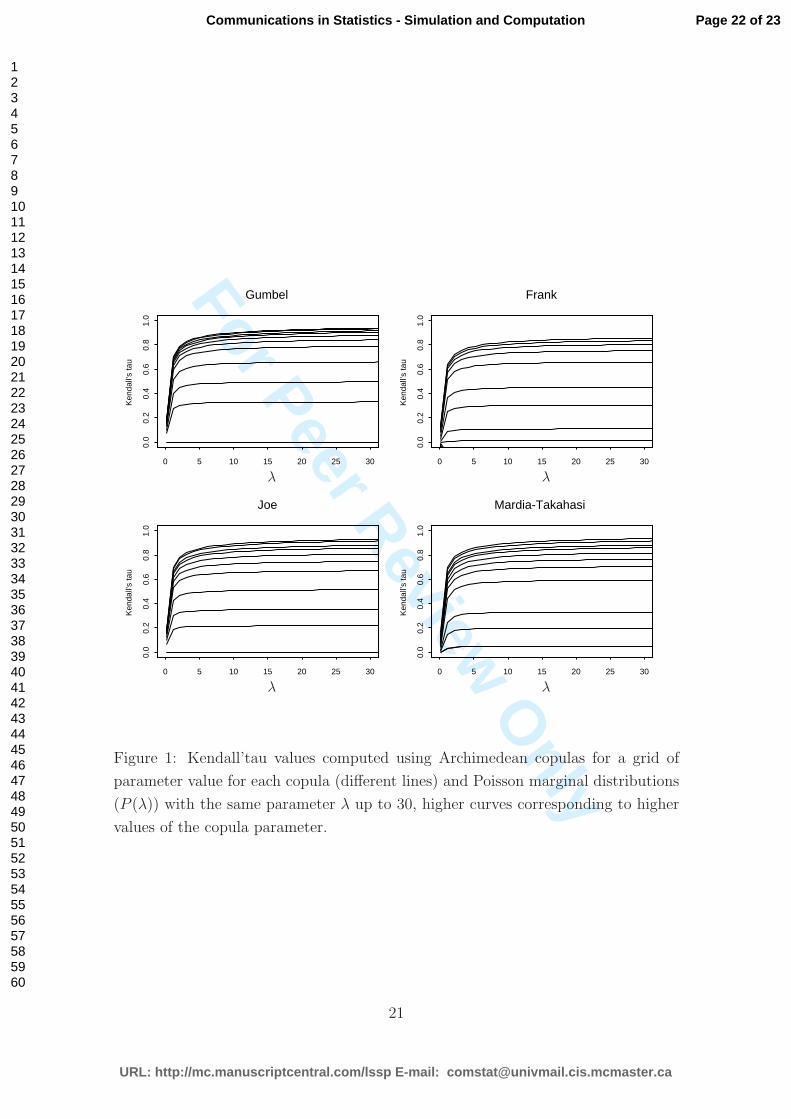
In Figure 1 Kendall’s tau values have been plotted for Archimedean copulas (for

each copula the lines correspond to different values of its parameter). We have used

Poisson marginal distributions with the same parameter for each marginal. The plot

depicts Kendall’tau values against this common Poisson parameter. Higher curves

corresponding to higher values of the copula parameter.

From the plot we can see that for marginal parameters (denoted by λ) greater

than 10 their association with the value of Kendall’s tau is negligible. Moreover as

λ tends to infinity, the upper bound of Kendall’s tau is 1, due to absence of ties.

9

Page 10 of 23



123456789101112131415161718192021222324252627282930313233343536373839404142434445464748495051525354555657585960

For Peer Review O

nlyFigure 1 about here

4 Estimation of a multivariate copula based model

Consider a multivariate copula based parametric model for the random vector y

with m elements and distribution function H provided by the copula representation

H(y; α1, . . . , αm, θ) = C(F1(y1; α1), . . . , Fm(ym; αm); θ), (12)

where Fi are the marginal cdfs, with parameter vectors αi, i = 1, . . . ,m and θ is the

vector of copula parameter. The pmf h(y; α1, . . . , αm, θ) of the specified cdf H in

(12) can be obtained using Proposition 1.1.

Consider the m log-likelihoods functions for the univariate marginal distribu-

tions:

Lyj(αj) =

n∑

i=1

log fj(yij; αj), j = 1, . . . ,m (13)

and the joint log-likelihood

L(θ, α1, . . . , αm) =n∑

i=1

log h(yi1, . . . , yim; α1, . . . , αm, θ), (14)

where fi, i = 1, . . . ,m are the marginal pmfs and n is the sample size.

Efficient estimation of the model parameters is succeeded by the inference func-

tion of margins (IFM), which consists of a two step approach. At the first step of

this method the univariate log-likelihoods (13) are maximized independently of the

copula parameter and at the second step the joint log-likelihood (14) maximized

over θ with univariate parameters fixed as estimated at the first step of the method.

Estimation by IFM method becomes more popular as the dimension increases and

computational problems arise. The problem of fitting multivariate data is decom-

posed into two smaller problems: fitting the marginal distributions separately from

fitting the existing dependence structure. Asymptotic efficiency of the IFM has been

studied by Joe (2005) for a number of multivariate models. All of these compar-

isons suggest that the IFM method is highly efficient compared to FML, except for

extreme cases near the Frechet bounds.

10

Page 11 of 23



123456789101112131415161718192021222324252627282930313233343536373839404142434445464748495051525354555657585960

For Peer Review O

nly5 Application

5.1 The Data

Transactional market basket data provide excellent opportunities for a retailer to

segment the customer population into different groups based on differences in their

purchasing behavior. The data refer to the frequency of purchases of products or

product categories within the retail store and, as a result, they are extremely useful

for modeling consumer purchase behavior. Moreover they reflect the dependencies

that exist between purchases in different product categories.

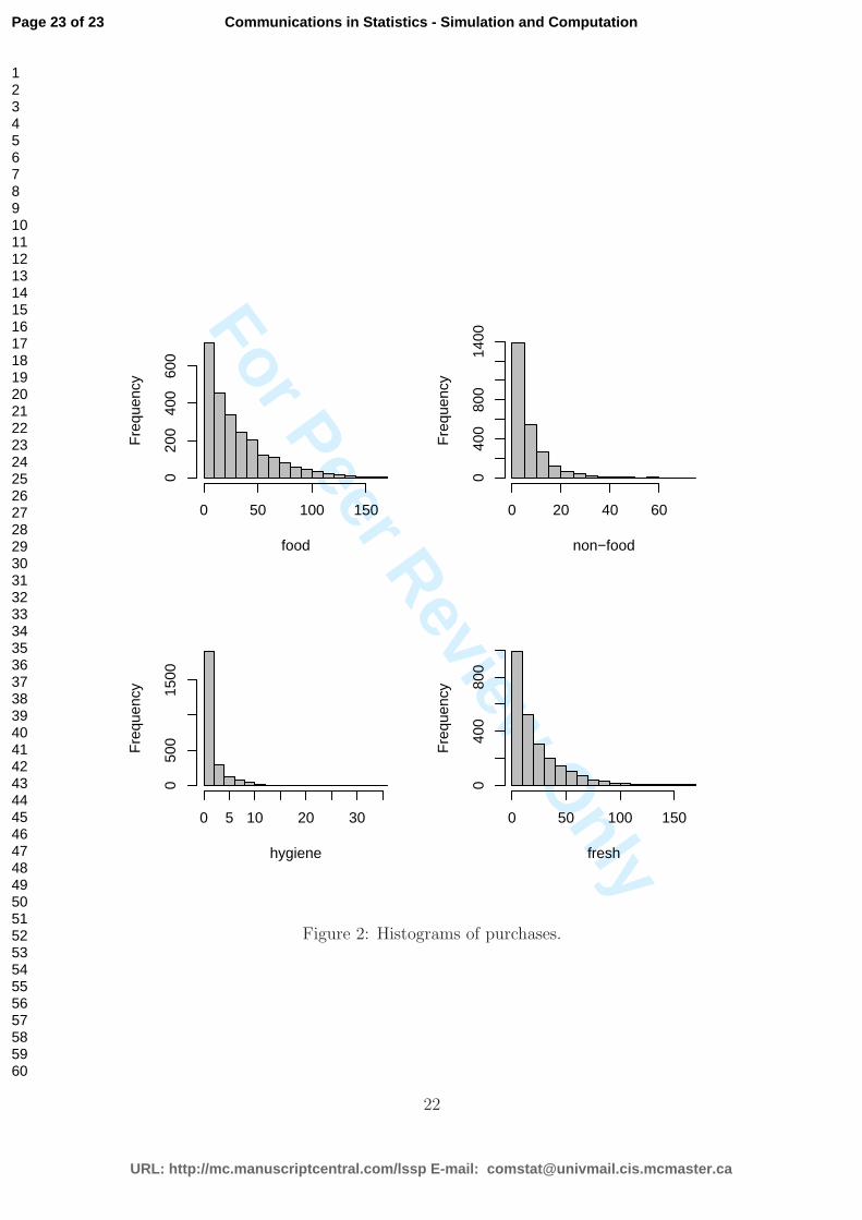
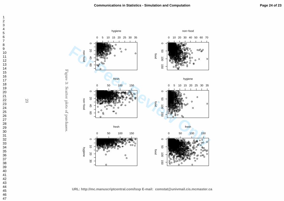
We used the scanner data in Brijs et al. (1999). The data refer to the number

of food, non-food, hygiene, and fresh purchases from loyalty card holders of a large

super market for a given month time period in Belgium. Hygiene category contains

articles like hair, gel, shaving foam, bath foam, toilet soap e.t.c., while fresh category

contains vegetables, fruit, meat, cheese and bakery items. It is a special category

because it contains all the food items that are not prepacked but are served by

personnel behind a counter. In Figure 2 and in Figure 3 one can see the large tails

and the present dependence on the data, respectively.

The use of copulas allows to specify the marginal distributions in a more flexible

way as we do not need to specify the entire model at once and hence the marginal

distributions can be selected separately. This can help considerably on selecting

improved models even with different marginal distributions.

Figures 2 and 3 about here

Therefore, before choosing the appropriate copula family to capture the de-

pendence between the residuals of the marginal model we specify the univariate

marginal distributions. For our data, the negative binomial model (see for e.g.,

Lawless (1987)) is considered, allowing for the large over-dispersion found in the

data. For each observation i = 1, . . . , 2472, each marginal is specified conditional

on covariates Xi and cumulative probability function given by

Fj(yij|Xi, βj) =

yij∑

k=0

Γ(σj + k)

Γ(σj)Γ(k + 1)

µkijσ

σj

j

(µij + σj)σj+k, i = 1, . . . , 2472 j = 1, 2, 3, 4 ,

(15)

where E(yij) = µij = exp(Xiβj) and var(yij) = µij + µ2ij/σj. A similar approach is

used by Cameron et al. (2004) and Paiva and Kolev (2009). The covariate informa-

tion refers to if the customers use their car to go for shopping in the supermarket, if

11

Page 12 of 23



123456789101112131415161718192021222324252627282930313233343536373839404142434445464748495051525354555657585960

For Peer Review O

nlythey have pets, if they have freezer, if they have microwave, and if they have garden

in their home. Moreover, the number of members of the family belonging to four

different age subcategories: (a) 0-18 years, (b) 18-45 years, (c) 45-65 years, and (d)

more than 65 years, was recorded to account for the household composition.

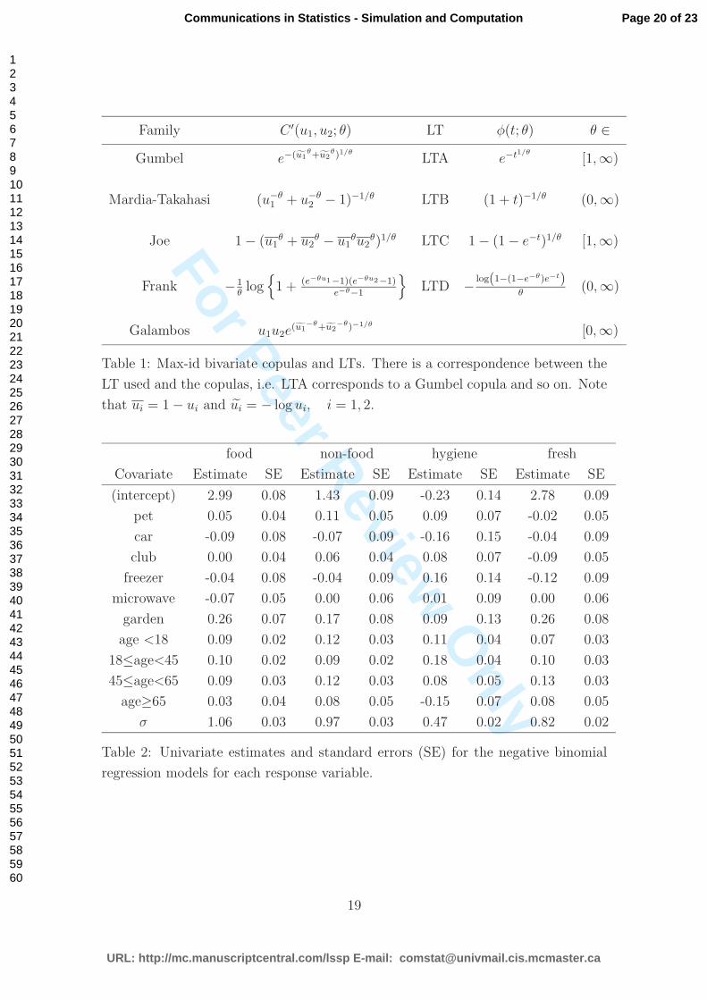
The univariate regression parameters, which estimated at the first step of the

IFM method, fitting separate negative binomial regression models for each response

variable, are shown in Table 2. As a preliminary data analysis we calculated the

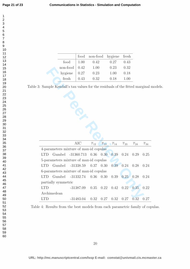
sample Kendall’s tau values for the residuals of the fitted marginal models, see Table

3. Greater dependence existed between food and non-food data and between food

and fresh data, while the lowest between hygiene and fresh data. For the remaining

marginals the strength of residual dependence was quite the average of lowest and

greater dependence and at quite the similar strength between purchases.

Tables 2 and 3 about here

5.2 4-variate fitted models

We started our modeling by considering the simplest structure provided by mul-

tivariate Archimedean copulas. This class assumes the same residual dependence

for each pair. Then we fitted partially symmetric copulas, see subsection 2.2, and

particularly the LT nesting given by (6) with some reordering of the uj’s to capture

the dependence in our data, i.e.,

C(u) = φ1

(φ−1

1 ◦ φ2

(φ−1

2 ◦ φ3

(φ−1

3 (u1) + φ−13 (u4)

)+ φ−1

2 (u2))

+ φ−11 (u3)

).

The Kendall’s tau correlation matrix for the copula of this form is,

1 τφ2τφ1

τφ3

τφ21 τφ1

τφ2

τφ1τφ1

1 τφ1

τφ3τφ2

τφ11

,

where τφ1< τφ2

< τφ3.

The next step was to fit copulas that are mixtures of max-id copulas of the

form (9) with seven dependence parameters, one for the LT (θ) and one (θjk) for

each marginal (j, k) keeping ν’s fixed and zero. Note here that one parameter is

redundant. Finally, based on preliminary data analysis (Table 3), we simplified the

models and numerical computations setting C ′34 = Π (independence copula) and

ν3 = ν4 = −1. In this manner we assumed a lower level of dependence for the

12

Page 13 of 23



123456789101112131415161718192021222324252627282930313233343536373839404142434445464748495051525354555657585960

For Peer Review O

nly(3,4) bivariate margin represented by the parameter θ of the LT φ and a higher

dependence for the other bivariate margins with the parameters θjk representing

bivariate dependence exceeding the minimum dependence of the LT φ.

5.3 Results

We fitted all copula-based models considered in the previous section using negative

binomial regression models for the margins. For each class of copulas, several families

are considered by choosing different LTs and/or max-id copulas. Table 4 provides

the best model for each class, summarizing our findings.

Table 4 about here

To compare the models we report the AIC, which was calculated as the max-

imized log-likelihood minus the number of model parameters, to account for the

different number of parameters that each type of models has. In addition, we report

the average Kendall’s tau values for each pair of variables to account for the strength

of the residual dependence imposed among purchases.

There are some interesting findings from Table 4. Starting from the simpler

model, the multivariate Archimedean copulas, which offer only exchangeable residual

dependence, the results contradict with the data and thus they provide the worst

AIC. Remember here that for count data with small mean values the Kendall’s tau is

associated both with marginal and copula parameters, see Figure 1. To this end, the

reason for the lower residual dependence on marginals (1,3), (2,3), and (3,4) is due

to the fact that hygiene response has small mean value. The next most complicated

model, the partially symmetric copulas, with three copula parameters, provide more

flexibility and therefore better fit than Archimedean copulas.

Finally, the 6-parameters mixture of max-id copulas are better from the partially

symmetric copulas, because they provide flexible residual dependence, meaning that

the number of bivariate marginals is equal to the number of dependence parame-

ters. Note that more parsimonious models also fitted by removing parameters with

estimated values near the boundary of the parameter space, and assuming prod-

uct copulas for these pairs of variables. While such models involve less parameters

we found that the AIC value was worst than the 6-parameters mixture of max-id

copulas, as one can read in Table 4.

13

Page 14 of 23



123456789101112131415161718192021222324252627282930313233343536373839404142434445464748495051525354555657585960

For Peer Review O

nly5.4 Managerial implications

We briefly mention in this subsection the interesting findings from the managerial

point of view. First of all probabilities of any kind can be easily obtained based on

Proposition 1.1. Thus one can easily check for non-buyers, i.e. persons that will

not buy any of the products. Secondly for a new customer one may calculate the

expectation of purchases for each product category and hence deriving the expected

amount to be spent by this new customer. Such numbers can be quite helpful

for decision making. In addition the cross products correlations help to examine

effective marketing strategies by putting, for example, together products with large

correlation in order to promote them. Note also that conditional probabilities and

expectations can be deduced by simple calculus and thus predictions for joint number

of purchases can be made. The models presented are quite flexible and relatively

easy to apply with real data in order to facilitate such decisions. We do not pursue

further this issue on the present paper.

6 Concluding remarks

Modeling multivariate count data based on copulas was described in the present

paper. We presented and fitted a series of different multivariate copulas of varying

dependence structure indicating the importance of mixtures of max-id copulas in

terms of flexibility. We showed how to account for residual dependence among

count responses, given the explanatory variables. In our illustration the data were

positively associated, but generally real multivariate discrete data exist with some

negative associations, see for e.g., the cases in Aitchinson and Ho (1989) and Chib

and Winkelmann (2001). From the latter class, as we have mentioned one could

always get some negative dependence by applying decreasing transformations on

some subset of the random variables but this is restrictive in general, because this

construction cannot model negative dependence among many random variables.

The multivariate elliptical copulas inherit the dependence structure of ellipti-

cal distributions, i.e., allow for negative dependence, but lack a closed form cdf;

this means likelihood inference might be difficult as multidimensional integration is

required for the multivariate probabilities.

Ongoing research is focused on defining a new multivariate parametric family of

copulas with computationally feasible form of the cdf and a wide range of depen-

dence, see for e.g., in Nikoloulopoulos and Karlis (2009).

14

Page 15 of 23



123456789101112131415161718192021222324252627282930313233343536373839404142434445464748495051525354555657585960

For Peer Review O

nlyAcknowledgements

This work is part of first author’s Ph.D. thesis under the supervision of the second

author at the Athens University of Economics and Business. The first author would

like to thank the National Scholarship Foundation of Greece for financial support.

The authors want to thank a referee for his constructive comments.

References

Abdous, B., Genest, C., and Remillard, B. (2005). Dependence properties of meta-

elliptical distributions. In Statistical modelling and analysis for complex data

problems, pages 1–15, Dordrecht, The Netherlands. Kluwer. (P. Duchesne &

Remillard, eds.).

Aitchinson, J. and Ho, C. (1989). The multivariate Poisson-log normal distribution.

Biometrika, 75:621–629.

Berkhout, P. and Plug, E. (2004). A bivariate Poisson count data model using

conditional probabilities. Statistica Neerlandica, 58:349–364.

Brijs, T., Karlis, D., Swinnen, G., Vanhoof, K., Wets, G., and Manchanda, P. (2004).

A multivariate Poisson mixture model for marketing applications. Statistica Neer-

landica, 58(3):322–348.

Brijs, T., Swinnen, G., Vanhoof, K., and Wets, G. (1999). Using association rules for

product assortment decisions: A case study. In Knowledge Discovery and Data

Mining, pages 254–260.

Cameron, A. C., Li, T., Trivedi, P. K., and Zimmer, D. M. (2004). Modelling the

differences in counted outcomes using bivariate copula models with application

to mismeasured counts. The Econometrics Journal, 7(2):566–584.

Cameron, A. C. and Trivedi, P. K. (1998). Regression Analysis of Count Data.

Cambridge University Press, Cambridge.

Chib, S. and Winkelmann, R. (2001). Markov chain Monte Carlo analysis of corre-

lated count data. Journal of Business & Economic Statistics, 19(4):428–435.

Denuit, M. and Lambert, P. (2005). Constraints on concordance measures in bivari-

ate discrete data. Journal of Multivariate Analysis, 93(1):40–57.

15

Page 16 of 23



123456789101112131415161718192021222324252627282930313233343536373839404142434445464748495051525354555657585960

For Peer Review O

nlyFang, H.-B., Fang, K.-T., and Kotz, S. (2002). The meta-elliptical distributions

with given marginals. Journal of Multivariate Analysis, 82:1–16.

Genest, C. and Neslehova, J. (2007). A primer on copulas for count data. The Astin

Bulletin, 37:475–515.

Goodman, L. and Kruskal, W. (1954). Measures of association for cross classifica-

tions. Journal of the American Statistical Association, 49:732764.

Hoogendoorn, A. W. and Sickel, D. (1999). Description of purchase incidence by

multivariate heterogeneous Poisson processes. Statistica Neerlandica, 53(1):21–35.

Joe, H. (1993). Parametric families of multivariate distributions with given margins.

Journal of Multivariate Analysis, 46:262–282.

Joe, H. (1995). Approximations to multivariate normal rectangle probabilities based

on conditional expectations. Journal of the American Statistical Association,

90(431):957–964.

Joe, H. (1997). Multivariate Models and Dependence Concepts. Chapman & Hall,

London.

Joe, H. (2005). Asymptotic efficiency of the two-stage estimation method for copula-

based models. Journal of Multivariate Analysis, 94(2):401–419.

Joe, H. and Hu, T. (1996). Multivariate distributions from mixtures of max-infinitely

divisible distributions. Journal of Multivariate Analysis, 57(2):240–265.

Johnson, N., Kotz, S., and Balakrishnan, N. (1997). Discrete Multivariate Distribu-

tions. Wiley, New York.

Karlis, D. and Xekalaki, E. (2005). Mixed Poisson distributions. International

Statistical Review, 73:35–58.

Lawless, J. F. (1987). Negative binomial and mixed Poisson regression. The Cana-

dian Journal of Statistics, 15(3):209–225.

Lee, A. (1999). Modelling rugby league data via bivariate negative binomial regres-

sion. Australian and New Zealand Journal of Statistics, 41(2):141–152.

Lee, L.-F. (2001). On the range of correlation coefficients of bivariate ordered discrete

random variables. Econometric Theory, 17(1):247–256.

16

Page 17 of 23



123456789101112131415161718192021222324252627282930313233343536373839404142434445464748495051525354555657585960

For Peer Review O

nlyLiang, K. and Zeger, S. (1986). Longitudinal data analysis using generalized linear

models. Biometrika, 73:13–22.

McHale, I. and Scarf, P. (2007). Modelling soccer matches using bivariate dis-

crete distributions with general dependence structure. Statistica Neerlandica,

61(4):432–445.

McNeil, A. J. and Neslehova, J. (2009). Multivariate Archimedean copulas, d-

monotone functions and l1-norm symmetric distributions. Annals of Statistics,

37:3059–3097.

Meester, S. and MacKay, J. (1994). A parametric model for cluster correlated

categorical data. Biometrics, 50:954–963.

Mesfioui, M. and Tajar, A. (2005). On the properties of some nonparametric con-

cordance measures in the discrete case. Journal of Nonparametric Statistics,

17(5):541–554.

Nelsen, R. B. (2006). An Introduction to Copulas. Springer-Verlag, New York.

Neslehova, J. (2007). On rank correlation measures for non-continuous random

variables. Journal of Multivariate Analysis, 98:544–567.

Nikoloulopoulos, A. K. (2007). Application of Copula Functions in Statistics. Ph.D.

thesis, Department of Statistics, Athens University of Economics.

Nikoloulopoulos, A. K. and Karlis, D. (2008). Multivariate logit copula model with

an application to dental data. Statistics in Medicine, 27:6393–6406.

Nikoloulopoulos, A. K. and Karlis, D. (2009). Finite normal mixture copulas for

multivariate discrete data modeling. Journal of Statistical Planning and Inference,

139:3878–3890.

Paiva, D. and Kolev, N. (2009). Copula-based regression models: A survey. Journal

of Statistical Planning and Inference, 139(11):3847–3856.

Song, P. X.-K. (2000). Multivariate dispersion models generated from Gaussian

copula. Scandinavian Journal of Statistics, 27(2):305–320.

Song, P. X.-K. (2007). Correlated Data Analysis: Modeling, Analytics, and Appli-

cation. Spinger, NY.

17

Page 18 of 23



123456789101112131415161718192021222324252627282930313233343536373839404142434445464748495051525354555657585960

For Peer Review O

nlyTregouet, D. A., Ducimetiere, P., Bocquet, V., Visvikis, S., Soubrier, F., and Tiret,

L. (1999). A parametric copula model for analysis of familial binary data. Amer-

ican Journal of Human Genetics, 64(3):886–93.

Van Ophem, H. (1999). A general method to estimate correlated discrete random

variables. Econometric Theory, 15(2):228–237.

Wedel, M., Bockenholt, U., and Kamakura, W. (2003). Factor models for multivari-

ate count data. Journal of Multivariate Analysis, 87:356–369.

Winkelmann, R. (2000). Seemingly unrelated negative binomial regression. Oxford

Bulletin of Economics and Statistics, 62(4):553–560.

Zimmer, D. and Trivedi, P. (2006). Using trivariate copulas to model sample selec-

tion and treatment effects: Application to family health care demand. Journal of

Business & Economic Statistics, 24(1):63–76.

18

Page 19 of 23



123456789101112131415161718192021222324252627282930313233343536373839404142434445464748495051525354555657585960

For Peer Review O

nlyFamily C ′(u1, u2; θ) LT φ(t; θ) θ ∈

Gumbel e−(u1θ+u2

θ)1/θLTA e−t1/θ

[1,∞)

Mardia-Takahasi (u−θ1 + u−θ

2 − 1)−1/θ LTB (1 + t)−1/θ (0,∞)

Joe 1 − (u1θ + u2

θ − u1θu2

θ)1/θ LTC 1 − (1 − e−t)1/θ [1,∞)

Frank −1θ

log{

1 + (e−θu1−1)(e−θu2−1)e−θ−1

}LTD −

log(1−(1−e−θ)e−t)θ

(0,∞)

Galambos u1u2e(u1

−θ+u2−θ)−1/θ

[0,∞)

Table 1: Max-id bivariate copulas and LTs. There is a correspondence between the

LT used and the copulas, i.e. LTA corresponds to a Gumbel copula and so on. Note

that ui = 1 − ui and ui = − log ui, i = 1, 2.

food non-food hygiene fresh

Covariate Estimate SE Estimate SE Estimate SE Estimate SE

(intercept) 2.99 0.08 1.43 0.09 -0.23 0.14 2.78 0.09

pet 0.05 0.04 0.11 0.05 0.09 0.07 -0.02 0.05

car -0.09 0.08 -0.07 0.09 -0.16 0.15 -0.04 0.09

club 0.00 0.04 0.06 0.04 0.08 0.07 -0.09 0.05

freezer -0.04 0.08 -0.04 0.09 0.16 0.14 -0.12 0.09

microwave -0.07 0.05 0.00 0.06 0.01 0.09 0.00 0.06

garden 0.26 0.07 0.17 0.08 0.09 0.13 0.26 0.08

age <18 0.09 0.02 0.12 0.03 0.11 0.04 0.07 0.03

18≤age<45 0.10 0.02 0.09 0.02 0.18 0.04 0.10 0.03

45≤age<65 0.09 0.03 0.12 0.03 0.08 0.05 0.13 0.03

age≥65 0.03 0.04 0.08 0.05 -0.15 0.07 0.08 0.05

σ 1.06 0.03 0.97 0.03 0.47 0.02 0.82 0.02

Table 2: Univariate estimates and standard errors (SE) for the negative binomial

regression models for each response variable.

19

Page 20 of 23



123456789101112131415161718192021222324252627282930313233343536373839404142434445464748495051525354555657585960

For Peer Review O

nlyfood non-food hygiene fresh

food 1.00 0.42 0.27 0.43

non-food 0.42 1.00 0.23 0.32

hygiene 0.27 0.23 1.00 0.18

fresh 0.43 0.32 0.18 1.00

Table 3: Sample Kendall’s tau values for the residuals of the fitted marginal models.

AIC τ 12 τ 13 τ 14 τ 23 τ 24 τ 34

4-parameters mixture of max-id copulas

LTD Gumbel -31360.713 0.36 0.30 0.39 0.24 0.29 0.25


LTD Gumbel -31338.59 0.37 0.30 0.39 0.24 0.28 0.24


LTD Gumbel -31332.74 0.36 0.30 0.39 0.25 0.28 0.24

partially symmetric

LTD -31387.09 0.35 0.22 0.42 0.22 0.35 0.22

Archimedean

LTD -31483.04 0.32 0.27 0.32 0.27 0.32 0.27

Table 4: Results from the best models from each parametric family of copulas.

20

Page 21 of 23



123456789101112131415161718192021222324252627282930313233343536373839404142434445464748495051525354555657585960

For Peer Review O

nlyGumbel

Ken

dall’

s ta

u

0 5 10 15 20 25 30

0.0

0.2

0.4

0.6

0.8

1.0

Frank

Ken

dall’

s ta

u

0 5 10 15 20 25 30

0.0

0.2

0.4

0.6

0.8

1.0

Joe

Ken

dall’

s ta

u

0 5 10 15 20 25 30

0.0

0.2

0.4

0.6

0.8

1.0

Mardia-Takahasi

Ken

dall’

s ta

u

0 5 10 15 20 25 30

0.0

0.2

0.4

0.6

0.8

1.0

λλ

λλ

Figure 1: Kendall’tau values computed using Archimedean copulas for a grid of

parameter value for each copula (different lines) and Poisson marginal distributions

(P (λ)) with the same parameter λ up to 30, higher curves corresponding to higher

values of the copula parameter.

21

Page 22 of 23



123456789101112131415161718192021222324252627282930313233343536373839404142434445464748495051525354555657585960

For Peer Review O

nly

food

Fre

quen

cy

0 50 100 150

020

040

060

0

non−food

Fre

quen

cy

0 20 40 60

040

080

014

00

hygiene

Fre

quen

cy

0 5 10 20 30

050

015

00

fresh

Fre

quen

cy

0 50 100 150

040

080

0

Figure 2: Histograms of purchases.

22

Page 23 of 23



123456789101112131415161718192021222324252627282930313233343536373839404142434445464748495051525354555657585960

For Peer Review Only0

50100

150

0 10 20 30 40 50 60 70

food

non−food

050

100150

0 5 10 15 20 25 30 35

food

hygiene

050

100150

0 50 100 150

foodfresh

020

4060

0 5 10 15 20 25 30 35

non−food

hygiene

020

4060

0 50 100 150

non−food

fresh

010

2030

0 50 100 150

hygiene

fresh

Figu

re3:

Scatter

plots

ofp

urch

ases.

23

Page 24 of 23



123456789101112131415161718192021222324252627282930313233343536373839404142434445464748495051525354555657585960

modelling multivariate count data using copulas

Documents