simulating exchangeable multivariate archimedean copulas and its applications authors: florence wu...
Post on 19-Dec-2015
249 views
TRANSCRIPT

Simulating Exchangeable Simulating Exchangeable Multivariate Archimedean Copulas Multivariate Archimedean Copulas
and its Applicationsand its Applications
Authors:
Florence Wu
Emiliano A. Valdez
Michael Sherris

LiteraturesLiteratures
Frees and Valdez (1999)– “Understanding Relationships Using Copulas”
Whelan, N. (2004)– “Sampling from Archimedean Copulas”
Embrechts, P., Lindskog, and A. McNeil (2001)– “Modelling Dependence with Copulas and
Applications to Risk Management”

This paper:This paper:
Extending Theorem 4.3.7 in Nelson (1999) to multi-dimensional copulas
Presenting an algorithm for generating Exchangeable Multivariate Archimedean Copulas based on the multi-dimensional version of theorem 4.3.7
Demonstrating the application of the algorithm

Exchangeable Archimedean Exchangeable Archimedean CopulasCopulas
One parameter Archimedean copulasArchimedean copulas a well known and
often used class characterised by a generator, φ(t)
Copula C is exchangeable if it is associative– C(u,v,w) = C(C(u,v),w) = C(u, C(v,w)) for all
u,v,w in I.

Archimedean CopulasArchimedean Copulas
Charateristics of the generator φ(t): (1) = 0– is monotonically decreasing; and
– is convex (’ exists and ’ 0). If ’’ exists, then ’’ 0
C(u1,…,un) = -1((u1) + … + (un))

Archimedean Copulas - Archimedean Copulas - ExamplesExamples
Gumbel Copula (t) = (-log(u))1/
-1(t) = exp(-u)
Frank Copula (t) = - log((e-t – 1)/(e- – 1)
-1(t) = - log(1 – (1 - e- )e-t) /log()

Theorem 4.3.7Theorem 4.3.7
Let (U1,U2) be a bivariate random vector with uniform marginals and joint distribution function defined by Archimedean copula C(u1,u2) = -
1((u1) + (u2)) for some generator . Define the random variables S = (u1)/((u1) + (u2)) and T = C(u1,u2). The joint distribution function of (S,T) is characterized by
H(s,t) = P(S s, T t) = s KC(t)
where KC(t) = t – (t)/ ’(t).

Simulating Bivariate CopulasSimulating Bivariate Copulas
Algorithm for generating bivariate Archimedean copulas (refer Embrecht et al (2001):
Simulate two independent U(0,1) random variables, s and w.
Set t = KC-1
(w) where KC(t) = t – (t)/ ’(t).
Set u1 = -1(s (t)) and u2 = -1((1-s) (t)).
x1 = F1-1(u1) and x2 = F2
-1(u2) if inverses exist. (F1 and F2 are the marginals).

Theorem for Multi-dimensional Theorem for Multi-dimensional Archimedean Copulas (1)Archimedean Copulas (1)
Let (U1,…,Un)’ be an n-dimensional random vector with uniform marginals and joint distribution function defined by the Archimedean copula
C(u1,…,un) = -1((u1) + … + (un)) or some generator .
Define the n tranformed random variables S1,…,Sn-1 and T, where
Sk = ((u1) + … + (uk)) / ((u1) + … + (uk+1))
T = C(u1,…un) = -1((u1) + … + (un))

Theorem for Multi-dimensional Theorem for Multi-dimensional Archimedean Copulas (2)Archimedean Copulas (2)
The joint density distribution for S1,…,Sn-1 and T can be defined as follows.
h(s1,s2,…,sn,t) = |J| c(u1,…un)
or
h(s1,s2,…,sn-1,t) = s10s2
1s32…. sn-1
n-2 -1(n)(t)[(t)] /’(t)
Hence S1,…,Sn-1 and T are independent, and
1. S1and T are uniform; and
2. S2,…,Sn-1 each have support in (0,1).

Theorem for Multi-dimensional Theorem for Multi-dimensional Archimedean Copulas (3)Archimedean Copulas (3)
Distribution functions for Sk:
Corollary: The density for Sk for k = 1,2,…n-1 is given by
fSk(s) = ksk-1, for s (0,1)
The distribution functions for Sk can be written as:
FSk(s) = sk , for s (0,1)
Corollary: The marginal density for T is given by:
fT(t) = -1(n)(t)[(t)]n-1 ’(t) for t (0,1)

Algorithm for simulating multi-Algorithm for simulating multi-dimensional Archimedean Copulasdimensional Archimedean Copulas
1. Simulate n independent U(0,1) random variables, w1,…wn.
2. For k = 1,2,…, n-1, set sk=wk1/k
3. Set t = FT-1
(wn)
4. Set u1 = -1(s1…sn-1(t)), un = -1((1-sn-1) (t)) and for k = 2,…,n , uk = -1((1-sk-1)sj(t).
5. xk = Fk-1(uk) for k = 1,…,n.

Example: Multivariate Gumbel Example: Multivariate Gumbel CopulaCopula
Gumbel Copulas (u) = (-log(u))1/
-1(u) = exp(-u)
-1(k) = (-1)k exp(-u)u-(k+1)/ k-1(u)
k (x) = [(x-1) + k] k-1 (x) - ’k-1 (x) Recursive with 0 (x) = 1.

Example: Gumbel Copula (Kendall Example: Gumbel Copula (Kendall Tau 0.5, Theta =2)Tau 0.5, Theta =2)

Example: Gumbel Copula (3)Example: Gumbel Copula (3)
Normal vs Lognormal vs Gamma

Application:Application:VaR and TailVaR (1)VaR and TailVaR (1)
Insurance portfolio– Contains multiple lines of business, with tail dependence
Copulas – Gumbel copula – distributions have heavy right tails– Frank copula – lower tail dependence than Gumbel at the same
level of dependence Economic Capital: VaR/TailVaR
– VaR: the k-th percentile of the total loss– TailVaR: the conditional expectation of the total loss at a given
level of VaR (or E(X| X VaR))

Application: VaR and TailVaR (2)Application: VaR and TailVaR (2)
Density of Gumbel Copulas
Density of Frank Copulas

Application: VaR and TailVaR (3)Application: VaR and TailVaR (3)
Assumptions:– Lines of business: 4– Kendall’s tau = 0.5 (linear correlation = 0.7)– theta = 2 for Gumbel copula– theta = 5.75 for Frank copula
Mean and variance of marginals are the same

Application: VaR and TailVaR (4)Application: VaR and TailVaR (4)
Frank Gumbel

Application: VaR and TailVaR (5)Application: VaR and TailVaR (5)
Gumbel copula has higher TailVaR’s than Frank copula for Lognormal and Gamma marginals
Lognormal has the highest TailVaR and VaR at both 95% and 99% confidence level.
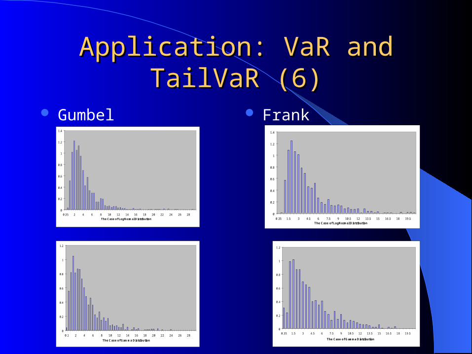
Application: VaR and TailVaR (6)Application: VaR and TailVaR (6)
Gumbel Frank
The Case of LogNormal Distribution
0
0.2
0.4
0.6
0.8
1
1.2
1.4
0.35 2 4 6 8 10 12 14 16 18 20 22 24 26 28
The Case of Gamma Distribution
0
0.2
0.4
0.6
0.8
1
1.2
0.1 2 4 6 8 10 12 14 16 18 20 22 24 26 28
The Case of LogNormal Distribution
0
0.2
0.4
0.6
0.8
1
1.2
1.4
0.35 1.5 3 4.5 6 7.5 9 10.5 12 13.5 15 16.5 18 19.5
The Case of Gamma Distribution
0
0.2
0.4
0.6
0.8
1
1.2
0.35 1.5 3 4.5 6 7.5 9 10.5 12 13.5 15 16.5 18 19.5
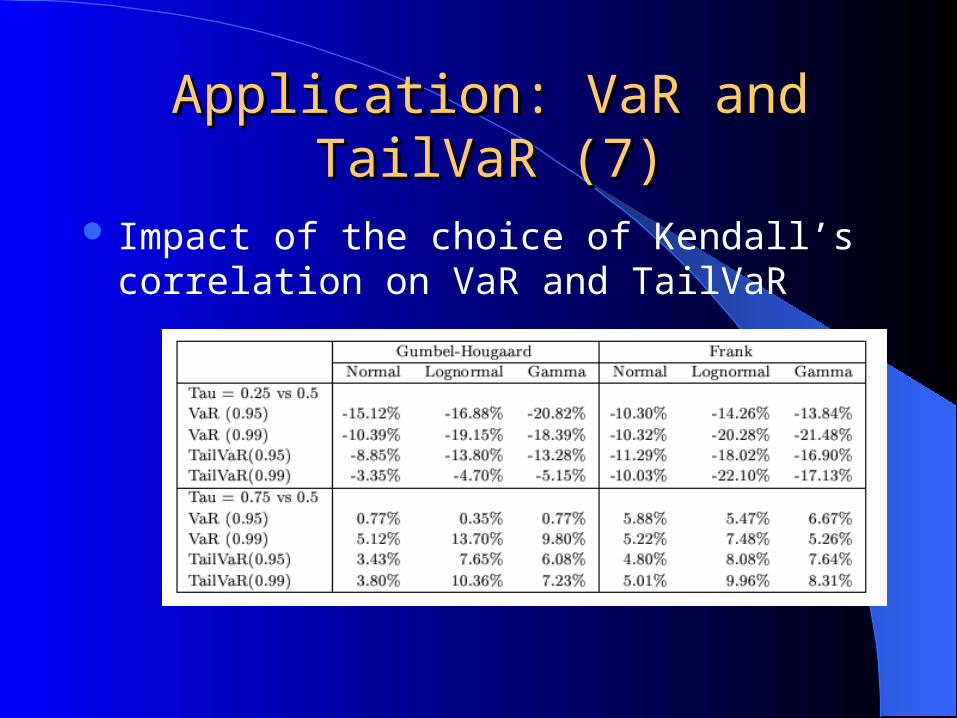
Application: VaR and TailVaR (7)Application: VaR and TailVaR (7)
Impact of the choice of Kendall’s correlation on VaR and TailVaR

ConclusionConclusion
Derived an algorithm for simulating multidimensional Archimedean copula.
Applied the algorithm to assess risk measures for marginals and copulas often used in insurance risk models.
Copula and marginals have a significant effect on economic capital