nested archimedean copulas meet r: the nacopula … nested archimedean copulas meet r: the nacopula...

JSS Journal of Statistical SoftwareMarch 2011, Volume 39, Issue 9. http://www.jstatsoft.org/

Nested Archimedean Copulas Meet R: The

nacopula Package

Marius HofertETH Zurich

Martin MachlerETH Zurich

Abstract

The package nacopula provides procedures for constructing nested Archimedean cop-ulas in any dimensions and with any kind of nesting structure, generating vectors ofrandom variates from the constructed objects, computing function values and probabili-ties of falling into hypercubes, as well as evaluation of characteristics such as Kendall’s tauand the tail-dependence coefficients. As by-products, algorithms for various distributions,including exponentially tilted stable and Sibuya distributions, are implemented. Detailedexamples are given.

Keywords: Archimedean copulas, nested Archimedean copulas, sampling algorithms, Kendall’stau, tail-dependence coefficients, exponentially tilted stable distribution, R.

1. Introduction

A copula is a multivariate distribution function with standard uniform univariate margins.Standard references for an introduction are Joe (1997) or Nelsen (2007).

Sklar (1959) shows that for any multivariate distribution function H with margins Fj , j ∈{1, . . . , d}, there exists a copula C such that

H(x1, . . . , xd) = C(F1(x1), . . . , Fd(xd)), x ∈ Rd. (1)

Conversely, given a copula C and arbitrary univariate distribution functions Fj , j ∈ {1, . . . , d},H defined by (1) is a distribution function with marginals Fj , j ∈ {1, . . . , d}. On one hand,Sklar’s Theorem tells us that we can decompose any given multivariate distribution functioninto its margins and a copula. By this decomposition, copulas allow us to study multivariatedistributions functions independently of the margins. This is of particular interest in statis-tics. On the other hand, Sklar’s Theorem provides a tool for constructing large classes ofmultivariate distributions and is therefore often used for sampling multivariate distributions

http://www.jstatsoft.org/

2 Nested Archimedean Copulas Meet R: The nacopula Package

via copulas. This is indispensable for many applications in the areas of statistics and finance.For sampling the multivariate distribution H it suffices to sample the common dependencestructure, given by the copula C, and to transform the obtained variates to the correct mar-gins Fj , j ∈ {1, . . . , d}. Since this transformation is usually easy to achieve (simply apply thegeneralized inverse F−j (y) = inf{x ∈ R : Fj(x) ≥ y} corresponding to Fj , j ∈ {1, . . . , d}, withthe convention that inf ∅ =∞), sampling from H usually boils down to sampling the copulaC under consideration.

Alongside elliptical copulas, i.e., the copulas arising from elliptical distributions via Sklar’sTheorem (see, e.g., Embrechts, Lindskog, and McNeil 2003), Archimedean copulas play animportant role in practical applications. In contrast to elliptical ones, Archimedean copulasare given explicitly in terms of a generator. They are able to capture different kinds of taildependencies, e.g., only upper tail dependence and no lower tail dependence or both lowerand upper tail dependence but of different magnitude. With the algorithm of Marshall andOlkin (1988), Archimedean copulas are usually easy to sample. Their functional symmetry(in uj , j = 1, . . . , d), also referred to as exchangeability, however, is often considered to bea drawback, e.g., in risk-management applications where the considered portfolios are typi-cally high-dimensional. To circumvent exchangeability, Archimedean copulas can be nestedwithin each other under certain conditions. The resulting copulas are referred to as “nestedArchimedean copulas” and allow to model hierarchical dependence structures.

The R package nacopula implements several functions for working with Archimedean andnested Archimedean copulas. In contrast to other R packages dealing with Archimedeancopulas, e.g., copula (Yan 2007; Kojadinovic and Yan 2010) or fCopulae (Wuertz et al. 2009),particular focus is put on nested Archimedean copulas. The R package nacopula is the firstR package dealing with these functions. It is available from the Comprehensive R ArchiveNetwork at http://CRAN.R-project.org/package=nacopula.

2. Archimedean copulas

2.1. Archimedean copulas and their properties

An Archimedean generator, or simply generator, is a continuous, decreasing function ψ :[0,∞] → [0, 1] which satisfies ψ(0) = 1, ψ(∞) := limt→∞ ψ(t) = 0, and which is strictlydecreasing on [0, inf{t : ψ(t) = 0}]. A d-dimensional copula is called Archimedean if it is ofthe form

C(u;ψ) = ψ(ψ−1(u1) + · · ·+ ψ−1(ud)), u ∈ [0, 1]d, (2)

for some generator ψ with inverse ψ−1 : [0, 1] → [0,∞], where ψ−1(0) = inf{t : ψ(t) = 0}.McNeil and Neslehova (2009) show that a generator defines a d-dimensional Archimedeancopula if and only if ψ is d-monotone, i.e., ψ is continuous on [0,∞], admits derivatives upto the order d − 2 satisfying (−1)k d

k

dtkψ(t) ≥ 0 for all k ∈ {0, . . . , d − 2}, t ∈ (0,∞), and

(−1)d−2 dd−2

dtd−2ψ(t) is decreasing and convex on (0,∞). A necessary and sufficient conditionfor an Archimedean generator ψ to generate a proper copula in all dimensions d is that ψis completely monotone, i.e., (−1)kψ(k)(t) ≥ 0 for all t ∈ (0,∞) and k ∈ N0, see Kimberling(1974) in the context of t-norms or Hofert (2010, p. 54) for a reworking in terms of copulas.Unless otherwise stated, we assume ψ to be completely monotone in what follows. Finally, let

http://CRAN.R-project.org/package=nacopula

Journal of Statistical Software 3

us note that the most simple dependence model, namely, independence, is provided by ψ(t) =exp(−t), with ψ−1(t) = log(t), and corresponding independence copula C(u) =

∏dj=1 uj .

The class of all completely monotone Archimedean generators is denoted by Ψ∞ in whatfollows. Bernstein’s Theorem, see, e.g., Feller (1971, p. 439), shows that this class coincideswith the class of Laplace-Stieltjes transforms of distribution functions F on the positive realline, where the Laplace-Stieltjes transform of F , also known as the Laplace transform of thedistribution, is defined as

LS[F ](t) :=

∫ ∞0

exp(−tx) dF (x), t ∈ [0,∞).

For a ψ ∈ Ψ∞, we hence have the relation

ψ = LS[F ], or, equivalently, F = LS−1[ψ].

for a distribution function F on the positive real line.

Note that the distribution function F is known for virtually all commonly used Archimedeangenerators, see, e.g., Hofert (2010, p. 62). The package nacopula currently provides the mostwidely used families of Ali-Mikhail-Haq, Clayton, Frank, Gumbel, and Joe; see Table 1 forthe generators and their corresponding distribution functions. Except for Clayton’s family,where we use a slightly simpler generator, these generators are the ones given in Nelsen (2007,pp. 116). Also note that for the families of Ali-Mikhail-Haq, Frank, and Joe, F is discretewith support N. In this case, ψ is of the form ψ(t) =

∑∞k=1 pk exp(−kt), t ∈ [0,∞], where

(pk)∞k=1 denotes the probability mass function corresponding to F .

These Archimedean copula families are provided as "acopula" R objects (for more informationabout the statistical software R, see R Development Core Team 2010), containing as slots thecorresponding generator ψ, psi, its inverse ψ−1, psiInv, and the “sampler”, i.e., randomnumber generator for V ∼ F , as V0:

R> library("nacopula")

R> ls("package:nacopula", pattern = "^cop[A-Z]")

[1] "copAMH" "copClayton" "copFrank" "copGumbel" "copJoe"

R> copClayton

Archimedean copula ("acopula"), family "Clayton"

It contains further slots, named

"psi", "psiInv", "paraConstr", "paraInterval", "V0", "tau",

"tauInv", "lambdaL", "lambdaLInv", "lambdaU", "lambdaUInv",

"nestConstr", "V01"

R> copClayton@psi

function (t, theta)

{

(1 + t)^(-1/theta)

}

<environment: namespace:nacopula>

R> copClayton@psiInv


Family Parameter ψ(t) V ∼ F = LS−1[ψ]

Ali-Mikhail-Haq θ ∈ [0, 1) (1− θ)/(exp(t)− θ) Geo(1− θ)Clayton θ ∈ (0,∞) (1 + t)−1/θ Γ(1/θ, 1)Frank θ ∈ (0,∞) − log(1− (1− e−θ) exp(−t))/θ Log(1− e−θ)Gumbel θ ∈ [1,∞) exp(−t1/θ) S(1/θ, 1, cosθ(π/(2θ)),1{θ=1}; 1)

Joe θ ∈ [1,∞) 1− (1− exp(−t))1/θ Sibuya(1/θ)

Table 1: Commonly used one-parameter Archimedean generators.

function (t, theta)

{

t^(-theta) - 1

}


R> copClayton@V0

function (n, theta)

{

rgamma(n, shape = 1/theta)

}


The majority of slots of such copula objects are functions, encoding properties of that copulafamily. In what follows, some of these functions are presented.

Sampling Archimedean copulas

From a mixture representation with respect to F , the following algorithm may be derived forsampling Archimedean copulas, see Marshall and Olkin (1988).

Algorithm 2.1

(1) sample V ∼ F = LS−1[ψ]

(2) sample Rj ∼ Exp(1), j ∈ {1, . . . , d}(3) set Uj = ψ(Rj/V ), j ∈ {1, . . . , d}(4) return U = (U1, . . . , Ud)

>

In order for this algorithm to be easily applied, we need to know how to sample the distributionfunctions F = LS−1[ψ]. For the families of Ali-Mikhail-Haq, Clayton, Frank, Gumbel, andJoe, see Table 1.

For the family of Ali-Mikhail-Haq, Geo(p) denotes a geometric distribution with success prob-ability p ∈ (0, 1] and probability mass function pk = p(1 − p)k−1 at k ∈ N (which in Ris dgeom(k, p)). For Clayton’s family, Γ(α, β) denotes the gamma distribution with shapeα ∈ (0,∞), rate β ∈ (0,∞), and density f(x) = βαxα−1 exp(−βx)/Γ(α), x ∈ (0,∞) (providedin R by [dpqr]gamma(., shape = α, rate = β)). For the family of Frank, Log(p) denotesa logarithmic distribution with parameter p ∈ (0, 1) and mass function pk = pk/(−k log(1−p))at k ∈ N. For sampling this distribution, we provide rlog(., p), using the algorithm “LK”


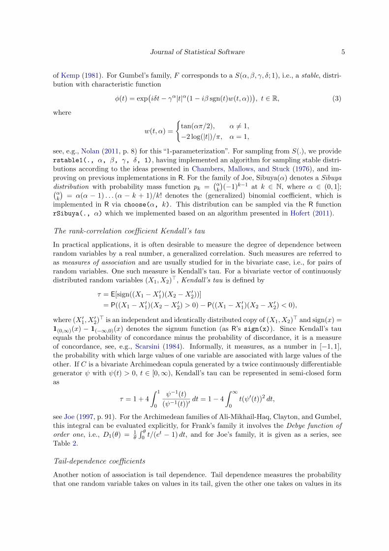
of Kemp (1981). For Gumbel’s family, F corresponds to a S(α, β, γ, δ; 1), i.e., a stable, distri-bution with characteristic function

φ(t) = exp(iδt− γα|t|α(1− iβ sgn(t)w(t, α))

), t ∈ R, (3)

where

w(t, α) =

{tan(απ/2), α 6= 1,

−2 log(|t|)/π, α = 1,

see, e.g., Nolan (2011, p. 8) for this “1-parameterization”. For sampling from S(.), we providerstable1(., α, β, γ, δ, 1), having implemented an algorithm for sampling stable distri-butions according to the ideas presented in Chambers, Mallows, and Stuck (1976), and im-proving on previous implementations in R. For the family of Joe, Sibuya(α) denotes a Sibuyadistribution with probability mass function pk =

(αk

)(−1)k−1 at k ∈ N, where α ∈ (0, 1];(

αk

)= α(α − 1) . . . (α − k + 1)/k! denotes the (generalized) binomial coefficient, which is

implemented in R via choose(α, k). This distribution can be sampled via the R functionrSibuya(., α) which we implemented based on an algorithm presented in Hofert (2011).

The rank-correlation coefficient Kendall’s tau

In practical applications, it is often desirable to measure the degree of dependence betweenrandom variables by a real number, a generalized correlation. Such measures are referred toas measures of association and are usually studied for in the bivariate case, i.e., for pairs ofrandom variables. One such measure is Kendall’s tau. For a bivariate vector of continuouslydistributed random variables (X1, X2)

>, Kendall’s tau is defined by

τ = E[sign((X1 −X ′1)(X2 −X ′2))]= P((X1 −X ′1)(X2 −X ′2) > 0)− P((X1 −X ′1)(X2 −X ′2) < 0),

where (X ′1, X′2)> is an independent and identically distributed copy of (X1, X2)

> and sign(x) =1(0,∞)(x) − 1(−∞,0)(x) denotes the signum function (as R’s sign(x)). Since Kendall’s tauequals the probability of concordance minus the probability of discordance, it is a measureof concordance, see, e.g., Scarsini (1984). Informally, it measures, as a number in [−1, 1],the probability with which large values of one variable are associated with large values of theother. If C is a bivariate Archimedean copula generated by a twice continuously differentiablegenerator ψ with ψ(t) > 0, t ∈ [0,∞), Kendall’s tau can be represented in semi-closed formas

τ = 1 + 4

∫ 1

0

ψ−1(t)

(ψ−1(t))′dt = 1− 4

∫ ∞0

t(ψ′(t))2 dt,

see Joe (1997, p. 91). For the Archimedean families of Ali-Mikhail-Haq, Clayton, and Gumbel,this integral can be evaluated explicitly, for Frank’s family it involves the Debye function oforder one, i.e., D1(θ) = 1

θ

∫ θ0 t/(e

t − 1) dt, and for Joe’s family, it is given as a series, seeTable 2.

Tail-dependence coefficients

Another notion of association is tail dependence. Tail dependence measures the probabilitythat one random variable takes on values in its tail, given the other one takes on values in its


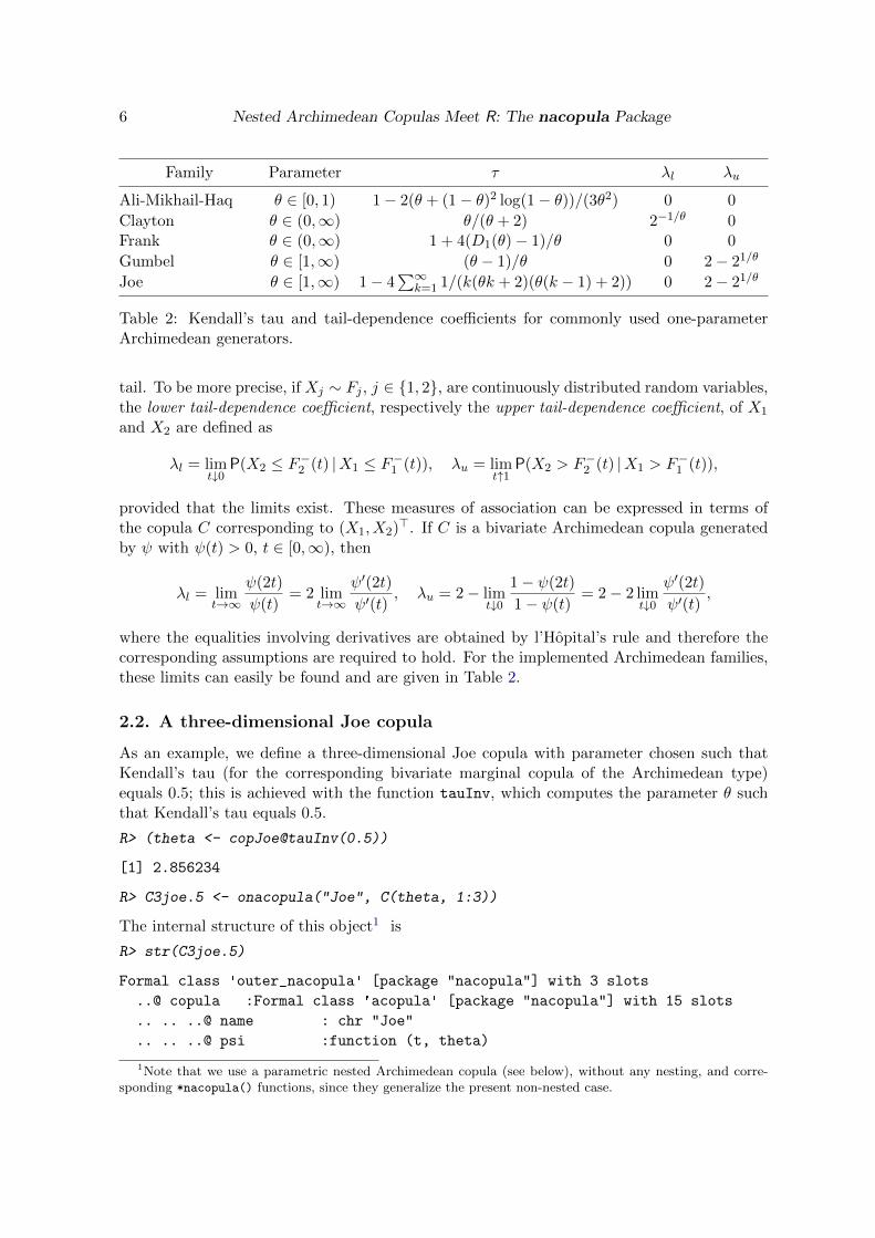
Family Parameter τ λl λu

Ali-Mikhail-Haq θ ∈ [0, 1) 1− 2(θ + (1− θ)2 log(1− θ))/(3θ2) 0 0

Clayton θ ∈ (0,∞) θ/(θ + 2) 2−1/θ 0Frank θ ∈ (0,∞) 1 + 4(D1(θ)− 1)/θ 0 0

Gumbel θ ∈ [1,∞) (θ − 1)/θ 0 2− 21/θ

Joe θ ∈ [1,∞) 1− 4∑∞

k=1 1/(k(θk + 2)(θ(k − 1) + 2)) 0 2− 21/θ

Table 2: Kendall’s tau and tail-dependence coefficients for commonly used one-parameterArchimedean generators.

tail. To be more precise, if Xj ∼ Fj , j ∈ {1, 2}, are continuously distributed random variables,the lower tail-dependence coefficient, respectively the upper tail-dependence coefficient, of X1

and X2 are defined as

λl = limt↓0

P(X2 ≤ F−2 (t) |X1 ≤ F−1 (t)), λu = limt↑1

P(X2 > F−2 (t) |X1 > F−1 (t)),

provided that the limits exist. These measures of association can be expressed in terms ofthe copula C corresponding to (X1, X2)

>. If C is a bivariate Archimedean copula generatedby ψ with ψ(t) > 0, t ∈ [0,∞), then

λl = limt→∞

ψ(2t)

ψ(t)= 2 lim

t→∞

ψ′(2t)

ψ′(t), λu = 2− lim

t↓0

1− ψ(2t)

1− ψ(t)= 2− 2 lim

t↓0

ψ′(2t)

ψ′(t),

where the equalities involving derivatives are obtained by l’Hopital’s rule and therefore thecorresponding assumptions are required to hold. For the implemented Archimedean families,these limits can easily be found and are given in Table 2.

2.2. A three-dimensional Joe copula

As an example, we define a three-dimensional Joe copula with parameter chosen such thatKendall’s tau (for the corresponding bivariate marginal copula of the Archimedean type)equals 0.5; this is achieved with the function tauInv, which computes the parameter θ suchthat Kendall’s tau equals 0.5.

R> (theta <- copJoe@tauInv(0.5))

[1] 2.856234

R> C3joe.5 <- onacopula("Joe", C(theta, 1:3))

The internal structure of this object1 is

R> str(C3joe.5)

Formal class 'outer_nacopula' [package "nacopula"] with 3 slots

..@ copula :Formal class 'acopula' [package "nacopula"] with 15 slots

.. .. ..@ name : chr "Joe"

.. .. ..@ psi :function (t, theta)

1Note that we use a parametric nested Archimedean copula (see below), without any nesting, and corre-sponding *nacopula() functions, since they generalize the present non-nested case.


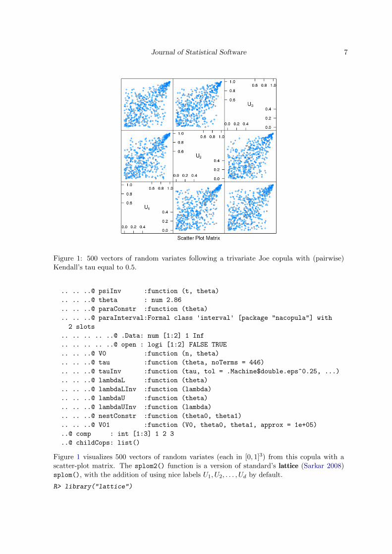
Figure 1: 500 vectors of random variates following a trivariate Joe copula with (pairwise)Kendall’s tau equal to 0.5.

.. .. ..@ psiInv :function (t, theta)

.. .. ..@ theta : num 2.86

.. .. ..@ paraConstr :function (theta)

.. .. ..@ paraInterval:Formal class 'interval' [package "nacopula"] with

2 slots

.. .. .. .. ..@ .Data: num [1:2] 1 Inf

.. .. .. .. ..@ open : logi [1:2] FALSE TRUE

.. .. ..@ V0 :function (n, theta)

.. .. ..@ tau :function (theta, noTerms = 446)

.. .. ..@ tauInv :function (tau, tol = .Machine$double.eps^0.25, ...)

.. .. ..@ lambdaL :function (theta)

.. .. ..@ lambdaLInv :function (lambda)

.. .. ..@ lambdaU :function (theta)

.. .. ..@ lambdaUInv :function (lambda)

.. .. ..@ nestConstr :function (theta0, theta1)

.. .. ..@ V01 :function (V0, theta0, theta1, approx = 1e+05)

..@ comp : int [1:3] 1 2 3

..@ childCops: list()

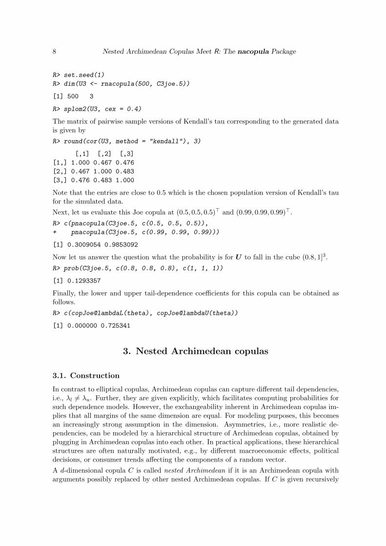
Figure 1 visualizes 500 vectors of random variates (each in [0, 1]3) from this copula with ascatter-plot matrix. The splom2() function is a version of standard’s lattice (Sarkar 2008)splom(), with the addition of using nice labels U1, U2, . . . , Ud by default.

R> library("lattice")


R> set.seed(1)

R> dim(U3 <- rnacopula(500, C3joe.5))

[1] 500 3

R> splom2(U3, cex = 0.4)

The matrix of pairwise sample versions of Kendall’s tau corresponding to the generated datais given by

R> round(cor(U3, method = "kendall"), 3)

[,1] [,2] [,3]

[1,] 1.000 0.467 0.476

[2,] 0.467 1.000 0.483

[3,] 0.476 0.483 1.000

Note that the entries are close to 0.5 which is the chosen population version of Kendall’s taufor the simulated data.

Next, let us evaluate this Joe copula at (0.5, 0.5, 0.5)> and (0.99, 0.99, 0.99)>.

R> c(pnacopula(C3joe.5, c(0.5, 0.5, 0.5)),

+ pnacopula(C3joe.5, c(0.99, 0.99, 0.99)))

[1] 0.3009054 0.9853092

Now let us answer the question what the probability is for U to fall in the cube (0.8, 1]3.

R> prob(C3joe.5, c(0.8, 0.8, 0.8), c(1, 1, 1))

[1] 0.1293357

Finally, the lower and upper tail-dependence coefficients for this copula can be obtained asfollows.

R> c(copJoe@lambdaL(theta), copJoe@lambdaU(theta))

[1] 0.000000 0.725341

3. Nested Archimedean copulas

3.1. Construction

In contrast to elliptical copulas, Archimedean copulas can capture different tail dependencies,i.e., λl 6= λu. Further, they are given explicitly, which facilitates computing probabilities forsuch dependence models. However, the exchangeability inherent in Archimedean copulas im-plies that all margins of the same dimension are equal. For modeling purposes, this becomesan increasingly strong assumption in the dimension. Asymmetries, i.e., more realistic de-pendencies, can be modeled by a hierarchical structure of Archimedean copulas, obtained byplugging in Archimedean copulas into each other. In practical applications, these hierarchicalstructures are often naturally motivated, e.g., by different macroeconomic effects, politicaldecisions, or consumer trends affecting the components of a random vector.

A d-dimensional copula C is called nested Archimedean if it is an Archimedean copula witharguments possibly replaced by other nested Archimedean copulas. If C is given recursively


C(· ;ψ0)

u1 C(· ;ψ1)

u2 u3

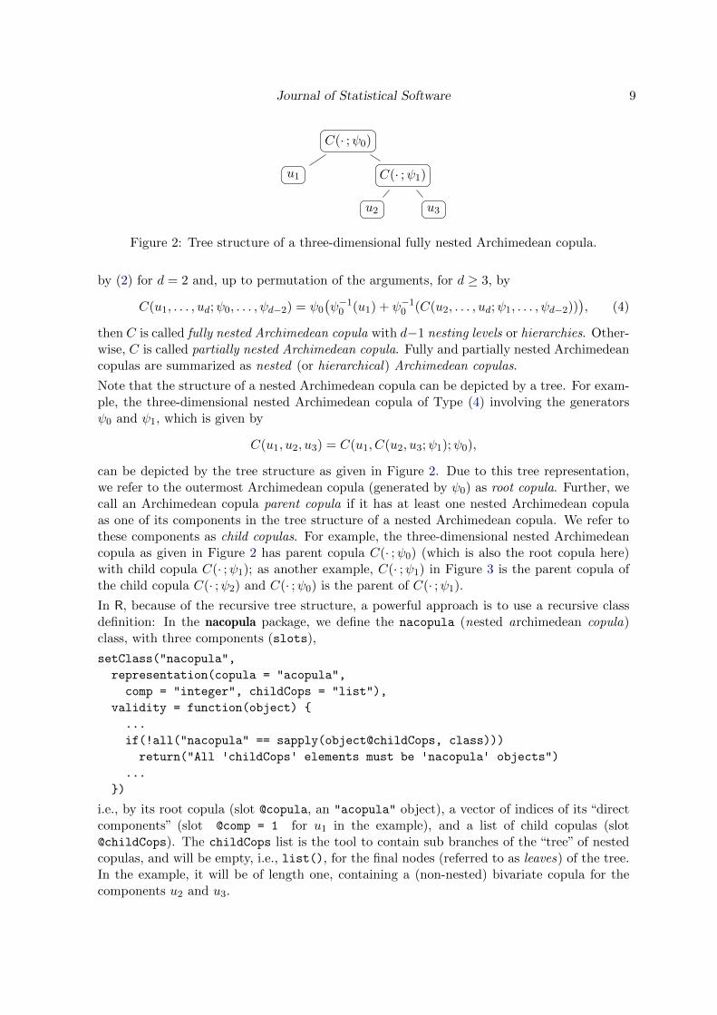
Figure 2: Tree structure of a three-dimensional fully nested Archimedean copula.

by (2) for d = 2 and, up to permutation of the arguments, for d ≥ 3, by

C(u1, . . . , ud;ψ0, . . . , ψd−2) = ψ0

(ψ−10 (u1) + ψ−10 (C(u2, . . . , ud;ψ1, . . . , ψd−2))

), (4)

then C is called fully nested Archimedean copula with d−1 nesting levels or hierarchies. Other-wise, C is called partially nested Archimedean copula. Fully and partially nested Archimedeancopulas are summarized as nested (or hierarchical) Archimedean copulas.

Note that the structure of a nested Archimedean copula can be depicted by a tree. For exam-ple, the three-dimensional nested Archimedean copula of Type (4) involving the generatorsψ0 and ψ1, which is given by

C(u1, u2, u3) = C(u1, C(u2, u3;ψ1);ψ0),

can be depicted by the tree structure as given in Figure 2. Due to this tree representation,we refer to the outermost Archimedean copula (generated by ψ0) as root copula. Further, wecall an Archimedean copula parent copula if it has at least one nested Archimedean copulaas one of its components in the tree structure of a nested Archimedean copula. We refer tothese components as child copulas. For example, the three-dimensional nested Archimedeancopula as given in Figure 2 has parent copula C(· ;ψ0) (which is also the root copula here)with child copula C(· ;ψ1); as another example, C(· ;ψ1) in Figure 3 is the parent copula ofthe child copula C(· ;ψ2) and C(· ;ψ0) is the parent of C(· ;ψ1).

In R, because of the recursive tree structure, a powerful approach is to use a recursive classdefinition: In the nacopula package, we define the nacopula (nested archimedean copula)class, with three components (slots),

setClass("nacopula",

representation(copula = "acopula",

comp = "integer", childCops = "list"),

validity = function(object) {

...

if(!all("nacopula" == sapply(object@childCops, class)))

return("All 'childCops' elements must be 'nacopula' objects")

...

})

i.e., by its root copula (slot @copula, an "acopula" object), a vector of indices of its “directcomponents” (slot @comp = 1 for u1 in the example), and a list of child copulas (slot@childCops). The childCops list is the tool to contain sub branches of the “tree” of nestedcopulas, and will be empty, i.e., list(), for the final nodes (referred to as leaves) of the tree.In the example, it will be of length one, containing a (non-nested) bivariate copula for thecomponents u2 and u3.


The class outer_nacopula is a version of the same class (i.e., it “contains” nacopula withoutany further slots), just with stricter validity checking, namely requiring that all componentsfrom all child copulas are exactly the set {1, 2, . . . , d}.setClass("outer_nacopula", contains = "nacopula",

validity = function(object) {

...

})

The onacopula() function2 allows to specify (outer) nacopulas with convenient specifica-tion of the nesting structure and parameters for each copula, using a “formula”-like nota-tion C(θ, c(i1, . . . , ic), list(C(..), . . . , C(..))) similar to the mathematical notation above; formore, see its help page. For example, (one parametrization of) the three-dimensional examplefrom Figure 2 is

R> (C3 <- onacopula("A", C(0.2, 1, C(0.8, 2:3))))

Nested Archimedean copula ("outer_nacopula"), with slot

'comp' = (1) and root

'copula' = Archimedean copula ("acopula"), family "AMH", theta= (0.2)

and 1 child copula

Nested Archimedean copula ("nacopula"), with slot

'comp' = (2, 3) and root

'copula' = Archimedean copula ("acopula"), family "AMH", theta= (0.8)

and *no* child copulas

This is a shortened form of the following.

R> stopifnot(identical(C3,

+ onacopula("A", C(0.2, 1, list(C(0.8, 2:3, list()))))))

The recursive definition (4) of nested Archimedean copulas not only leads to recursive classdefinitions in R, but also to recursive functions for computations involving such “nacopu-las”. All the following functions and methods (from our package nacopula) are definedrecursively, typically using lapply(x@childCops, <fun>): The utilities dim(), allComp(),printNacopula() (which is the hidden show() method), and the principal functionspnacopula() and rncopula() (via recursive utility rnchild()). As a simple example ofthese, pnacopula(x, u) simply evaluates the (recursive) Formula (4), recursively applyingitself to its child copulas:

pnacopula <- function(x, u) {

stopifnot(is.numeric(u), 0 <= u, u <= 1, length(u) >= dim(x))

C <- x@copula

th <- C@theta

C@psi(sum(unlist(lapply(u[x@comp], C@psiInv, theta = th)),

C@psiInv(unlist(lapply(x@childCops, pnacopula, u = u)), theta = th)),

theta = th)

}

In order for (4) to be indeed a proper copula, Joe (1997, p. 88) and McNeil (2008) present thesufficient nesting condition that ψ−1i ◦ ψj is completely monotone for all nodes (with parent

2In addition to onacopula(), there’s onacopulaL() (“L” for List) which requires a more formal specificationof the nesting structure by a list.


i and child j) appearing in a nested Archimedean copula. This condition can be derivedfrom a mixture representation of C based on the distribution functions F0 = LS−1[ψ0] andFij = LS−1[ψij(· ;V0)] where

ψij(t;x) = exp(−xψ−1i (ψj(t))

), t ∈ [0,∞], x ∈ (0,∞).

The sufficient nesting condition is often easily verified if all generators appearing in the nestedstructure come from the same parametric family. For each of the implemented Archimedeanfamilies of Ali-Mikhail-Haq, Clayton, Frank, Gumbel, and Joe, two generators ψi, ψj of thesame family with corresponding parameters θi, θj , respectively, fulfill the sufficient nestingcondition if θi ≤ θj ; equivalently, if τi ≤ τj for the corresponding Kendall’s tau. Verifyingthe sufficient nesting condition if ψi and ψj belong to different Archimedean families is usu-ally more complicated, see, Hofert (2010). Such combinations of Archimedean families aretherefore currently not implemented in the R package nacopula.

3.2. Sampling

If the sufficient nesting condition is fulfilled for all nodes in the nested Archimedean structure,the following algorithm, based on proposals by McNeil (2008) and Hofert (2011), may bederived for sampling nested Archimedean copulas.

Algorithm 3.1Let C be a nested Archimedean copula with root copula C0 generated by ψ0. Let U be avector of the same dimension as C.

(1) sample V0 ∼ F0 = LS−1[ψ0]

(2) for all components u of C0 that are nested Archimedean copulas do {(3) set C1 with generator ψ1 to the nested Archimedean copula u

(4) sample V01 ∼ F01 = LS−1[ψ01(· ;V0)](5) set C0 := C1, ψ0 := ψ1, and V0 := V01 and continue with (2)

(6) }(7) for all other components u of C0 do {(8) sample R ∼ Exp(1)

(9) set the component of U corresponding to u to ψ0(R/V0)

(10) }(11) return U

Note that for sampling nested Archimedean copulas when all generators involved belong tothe same parametric family, it suffices to know how to sample

V0 ∼ F0 = LS−1[ψ0], F01 = LS−1[ψ01(· ;V0)]

as all distribution functions Fij take the same form as F01, only the parameters may differ.In our R package nacopula, the supported Archimedean family objects therefore provide thethree slots V0, nestConstr, and V01, all functions. nestConstr, is a function(θ0, θ1) whichreturns TRUE if the sufficient nesting condition is fulfilled and V0 and V01 are random numbergenerating functions, generating V from Table 1 and V01 from Table 3, respectively. Forexample, for Ali-Mikhail-Haq,


Family Nesting V01 ∼ F01 = LS−1[ψ01(· ;V0)], α = θ0/θ1

Ali-Mikhail-Haq θ0 ≤ θ1 V0 + NB(V0, (1− θ1)/(1− θ0))Clayton θ0 ≤ θ1 S(α, 1, (cos(απ/2)V0)

1/α, V01{α=1},1{α 6=1}; 1)

Frank θ0 ≤ θ1∑V0

l=1 Vl, Vl ∼ pk = (θ1/(1− e−θ0))kpSibuya(α)k p

Log(1−e−θ1 )k

Gumbel θ0 ≤ θ1 S(α, 1, (cos(απ/2)V0)1/α, V01{α=1}; 1)

Joe θ0 ≤ θ1∑V0

l=1 Vl, Vl ∼ Sibuya(α)

Table 3: Sufficient nesting conditions and stochastic representations for V01.

R> copAMH@nestConstr

function (theta0, theta1)

{

copAMH@paraConstr(theta0) && copAMH@paraConstr(theta1) &&

theta1 >= theta0

}


R> copAMH@V01

function (V0, theta0, theta1)

{

rnbinom(length(V0), V0, (1 - theta1)/(1 - theta0)) + V0

}


Sampling strategies for F0 and F01 for many known Archimedean generators are presented inHofert (2008), Hofert (2010), and Hofert (2011). For the families of Ali-Mikhail-Haq, Clayton,Frank, Gumbel, and Joe, Table 3 summarizes stochastic representations for V0 and V01.

First note that for nested Archimedean copulas based on generators belonging to the sameArchimedean family, all implemented families indeed lead to proper copulas if the generatorson a more nested (inner) level have larger parameter values than the ones on a lower (outer)level. This is equivalent to saying that Kendall’s tau for a pair of random variables havinga bivariate Archimedean copula which resides on a deeper nesting level as margin has to belarger than or equal to the one for a pair of random variables having an Archimedean marginalcopula residing on a lower nesting level. Slightly more informally, the inner (or lower) nestedcomponents uj are more correlated than the outer (“higher up”) ones.

Some comments on the distributions F01 of V01 for the different implemented families: For thefamily of Ali-Mikhail-Haq, V01 admits the stochastic representation V0 +X, where X followsa negative binomial distribution with parameters as given in Table 3. The parameterizationis NB(r, p), r ∈ (0,∞), p ∈ (0, 1), with mass function pk =

(k+r−1r−1

)pr(1− p)k, k ∈ N0, which

in R is dnbinom(k, size=r, prob=p).

For Clayton’s family, F01 can be interpreted as a special case (take h = 1, α = θ0/θ1) of theexponentially tilted stable distribution

S(α, 1, (cos(απ/2)V0)1/α, V01{α=1}, h1{α6=1}; 1) (5)


with α ∈ (0, 1], h ∈ [0,∞), V0 ∈ (0,∞), and corresponding Laplace-Stieltjes transform

ψ(t) = exp(−V0((h+ t)α − hα)

), t ∈ [0,∞].

Hofert (2011) suggested a fast rejection algorithm for sampling this distribution. Devroye(2009) suggested an algorithm for sampling the exponentially tilted stable distribution

S(α, 1, cos(απ/2)1/α,1{α=1}, λ1{α 6=1}; 1)

with α ∈ (0, 1], λ ∈ [0,∞), and corresponding Laplace-Stieltjes transform

ψ(t) = exp(−((λ+ t)α − λα)

), t ∈ [0,∞].

One can easily check that by setting λ = hV1/α0 and generating Vλ with the algorithm of

Devroye (2009), the random variable V01 from F01 as given by (5) can be obtained via V01 =

V1/α0 Vλ. Therefore, the distribution as given in (5) may be sampled by either the algorithm

of Devroye (2009) or the one of Hofert (2011). The former author reports that the complexityof his algorithm is bounded, the latter author shows that the complexity of his algorithm isO(V0h

α). We implemented both algorithms for sampling (5) in the package nacopula anddecide for each drawn V0 which method is to be applied. As a simple rule, investigated byseveral parameter combinations, the default chooses the method of Hofert (2011) if V0h

α < 4and the one of Devroye (2009) otherwise. As mentioned before, note that for sampling nestedClayton copulas, we have h = 1. Further, E[V0] = 1/θ0. Hence, in the mean, the algorithm ofHofert (2011) is more often applied if θ0 > 1/4, equivalently, if Kendall’s tau for the bivariateArchimedean copula generated by ψ0 is greater than 1/9.

For the family of Gumbel, ψ01(t;V0) = exp(−V0tα), α = θ0/θ1, hence, see Table 1, F01

corresponds to the stable distribution as given in Table 3. For Joe’s family, V01 can be repre-sented as a V0-fold sum of independent and identically Sibuya distributed random variablesVk, k ∈ {1, . . . , V0}, which can be sampled with the R function rSibuya(., α) we provide.For large V0 an approximation based on a stable distribution may be used, see Hofert (2011).Finally, Frank’s family is more complicated. We refer to the source code of the packagenacopula and references therein for more details.

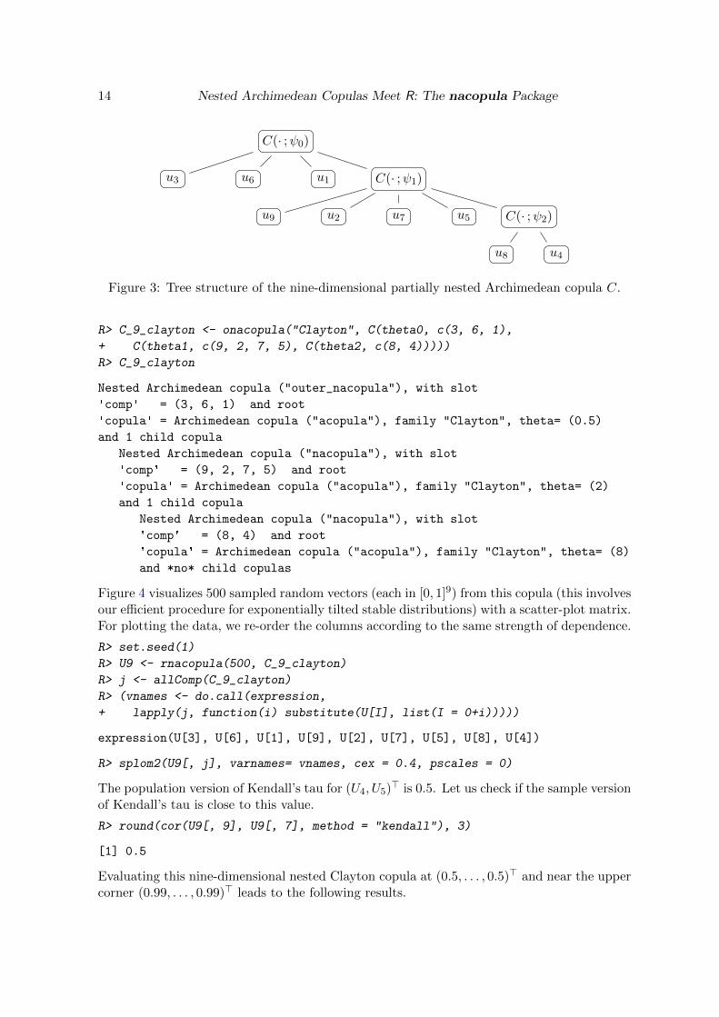
3.3. A nine-dimensional nested Clayton copula

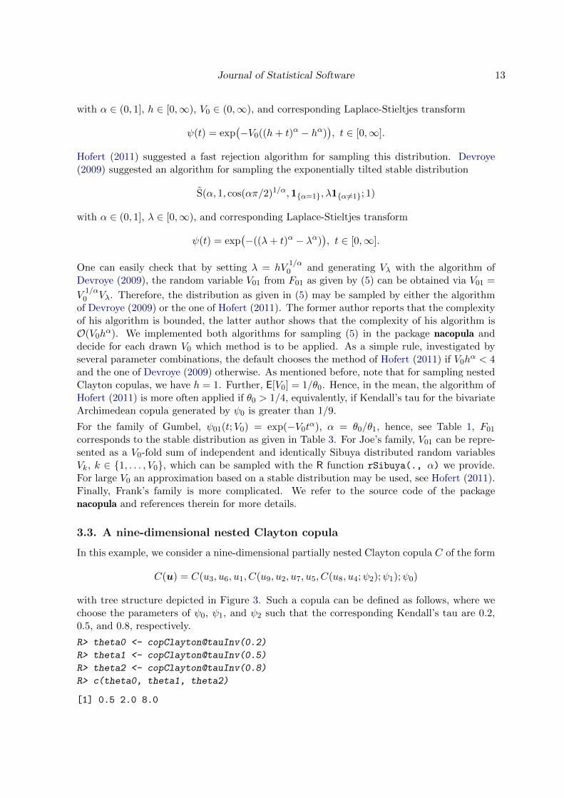
In this example, we consider a nine-dimensional partially nested Clayton copula C of the form

C(u) = C(u3, u6, u1, C(u9, u2, u7, u5, C(u8, u4;ψ2);ψ1);ψ0)

with tree structure depicted in Figure 3. Such a copula can be defined as follows, where wechoose the parameters of ψ0, ψ1, and ψ2 such that the corresponding Kendall’s tau are 0.2,0.5, and 0.8, respectively.

R> theta0 <- copClayton@tauInv(0.2)



R> c(theta0, theta1, theta2)

[1] 0.5 2.0 8.0


C(· ;ψ0)

u3 u6 u1 C(· ;ψ1)

u9 u2 u7 u5 C(· ;ψ2)

u8 u4

Figure 3: Tree structure of the nine-dimensional partially nested Archimedean copula C.

R> C_9_clayton <- onacopula("Clayton", C(theta0, c(3, 6, 1),

+ C(theta1, c(9, 2, 7, 5), C(theta2, c(8, 4)))))

R> C_9_clayton

Nested Archimedean copula ("outer_nacopula"), with slot

'comp' = (3, 6, 1) and root

'copula' = Archimedean copula ("acopula"), family "Clayton", theta= (0.5)

and 1 child copula


'comp' = (9, 2, 7, 5) and root

'copula' = Archimedean copula ("acopula"), family "Clayton", theta= (2)

and 1 child copula


'comp' = (8, 4) and root

'copula' = Archimedean copula ("acopula"), family "Clayton", theta= (8)

and *no* child copulas

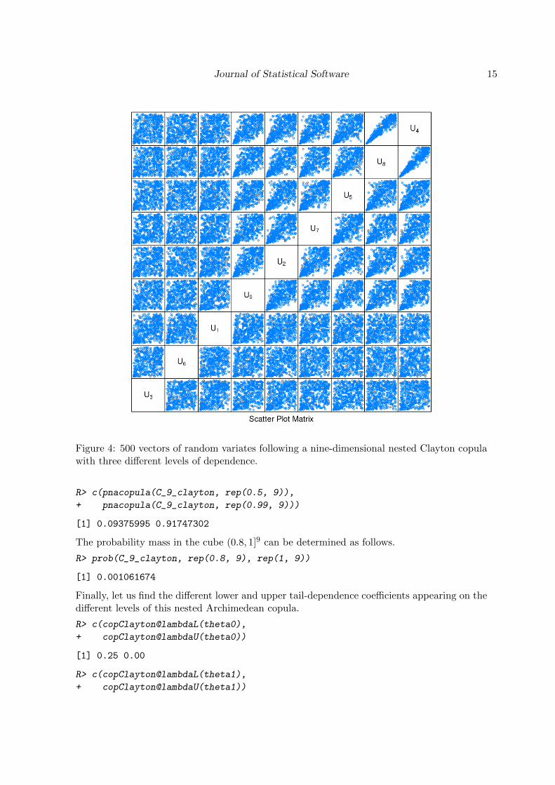
Figure 4 visualizes 500 sampled random vectors (each in [0, 1]9) from this copula (this involvesour efficient procedure for exponentially tilted stable distributions) with a scatter-plot matrix.For plotting the data, we re-order the columns according to the same strength of dependence.

R> set.seed(1)

R> U9 <- rnacopula(500, C_9_clayton)

R> j <- allComp(C_9_clayton)

R> (vnames <- do.call(expression,

+ lapply(j, function(i) substitute(U[I], list(I = 0+i)))))

expression(U[3], U[6], U[1], U[9], U[2], U[7], U[5], U[8], U[4])

R> splom2(U9[, j], varnames= vnames, cex = 0.4, pscales = 0)

The population version of Kendall’s tau for (U4, U5)> is 0.5. Let us check if the sample version

of Kendall’s tau is close to this value.

R> round(cor(U9[, 9], U9[, 7], method = "kendall"), 3)

[1] 0.5

Evaluating this nine-dimensional nested Clayton copula at (0.5, . . . , 0.5)> and near the uppercorner (0.99, . . . , 0.99)> leads to the following results.


Figure 4: 500 vectors of random variates following a nine-dimensional nested Clayton copulawith three different levels of dependence.

R> c(pnacopula(C_9_clayton, rep(0.5, 9)),

+ pnacopula(C_9_clayton, rep(0.99, 9)))

[1] 0.09375995 0.91747302

The probability mass in the cube (0.8, 1]9 can be determined as follows.

R> prob(C_9_clayton, rep(0.8, 9), rep(1, 9))

[1] 0.001061674

Finally, let us find the different lower and upper tail-dependence coefficients appearing on thedifferent levels of this nested Archimedean copula.

R> c(copClayton@lambdaL(theta0),

+ copClayton@lambdaU(theta0))

[1] 0.25 0.00




[1] 0.7071068 0.0000000



[1] 0.917004 0.000000

4. Outer power Archimedean copulas

For an Archimedean generator ψ ∈ Ψ∞, ψ(t1/θ) is also a valid generator in Ψ∞ for allθ ∈ [1,∞), see, e.g., Feller (1971, p. 441). The resulting copulas are referred to as outerpower Archimedean copulas. Note that two parametric Archimedean generators ψ(t1/θ0),θ0 ∈ [1,∞), and ψ(t1/θ1), θ1 ∈ [1,∞), of this type, constructed with the same“base”generatorψ(t), t ∈ [0,∞), fulfill the sufficient nesting condition if θ0 ≤ θ1. Therefore, one can build so-called nested outer power Archimedean copulas. Hofert (2011) derives some results for thesecopulas, including instructions for sampling the corresponding random variables V0 and V01,as well as an explicit formula for Kendall’s tau in terms of the Kendall’s tau of the copulagenerated by the base generator ψ. Further, note that if the tail-dependence coefficients exist,they are greater than or equal to the ones corresponding to the copula generated by the basegenerator. For the Archimedean families implemented in the package nacopula, these can allbe computed explicitly.

The goal of this section is to show how one might work with outer power Archimedeancopulas with the package nacopula. For now, we use the outer power transformation opower()

which generates an outer power family based on the provided copula family copbase withcorresponding parameter thetabase.

R> str(opower)

function (copbase, thetabase)

We believe that it is both more natural and flexible to work with copula families that aregeneralizations of our current families, each including the power as an extra parameter (suchthat theta, i.e., θ, will become 2-dimensional), rather than using the opower() constructionbelow. This section therefore should be considered mainly as an outlook to further featuresof the package nacopula, where this transformation is not required anymore for working withouter power Archimedean copulas.

Using this transformation, we define a valid outer power Clayton copula with base generatorof Clayton’s type and with base parameter such that Kendall’s tau equals 0.5.

R> thetabase <- copClayton@tauInv(0.5)

R> (opow.Clayton <- opower(copClayton, thetabase))

Archimedean copula ("acopula"), family "opower:Clayton"

It contains further slots, named

"psi", "psiInv", "paraConstr", "paraInterval", "V0", "tau",

"tauInv", "lambdaL", "lambdaLInv", "lambdaU", "lambdaUInv",

"nestConstr", "V01"

Based on this copula generator, we would like to define and sample a three-dimensional fullynested outer power Clayton copula with parameters such that Kendall’s tau are 2/3 and 0.75.


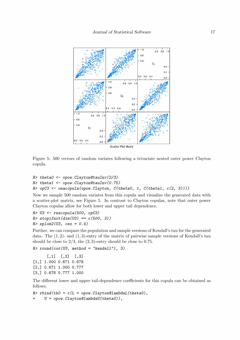
Figure 5: 500 vectors of random variates following a trivariate nested outer power Claytoncopula.

R> theta0 <- opow.Clayton@tauInv(2/3)

R> theta1 <- opow.Clayton@tauInv(0.75)

R> opC3 <- onacopula(opow.Clayton, C(theta0, 1, C(theta1, c(2, 3))))

Now we sample 500 random variates from this copula and visualize the generated data witha scatter-plot matrix, see Figure 5. In contrast to Clayton copulas, note that outer powerClayton copulas allow for both lower and upper tail dependence.

R> U3 <- rnacopula(500, opC3)

R> stopifnot(dim(U3) == c(500, 3))

R> splom2(U3, cex = 0.4)

Further, we can compare the population and sample versions of Kendall’s tau for the generateddata. The (1, 2)- and (1, 3)-entry of the matrix of pairwise sample versions of Kendall’s taushould be close to 2/3, the (2, 3)-entry should be close to 0.75.

R> round(cor(U3, method = "kendall"), 3)

[,1] [,2] [,3]

[1,] 1.000 0.671 0.678

[2,] 0.671 1.000 0.777

[3,] 0.678 0.777 1.000

The different lower and upper tail-dependence coefficients for this copula can be obtained asfollows.

R> rbind(th0 = c(L = opow.Clayton@lambdaL(theta0),

+ U = opow.Clayton@lambdaU(theta0)),


+ th1 = c(L = opow.Clayton@lambdaL(theta1),

+ U = opow.Clayton@lambdaU(theta1)))

L U

th0 0.7937005 0.4125989

th1 0.8408964 0.5857864

5. Session Information

R> toLatex(sessionInfo())

� R version 2.12.0 Patched (2010-11-28 r53696), x86_64-unknown-linux-gnu

� Locale: LC_CTYPE=de_CH.UTF-8, LC_NUMERIC=C, LC_TIME=en_US.UTF-8,LC_COLLATE=de_CH.UTF-8, LC_MONETARY=C, LC_MESSAGES=C, LC_PAPER=de_CH.UTF-8,LC_NAME=C, LC_ADDRESS=C, LC_TELEPHONE=C, LC_MEASUREMENT=de_CH.UTF-8,LC_IDENTIFICATION=C

� Base packages: base, datasets, graphics, grDevices, methods, stats, tools, utils

� Other packages: lattice 0.19-13, nacopula 0.4-3

� Loaded via a namespace (and not attached): grid 2.12.0, gsl 1.9-8

R> my.strsplit(packageDescription("nacopula")[["LastChanged"]])

$LastChangedRevision: 236 $

$LastChangedDate: 2010-08-18

14:00:06 +0200 (Wed, 18. Aug 2010) $

6. Conclusion

The package nacopula allows us to easily construct and work with nested Archimedean cop-ulas. First and foremost, fast sampling algorithms for these copulas are implemented. As aby-product, the package also provides related mathematical and random number generatingfunctions, e.g., efficient sampling algorithms for exponentially tilted stable and Sibuya dis-tributions. Further features include the evaluation of nested Archimedean copulas, as wellas computing probabilities of a random vector falling into a given hypercube. Concerningmeasures of association, Kendall’s tau and the tail-dependence coefficients are implemented.Currently supported Archimedean families include the well-known families of Ali-Mikhail-Haq, Clayton, Frank, Gumbel, and Joe. Each can be used in generalized form via “outerpower” transformations.

Acknowledgments

The first author (Willis Research Fellow) thanks Willis Re for financial support while thiswork was being completed.


References

Chambers JM, Mallows CL, Stuck BW (1976). “A Method for Simulating Stable RandomVariables.” Journal of the American Statistical Association, 71(354), 340–344.

Devroye L (2009). “Random Variate Generation for Exponentially and Polynomially TiltedStable Distributions.” ACM Transactions on Modeling and Computer Simulation, 19(4),18.

Embrechts P, Lindskog F, McNeil AJ (2003). “Modelling Dependence with Copulas and Ap-plications to Risk Management.” In S Rachev (ed.), Handbook of Heavy Tailed Distributionsin Finance, pp. 329–384.

Feller W (1971). An Introduction to Probability Theory and Its Applications, volume 2. 2ndedition. John Wiley & Sons.

Hofert M (2008). “Sampling Archimedean Copulas.” Computational Statistics & Data Anal-ysis, 52, 5163–5174.

Hofert M (2010). Sampling Nested Archimedean Copulas with Applications to CDO Pricing.Sudwestdeutscher Verlag fur Hochschulschriften AG & Co. KG. ISBN 978-3-8381-1656-3.PhD thesis.

Hofert M (2011). “Efficiently Sampling Nested Archimedean Copulas.” Computational Statis-tics & Data Analysis, 55, 57–70.

Joe H (1997). Multivariate Models and Dependence Concepts. Chapman & Hall/CRC.

Kemp AW (1981). “Efficient Generation of Logarithmically Distributed Pseudo-Random Vari-ables.” Journal of the Royal Statistical Society C, 30(3), 249–253.

Kimberling CH (1974). “A Probabilistic Interpretation of Complete Monotonicity.” Aequa-tiones Mathematicae, 10, 152–164.

Kojadinovic I, Yan J (2010). “Modeling Multivariate Distributions with Continuous MarginsUsing the copula R Package.” Journal of Statistical Software, 34(9), 1–20. URL http:

//www.jstatsoft.org/v34/i09/.

Marshall AW, Olkin I (1988). “Families of Multivariate Distributions.” Journal of the Amer-ican Statistical Association, 83, 834–841.

McNeil AJ (2008). “Sampling Nested Archimedean Copulas.” Journal of Statistical Compu-tation and Simulation, 78, 567–581.

McNeil AJ, Neslehova J (2009). “Multivariate Archimedean Copulas, d-monotone Functionsand l1-norm Symmetric Distributions.” The Annals of Statistics, 37(5b), 3059–3097.

Nelsen RB (2007). An Introduction to Copulas. Springer-Verlag, New York.

Nolan JP (2011). Stable Distributions – Models for Heavy Tailed Data. Birkhauser. Chapter 1online at http://academic2.american.edu/~jpnolan/stable/chap1.pdf.

http://www.jstatsoft.org/v34/i09/


http://academic2.american.edu/~jpnolan/stable/chap1.pdf


R Development Core Team (2010). R: A Language and Environment for Statistical Computing.R Foundation for Statistical Computing, Vienna, Austria. ISBN 3-900051-07-0, URL http:

//www.R-project.org/.

Sarkar D (2008). lattice: Multivariate Data Visualization with R. Springer-Verlag, New York.

Scarsini M (1984). “On Measures of Concordance.” Stochastica, 8(3), 201–218.

Sklar A (1959). “Fonctions de Repartition a n Dimensions et Leurs Marges.” Publications deL’Institut de Statistique de L’Universite de Paris, 8, 229–231.

Wuertz D, et al. (2009). fCopulae: Dependence Structures with Copulas. R package ver-sion 2110.78, URL http://CRAN.R-project.org/package=fCopulae.

Yan J (2007). “Enjoy the Joy of Copulas: With a Package copula.” Journal of StatisticalSoftware, 21(4), 1–21. URL http://www.jstatsoft.org/v21/i04/.

Affiliation:

Marius HofertDepartment of MathematicsETH Zurich8092 Zurich, SwitzerlandE-mail: [email protected]: http://www.math.ethz.ch/~hofertj/

Martin MachlerSeminar fur Statistik, HG G 16ETH Zurich8092 Zurich, SwitzerlandE-mail: [email protected]: http://stat.ethz.ch/people/maechler/

Journal of Statistical Software http://www.jstatsoft.org/

published by the American Statistical Association http://www.amstat.org/

Volume 39, Issue 9 Submitted: 2010-07-01March 2011 Accepted: 2010-11-15

http://www.R-project.org/

http://www.R-project.org/

http://CRAN.R-project.org/package=fCopulae


mailto:[email protected]

http://www.math.ethz.ch/~hofertj/

mailto:[email protected]

http://stat.ethz.ch/people/maechler/

http://www.jstatsoft.org/

http://www.amstat.org/

nested archimedean copulas meet r: the nacopula … nested archimedean copulas meet r: the nacopula...

Documents