multivariate copula models at work - welcome to rmetrics · multivariate extension of sklar’s...
TRANSCRIPT
Multivariate copula models at work
Matthias Fischer
University of Erlangen-Nuremberg, GermanyHomepage: www.statistik.wiso.uni-erlangen.deE-mail: [email protected]
Meilisalp 2009R-Metrics Workshop
Fischer () Meilisalp 2009 1 / 52
Outline
1 Introduction to copulas
2 Construction of d-copulas
3 Empirical results
Fischer () Meilisalp 2009 2 / 52
Introduction to copulas
1. Introduction to copulas
Fischer () Meilisalp 2009 3 / 52
Introduction to copulas
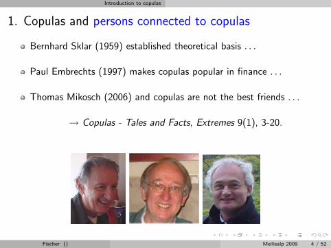
1. Copulas and persons connected to copulas
Bernhard Sklar (1959) established theoretical basis . . .
Paul Embrechts (1997) makes copulas popular in finance . . .
Thomas Mikosch (2006) and copulas are not the best friends . . .
→ Copulas - Tales and Facts, Extremes 9(1), 3-20.
Fischer () Meilisalp 2009 4 / 52
Introduction to copulas
1. The ”copula craze”
”When I started writing the paper (Mikosch, 2005) in 2003 a Googlesearch of the word copula gave 10,000 responses. In september 2005 thesame search gives 650,000 responses. There is an explosion of activity.
WHAT IS GOING ON?”
Personal update in November, 2007: 1,400,000 responses.
Update in June, 2009 (Meilisalp): ?????.
Fischer () Meilisalp 2009 5 / 52
Introduction to copulas
1. Defining bivariate copulas
Ironical: Copulas are ”Thomas Mikosch’s best friends”
Formal: Copulas are distribution functions on the unit-cube withuniform marginals. For d = 2,
1 Boundary conditions:C(u, 0) = C(0, v) = 0 and C(u, 1) = C(1, u) = u.
2 Two-increasing condition: For u1 ≤ u2 and v1 ≤ v2 holdsC(u2, v2)− C(u2, v1)− C(u1, v2) + C(u1, v1) ≥ 0.
Informal: Copulas incorporate the information on the dependencestructure between two or more random variables.
Fischer () Meilisalp 2009 6 / 52
Introduction to copulas
1. The fundamental theorem on copulas
Theorem (Sklar, 1959)
Let FX,Y denote a joint distribution function with margins FX and FY .Then there exists a copula C such that
FX,Y (x, y) = C(FX(x), FY (y)).
If FX and FY are continuous, then C is unique.
Example
If the random variables X and Y are independent,
FX,Y (x, y) = FX(x) · FY (y) = C(FX(x), FY (y)) with C(u, v) = u · v.
Independence copula: Π(u, v) ≡ C(u, v) = u · v,
Fischer () Meilisalp 2009 7 / 52
Introduction to copulas
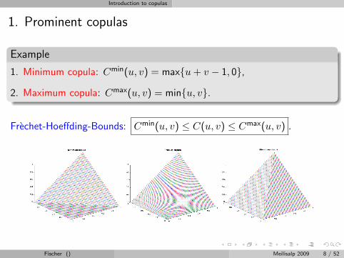
1. Prominent copulas
Example
1. Minimum copula: Cmin(u, v) = max{u + v − 1, 0},
2. Maximum copula: Cmax(u, v) = min{u, v}.
Frechet-Hoeffding-Bounds: Cmin(u, v) ≤ C(u, v) ≤ Cmax(u, v) .
Fischer () Meilisalp 2009 8 / 52
Introduction to copulas
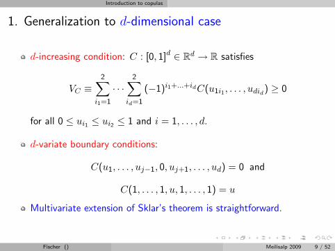
1. Generalization to d-dimensional case
d-increasing condition: C : [0, 1]d ∈ Rd → R satisfies
VC ≡2∑
i1=1
· · ·2∑
id=1
(−1)i1+...+idC(u1i1 , . . . , udid) ≥ 0
for all 0 ≤ ui1 ≤ ui2 ≤ 1 and i = 1, . . . , d.
d-variate boundary conditions:
C(u1, . . . , uj−1, 0, uj+1, . . . , ud) = 0 and
C(1, . . . , 1, u, 1, . . . , 1) = u
Multivariate extension of Sklar’s theorem is straightforward.
Fischer () Meilisalp 2009 9 / 52
Construction of d-copulas
2. Construction of d-copulas
Fischer () Meilisalp 2009 10 / 52

Construction of d-copulas
2. Observations and motivation
1 Most of the literature on copulas focusses on the bivariate case whichhas been extensively discussed in the past years.
2 In contrast, there were only a few construction schemes forhigher-dimensional copulas, namely Archimedean and ellipticalcopulas.
3 From 2005 on, a handful of extensions and innovations appeared, e.g.Morillas (2005), Palmitesta & Provasi (2005), Aas et al. (2006), Savu& Trede (2006), Liebscher (2008).
4 Newertheless, ”multivariate” often means setting ”d = 3” in theempirical part (if there was an application considered at all).
5 A comprehensive comparison between these approaches was missing.
Fischer () Meilisalp 2009 11 / 52
Construction of d-copulas
2. Result(s) and basis for this talk . . .
Matthias Fischer, Christian Kock, S. Schluter, F. Weigert (2009)An empirical analysis of multivariate copula models.Quantitative Finance (accepted for publication)
→ ”Comparison of the different approaches for d = 4”
Matthias Fischer and Christian Kock (2009)Constructing and generalizing given multivariate copulas.Statistics (accepted for publication)
→ ”A copula model including Liebscher & Morrillas approach”
Fischer () Meilisalp 2009 12 / 52
Construction of d-copulas
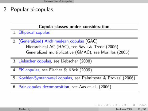
2. Popular d-copulas
Copula classes under consideration1. Elliptical copulas
2. (Generalized) Archimedean copulas (GAC)Hierarchical AC (HAC), see Savu & Trede (2006)Generalized multiplicative (GMAC), see Morillas (2005)
3. Liebscher copulas, see Liebscher (2008)
4. FK copulas, see Fischer & Kock (2009)
5. Koehler-Symanowski copulas, see Palmitesta & Provasi (2006)
6. Pair copulas decomposition, see Aas et al. (2006)
Fischer () Meilisalp 2009 13 / 52
Construction of d-copulas
2. Popular d-copulas - relevant literature
Liebscher, E. (2008).Construction of asymetric multivariate copulas.Journal of Multivariate Analysis, 99, 2234-2250.
Morillas, P. M. (2005).A method to obtain new copulas from a given one.Metrika 61, 169-184.
Palmitesta, P.; Provasi, C. (2005).Aggregation of Dependent Risks using the KS Copula Function.Computational Economics 25, 189-205.
Aas, K.; Czado, C.; Frigessi, A.; Bakken, H. (2006).Pair Copula Constructions of Multiple Dependence.Working Paper of the Norwegian Computing Center.
Savu, C.; Trede, M. (2006).Hierarchical Archimedean Copulas.Working Paper, University of Munster.
Fischer () Meilisalp 2009 14 / 52
Construction of d-copulas
2.1 Elliptical copulas
Recall Sklar’s theorem: You can extract the underlying (unique)copula from a multivariate distribution. For d = 2,
C(u, v) = F (F−1(u), F−1(v)).
Elliptical copulas are the copulas associated to elliptical distribution.
Popular elliptical copulas:1 Gaussian copula2 Student-t copula (”desert island copula”)3 Symmetric generalized hyperbolic copula.
Shortcomings: Assuming a certain kind of symmetry, no closed form.
Advantage: Applicable for high dimensions.
Fischer () Meilisalp 2009 15 / 52
Construction of d-copulas
2.2 Plain Archimedean copulas
A function ϕ : [0, 1] 7→ [0,∞), ϕ(1) = 0 is said to be completelymonotonic of order d, if (−1)iϕ(i)(x) ≥ 0. for all i ≤ d.
For a given generator function ϕ (assumed to be completelymonotonic of order d) define a d-copula (”Archimedean Copulas”) by
C(u1, . . . , ud) = ϕ−1 (ϕ(u1) + ϕ(u2) + · · ·+ ϕ(ud))
Example
Clayton copula with generator ϕ(t) = 1θ (t−θ − 1) for θ > 0.
C(u) =(u−θ
1 + · · ·+ u−θd − d + 1
)−1/θ, θ > 0.
AC in general: (−) not very flexible, (+) closed form solution, admitsdifferent kind of asymmetries.
Fischer () Meilisalp 2009 16 / 52
Construction of d-copulas
2.2 Generalized Archimedean copulas (Basic idea)
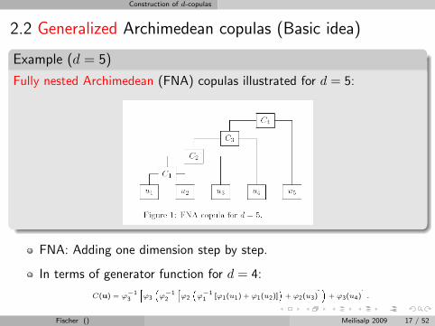
Example (d = 5)
Fully nested Archimedean (FNA) copulas illustrated for d = 5:
FNA: Adding one dimension step by step.
In terms of generator function for d = 4:
C(u) = ϕ−13
hϕ3
�ϕ−12
hϕ2
�ϕ−11 [ϕ1(u1) + ϕ1(u2)]
�+ ϕ2(u3)
i�+ ϕ3(u4)
i.
Fischer () Meilisalp 2009 17 / 52
Construction of d-copulas
2.2 Hierarchical Archimedean copulas (Basic idea)
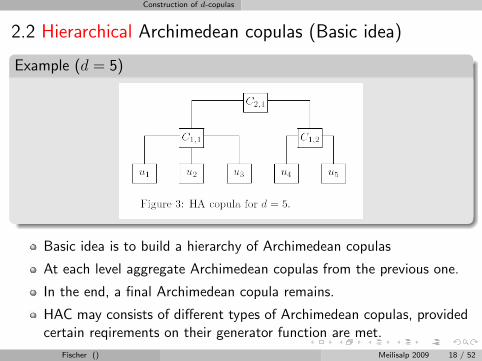
Example (d = 5)
Basic idea is to build a hierarchy of Archimedean copulas
At each level aggregate Archimedean copulas from the previous one.
In the end, a final Archimedean copula remains.
HAC may consists of different types of Archimedean copulas, providedcertain reqirements on their generator function are met.
Fischer () Meilisalp 2009 18 / 52
Construction of d-copulas
2.2 Hierarchical Archimedean copulas (Basic idea)
HAC were already discussed by Joe (1999) or Whelan (2004).
Savu & Trede (2006) derive the (general) HAC density and apply it tostock return data for d = 12.
Okhrin, Ohkrin & Schmid (2007) deal with finding the optimal HACstructure based parametric copula families, e.g. d = 3
C(φ, α; (123)) = C((φ, φ), (α, α); ((12)3))
= C((φ, φ), (α, α); ((1(23))
= C((φ, φ), (α, α); ((2(13))
McNeil (2006) deals with simulating from GAC’s.
Fischer () Meilisalp 2009 19 / 52
Construction of d-copulas
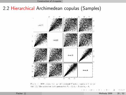
2.2 Hierarchical Archimedean copulas (Samples)
Fischer () Meilisalp 2009 20 / 52
Construction of d-copulas
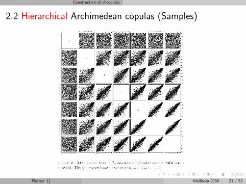
2.2 Hierarchical Archimedean copulas (Samples)
Fischer () Meilisalp 2009 21 / 52
Construction of d-copulas
2.2 Generalized multiplicative Archimedean copulas
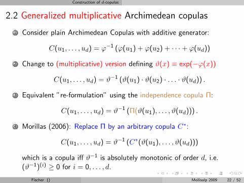
1 Consider plain Archimedean Copulas with additive generator:
C(u1, . . . , ud) = ϕ−1 (ϕ(u1) + ϕ(u2) + · · ·+ ϕ(ud))
2 Change to (multiplicative) version defining ϑ(x) ≡ exp(−ϕ(x))
C(u1, . . . , ud) = ϑ−1 (ϑ(u1) · ϑ(u2) · . . . · ϑ(ud)) .
3 Equivalent ”re-formulation” using the independence copula Π:
C(u1, . . . , ud) = ϑ−1 (Π(ϑ(u1), . . . , ϑ(ud))) .
4 Morillas (2006): Replace Π by an arbitrary copula C∗:
C(u1, . . . , ud) = ϑ−1 (C∗(ϑ(u1), . . . , ϑ(ud)))
which is a copula iff ϑ−1 is absolutely monotonic of order d, i.e.(ϑ−1)(i) ≥ 0 for i = 0, . . . , d.
Fischer () Meilisalp 2009 22 / 52
Construction of d-copulas
2.3 Liebscher copulas (Basic idea)
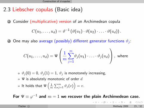
1 Consider (multiplicative) version of an Archimedean copula
C(u1, . . . , ud) = ϑ−1 (ϑ(u1) · ϑ(u2) · . . . · ϑ(ud)) .
2 One may also average (possibly) different generator functions ϑj :
C(u1, . . . , ud) = Ψ
1
m
m∑j=1
ϑj(u1) · . . . · ϑj(ud)
, where
ϑj(0) = 0, ϑj(1) = 1, ϑj is monotonely increasing,
Ψ is absolutely monotonic of order d
It holds that Ψ(
1m
∑mj=1 ϑj(v)
)= v.
For Ψ ≡ ϕ−1 and m = 1 we recover the plain Archimedean case.
Fischer () Meilisalp 2009 23 / 52
Construction of d-copulas
2.3 Liebscher copulas
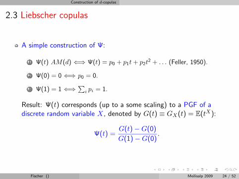
A simple construction of Ψ:
1 Ψ(t) AM(d) ⇐⇒ Ψ(t) = p0 + p1t + p2t2 + . . . (Feller, 1950).
2 Ψ(0) = 0 ⇐⇒ p0 = 0.
3 Ψ(1) = 1 ⇐⇒∑
i pi = 1.
Result: Ψ(t) corresponds (up to a some scaling) to a PGF of adiscrete random variable X, denoted by G(t) ≡ GX(t) = E(tX):
Ψ(t) =G(t)−G(0)
G(1)−G(0).
Fischer () Meilisalp 2009 24 / 52
Construction of d-copulas
2.3 Liebscher copulas
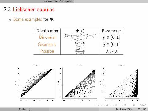
Some examples for Ψ:
Distribution Ψ(t) Parameter
Binomial ((1−p)+pt)n−(1−p)n
1−(1−p)n p ∈ (0, 1]
Geometric (1−q)t1−qt q ∈ (0, 1]
Poisson eλt−1eλ−1
λ > 0
Fischer () Meilisalp 2009 25 / 52
Construction of d-copulas
2.3 Liebscher copulas
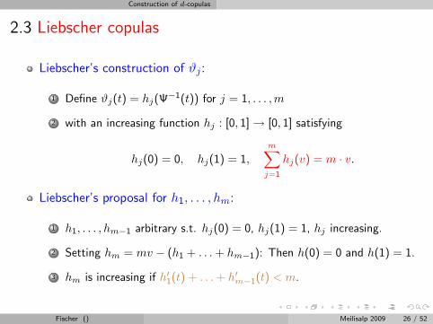
Liebscher’s construction of ϑj :
1 Define ϑj(t) = hj(Ψ−1(t)) for j = 1, . . . ,m
2 with an increasing function hj : [0, 1] → [0, 1] satisfying
hj(0) = 0, hj(1) = 1,m∑
j=1
hj(v) = m · v.
Liebscher’s proposal for h1, . . . , hm:
1 h1, . . . , hm−1 arbitrary s.t. hj(0) = 0, hj(1) = 1, hj increasing.
2 Setting hm = mv − (h1 + . . . + hm−1): Then h(0) = 0 and h(1) = 1.
3 hm is increasing if h′1(t) + . . . + h′m−1(t) < m.
Fischer () Meilisalp 2009 26 / 52
Construction of d-copulas
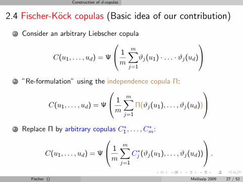
2.4 Fischer-Kock copulas (Basic idea of our contribution)
1 Consider an arbitrary Liebscher copula
C(u1, . . . , ud) = Ψ
1
m
m∑j=1
ϑj(u1) · . . . · ϑj(ud)
2 ”Re-formulation” using the independence copula Π:
C(u1, . . . , ud) = Ψ
1
m
m∑j=1
Π(ϑj(u1), . . . , ϑj(ud))
3 Replace Π by arbitrary copulas C∗
1 , . . . , C∗m:
C(u1, . . . , ud) = Ψ
1
m
m∑j=1
C∗j (ϑj(u1), . . . , ϑj(ud))
.
Fischer () Meilisalp 2009 27 / 52
Construction of d-copulas
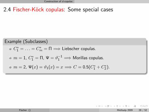
2.4 Fischer-Kock copulas: Some special cases
Example (Subclasses)
C∗1 = . . . = C∗
m = Π =⇒ Liebscher copulas.
m = 1, C∗1 = Π, Ψ = ϑ−1
1 =⇒ Morillas copulas.
m = 2, Ψ(x) = ϑ1(x) = x =⇒ C = 0.5(C∗1 + C∗
2 ).
Fischer () Meilisalp 2009 28 / 52
Construction of d-copulas
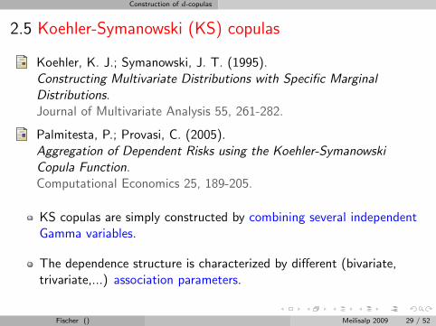
2.5 Koehler-Symanowski (KS) copulas
Koehler, K. J.; Symanowski, J. T. (1995).Constructing Multivariate Distributions with Specific MarginalDistributions.Journal of Multivariate Analysis 55, 261-282.
Palmitesta, P.; Provasi, C. (2005).Aggregation of Dependent Risks using the Koehler-SymanowskiCopula Function.Computational Economics 25, 189-205.
KS copulas are simply constructed by combining several independentGamma variables.
The dependence structure is characterized by different (bivariate,trivariate,...) association parameters.
Fischer () Meilisalp 2009 29 / 52
Construction of d-copulas
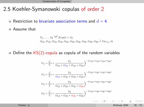
2.5 Koehler-Symanowski copulas of order 2
Restriction to bivariate association terms and d = 4.
Assume that
Y1, . . . , Y4iid∼ Exp(λ = 1),
G11, G12, G13, G14, G22, G23, G24, G33, G34, G44i∼ Γ(αij , 1)
Define the KS(2)-copula as copula of the random variables
U1 =
�1 +
Y1
G11 + G12 + G13 + G14
�−(α11+α12+α13+α14)
U2 =
�1 +
Y2
G12 + G22 + G23 + G24
�−(α12+α22+α23+α24)
U3 =
�1 +
Y3
G13 + G23 + G33 + G34
�−(α13+α23+α33+α34)
U4 =
�1 +
Y4
G14 + G24 + G34 + G44
�−(α14+α24+α34+α44)
Fischer () Meilisalp 2009 30 / 52
Construction of d-copulas
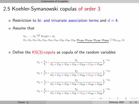
2.5 Koehler-Symanowski copulas of order 3
Restriction to bi- and trivariate association terms and d = 4.
Assume that
Y1, . . . , Y4iid∼ Exp(λ = 1),
G1, G2, G3, G4, G12, G13, G14, G23, G24, G34, G123, G134, G124, G234| {z }i∼ Γ(αijk, 1)
Define the KS(3)-copula as copula of the random variables
U1 =
�1 +
Y1
G1 + G12 + G13 + G14 + G123 + G124 + G134
�−α1.
U2 =
�1 +
Y2
G2 + G12 + G23 + G24 + G234 + G124 + G123
�−α2.
U3 =
�1 +
Y3
G3 + G13 + G23 + G34 + G123 + G134 + G234
�−α3.
U4 =
�1 +
Y4
G4 + G14 + G24 + G34 + G124 + G134 + G234
�−α4.
Fischer () Meilisalp 2009 31 / 52
Construction of d-copulas
2.5 Koehler-Symanowski (KS) copulas
Application of multivariate variable transformation reveals
1 the copula in closed form,
2 the copula density in closed form.
Several kinds of asymmetries and tail dependence behaviour can berebuild.
The Clayton copula is included as special case.
Whereas Palmitesta & Provasi (2005) only use the KS(2)-copula, wealso implemented the KS(3) and the KS(4)-copula!
Fischer () Meilisalp 2009 32 / 52
Construction of d-copulas
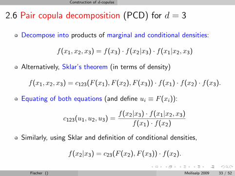
2.6 Pair copula decomposition (PCD) for d = 3
Decompose into products of marginal and conditional densities:
f(x1, x2, x3) = f(x3) · f(x2|x3) · f(x1|x2, x3)
Alternatively, Sklar’s theorem (in terms of density)
f(x1, x2, x3) = c123(F (x1), F (x2), F (x3)) · f(x1) · f(x2) · f(x3).
Equating of both equations (and define ui ≡ F (xi)):
c123(u1, u2, u3) =f(x2|x3) · f(x1|x2, x3)
f(x1) · f(x2)
Similarly, using Sklar and definition of conditional densities,
f(x2|x3) = c23(F (x2), F (x3)) · f(x2).
Fischer () Meilisalp 2009 33 / 52
Construction of d-copulas
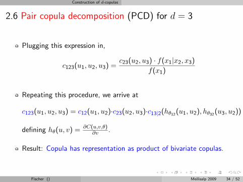
2.6 Pair copula decomposition (PCD) for d = 3
Plugging this expression in,
c123(u1, u2, u3) =c23(u2, u3) · f(x1|x2, x3)
f(x1)
Repeating this procedure, we arrive at
c123(u1, u2, u3) = c12(u1, u2)·c23(u2, u3)·c13|2(hθ12(u1, u2), hθ32(u3, u2))
defining hθ(u, v) = ∂C(u,v,θ)∂v .
Result: Copula has representation as product of bivariate copulas.
Fischer () Meilisalp 2009 34 / 52
Construction of d-copulas
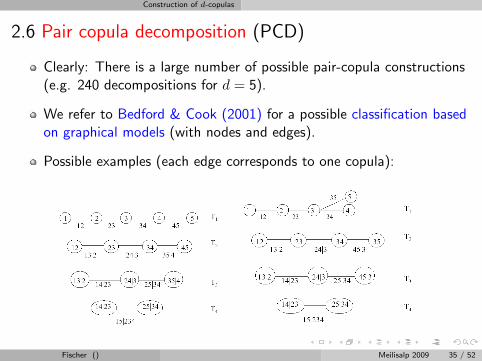
2.6 Pair copula decomposition (PCD)
Clearly: There is a large number of possible pair-copula constructions(e.g. 240 decompositions for d = 5).
We refer to Bedford & Cook (2001) for a possible classification basedon graphical models (with nodes and edges).
Possible examples (each edge corresponds to one copula):
Fischer () Meilisalp 2009 35 / 52

Empirical results
3. Comparison of d-copula models
Fischer () Meilisalp 2009 36 / 52
Empirical results
3. Basic setting of our study in short
1 Due to technical restrictions we focussed on d = 4.
2 In total we estimated about 30 different copula models (details on thenext slide) for each data set.
3 In our paper, results can be found for
German stock return series (BMW, HVB, Allianz, MunichRe)Exchange rate data (CAD, CHF, GBP, JPY)Commodities (Lead, tin, nickel, zinc)
Daily data from 26/03/99 to 07/08/06.
Fischer () Meilisalp 2009 37 / 52
Empirical results
3. Selected copula models under consideration
Archimedean copulas (Clayton, Gumbel, Rotated Gumbel)
Elliptical copulas (Student-t, Gaussian)
Pair-copula decompositions based on (bivariate) Gaussian, Student-t,Clayton copulas
KS(2) copula but also KS(4)-copula
Different Morillas copulas based on the Clayton and Gumbel copulas
Different Liebscher copulas based on the Clayton and Gumbel copulas
Different Fischer-Kock copulas based on the Clayton
Fischer () Meilisalp 2009 38 / 52
Empirical results
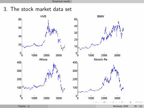
3. The stock market data set
Figure: German stock prices (daily from 1990− 2003).Fischer () Meilisalp 2009 39 / 52
Empirical results
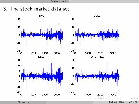
3. The stock market data set
Figure: German stock returns (1990− 2003).Fischer () Meilisalp 2009 40 / 52
Empirical results
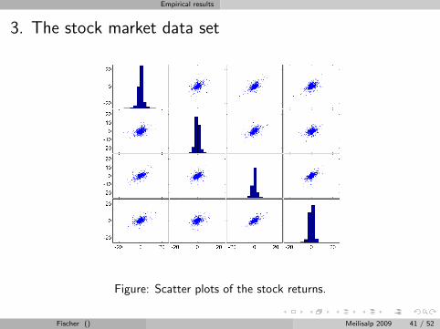
3. The stock market data set
Figure: Scatter plots of the stock returns.
Fischer () Meilisalp 2009 41 / 52
Empirical results
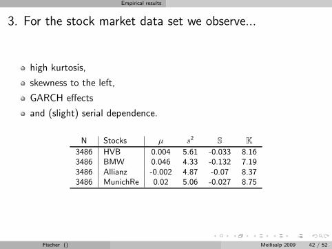
3. For the stock market data set we observe...
high kurtosis,
skewness to the left,
GARCH effects
and (slight) serial dependence.
N Stocks µ s2 S K3486 HVB 0.004 5.61 -0.033 8.163486 BMW 0.046 4.33 -0.132 7.193486 Allianz -0.002 4.87 -0.07 8.373486 MunichRe 0.02 5.06 -0.027 8.75
Fischer () Meilisalp 2009 42 / 52
Empirical results
3. Data filtering
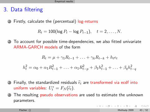
1 Firstly, calculate the (percentual) log-returns
Rt = 100(log Pt − log Pt−1), t = 2, . . . , N.
2 To account for possible time-dependencies, we also fitted univariateARMA-GARCH models of the form
Rt = µ + γ1Rt−1 + . . . + γkRt−k + htεt
h2t = α0 + α1R
2t−1 + . . . + α1R
2t−p + β1h
2t−1 + . . . + βqh
2t−q
3 Finally, the standardized residuals εt are transformed via ecdf intouniform variables: U∗
t = FN (εt).
4 The resulting pseudo observations are used to estimate the unknownparameters.
Fischer () Meilisalp 2009 43 / 52
Empirical results
3. Estimation issues
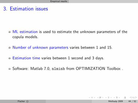
ML estimation is used to estimate the unknown parameters of thecopula models.
Number of unknown parameters varies between 1 and 15.
Estimation time varies between 1 second and 3 days.
Software: Matlab 7.0, nlminb from OPTIMIZATION Toolbox .
Fischer () Meilisalp 2009 44 / 52
Empirical results
3. Goodness-of-fit measures I
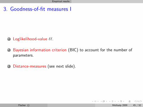
1 Loglikelihood-value ``.
2 Bayesian information criterion (BIC) to account for the number ofparameters.
3 Distance-measures (see next slide).
Fischer () Meilisalp 2009 45 / 52
Empirical results
3. Goodness-of-fit measures II
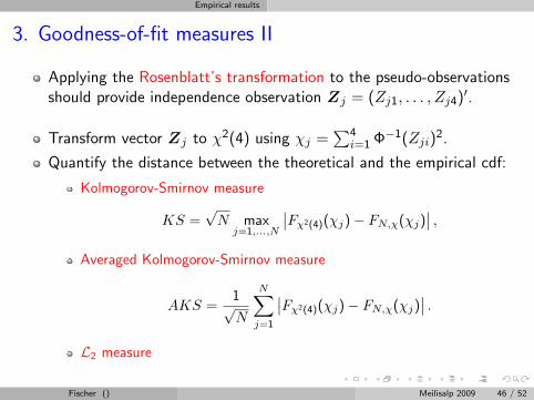
Applying the Rosenblatt’s transformation to the pseudo-observationsshould provide independence observation Zj = (Zj1, . . . , Zj4)
′.
Transform vector Zj to χ2(4) using χj =∑4
i=1 Φ−1(Zji)2.
Quantify the distance between the theoretical and the empirical cdf:
Kolmogorov-Smirnov measure
KS =√
N maxj=1,...,N
∣∣Fχ2(4)(χj)− FN,χ(χj)∣∣ ,
Averaged Kolmogorov-Smirnov measure
AKS =1√N
N∑j=1
∣∣Fχ2(4)(χj)− FN,χ(χj)∣∣ .
L2 measure
Fischer () Meilisalp 2009 46 / 52
Empirical results
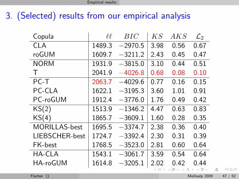
3. (Selected) results from our empirical analysis
Copula `` BIC KS AKS L2
CLA 1489.3 −2970.5 3.98 0.56 0.67roGUM 1609.7 −3211.2 2.43 0.45 0.47
NORM 1931.9 −3815.0 3.10 0.44 0.51T 2041.9 −4026.8 0.68 0.08 0.10
PC-T 2063.7 −4029.6 0.77 0.16 0.15PC-CLA 1622.1 −3195.3 3.60 1.01 0.91PC-roGUM 1912.4 −3776.0 1.76 0.49 0.42
KS(2) 1513.9 −1346.2 4.47 0.63 0.83KS(4) 1865.7 −3609.1 1.60 0.28 0.35
MORILLAS-best 1695.5 −3374.7 2.38 0.36 0.40LIEBSCHER-best 1724.7 −3392.4 2.30 0.31 0.39FK-best 1768.5 −3523.0 2.81 0.60 0.64
HA-CLA 1543.1 −3061.7 3.59 0.54 0.64HA-roGUM 1614.8 −3205.1 2.02 0.42 0.44
Fischer () Meilisalp 2009 47 / 52
Empirical results
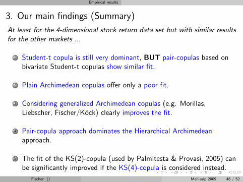
3. Our main findings (Summary)
At least for the 4-dimensional stock return data set but with similar resultsfor the other markets ...
1 Student-t copula is still very dominant, BUT pair-copulas based onbivariate Student-t copulas show similar fit.
2 Plain Archimedean copulas offer only a poor fit.
3 Considering generalized Archimedean copulas (e.g. Morillas,Liebscher, Fischer/Kock) clearly improves the fit.
4 Pair-copula approach dominates the Hierarchical Archimedeanapproach.
5 The fit of the KS(2)-copula (used by Palmitesta & Provasi, 2005) canbe significantly improved if the KS(4)-copula is considered instead.
Fischer () Meilisalp 2009 48 / 52
Empirical results
3. About that:
Our results are in line with the following study (less comprehensive)
Daniel Berg, Kjersti Aas (2008)Models for construction of multivariate dependence.Working Paper of the Norwegian Computing Center
Fischer () Meilisalp 2009 49 / 52

Empirical results
3. To conclude
Once you are forced to visit a desert island.....
don’t forget your d-variate Student-t copula!!!
Or, at least, take your bivariate Student-t copula with you...
... in order to construct pair copulas on the island.
THANK YOU FOR YOUR ATTENTION
Fischer () Meilisalp 2009 50 / 52

Empirical results
A. Backup
Fischer () Meilisalp 2009 51 / 52

Empirical results
A.1 Rosenblatt-Transformation
Start with dependent uniform vector U = (U1, U2, U3, U4)′. Define
Zi ≡ Ti(Ui) with
T1(u) = u
T2(u) = CU2|U1(u) =
∂
∂u1C(u1, u, 1, 1)
T3(u) = CU3|U2,U1(u) =
∂2
∂u1∂u2C(u1, u2, u, 1)
∂2
∂u1∂u2C(u1, u2, 1, 1)
T4(u) = CU4|U3,U2,U1(u) =
∂3
∂u1∂u2∂u3C(u1, u2, u3, u)
∂3
∂u1∂u2∂u3C(u1, u2, u3, 1)
Result is independent uniform vector Z = (Z1, Z2, Z3, Z4)′.
Fischer () Meilisalp 2009 52 / 52