modelling and identification of a one-mass system with...
TRANSCRIPT

Modelling and identification of a one-mass system
with friction
M.R.L. Kuijpers Report No. WFW 99022
Master Thesis Committee : Prof.dr.ir. J.J. Kok
Prof.clr.ir. M. Steiribuch D r h . M.J.G. van de Molengraft Dr.ir. A.G. de Jager ir. R.H.A. Hensen ir. H.J. van Leeuwen
Professor : Prof.dr.ir. J.J. Kok Coaches : Dr.ir. M.J.G. van de Molengraft
Ir. R.H.A Hensen Dr.ir. A.G. de Jager
Eindhoven, October 1999
Eindhoven University of Technology Department of Mechanical Engineering Section Systems and Control

Modelling and identification of a one-mass system with friction
M.R.L. Kuijpers
October 22 1999

Abstract
The objective of the research reported is the modelling and identification of an induction- motor driven mechanical system subjected to friction. Special attention is given to the LuGre model, a dynamic friction model, and the algorithm used during the identification of this model. The LuGre model contains the usual friction phenomena, like Coulombic and viscous friction, extended with phenomena like presliding and varying break-away forces.
The presliding and break-away phenomena are only identifiable with a high-accuracy encoder. For this purpose, a high-resolution encoder with 6.4 million counts per revolution is inst alled.
The motor is supplied with power electronics producing symmetrical three-phase voltages and currents of a fundamental frequency. The voltage and frequency of the three-phase signals are computed by an internal torque controller, which decouples the non-linear structure of the induction motor. Hence, the rotor current (and thus the torque delivered by the motor) is proportional to the input signal. Due to saturation effects in the stator coils, the assumption that the torque delivered by the motor is proportional to the input voltage is not always correct. For frequencies above the nominal frequency, the torque delivered by the motor is not proportional to the input voltage. To determine the real torque above the nominal velocity, the torque can be estimated by using an induction machine model.
Identification of this induction machine is complicated, due to the strong non-linear char- acter of the induction machine model. A less complicated model is introduced that makes the identification less difficult. In this case, the errors (energy loss by the stator coils) made by the torque controller are ascribed to a quadratic friction term (also energy loss). However, though the validation results are better with use of the non-linear induction machine model, both models describe the system with sufficient accuracy. To analyse and compare the performance of the different models, the innovation signal from the Kalman filter is a suitable tool. Using this analysis technique, the induction modei appears a much better model at high velocity (relatively small innovation) than the less complicated model (relatively big innovation).
A step by step off-line identification method is proposed to estimate both the static and dynamic model parameters associated with the LuGre and induction machine model. The step-by-step identification method uses the local identification approach, subdividing the model into smaller sub-problems, which take less effort to solve. Satisfying results are obtained using the step-by-step identification method. However, though the probability of a satisfying identification is large, the method is time consuming due to the large amount of experiments required to define the initial parameters. Finally, a Genetic Algorithm is applied, using the global identification approach where no initial parameters are required. The disadvantage of this method is that it needs very much processor time (5 days).
The system under consideration is equipped with an induction motor.
Samenvatting
De doelstelling van dit rapport is het modelleren en identificeren van een elektrisch aangedreven systeem dat onderhevig is aan wrijving. Wrijving wordt veelal gemodelleerd door Coülombse en viskeüze wïijvi~g. Met de toezeixefide wem om nog ~2xwke1wiger te ~LZ-XI~E
positioneren, beginnen wrijvings fenomenen zoals microscopisch glijden, variaties in de losbreekkracht, hysterese en het Stribeck effect een steeds grotere rol te spelen. In dit geval is een gecompliceerder model gewenst. Het LuGre model, een dynamisch op borstels gebaseerd wrijvingsmodel, beschrijft deze fenomenen. Deze dynamische wrijvings fenomenen spelen zich vooral af op microscopisch nivo en zijn niet met het blote oog noch met een gewone encoder waarneembaar. Daarom is er een encoder toegepast met een hoge nauwkeurigheid.
De identificatie experimenten zijn uitgevoerd op een robot. De aandrijving van deze robot bestaat uit een inductie motor, aangestuurd door vermogens-electronica Deze vermogens- electronica rekent het stuursignaal om naar een 3-fase spanning met een zekere amplitude en frequentie. Deze 3-fase spanning wordt zo gegenereerd dat het stuursignaal lineair is met het geleverde koppel. Hiervoor gebruikt de vermogens-electronica een statisch motormodel. Logischerwijs kan niet elk gevraagd koppel worden geleverd door de motor. Dit komt hoofdzakelijk door optredende verzadigingseffecten met name in de stator spoelen. Door het ontbreken van de terugkoppeling naar de gebruiker dat het gevraagd koppel niet wordt geleverd, worden er fouten gemaakt. Daarom is er een motormodel afgeleid dat rekening houdt met de verzadigingen en waarmee het werkelijk geleverd koppel berekent kan worden. Dit model is niet- lineair en moeilijk te identificeren. Er is daarom een ander model voorgesteld dat de energie verliezen in de statorspoelen als wrijving beschouwd dat een kwadratische verband heeft met de snelheid. Dit model is veel gemakkelijker te identificeren, maar beschrijft het systeem minder nauwkeurig.
Een stappenplan is opgesteld om zowel het wrijvings- als het motormodel nauwkeurig te kunnen identificeren (off-line). Dit stappenplan maakt gebruik van de locale identificatie methoden, waarbij het model wordt gesplitst in kleinere identificatie problemen. Door gebruik te maken van de locale identificatie methoden zoals de kleinste kwadraten methode en een Kalman filter, worden goede resultaten geboekt. Een nadeel van dit locale identificatie is dat het zeer arbeidsintensief is. Dit is te wijten aan de vele experimenten die uitgevoerd moeten worden om nauwkeurig de initieele parameters te kunnen bepalen.
Ten slotte is er een Genetisch Algoritme toegepast om het globale minimum te bepalen. Voor deze methode zijn geen tijdrovende experimenten nodig om de initieele parameters te bepalen. Het nadeel van dit algoritme is dat het veel processor tijd vergt. Het bleek dat 5 dagen niet lang genoeg was om een betere oplossing te genereren dan de resultaten verkregen met het Kalman filter.

1 Introduction 6
2 Fundamentals of friction 8 2.1 Tribology . . . . . . . . . . . . . . . . . . . . . . . . . . . . . . . . . . . . . . 8 2.2 Tribological fundamentals of frictional dynamics . . . . . . . . . . . . . . . . 9
3 Modelling of a mechanical system 11 3.1 LuGre friction model . . . . . . . . . . . . . . . . . . . . . . . . . . . . . . . . 11
3.1.1 Dynamic model behaviour . . . . . . . . . . . . . . . . . . . . . . . . . 14 3.2 Mathematical model of an asynchronous or induction machine . . . . . . . . . 20
3.2.1 Control of an induction machine . . . . . . . . . . . . . . . . . . . . . 24 3.3 Conclusions . . . . . . . . . . . . . . . . . . . . . . . . . . . . . . . . . . . . . 27
4 Identification methods 28 4.1 Least squares methods . . . . . . . . . . . . . . . . . . . . . . . . . . . . . . . 29 4.2 Extended Kalman Filter . . . . . . . . . . . . . . . . . . . . . . . . . . . . . . 30
4.2.1 Implementation Extended Kalman Filter . . . . . . . . . . . . . . . . 31 4.3 Genetic Algorithm . . . . . . . . . . . . . . . . . . . . . . . . . . . . . . . . . 31
5 Model identification 34 5.1 Static parameter estimation . . . . . . . . . . . . . . . . . . . . . . . . . . . . 36
5.1.1 Position dependent €riction . . . . . . . . . . . . . . . . . . . . . . . . 38 5.2 Mass estimation . . . . . . . . . . . . . . . . . . . . . . . . . . . . . . . . . . 38 5.3 Surveying possible friction phenomena . . . . . . . . . . . . . . . . . . . . . . 40 5.4 Static asynchronous motor parameter estimation . . . . . . . . . . . . . . . . 42 5.5 Optimisation static system in all regions . . . . . . . . . . . . . . . . . . . . . 43
5.5.1 Identification using least squares methods . . . . . . . . . . . . . . . . 44 5.5.2 Identification using EKF . . . . . . . . . . . . . . . . . . . . . . . . . . 46 5.5.3 Identification using Genetic Algorithm . . . . . . . . . . . . . . . . . . 49 5.5.4 Overview of estimated static parameters . . . . . . . . . . . . . . . . . 50
5.6 Dynamic model parameter estimation . . . . . . . . . . . . . . . . . . . . . . 51 5.6.1 Initial guess dynamic parameters . . . . . . . . . . . . . . . . . . . . . 51 5.6.2 Model validation . . . . . . . . . . . . . . . . . . . . . . . . . . . . . . 53
6 Conclusions and Recommendations 55
4

CONTENTS
A High resolution measurements 59
A.2 Interpolator . . . . . . . . . . . . . . . . . . . . . . . . . . . . . . . . . . . . . 60 A.3 Velocity determination . . . . . . . . . . . . . . . . . . . . . . . . . . . . . . . 62 A.4 Conclusion . . . . . . . . . . . . . . . . . . . . . . . . . . . . . . . . . . . . . 64
A.l Sin/cos encoder . . . . . . . . . . . . . . . . . . . . . . . . . . . . . . . . . . . 59
B Configuration of the pendulum system 65
C Data acquisition of the pendulum system 67
5

Chapter 1
Introduction
Friction is almost always present in machines with moving parts. Friction is seldom a desirable property, as it is for brakes. It is often an annoying property for servo control. Very accurate positioning and low velocity tracking is required in devices such as surgical tools, computer disk drives, assembly robots, micro manipulators, etc. The performance of many of these devices is limited by complex friction phenomena, causing tracking errors. These errors are the result of stick-slip motion, a well-known phenomenon. The main cause of stick- slip is that the friction is higher at rest than in motion. Stick-slip can be observed in a wide variety of examples, such as the screeching noise of a piece of chalk on a blackboard, earthquakes, or a violin string excited by a bow. Friction is a non-linear phenomenon, which is difficult to describe analytically. To capture its effect in mechanical systems a bristle- based dynamical model, known as the LuGre model (proposed by scientists from Lund and Grenoble) is used in this report. It captures most of the friction phenomena that have been observed experimentally, including the Stribeck effect, hysteresis, presliding and the varying break-away force. It does not capture rising static friction. To illustrate the phenomena, some important tribology aspects will be discussed in Chapter 2, followed by some fundamentals of friction dynamics.
For the purpose of identifying the springlike characteristics during stiction and the varying break-away force, etc., accurate measurements must be available. The encoder used was not satisfactory, because of the low resolution. Therefore, a sin/cos encoder is used replacing the old TTL low-resolution encoder. With use of the interpolation techniques, discussed in Appendix A, a much higher resolution can be achieved than with a TTL encoder with identical counts. Due to the reduced sensor costs, this interpolation technique is a relative cheap method to perform high-resolution measurements.
With the high-resolution encoder, measurements can be performed to identify the static and dynamic characteristics captured by the analytic LuGre friction model. A step by step off-line identification method will be proposed in Chapter 5 to estimate the nominal static and dynamic parameters associated with the LuGre and the electric motor model. This step-by- step identification method is applied to a one-mass motion system. This system consists of a rotating arm driven by an asynchronous or induction motor (both terms asynchronous motor and induction machine have the same meaning and are used interchangeable throughout this report). Detailed information about the machine can be found in Appendix B.
Usually, for control applications, a DC-motor is considered. A DC-motor has the ad- vantage that the input rotor current is proportional to the torque delivered by the motor.
6

1. Introduction
However, the system under consideration has an asynchronous motor, where the rotor current is short-circuited and is not measurable. Therefore, a torque controller decouples the non- linear structure of the asynchronous motor so that the input torque becomes proportional to the input signal. This decoupling approximates the real torque only in a restricted area (speed/torque space), where outside this area errors are made. It is attempted to improve the approximation of the torque delivered by the motor, by use of a static asynchronous model as will be discussed in Section 3.2. Therefore, the parameters of this relative complicated model have to Se estiïmted too, ? x t th is complicated bec2~se ~f the strorig no=-linear character of the model. At the end of Chapter 4 an alternative model will be given for the complicated induction machine model.
Three totally different optimisation algorithms are applied to identify the model param- eters, namely, (i) batch-wise quadratic optimisation method, (ii) an extended Kalman filter and (iii) a genetic algorithm. These algorithms will be discussed in Chapter 4. None of these seems out to be the ultimate optimisation method. Each method has an area of effectiveness. The ease of implementation often makes one identification method more preferable than the other. Also efficiency is important, but efficiency and effectiveness are considerations that are often in conflict with each other.
In Chapter 6 conclusions will be made and recommendations are given.
7
Chapter 2
Fundament als of friction
In this report we use a definition of Friction given by Hersey (1966): “Friction is the name given to the force resisting the relative motion of two bodies that are initially at rest or moving without acceleration. The friction resistance is called static friction while the bodies are at rest, otherwise it is called kinetic friction.” However, with increasing quality of measurement technology, dynamic effects can be observed, as described in this report. In order to illustrate some important friction phenomena, first some tribological aspects will be discussed.
2.1 Tribology
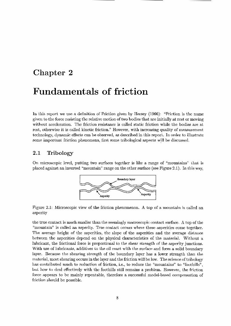
On microscopic level, putting two surfaces together is like a range of “mountains” that is placed against an inverted “mountain” range on the other surface (see Figure 2.1). In this way,
I Boundery layer I
‘Asperity I I
Figure 2.1: Microscopic view of the friction phenomenon. A top of a mountain is called an asperity
the true contact is much smaller than the seemingly macroscopic contact surface. A top of the LLmountain” is called an asperity. True contact occurs where these asperities come together. The average height of the asperities, the slope of the asperities and the average distance between the asperities depend on the physical characteristics of the material. Without a lubricant, the frictional force is proportional to the shear strength of the asperity junctions. With use of lubricants, additives to the oil react with the surface and form a solid boundary layer. Because the shearing strength of the boundary layer has a lower strength than the material, most shearing occurs in the layer and the friction will be low. The science of tribology has contributed much to reduction of friction, i.e., to reduce the L‘mountains” to “foothills”, but how to deal effectively with the foothills still remains a problem. However, the friction force appears to be mainly repeatable, therefore a successful model-based compensation of friction should be possible.
8
2. Fundamentals of friction
2.2 Tribological fundamentals of frictional dynamics
There are four regimes of lubrication in a lubricated system:
1. presliding displacement
2. boundary lubrication
3. partial finid lubrication
4. full fluid lubrication
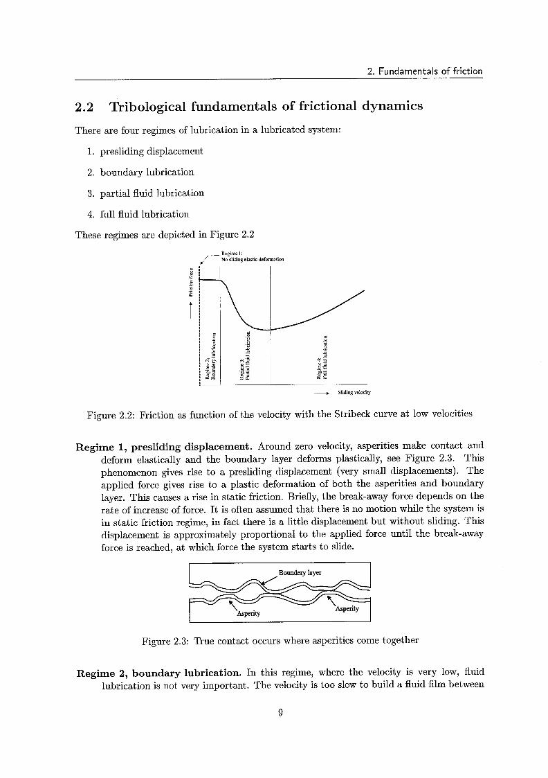
These regimes are depicted in Figure 2.2
d Sliding velocity
Figure 2.2: Friction as function of the velocity with the Stribeck curve at low velocities
Regime 1, presliding displacement. Around zero velocity, asperities make contact and deform elastically and the boundary layer deforms plastically, see Figure 2.3. This phenomenon gives rise to a presliding displacement (very small displacements). The applied force gives rise to a plastic deformation of both the asperities and boundary layer. This causes a rise in static friction. Briefly, the break-away force depends on the rate of increase of force. It is often assumed that there is no motion while the system is in static friction regime, in fact there is a little displacement but without sliding. This displacement is approximately proportional to the applied force until the break-away force is reached, at which force the system starts to slide.
Boundery layer I
Figure 2.3: True contact occurs where asperities come together
Regime 2, boundary lubrication. In this regime, where the velocity is very low, fluid lubrication is not very important. The velocity is too slow to build a fluid film between
9

2. Fundamentals of friction
Figure 2.4: Boundary lubrication. Velocity is too slow to create a fluid film.
the surfaces. This ïesülts in solid-to-solid contact of t h e b~ur,dar,ry layer, see Figure 2.4. The boundary lubricant is liable to shearing-stress. Boundary layer lubrication is a process of shear in a solid material and in this case the friction is higher than for fluid lubrication (see regime 3 and 4).
Regime 3, partial fluid lubrication As the velocity is increasing, lubricant is brought into the load-bearing region through motion. The greater the velocity, the thicker the lubricant film will be. Partial fluid lubrication arises when the film is not thicker than the height of the asperities and there still remains some solid to solid contacts, see Figure 2.5. When the film is sufficiently thick, separation is complete and the load is fully supported by fluid. Partial fluid lubrication is the most difficult of the four to model,
Figure 2.5: Partial fluid lubrication. There still remains some solid to solid contacts
because this regime is unstable. If the velocity increases in this regime, the amount of solid-to-solid contact decreases. This results in reducing the friction force and increasing of velocity of the moving surfaces. This continues until the film is sufficiently thick and no more solid-to-solid contacts occur (separation is complete). This phenomenon called “stick-slip” always occurs when there exist a negative slope in the velocity-friction plane, but can be avoided with proper control (add damping).
Regime 4, Full fluid lubrication. If the velocity is sufficiently high, solid-to-solid contact is eliminated and hydrodynamic lubrication arises, see Figure 2.6. Now, the friction force is proportional to the velocity, better known as the viscous effect.
Figure 2.6: full fluid lubrication, solid-to-solid contact is eliminated.
In section 3.1 a friction model will be discussed, that includes the tribological phenomena discussed in this chapter. Therefore, the asperities are modelled by elastic bristles.
10
Chapter 3
Modelling of a mechanical system
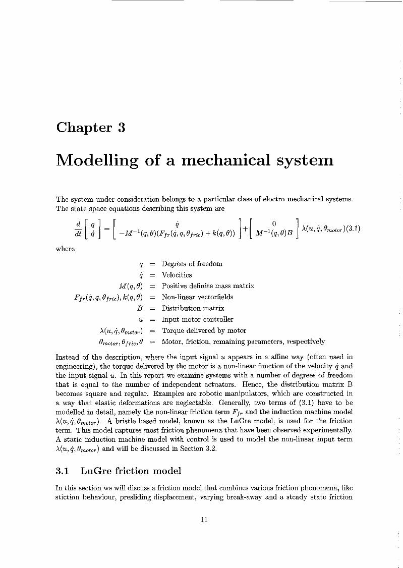
The system under consideration belongs to a particular class of eloctro mechanical systems. The state space equations describing this system are
where
= Degrees of freedom = Velocities = Positive definite mass matrix = Non-linear vectorfields = Distribution matrix = Input motor controller = Torque delivered by motor = Motor, friction, remaining parameters, respectively
Instead of the description, where the input signal u appears in a affine way (often used in engineering), the torque delivered by the motor is a non-linear function of the velocity q and the input signal u. In this report we examine systems with a number of degrees of freedom that is equal to the number of independent actuators. Hence, the distribution matrix B becomes square and regular. Examples are robotic manipulators, which are constructed in a way that elastic deformations are neglectable. Generally, two terms of (3.1) have to be modelled in detail, namely the non-linear friction term Ffr and the induction machine model X(u,q,û,,t,,). A bristle based model, known as the LuGre model, is used for the friction term. This model captures most friction phenomena that have been observed experimentally. A static induction machine model with control is used to model the non-linear input term X(u, 4, ûmotoT) and will be discussed in Section 3.2.
3.1 LuGre friction model
In this section we will discuss a friction model that combines various friction phenomena, like stiction behaviour, presliding displacement, varying break-away and a steady state friction
11
3. Modelling of a mechanical system
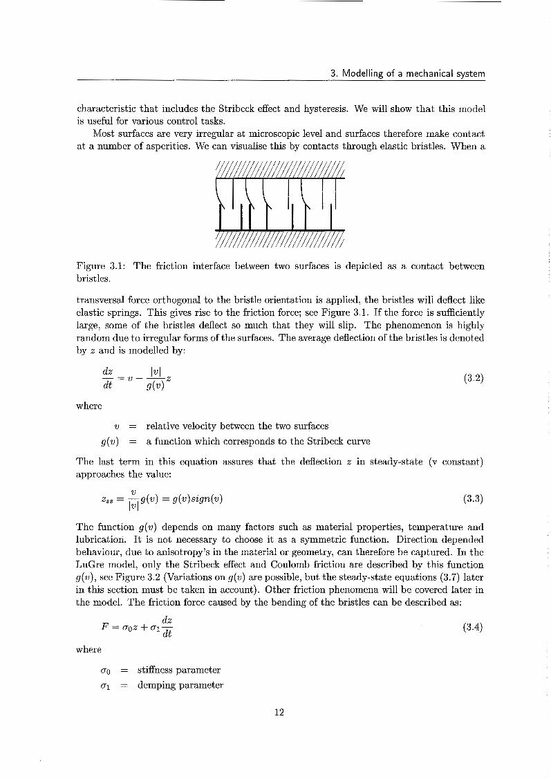
characteristic that includes the Stribeck effect and hysteresis. We will show that this model is useful for various control tasks.
Most surfaces are very irregular at microscopic level and surfaces therefore make contact at a number of asperities. We can visualise this by contacts through elastic bristles. When a
Figure 3.1: The friction interface between two surfaces is depicted as a contact between br is t les.
transversal force orthogonal to the bristle orientation is applied, the bristles will deflect like elastic springs. This gives rise to the friction force; see Figure 3.1. If the force is sufficiently large, some of the bristles deflect so much that they will slip. The phenomenon is highly random due to irregular forms of the surfaces. The average deflection of the bristles is denoted by z and is modelled by:
where
v = relative velocity between the two surfaces g(v) = a function which corresponds to the Stribeck curve
The last term in this equation assures that the deflection x in steady-state (v constant) approaches the value:
The function g(v) depends on many factors such as material properties, temperature and lubrication. It is not necessary to choose it as a symmetric function. Direction depended behaviour, due to anisotropy’s in the material or geometry, can therefore be captiired. In the LuGre model, only the Stribeck effect and Coulomb friction are described by this function g(v), see Figure 3.2 (Variations on g(w) are possible, but the steady-state equations (3.7) later in this section must be taken in account). Other friction phenomena will be covered later in the model. The friction force caused by the bending of the bristles can be described as:
dz F = CJOZ + 01-
d t where
00 = stiffness parameter 01 = demping parameter
12
(3.4)

3. Modelling of a mechanical system
-10 I I I I y , , , , -0.08 -0.06 -0.04 -0.02 O 0.02 0.04 0.06 0.08
Velocity [raas]
Figure 3.2: F'unction g(v)sign(v)
To capture other phenomena, like viscous friction, a function of the velocity can be added. In the LuGre model only viscous friction is added.
dz d t
F = O02 + O1 - + O221 (3.5)
where
02 = viscous friction parameter
The LuGre model given by (3.2) and (3.5) is characterised by the function g(v) and parameters 00, 01 and 02. In literature, the parameterisation of g(v) is often proposed as:
where
F, = Coulomb friction F, = level of stiction force v, = Stribeck velocity
With this description the model is characterised by six parameters, 00, 01, 02, F,, F, and vs. For steady state motion the following relation between friction and velocity can be written using Eqs.(3.3) through (3.6)
F&) = aog(v)sign(v) + O2V v 2
= (F, + (F, - F C ) ë ( G ) )sign(v) + 0221 (3.7)
It is important to realise that changes in velocity lead to different friction phenomena. In the following section we will discuss this behaviour.
13

3. Modelling of a mechanical system
3.1.1 Dynamic model behaviour
To get some insight in the behaviour of the LuGre Model, we substitute the LuGre model in the equations of motion, (3.1). Additionally, we assume that the input term X(u,Q,ûmotor) is linear in u and motor dynamics are neglectable. Physically, we created a mass in contact with a fixed horizontal surface. The equation of motion becomes:
(3.8)
where
q = co-ordinate of the mass or angular displacement of the inertia
01 = damping parameter 0 2 = viscous friction parameter d z - 141 - - q - - 2 dt 9 ( 4 ) u = input torque
We investigated the behaviour of this model in some typical cases, corresponding to standard experiments that were performed. In all simulations, function g ( 4 ) has been parameterised according to (3.6) and the parameters in Table 3.1 have been used. All values used are based on initial experiments discussed in Chapter 5 to create realistic simulations.
Parameter Value Unit 0 0 541 [Nm/rad] 01 2 [Nms/rad] 0 2 0.1009 [Nms/rad] Fc 0.33 [Nml Fs 0.53 [Nml v-s 0.018 [rad/s] M 0.0294 [Sg]
Table 3.1: Parameters used in simulations
Presliding displacement
In this section we will show that friction behaves like a spring with damping if the applied force is less than the break-away force. Linearising (3.2) around z = O and v = O we get
d z dq -=u=- dt d t
Inserting (3.9) in (3.8) gives:
dq2 dq M- + (01 + 0 2 ) - + 004 = u dt2 d t
(3.9)
(3.10)
It is seen that the model behaves like a system with stiffness 00 and damping 01 + 0 2 for small motions. The bristle stiffness 00 is usually very large but the damping of the LuGre model increases due to the damping term aiZ. The relative damping of this system is:
14
(3.11)

3. Modelling of a mechanical system
This shows that the linearised relative damping can be chosen arbitrarily (in simulations) by u1 regardless of the viscous friction coefficient 02. That is necessary because friction coefficient u 2 is normally not sufficiently high enough to provide good damping. In practise, there is (of course) nothing to choose for 01.
To check whether the LuGre model can capture the presliding phenomenon, we performed some simulations. During these simulations, the parameters as given in Table 3.1 are used. An external force was applied to the mass, which varied sinusoidally around zero with an arnplitfide of 9c! perce~t ~f the hre2k-2w2y ferm F, and a frequency of 0.1 raci/sec. The results of the simulation are shown in Figure 3.3. The simulation was started with zero initial conditions. The Figure 3.3 shows that this model covers the presliding phenomenon.
Figure 3.3: Presliding displacement described in LuGre model (rotation opposite clock direc- tion)
Varying break-away force
Two theories exist about the varying break-away force,
a theory which claims that the break-away depends on the dwell time (time in stick phase). How longer the systems remains in stick phase, the higher get the break-away force.
a theory which claims that the break-away depends on the rate of increase of force. Increasing the rate of force will decrease the break-away force.
Research on the role of the rate of the applied force was done by V.I. Johannes and the results pointed out that the break-away force did depend on the rate of increase of the force but not on the dwell time. Some simulations were performed using the LuGre model to determine the varying break-away force. An external force with different rates was ramped up to a one-mass motion system and when the system starts to slide the force was determined. As written in Section 3.1.1, the model behaviour in the stiction phase is essentially that of a spring with damping, and the system will move microscopically when a force is applied. The break-away force was therefore determined at the time that a sharp increase of the velocity could be observed. The force determined at break-away as function of the rate of increase of the force is shown in Figure 3.4. This phenomenon agrees with the practical experience found by V.I. Johannes. The LuGre model thus covers this break-away behaviour of real friction.
15
3. Modelling of a mechanical svstem
Figure 3.4: Break away force as function of the rate of increase of the force
Frictional lag
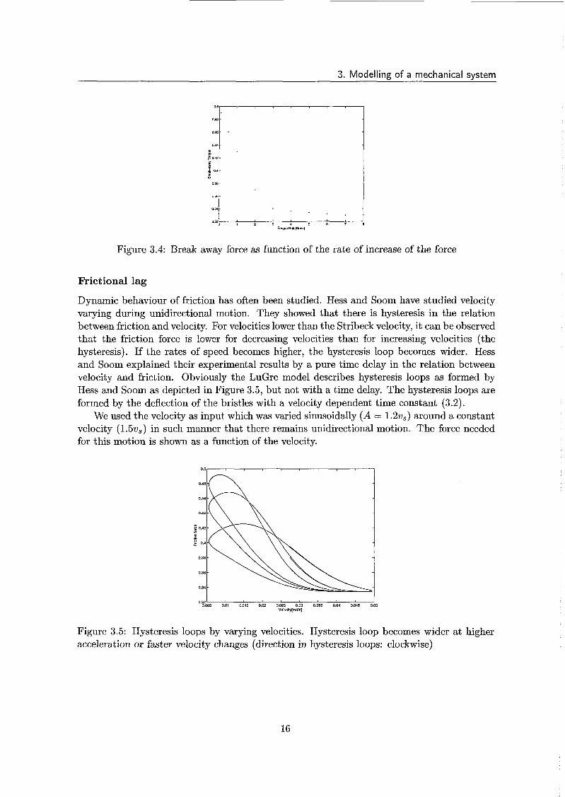
Dynamic behaviour of friction has often been studied. Hess and Soom have studied velocity varying during unidirectional motion. They showed that there is hysteresis in the relation between friction and velocity. For velocities lower than the Stribeck velocity, it can be observed that the friction force is lower for decreasing velocities than for increasing velocities (the hysteresis). If the rates of speed becomes higher, the hysteresis loop becomes wider. Hess and Soom explained their experimental results by a pure time delay in the relation between velocity and friction. Obviously the LuGre model describes hysteresis loops as formed by Hess and Soom as depicted in Figure 3.5, but not with a time delay. The hysteresis loops are formed by the deflection of the bristles with a velocity dependent time constant (3.2).
We used the velocity as input which was varied sinusoidally ( A = 1 . 2 ~ ~ ) around a constant velocity ( 1 . 5 ~ ~ ) in such manner that there remains unidirectional motion. The force needed for this motion is shown as a function of the velocity.
0.5,
0.32 0.W5 0.01 0.015 0.02 0.025 0.03 0.035 0.04 0.045
velocity[radl~] 5
Figure 3.5: Hysteresis loops by varying velocities. Hysteresis loop becomes wider at higher acceleration or faster velocity changes (direction in hysteresis loops: clockwise)
16
3. Modelling of a mechanical system
d
Stick-slip motion
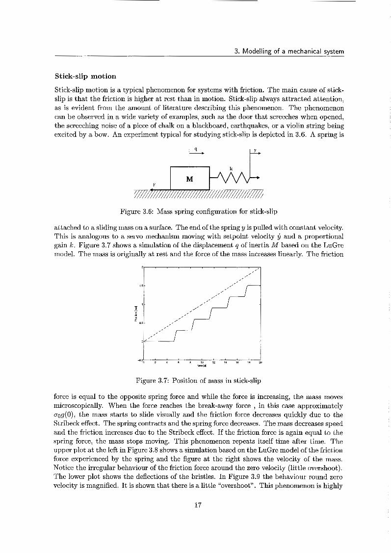
Stick-slip motion is a typical phenomenon for systems with friction. The main cause of stick- slip is that the friction is higher at rest than in motion. Stick-slip always attracted attention, as is evident from the amount of literature describing this phenomenon. The phenomenon can be observed in a wide variety of examples, such as the door that screeches when opened, the screeching noise of a piece of chalk on a blackboard, earthquakes, or a violin string being excited by a hsw. Ari experiment; typical fer studying stick-slip is depicted in 3.6. A spring is
Figure 3.6: Mass spring configuration for stick-slip
attached to a sliding mass on a surface. The end of the spring y is pulled with constant velocity. This is analogous to a servo mechanism moving with setpoint velocity y and a proportional gain k. Figure 3.7 shows a simulation of the displacement q of inertia M based on the LuGre model. The mass is originally at rest and the force of the mass increases linearly. The friction
9
, I'
O 2 4 6 8 10 12 i 4 16 i8 20 -0.5' " " " " "
time [SI
Figure 3.7: Position of mass in stick-slip
force is equal to the opposite spring force and while the force is increasing, the mass moves microscopically. When the force reaches the break-away force , in this case approximately qg(O), the mass starts to slide visually and the friction force decreases quickly due to the Stribeck effect. The spring contracts and the spring force decreases. The mass decreases speed and the friction increases due to the Stribeck effect. If the friction force is again equal to the spring force, the mass stops moving. This phenomenon repeats itself time after time. The upper plot at the left in Figure 3.8 shows a simulation based on the LuGre model of the friction force experienced by the spring and the figure at the right shows the velocity of the mass. Notice the irregular behaviour of the friction force around the zero velocity (little overshoot). The lower plot shows the deflections of the bristles. In Figure 3.9 the behaviour round zero velocity is magnified. It is shown that there is a little "overshoot". This phenomenon is highly
17

3. Modelling of a mechanical system
4.1' " " " ' " O 2 4 6 8 10 12 14 16 18 XI O 2 4 6 8 10 12 14 16 18
-011 ' ' ' ' ' ' a ' ' Time [SI Time [s]
Figure 3.8: Behaviour of LuGre model in stick-slip
dependent on the relative damping < described in (3.11). In simulation the relative damping can be chosen arbitrary by U I . < > 1 will give an over damped system. The parameterisation used in Table 3.1 gives < = 0.26. This conforms with an under-critically damped system.
5.6 5.7 5.8 5.9 6 6.1 6.2 Time [sac]
Figure 3.9: Overshoot around zero velocity,
18

3. Modelling of a mechanical system
Limit cycles caused by friction
Limit cycles could be expected in servo drives where the controller has an integral action (Figure 3.10). The stick-slip oscillation around the reference position is referred to as “hunt- ing”. Investigations of equilibrium points have been performed by Rice and Ruina(1983) and Dupont (1994). While PD-control is always stable, stick-slip can occur at low velocities. In- creasing the damping or stiffness can eliminate stick-slip. The LuGre model can cover this phenomenon as long as the operating poizt is OE the negati;-e!y sloped part of the steady state curve. In the Figures 3.10 and 3.11 limit cycles are shown resulting from a PID controller
i .4 I
Figure 3.10: Hunting in PID position control
Figure 3.11: Velocity (-), dynamic friction (- -).
kp = 3 [Nm/rad],ki = 4 [Nm/rads], kd = 3 [Nms/rad], are given for a reference step of 1 [rad]. The PID controller is implemented by
t u = K p ( 4 r - 4) - Kd(4 + Ki 1 (Qr - 4)dt (3.12)
where qr is the reference step.
19

3. Modelling of a mechanical system
3.2 Mathematical model of an asynchronous or induction ma- chine
The induction motor is the most commonly used motor. It requires practically no main- tenance. Induction machines convert electrical energy into mechanical energy by means of electromechanical induction. The principle of electromagnetic induction is that, when a con- ductor is moving across a magnetic field, a voltage is induced. If the conductor is part of a closed circuit, there wiii De a current induced. in motors, the induction principle is utilised in "reverse order": a conductor is placed in a magnetic field. The conductor is influenced by a force, which tries to move through the magnetic field. In the motor, the magnetic field is placed in the stationary part (stator). The conductors influenced by the electromagnetic forces are located in the rotating part.
The phase windings and the stator core must produce the magnetic field in a number of pole pairs. It is the number of pole pairs, which determines the speed of the rotating magnetic field (connecting the motor to AC-power supply). The speed of the magnetic field is called the synchronous speed of the motor. The phase windings consist of several coils. The number is dependent on the required pair of poles, e.g. in two pole pairs one-coil is sufficient. The magnetic field rotates in the air gap between the stator and the rotor. The magnetic field has a fixed location in the stator core, but its direction is varying. The rotational speed of the magnetic field (synchronous speed) is determined by the frequency of the power supply. With use of a three-phase supply, the magnetic fields of the individual phase windings make up a symmetrical rotating magnetic field. This magnetic field is called the rotating field of the rotor, see Figure 3.12. The amplitude of the rotating fields is constant and equal to 1.5
a b c
O" 30" 60"
Figure 3.12: Three phases gives a rotating field, the size of the magnetic field is constant
times the maximum value of the individual alternating fields (Figure 3.12). It rotates at the speed:
2 r f w, = - P
where
f = frequency of the supply voltage
20
(3.13)

3. Modelling of a mechanical system
p = number of pole pairs w, = synchronous velocity of magnetic field [rad/s]
Figure 3.12 shows the size of the magnetic fields in three different time periods. When the magnetic field vector rotates one revolution and is back to its starting point, the vector tip will have traced a complete circle.
The rotor is mounted on the motor shaft. The rotor, just like the stator, is made of thio imo sheets with shts 4s them. The rotor may be a siip ring rotor or a squirrel cage motor. These rotors differ from each other, because they have different “windings” in the slot. The slip ring rotor, like the stator, consists of wound coils, which are placed in the slots. There are coils for each individual phase, and are connected to slip rings. When the slip rings are short-circuited the rotor works like a squirrel cage rotor. The squirrel cage rotor has aluminium rods casts into the slots. At each end of the rotor the rods are short-circuited with an aluminium ring. The squirrel cage rotor is the most common type (very simple, robust and cheap) and also used in the mechanical system studied in this report. Therefore, here below, we will deal with the squirrel cage rotor only.
A rotor rod placed in the rotating magnetic field (Figure 3.13). The magnetic field of each
N
/s1
I I I I I I I I I I I I l l l l l l I I I I I I I I I I I I I I I I I I I I I I I I
/N/ Figure 3.13: induction in the rods of a squirrel rotor
pole induces 2, ciirrent io the rotor rod. The rod is thus influenced by force F . With the next pole passing, the rotor rod is of opposite polarity. This opposite polarity induces a current in a direction opposite to the first one. However, as the direction of the magnetic field has changed, the force is still affecting the rod in the same direction. When the whole rotor is placed in the rotating fields, all the rotor rods are thus influenced by forces making the rotor rotate. The rotor speed w, (asynchrsosus speed) will not reach the speed of the rotational field w, (synchronous speed) if some load is used.
The speed w, becomes:
w, = 27r-(1 f - (3.14) P
where
f = frequency of the supplied voltage p = number of pole pairs
s,,1 = relative slip
21

3. Modelling of a mechanical system
The relative slip is defined as
(3.15)
where
ws = synchronous velocity [rad/s] wr = asynchronws velocity, velocity of rotor 4, [sad/s]
In literature, the absolute slip sabs is also frequently used, defined as:
sabs = ws - wr (3.16)
In this report a clear distinction will be made between the two definitions. The force acting upon a conductor is proportional with the magnetic field @ and the
current I in the conductor. In the rotor rods voltage is induced by the magnetic field. Because of this voltage, a current I can flow in the short-circuited rotor rods. The various forces on the rotor rods make up torque (T) on the motor shaft. As the magnetic field can be considered to be constant, the torque is directly proportional with the current in the rotor.
T = k l Q 1 (3.17)
where
kl = machine parameter [m2] @ = magnetic field [TI I = current through the rotor rods [A]
But the current in the squirrel rotor is not measurable (no slip-rings). This makes the theory of the induction motor under dynamic conditions somewhat complex also because of the rotating magnetic fields. Here, a simplified form will be considered, i.e., the steady state form. The derivation is not depicted here, we confine with treating the final results. The internal torque Te as function of the slip s is approximated by the following extension (the formula of Kloss),
(3.18)
where
T e = internal torque, torque delivered by the motor[Nm]
T k = breakdown torque or the maximum torque of the motor [Nm]
~ k ( ~ ~ l ) = pull-out slip, relative slip at maximum torque
Another result of this derivation shows that the pull-out slip ~ k ( ~ ~ l ) (slip at maximum torque) is proportional with the resistance of the rotor rods. Thus s q r e ~ ) is a machine parameter.
(3.19)
22

3. Modelling of a mechanical system
where
R,(T) = rotor resistance (function of the temperature T ) [O] a = total leakage factor of the motor
X,(f,) = reactance of the rotor (proportional with frequency f , ) [O]
For identification purposes it is not interesting to know the exact sense of each machine parameter. 'l'he three parameters in (3.i9) could be joined together in one (~k(~~,)>. As the temperature of the rotor changes during operation (often the case), the rotor resistance (and Sk( re l ) ) changes also. Increasing the rotor resistance leads to increasing of the pull-out slip however the maximum torque remains unchanged. In fact this means that the torque- velocity-curve becomes stretched out. In Figure 3.14 the torque characteristic of the motor is shown. Also the stator current is shown in this plot. The rotor resistance R, is also strongly dependent on the shape of the rotor bars in combination with eddy currents through the rods (skin effect). The skin effect leads to concentration of the current in the outer portions of the conductors at higher rotor voltage frequencies, thus increasing the effective rotor resistance at higher slip (starting torque improved). Another result of the derivation of (3.18) shows
-.
generator I 4 motor drive P , Q ~~. braking area _ _ _ _ _
O ___, rotational speed (w,)
Figure 3.14: The current 11 and torque Te characteristics of an induction motor for different values of the pull-out slip sqrel) (thus for different rotor resistances)
that the maximum torque T k is proportional with the square of the supplied voltage.
3pU; (1 - a) Ti, =
4nfsxb
where
U, = stator voltage [VI f , = frequency of the stator voltage (synchronous frequency) [s-l]
x b ( f s ) = reactance of blocked rotor, proportional with frequency f s [a]
23
(3.20)

3. Modelling of a mechanical system
Considering (3.20) with use of standard three phase electrical grid properties (frequency and amplitude voltage are constant), the maximum torque T k is fixed. The only possibility to change T k is to connect a serial coil with the stator windings, in fact increasing xb. Thus increasing the maximum torque means to choose a bigger motor.
Looking at Figure 3.14, it is obvious that the normal working area of the induction machine lies between the pull-out velocity and the synchronous velocity. Only in this area a stable work-point is possible. Changing the supply voltage, the velocity could be changed in a small zïea.
3.2.1
Generally, two methods are used for controlling induction machines, namely, (i) control of an induction motor based on the steady state model and (ii) a rotor flux orientated control of current-fed induction motor. The second method has the highest dynamical performances and is of frequent use in the servo control. Nevertheless, the first method will be discussed in this report, because the servo mechanism used for experiments in this report is provided with power electronics using the first control method. The motor is supplied by a “Pulse With Modulation” (PWM) source inverter, producing symmetrical three phase voltages and currents of a fundamental frequency, see Appendix C. Shifting the synchronous velocity by varying the frequency of the supply voltage is the only possibility to change the velocity of a squirrel cage rotor in a broad range. Looking at relation (3.21) derived from [4], changing the frequency is insufficient.
Control of an induction machine
(3.21) 27r u - --fsW,@ma, “ - a
where
f, = frequency of the stator voltage (synchronous frequency)
w, = effective number of windings of one stator phase winding
Qma, = maximumflux
The flux a,,, has a maximum value due to the saturation of the magnetic circuit in the motor. With optimal use of the induction machine at nominal velocity, the maximum flux has to be reached approximately. This means that by variations frequency f,, the flux has to be kept constant on the maximum value a,,,. Using (3.21) it is obvious that it is also necessary to change the supply voltage in such way that the quotient of U, and f, reïnains constant. In fact the reference-curve shifts along the frequency axis, while maintaining its shape; this is seen in Figure 3.15. For very low velocities (3.21) is not valid, because the resistance of the stator can not be neglected anymore [4]. With frequencies above the frequency related to the nominal velocity, it is not allowed anymore to increase the supply voltage above the nominal voltage (construction demands). With the knowledge that Xr and x b are proportional with the frequency f, and with use of (3.20) new equations arise.
(3.22)
where L b and L, are constructive parameters of the motor. To derive (3.22), the following relationship is applied,
24
(3.23)
3. Modelling of a mechanical system
Torque is proportional with input (DC motor behaviour)
eed
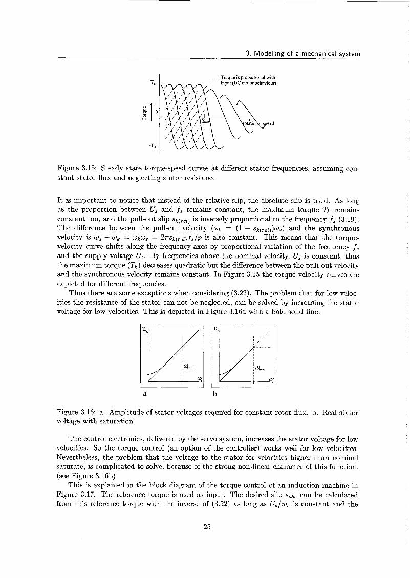
Figure 3.15: Steady state torque-speed curves at different stator frequencies, assuming con- stant stator flux and neglecting stator resistance
It is important to notice that instead of the relative slip, the absolute slip is used. As long as the proportion between U, and f, remains constant, the maximum torque T k remains constant too, and the pull-out slip s k ( r e l ) is inversely proportional to the frequency f, (3.19). The difference between the pull-out velocity (w, = (1 - s , ( ~ ~ ~ ) ) w , ) and the synchronous velocity is u, - w, = W k w , = 27r~k(~~l)f,/p is also constant. This means that the torque- velocity curve shifts along the frequency-axes by proportional variation of the frequency f s and the supply voltage U,. By frequencies above the nominal velocity, U, is constant, thus the maximum torque (T , ) decreases quadratic but the difference between the pull-out velocity and the synchronous velocity remains constant. In Figure 3.15 the torque-velocity curves are depicted for different frequencies.
Thus there are some exceptions when considering (3.22). The problem that for low veloc- ities the resistance of the stator can not be neglected, can be solved by increasing the stator voltage for low velocities. This is depicted in Figure 3.16a with--a bold solid line.
Figure 3.16: a. Amplitude of stator voltages required for constant rotor flux. b. Real stator voltage with saturation
The control electronics, delivered by the servo system, increases the stator voltage for low velocities. So the torque control (an option of the controller) works well for low velocities. Nevertheless, the problem that the voltage to the stator for velocities higher than nominal saturate, is complicated to solve, because of the strong non-linear character of this function. (see Figure 3.16b)
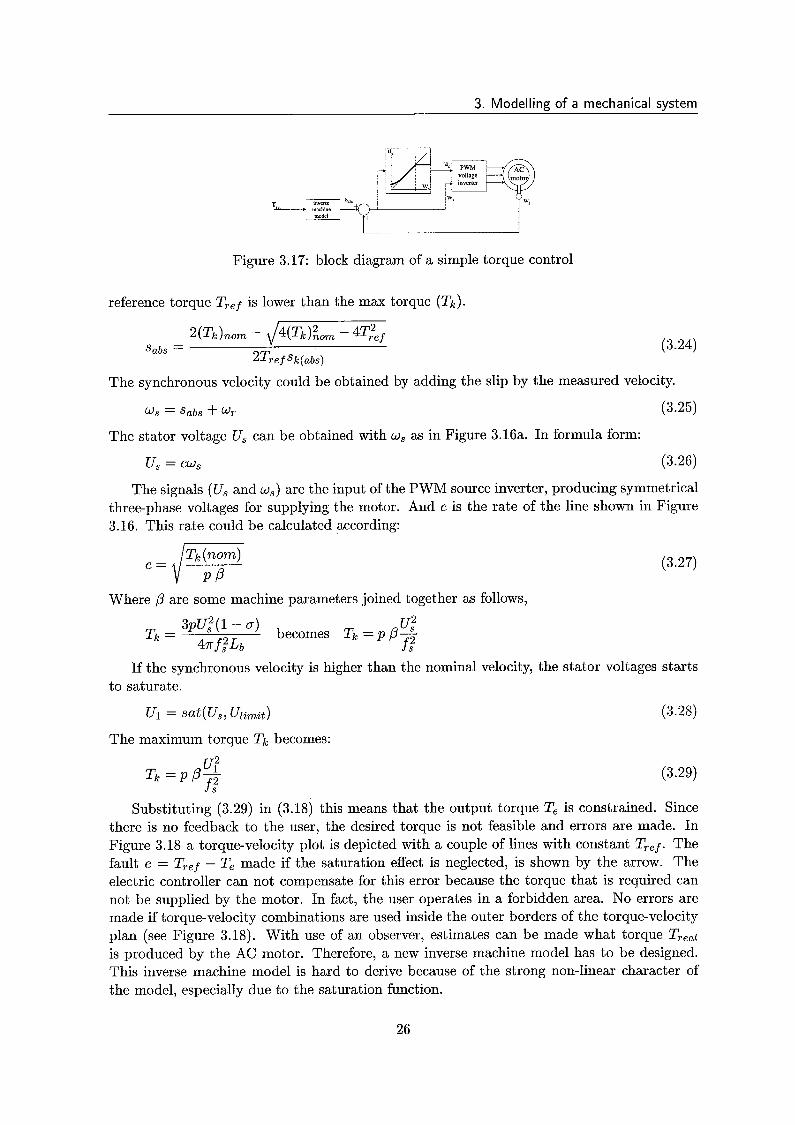
This is explained in the block diagram of the torque control of an induction machine in Figure 3.17. The reference torque is used as input. The desired slip S,bs can be calculated from this reference torque with the inverse of (3.22) as long as U,/w, is constant and the
25
3. Modelling of a mechanical system
I I
Figure 3.17: block diagram of a simple torque control
reference torque Tref is lower than the max torque ( T k ) .
(3.24)
The synchronous velocity could be obtained by adding the slip by the measured velocity.
= sabs + WT (3.25)
The stator voltage U, can be obtained with w, as in Figure 3.16a. In formula form:
u, = cw, (3.26)
The signals (U, and w,) are the input of the PWM source inverter, producing symmetrical three-phase voltages for supplying the motor. And c is the rate of the line shown in Figure 3.16. This rate could be calculated according:
(3.27)
Where ,û are some machine parameters joined together as follows,
If the synchronous velocity is higher than the nominal velocity, the stator voltages starts to saturate.
(3.28)
The maximum torque T k becomes:
T k = P P - ui2 (3.29)
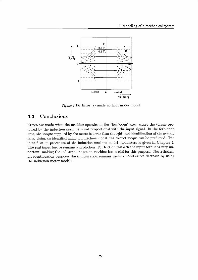
Substituting (3.29) in (3.18) this means that the output torque T e is constrained. Since there is no feedback to the user, the desired torque is not feasible and errors are made. In Figure 3.18 a torque-velocity plot is depicted with a couple of lines with constant Tref. The fault e = TTef - Te made if the saturation effect is neglected, is shown by the arrow. The electric controller can not compensate for this error because the torque that is required can not be supplied by the motor. In fact, the user operates in a forbidden area. No errors are made if torque-velocity combinations are used inside the outer borders of the torque-velocity plan (see Figure 3.18). With use of an observer, estimates can be made what torque TTeal is produced by the AC motor. Therefore, a new inverse machine model has to be designed. This inverse machine model is hard to derive because of the strong non-linear character of the model, especially due to the saturation function.
f,"
26
3. Modelling of a mechanical system
nominal 0 nominal A
velocity
Figure 3.18: Error (e) made without motor model
3.3 Conclusions
Errors are made when the machine operates in the “forbidden” area, where the torque pro- duced by the induction machine is not proportional with the input signal. In the forbidden area, the torque supplied by the motor is lower than thought, and identification of the system fails. Using an identified induction machine model, the correct torque can be predicted. The identification procedure of the induction machine model parameters is given in Chapter 4. The real input torque remains a prediction. For friction research the input torque is very im- portant, making the industrial induction machine less useful for this purpose. Nevertheless, for identification purposes the configuration remains useful (model errors decrease by using the induction motor model).
27
Chapter 4
Identification met hods
Two different methodologies in approaching identification systems exist, namely the global identification and the local identification approach. Local identification is a methodology commonly used in engineering practice. It consists of subdividing a large problem into smaller sub-problems, which take less effort to solve. Mostly all parameters used in the model have a physical meaning, resulting in a more readable model. The model describes all known physical phenomena that were applicable to the system. For complex systems this results in a very complicated model with a lot of parameters.
Global identification is a methodology where a less complicated model is supposed to describe the model. This model does not describe all physical phenomena liable to the system. Here, possible model errors are compensated by the estimated parameters which have less physical meaning than by local modelling. Not all identification methods described in this chapter can deal with the global identification approach, because of a local minimisation solution of the minimisation criteria which have multiple optima. These methods are more suitable for the local model approach. Combinations of both methodologies were commonly used (also in this report). Therefore, the purpose of this chapter is to bring together a selection of algorithms which have applications in science and engineering. We consider:
o The use of least squares methods for solving non-linear optimisation problems. This method is simpie and efficient procedure, frequently used for optimisation problems.
o The use of an Extended Kalman Filter. The Kalman filter approach has some advan- tages above the least-squares methods solving the parameter estimation problem. This is for the following reason: The Kalman filter incorporates all information that can be provided to it. It processes all available measurements regardless of their precision, to estimate the current value of the variables of interest. Therefore, the Kalman filter uses (i) the knowledge of the system and measurement device dynamics, (ii) the statistical description of the system noises, measurement errors and uncertainty in the dynamics models, and (iii) any available information about initial conditions of the variables of interest.
o The solution of optimisation problems using genetic algorithm The Genetic algorithm is useful for complicated problems and particular for those where the global maximum or minimum has to be found of a function that has many local maxima and minima. Finding of the global optimum with use of the Kalman filter approach or the Least
28
4. Identification methods
squares method is not guaranteed and is strongly dependent on the choice of the initial parameters.
It is not the intention of this chapter to describe fully the theoretical basis of these meth- ods, but to give some indication of the underlying ideas.
4.1 Least squares methods
An optimising problem involves minimising a function, i.e., the objective function, of several variables, possibly subject to restrictions on values of the variables defined by a set of con- straint functions. In this report the objective function can be expressed as a sum of squared functions.
Non-linear least squares problems give special consideration to the problem for which the function to be minimised can be expressed by the objective function. The solution of opti- misation by a single, all-purpose, method is inefficient. Optimisation methods are therefore classified into particular categories, where each category is defined by the properties of the ob- jective and constraint functions. The models described in the previous chapter are non-linear and so are the objective functions. To perform local identification, bounds on parameters are necessary (e.g., always positive values). This problem can be stated mathematically as follows:
minimise f o b j (z) ‘d z E Rn
This particular category of optimisation problems could be solved by very efficient routines developed by computing laboratories, like NAg and PORT. In this report the NAg e04fcf, PORT dn2 f bldn2gb and Matlab CONSTR routines are used. The NAg and PORT libraries are a very extensive, high quality collection of subroutines for numerical analysis, but it is more difficult to use than MATLAB since the subroutines must be called from a programming Ianguage such BS FORTRAN, BASIC 01 PASCAL.
The standard approach, used in the routines, for solving this problem is to assume an initial approximation zo and then to proceed to an improved approximation by using an iterative formula of the form:
zk+l = zk + s”k , k=0,1,2, ... (4-2)
where the vector dk is termed the direction search, and sk is the step length. The steplength 3’ is chosen so that f o b j ( z k s l ) < f o b j ( z k ) and is computed using one of the techniques for optimisation. Different techniques for non-linear least-squares optimisation are available. The distinction among these methods arise primarily from the need to use varying levels of infor- mation about derivatives of f ( z ) in defining the search direction. Most used basic techniques are the Newton-type method, the quasi type method and the conjugate gradient method. These techniques are unconstrained, which can be extended to other problem categories.
29

4. Identification methods
4.2 Extended Kalman Filter
In this section the Extended Kalman Filter (EKF) will be discussed as estimator for model parameters. The EKF can be used for optimal estimation of non-linear stochastic differential equations, general described by:
where
v( t ) =
(4.3) (4.4)
non-linear vector fields model states model inputs model outputs time state error, zero mean Gaussian noise having spectral density matrix Q ( t ) measurement error, zero mean Gaussian noise having spectral density matrix R(t)
The state errors w ( t ) and measurement errors v ( t ) are assumed to be non- correlated. The EKF is based on the minimisation of the variance of the estimation error. The derivation of how to find the minimum variance estimation is not depicted here, but can be found in Gelb [19]. We confine with treating the estimation of non-linear dynamic continuous-time systems with discrete-time measurements. In practice, this class of system is very common, because most data are acquired at a certain sampling frequency. The continuous-discrete EKF is based on the concept of recursive processing in which the measurements are utilised sequentially.
.,(t.) = a,(-) + E(I,[Xk - h,(5%(-))1 (4.5)
where
2, = estimate state at time t k
Kk = Kalman gain matrix zk = measurements
The prior estimate of the system state at time tl, is denoted by O,(-). The update is denoted by f . The gain matrix Kk is constructed in such way that it provides a minimum of the sum of the diagonal elements of the error covariance matrix P,(+).
30

4. Identification methods ~ ~~
where
Hk(&(-)) = Jacobian matrices of the non-linear model functions h(2i.1, (-))
On the interval t k - 1 5 t < t k the state estimate and integration of
2 = f (2 , u, t ) Pi t ) = I?@, u, t jF( t j + P(ijP(2, u, i) t &(i)
where
error covariance are propagated by
F ( 2 , u, t ) = Jacobian matrices of the non-linear model functions f (2) Q(t ) = spectral density error of the state error
The diagonal elements of the initial diagonal covariance matrix P(to) express the uncertainty of the initial states ? ( t o ) . Thus zero elements express infinite confidence.
4.2.1 Implementation Extended Kalman Filter
In this report, the purpose o€ using the EKF is not to estimate the state 2 ( t ) of the system but to estimate the unknown non-linear parameters 8. Expanding the state equations with the non-linear parameters, an augmented state is created. The augmented state is defined as follows
û is a vector with the same length as the amount of non-linear parameters. Considering that the non-linear parameters 8 remains constant in time, this expansion is allowed because the state equations do not change:
With this augmented state zUug, the EKF can be used as identification method. For computational and practical convenience the EKF filter is used off-line. Thus a limited amount of data (input and output) are available. Normally, this amount of data is not enough to achieve a reliable parameter estimation (parameters were not converged to constants yet). To solve this problem, an iterative EKF was designed where the same data were passed a few times through the same filter, until the parameter estimates converged. At the end of each filter pass, the final values of the parameters and the error covariance matrix which belong to the parameters P(û(t)) , were used as initial values €or the next filter pass. After each filter pass, the initial state estimates 2( t ) and the corresponding I'(?@)) gets the same value as stated at the first filter pass.
4.3 Genetic Algorithm
The basic principles of the Genetic Algorithm (GA) were inspired by the mechanism of natural selection, where stronger individuals are likely to win in a competing environment. GA uses a
31

4. Identification methods
direct analogy of such natural evolution. Through the genetic evolution method, an optimal solution can be found and represented by the final winner of the genetic game.
GA assumes that there is one solution for each problem and that the solution can be represented by a set of parameters. These parameters are encoded as the genes of a chro- mosome and can be represented by a string of values in binary form. A criterion is used to determine the fittest value (degree of “goodness”) of the chromosomes . Throughout the genetic evolution, the fitter chromosome has a bigger chance to create a better offspring, which means a, better sohtio:: t= t h e problem Ir, 2 practical GA app!ivô),im, a poplaticm pool of chromosomes has to be installed and these can be randomly set initially. The size of the population is free to choose. In each cycle of the genetic operation, a next generation is created from the chromosomes in the current population. This can only succeed if a group of these chromosomes (parents) is selected via a specific selection routine. The genes of the parents are mixed and recombined for the production of the new offspring, the next genera- tion. It is expected that from this process of evolution (manipulation of genes), the “better” chromosome will create a larger number of offspring, and thus a higher chance to survive in the following generation, simulating the survival-of-the-fittest mechanism in nature.
A “roulette wheel selection” is one of the most common techniques being used for a selection mechanism. The procedure is as follows:
o Sum the fitness of all the population members; named as total fitness (Fsum)
0 Generate a random number (n) between O and total fitness Fsum
o Return the first population member whose fitness, added to the fitness of the former population members, is greater than or equal to n.
For example, in Figure 4.1, the circumference of the roulette wheel is Fsum for all the five chromosomes. Chromosome 4 is the fittest chromosome and fills the largest interval. Chro- mosome 1 is the least fit chromosome and has a smaller interval within the roulette wheel. To select a chromosome, a random number is generated in the interval [O,Fsum] and the “pie” who spans the random number is selected.
Figure 4.1: Roulette wheel selection
This cycle of evolution is repeated until a desired termination criterion is reached (e.g. a number of evolutions, an amount of variation of individuals between the generations or a fitness criterion).
In order to make the GA evolution easier, a crossover operator and mutation operator is required. To further illustrate the crossover operation, a one point crossover mechanism is depicted in Figure 4.2. A crossover point is randomly set. The proportions of the two
32

4. Identification methods
Figure 4.2: Example of one-point cross-over
chrc~rnc~sc~rnes beyond this ciit-off pcht tc the right are to be exchsoged to form- the oEspring. An operation rate Cp,) with a typical value between 0.6 and 1.0 is normally used as the probability of crossover. After crossover, a small probability (p,) exists that one bit in the crossover switches (Figure 4.3). Mostly the mutation rate p , has a value of less than 0.1.
bit mutation 1 Figure 4.3: bit mutation of the third bit
The choice of p , and p , are strongly dependent on the optimised function. Some guidelines have been introduced in literature:
o For large population size (100) crossover rate: 0.6 mutation rate: 0.001
o For small population size (30) crossover rate: 0.9 mutation rate: 0.01
Genetic algorithm are a developing area of research and many changes could be made to the functions implemented in a genetic algorithm. For example, the roulette wheel can be implemented ir, many different ways; crossser coiild be chianged to mdti-point crosscver or to other alternatives. It will be clear that a genetic algorithm is slow in execution but it should be remembered that it is best applied to difficult problems, for example those which have multiple optima and where the global optimum is required. Since the standard algorithms often fail in these cases, the extra time taken by the genetic algorithm may be worth while.
33
Chapter 5
Model identification
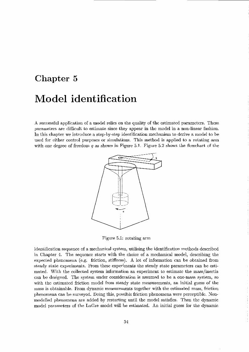
A successful application of a model relies on the quality of the estimated parameters. These parameters are difficult to estimate since they appear in the model in a non-linear fashion. In this chapter we introduce a step-by-step identification mechanism to derive a model to be used for either control purposes or simulations. This method is applied to a rotating arm with one degree of freedom q as shown in Figure 5.1. Figure 5.2 shows the flowchart of the
Figure 5.1: rotating arm
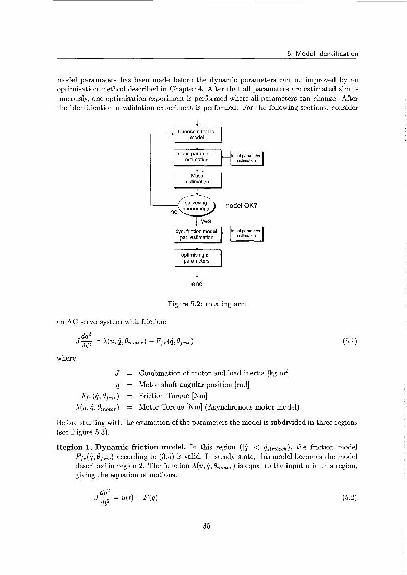
identification sequence of a mechanical system, utilising the identification methods described in Chapter 4. The sequence starts with the choice of a mechanical model, describing the expected phenomena (e.g. friction, stiffness). A lot of information can be obtained from steady state experiments. From these experiments the steady state parameters can be esti- mated. With the collected system information an experiment to estimate the mass/inertia can be designed. The system under consideration is assumed to be a one-mass system, so with the estimated friction model from steady state measurements, an initial guess of the mass is obtainable. From dynamic measurements together with the estimated mass, friction phenomena can be surveyed. Doing this, possible friction phenomena were perceptible. Non- modelled phenomena are added by restarting until the model satisfies. Then the dynamic model parameters of the LuGre model will be estimated. An initial guess for the dynamic
34
5. Model identification
model parameters has been made before the dynamic parameters can be improved by an optimisation method described in Chapter 4. After that all parameters are estimated simul- taneously, one optimisation experiment is performed where all parameters can change. After the identification a validation experiment is performed. For the following sections, consider
model
estimation estimation
p k 7 1 estimation
par. estimation
optimicing all Darameters
f
end
Figure 5.2: rotating arm
an AC servo system with friction:
dq2 Jz = X(u, 4, ernotor) - Ffr (4, e f r i c )
where
J = Combination of motor and load inertia [kg m2] q = Motor shaft angular position [rad]
Ffr (4, ûfric) = Friction Torque [Nrn] X(u, Q, Ornotor) = Motor Torque [Nm] (Asynchronous motor model)
Before starting with the estimation of the parameters the model is subdivided in three regions (see Figure 5.3).
Region 1, Dynamic friction model. In this region (141 < qstr ibech) , the friction model Ffr(4 , ûfric) according to (3.5) is valid. In steady state, this model becomes the model described in region 2. The function X(u, 4, Ornotor) is equal to the input u in this region, giving the equation of motions:
dq2 J- = u(t) - F(4) dt2
35

5. Model identification
O Stribeck nominal velocity velocity velocity +
Figure 5.3: Friction as function of the velocity, divided in three regimes
in steady-state (4 is constant):
o = u - F,,(4) (5.3)
Region 2, Static friction model. In this region (Qstribec]c < 141 < Onnominal) only the static friction model is valid (3.7), giving the equation of motions:
in steady-state (4 is constant):
0 = u - F,&) (5.5)
Region 3, Induction machine model with static friction model. In this region (141 > the static friction and induction machine model are valid. The equation of
motion is given by (5.1), the steady-state by:
In each regime the described model is dominant and could be identified separately. Because of the strong non-linear character of the models, using the separate properties leads to a better identification result (local identification).
5.1 Static parameter estimation
As described in the previous section, the static friction model is valid for the whole velocity range. To identify the static friction model, steady state experiments were performed only in regions I and 11, because in region I11 the induction machine model is also valid, mak- ing the identification of the friction model hard. The static parameters can be estimated by generating a friction-velocity plot. This plot can be measured during different constant velocity motions after the motor warm- up procedure was performed (10 minutes of turning on different velocities).
36

5. Model identification
The experiments are performed as follows. At different velocities, within a range from 4 = -2.5....2.5 [rad/s], measurements are performed at the moment that steady state is reached (velocity constant). Therefore, the closed loop system is proportional controlled with a ramp (with different rates) as reference input. The friction and velocity data values are collected by averaging the measured velocity q and input torque u over a few minutes. The static friction-velocity map is shown in Figure 5.4. The curve is not symmetric around zero. This direction dependent phenomenon can be captured to estimate parameters for both directions. To impïo-ve the idectificztioc of t h e cûeEcient F, and Fc (level of stiction force
O
oooooooooo
ooooo O
I -0.81 ' ' ' ' ' ' ' 8
-25 -2 -1.5 -1 -0.5 O 0.5 1 1.5 2 Velouv I d s 4
5
Figure 5.4: Mean static friction measured during different constant velocity motions
and Coulomb friction force respectively), data can be obtained from open-loop experiments at zero velocity (slowly ramp up the torque till the system starts to move). To fit the data, a least squares optimisation criterion, discussed in (4), is used. The following criterion must be minimised:
n
i=l
uss(4) = input torque measured during open and closed loop experiments. 4 . 2
@&) = F,sign(q) + (F, - &)ëM sign(4) + a 2 4
= a steady state model with estimated parameters
The initial values for the algorithm are estimated from Figure 5.4, which are in this case the same for both directions: Coulomb friction F: = 0.3 [Nm]; Stribeck friction F: = 0.5 [Nm]; Stribeck velocity vso = 0.1 [rad/s]; viscous friction a$ = 0.025 [Nms/rad]; All the parameters are constrained in such a way that they must be positive. In Figure 5.5 the estimated function is given together with the measured data (each circle is a measurement). It is obvious that the function does not fit very well for very low positive velocities. Expansions or changes on the steady-state model can be made to improve the minimisation (e.g. use a neural network). Therefore, it is not always necessary to give a physical explanation to the changes. For example, the Stribeck curve has no physical explanation from the tribology too. Here is supposed that an exponential function describes the Stribeck phenomena with enough
37
5. Model identification
0.6 -
0.4 -
7 0.2 - z
9 0 -
Velociiylradirl -2.5 -2 - . -
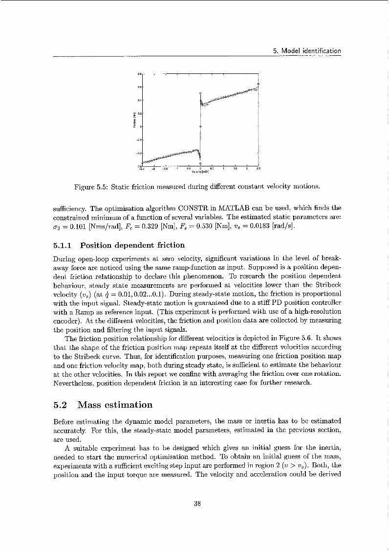
Figure 5.5: Static friction measured during different constant velocity motions.
sufficiency. The optimisation algorithm CONSTR in MATLAB can be used, which finds the constrained minimum of a function of several variables. The estimated static parameters are: 0 2 = 0.101 [Nms/rad], F, = 0.329 [Nm], F, = 0.530 [Nm], v, = 0.0183 [rad/s].
5.1.1 Position dependent friction
During open-loop experiments at zero velocity, significant variations in the level of break- away force are noticed using the same ramp-function as input. Supposed is a position depen- dent friction relationship to declare this phenomenon. To research the position dependent behaviour, steady state measurements are performed at velocities lower than the Stribeck velocity (u,) (at q = 0.01,0.02 ... 0.1). During steady-state motion, the friction is proportional with the input signal. Steady-state motion is guaranteed due to a stiff PD position controller with a Ramp as reference input. (This experiment is performed with use of a high-resolution encoder). At the different velocities, the friction and position data are collected by measuring the position and filtering the input signals.
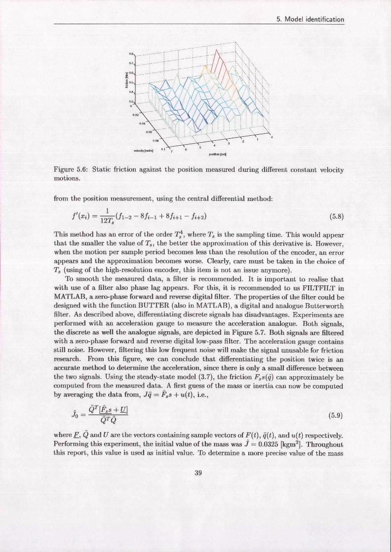
The friction position relationship for different velocities is depicted in Figure 5.6. It shows th& the shape of the friction position map repeats itself at the different velocities according to the Stribeck curve. Thus, for identification purposes, measuring one friction position map and one friction velocity map, both during steady state, is sufficient to estimate the behaviour at the other velocities. In this report we confine with averaging the friction over one rotation. Nevertheless, position dependent friction is an interesting case for further research.
5.2 Mass estimation
Before estimating the dynamic model parameters, the mass or inertia has to be estimated accurately. For this, the steady-state model parameters, estimated in the previous section, are used.
A suitable experiment has to be designed which gives an initial guess for the inertia, needed to start the numerical optimisation method. To obtain an initial guess of the mass, experiments with a sufficient exciting step input are performed in region 2 (v > us) . Both, the position and the input torque are measured. The velocity and acceleration could be derived
38
5. Model identification
P~Nim Iracli
Figure 5.6: Static friction against the position measured during different constant velocitymotions .
from the position measurement, using the central differential method :
1.f l (xi) = 12T (fl-2 - 8.fi-i + 8 fi+1 - fi+2) (5.8)
s
This method has an error of the order T,4, where Ts is the sampling time . This would appearthat the smaller the value of Ts, the better the approximation of this derivative is . However,when the motion per sample period becomes less than the resolution of the encoder, an errorappears and the approximation becomes worse. Clearly, care must be taken in the choice ofTs (using of the high-resolution encoder, this item is not an issue anymore) .
To smooth the measured data, a filter is recommended . It is important to realise thatwith use of a filter also phase lag appears . For this, it is recommended to us FILTFILT inMATLAB, a zero-phase forward and reverse digital filter . The properties of the filter could bedesigned with the function BUTTER (also in MATLAB), a digital and analogue Butterworthfilter. As described above, differentiating discrete signals has disadvantages. Experiments areperformed with an acceleration gauge to measure the acceleration analogue. Both signals,the discrete as well the analogue signals, are depicted in Figure 5 .7. Both signals are filteredwith a zero-phase forward and reverse digital low-pass filter. The acceleration gauge containsstill noise . However, filtering this low frequent noise will make the signal unusable for frictionresearch. From this figure, we can conclude that differentiating the position twice is anaccurate method to determine the acceleration, since there is only a small difference betweenthe two signals . Using the steady-state model (3 .7), the friction Fs(4) can approximately becomputed from the measured data . A first guess of the mass or inertia can now be computedby averaging the data from, Jq = Ps + u(t), i.e .,
Jo = QT QTQ ~] (5.9)
where F, Q and U are the vectors containing sample vectors of F(t), q(t), and u(t) respectively.Performing this experiment, the initial value of the mass was j = 0.0325 [kgm2] . Throughoutthis report, this value is used as initial value . To determine a more precise value of the mass
39
5. Model identification
60
40
20 - H o
2 -20 D
-40
4 0
-80
2 4 6 8 10 time [SI
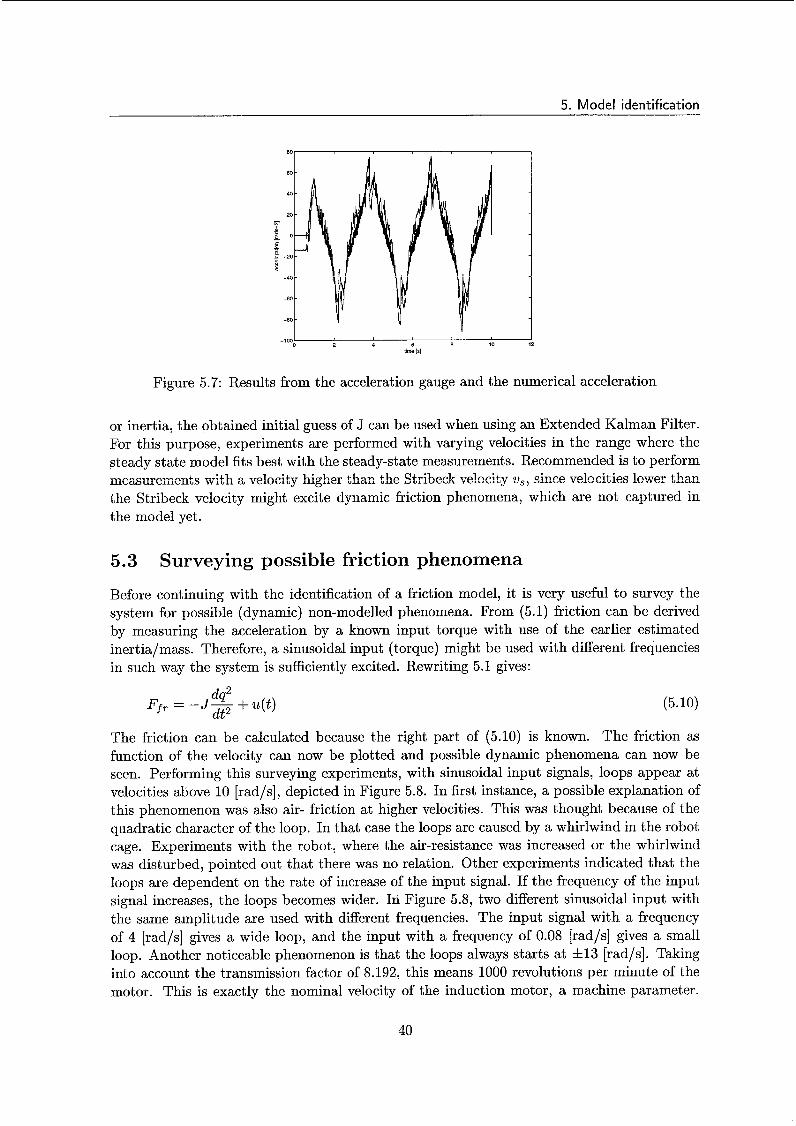
Figure 5.7: Results from the acceleration gauge and the numerical acceleration
or inertia, the obtained initial guess of J can be used when using an Extended Kalman Filter. For this purpose, experiments are performed with varying velocities in the range where the steady state model fits best with the steady-state measurements. Recommended is to perform measurements with a velocity higher than the Stribeck velocity u,, since velocities lower than the Stribeck velocity might excite dynamic friction phenomena, which are not captured in the model yet.
5.3 Surveying possible friction phenomena
Before continuing with the identification of a friction model, it is very useful to survey the system for possible (dynamic) non-modelled phenomena. From (5.1) friction can be derived by measuring the acceleration by a known input torque with use of the earlier estimated inertia/mass. Therefore, a sinusoidal input (torque) might be used with different frequencies in such way the system is sufficiently excited. Rewriting 5.1 gives:
JT = - J- dq2 + ~ ( t ) (5.10)
The friction can be calculated because the right part of (5.10) is known. The friction as function of the velocity can now be plotted and possible dynamic phenomena can now be seen. Performing this surveying experiments, with sinusoidal input signals, loops appear at velocities above 10 [rad/s], depicted in Figure 5.8. In first instance, a possible explanation of this phenomenon was also air- friction at higher velocities. This was thought because of the quadratic character of the loop. In that case the loops are caused by a whirlwind in the robot cage. Experiments with the robot, where the air-resistance was increased or the whirlwind was disturbed, pointed out that there was no relation. Other experiments indicated that the loops are dependent on the rate of increase of the input signal. If the frequency of the input signal increases, the loops becomes wider. In Figure 5.8, two different sinusoidal input with the same amplitude are used with different frequencies. The input signal with a frequency of 4 [rad/s] gives a wide loop, and the input with a frequency of 0.08 [rad/s] gives a small loop. Another noticeable phenomenon is that the loops always starts at f 1 3 [rad/s]. Taking into account the transmission factor of 8.192, this means 1000 revolutions per minute of the motor. This is exactly the nominal velocity of the induction motor, a machine parameter.
dt2
40
5. Model identification
3 -
2 -
I - - z .n 0 g
-
I -
-3
-z t -40 3 0 -20 -10 O 10 20 30 40
Velaily [mcüs]
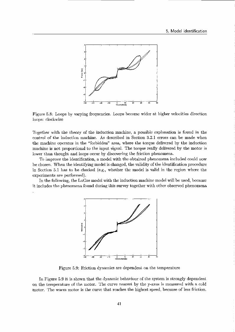
Figure 5.8: Loops by varying frequencies. Loops become wider at higher velocities direction loops: clockwise
Together with the theory of the induction machine, a possible explanation is found in the control of the induction machine. As described in Section 3.2.1 errors can be made when the machine operates in the “forbidden” area, where the torque delivered by the induction machine is not proportional to the input signal. The torque really delivered by the motor is lower than thought and loops occur by discovering the friction phenomena.
To improve the identification, a model with the obtained phenomena included could now be chosen. When the identifying model is changed, the validity of the identification procedure in Section 5.1 has to be checked (e.g., whether the model is valid in the region where the experiments are performed).
In the following, the LuGre model with the induction machine model will be used, because it includes the phenomena found during this survey together with other observed phenomena
-4 I -40 3 0 -20 -10 O IO 20 30 40
veiaitv [mdkecl
Figure 5.9: Friction dynamics are dependent on the temperature
In Figure 5.9 it is shown that the dynamic behaviour of the system is strongly dependent on the temperature of the motor. The curve nearest by the y-axes is measured with a cold motor. The warm motor is the curve that reaches the highest speed, because of less friction.
41
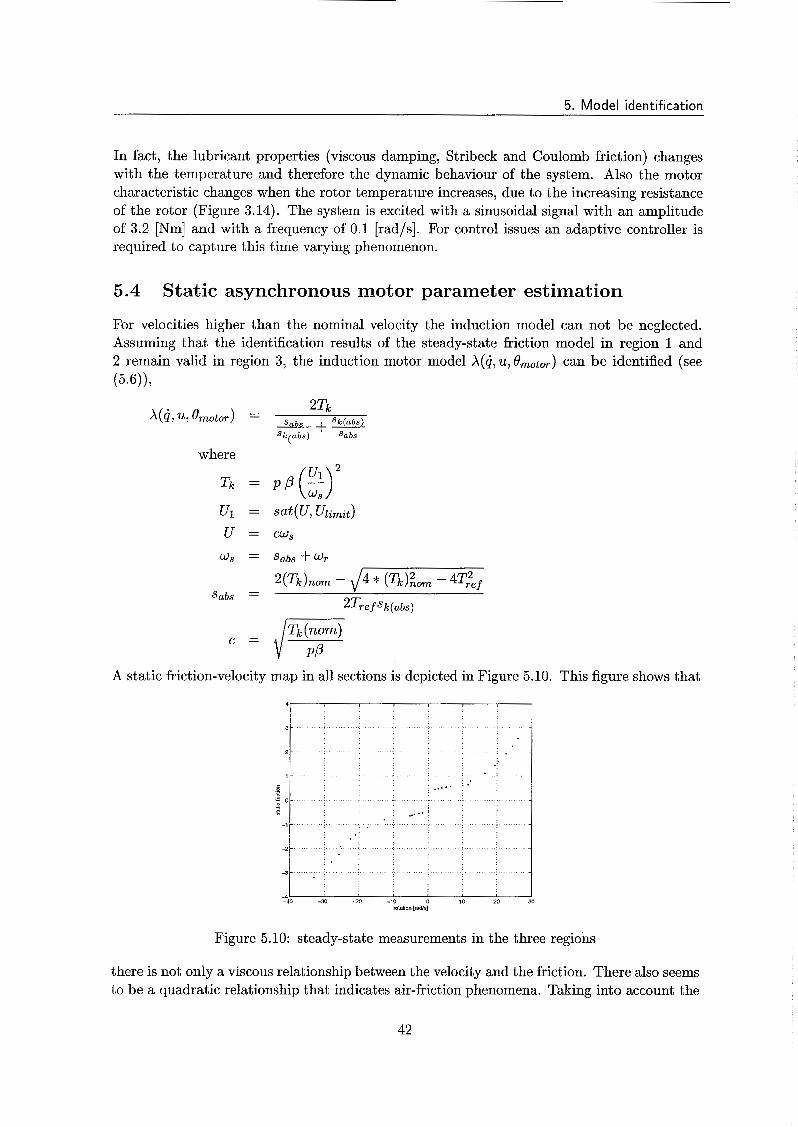
5. Model identification
In fact, the lubricant properties (viscous damping, Stribeck and Coulomb friction) changes with the temperature and therefore the dynamic behaviour of the system. Also the motor characteristic changes when the rotor temperature increases, due to the increasing resistance of the rotor (Figure 3.14). The system is excited with a sinusoidal signal with an amplitude of 3.2 [Nm] and with a frequency of 0.1 [rad/s]. For control issues an adaptive controller is required to capture this time varying phenomenon.
5.4 Static asynchronous motor parameter estimation
For velocities higher than the nominal velocity the induction model can not be neglected. Assuming that the identification results of the steady-state friction model in region 1 and 2 remain valid in region 3, the induction motor model X(Q, u, 6motor) can be identified (see (5.6) 1 7
S k ( a b s ) ' sabs
where
ws = sabs f UT
= dTk(nom) PP A static friction-velocity map in all sections is depicted in Figure 5.10. This figure shows that
Figure 5.10: steady-state measurements in the three regions
there is not only a viscous relationship between the velocity and the friction. There also seems to be a quadratic relationship that indicates air-friction phenomena. Taking into account the
42

5. Model identification
model of the induction machine, there is no quadratic relationship, but this phenomenon arises due to saturation effects in the induction machine. In Figure 5.11 the steady-state data is fit to the asynchronous model. The steady state friction is depicted by a solid line. The points are the steady state measurements. The difference between the line and the points attributes to the induction machine model. To identify the induction machine parameters, the friction parameters are fixed, where only the induction machine parameters can change. To fit these data, the following non-linear objective function has to be minimised:
2.5
Figure 5.11: Least squares optimisation induction machine parameters
(5.11)
where
$',,(o) = a steady state friction model with fixed parameters estimated in the previous fit
X(u, 4, ûmotor) = a steady state induction machine model with estimated parameters
The initial values for the algorithm were derived from machine parameters, given by the motor specifications: Ulirnit = 100 [VI, s,qabs) = 0.082 [N/s2] , (Tek)nom = 8.2 [Nm]. The parameter ,O is a mix of different parameters and for initial guess ,O = 10 is chosen. As depicted in Figure 5.11, it can be seen, that the quadratic shape of the curve (points) is transformed to the curve that consists of circles. The line is the friction model identified in region 1 ar,d 2, also used in region 3. The following parameters are the result of the minimisation: Ulimit = 98.446 [VI, ~ k ( ~ b ~ ) = 0.001 [N/s2], (Tek)norn = 3.259 [Nm] ,,O = 22.94. In the following section these parameter are used as initial values, to fit all (friction and motor model) parameters.
A
5.5 Optimisation static system in all regions
Using the estimated induction machine parameters 8motor and the estimated friction parame- ters ûfric as initial parameters for further identification methods, better identification results might be obtained. The different algorithms discussed in Chapter 4 will be applied and results wiI1 be discussed at the end of this section.
43
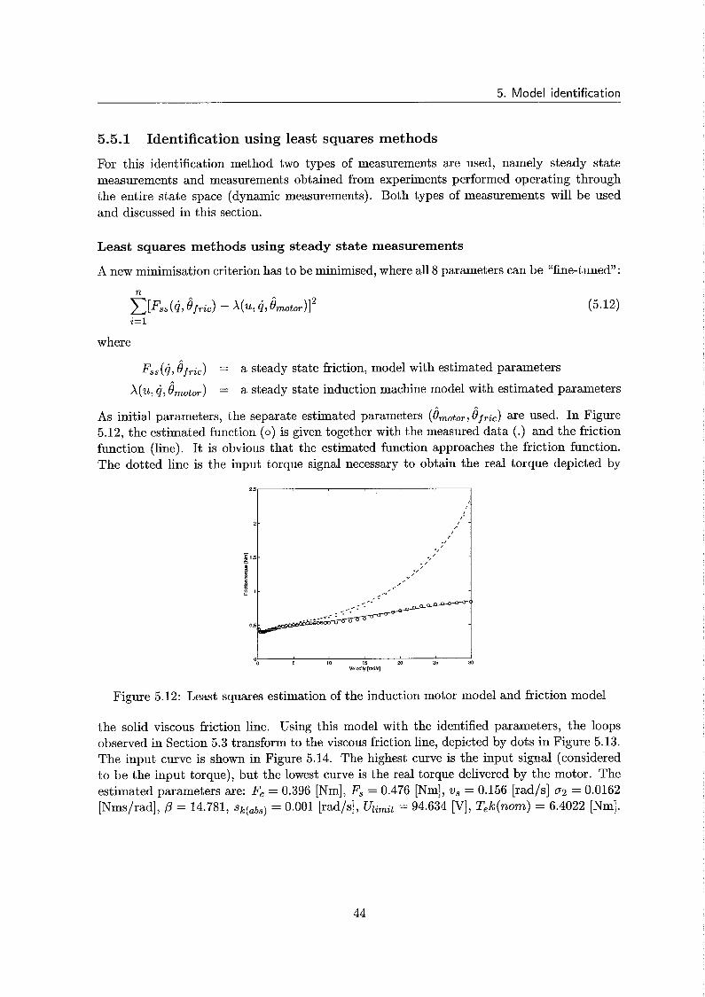
5. Model identification
5.5.1
For this identification method two types of measurements are used, namely steady state measurements and measurements obtained from experiments performed operating through the entire state space (dynamic measurements). Both types of measurements will be used and discussed in this section.
Identification using least squares methods
Least squares methods using steady state x~asuremeïìts
A new minimisation criterion has to be minimised, where all 8 parameters can be “fine-tuned”: n
(5.12) i=l
where
F,,(cj, û f r i c )
X(u, cj, ûmotor)
= a steady state friction, model with estimated parameters
= a steady state induction machine model with estimated parameters
As initial parameters, the separate estimated parameters (ernotor, af,,) are used. In Figure 5.12, the estimated function (o) is given together with the measured data (.) and the friction function (line). It is obvious that the estimated function approaches the friction function. The dotted line is the input torque signal necessary to obtain the real torque depicted by
O 5 10 15 20 25
veldhl [mas]
Figure 5.12: Least squares estimation of the induction motor model and friction model
the solid viscous friction line. Using this model with the identified parameters, the loops observed in Section 5.3 transform to the viscous friction line, depicted by dots in Figure 5.13. The input curve is shown in Figure 5.14. The highest curve is the input signal (considered to be the input torque), but the lowest curve is the real torque delivered by the motor. The estimated parameters are: F, = 0.396 [Nm], F, = 0.476 [Nm], u, = 0.156 [rad/s] 0 2 = 0.0162 [Nms/rad], f l = 14.781, S,+(&) = 0.001 [rad/s], Ulirnit = 94.634 [VI, T,k(nom) = 6.4022 [Nm].
44

5. Model identification
3
2.5
2
z 7 1.5
g 1
0.5
I 1 I
O 5 10 30 15 20 25 - O S f -5 "Siocy [ladk]
Figure 5.13: With use of the asynchronous model, the loops disappear, see dots
3
2.5
' E 2 z
g 1.5
1
0.5
"0 2 4 6 8 10 12 14 16 18 20 Time [i]
Figure 5.14: input signal, delivered torque
Least squares methods using dynamic measurements
In this section, measurements are used where the velocity changes in time (i.e., "dynamic measurements"). The minimisation criterion used differs from the previous criterion:
where
q = estimated position from model with estimated parameters x, = measured position
(5.13)
Using this criterion we confine with comparing the measured position with the results of the model (see Figure 5.15). Here, an input signal is used so that the system keeps in motion with positive velocity. The reason for that is that the induction machine model is not valid around zero-velocity (division by zero). Initial values are chosen as depicted in the previous sections. The error between the estimated and the measured data is depicted in Figure 5.15. The estimated parameters are: J = 0.0303 [kg m2], Fc = 0.3501 [Nm], F, = 0.4499 [Nm],
45

5. Model identification
m -950
J 5 10 15 20 25
bme [SI
I I
Figure 5.15: Validated complicated model with the estimated parameters using least squares estimation
v, = 0.999 [rad/s], c ~ 2 = 0.032 [Nms/rad], ,8 = 23.68, Sk(&) = 0.008 [rad/s], Ulimit = 108 [VI and (Tek)nom = 29.44 [Nm].
5.5.2 Identification using EKF
Using the EKF, the validated identification results are compared with the measured position in Figure 5.16. Figure 5.16 shows that after 20 seconds, there is an error of 3.5 [rad], a
Figure 5.16: Validated complicated model with the estimated parameters using EKF
satisfactory result. The estimated parameters are: J = 0.02754 [kg m2], F, = 0.6292 [Nm], F, = 1.283 [Nm], vs = 0.3135 [rad/s] , 0 2 = 0.0179 [Nms/rad], p = 14.63, Sk(&) = 0.0399 [rad/s], Ulirnit = 106.78 [VI and (Tek)nom = 22.25 [Nm]. To analyse the identification, the innovation signal (last term of (4.5)) of the second state is depicted in Figure 5.17 in blue together with the second propagated state estimate &(-) (red). This figure shows that the innovation signal is much smaller than the state estimate. This means that the applied model describes the system accurately. In Figure 5.18 the second state innovation signal is plotted together with the velocity (velocity divided by 500). It can be seen that during the deceleration of the system the innovation signal consequently peaks. This indicates that there is a model error, during braking. A possible explanation can be found in Figure 3.18.
46

5. Model identification
Figure 5.17: innovation signal of the EKF
Probably, the curves are not symmetrically around the torque axes . Another phenomenon canbe noticed at the break-away points . Due to the variance on the Stribeck force Fs (variance inFs is not modelled), the innovation signal give peaks . This is also noticeable at the innovationsignal of the Stribeck parameters . (not depicted here) .
Figure 5.18: innovation signal of the second state of the EKF together with the velocity
To prove that it was worthwhile to expand the model with the complicated inductionmachine model, results are depicted with less complicated models like :
. Model A, a mechanical system with Coulomb and viscous friction without inductionmachine model (T = u) . The validation results are given in Figure 5 .19. The estimatedparameters are J = 0.044736 [kg m2], Q2 = 0.0764 [Nm] and F, = 0 .2275 Nm
. Model B, The same model as Model A, expanded with the Stribeck effect and a quadraticvelocity term. The validation results are shown in Figure 5 .20 . The final estimatedparameters are: J = 0.0499 [kg m2], v2 = 0.0141 [Nms/rad], F, = 0.677 [Nm], Fs =2 .178 [Nm], vs = 0.067 [rad/s] and U3 = 2 .95210-3 [Nms/rad2]
The validation of model A is not satisfying (larger errors) . More satisfying are the identi-fication results of model B . Comparing the errors of model B (Figure 5 .20) with the errors
47
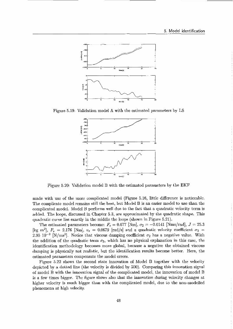
5. Model identification
I 5 10 15 20 25
-1WO
time [rl
5 10 15 20 25 üme [SI
-20
Figure 5.19: Validation model A with the estimated parameters by LS
a=-
- i
I 5 10 15 20 25
-1WJ
Pme [s]
I I O 5 10 15 20 25
Pms[9]
Figure 5.20: Validation model B with the estimated parameters by the EKF
made with use of the more complicated model (Figure 5.16, little difference is noticeable. The complicate model remains still the best, but Model B is an easier model to use than the complicated model. Model B performs well due to the fact that a quadratic velocity term is added. The loops, discussed in Chapter 5.3, are approximated by the quadratic shape. This quadratic curve lies exactly in the middle the loops (shown in Figure 5.21).
The estimated parameters become: F, = 0.677 [Nm], 02 = -0.0141 [Nms/rad], J = 25.3 [kg m2], F, = 2.176 [Nm], o, = 0.0679 [rad/s] and a quadratic velocity coefficient 03 = 2.95 [N/ms2]. Notice that viscous damping coefficient 02 has a negative value. With the addition of the quadratic term 03, which has no physical explanation in this case, the identification methodology becomes more global, because a negative the obtained viscous damping is physically not realistic, but the identification results become better. Here, the estimated parameters compensate the model errors.
Figure 5.22 shows the second state innovation of Model B together with the velocity depicted by a dotted line (the velocity is divided by 500). Comparing this innovation signal of model B with the innovation signal of the complicated model, the innovation of model B is a few times bigger. The figure shows also that the innovation during velocity changes at higher velocity is much bigger than with the complicated model, due to the non-modelled phenomena at high velocity.
48

5. Model identification
2.5
2-
E 1.5- z
Y I -
0.5
-
-
j .....
... .... .. , . ...
/::: .. . . . . . . . . . . . .
. . . . . . . . . ...... , .. ,
O t
O 5 10 15 20 25 - O S 1 -5 vebsity [iadk]
Figure 5.21: Quadratic curve is lies exactly in the middle of the loops
0.05
0.04
0.03
N s 0.02
.6 g 0.01
I
O
-0.01
-0.02
Figure 5.22: Innovation of the second state of the EKF (model B)
5.5.3 Identification using Genetic Algorithm
in this chapter the genetic algorithm is applied io estimate the static parameters. The genetic algorithm searches the global maximum of the following objective function.
* n
(5.14)
where n
q(u, Ornotor, O f r i c ) = estimated position from model with estimated parameters
z, = measured position N = number of data points
The chromosome was performed by binary string. The amount of bits is dependent on the bounds and the desired precision of the binary string. One-point crossover and bit mutation are applied with operation rates of 0.6 and 0.05, respectively. The population size is set to 10 and 100 generations are evaluated. Due to the stiffness of the problem and limited computational time, The measuring data is increased from 20 till 12 seconds. Nevertheless,
49

5. Model identification
this results in a total identification time of 96 hours. The results are depicted in Figure 5.23. This figure shows a good fit, however the identification performed with a Kalman filter fits
I 10 12 14 18 20 15
time [y
Figure 5.23: validate model with the parameters estimated by the GA
better. Probably, the objective function convergences better after more generations. The final identification parameters (parameters with the best fitness) are: J = 0.0329 [kgm2], F, = 0.5701 [Nm], F, = 0.449 [Nm], vs = 0.0225 [rad/s], 02 = 0.0580 [Nms/rad], = 39.816, sqabs) = 0.0613 [Nms/rad], Uzirnit = 133.1664 [VI and (Tek)nom = 38.1664 [Nm]. The optimisation is performed by simulations based on MATLAB with a genetic toolbox [18]. The objective values of the best chromosome in the pool against generations are depicted in
o
Figure 5.24: Objective function vs. generations
Figure 5.24. It shows that starting from the initial population the algorithm develops new generations which rapidly explore the region of interest.
5.5.4
In Table 5.1 an overview of the obtained estimated parameters is given. Also the initial parameters are given, used for the Least square methods and the Kalman filter. The final results from the three different optimisation methods are given in Table 5.2 To obtain a fair comparison between the different models, from each model the norm of the error vector is divided by the length N of the vector. Applying the LQ en EKF optimisation, the same initial parameters are used. The GA needs no initial parameters (only bounds of the parameters).
Overview of estimated static parameters
50
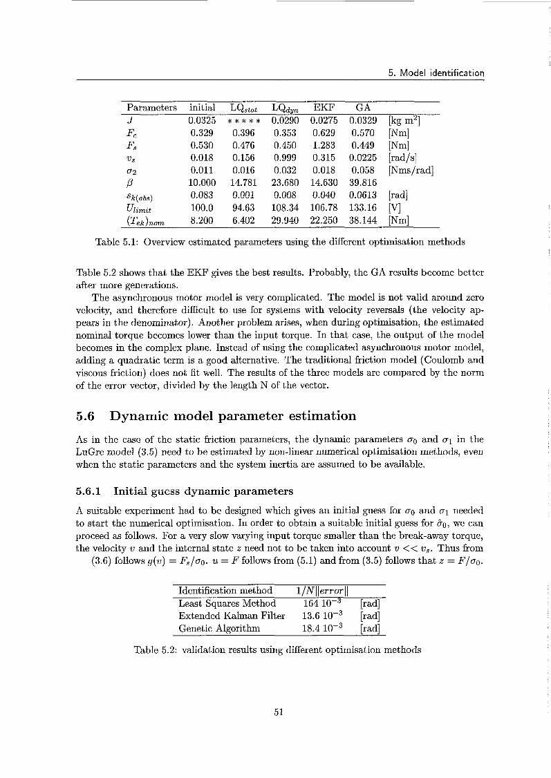
5. Model identification
Parameters initial LQstat LQdyn EKF GA J 0.0325 * * * * * 0.0290 0.0275 0.0329 [kg m2]
0.329 0.530 0.018 0.011 10.000 0.G8.3 100.0 8.200
0.396 0.476 0.156 0.016 14.781 0.001 94.63 6.402
0.353 0.450 0.999 0.032 23.680 0.008 108.34 29.940
0.629 1.283 0.315 0.018 14.630 0.040 106.78 22.250
0.570 [Nm] 0.449 [Nm] 0.0225 [rad/s] 0.058 [Nms/rad] 39.816 0.0613 [rad] 133.16 [VI 38.144 [Nm]
Table 5.1: Overview estimated parameters using the different optimisation methods
Table 5.2 shows that the EKF gives the best results. Probably, the GA results become better after more generations.
The asynchronous motor model is very complicated. The model is not valid around zero velocity, and therefore difficult to use for systems with velocity reversals (the velocity ap- pears in the denominator). Another problem arises, when during optimisation, the estimated nominal torque becomes lower than the input torque. In that case, the output of the model becomes in the complex plane. Instead of using the complicated asynchronous motor model, adding a quadratic term is a good alternative. The traditional friction model (Coulomb and viscous friction) does not fit well. The results of the three models are compared by the norm of the error vector, divided by the length N of the vector.
5.6 Dynamic model parameter estimation
As in the case of the static friction parameters, the dynamic parameters PO and 01 in the LuGre model (3.5) need to be estimated by non-linear numerical optimisation methods, even when the static parameters and the system inertia are assumed to be available.
5.6.1 Initial guess dynamic parameters
A suitable experiment had to be designed which gives an initial guess for 00 and 01 needed to start the numerical optimisation. In order to obtain a suitable initial guess for 60, we can proceed as follows. For a very slow varying input torque smaller than the break-away torque, the velocity w and the internal state x need not to be taken into account w << w,. Thus from
(3.6) follows g(w) = F,/ao. u = F follows from (5.1) and from (3.5) follows that z = F/Q.
Identification method l/Nll error 1 1 Least Squares Method 164 10V3 [rad] Extended Kalman Filter 13.6 [rad] Genetic Algorithm 18.4 [radl
Table 5.2: validation results using different optimisation methods
51

5. Model identification
Model Complicated model 13.6 [rad]
i / N 1 ) emor I(
Model A 119 [rad] Model B 20.7 [radl
Table 5.3: validation result by different models
Substituting above expressions in (3.2) gives:
(5.15)
Using an input ramp with u(t) = et, with c very small and c > O, (5.15) can be explicitly integrated for zi > O;
(5.16)
The normally not measurable state z can now be obtained in a time interval (O, T ) and a first guess for 80 can be computed by averaging these data, u(t) = oox(t), i.e.,
ZTU ZTZ
O0 = - (5.17)
where Z and U are the vectors containing sample vectors of z ( t ) and u(t) respectively. Using an input ramp function u(t) = ct with c = 0.005. The response of the system is depicted in Figure 5.25. Integrating (5.16) gives a first guess for 30. In this case 30 = 3339 [Nm/rad].
I O 1 2 3 4 5 6 7 8
lime [SI -0.51
Figure 5.25: Response system on a slow ramp input (magnified)
In the Figure 5.26, the break-away point is very obvious (&8 [s]). Until break-away occurs, the integrating expression can be used. The presliding movements shown in Figure 5.25 are neither perceptible with bare-eye, nor measurable without the high-resolution encoder. The technique behind the high-resolution encoder is discussed in Appendix A. Figure 5.25 is a very magnified version of Figure 5.26. An initial guess for 01 can be obtained by linearising (5.1) and 3.5 for very small displacements in the stiction regime. In that case x N q and the linearised description becomes:
d2q dq J- + (01 + o2)- + ooz = u(t) dt2 d t
52
(5.18)

5. Model identification
2.2
z * 2 - =
4 . 8 -
1.6
1.4-
1.2
I 2 4 6 8 10 12
time [mq
-
-
A A -
Figure 5.26: Response system on a slow ramp input
With an open loop step input, an initial guess for 60 can be obtained by matching its response to the system position measurements. The magnitude of the step input must be chosen ap- proximately around 80% of the break-away force F,. Using a step input of 0.4.. . O [Nm], results in Figure 5.27. Here another problem arises to estimate the damping. To estimate the initial bristle damping, the frequency of the overshoot can be used. Nevertheless, this frequency is not accurate because one period is depicted by only 5 samples, too few for depict- ing a fluctuating signal uniquely. Using (3.10, the undamped frequency could be determined. This frequency is lower than the figure shows. Probably, the vibrations depicted in the fig- ure may be due to elastic deformations in axle to sensor. Guessed is a bristle damping of 4 [Nms/rad] .
Figure 5.27: Response system on a step input below the break-away force
5.6.2 Model validation
Finally, when all initial parameters are known, the parameters can be refined by an opti- misation algorithm. Identification of the dynamic friction model is difficult, due to the stiff character of the friction dynamics. Some identification methods are also less useful, because
53
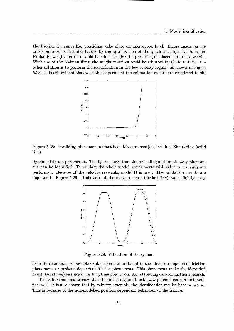
5. Model identification
the friction dynamics like presliding, take place on microscope level. Errors made on mi- croscopic level contributes hardly by the optimisation of the quadratic objective function. Probably, weight matrices could be added to give the presliding displacements more weight. With use of the Kalman filter, the weight matrices could be adjusted by Q, R and Po. An- other solution is to perform the identification in the low velocity regime, as shown in Figure 5.28. It is self-evident that with this experiment the estimation results are restricted to the
O 2 0.4 0.6 0.8 1 I .2 Time IS1
-0.m
Figure 5.28: Presliding phenomenon identified. Measurement (dashed line) Simulation (solid line)
dynamic friction parameters. The figure shows that the presliding and break-away phenom- ena can be identified. To validate the whole model, experiments with velocity reversals are performed. Because of the velocity reversals, model B is used. The validation results are depicted in Figure 5.29. It shows that the measurements (dashed line) walk slightly away
Figure 5.29: Validation of the system
from its reference. A possible explanation can be found in the direction dependent friction phenomena or position dependent friction phenomena. This phenomena make the identified model (solid line) less useful for long time prediction. An interesting case for further research.
The validation results show that the presliding and break-away phenomena can be identi- fied well. It is also shown that by velocity reversals, the identification results become worse. This is because of the non-modelled position dependent behaviour of the friction.
54

Chapter 6
Conclusions and Recommendat ions
The choice of materials and lubricants has a large influence on friction behaviour of machines. When reducing friction is desired, it is preferred to start with the design of the machine. When for some reasons, e.g., costs of high precision techniques, friction is still significant, control strategies have to be developed reducing the friction problems. Different control strategies varying in complexity are possible. Therefore the control engineer needs suitable friction models. For control tasks in regimes of high velocity, a simple friction modei incorporating only viscous friction forces may be sufficient in most cases. However, with the system under consideration, description of high-velocity behaviour with only viscous friction is not optimal. In the high velocity regime, the non-linear induction machine effects are dominant, transform- ing the input torque to a lower torque than asked for by the controller. A model is derived that describes this phenomenon, but this model is very complicated and hard to identify. Ex- periments with a simpler model incorporating a viscous and a quadratic friction force, is also sufficient. In this case, the errors (the energy loss by saturation of the stator coil) made by the torque controller are ascribed to a quadratic friction term (also energy loss). Comparing both methods, by adding the quadratic friction term to the model, good validation results are obtained. However the validation results are better with use of the non-linear induction machine model.
On the other hand, when high precision position control or tracking at low velocity is required, phenomena such as the stick-slip varying break-away force and the Stribeck effect will be important. In this case a more comprehensive friction model is required. The LuGre model describes various friction phenomena iike stiction behaviour, varying break-away, the Stribeck effect and frictional lag. The LuGre model is based on deflecting viscous elastic bristles. When applying a force, the bristles will deflect like springs. If the force is sufficiently large, the bristles will slip (break-away). The presliding and break-away phenomena are only measurable with a high-resolution encoder.
Three types of identification methods are used, the batch-wise least-squares method, the Kalman filter and the Genetic Algorithm. The Kalman filter approach differ from the batch- wise least-squares method for the following reasons: (i) the Kalman filter takes explicitly in account the model and measurements uncertainties,(ii) the Kalman filter takes measurements in account incrementally (recursively), (iii) the Kalman filter can take in account a priori information, (iv) the Kalman filter incorporates all information that can be provided.
The genetic algorithm differs from the other search procedures since it involves two spe- cial features to get the global optimum: crossover and mutation. Starting from a random
55
6. Conclusions and Recommendations
initial population, the algorithm develops new generations that rapidly explore the region of interest. This is useful for complicated optimisation problems, like the identification of the induction machine model, and in particular for those where the global maximum or mini- mum has to be found of a function that has many local maxima and minima. In that case standard optimisation methods like, Newton, Quasi Newton and conjugate gradient method can only find the local minimum. Identification results show that the friction parameters are approximately equal to each other, independent of the used identification method. However, bile estimated rlotoï pararnetera &Eer per ideGti6cation meth~d. The abtained identiEc2tim results, with relation to finding the global minimum, of the Least squares method and the Kalman filter are dependent on the initial parameters. To obtain accurate initial parameters, suitable experiments are designed.
However a genetic algorithm may locate the global optimum, although this is not guar- anteed within finite time. Starting from the initial population, the algorithm develops new generation which rapidly explore the region of interest. Nevertheless it is time consuming to find an accurate minimum in this region. Therefore it is recommended to combine the genetic algorithm with the Kalman filter or Least squares approach, where the initial parameters are obtained by the genetic algorithm.
Besides considerations of effectiveness, also the ease of implementation often makes an estimation method more preferable than the other. The genetic algorithm is the easiest method to implement, whereas an objective function must be generated together with the matrix with bounds of the region of interest.
The quadratic minimisation methods need, beside the objective function and the bounds, also some initial conditions. To obtain good identification results, initial parameter estimation experiments have to be performed. Initial parameter experiments are time consuming. Using the Kalman filter algorithm, also an objective function is required. Depending on the solver, the Jacobian of the in- and output models must be derived. Giving the initial parameters, also the confidence of the initial parameter must be estimated together with the confidence in the models and measurements. A lot of variables, responsible for the performance of the algorithm, have to be adjusted accurately. Once a good adjustment is found, very good results are obtained.
Problems of numerical stiffness can be expected, using the LuGre friction model, because presliding displacements take place on a different time scale than other phenomena.
Due to the fact that the real torque delivered by the motor is an approximation, the robot system is less useful for friction research. An easier and perhaps more acciirate way to get the real delivered torque is to measure it with a torque gauge. For control application, the robot is still very useful. This report gives two alternatives to model the system approximately. Using friction compensation techniques, position depended friction must be added to the control algorithm. Modelling and identifying this position dependent friction is an interesting case for further research.
A L
56

Bibliography
[i] Armstrong-Hélouvry B., Dupont P., and Canudas de Wit C., “A survey of models, analysis tools and compensation methods for the control of machines with friction”, Automatica, 30, 1083-1138, (1994).
[2] Prof Dr.-Ing. Werner Leonhard, “Control of Electrical Drives”, Springer-Verslag Berlin Heidelberg New-York Tokyo, (1985).
[3] Irving. M. Gottlieb, “Electric Motors and Control Techniques”, 2nd edition, TAB Books Divisions of Mc Graw-Hill Inc., (1994).
[4] Ir. D. Hamels, “Elektrische aandrijftechniek”, Stenfert Kroese Uitgevers, (1992).
[5] K.F.Man, K.s. Tang, S. Kwong and W.A.Halang, “Genetic algorithms for control and signal processing.”, Advances in Industrial control, Springer verslag Berlin Heidelberg, New-York, (1997).
[6] R.H.A Hensen, “Extended Kalman Filter based Identification Tool”, Report No. WFW 99.003, Eindhoven University of technology (TUE), (1999).
[7] G.Lindfield and J.Penny, “Numerical Methods Using MATLAB.”, Ellis Horwood Lim- ited, (1995).
[8] Nag Ltd, NAg Fortran library Introduction guide, Mark 18 Printed and produce by NAg
[9] C. Canudas de Wit, H. Olsson, K.J. Astrom, P.Lischinsk, “A new model for control of systems with friction.”, IEEE Transactions on automatic control, 40(3), 419-425, (1995).
[IO] C. Canudas de Wit, P. Lischinsky, “Adaptive friction compensation with partially known dynamic friction model.”, IEEE contol and signal processing, 11, 65-80, (1997).
[li] R.H.A. Hensen, G.Z.Angelis, M. J.G. van de Molengraft, A.G. de Jager, J. J.Kok., “Grey- box modeling of friction: An experimental study.”, Eindhoven Universtity of technology, Faculty of Mechanical Engineering, (1997).
[12] Friedhelm Altpeter, Fathi Ghorbel Roland Longchamp, “A singular pertubation analy- sis of two friction models applied to a vertical EDM-AXIS” , Dept. of Mechanical Engr., Rice University, Houston, USA.
[13] Magnus Gaffert, “Comparisons of two dynamic friction models.”, Proceedings of the 1997 IEEE international Conference on Control applications, Hartford, 386-391, (1997).
57

BI B LIOGRAPHY
D. A. Heassig, Jr. B. Friedland, “On the modeling and simulation of friction”, ASME Journal of Dynamic System, Measurement, and Control, September 1991, 113, 354-362
C. Canudas de Wit, “Control of Friction-driven Systems”, Laboratoire d’Automatique de Grenoble, ECC’99 congress. 1-6.
P.Lischinsky, C.Canudas de Wit, G.More1, “Friction Compensation of a schilling hy- draulic robot”, Proceedings of the 1997 IEEE international conference on Control Ap- plications, Hartford, 294-299, (1993).
H.versteeg H. Nijmeijer, “Friction in robots models and control policies”, A literature overview, Enschede, (1995)
C.R. Houck, J.A. Joines and M.G. Kay, “A genetic algorithm for function”, ACM Transactions on Mathematical Software, (1996).
A.Gelb and J.F.Kasper, “Applied Optimal Estimation”, The Analytic Sciences Corpo- ration.
58

Appendix A
High resolution measurements
To measure dynamic friction phenomena, some experiments have to be done with a high- resolution encoder (The encoder formerly used has a resolution of 32.768 increments per revolution, corresponds with 191,7,urad). To perform a high-resolution encoder, an encoder is used with an exact sin-wave signal as output instead of the common used square-wave pulse encoders(TTL-encoders). To interpolate the output sine-wave signal with a higher degree, a much higher resolution TTL signal is obtainable. With this technology, f6 .55 million increments per revolution are obtained, this corresponds with 0.96 [,u rad], an improvement of a factor 200. The principle of interpolation is shown in Figure A.l In the following sections,
sinicos TTL
Figure A. 1: Principle of interpolation sinusoidal signals (interpolation grade = 8)
the working of the sin/cos encoder and the interpolator is discussed more detailed.
A . l Sin/cos encoder
Interpolation of sine-wave signal with high accuracy is only possible if the sinus signal ap- proximates an exact mathematical sinus. To perform an exact sinus-wave signal, the principle of photo-electrically scanning very fine gratings are used. In Figure A.2 the signal generation with the imaging scanning principle is shown schematically. When a scale with a line grating is moved relative to another grating with the same structure, the lines of two graduations alternately align. The resulting light-dark modulation is sensed by photovoltalic cells. On a scanning reticle are four separate fields with fine gratings. The four line gratings of the scanning reticle are offset to each other by one-fourth of a grating period. All four fields produce a pattern in a beam of collimated light from a light unit consisting of a LED and condenser lens. The photovoltalic cells for the incremental track generate four sinusoidal cur- rent signals, phase-shifted to each other by 90" electrical: 100, 1900, 11800 and 12700. The four photocell signals do not lie symmetrically around the zero line, see Figure A.3. For this reason the photovoltalic cells are connected in a push-pull circuit, producing two 90" phase-shifted output signals 11 and 12 in symmetry with respect to the zero line.
59
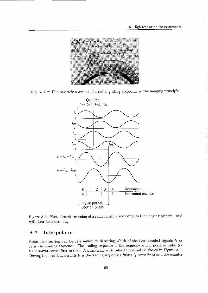
A. High resolution measurements
O
Figure A.2: Photoelectric scanning of a radial grating according to the imaging principle
Quadrant 1st 2nd 3rd 4th
I I I I I
o 1 2 3 4 increment 1 line count encoder
1 signal period 4 360" e!. phase
Figure A.3: Photoelectric scanning of a radial grating according to the imaging principle and with four-field scanning
A.2 Interpolator
Rotation direction can be determined by detecting which of the two encoded signals 11 or 12 is the leading sequence. The leading sequence is the sequence which positive pulse (or sinus-wave) comes first in time. A pulse train with velocity reversals is shown in Figure A.4. During the first four periods 11 is the leading sequence (Pulses 11 come first) and the counter
60
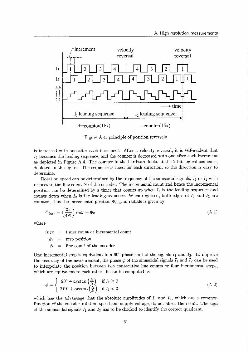
A. High resolution measurements
- time i I, leading sequence I, leading sequence i
4 L I - _,_ D'
velocity !IT rincrement reversal
velocity reversal
1 0 ~~~ o o-
I ++counter( 16x) --counter( 15x)
Figure A.4: principle of position reversals
is increased with one after each increment. After a velocity reversal, it is self-evident that 12 becomes the leading sequence, and the counter is decreased with one after each increment as depicted in Figure A.4. The counter in the hardware looks at the 2-bit logical sequence, depicted in the figure. The sequence is fixed for each direction, so the direction is easy to determine.
Rotation speed can be determined by the frequency of the sinusoidal signals, 11 or 12 with respect to the line count N of the encoder. The incremental count and hence the incremental position can be determined by a timer that counts up when 11 is the leading sequence and counts down when 12 is the leading sequence. When digitised, both edges of 11 and 12 are counted, thus the incremental position @incr in radials is given by
aincr = (-&) incr + where
incr = timer count or incremental count
@O = zero position N = line count of the encoder
One incremental step is equivalent to a 90" phase shift of the signals 11 and 12. To improve the accuracy of the measurement, the phase 4 of the sinusoidal signals 11 and I2 can be used to interpolate the position between two consecutive line counts or four incremental steps, which are equivalent to each other. It can be computed as
90" + arctan (2) if 11 2 O
4 = { 270" + arctan (2) if 11 < O
which has the advantage that the absolute amplitudes of 11 and 12, which are a common function of the encoder rotation speed and supply voltage, do not affect the result. The sign of the sinusoidal signals 11 and 12 has to be checked to identify the correct quadrant.
61
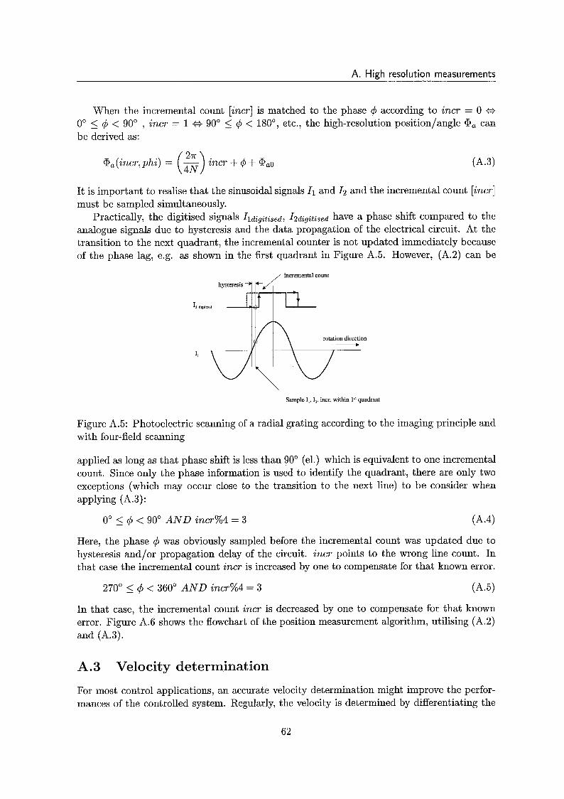
A. High resolution measurements
When the incremental count [incr] is matched to the phase q5 according to incr = O ($
O" 5 4 < 90" , incr = 1 e 90" 5 q5 < lso", etc., the high-resolution position/angle @a can be derived as:
@a (incr, phi) = (&) incr + 4 + ~~0
It is important to realise that the sinusoidal signals 11 and 1 2 and the incremental count [incr] must be sampied simuitaneousiy.
Practically, the digitised signals l l d i g i t i s e d , 12d ig i t i s ed have a phase shift compared to the analogue signals due to hysteresis and the data propagation of the electrical circuit. At the transition to the next quadrant, the incremental counter is not updated immediately because of the phase lag, e.g. as shown in the first quadrant in Figure A.5. However, (A.2) can be
incremental count
I, digbfllrd
rotation direction
Sample I,, 12, incr, within 1" quadrant
Figure A.5: Photoelectric scanning of a radial grating according to the imaging principle and with four-field scanning
applied as long as that phase shift is less than 90" (el.) which is equivalent to one incremental count. Since only the phase information is used to identify the quadrant, there are only two exceptions (which may occur close to the transition to the next line) to be consider when applying (A.3):
O" 5 q5 < 90" A N D incr%4 = 3 (A.4)
Here, the phase q5 was obviously sampled before the incremental count was updated due to hysteresis and/or propagation delay of the circuit. incr points to the wrong line count. In that case the incremental count incr is increased by one to compensate for that known error.
270" 5 q5 < 360" A N D incr%4 = 3 (A.5)
In that case, the incremental count incr is decreased by one to compensate for that known error. Figure A.6 shows the flowchart of the position measurement algorithm, utilising (A.2) and (A.3).
A.3 Velocity determination
For most control applications, an accurate velocity determination might improve the perfor- mances of the controlled system. Regularly, the velocity is determined by differentiating the
62
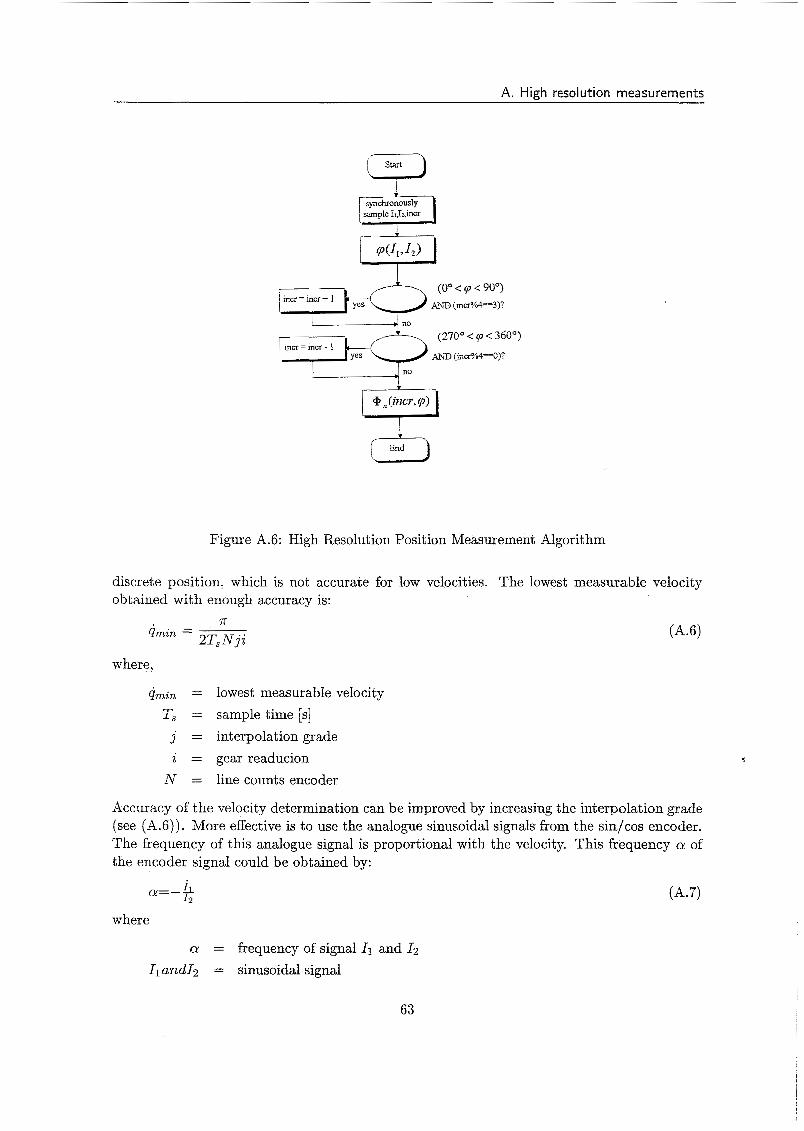
A. High resolution measurements
(270' < 9 < 360O) incr = incr - 1
m~ (ii~r0/04==0)7
Figure A.6: High Resolution Position Measurement Algorithm
discrete position, which is not accurate for low velocities. The lowest measurable velocity obtained with enough accuracy is:
7 1
where,
Qmin = lowest measurable velocity r n I s = sample time [SI
j = interpolation grade i = gear readucion N = line counts encoder
Accuracy of the velocity determination can be improved by increasing the interpolation grade (see (A.6)). More effective is to use the analogue sinusoidal signals hom the sin/cos encoder. The frequency of this analogue signal is proportional with the velocity. This frequency Q of the encoder signal could be obtained by:
Q=-Ll I2
where
Q = frequency of signal 11 and 12 Ilandl2 = sinusoidal signal
63

A. High resolution measurements
Then, the velocity becomes
q=LL N
Research must be done how to build an electrical circuit that performs (A.?). With this electrical circuit, the position can be obtained analoguously.
Performing (A.7) in discrete time the maximum sampling time must be taken into account:
1 r-7 I ,(maz) = ___ 8(q)Ni
In (A.9) the assumption has been made that 8 samples per period are necessary to rebuild a sinusoidal signal uniquely in discrete time, (factor 8 in equation) A.9. Performing experiments with the robot and using (A.9), the sample time becomes 3.125 10-6, with a maximum velocity of 1 [rad/s], a gear reduction of 8 and an encoder with 5000 line counts per revolution. This sample frequency is very high, so it is worthwhile to research the possibilities to obtain the velocity with analogue technologies.
A.4 Conclusion
With use of a sin/cos encoder a much higher resolution can be achieved than with a TTL encoder with identical counts. Using sin/cos encoders some hardware is required to interpolate the signal with the necessary accuracy. Application of the sin/cos encoders interfaced to an interpolator have the advantage of either a higher position resolution or reduced sensor cost, since sin/cos encoders requires less counts as equivalent TTL-encoder to achieve the same resolut ion.
64

Appendix B
Configuration of the pendulum system
1. Sliding contacts. Connects the signals of the encoder (no. 13) with the fixed world
2. Fixed hollow shaft for wires encoder no. 13. Shaft is ixed with the world beneath the motor with no. 10.
3. Hollow shaft from reduction gearbox, rotating.
4. Planetary reduction gearbox (i=8.192) with hollow shaft.
5. Asynchronous or induction motor.
6. Connectors induction machine
7. Inductive gauge, for cog wheel.
8. Assembling plate.
9. Electronics for inductive gauge (no. 7).
10. Fixation hollow shat no. 2.
11. Frame.
12. Arm.
13. Encoder pendulum.
14. Pendulum (not assembled during experiments).
15. Cogwheel.
16. High resolution sin/cos encoder.
17. Hollow motor shaft
18. Wires from pendulum encoder.
65
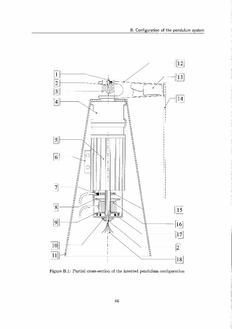
B. Configuration of the pendulum svstem
M M I I I
lsi
U
U
Figure B. 1: Partial cross-section of the inverted pendulum configuration
66

Appendix C
Data acquisition of the pendulum system
1. Computer.
2. DSPACE, data acquisition unit. Reads en sends analogue and digital signals.
3. Power electronics. The rotor is supplied by a “Pulse With modulation” source inverter, reading input signal (item 11) and send three phase signals with a fundamental frequency to the motor of the pendulum.
4. Pendulum machine configuration.
5 . Three phase wires.
6. Motor encoder signal 50 teeth per revolution.
7. Encoder pendulum.
8. High resolution encoder for arm.
9. Possibility to read signals motor encoder or high-resolution encoder.
10. Interpolator. Interpolates the sinusoidal input and send TTL signals to the DSPACE. Degree of interpolation can be changed with dip-switches.
11. Analogue signal from DSPACE to power-electronics.
67

C. Data acquisition of the pendulum system
Figure C.l: data acqüisition of the inverted pendulum configcration
68