MODELLING THE BACKGROUND NOISE IN A MASSSPECTROMETER FOR DENOISING APPLICATIONS

MENTOR: ANTHONY KEARSLEY, NATIONAL INSTITUTE OFSTANDARDS AND TECHNOLOGY,

RICHARD BARNARD, LOUISIANA STATE UNIVERSITY,YUTHEEKA GADHYAN, UNIVERSITY OF HOUSTON,

YOUZUO LIN, ARIZONA STATE UNIVERSITY,LIN TONG, IOWA STATE UNIVERSITY,

JIAPING WANG, RUTGERS UNIVERSITY, ANDGUANGJIN ZHONG, MICHIGAN TECHNOLOGICAL UNIVERSITY

1. Introduction

We look at the problem of denoising a spectrum arising from a massspectrometer. In order to achieve this, we develop a model which de-scribes the chemical noise using a stochastic differential equation. Thismodel then allows us to use a localized image denoising algorithm toachieve improved denoising. It also is able to predict instrument errorand generate additional spectra for simulation purposes. We concludewith some numerical results.

2. Mass Spectrometry

Mass spectrometry is a useful tool in analyzing the chemical makeupof a variety of substances in various fields. For instance, it is usefulin the field of combinatorial chemistry, a tool for drug discovery [13].It is also finding uses in the growing field of microbial forensics [15],an area of increased recent interest [14]. The mass spectrometer inour cases is a matrix-assisted laser desorption/ionization time-of-flight(MALDI-TOF) mass spectrometer which will give us a measurementof the time of flight of ions that have been charged by a laser. Theresult is a spectrum which associates intensity with time of flight.

In this paper we consider the problem of denoising data for a givenspectrum obtained through MALDI-TOF mass spectrometry performedon a polystyrene sample. A typical spectrum will consist of 25,000 to100,000 data pairs. One such spectrum can be seen in Figure 2. Closeup, the data is clearly highly noisy. In order to analyze the spectrum,peak identification is crucial, as described in [2]. However without

1

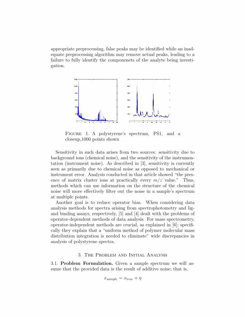
appropriate preprocessing, false peaks may be identified while an inad-equate preprocessing algorithm may remove actual peaks, leading to afailure to fully identify the componenets of the analyte being investi-gation.

Figure 1. A polystyrene’s spectrum, PS1, and acloseup,1000 points shown

Sensitivity in such data arises from two sources: sensitivity due tobackground ions (chemical noise), and the sensitivity of the instrumen-tation (instrument noise). As described in [3], sensitivity is currentlyseen as primarily due to chemical noise as opposed to mechanical orinstrument error. Analysis conducted in that article showed “the pres-ence of matrix cluster ions at practically every m/z value.” Thus,methods which can use information on the structure of the chemicalnoise will more effectively filter out the noise in a sample’s spectrumat multiple points.

Another goal is to reduce operator bias. When considering dataanalysis methods for spectra arising from spectrophotometry and lig-and binding assays, respectively, [5] and [4] dealt with the problems ofoperator-dependent methods of data analysis. For mass spectrometry,operator-independent methods are crucial, as explained in [6]; specifi-cally they explain that a “uniform method of polymer molecular massdistribution integration is needed to eliminate” wide discrepancies inanalysis of polystyrene spectra.

3. The Problem and Initial Analysis

3.1. Problem Formulation. Given a sample spectrum we will as-sume that the provided data is the result of additive noise; that is,

xsample = xtrue + η

Figure 2. PS1 and its background after differencing twice

where xsample is the observed data in a given spectrum arising froma sampled polystyrene, xtrue is the true signal, and η is a noise term.We are also provided xbkgd which is a spectrum obtained by using thespectrometer with out a sample loaded. The problem we shall addressin this paper, then, is to denoise xsample using, in part, informationobtained from the background spectrum xbkgd. We will assume in thispaper that the noise will be greater when a sample is loaded [1] Underthese assumptions, we can filter out a significant portion of the chemicalnoise from the data, xobs, to obtain a better approximation of xtrue.

When developing an algorithm to denoise the data we will have toconsider several constraints. Our algorithm will need to avoid using anya priori knowledge on the noise beyond the above general hypotheses.In light of this and the desire to reduce operator bias, we must alsoavoid algorithms that involve parameter selections that depend on anoperatorwhen analysing xobs; this will enable us to avoid introducingoperator bias. Finally, we wish to ensure that when we denoise our datawe are under-denoising our signal. This is a significant requirement, asoverly smoothing our data will remove peaks in xtrue, the locations ofwhich are crucial for analysis of the spectrum.

3.2. An Initial Attempt at Modelling. With the above in mind, wefirst attempt to model the chemical noise using an ARIMA model. Thebenefits of such a model, if appropriate, is the relative ease in develop-ing the model, along with an extensive theory having been developed.We first will check stationarity in our background spectrum. If we findstationarity, then we can establish two properties of the chemical noise.First, we will know that its mean and variance are not time-dependent.Secondly, we will see that covariance between points will be a functionof how far apart they are in the time only.

Figure 3. PS1, PS3 and their backgrounds after differ-encing twice

Figure 4. ACF and PACF of twice differenced ps1 noise

In both Figure 2 and Figure 3, we see that the second order dif-ferencing does not reveal stationarity. However, we notice that thetwice differenced PS1 data has an auto-correlation pattern indicatingthe possibility of seasonality, as seen in Figure 4. Putting aside sta-tionarity considerations for the moment, we attempt to fit the noise tothe genereal seasonal ARIMA model

(1) (1−p∑i=1

φiBi)(1−

P∑j=1

ΦjBjs)Wt = (1−

q∑i=1

θiBi)(1−

Q∑j=1

ΘjBjs)et

where BsWt = Wt−s, B1 = B and et is white noise. We will take forour modelling p = P = q = Q = 1 and s = 2. We will need to take(1− B)2Xt = W − t to model the twice differenced data with this fit.We solved for the parameters φ,Φ, θ,Θ using the standard function inR.

Figure 5. Residuals, ACF of residuals, and p-values ofLjung box for Seasonal ARIMA model of PS1 noise

The diagnostic plots shown in Figure 5 reveal that though this sea-sonal model removes 1-lag auto-correlation successfully, its residual isstill severely correlated in other lags. Therefore, time series may notbe an appropriate tool here to model our data behavior. This prelim-inary analysis leads us to consider more intricate models to describethe chemical noise.

4. Stochastic Differential Equation with time dependentcoefficients

Preliminary analysis of the background using time series establishednon stationarity and time dependent behaviour of the background. Wemodel the dynamics of the background using a general time dependentStochastic Differential Equation.

dXt = (a0(t) + a1(t)Xt)dt+ b0(t)XtdWt

Xt is the background at time t and {Wt} is a Wiener Process, Wt−Ws ∼N(0, t− s), s < t

The drift and the diffusion terms in the above equation are both linearfunctions of Xt. We assume a0(t)anda1(t) to be smooth functions of t.

In the next two sections we estimate the parameters and compute theexpected value and variance of Xt at each t. We use the local varianceof Xt to segment the noisy spectrum and then denoise over each seg-ment separately. The variance over each segment of Xt is computed asthe average of the variance over that segment.

4.1. Estimating Parameters. We are given the background data{Xti} at discrete points

t0 < t1 < · · · < tN

with ti+1 − ti = ∆.

Using Euler-Maruyama discretization:

∆Xti = (a0(ti) + a1(ti)Xti)∆ + b0(ti)Xti∆Wti

Assuming sufficient smoothness of the coefficients we use the followingapproximation at any point t0

(2) ai(t) = ai(t0), i = 0, 1

for t in a small neighborhood of t0. Let h denote the size of the neigh-borhood. The h is called the bandwidth or window size. We estimateai(t) using a locally weighted least squares approximation. We use thefollowing one sided Epanechnikov Kernel:

(3) Kh(u) =3

4h(1− u2) u ∈ (−1, 0)

At each point ti denoting aj(ti) by aj(i) we solve the following qua-dratic minimization problem:

(4) mina,b

N∑j=1

(Xtj+1

−Xtj

∆− a0(i)− a1(i)Xtj )

2Kh(ti − tjh

)

Kh 6= 0 on (-1,0) and 0 everywhere else, h window of data pointsconsidered for regression. We solve the first order conditions to obtainthe following expressions for aj(i), j = 0, 1 where aj(i), j = 0, 1 are thelocal estimators of aj(i), j = 0, 1.

a0(i) =

∑Nj=1 YtjKi −∆a1(i)XtjKh(tj − ti)

∆∑N

j=1Kh(tj − ti)(5)

a1(i) =

∑Kh(tj − ti)

∑YjXjKh(tj − ti)−

∑YjKh(tj − ti)

∑XjKh(tj − ti)

∆(∑Kh(tj − ti)

∑KhX2

j − (∑KhXj)2)

(6)

where Yj = Xj+1 −Xj.

With these estimates for aj(ti) j = 0, 1 i = 1, 2, . . . , N we have :

∆Xti − (a0(ti) + a1(ti)Xti)∆ ≈ b0(ti)Xti∆Wti

Using the notation:

(7)∆Xti − (a0(ti) + a1(ti)Xti)∆

∆= Ei

we have from the properties of a Weiner Process, given information upto time ti

b0(ti)Xti∆Wti ∼ N(0, b0(i)2X2

ti∆)

Therefore the conditional log-likelihood of Ei given Xti is approxi-

mately :

− log b0(i)2X2

ti

2− E2

i

2b0(i)2X2ti

In order to estimate b0(i) we approximate it locally by a constant :

(8) b0(t) = b0(t0),

in a neighborhood of size h. We maximize the log-likelihood of Ei givendata in a window of size h. Again we use the Epanechnikov one sidedkernel to assign weights to the data points according to their distancefrom the point where b0 is being estimated. We maximize the followingapproximate local likelihood function :

(9) maxb−1

2

N∑j=1

Kh(tj − tih

)(log(b2X2ti

) +E2i

b2X2ti

)

Again solving the first order condition for b we have :

b0(ti) =

∑Nj=1Kh(tj − ti)E2

i |Xti |−2∑Nj=1Kh(tj − ti)

With the estimates for aj(i) and b0(i) the dynamics of the backgroundis given by the following discrete approximation of the SDE :

∆Xti = (a0(ti) + a1(ti)Xti)∆ + b0(ti)Xti∆Wti

4.2. Computing the Mean and Variance. Next we compute themean and variance of Xt at every point t. Going back to the continuousSDE for Xt and observing

E

∫ t

t0

b0(s)XsdWs = 0

we have

E[Xt] = E[Xt0 ] +

∫ t

t0

(a0(s) + a1(s)E[Xs])ds

Differentiating both sides with respect to t and denoting E[Xt] by ftwe have the following differential equation:

(10) f ′t = a0(t) + a1(t)ft

Using a first order forward Euler finite difference scheme with time step∆ we have :

fti+1= fti + (a0(ti) + a1(ti)fti)∆

ft0 = Xt0

Next we compute the conditional variance of Xti+1given information

up to time ti. From the Euler discretization of Xt we have given Xti

V ar(Xti+1) = (b0(ti)Xti)

2∆

Once we have characterized the noise, we turn to denoising the massspectrum through data preprocessing.

5. Data Preprocessing

The setup of our problem is posed in a canonical inverse model, i.e.,by given the measured sample signal, we are going to find the corre-sponding original clean signal. A regularization technique is often usedwhen either the inverse model is ill-posed or to take into considera-tion of some kind of prior knowledge of the noise. Two of the morecommon regularization techniques are Tikhonov Regularization [7] andTotal Variation (TV) Regularization [8], where Tikhonov Regulariza-tion is formulated as,

(11) minx

{f(x) = ||Ax− b||22 + λ||Lx||22

},

and TV Regularization is given by,

(12) minx

{f(x) = ||Ax− b||22 + λ||∇x||1

}.

The choice of the technique depends on the characteristics of theproblem and our expectations for the solution. TV is well known forits ability to preserve the edges of the image / signal, while Tikhonv iseasy to implement from the computational point of view, and there isa much more well-established theory for Tikhonov than TV. In light ofthis, we first start with Tikhonov Regularization, then briefly discussthe possibility of using TV Regularization in our future work.

5.1. Inverse Model. As we mentioned previously, Tikhonov Regu-larization (11) will be used in our denoising model. In order to utilizethe model, two parameters need to be set before solving for the model,one is the regularization matrix, which is posed as L in (11), and theother one is the regularization parameter, λ in (11). The matrix of Lcan be the identity, derivative or Laplacian operator which promotesdifferent smoothness across the whole signal; in our numerical test, weused the derivative operator since we tended to see that by using theother two options the reconstructed signal will either be oversmoothedor undersmoothed. When it comes to selecting the other parameter λ,implementing the process becomes more difficult since there is no suchstraightforward way to pick the appropriate value in the sense of signalto noise ratio (SNR), and the value of λ is very influential on the SNRof the reconstructed signal.

5.2. Parameter Selection. Among the existing parameter selectionmethods, we can put them all into two categories: those assuming thatsome a priori, knowledge of the noise, such as variance, is given suchas, UPRE and discrepancy method [11], and those that do not, suchas L-Curve [9], and GCV [10]. In our case, since we can model thebackground noise–that is, we will be able to know the local variance ofthe noise–the first type of the parameter estimation methods is appro-priate. Specifically we will use UPRE.

UPRE method is short for the Unbiased Predictive Risk Estimator,which is an unbiased estimator of the mean squared error of predictiveerror Pλ of,

(13)1

n||Pλ||2 =

1

n||xλ − xtrue||2,

where xλ is the computed solution, and xtrue is the original clean signal.Since we do not know about xtrue, Vogel in [11] derives the unbiasedestimator for (13) in the Tikhonov case. (For the TV case, please refer

to Lin and Wohlberg’s work in [12]) The UPRE formula is given by,

U(λ) = E(1

n||Pλ||2)

=1

n||rλ||2 +

2σ2

ntrace(Aλ)− σ2,

where rλ = xλ−(xsample+η), Aλ = (I+λI)−1, σ2 is the variance of thenoise and n is the size of the problem. Based on the above definition,the optimal λ is defined to be,

(14) λopt = minλ{U(λ)} .

5.3. Segmentation. Domain decomposition (DD), or segmentation asmentioned in our report, is an technique that people use a lot in deal-ing with differential equations that having significant different regionsin terms of some kind of characteristics. In our problem, one thingis clear: the noise cannot be easily modeled uniformly over the wholeregion, but we can split the region into several segments and find outthe noise characteristics from each one of them, then use them to es-timate the corresponding optimal parameters λ on all the segments.Our numerical results shows the strength of using DD by comparingwith the results by using one global λ.

6. Numerical Tests

7. Simulating the Spectrum

We fit an SDE to the spectrum in the same manner as the back-ground and obtain the corresponding coefficients. The graph belowshows that the simulated data is very close to the actual spectrum.This is significant as generating a spectrum experimentally is very ex-pensive, taking as long as one day. The SDE model can be used toaccurately generate spectra. The graph below compares a simulatedspectrum to an actual spectrum.

Figure 6. Simulated and Actual Spectra

7.1. Picking peaks through variance. The location of genuine peaksin the spectrum can be found by comparing the variance or the errorof regression in the background to the spectrum. Low variance regionsin spectrum corresponding to high variance in the background can bethought of as fictitious peaks while high variance regions correspondingto low variance in background can be considered to be genuine peaks.Regions where the variance is high both in the background and thespectrum could be a genuine or fictitious peak. This is illustrated inFigure 7 below. The first set of figures correspond to data points be-tween 0 to 500 while the second corresponds to data between 10000 to11000 points.

7.2. Detecting Instrument Error. The diffusion coefficients b0(t)that appear in the SDE for the spectrum capture the error in thespectrometer. The quality of the instrument decays slowly at first andthen deteriorates rapidly . The plot of bti with respect to time capturesthis expected behavior of the instrument. Figure 8 illustrates the decayin the instrument.

7.3. Generating Synthetic Data. In order to test our algorithm’sdenoising qualities, we first must create spectra for testing. We useda Savitzky-Golay smoothing process twice on PS1 and PS3, to obtaina smooth spectrum. This was performed with the matlab commandsvgolayfit, using a 2nd order polynomial regression with framesize 45.

Figure 7. Two portions of the spectrum: the first 500points of the spectrum and points 10000-11000

We selected this method, as opposed to a standard adjacent averagingprocess, in order to preserve the general structure and locations oflocal maxima and minima. The resulting smooth data,smoothedPS1and smoothedPS3, is shown in

Figure 8. Predicting Instrument error

Figure 9. Smoothed Version of PS1

Figure 10. Smoothed Version of PS3

We now add noise to smoothedPS1 and smoothedPS3 that will mimicthe original data. For our purposes, we will generate three test spec-tra, test1, test2, from smoothedPS1 and test3 smoothedPS3. In eachexample, the noise term, η wll be of the form

(15) η = α · xtrue · ζ.

For test1 and test3 we segment the spectrum at the 10,000th datapoint, and for test2 we segment at the 3,000th and 11,000th segments.The term ζ for test1 is Cauchy on each segment, albeit with differentvariances for each segment. For test2 we set ζ to be a Beta termmultiplied with a Bernoulli term on each segment, again with differingmeans and variances on each segment. Finally, for test3, ζ is Gaussianon each segment, with different means and variances.

We choose these noise terms to approximate the structure of PS1and PS2:

Though the noised data sets are close to the original polystyrenespectra, their fundamental structure are different. We can see thisfrom differencing in 13 and 15 or in terms of auto-correlation factor(ACF) in 14 and 16. Thus, though the synthetic data are noisy spectrasharing with a passing resemblance to the actual polystyrene spectra,we can confirm that the background does not resemble a noisy signaloriginating from one of these simpler sources.

7.4. Denoising Algorithm. Our denoising procedure is as follows.We first use our stochastic differential equation model for the noisybackground spectrum to determine the pointwise variances and means

Figure 11. Histogram and density plots of, from left toright, PS1, test1, and test3

Figure 12. Histogram and density plots of PS3 and test2

of the noise. We then partition our spectrum for denoising into seg-ments whose noise behaves in some uniform fashion. In order to dothis, we take a rolling integral of the pointwise variance over framesof size 200 points and when we detect a 10% change, we begin a newsegment. In order to maintain a minimum image size for our denoisingprocess, we will require a minimum segment length of 1000 data points.After having segmented the data, we then move to denoising the data.

As stated in 5.2, we need to select an appropriate regularizationparameter λ in order to denoise our data in an optimal fashion. Thiswill be performed on each segment individually. As stated above, we

Figure 13. Comparison of PS1 with test1,test2 aftertwo differences

Figure 14. Comparison of ACF of PS1,test1,test2

will use UPRE in order find such a λ; as this algorithm assumes auniform variance in our noise, we use the mean of the variance oneach segment as a way to characterise the noise for our parameterestimation. Having found our parameter, we shift the signal by thepointwise mean of the noise and solve 11 on each segment with thatsegment’s regularization parameter. The shift is due to the requirement

Figure 15. Comparison of PS3 with test3 after two differences

Figure 16. Comparison of ACf of PS3,test3

in Tikhonov regularization to have zero-mean noise. This will result inour denoised spectrum.

We performed this algorithm on our test spectra. We took the noisethat was added to be the background spectrum. In 7.4 we comparethe Signal to Noise Ratio (SNR) for the synthetic data after denoisingwithout segmentation (simply using the variance of the entire spec-trum) and by using the above described algorithm. As can be seen,the segmentation delivers a significant improvement in the denoising.The segmentation algorithm is able to better balance data fidelity andsmoothing as the variance changes greatly over the entirety of the spec-trum.

Table 1. SNR of Synthetic Data Before Smoothing,Without Segmentation, and With Segmentation

Before Global Tikhonov Segmented Tikhonov

test1 11.4795 12.4840 19.2765test2 13.0861 17.9658 19.8942test3 9.7683 11.4497 15.3959

8. Conclusions and Future Work

We looked at the problem of denoising spectra arising from massspectrometers. Using background spectra, we modeled the chemi-cal noise that arises in mass spectrometry. We first discarded stan-dard time-series models, such as the ARIMA model, as the noise ishighly nonstationary, even after several differencings. We then lookedto model the chemical noise using a stochastic differential equation.This model uses only instrument specific-parameters to characterizethe noise accurately. We are able to use this model to find the lo-cal mean and variance of the chemical noise and simulate additionalspectra for future analysis. We then used a locally tuned Tikhonov de-noising algorithm to improve denoising over a globally tuned Tikhonovalgorithm.

Our segmentation algorithm is currently the only portion of our de-noising process involving user-input. We have not investigated theeffect of tuning the tolerance in shifts in the tolerance, nor the effecton the minimum segment length. Finally, our segmentation algorithmresults in disjoint segments. There may be an improvement in thedenoising process if we allow for overlap in our segments and then per-form a mortaring procedure. Naturally, the mean of the local varianceon each segment may not be the optimal way to characterize the vari-ance on the entire segment, which is a required input for the UPREalgorithm. We would like investigate other criteria for changes in thebehavior of the noise that would lead to an automatic segmentationalgorithm. We have also not fully investigated other methods for de-noising the data, such as TV regularization. However, we expect asimilar improvement as TV regularization benefits from a better senseof the noise using the SDE model.

References

[1] Wallace, W. E., Guttman, C. M., Flynn, K. M., Kearsley, A. J., ‘Numericaloptimization of matrix-assisted laser desorption/ionization time-of-flight massspectrometry: Application to synthetic polymer molecular mass distribution

measurement Analytica Chimica Acta Volume: 604 Issue: 1 Special Issue:Pages: 62-68 NOV 26 2007

[2] Wallace, W. E., Kearsley, A. J., Guttman, C. M., ‘An operator-independentapproach to mass spectral peak identification and integration Analytical Chem-istry. Volume: 76 Issue: 9 Pages: 2446-2452. MAY 1 2004

[3] Kruthinsky,A. N. and Chait, B. T., ’On the Nature of the Chemical Noise inMALDI Mass Spectra’ Journal of the American Society for Mass Spectrometry.Volume: 13 Issue: 2 Pages: 129-134, 2002

[4] Little, J. A. ‘Comparison of curve fitting models for ligand binding assays ’Chromatographia Volume: 59 Pages: S177-S181 Supplement: Suppl. SS Pub-lished: 2004

[5] Santana, D. W. E. A., Sepulveda, M. P., Barbeira, P. J. S. ’Spectrophotometricdetermination of the ASTM color of diesel oil’ Fuel Volume: 86 Issue: 5-6Pages: 911-914 MAR-APR 2007

[6] Guttman, C. M., Wetzel, S. J., Blair, W. M., Fanconi, B. M., Girard, J.E., Goldschmidt, R. J., Wallace, W. E., VanderHart, D. L. ’NIST-SponsoredInterlaboratory Comparison of Polystyrene Molecular Mass Distribution Ob-tained by Matrix-Assisted Laser Desorption/Ionization Time-of-Flight MassSpectrometry: Statistical Analysis’ Analytical Chemistry Volume: 73 Issue: 6Pages: 152-1262 MAR 1 2001

[7] A. N. Tikhonov, ’Regularization of Incorrectly Posed Problems’ Soviet MathDokl. Volume: 4 Pages: 1624 - 1627, 1963

[8] L. Rudin and S. Osher and E. Fatemi, ’Nonlinear Total Variation Based NoiseRemoval’ Physica D, 60, Pages: 256 - 268, 1992

[9] P. C. Hansen and D. P. O’Leary, ’The Use of the L-curve in the Regularizationof Discrete Ill-Posed Problem’ SIAM Journal on Scientific Computing. Volume:14 Pages: 1487 - 1503, 1993

[10] G. H. Golub and M. T. Heath and G. Wahba, ’Generalized cross-validation asa method for choosing a good ridge parameter’, Technometrics. Volume: 21Pages: 215 - 223, 1979

[11] C. R. Vogel, ’Computational Methods for Inverse Problems’ SIAM, 2002[12] Y. Lin and B. Wohlberg, ’Application of the UPRE Method to Optimal Param-

eter Selection for Large Scale Regularization Problems’ 2008 IEEE SouthwestSymposium on Image Analysis and Interpretation Pages: 89 - 92, 2008

[13] Kassel, D.B. ’Combinatorial chemistry and mass spectrometry in the 21st cen-tury drug discovery laboratory’ Chemical Reviews Volume: 101 Issue: 2 Pages:255-267 FEB 2001

[14] Dance, A. ’Anthrax case ignites new forensics field’ Nature Volume: 451 Page:813 AUG 2008

[15] Jarman, K. H., Kreuzer-Martin, H. W., Wunschel, D. S., Valentine, N. B.,Cliff, J. B., Petersen, C. E., Colburn, H. A., Wahl, K. L. ’Bayesian-IntegratedMicrobial Forensics’ Applied and Environmental Microbiology Volume: 74, Is-sue: 11 Pages: 3573-3582 JUNE 2008

[16] Epanechnikov, V.A. ’Nonparametric estimation of a multidimensional proba-bility density,’ Theor. Prob. Appl. Volume: 13, Pages: 153-158 1969

[17] Fan, J., Jiang, J., Zhang, C., Zhou, Z. ’Time-dependent Diffusion Models forTerm Structure Dynamics’ Statist. Sinica Volume: 13 Issue: 4, Pages: 965-992.2003

[18] Kloeden, P. E., Platen, E. ’Numerical Solution of Stochastic Differential Equa-tions’ Springer, 1999

[19] Protter, E. ’Stochastic Integration and Differential Equations, Second Edition,Springer, 2005