1

Modeling Time Series of Counts

Richard A. DavisColorado State University

William DunsmuirUniversity of New South Wales

Sarah StreettNational Center for Atmospheric Research

(Other collaborators: Richard Tweedie, Ying Wang)

2

Outline

+ Introduction

Examples

+ Linear regression model

+ Parameter-driven models

Poisson regression with serial dependence

Theory for GLM estimates

+ Observation-driven models

Properties

Existence and uniqueness of stationary distributions

Model for stock prices (number of trades and price activity)

Estimation and asymptotic theory for MLE

Application to asthma data

3

Example: Daily Asthma Presentations (1990:1993)

Year 1990

••••••••••

•••••

•••••••••••••••••

•••••

•

••••••

••••••••••••

••••

•••••••••••

••••••••

•••••••••

•••

•••••

•

••••••

•••••

••

•

•••••••••••••••••••••

••

••••••

•••••

•••••••

••••

•

••••••••••••

•

•••••••••

••

•

•••

•

••••••

•••••••••

•

••••••••••••••

•••••••

••••••••••

••••••••••

••••••••••••

••••••

•••••

•••••••••••••••••

••••••

••••

•••••••••••

••••••••••••

•

•••••••••••••

•••••

••••••••••••

••••••••

••••••

••••

06

14

Jan Feb Mar Apr May Jun Jul Aug Sep Oct Nov Dec

Year 1991

••••••

••••••••••••

•••••••••

••••••••

•••••

•••••••

••••••

••••••

••••••

•••••••••

••

•••

••••••

•

•••••••

•

••••••

••••••••

••••••••••••••

•••••

•••••

•

•

•

•••

•••••••••

••••••••

••••••••

••••••••••••

•

•••••••

••••

••••••

•••••••••••

•••••

•••••••

•

••••••••••••

••••

••••••••••

•••••••••••••••••••••••••••

••••••••

•••••

•••••

••••••••••

•••••••

•••••••••••••

•••••

•••••••••••••••••••••••

••••••••••

•••••••••

06

14

Jan Feb Mar Apr May Jun Jul Aug Sep Oct Nov Dec

Year 1992

•

•••••••••

••••••••••••••••••••

••••••••

•••••••••••

•••••••

••

••

••••••••••

••

•

••

•••••

•••••

••••••

•••••••

•••

••••

••••••••••

•••

•••••••••

•••••••••

••••••

••

•

••

•

•

••

•

•••••••

•

•••••••

••••

•

•••••

••••••

•••••••••

••••••••••••

••••••

•••••••••

••••

••••••••

•••

••••••••

••••••••

•••••••••••••

•••••

••••••

••••••••••

••••••••

•••••••

•••••••••

•••••••••

•

•••••••

•••••••••

••••••••••••

••••••••

•••••

•••••••0

614

Jan Feb Mar Apr May Jun Jul Aug Sep Oct Nov Dec

Year 1993

••••••••••••

••••••••

•••••

•••••

•••••••••••

•••

••••

••

••••

••••

•

•

•••••••

•

•••••••••••

••

•••••••••

••••

••

••

••••••••

•••••••••

••••••••

•••••••••••

•

•••••••••••

••••

••••••

••

••••••

••

•••••

•••••••••••

•••••••••

•••••••

••••

••••••••••••

•••••••

•••••

••••••••

••••••

•••••••

•••••

•••••••

•••••

•••••

•••••

•••••••••

•

••••••••••••••••••••

••••

••••

•••••••

•••••••••••••••••••••

••••

•••••••••

••••••••••••0

614

Jan Feb Mar Apr May Jun Jul Aug Sep Oct Nov Dec

4

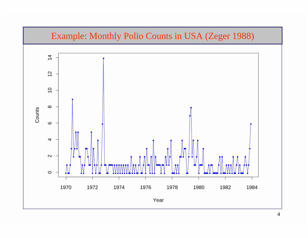
Example: Monthly Polio Counts in USA (Zeger 1988)

Year

Cou

nts

1970 1972 1974 1976 1978 1980 1982 1984

02

46

810

1214

•••••

•

•

••

•

•

•

••

••••

•••••

•

•

•

•••

•

•••

•

•

••••••••

••••••••••••••••

•

••••••••

••••

•

•

•••

•

•

•

•

•••••

••••

••

•

••

•

•••••••

••

•

•••

••

•

••

•

•

•••

•

••••

•

•••••••••••••

••

•

•

•••••••••

•

••••

•••••

•••••

•

•

5

Notation and Setup

Count data: Y1, . . . , Yn

Regression (explanatory) variable: xt

Model: Distribution of the Yt given xt and a stochastic process νt are indep

Poisson distributed with mean

µt = exp(xtT ββββ + νt).

The distribution of the stochastic process νt may depend on a vector of

parameters γγγγ.

Note: νt = 0 corresponds to standard Poisson regression model.

Primary objective: Inference about β.β.β.β.

6

Example: Polio (cont)

Regression function:

xtT=(1, t´/1000, cos(2πt´/12), sin(2πt´/12), cos(2πt´/6), sin(2πt´/6))

where t´=(t-73).

Summary of various models fits to Polio data:

Study Trend(β) SE(β) t-ratioGLM Estimate -4.80 1.40 -3.43Zeger (1988) -4.35 2.68 -1.62Chan and Ledolter (1995) -4.62 1.38 -3.35Kuk&Chen (1996) MCNR -3.79 2.95 -1.28Jorgensen et al (1995) -1.64 .018 -91.1Fahrmeir and Tutz (1994) -3.33 2.00 -1.67

7

Suppose Yt follows the linear model with time series errors given byYt = xt

T ββββ + Wt ,

where Wt is a stationary (ARMA) time series.

• Estimate ββββ by ordinary least squares (OLS).

• OLS estimate has same asymptotic efficiency as MLE.

• Asymptotic covariance matrix of depends on ARMA parameters.

• Identify and estimate ARMA parameters using the estimated residuals,Wt = Yt - xt

T

• Re-estimate ββββ

and ARMA parameters using full MLE.

Linear Regression Model-A Review

ββββOLS

ββββOLS

8

GLM Estimation

Model: Yt | νt , xt ∼ PP((exp(xtT ββββ

++++ νt )).

GLM log-likelihood:

(Likelihood ignores presence of the latent process.)

Assumptions on regressors:

−+−=) ∏∑∑===

n

tt

n

t

n

tYYel

111

!log( ββββββββ ββββ Ttt

x xTt

),()(

),(

1 1

1,

1

1,

βΩ→−γµµ=Ω

βΩ→µ=Ω

∑∑

∑

=ε

=

−

=

−

II

n

ts

n

stnII

I

n

ttnI

tsn

n

Tst

Ttt

xx

xx

9

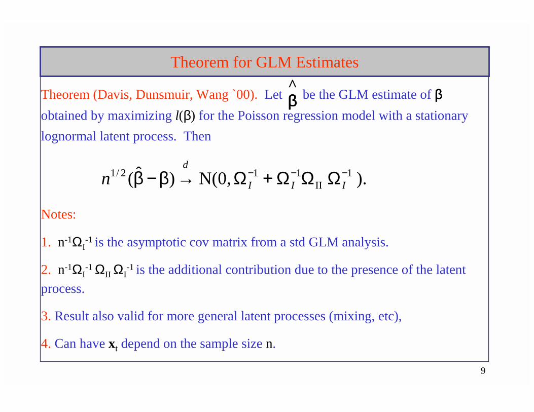
Theorem for GLM Estimates

Theorem (Davis, Dunsmuir, Wang `00). Let be the GLM estimate of ββββobtained by maximizing l(β) for the Poisson regression model with a stationarylognormal latent process. Then

Notes:

1. n-1ΩI-1 is the asymptotic cov matrix from a std GLM analysis.

2. n-1ΩI-1 ΩIIΩI

-1 is the additional contribution due to the presence of the latentprocess.

3. Result also valid for more general latent processes (mixing, etc),

4. Can have xt depend on the sample size n.

^ββββ

). N(0, )ˆ( 1II

112/1 −−− ΩΩΩ+Ω→β−β III

dn

10

When does CLT Apply?

Conditions on the regressors hold for:

1. Trend functions.xnt = f(t/n)

where f is a continuous function on [0,1]. In this case,

Remark. xnt = (1, t/n) corresponds to linear regression and works. However xt = (1, t) does not produce consistent estimates say if the true slope is negative.

.)()()()(

,)()(

)(21

01 1

1

)(1

01

1

∑∫∑∑

∫∑

εβ

=ε

=

−

β

=

−

γ→−γµµ

→µ

h

tn

ts

n

st

tn

tt

hdtetttsn

dtettn

ffxx

ffxx

T

T

fTTst

fTTtt

11

When does CLT apply? (cont)

2. Harmonic functions to specify annual or weekly effects, e.g.,

xt = cos(2πt/7)

3. Stationary process. (e.g. seasonally adjusted temperature series.)

12

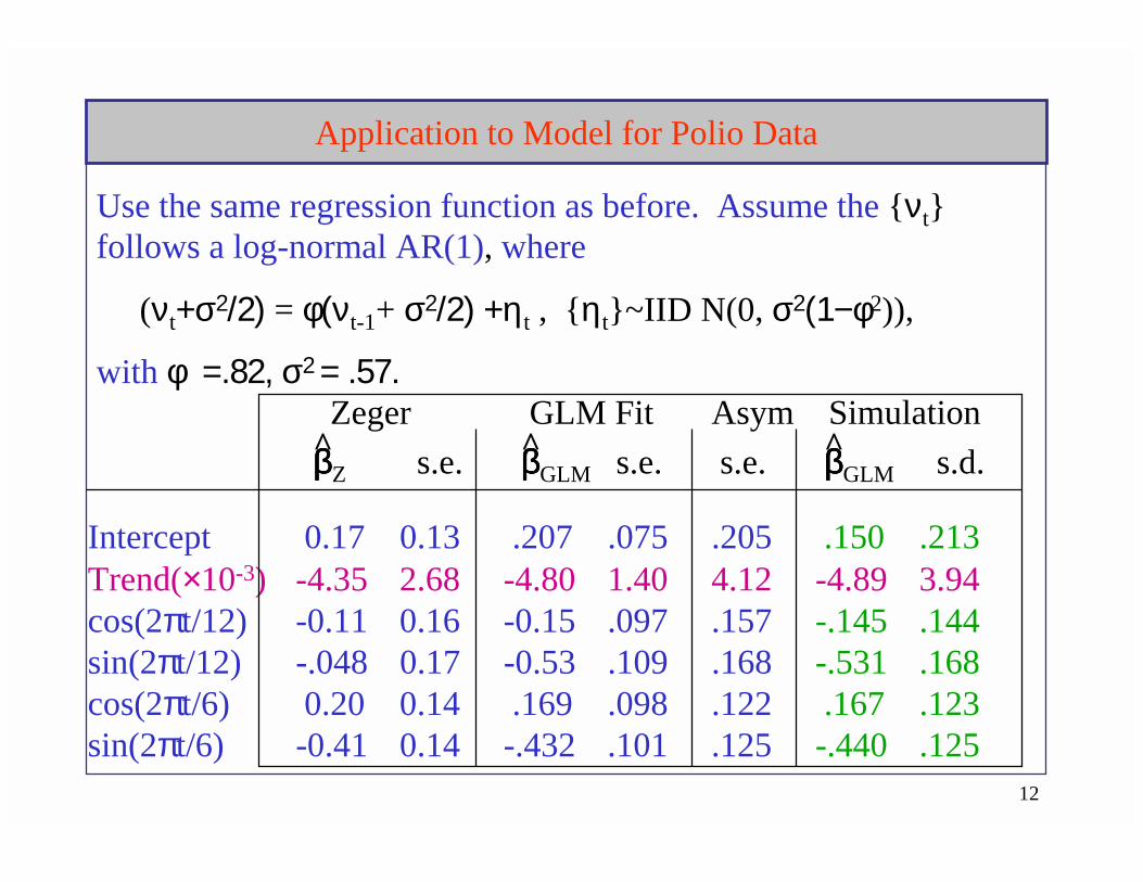
Application to Model for Polio Data

Use the same regression function as before. Assume the νtfollows a log-normal AR(1), where

(νt+σ2/2) = φ(νt-1+ σ2/2) +ηt , ηt~IID N(0, σ2(1−φ2)),

with φ =.82, σ2 = .57.Zeger GLM Fit Asym Simulation

Intercept 0.17 0.13 .207 .075 .205 .150 .213Trend(×10-3) -4.35 2.68 -4.80 1.40 4.12 -4.89 3.94cos(2πt/12) -0.11 0.16 -0.15 .097 .157 -.145 .144sin(2πt/12) -.048 0.17 -0.53 .109 .168 -.531 .168cos(2πt/6) 0.20 0.14 .169 .098 .122 .167 .123sin(2πt/6) -0.41 0.14 -.432 .101 .125 -.440 .125

ββββZ s.e. ββββGLM s.e. s.e. ββββGLM s.d.

13

Polio Data With Estimated Regression Function

Year

Cou

nts

1970 1972 1974 1976 1978 1980 1982 1984

02

46

810

1214

•••••

•

•

••

•

•

•

••

••••

•••••

•

•

•

•••

•

•••

•

•

••••••••

••••••••••••••••

•

••••••••

••••

•

•

•••

•

•

•

•

•••••

••••

••

•

••

•

•••••••

••

•

•••

••

•

••

•

•

•••

•

••••

•

•••••••••••••

••

•

•

•••••••••

•

••••

•••••

•••••

•

•

14

Model for the Mean Function µt

Parameter-driven specification: (Assume Yt | µt is Poisson(µt ))

log µt = xtTββββ + νt ,

where νt is a stationary Gaussian process. e.g. (AR(1) process)

(νt + σ2/2) = φ(νt-1 + σ2/2) + εt , εt ~IID N(0, σ2(1-φ2)).

Advantages:• properties of model (ergodicity and mixing) easy to derive.• interpretability of regression parameters

E(Yt ) = exp(xtT ββββ )Εexp(νt) = exp(xt

Tββββ ), if Εexp(νt) = 1.Disadvantages:

• estimation is difficult-likelihood function not easily calculated (MCEM, importance sampling, estimating eqns).

• model building can be laborious• prediction is hard.

15

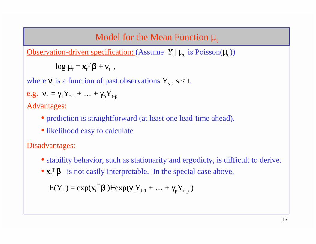
Model for the Mean Function µt

Observation-driven specification: (Assume Yt | µt is Poisson(µt ))

log µt = xtTββββ + νt ,

where νt is a function of past observations Ys , s < t. e.g. νt = γ1Yt-1 + … + γpYt-p

Advantages:• prediction is straightforward (at least one lead-time ahead).• likelihood easy to calculate

Disadvantages:

• stability behavior, such as stationarity and ergodicty, is difficult to derive.• xt

T ββββ

is not easily interpretable. In the special case above,

E(Yt ) = exp(xtTββββ )Εexp(γ1Yt-1 + … + γpYt-p )

16

New Observation Driven Model

Two components in the specification of νt (see also Shephard (1994)).

1. Uncorrelated (martingale difference sequence)

For λ > 0, define

(Specification of λ will be described later.)

2. Form a linear process driven by the MGD sequence et

where

Since the conditional mean µt is based on the whole past, the model is no longer Markov. Nevertheless, this specification could lead to stationary solutions, although the stability theory appears difficult.

λµµ tttte /)Y( −=

.

,xlog

1

Tt

iti

it

tt

e −

∞

=∑=

+=

ψν

νβµ

17

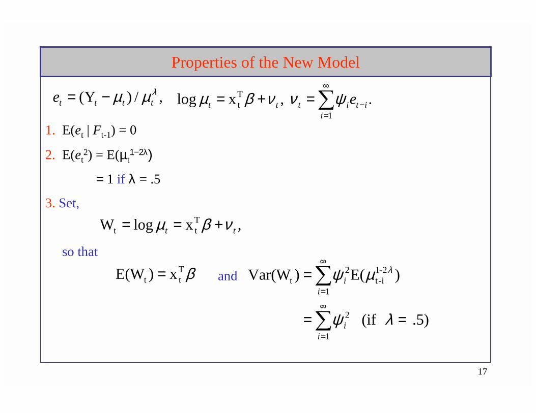
Properties of the New Model

1. E(et | Ft-1) = 0

2. E(et2) = E(µt

1−2λ)

= 1 if λ = .5

3. Set,

so that

and

,/)Y( λµµ tttte −= . ,xlog1

Tt it

iittt e −

∞

=∑=+= ψννβµ

,xlogW Ttt tt νβµ +==

βTtt x)E(W =

.5) (if

)E()Var(W

1

2

2-1i-t

1

2t

==

=

∑

∑

∞

=

∞

=

λψ

µψ λ

ii

ii

18

Properties continued

4.

It follows that Wt has properties similar to the latent process specification:

which, by using the results for the latent process case and assuming the linear process part is nearly Gaussian, we obtain

It follows that the intercept term can be adjusted in order for E(µt) to be interpretable as exp(xt

Tβ).

,

)()(

2/x

2/)(x

x

1

2Tt

Tt

Tt

∑+

+

+

∞

=

−

=

≈

∑=

ii

t

i itit

e

e

eEeEVar

eW

ψβ

νβ

ψβ

)E()W,Cov(W 2-1i-t

1htt

λµψψ hii

i +

∞

=+ ∑=

iti

ie −

∞

=∑+=

1

Ttt xW ψβ

19

Existence and uniquess of a stationary distr in the simple case.Consider the simplest form of the model with λ = 1, given by

Theorem: The Markov process Wt has a unique stationary distribution.

Idea of proof:

• State space is [β−γ, ∞) (if γ>0 ) and (- ∞, β−γ] (if γ< 0 ).

• Satisfies Doeblin’s condition:

There exists a prob measure ν such for some m > 1, ε > 0, and δ >0,

ν(A) > ε implies Pm(x,A) ≥ δ.

• Chain is strongly aperiodic.

• It follows that the chain Wt is uniformly ergodic (Thm 16.0.2 (iv) inMeyn and Tweedie (1993))

.)Y(W 1-t1-t -WW1t eet −+= −γβ

20

Existence of Stationary Distr in Case .5 ≤ λ <1.Consider the process

Propostion: The Markov process Wt has at least one stationary distribution.

Idea of proof:

• Wt is weak Feller.

• Wt is bounded in probability on average, i.e., for each x, the sequenceis tight.

• There exists at least one stationary distribution (Thm 12.0.1 in M&T)

Lemma: If a MC Xt is weak Feller and P(x, •), x∈ X is tight, then Xt is bounded in probability on average and hence has a stationary distribution.

Note: For our case, we can show tightness of P(x, •), x∈ X using a Markov style inequality.

.)Y(W 1-t1-t W-W1t

λγβ eet −+= −

,...,2,1 ),,(1

1∑ =

− =⋅k

ii kxPk

21

Uniqueness of Stationary Distr in Case .5 ≤ λ <1?Theorem (M&T `93): If the Markov process Xt is an e-chain which is bounded in probability on average, then there exists a unique stationary distribution if and only if there exists a reachable point x*.

For the process , we have

• Wt is bounded in probability uniformly over the state space.

• Wt has a reachable point x* that is a zero of the equation0 = x* + γ exp(1-λ) x*

• e-chain?

Reachable point: x* is a reachable point if for every open set O containing x*,

for all x.

e-chain: For every continuous f with compact support, the sequence of functions Pnf , n =1,… is equicontinuous, on compact sets.

1-t1-t W-W1t )Y(W λ− −γ+β= eet

∑∞

=>

10),(

nn OxP

22

Modeling Framework for Stock Prices (Rydberg & Shephard)Consider the model of a price of an asset at time t given by

where

• N(t) is the number of trades up to time t

• Zi is the price change of the ith transaction.

Then for a fixed time period ∆,

denotes the rate of return on the investment during the tth time interval and

denotes the number of trades in [t ∆, (t+1) ∆).

,)0((t))(

1∑=

+=tN

iiZpp

, )())1((:))1((

1)(∑

−∆+

+∆=

=∆−−∆+=tN

tNiit Ztptpp

)())1((: ∆−−∆+= tNtNNt

23

The Bin Model for the Number of TradesBin(p,q) model: The distribution of the number of trades Nt in [t ∆, (t+1) ∆), conditional on information up to time t ∆− is Poisson with mean

Proposition: For the Bin(1,1) model,

there exists a unique stationary solution.

Idea of proof:

• λt is an e-chain.

• λt is bounded in probability on average.

• Possesses a reachable point ( x∗ = α/(1−γ) )

.1,0 ,0 ,N11

t <δγ≤≥αλδ+γ+α=λ ∑∑=

−=

− jj

q

jjtj

p

jjtj

,N 1-t1t δλ+γ+α=λ −t

24

A Simple GLARMA Model for Price Activity (R&S)Model for price change: The price change Zi of the ith transaction has the following components:

• At activity 0,1

• Dt direction -1,1• St size 1, 2, 3, . . .

Rydberg and Shephard consider a model for these components. An autologistic model is used for At .

Simple GLARMA model for price activity: At is a Bernoulli rv representing a price change at the tth transaction. Assume At given Ft-1 is Bernoulli(pt), i.e.,

P(At = 1 | Ft-1) = pt = 1- P(At = 0 | Ft-1),

where

.)1(

and )1( 1-t1-t

1-t1t pp

pAUe

ep ttU

U

t

t

−−=

+= −

σ

σ

25

Existence of Stationary for the Simple GLARMA Model .Consider the process

where At-1 is Bernoulli with parameter

Propostion: The Markov process Ut has a unique stationary distribution.

Idea of proof:

• Ut is an e-chain.

• Ut is bounded in probability on uniformly over the state space

• Possesses a reachable point ( x∗ is soln to x+eσx/2=0 )

, )1( 1-t1-t

1-t1

pppAU t

t −−= −

.)1( 1t

−+= tt UU eep σσ

26

Estimation for Poisson Observation Driven Model

Let δ = ( βT, γT)T be the parameter vector for the model (γ corresponds to the parameters in the linear process part).

Log-likelihood:

where

First and second derivatives of the likelihood can easily be computed recursively and Newton-Raphson methods are then implementable. For example,

and the term can be computed recursively.

),)(WY()L( )(Wtt

1

t δδδ en

t−=∑

=

.)(x)(W1

tt iti

i e −

∞

=∑+= δψβδ

δδ

δδ δ

∂∂−=

∂∂

∑=

)(W)Y()L( t)(Wt

1

ten

t

δδ ∂∂ /)(Wt

.

,xlog

1

Tt

iti

it

tt

e −

∞

=∑ψ=ν

ν+β=µ

Model: Yt | µt is Poisson(µt )

27

Asymptotic Results for MLE

Define the array of random variables by

Properties of ηnt:

•ηnt is a martingale difference sequence.

•

•

Using a MG central limit theorem, it “follows” that

where

.)(W)(Y t)(Wt

2/1 t

δδη δ

∂∂−= − ennt

).()|(1

1 δηη VFE Pn

tt

Tntnt →∑

=−

.0)|)|(|(1

1 →>∑=

−P

n

ttnt

Tntnt FIE εηηη

),,0()ˆ( 12/1 −→− VNn Dδδ

).()(1lim1

)( δδδ Ttt

n

t

W

nWWe

nV t ∂∂= ∑

=∞→

28

Simulation Results

Model 1:

Parameter Mean SD SD(from like)β0 = 1.50 1.499 0.0263 0.0265γ = 0.25 0.249 0.0403 0.0408β0 = 1.50 1.499 0.0366 0.0364γ = 0.75 0.750 0.0218 0.0218β0 = 3.00 3.000 0.0125 0.0125γ = 0.25 0.249 0.0431 0.0430β0 = 3.00 3.000 0.0175 0.0174γ = 0.75 0.750 0.0270 0.0271

Model 2:

β0 = 1.00 1.000 0.0286 0.0284β1 = 0.50 0.500 0.0035 0.0034 γ = 0.25 0.248 0.0420 0.0426β0 = 1.50 0.998 0.0795 0.0805β1 = -.15 -.150 0.0171 0.0173γ = 0.25 0.247 0.0337 0.0339

5000nreps 500,n ,)Y(W 1-t1-t -WW10t ==−γ+β= − eet

5000nreps 500,n ,)Y(500/W 1-t1-t -WW110t ==−γ+β+β= − eet t

29

Application to Sydney Asthma Count DataData: Y1, . . . , Y1461 daily asthma presentations in a Campbelltown hospital.

Preliminary analysis identified.

• no upward or downward trend

• a triple peaked annual cycle modelled by pairs of the formcos(2πkt/365), sin(2πkt/365), k=1,2,3,4.

• day of the week effect modelled by separate indicatorvariables for Sundays and Monday (increase in admittance on these days compared to Tues-Sat).

• Of the meteorological variables (max/min temp, humidity)and pollution variables (ozone, NO, NO2), only humidity at lags of 12-20 days appears to have an association.

30

Model for Asthma DataTrend function.

xtT=(1, St, Mt, cos(2πt/365), sin(2πt/365), cos(4πt/365), sin(4πt/365),

cos(6πt/365), sin(6πt/365), cos(8πt/365), sin(8πt/365))

(No humidity used in this model.)

Model for ν t.

νt = (1/φ(B) − 1) et , where φ(B) is the AR(10) with autoregressivepolynomial

φ(B) = 1 − φ1B − φ3B3 − φ7B7 −φ10B10.

Note: the νt can be computed recursively.

31

Results for Asthma Data

Term Est SEIntercept 0.533 0.029Sunday effect 0.240 0.054Monday effect 0.249 0.054cos(2πt/365) -0.162 0.036sin(2πt/365) 0.362 0.035cos(4πt/365) -0.067 0.036sin(4πt/365) 0.023 0.034cos(6πt/365) -0.083 0.035sin(6πt/365) 0.009 0.035 cos(8πt/365) -0.157 0.034sin(8πt/365) -0.062 0.034

φ1 0.053 0.024φ3 0.061 0.024φ7 0.078 0.024 φ10 0.053 0.024

32

Asthma Data w/ Deterministic Part of Mean Fcn

Year

Cou

nts

1990 1991 1992 1993 1994

02

46

810

1214

33

Asthma Data: Deterministic Part + AR in Pearson Resid

Year

Cou

nts

1990 1991 1992 1993 1994

12

34

5

••••••••

•••••

••

•••••

••

•••••

•••••••

••

••

••••

•

•

•••

•

•

•

•••••

••

•••••

•

•

•••

•

•

••

•••••

••

•••••••

•••••

•••••••

•

•

•

•

•••••

•••••

••

••••

•••••••••

•

••••

•

••

•••••

••

•••

•

••

•

•••

•

•

••

••••

•••

••••••

•

•••••

•••

••••

•

•

••

•

•

•

•

•

•••••

•

•

•••••

••••••••••••••

•

••••••

••

•••••

••

•••••••

••••••••••••••

••••••••••••

••••••••••••••

••

••••••••••••

•••••••

••

•••••

•••••••

••

•

••••

•••

••••••••••

•

••

•••••

••

•••••

••

••••••••••••••••••••••••••

••

•••••

•••••••

•••••••

••

•••••••

•••

•

•

•••••••

•

•••••

•••

••••

•

••

•••••

••

•••••

•

••

•

•

••

••

••

•

••

•

•••

•••

•••••••

••

•••

••

•

•

•••••

••

•••••

••

•••

•

••

•

•••••••

••••

•

•••••••

••

•••••

••

•••••

••

•••••

•••

••••••

•••••

••

•••••

•••••

•

•••

•••••

••••••••

•

••

•••

••

•••••

•••••••••

•••••

•••••••••••••••••••••

••••••••••••••

••

•••••••••••••••••••

••••••••••••••

••

•••••••

•••••

••

•••••••••••••••••••••••••••••••••

••••

•••

••

••••••••••••

••

•••••

••

•••••

•••

•••••

•

•••

••

•

••••••

•

••••

••

•

•

••••

•

•

•

•

•

••

••

•

•

••••••

••••••

•

•

••

••

••

•

••••

••

•••••

••

•••••

•••

••••

••

•••••

•

•

•••••

•

•

•

•

•

•

•

•

•

•••••

•

•

••

•••

••

•••••

••

••••

•

••

••

•

••

••

•••••

••

•••••••

•••••

••

•••••

••

•••••

••

•••••

••

••••••

•

•••••

••

•••••

••••••••••••••••

•••••

••

•••••

•••••••••

•••••

•••••••••••

••••••••••

•••••••

••

•

•

•

•

•

•••

•••••••••••••

•••••

••••••••••••••

••

••••••••••••••

•••••

•••••••••

•••••

•••••••

••

•

••••

••

•••

•

•

•

•

•

•

•

••

•

•

•

•

••

•

•

•

•

••••

••

•

••••

••

••••

•

••

•••••

••

•••••

••

•••

•

•

••

•

••••

•••••••••

•

••••••

•

••••

••

•••••

••

•••

••

••

•••

•

••

•

•••••

••

•••••

•••••••

••

•••••••

••••••••••••

••

•••••

•

••••••

•••••••

••

•••••

••••••••••

•

•

••••

•••••

••

•••••

••

•••••

•••••••

••

•••••••

••••••••••••••

•••••

•••••••••

•••••••

•••••

•••••••

••••••••••••••

•

••••••

••••••••••••••••••••

det. partdet. part + AR

34

Summary RemarksThe observation model for the Poisson counts proposed here is

1. Easily interpretable on the linear predictor scale and on the scale of the mean µt with the regression parameters directly interpretable as the amount by which the mean of the count process at time t will change for a unit change in the regressor variable.

2. An approximately unbiased plot of the µt can be generated by

3. Is easy to predict with.

4. Provides a mechanism for adjusting the inference about the regression parameter β for a form of serial dependence.

5. Generalizes to ARMA type lag structure.

6. Estimation (approx MLE) is easy to carry out.

.)ˆ5.ˆexp(ˆ1

2∑∞

=

−=i

itt W ψµ