Patick T. Brandt is a Visiting Lecturer in Political Science, Indiana University, WoodburnHall 210, Bloomington, IN 47405 (pbrandt@indiana.edu). John T. Williams is Professorof Political Science, Indiana University, Woodburn Hall 210, Bloomington, IN 47405(jotwilli@indiana.edu). Benjamin O. Fordham is Assistant Professor of Political Science,University at Albany, State University of New York, 135 Western Avenue, Albany, NY12222 (fordham@cnsvax.albany.edu). Brian Pollins is Associate Professor of PoliticalScience, The Ohio State University, Columbus, OH 43201 (pollins.1@osu.edu).

An earlier version of this work was presented at the 1998 Summer Meetings of the Po-litical Methodology Group, University of California, San Diego. Williams’s research wassupported by National Science Foundation grant SBR-9422645. Pollins’s research wassupported by the Mershon Center of the Ohio State University. All GAUSS code used forthis analysis is available with documentation at http://www.polsci.indiana.edu/jotwilli/home/default.htm. We wish to thank Chris Achen, Neal Beck, Michael Craw, John Free-man, Simon Jackman, Gary King, David LeBlang, Michael McGinnis, Walter Mebane,Stephanie Sillay, Jim Stimson, and Pravin Trivedi for their comments and suggestions.Standard disclaimers apply.

American Journal of Political Science, Vol. 44, No. 4, October 2000, Pp. 823–843

©2000 by the Midwest Political Science Association

S cholars use event-count models to analyze a wide variety of politicalscience data. For example, the large sets of data on cooperative andconflictual international events often use event-count models

(Huang, Kim, and Wu 1992; Sayrs 1992; Volgy and Imwalle 1995). Thesedata have also been analyzed using time-series methods, particularly whentransformed into indices of conflict and cooperation that consider the se-verity of each event and are no longer purely event counts (Goldstein 1991;Goldstein and Freeman 1990; Schneider, Widmer, and Ruloff 1993; Wardand Rajmaira 1992). Other event counts commonly analyzed in interna-tional relations include the number of wars (Benoit 1996; Mansfield 1992),militarized interstate disputes (Gowa 1998; Pollins 1996; Senese 1997), orother incidents of conflict and cooperation between states (Brophy-Baerman and Conybeare 1994; Eyerman and Hart 1996; Kinsella 1995;Kinsella and Tillema 1995; O’Brien 1996; Fordham 1998a, 1998b; Remmer1998). Scholars in American politics have also employed event-count mod-els for time-series data to analyze presidential activity (Brace and Hinckley1993), Federal Reserve decisions (Krause 1994), federal contract awards(Mayer 1995), executive orders (Krause and Cohen 1997), and SupremeCourt decisions (Caldeira and Zorn 1998). The same issues confront thesmaller number of comparativists using such data (Moore, Lindstrom, andO’Regan 1996).

Dynamic Modeling for PersistentEvent-Count Time Series

Patrick T. Brandt Indiana UniversityJohn T. Williams Indiana UniversityBenjamin O. Fordham University at Albany, State University of New YorkBrian Pollins Ohio State University

We present a method for estimating

event-count models when the data is

generated from a persistent time-

series process. A Kalman filter is

used to estimate a Poisson expo-

nentially weighted moving average

(PEWMA) model. The model is com-

pared to extant methods (Poisson

regression, negative binomial regres-

sion, and ARIMA models). Using

Monte Carlo experiments, we demon-

strate that the PEWMA provides sig-

nificant improvements in efficiency.

As an example, we present an analy-

sis of Pollins (1996) models of long

cycles in international relations.

. , . , . ,

We argue that a Poisson Exponentially WeightedMoving Average (PEWMA) model, based on Harvey andFernandes (1989), is a useful and tractable approach toevent-count time-series data that are persistent. Themodel assumes an underlying latent dynamic processthat is continuous, and this continuous process ismapped onto the observed discrete variable. Interpreta-tion of the dynamics is simple. The mean varies overtime, and a key parameter describes the amount of varia-tion over time in this mean. The impact of covariates iseven simpler to interpret. These have the same exponen-tial interpretation as do coefficients in the static Poissonregression model. We think that PEWMA will be a usefulcomplement to the tool kit of political scientists whoanalyze event-count data.

In the next section, we review a number of modelsfor persistent event-count time series and argue why thePEWMA is preferable for persistent event-count time se-ries. We then outline the PEWMA model for persistentevent counts.1 The model is based on structural time-se-ries models, as described in Harvey (1989). This struc-tural time-series (or state space) model for event-countdata is based on the representation similar to Harvey andFernandes (1989), and Harvey (1989). We then useMonte Carlo simulations to show that this dynamicevent-count model performs much better on efficiencygrounds than do Poisson and negative binomial models.Finally, we present an application of the PEWMA modelby revisiting Pollins’s (1996) analysis of long-cycle theo-ries in international relations in order to illustrate howour model can produce better inferences with persistentevent-count time series.

Approaches to Modeling Time-SeriesEvent-Count Data

The standard approach to modeling event-count data isto assume that the events are generated from a Poissondensity (King 1989a). The probability of observing thecount yt is given by a Poisson distribution with mean ar-rival rate λ:

Pr( | )

!y

e

yt

y

t

t

λ λλ=−

.

Using maximum-likelihood techniques, one can estimatethe Poisson mean parameter λ. When λ = exp(Xt β) theresult is a Poisson regression model. The Poisson regres-sion model assumes that events are independent so themean and variance of the model are equivalent: E[yt] =V[yt] = λ. When this assumption is violated, the varianceis usually larger than the mean and the events are consid-ered overdispersed. When the events are overdispersed,then alternative estimators have been proposed. Amongthese are the negative binomial and generalized eventcount (GEC) estimators (King 1989b).

The two main approaches to modeling time series ofevent counts in political science are to use GaussianARIMA models, or to include a lagged-dependent eventcount as a regressor in the mean function of a Poisson,negative binomial, or generalized event-count regressionmodel.

If yt is an event count, then ARIMA models assum-ing normally distributed errors are flawed in four ways.First, unless the values of the observations are very large,the event-count distribution may not be accurately ap-proximated by a normal distribution. Second, the modelmust produce predictions that are strictly positive to bevalid. If the mean number of events is small, then thepredictions may not be greater than zero—invalidatingthe model. Third, modeling event counts with a Gaussiandistribution leads to bias and inefficiency (King 1988).

Fourth, using differencing as is common in GaussianARIMA modelling for nonstationary event counts isproblematic. Using the first differences to deal with trendnonstationarity in count data is appealing because it isanalogous to the approach used for Gaussian time series.The main problem with modeling the first differences ofevent counts with a Gaussian model is the validity of thedistributional assumption. The difference of two inde-pendent Poisson variables has a known distribution.Derivations of the distribution of the difference of twoindependent Poisson random variables rely explicitly onthis independence assumption (Skellam 1946; Strackeeand van der Gon 1962). For time series of counts, this in-dependence assumption is clearly inappropriate. In gen-eral, we do not think it is true for time series of counts,and it is never true for trending series. Thus, the lack of awell-defined distribution for the difference of a series ofnonstationary event counts leads us to look for alterna-tive models that can describe the data generation process.

An alternative approach is to retain the assumptionof a Poisson or negative binomial distribution. Underthis approach possible dynamics in event-count data aremodelled with a lagged dependent variable in Poissonand negative binomial models. These models suffer fromtwo possible problems. First, they fail to represent ad-

1Elsewhere, Brandt and Williams (1998) develop a model formean-reverting or autoregressive event count time series. Thismodel, the Poisson autoregressive model of order p (PAR(p)) isbuilt using a method similar to the PEWMA. The PEWMA is in-tended for persistent or nonmean reverting data.

-

equately the dynamics in persistent time series becausethese models imply that the growth rate of the process isthe exponentiated coefficient on the lagged dependentvariable. Such a process may potentially generate time-series data, but not data that are dynamic. The laggedevent-count model is appropriate only for series with ex-ponential growth rates and no dynamics.2 This meansthat the lagged dependent Poisson and negative binomialmodels cannot be used to model stationary time series.Unless the time series of event counts has an exponentialdeterministic trend and no dynamics, this model haslimited applicability.

Time-Series Models for Event-Count Data

While political scientists have included lags in event-count models or used ARIMA models for time series ofevent counts, many other models have been proposed.The literature on time-series models for event-countdata contains a number of different methods for dealingwith dependence in event-count time series. In this sec-tion we review these alternative approaches and defendthe PEWMA as a very useful model.

In our view, there are three classes of time-seriesevent count models.3 The first class is integer-valuedARMA or Discrete Autoregressive Moving Average mod-els (DARMA). The second class is based on conditionalautoregressive or hidden Markov processes. These mod-els are based on a latent variable model. The final class ofmodels, which contains the PEWMA, is the state space ortime-varying parameter models.

Integer-valued / Discrete ARMA Models

The integer-valued AR (INAR), integer-valued ARMA(INARMA), or Discrete Autoregressive Moving Average(DARMA) models discussed by Alzaid and Al-Osh(1990), Du and Li (1991), and McKenzie (1988) are basedon probabilistic mixtures of different Poisson processes.

For example, the integer-valued AR(p) model is based ona marginal Poisson distribution. In each period, the ob-served number of events is defined by a binomial or mul-tinomial sampling procedure called “thinning.” The data-generating procedure for the event-count variable yt is ofthe form

y y tt i t i t

i

p

= + = ± ±−=∑α εo K

1

0 1 2, , , ,

where “ o” is the multinomial thinning operator, and εt isa nonnegative integer valued variable with fixed meanand known variance.4 This is a mixture of an event-count distribution (Poisson or negative binomial) and amultinomial distribution. Estimates of the autoregressivethinning parameters αi can be obtained by conditionalmaximum likelihood. To date, we are unaware of anygeneral implementation of this method. Squier (1996,1997) shows that including exogenous variables in thismodel is difficult and produces inconsistent and ineffi-cient estimates of the effects of exogenous variables. Inaddition, if covariates are included in this mixturemodel, it is not clear how to interpret the effects ofcovariates on the observed event-count time series.

Conditional Autoregressive/Hidden Markov Models

Conditional autoregressive models are based on assum-ing that the conditional distribution of the events yt , de-pends on a static mean function, and lagged-dependentvariables or serially correlated errors. For these models,the dynamics enter either as past yt s or through the errorprocess. Models in this class have been discussed byJackman (1998), Shephard (1995), Diggle, Liang, andZeger (1994), and Zeger (1988).

As an example, consider a static regression modelwhere the number of events yt depends on a set ofcovariates and a serially correlated error term that fol-lows an AR(1) process. Then the conditional mean of thenumber of events can be written as,

E yt t[ | ]ε = Xtβ + ut, ut= ρut–1 + εt ,

where εt is i.i.d.(0,σ2). This model can be estimatedby nonlinear least squares, or maximum-likelihood

2 The growth rate of this lagged Poisson regression model is givenby

ln(µt) – ln(µt – 1) = Xtδ – Xt – 1δ + ρzt – 1 – ρzt – 2.

Taking expectations gives

E[ln(µt) – ln(µt – 1)] = ρE[zt – 1 – zt – 2]

If ρ ≠ 0 and E[zt – 1 – zt – 2] ≠ 0, this model implies a nonzero growthrate for the conditional mean.

3See Davis, Dunsmuir, and Wang (1998a) and Cameron and Trivedi(1998, chapter 7) for alternative reviews of the literature.

4The thinning operation is defined as follows for the binomialcase: α o Xn is the sum of Xn–1 independent random Bernoullivariables, Yi

n−1 where Pr( ) Pr( )Y Yin

in− −= = − = =1 11 1 0 α . This

process gives rise to the same AR(p) coefficients and autocorre-lation function behavior as the standard Gaussian AR(p) model(Alzaid and Al-Osh, 1990).

. , . , . ,

methods depending on the assumptions about the dis-tribution of εt .

Alternatively, Zeger (1988), and Diggle, Liang, andZeger (1994) propose a latent-variable specification basedon:

E yt t[ | ]ε = exp(Xtβ)εt , Var yt t[ | ]ε = ut.

The estimator based on this model is identified ifE(εt) = 1 and Cov(εtεt+τ) = σ2ρε(τ). This specification ofthe latent-variable model can be estimated using a quasi-maximum-likelihood estimator that solves a set of gener-alized estimating equations (see Zeger 1988 for details).The standard Poisson regression model provides con-sistent estimates of the regression parameters for thismodel, even in the presence of a dynamic latent process(Davis, Dunsmuir, and Wang, 1998a). However, param-eter estimates will be inefficient when there is a signifi-cant amount of serial correlation in εt (Davis, Dunsmuir,and Wang 1998a, 17). Thus, inference based on thesemodels is open to the critique that the interpretation ofestimated parameters is imprecise.5

These examples with serially correlated errors are ac-tually a special case, since a model with AR errors can bewritten as a moving average model for the dependentvariable. The serial correlation in the errors imply that yt

has a moving average representation. An AR(1) errormodel suffers from the same limitations as a Gaussianmodel with AR(1) errors. Models with AR(1) error struc-tures may be appropriate in specific contexts, but theyare not general since they fit only a limited type of dy-namic processes. In addition, if lagged dependent countsare included in the model and there is still serial correla-tion in the error process, estimates will be inconsistent,just as in OLS models (Cameron and Trivedi, 1998: 227).Thus, inclusion of lagged counts, or serially correlated er-rors appears to be just as difficult in event count modelsas in standard Gaussian linear time-series models. Suchserial correlation can be analyzed using standardized re-

siduals and standard diagnostics for serial correlation(see Cameron and Trivedi, 1998: 228–229 for details).However, if data are nonstationary, models that assumestationarity will clearly be inappropriate. The next classof models relaxes this condition and allows for modelsthat can be either stationary with long memory or non-stationary.

State-space/Time-varying Models

The final class of models is based on a state-space repre-sentation specifying a measurement and transition equa-tion. For event counts, the measurement equation is anevent-count distribution, while the transition equationdescribes how the dynamics of the event count distribu-tion parameters evolve. The state-space approach is verygeneral because the models are specified in terms of thebasic structure of the time series: trends, cycles, and time-varying stochastic components. Examples of this ap-proach include Zeger and Qaqish (1988), Harvey (1989),Harvey and Fernandes (1989), West, Harrison, and Migon(1985), West and Harrison (1986, 1997), Chan andLedolter (1995), Kitagawa and Gersch (1996), Durbin andKoopman (1997, 2000), Davis, Dunsmuir, and Wang(1998a, 1998b), Jorgensen, Labouriau, and Lundbye-Christensen (1996), and Jorgensen et al. (1999).

As an example, Davis, Dunsmuir, and Wang (1998a,1998b) present a general state-space event count time-se-ries model. In their model, the conditional mean, or statevariable, for the event-count model incorporates bothautoregressive (AR) and moving average (MA) compo-nents. The conditional mean of the marginal Poisson dis-tributed event counts has the form,

E y Y X e X e

where ey

and ee

e

e

e

t t t t t t i t ii

tt t

t

i ti

i ii

p

i ii

q

| , , exp ,

,

.

− −=

∞

−=

∞ =

=

[ ] = = +

= −

=+

−

− =

( )( ) −

∑

∑∑∑

11

11

1

1

1

11 1

µ β τ

µµ

τγ

φ

γφ

Thus, event counts are Poisson distributed with

mean µt . The

τ i t iie −=

∞∑ 1 is the one-step-ahead predictor

of et based on an ARMA(p,q) process. While this modelis more general than what we present below, using higherorder dynamic terms in an ARMA filter primarily onlybenefits the forecasting ability of the model. The state-space models of Durbin and Koopman (1996, 1997) are

5Jackman (1998) proposes another “latent first order autoregres-sive model.” The latent mean for the event count yt has the form,

[ ] ( )

~ ( , ), , , , .

E y Xwhere v

and v N t T

t t t

t t t

t v

= += +

=−

exp β εε ρε

σ1

20 1 2 K

Note the similarity to Zeger’s GEE model. This model is identifiedby a distributional assumption on the AR(1) errors and corre-sponds to a Gaussian regression model with AR(1) errors. Since themodel’s parameters cannot be simultaneously estimated, Jackmanuses the EM-algorithm via a Markov Chain Monte Carlo methodto compute the maximum-likelihood estimates. This model and es-timation issues are also discussed in Davis, Dunsmuir, and Wang(1998a).

-

similar to these. Estimates can be obtained usingMarkov-Chain-Monte-Carlo methods or other numeri-cal solutions. While these models appear to offer an in-tuitive approach that is similar to existing ARIMA mod-els, the complexity of their estimation and high degree ofparameterization make inference difficult.

The state-space models of Chan and Ledolter (1995),Kitagawa and Gersch (1996), West, Harrison, and Migon(1985), and West and Harrison (1986, 1997) are based onBayesian dynamic linear models. While these are similarin spirit to the PEWMA we present, they are based onBayesian rather than classical assumptions. These modelstypically require the use of numerical methods such asMarkov-Chain-Monte-Carlo methods that are highly de-pendent on the specific model being estimated. More-over, the interpretation of exogenous covariates in thesemodels typically requires dynamic simulations. These re-quirements make implementing and interpreting thesemodels costly and could put them out of the reach ofmost political scientists. An alternative approach dis-cussed by Jorgensen, Labouriau, and Lundbye-Christen-sen (1996) and Jorgensen et al. (1999) is based on a clas-sical Kalman filter/smoother, but is more complex toestimate and interpret than our present approach.

There are several drawbacks to these alternatives.First, there exists little available software for easily imple-menting these models. Second, the interpretation of thesemodels is often complex and requires techniques beyondthose currently used to evaluate event-count data. Finally,several of the models produce poorly behaved or hard tointerpret estimates of the effects of exogenous covariates.This complicates inference and testing.

Our PEWMA state-space model suffers from noneof these problems and has several advantages. First, esti-mation is simple and fast. Estimation is done using a ver-sion of the Kalman filter rather than simulation meth-ods, which is robust and quick. For example, all of thePEWMA estimates in the six specifications in our ex-ample in Section Four take less than thirty seconds on astandard PC workstation using our software.6 Second,unlike some of the alternative time-series event countmodels, the interpretation of the effect of exogenousvariables does not require any new methods or simula-tion techniques. The standard Poisson regression modelis a special case of the PEWMA, and we can interpret thePEWMA coefficients just as we would any coefficient in astandard Poisson or negative binomial regression model.Finally, the dynamics in the PEWMA model are charac-

terized by a single parameter that takes on values be-tween zero and one. This allows for a simple and intuitiveevaluation of the model dynamics, unlike alternativeapproaches.

The Poisson Exponentially WeightedMoving Average Model

The Model

To model persistent event count time series, we use astructural time-series model. The intuition behind themodel is that the mean number of observed events to-day is a weighted sum of all the past events. This mean isdefined as a weighted average of the past events, plus arandom shock. The random shock is included to ac-count for unexpected changes in the mean number ofevents. The model discounts events in the distant pastmore heavily than those in the recent past. If the num-ber of events observed at each period in time is indepen-dent of past events, the model reduces to the standardPoisson regression.

Our model has two components. The first is a func-tion that describes how the observed number of eventsarises as a function of a mean number of events in thepast. It is called a measurement, or system equation in astructural time-series model. The measurement equationdescribes the process that generates the observed data.The second function describes how important pastevents are for predicting the number of events in the cur-rent period. It is called the state or transition equationand describes the dynamic transition process from eventsin the past to events in the present.

Once we have a model in state-space form, estimationof the model’s parameters proceeds using the Kalman fil-ter. Using a recursive algorithm, the Kalman filter com-putes the optimal estimates of the mean and other param-eters of the state equation of a state-space model at eachtime period using the information available up to thattime period. The Kalman filter works by finding the esti-mates of the model parameters in the state equation thatminimize the mean-squared error of the conditionalmean of the series (Harvey 1989, 104–105).

To identify and estimate the model we adopt the ap-proach of Harvey and Fernandes (1989). They employnatural conjugate densities to simplify the developmentof the model and numerical calculations.7 Using natural

6 This result is based on using our software code in Gauss 3.2 withMAXLIK 4.0.34 on a Pentium II workstation with 256 megabytesof memory.

7A conjugate density is a prior distribution that after being com-bined with a likelihood function yields a posterior distribution ofthe same form. A conjugate density is a natural conjugate density ifit is in the class of distributions with the same functional form as

. , . , . ,

conjugate densities to describe the unobserved param-eters of the model allows us to derive well-known closed-form distributions for the model parameters.

The model for time-series count data is based on astate-space form with a Poisson measurement equationand a gamma-distributed state equation. The model cap-tures the changes in the mean of a Poisson process attime t. We assume that the count at time t, denoted yt ,follows a Poisson distribution with a conditional mean attime t denoted µt , with explicit dependence on t. Thevariable µt is assumed to be gamma distributed, since thegamma is the conjugate distribution for the Poisson.With these assumptions, one can then derive the result-ing conditional forecast or predictive distribution for themean. In the estimation of the mean of µt , one needs toaccount for the history of the process up to and includingperiod t – 1. We denote this sequence of conditioningdata by the vector Yt – 1. This vector contains both past-observed values of counts yt, and any independent vari-ables Xt that have been observed up to and including pe-riod t – 1. The vector, Yt – 1 = (y0,y1, . . . , yt –1; X0, X1, . . .Xt – 1), is the full information set available at time t. In ad-dition, the model also contains a hyperparameter 0 < ω ≤1. This parameter allows the past observations to be dis-counted in making conditional forecasts of the mean offuture observations.8 Throughout the article, we use thenotation wt|t – 1 to represent the value of the random vari-able wt conditional on the observed-information set inthe previous t – 1 periods.

The Poisson-gamma exponentially weighted movingaverage model for count data (PEWMA) is built aroundthe following three assumptions that characterize themean and dynamics of the process:

(1) Measurement Equation: The observed counts attime t are drawn from a Poisson marginal distribution,

Pr( | )

!y

e

yt tty

t

t t

µ µ µ=

−. (1)

The parameter µt in this distribution is the unobservedmean-arrival rate for the count at time t. This unob-served mean µt is parameterized by the multiplicativeequation

µ µ δt t tX= −∗

1 exp( ), (2)

where δ is a K × 1 vector of coefficients, Xt a 1 × K vectorof explanatory variables (without a constant), and atime-varying component µ t−

∗1.9 As in Harvey and

Fernandes (1989), we assume that this separate time-varying level component µ t−

∗1 is a multiplicative factor.

This factor is estimated by the Kalman filter and accountsfor the observed counts prior to time t – 1. Thus, it is asmoothed mean of the previous observations.

(2) Transition Equation: The stochastic mechanismfor the transition in the series from time t – 1 to time t isa function of µt – 1 and µt . The dynamics of the mean aredescribed by a multiplicative transition equation withthe form,

µ µ ηtr

t te t Tt= =−1 1 2, , , , ,K (3)

where ηt is beta distributed, β(ωat – 1, (1 – ω)at – 1). Theparameter ω captures the discounting of the observa-tions in computing the mean and ηt and rt parameterizethe growth rate in period t. The beta-distributed variableηt captures the proportional stochastic shift in the meanfrom time t – 1 to time t. From the properties of the betadistribution, E[ηt ] = ω for all t. This means that the ex-pected stochastic shocks on average are equal to theweight of past event counts in the current event count.The parameter rt describes the growth in the series andinsures that µt > 0.10

(3) Conjugate Prior: The prior distribution for thetime varying component is a gamma distribution:

µ t t ta b−∗

− −1 1 1~ ( , )Γ . To identify the model in equations(1–3), we specify the gamma distribution as the conju-gate prior for the distribution of yt. The gamma density fis given by

the likelihood function. For example, if y is sampled from a Pois-son distribution with unknown mean λ, then the natural conju-gate prior that describes λ is the gamma distribution. If y issampled from a normal distribution with unknown mean µ andknown variance σ, then the natural conjugate prior is a normaldistribution (DeGroot 1970, 164,167).

8A hyperparameter is a parameter of a prior distribution not fixedat particular numerical values (Gelman et al. 1995, 36).

9Including a constant in the mean function is equivalent to speci-fying a deterministic trend.

10We caution readers who might use the Harvey and Fernandes(1989) model. Their transition equation provides an incorrectmodel of the stochastic process for the mean of event counts.Harvey and Fernandes adopted an alternative transition equationwith the form µt = µt – 1ηtω–1. However, Shephard (1994) citingNelson (1990) notes that if ω < 1, then µt converges to zero as t →∞. The reason for this is that the growth rate for the Harvey and

Fernandes’ transition equation can be approximated by

lnµµ

t

t−

1

= −ln( ) ln( )η ωt . By Jensen’s inequality, this quantity will be nega-tive on average. In their discussion of Harvey and Fernandes’model, Brockwell and Davis (1996) also note this problem, citingGrunwald, Hamza, and Hyndman (1997). We avoid this problemby adopting the transition equation suggested by Shephard’s(1994) work on local scale models. So far as we know, this is thefirst application of Shephard’s transition equation to a state-spacemodel for event count data.

-

f a b

e b

a

b a a

( ; , )( )

µ µµ=− −1

Γ, (4)

with a = at–1, b = bt–1, and µ µ= −∗t 1 . These values are

computed from the previous t – 1 observations, Yt –1.Using these assumptions, we can estimate a Kalman

filter using maximum-likelihood methods. The follow-ing sections describe the estimation and interpretation ofthe model.

Estimation

Estimation of the model requires a time-dependent se-ries of recursions for the conditional mean E Yt t[ | ]µ −1

and the posterior mean E Yt t[ | ]µ . These recursions definea Kalman filter for the Poisson measurement density andgamma-distributed transition equation. To compute thisfilter, we derive the recursions for the values of a, b, and µall evaluated at time t – 1 (the prior), at time t given t – 1(the conditional or predictive), and at time t (the poste-rior). These estimates are then used to compute the con-ditional or predictive distribution of the number ofevents in each time period. The predictive distributiondescribes the probability of observing events at time tconditional on all the events observed in each of the pre-vious t – 1 periods. It turns out that the predictive distri-bution for the PEWMA model is a negative binomial dis-tribution where the overdispersion in the observed datadepends on the amount of dependence between theevents in each time period. The details of these deriva-tions are included in Appendix A. Rather than focus onthe computations of these latent parameters of themodel, we turn to estimation and properties.

The predictive distribution combines the informa-tion in the measurement density and the transition equa-tion. That is, we observe events yt conditional on themean µt at time t. The value of µt then depends on theweighted average of the number of events observed inthe past.

The joint-predictive density, conditional on Yτ forobservations yτ+1, . . . , yT is:

Pr , , |

| | .

y y y Y

Y Y

T t tt

T

t t

Measurement

t t

Transitiont

T

ττ

τ

+ −= +

−∞

= +

( ) = ( )

= µ( ) ⋅ µ( )

∏

∫∏

1 11

101

K

1 24 34 1 24 34

Pr

Pr Pr(5)

The key to understanding this predictive distributionis the decomposition of the posterior probability

Pr( | )y Yt t −1 . Using the Kalman filter, we can condition

the observed data on the components of the predictivedistribution: the probability of the event (from a Poissondistribution) and the probability of the unobservedmean (from a gamma distribution). Note that these twocomponents correspond to the measurement and transi-tion equations.

Once we have the predictive distribution, we con-struct the log-likelihood function and estimate themodel using maximum-likelihood techniques. This ap-proach is identical to that used to derive the estimates ofa Gaussian ARIMA model.

Given the conditional probability density of y Yt t| −1,we can construct the log-likelihood function for the un-known hyperparameter and the parameters based on (5):

ln , | , , ,

!

ln ln

ln ln b exp

ln exp

t-1

L a b y X

y a y

a a X r

a y b X r

t t t t

t t tt

T

t t t t

t t t t t

ω δ

ω

ω ω ω δ

ω ω δ

τ

− −

−= +

− −

− −

( )= +( ) − ( )− ( ) + − −( )( )− +( ) + − −

∑

1 1

11

1 1

1 11

Γ

Γ

(( )( ).

(6)

Maximizing with respect to ω and δ provides an estimateof the hyperparameter and other parameters, respec-tively. Note that the computation of this likelihood re-quires an analytic solution for rt , which characterizes theper-period growth rate from period t – 1 to t. AppendixA presents the derivation of this quantity. Appendix Bdescribes the forecast function for the model.

Description of the PEWMA Process

The PEWMA model does not have a simple linear struc-ture. Thus, it is less than obvious how the dynamics ofthe PEWMA process evolve over time. In this section wecharacterize the evolution of a PEWMA time series byanalyzing the properties of the transition equation (3).Our characterization shows how the mean of the process,µt evolves over time.

The transition equation for the PEWMA impliesthat the mean evolves according to a random-walk pro-cess. Recall that the transition equation is written

µ = µµ( ) − µ( ) = + ( )

−

−

tr

t t

t t t t

e

so r

t1

1

ηη

,

, ln ln ln (7)

with µt is the conditional mean, rt describes the per-period growth rate, and ηt are the errors. The left-handside of this equation estimates the growth rate of the se-ries of event counts and is zero in expectation, since weconstructed E Y E Yt t t t[ | ] [ | ]µ µ− − −=1 1 1 (see Appendix A).

. , . , . ,

Thus, the expected growth rate is

0 = E [rt] + E [ln(ηt)], (8)

so the transition equation implies that the mean growthrate is zero.

Even though the expected growth rate is zero, in finitesamples local stochastic trends can be modeled as aPEWMA. Since in most cases trends in event counts willbe local rather than global, the PEWMA will be appropri-ate in almost all cases where event counts are persistent.11

How does the mean of the PEWMA, µt evolve overtime? We answer this question by evaluating a recursionof the natural log of the transition equation. Shephard(1994) shows that gamma-distributed transition equa-tions of the form (3) follow a random walk in their natu-ral logarithm. Starting at period zero, repeated substitu-tions show:

ln ln ln

ln ln ln ln

ln ln ln

0 1

2 0 1 2

0

µ = + µ +µ = + + µ + +

µ = µ + −( )=∑

1 1

2 1

1

r

r r

rt j jj

t

ηη η

η

,

,

...

.

This final equation is a random walk. This is a generalresult for multiplicative gamma transitions of the formin (3).

At each time period, the mean number of counts,conditional on all the past observations, is a weightedsum of all the past counts. The weights are reflected bythe hyperparameter term ω, which is the discount ratefor the past observations. Smaller values of ω imply lessdiscounting, so more recent observations matter moreand the series demonstrates significant persistence.Larger values imply that all past observations matter less,and the effect of history decays rapidly. When ω = 1, thena constant mean describes the process. These discountedtime-varying means are computed via the Kalman filter.

The parameters rt and ηt capture the stochastic orrandom effects over time. These terms describe the per-period growth rate of the conditional mean µt. The per-period growth rate is the change in the mean number ofcounts in the period, t – 1 to t. The beta-distributed errorterm fulfills two functions. First, it is parameterized interms of at–1 (the location parameter of the mean) and ωto maintain conjugacy so that we can carry out later

computations. Second, it describes the degree of dis-counting over time, since E[ηt] = ω.

The covariates Xt enter the model contemporaneouswith the level of the time series at t – 1, namely throughthe µ −t 1

* term. The effect of the covariates is the same asin the standard Poisson regression model. Conditionalon the mean of the series at time t – 1, the effect of a one-unit change in Xt is given by δ. Since Xt and δ are mod-elled using an exponential link function, the effect ofa one-unit change in Xt is a 100(exp (δ) – 1) percentchange in yt , just as in the Poisson model.

Intuitively, the PEWMA process is one where themean changes over time. The mean at any point in timewill be a weighted average of past events plus a functionof the explanatory variables. The coefficient ω determinesthe amount of variance in the mean. If ω is one, thenthere is no movement in the mean, and the PEWMA isequivalent to the standard Poisson regression. As w be-comes smaller, there is greater variance in the mean.

Identification

We would like to be able to identify when to use thePEWMA model. Grunwald et al. (1997) show that stan-dard autocorrelation function (ACF) computations canbe used to diagnose a linear autoregression process forevent counts. This is the case for the PEWMA as well,where we would expect the ACF to display persistenceover many lags.

The characteristics of the PEWMA process are dem-onstrated in Figure 1. Figure 1 presents a simulatedPEWMA series as well as some diagnostic plots for theseries. The PEWMA series in the figure was generated us-ing the assumptions that µ0 = 3, Xt ~ N(0,1), δ = 0.5, andω = 0.4. The first graph in the figure shows the actualseries. The second graph shows the difference, ln µt –ln µt – 1. The third graph shows the autocorrelation func-tion for the series. The final graph shows the ACF for thelog difference of the mean, µt.

Notice that the ACF for the simulated PEWMA se-ries shows a large degree of dependence. Once the localmean ln (µt) is differenced, we see that it looks like a sta-tionary process (Graph 2). The ACF for the differencedseries has only one significant negative lag. This is consis-tent with the moving-average process that generates thestate variable µt.

Monte Carlo Experiments

We motivated the PEWMA model by arguing that exist-ing event count and ARIMA models could not ad-

11We conjecture that events will not be explosive because withfixed time slices, only so many events can happen. For example,only so many riots can happen in any given month. Thus, thePEWMA is much more appropriate for modeling persistent datathan is a lagged-dependent regressor model, the latter requiringthe number of events to increase forever.

-

equately model data that is generated from dynamicevent-count process. However, it could be that existingmethods such as Poisson or negative binomial regressiondo an adequate job in estimating the coefficients ofcovariates even when the dynamics are left unspecified.

To evaluate the implications of using alternative mod-els when the data actually follow a PEWMA process, weconducted a series of Monte Carlo experiments. In theseexperiments we want to determine the amount of ineffi-ciency that could arise if one were to use standard Poisson,negative binomial, or Gaussian models when in fact thetrue data-generation process is the PEWMA. We know apriori that the PEWMA model will be more efficient, as itis the true model. What is unclear is whether the efficiencylosses are large when using the wrong model.

Our Monte Carlo design includes a series of twenty-four experiments, each with 200 replications. We con-

duct experiments based on data generated from thePEWMA model with a single fixed normally distributedcovariate, Xt ~ N (0,1). We vary the mean by choosingdifferent priors for the gamma distribution that initial-izes the series. We chose values of a0 and b0 to yield threedifferent values of µ0 = 10, 20, 50.12 We also investigated

FIGURE 1 Sample PEWMA Process, Differenced Log Means, and Autocorrelation Functions

Time1 50 100 150 200

0

100

Diff

eren

ce o

f lag

ged

mea

ns

Time1 50 100 150 200

–3

3

Lag

1050 15 20

–1

–.5

0

.5

1

Lag

1050 15 20

–1

–.5

0

.5

1

Graph 2: ln(µt) – ln(µt–1)Graph 1: Count Series

Graph 3: ACF for Series Graph 4: ACF for ln(µt) – ln(µt–1)

12 The complete DGP is specified by initializing the process, and weallow the mean to be determined by the latent variable µt–1 at timezero. Initialization is accomplished by specifying values of a0 and

b0 so that µ =0

0

a

bo . The value of µ1 can then be computed based

on the vector Xt and the initialized values, a0, b0, µ0. As the filter

runs through time, then new values of rt and ηt are computedbased on the realized values of yt and the values of at–1 and bt–1.Note that this process is NOT equivalent to drawing a vector µ as arandom walk process and then drawing a vector of Poisson distrib-uted variables such that yt ~ Po (µt), t = 1, …T. Such a process failsto account for the past realizations of Yt–1 = (y0,y1, …yt–1).

. , . , . ,

sample sizes of T = 50, 100, 200. Finally, we varied the dy-namics so that ω = 0.4, 0.6, 0.8. The coefficient on thesingle covariate, δ1 was fixed at 0.5 in all the experiments.The mean number of counts and sample sizes are reflec-tive of data that is typically analyzed in political scienceapplications.13

Once we generated the data for each replication, weestimated seven different models. The models employdifferent assumptions about both the dynamics and dis-tribution of the data. As a benchmark, we estimate thePEWMA (the true model). In addition, we also estimatedtwo Gaussian models using the natural log of the countsto assess the effects of distributional misspecification.The first Gaussian model has an AR(1) error process andis the well-known generalized least squares (GLS) model,which is an ARIMA(0,0,1) process. We estimate this GLSmodel using the maximum-likelihood grid search for rsuggested by Hildreth and Lu (1960). The second modelis an OLS model with a lagged-dependent variable. Werefer to this model as logged-lagged OLS (LLOLS).14

The remaining four models are well-known Poissonregression and negative binomial regression models. Forthe Poisson regression and negative binomial regression,we posit two different mean functions:

λ δ δ

λ δ δ ρ

= +( )= + +( )−

exp

exp

0 1

0 1 1

X

and X y

t

t t t .

Models based on the second mean function are re-ferred to as lagged Poisson regression or negative bino-mial. The negative binomial is estimated using the pa-rameterization suggested by King (1989a).

The Monte Carlo results confirm that the PEWMA ismore efficient than the other models for estimates of thesingle-regression parameter. This should be obvious fortwo reasons. First, it is the true model and should bemore efficient than the rival estimators. Second, esti-

mates from nonlinear and linear models that fail to ac-count for some pattern of serial correlation producestandard errors that are incorrect. Thus, we are interestedin two other issues. First, what is the relative efficiency ofthe PEWMA? Second, are the differences in the estimatedcovariances so large as to affect inference?

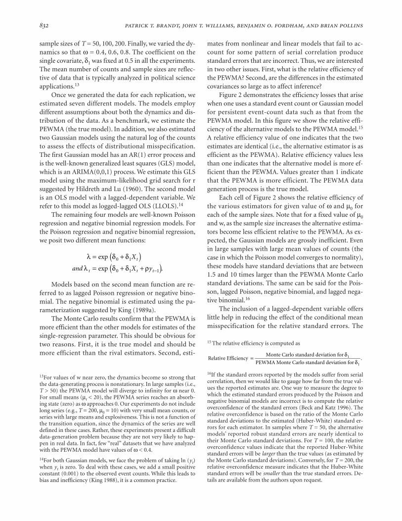
Figure 2 demonstrates the efficiency losses that arisewhen one uses a standard event count or Gaussian modelfor persistent event-count data such as that from thePEWMA model. In this figure we show the relative effi-ciency of the alternative models to the PEWMA model.15

A relative efficiency value of one indicates that the twoestimates are identical (i.e., the alternative estimator is asefficient as the PEWMA). Relative efficiency values lessthan one indicates that the alternative model is more ef-ficient than the PEWMA. Values greater than 1 indicatethat the PEWMA is more efficient. The PEWMA datageneration process is the true model.

Each cell of Figure 2 shows the relative efficiency ofthe various estimators for given value of ω and µ0 foreach of the sample sizes. Note that for a fixed value of µ0

and w, as the sample size increases the alternative estima-tors become less efficient relative to the PEWMA. As ex-pected, the Gaussian models are grossly inefficient. Evenin large samples with large mean values of counts (thecase in which the Poisson model converges to normality),these models have standard deviations that are between1.5 and 10 times larger than the PEWMA Monte Carlostandard deviations. The same can be said for the Pois-son, lagged Poisson, negative binomial, and lagged nega-tive binomial.16

The inclusion of a lagged-dependent variable offerslittle help in reducing the effect of the conditional meanmisspecification for the relative standard errors. The

13For values of w near zero, the dynamics become so strong thatthe data-generating process is nonstationary. In large samples (i.e.,T > 50) the PEWMA model will diverge to infinity for ω near 0.For small means (µt < 20), the PEWMA series reaches an absorb-ing state (zero) as ω approaches 0. Our experiments do not includelong series (e.g., T = 200, µ0 = 10) with very small mean counts, orseries with large means and explosiveness. This is not a function ofthe transition equation, since the dynamics of the series are welldefined in these cases. Rather, these experiments present a difficultdata-generation problem because they are not very likely to hap-pen in real data. In fact, few “real” datasets that we have analyzedwith the PEWMA model have values of ω < 0.4.

14For both Gaussian models, we face the problem of taking ln (yt)when yt is zero. To deal with these cases, we add a small positiveconstant (0.001) to the observed event counts. While this leads tobias and inefficiency (King 1988), it is a common practice.

15 The relative efficiency is computed as

Relative Efficiency

Monte Carlo standard deviation for

PEWMA Monte Carlo standard deviation for = δ

δ1

1

.

16If the standard errors reported by the models suffer from serialcorrelation, then we would like to gauge how far from the true val-ues the reported estimates are. One way to measure the degree towhich the estimated standard errors produced by the Poisson andnegative binomial models are incorrect is to compute the relativeoverconfidence of the standard errors (Beck and Katz 1996). Therelative overconfidence is based on the ratio of the Monte Carlostandard deviations to the estimated (Huber-White) standard er-rors for each estimator. In samples where T = 50, the alternativemodels’ reported robust standard errors are nearly identical totheir Monte Carlo standard deviations. For T = 100, the relativeoverconfidence values indicate that the reported Huber-Whitestandard errors will be larger than the true values (as estimated bythe Monte Carlo standard deviations). Conversely, for T = 200, therelative overconfidence measure indicates that the Huber-Whitestandard errors will be smaller than the true standard errors. De-tails are available from the authors upon request.

-

lagged Poisson and lagged negative binomial models arealways more efficient than the standard Poisson andnegative binomial regressions. These lagged count mod-els are generally less efficient than the PEWMA. It isworth reiterating that using lagged-dependent counts inthe negative binomial and Poisson regression modelsprovides a poor method of accounting for time-seriesproperties.17 The implication of estimating incorrect

standard errors with Poisson and negative binomial re-gressions should not be understated. The results demon-strate that the degree of inefficiency is large for a varietyof sample sizes, means, and varying degree of dynamics.

FIGURE 2 Relative Efficiency of Various Alternative Estimators to the PEWMA

Each line corresponds to a relative efficiency of the estimator to the PEWMA estimator. Each box in the figure shows the relative efficiency of the estima-tor (each line) to the PEWMA for a given value of ω and µ. The rows of the figure show the variation in the relative efficiency for the different values of µ fora given value of ω. The columns show the variation in relative efficiency for different values of ω for a given value of µ. We have indicated the relative effi-ciency value of 1 by a horizontal line in this plot. See text for discussion.

50 100 150 200 50 100 150 200

50 100 150 200

0

2

4

6

8

10

0

2

4

6

8

10

0

2

4

6

8

10

10 50

10 50

10 50

0.4 0.4

0.6 0.6

0.8

N

20

20

20

0.4

0.6

0.8 0.8

Logged-Lagged OLS

Gaussian AR(1) Errors

Poisson

Lagged Poisson

Negative Binomial

Lagged Negative Binomial

17 We also computed the Monte Carlo estimates for the dynamicand dispersion parameters: ω in the PEWMA, the autocorrelationparameter ρ for the ARIMA, LLOLS, the lagged Poisson, and

lagged negative binomial models, and the dispersion parameter forthe negative binomial models. The estimate of ω in the PEWMAmodels is almost always significant for the experiments. In almostevery case, the hypothesis that the Poisson regression is the truemodel is rejected based on a t-test for omega (H0 : ω = 1; HA :ω < 1). However, there is a small upward bias in the small sampleestimates of ω and this parameter should be interpreted carefully.Details of these results are available upon request.

. , . , . ,

Application: Pollins’s CoevolvingSystems Analysis

In order to demonstrate the important practical conse-quences of using the PEWMA rather than a lagged Pois-son regression model (LP), we present a revision ofPollins’s (1996) analysis of how variations in global po-litical and economic activity affect armed conflict. Wethen reestimate Pollins’s models using the PEWMA esti-mator. We show that the LP results reported in Pollins(1996) underestimate the standard errors of the param-eters, leading to overly optimistic conclusions about sev-eral of the theoretical models he tests. We find that thePEWMA dominates the LP model in terms of both effi-ciency and the Akaike Information Criterion (AIC).

Our replication of Pollins’s (1996) analysis of howcycles in global economic activity and the global politicalorder affect armed conflict demonstrates that accountingfor the temporal dependence in the data leads to differentconclusions about hypothesis tests of the causes of inter-national conflict. The problem with standard approachessuch as the lagged Poisson regression is that serial depen-dence in the data lead to incorrect standard errors. Thisleads to incorrect inferences since Pollins’s statistical testsare based on these erroneous standard errors.

The time dimension figures prominently in thetheories tested by Pollins, including the new model of“Coevolving Systems” he develops out of his analysis. Inhis analysis, international relations theories of armedconflict and war are explained by these theories in part asa function of overarching systemic conditions tied tochanges over time in the global economy and world or-der. Pollins notes five major theories that have been pro-posed to explain the patterns of armed conflict and war.Long Wave theories (Goldstein 1988, 1991) map long-term, repeated phases of growth and stagnation in theglobal economy. Wallerstein (1983) interprets these eco-nomic patterns as tied to the rise and fall of a single,dominant state, or “hegemon” in the system. Modelskiand Thompson (1987, 1996) interpret growth and de-cline as tightly connected to a century-long process theyterm the Leadership Cycle, and Gilpin (1981) argues thatthe ascendance of hegemons like Great Britain in theNineteenth Century and the United States in the mid-Twentieth Century brings a period of lower armed con-flict and relative peace. The phenomena of interest tothese scholars unfold over periods of fifty to a hundredyears or more. Pollins (1996) notes the Long Wave andthe Leadership Cycle and develops a model that accountsfor the separate effects which they may have on the gen-eration or suppression of conflict at any moment in time.

He then tests each of the five theories against the samedata on military disputes. The data consist of annualevent counts of the number of Militarized Interstate Dis-putes assembled by the Correlates of War project. Thesedata span the years 1816–1976, yielding 161 observationsin this event-count series. Pollins estimates a lagged Pois-son regression model consistent with each theory basedon the following model:

Pr |!

exp ,

Ye

y

Y X M

t tty

t

t t t t

t t

λ λ

λ ρ δ ζ

λ( ) =

= + +( )

−

−1

where λt is the mean of the Poisson random variable, Yt–1

is a lagged endogenous count, Xt is a 1 × K matrix ofphase parameters for the different model specifications,and Mt is the number of members in the interstate sys-tem in period t.18

Pollins recognizes time dependence in the Disputedata series on theoretical grounds. He argues that there isa degree of inertia in peace and conflict in the interna-tional system, thus the level of conflict in any year willhelp predict the level of conflict in the subsequent year.Moreover, the number of disputes observed in any yearshould correlate with the number of states in the system,for the simple reason that opportunities for conflict willvary with system size. Pollins makes use of this informa-tion in his specification of all five models as well as in a“Sophisticated Null” model which becomes his bench-mark for comparison for the five contending Long Cyclespecifications (Pollins, 1996, 109–110). This null modelpredicts the annual number of Disputes using a laggedendogenous variable (to represent the inertia, orautocorrelation effect) and the number of states in thesystem that year (which, given that this number risesthrough history, serves as a kind of trend component inthe time series).

Based on this model, Pollins estimates six differentspecifications for Xt based on the theories of Gilpin,Wallerstein, Goldstein, Modelski and Thompson, hisown “Coevolving Systems,” as well as a “SophisticatedNull” model to explain the presence of economic or lead-ership cycles in international disputes. The SophisticatedNull model contains only the lagged count and the num-ber of members in the interstate system (attempting tocapture autocorrelation and trend effects, respectively)and no other Xt.

The results of the Pollins’s study show that eachmodel passes statistical muster, despite their differences

18All variable definitions follow those used in Pollins (1996).

-

in approach and some conflicting claims between them.Each of the five models passes a likelihood ratio testagainst the “Sophisticated Null” model driven only bytwo trend components (lagged Militarized Interstate Dis-putes and the number of members in the internationalsystem), while the estimated parameters for each modelare found to be consistent with most of the hypothesesgenerated by that particular model. Some models cap-ture more of the variation in the annual dispute countthan others, and Pollins shows that his Coevolving Sys-tems model captures substantially more of this variationthan any other contender.

Pollins’s theoretical argument about inertia in thelevel of international conflict leads him to the laggedPoisson specification. Based on the earlier results, thiscorrection is not advised for two reasons. First, the LP co-efficient for the lagged dependent variable captures onlythe growth rate of the series. If an event-count time seriesis persistent but mean-reverting, the lagged Poissonmodel will have an estimated coefficient of zero for thelagged dependent variable. Since the model only capturesexponential deterministic trends, it has limited applica-bility in most cases.19 Second, the Monte Carlo analysisshows that simply including a lagged endogenous vari-able as a regressor in the standard Poisson regressionmodel is a poor correction for the inefficiency inducedby persistent serial dependence. Thus, more efficient esti-mates should be obtained with the PEWMA model.

Our reassessment of these five theoretical modelsuses three criteria: First, does the model in question fit thedata better than the “Sophisticated Null” specification?Because this null model is nested within each of Pollins’sfive specifications, the log-likelihood ratio test may beused to answer this question. We therefore estimate a “So-phisticated Null” model using the PEWMA, including thenumber of states in the system as the only regressor, sincethe dynamics are captured by the weighting term ω. Sec-ond, are the hypotheses generated by each theoreticalmodel supported by the PEWMA parameter estimatesand standard errors? Here we will find whether theLagged Poisson estimates presented in Pollins (1996) wereoverly optimistic in the inferences they produced. Third,does any one of these models perform better than allothers? Because the Gilpin, Wallerstein, Modelski andThompson, Goldstein, and Pollins models are nonnested,

the log-likelihood ratio test is not appropriate for com-parisons between them. Instead, we look to the Akaike In-formation Criterion (AIC) as the appropriate standard forcomparing the relative fit and parsimony of these non-nested models.

We begin our reanalysis of Pollins’s models by firstassessing the time-series properties of the disputes series.Figure 3 presents a plot of the original data and the auto-correlation function for the Disputes series.

It is clear from the figure that the Disputes series ishighly persistent. Thus, models with a fixed mean such asthe standard Poisson regression or standard negative bi-nomial regression will fail to account for the change in themean over time. While an LP model may explain the trendin the data, it is highly unlikely that the growth in thenumber of Disputes has a deterministic growth rate asimplied by this model. Rather, the more likely scenario isa stochastic trend, similar to that implied by the PEWMA.

The results of our reestimations using the PEWMAand LP are presented in Table 1.20 We begin our compari-son of Lagged Poisson and PEWMA estimates of thesesix models by comparing the model parameters and as-sociated standard errors produced by these two estima-tors (i.e., results for the five theoretical models and the“Sophisticated Null”). As for the model parametersthemselves, relatively little change is observed. Only fourof the twenty-seven parameters reestimated for thesemodels changed by more than 30 percent. Nine changedby less than 10 percent. This essential stability in the co-efficients is not surprising given that the LP and PEWMAestimators are in the same linear exponential family ofestimators.

The estimated standard errors show a more distinc-tive pattern. Downward bias in the LP estimated standarderrors is indicated, as all but two of the PEWMA standarderrors are larger, and most are larger by 30 percent ormore. The source of this bias is the failure to account forthe time series properties of the Disputes series. This isconsistent with the Monte Carlo findings that the LP esti-mates produce “overconfident” results (see footnote 16).

Inferences about the theories are affected; the statis-tical significance of individual model parameters is lowerin the PEWMA results, but still strong enough in thiscase to pass widely accepted criterion (p < .05). However,the central theoretical arguments put forward in Pollins(1996) depend not on the significance of individual coef-ficients, but on the differences between particular coeffi-cients. For any one of the models tested by Pollins, the

19For the Correlates of War Disputes data used by Pollins, the se-ries has a growth rate of approximately 1 percent. This is consistentwith his earlier estimates. Taking first differences, the data is sta-tionary. Specification as a deterministic trend is highly unlikely, asmost economic and social science series exhibit stochastic trends(Nelson and Plosser 1982).

20The “Lagged Poisson” results presented in Table 1 represent asuccessful replication of the results presented in Pollins (1996).

. , . , . ,

FIGURE 3 Militarized Interstate Disputes Series and Autocorrelation Function, 1816–1976

Year

Dis

put

es C

ount

1820 1840 1860 1880 1900 1920 1940 1960 1980

05

1015

2025

AC

F

–1.0

–0.5

0.0

0.5

1.0

1 2 3 4 5 6 7 8

Lag

9 10 11 12 13 14 15

coefficient associated with the system phase (e.g., Vic-tory, Maturity, Decline, and Ascent in the Wallersteinmodel) represents the effect on the expected annualnumber of armed Disputes within the phase. If the cyclephases are to predict the level of conflict in the interna-tional system, then the expected level of conflict (whosepoint-estimate is the phase parameter) should changesignificantly as the world moves from one period to thenext (e.g., from Victory to Maturity, and so on).

The PEWMA results suggest that the claims found inPollins (1996) regarding models other than his own areoverconfident. While the LP estimates of the Wallerstein,Modelski and Thompson, and Goldstein formulationsindicated reasonable evidence of cycles, most of that evi-dence disappears in the PEWMA estimates. In Table 1,only two of the twelve phase transition tests for thesethree models are now significant, rather than seven oftwelve as estimated by the LP. Claims for the Pollinsmodel are only slightly weaker than originally reported.

The PEWMA estimates show that four of the six hypoth-eses regarding phase transition are substantiated ratherthan six of six as estimated by the LP. Given the PEWMAresults, the Pollins model has difficulty in distinguishingbetween periods when the lowest levels of conflict arepredicted (periods CR2 and CR3). The model’s ability todistinguish between periods predicting medium andhigh levels of conflict remains significant.

The LP and PEWMA results yield very different an-swers concerning overall model adequacy. Pollins (1996)reports that each of the five models tested is shown supe-rior to the null model, based on the log-likelihood ratiotest using the LP estimates (the Wallerstein model is sig-nificant just above the 0.05 level in our replication).From the PEWMA estimates only, Pollins’s “CoevolvingSystems” model is shown to be superior to the nullmodel by this same test. We also compared the PEWMAresults for these models using the Akaike InformationCriterion (AIC). Pollins’s model exhibited the lowest

-

TABLE 1 Comparison of Lagged Poisson and PEWMA Results

Transition Tests Log-LikelihoodModel and Phases Parameters Standard Errors for Phase Shifts Ratio Tests AIC

LP PEWMA LP PEWMA LP PEWMA LP PEWMA LP PEWMANull Model 761.2 730.4

Gilpin 744.5 736.1

UK .67 .95 .08 .32Interregnum 1.08 1.00 .08 .17 *US 1.17 .87 .11 .20Members .005 .008 .001 .006Lag .07 .01ω .67 .04

Wallerstein 757.9 734.1

Victory .80 1.02 .08 .16 *Maturity .78 .51 .10 .14 *Decline .58 .49 .13 .17 *Ascent .99 .82 .12 .18Members .07 0.011 .01 0.006Lag .01 .002ω .68 .04

Modelski and Thompson * 753.1 736.7

World Power .61 .54 .10 .15Delegitimation .67 .70 .11 .18 *Deconcentration .87 .76 .08 .20Global War .94 .88 .09 .17 *Members .06 0.009 .01 0.006Lag .01 .002ω .68 .04

Goldstein * 749.1 734.2

Stagnation .64 .65 .10 .14 *Rebirth .86 1.00 .10 .13 *Expansion 1.07 .98 .09 .11War 1.10 1.06 .11 .11 * *Members .06 .01 .01 .006Lag .01 .001ω .70 .05

Pollins * * 714.6 725.0

CR2 -.02 .42 .24 .42 *CR3 .56 .72 .12 .15 *CR4 .94 .72 .11 .12 * *CR5 .75 .50 .11 .12 * *CR6 1.20 1.15 .09 .12 * *CR7 .85 .83 .12 .11 * *CR8 1.46 1.34 .14 .19 n.a. n.a.Members .04 .01 .01 .003Lag .01 .002ω .83 .06

Notes: * indicates significance at the 0.05 level or better for given test. The “Transition Test” is a t-test of successive phase coefficients, described in textand in Pollins (1996) footnote 17 as amended. The test checks for significant shift in frequency of Disputes as system moves from one phase to another.The log-likelihood ratio tests are conducted for each model against the LP and PEWMA “Sophisticated Null,” respectively. The “AIC” is the Akaike Infor-mation Criterion for fit and parsimony. Lower values are superior. All of the estimated coefficients except for “CR2” are significant at the 0.05 level.

. , . , . ,

(i.e., best) AIC of all tested and was the only theoreticalformulation to show itself superior to the null model.

The results of our replication of the Pollins studyshed additional light on the PEWMA estimator and onthe models and substantive claims examined in that ear-lier study. First, consistent with the Monte Carlo exami-nation of the PEWMA estimator, we find that the modelparameters tended to change only moderately, while esti-mated standard errors increased in most instances. Thisrevised (and we believe more accurate) picture of thestandard errors is sufficient to change several conclusionsfrom the study we replicated.

Second, using the PEWMA we did not find all fivetheoretical models to be superior to the null model. OnlyPollins’s “Coevolving Systems” model passed the likeli-hood ratio test, and only this same model had a lowerAIC than the null model. And once we took direct ac-count of the dynamics in the Dispute time series (repre-sented by the weighted moving average coefficient, ω),only the Pollins model showed multiple phase transitionsas hypothesized. Our revised results underscore the callmade by Pollins (1996: 116) for deeper specification ofthe separate contributions made by the Leadership Cycleand the Long Wave to the generation of armed conflict.

Third, we do find support for Pollins’s claim that the“Coevolving Systems” model can extend these frame-works to understanding conflict patterns beyond thislimited domain by taking account of independent effectsof the Long Wave and the Leadership Cycle. His call forfuture research in this area to follow his approach is con-sistent with our PEWMA findings. The Pollins modelwas the only one among the five to show improvementover the null model (by both the log-likelihood and AICcriteria) and the only model to exhibit a number of sig-nificant changes in Dispute frequencies from one phaseto the next.

In sum, the PEWMA reanalysis of the Pollins (1996)study does not resolve all debates in long-cycle research.But it does demonstrate quite clearly that proper model-ing of the dynamic properties of event time series is keyto model specification and theory testing. And direct es-timation of these dynamic properties, as contained in themoving average parameter (ω), should be the preferredapproach for those modeling event count time series.

Conclusion

The PEWMA model offers a straightforward and easilyestimable (and interpretable) method for modelingevent-count data with persistent dynamics. Our experi-

ence is that many event-count time series are persistent.Indeed, persistence is probably the most common featurewe have found in time-series event counts. However,many series also exhibit independence, and for those casesthe Poisson or negative binomial models are appropriate.

An alternative situation is when data have dynamicsbut are mean reverting. The proper specification for sucha case is an autoregressive model (see Brandt and Will-iams 1998). Thus, PEWMA is not always the best modelfor time-series event counts, but it will often be so. Ana-lysts of event-count data need a more complete tool bagthan they now have. The PEWMA is an important addi-tion to the tools of political scientists.

Our Monte Carlo experiments indicate significantefficiency losses occur when event-count time series dataare modeled using either Poisson or negative binomialassumptions. Since most political scientists are trying toexplain events with covariates, our focus has been on theloss of efficiency of coefficients on covariates. There isevery reason to believe that if persistence in data is ig-nored, not only will estimates be inefficient, but reportedconfidence intervals from Poisson and negative binomialmodels will be much too small. This means that scientificjudgments can be seriously flawed.

Also, our PEWMA model is easy to specify and esti-mate. We have written and made available software forestimating this model. As noted earlier, the software is asfast as standard estimation algorithms for Poisson andnegative binomial regression models currently used inpolitical science. We will be making a standalone versionof this software available as part of an updated version ofKing’s (1994) COUNT program.21

Finally, the PEWMA reanalysis of the Pollins studyunderscores the importance of properly modeling thedynamic properties of event-count time-series data. Thelagged Poisson specification Pollins originally employedproduced results that differed in substantively importantways from those the PEWMA model generated. UnlikePollins, most previous research using time-series event-count data does not attempt to model the dynamics ofthese data at all. Since even an inadequate specification ofthe dynamics can produce somewhat misleading results,there is every reason to suspect that failing to considerthem at all poses a grave threat to the validity of the re-sults. The PEWMA model offers a relatively simple wayto model the dynamics of persistent event-count seriesand thus to avoid these problems.

21Both the Gauss source code and the stand-alone program can befound at http://www.polsci.indiana.edu/jotwilli/home/default.htm.

-

Appendix APEWMA Filtering Algorithm and

Predictive Distribution

The PEWMA uses a version of the Kalman filter to estimatea time-varying mean for event-count data. This filter can bederived using the three basic assumptions that define thePEWMA model, in equations (1)–(4).

The filter computes three quantities: the unconditionalmean of the process ( [ | ])E Yt tµ − −1 1 , the conditional mean ofthe process ( [ | ])E Yt tµ −1 , and the posterior mean of the pro-cess ( [ | ])E Yt tµ . Similar to Gaussian ARIMA models theKalman filter for count data requires that E Yt t[ | ]µ −1

= − −E Yt t[ | ]µ 1 1 , and Var Y Var Yt t t t[ | ] [ | ]µ µ− − −>1 1 1 . In words,the conditional mean in periods t and t – 1 is equal, but theconditional variance for period t is larger. This effect isachieved in the gamma distribution by using thehyperparameter ω ∈ (0,1] to discount the value of past ob-servations in the computation of E Yt t[ | ]µ −1 . The conjugacyassumption ensures that the mean of the gamma distribu-tion is the same in each period, but that the conditional pre-dictive variance in period t is larger than in period t – 1.This effect is induced by multiplying µt–1 by a factor lessthan 1 in the transition equation (2).

To derive the Kalman filter equations for the PEWMA,we compute the prior, conditional, and posterior mean.First, substituting the gamma prior (4) into the transitionequation (3) yields

µ µ ηη δ

t tr

t

t t

tt t

e

a

bX r

t=

= +

−

−

−

1

1

1

exp( ).

Conditional on Yt–1, µt is gamma distributed and we write

µt t t t t tY a b| ~ ( , )| |− − −1 1 1Γ . This is the prior mean of the pro-cess at time t.

From the properties of the gamma distribution, µt tY| −1

has a gamma distribution with parameters at t| −1 and bt t| −1

such that

a at t t| − −=1 1ω and (9a)

b b X rt t t t t| exp( ), ( , ]− −= − − ∈1 1 0 1ω δ ω . (9b)

Based on the properties of the gamma distribution, we canthen calculate E Yt t[ | ]µ −1 and Var Yt t[ | ]µ −1 :

E Y

a

b

a

b X rE Yt t

t t

t t

t

t t tt t[ | ]

exp( )[ | ]|

|

µδ

µ−−

−

−

−− −= =

− −=1

1

1

1

11 1 (10)

and

Var Ya

b

a

b X rt t

t t

t t

t

t t t

[ | ]( ) exp( )

|

|

µ ω

ω δ−

−

−

−

−

= =− −( )1

1

12

1

21

22

=−

− −ω µ11 1Var Yt t[ | ] (11)

These are the conditional mean and variance of theprocess and the mean and variance conditions demandedabove are satisfied. When ω = 1, this model is the Poissonmodel since the mean and variance of the model will beequal. In this case, the conditional Poisson distribution hasa fixed mean, so the value of at–1/bt–1 is absorbed in the con-stant term of the Poisson regression model.

To evaluate these quantities and derive the posterior dis-tribution, we need a formula for computing rt. Recall fromequation (7) that the transition equation can be written

ln( ) ln( ) ln( )µ µ ηt t t tr− = +−1

where µt is the conditional mean, rt is the per period growthrate, and ηt are the errors. The left-hand side of this equa-tion is an estimate of the growth rate of the series of eventcounts. The right-hand side is the growth rate, plus a sto-chastic component. The left-hand side of this equation iszero in expectation, since we constructed E Yt t[ | ]µ − −1 1 =

E Yt t[ | ]µ −1 and the model has a zero growth rate. Therefore,since ht follows a beta distribution, this expectation can beevaluated using an integral formula:

r E

B a ad

B a a

t t

t t

at

at t

t tt

at

a

t t

t t

= −

= −−

−

= −−

−

− −

− − −

− −

− − −

∫

∫

− −

− −

[ln( )]

( ,( ) )( ) ln( )

( ,( ) )( ) ln(

( )

( )

η

ω ωη η η η

ω ωη η η

ω ω

ω ω

1

11

1

11

1 10

1 1 1 1

1 1

10

1 1 1

1 1

1 1tt t

t t

d

a a

)

( ) ( ),

η

ω= −− −Ψ Ψ1 1

where B(·,·) is the beta function and Ψ Γ

( )ln ( )⋅ = ∂∂

x

x is

Euler’s psi or digamma function. This expectation can benumerically evaluated using standard approximations forthe digamma function (Abramowitz and Stegun, 1972).

In order to make use of the structural model, we need tobe able to compute the posterior of µt once Yt is available.This will allow us to construct the predictive distribution,

Pr( | )y Yt t −1 , and likelihood function, Pr( , | , )ω δ y y XT t1K .We compute the posterior using Bayes rule. Given the ob-served count yt we update the conditional values of

a bt t t t t t| | |, ,− − −1 1 1 µ to find µt tY| using Bayes rule:

. , . , . ,

Pr( | )Pr( | ) Pr( )

Pr( | ) Pr( )

| ||

|

|

µ µ µ

θ θ θ

µµ

t tt t t

t

b y at t

y a

t t t

YY

Y d

e b

y a

t t t t t tt t

= ⋅

⋅

=+( )

+( )

∞

− +( ) + −−

− +( )

−

∫

− −−

0

1 11

1

1 11

1

Γ

where Γ refers to the gamma function. This is a gamma dis-tribution, µt t t t t t tY a y b| ~ ( , )| |Γ − −+ +1 1 1 . Then, the posterior

Pr( | )µt tY is given by a gamma distribution with param-eters generated by the recursions,

a a y a yt t t t t t= + = +− −| 1 1ω and (13a)

b b b X rt t t t t t= + = + +− −| exp( ),1 11 ω δ (13b)

where (13b) follows from a renormalization of the scale ofthe gamma distribution. These recursions and the set of ini-tial values define a Kalman filter for the count data with aPoisson measurement equation and a gamma-distributedprior. The filter is defined by the recursive system of equa-tions (9a–13b).

Since the gamma is the natural conjugate distribution ofthe Poisson, the resulting predictive distribution and likeli-hood are in the same family of distributions as the Poisson.This predictive distribution is a Poisson with a gammaprior,

Pr( | ) Pr( | ) Pr( | )

( )

! ( )exp( )

exp( )( )

y Y y Y d

y a

y ab X r

b X r

t t t t t t t

t t

t tt t t

a

t t t

y a

t

t t

−∞

−

−

−−

−− +

=

= + − −( )× + − −( )

∫−

−

1 0 1

1

11

1

1

11

µ µ µ

ωω

ω δ

ω δ

ω

ω

ΓΓ

(14)

where at–1, bt–1, and rt are based on the filter computations.This is a negative binomial distribution.22

The filter parameters can then be used to compute thepredictive distribution and maximum-likelihood estimatesin equations (6) and (14).

Appendix BPEWMA Forecasts and Predictions

The forecast function for the PEWMA model is derivedgiven estimates of ω and δ. From the properties of the nega-tive binomial distribution the mean and variance of the pre-dictive distribution at time T + 1 are obtained from the fil-ter parameters:

E y Y

a

b

a y

b

a y

b X rT TT

T

T T T

T T

T T

T t t

( | )exp( )

|

|+

+

+= = +

+= +

+ +11

1 1

ωω δ

, and

(15)

V y Y

a b

bV Y E YT T

T T T T

T TT T T T( | )

( )( | ) ( | )| |

|+

+ +

+

−= + = +11 1

12

11 ω µ µ ,

(16)

where aT and bT are the posterior gamma distribution pa-rameters computed by the filter.

Based on repeated substitutions of at–1, at t| −1, at , bt–1,

bt t| −1, bt (from the filter computations) the forecast functionfor the one-step ahead prediction is:

y X ry

X rT T T T

jT jj

T

jjT

T j T j

T T+ + +−=

−

=−

− −+= +

+=

∑∑

1 1 101

01 1| |exp( )

exp( )δ

ω

ω δµ .

(17)

This forecast function has a natural interpretation in thecontext of known time-series models. The forecast condi-tions the observation in period T + 1 on the realizations ofpast observations, as well as the covariates that enter themodel multiplicatively according to (2). The forecast meanlevel is a discounted weighted average of past observations,where the weights decline exponentially. The forecast func-tion produces estimates that follow an exponentiallyweighted moving average (EWMA) (Harvey 1989, 25–26).When T is large, yt t+1| approaches ω ωy yt t t| ( )− + −1 1 for t =1, . . . , T. This is the limiting form of the EWMA for µt t+1| .

Multi-step prediction requires integration of the condi-tional density function, equation (14). Thus, the multi-steppredictions cannot be found by a simple additive recursionas in the Gaussian model. The l-step ahead predictive dis-tribution is

Pr( | ) Pr | ) Pr( | )y Y y YT T T T T T T+ + +

∞+ += ⋅ ∂∫l l l l l( µ µ µ

0(18)

Simply using the recursions (9a–13b) ignores the evolu-tion of µt for observations at T + 1, T + 2, . . . , T + l – 1.

22A proper distribution for µt requires that µt ≠ 0. Thus, we set t =τ where τ is the time of the first non-zero observation. In practice,we initialize the filter at t = 0 using the sample mean of the seriesfor µ0. The prior becomes diffuse as a and b approach zero. Al-though the gamma distribution is degenerate in this case, a = b =0 implies that Pr(µ = 0) = 1. The distribution of µt is then properlydefined at t = τ where τ is the first nonzero observation (Harveyand Fernandes 1989, 408). This can be easily implemented by re-moving the first t – 1 zero observations from the data.

-

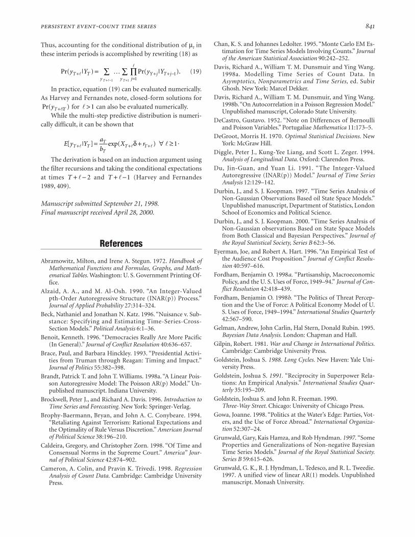
Thus, accounting for the conditional distribution of µt inthese interim periods is accomplished by rewriting (18) as

Pr( | ) Pr( | ).y Y y YT T

yY j T j

jyT T

+ + + −=

=+ − +

∑ ∏∑l

l

Kl 1 1

11

(19)

In practice, equation (19) can be evaluated numerically.As Harvey and Fernandes note, closed-form solutions for

Pr( )|yT T+l for l >1 can also be evaluated numerically.While the multi-step predictive distribution is numeri-

cally difficult, it can be shown that

E y Y

a

bX rT T

T

TT T[ | ] exp( )+ + += + ∀ ≥l l l lδ 1.

The derivation is based on an induction argument usingthe filter recursions and taking the conditional expectationsat times T + −l 2 and T + −l 1 (Harvey and Fernandes1989, 409).

Manuscript submitted September 21, 1998.Final manuscript received April 28, 2000.

References

Abramowitz, Milton, and Irene A. Stegun. 1972. Handbook ofMathematical Functions and Formulas, Graphs, and Math-ematical Tables. Washington: U. S. Government Printing Of-fice.

Alzaid, A. A., and M. Al-Osh. 1990. “An Integer-Valuedpth-Order Autoregressive Structure (INAR(p)) Process.”Journal of Applied Probability 27:314–324.

Beck, Nathaniel and Jonathan N. Katz. 1996. “Nuisance v. Sub-stance: Specifying and Estimating Time-Series-Cross-Section Models.” Political Analysis 6:1–36.

Benoit, Kenneth. 1996. “Democracies Really Are More Pacific(In General).” Journal of Conflict Resolution 40:636–657.

Brace, Paul, and Barbara Hinckley. 1993. “Presidential Activi-ties from Truman through Reagan: Timing and Impact.”Journal of Politics 55:382–398.

Brandt, Patrick T. and John T. Williams. 1998a. “A Linear Pois-son Autoregressive Model: The Poisson AR(p) Model.” Un-published manuscript. Indiana University.

Brockwell, Peter J., and Richard A. Davis. 1996. Introduction toTime Series and Forecasting. New York: Springer-Verlag.

Brophy-Baermann, Bryan, and John A. C. Conybeare. 1994.“Retaliating Against Terrorism: Rational Expectations andthe Optimality of Rule Versus Discretion.” American Journalof Political Science 38:196–210.

Caldeira, Gregory, and Christopher Zorn. 1998. “Of Time andConsensual Norms in the Supreme Court.” America” Jour-nal of Political Science 42:874–902.

Cameron, A. Colin, and Pravin K. Trivedi. 1998. RegressionAnalysis of Count Data. Cambridge: Cambridge UniversityPress.

Chan, K. S. and Johannes Ledolter. 1995. “Monte Carlo EM Es-timation for Time Series Models Involving Counts.” Journalof the American Statistical Association 90:242–252.

Davis, Richard A., William T. M. Dunsmuir and Ying Wang.1998a. Modelling Time Series of Count Data. InAsymptotics, Nonparametrics and Time Series, ed. SubirGhosh. New York: Marcel Dekker.

Davis, Richard A., William T. M. Dunsmuir, and Ying Wang.1998b. “On Autocorrelation in a Poisson Regression Model.”Unpublished manuscript, Colorado State University.

DeCastro, Gustavo. 1952. “Note on Differences of Bernoulliand Poisson Variables.” Portugaliae Mathematica 11:173–5.

DeGroot, Morris H. 1970. Optimal Statistical Decisions. NewYork: McGraw Hill.

Diggle, Peter J., Kung-Yee Liang, and Scott L. Zeger. 1994.Analysis of Longitudinal Data. Oxford: Clarendon Press.

Du, Jin-Guan, and Yuan Li. 1991. “The Integer-ValuedAutoregressive (INAR(p)) Model.” Journal of Time SeriesAnalysis 12:129–142.

Durbin, J., and S. J. Koopman. 1997. “Time Series Analysis ofNon-Gaussian Observations Based oil State Space Models.”Unpublished manuscript, Department of Statistics, LondonSchool of Economics and Political Science.

Durbin, J., and S. J. Koopman. 2000. “Time Series Analysis ofNon-Gaussian observations Based on State Space Modelsfrom Both Classical and Bayesian Perspectives.” Journal ofthe Royal Statistical Society, Series B 62:3–56.

Eyerman, Joe, and Robert A. Hart. 1996. “An Empirical Test ofthe Audience Cost Proposition.” Journal of Conflict Resolu-tion 40:597–616.

Fordham, Benjamin O. 1998a. “Partisanship, MacroeconomicPolicy, and the U. S. Uses of Force, 1949–94.” Journal of Con-flict Resolution 42:418–439.

Fordham, Benjamin O. 1998b. “The Politics of Threat Percep-tion and the Use of Force: A Political Economy Model of U.S. Uses of Force, 1949–1994.” International Studies Quarterly42:567–590.

Gelman, Andrew, John Carlin, Hal Stern, Donald Rubin. 1995.Bayesian Data Analysis. London: Chapman and Hall.

Gilpin, Robert. 1981. War and Change in International Politics.Cambridge: Cambridge University Press.

Goldstein, Joshua S. 1988. Long Cycles. New Haven: Yale Uni-versity Press.

Goldstein, Joshua S. 1991. “Reciprocity in Superpower Rela-tions: An Empirical Analysis.” International Studies Quar-terly 35:195–209.

Goldstein, Joshua S. and John R. Freeman. 1990.Three-Way Street. Chicago: University of Chicago Press.

Gowa, Joanne. 1998. “Politics at the Water’s Edge: Parties, Vot-ers, and the Use of Force Abroad.” International Organiza-tion 52:307–24.

Grunwald, Gary, Kais Hamza, and Rob Hyndman. 1997. “SomeProperties and Generalizations of Non-negative BayesianTime Series Models.” Journal of the Royal Statistical Society.Series B 59:615–626.

Grunwald, G. K., R. J. Hyndman, L. Tedesco, and R. L. Tweedie.1997. A unified view of linear AR(1) models. Unpublishedmanuscript. Monash University.

. , . , . ,

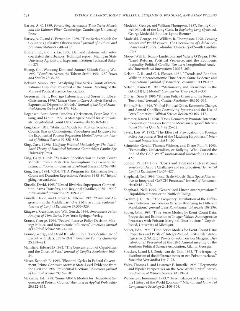
Harvey, A. C. 1989. Forecasting, Structural Time Series Modelsand the Kalman Filter. Cambridge: Cambridge UniversityPress.

Harvey, A. C., and C. Fernandes. 1989. “Time Series Models forCount or Qualitative Observations.” Journal of Business andEconomic Statistics 7:407–417.

Hildreth. C., and J. Y. Lu. 1960. Demand relations with auto-correlated disturbances. Technical report. Michigan StateUniversity Agricultural Experiment Station Technical Bulle-tin 276.

Huang, Chi, Woosang Kim, and Samuel Shiouh Guang Wu.1992. “Conflicts Across the Taiwan Strait, 1951–78.” Issuesand Studies 28:35–58.

Jackman, Simon. 1998. “Analyzing Time Series Counts of Inter-national Disputes.” Presented at the Annual Meeting of theMidwest Political Science Association.

Jorgensen, Bent, Rodrigo Labouriau, and Soren Lundbye-Christensen. 1996. “Linear Growth Curve Analysis Based onExponential Dispersion Models.” Journal of the Royal Statis-tical Society, Series B 58:573–592.

Jorgensen, Bent, Soren Lundbye-Christensen, Peter Xue-KunSong, and Li Sun. 1999. “A State Space Model for Multivari-ate Longitudinal Count Data.” Biometrika 86:169–181.

King, Gary. 1988. “Statistical Models for Political Science EventCounts: Bias in Conventional Procedures and Evidence forthe Exponential Poisson Regression Model.” American Jour-nal of Political Science 32:838–863.

King, Gary. 1989a. Unifying Political Methodology: The Likeli-hood Theory of Statistical Inference. Cambridge: CambridgeUniversity Press.

King, Gary. 1989b. “Variance Specification in Event CountModels: From a Restrictive Assumptions to a GeneralizedEstimator.” American Journal of Political Science 33:762–784.

King, Gary. 1994. “COUNT: A Program for Estimating EventCount and Duration Regressions, Versions 1988–94.” http://gking.harvard.edu.

Kinsella, David. 1995. “Nested Rivalries: Superpower Competi-tion, Arms Transfers, and Regional Conflict, 1950–1990.”International Interactions 21:109–125.

Kinsella, David, and Herbert K. Tillema. 1995. “Arms and Ag-gression in the Middle East: Overt Military Interventions.”Journal of Conflict Resolution 39:306–329.

Kitagawa, Genshiro, and Will Gersch. 1996. Smoothness PriorsAnalysis of Time Series. New York: Springer-Verlag.

Krause, George. 1994. “Federal Reserve Policy Decision Mak-ing: Political and Bureaucratic Influences.” American Journalof Political Science 38:124–144.

Krause, George, and David B. Cohen. 1997. “Presidential Use ofExecutive Orders, 1953–1994.” American Politics Quarterly25:458–481.

Mansfield, Edward D. 1992. “The Concentration of Capabilitiesand the Onset of War.” Journal of Conflict Resolution 36:3–24.

Mayer, Kenneth R. 1995. “Electoral Cycles in Federal Govern-ment Prime Contract Awards: State-Level Evidence fromthe 1988 and 1992 Presidential Elections.” American Journalof Political Science 39:162–185.

McKenzie, Ed. 1988. “Some ARMA Models for Dependent Se-quences of Poisson Counts.” Advances in Applied Probability20:822–835.

Modelski, George, and William Thompson. 1987. Testing Cob-web Models of the Long Cycle. In Exploring Long Cycles, ed.George Modelski. Boulder: Lynne Rienner.

Modelski, George, and William R. Thompson. 1996. LeadingSectors and World Powers: The Coevolution of Global Eco-nomics and Politics. Columbia: University of South CarolinaPress.

Moore, Will H., Ronny Lindstrom, and Valerie O’Regan. 1996.“Land Reform, Political Violence, and the EconomicInequality-Political Conflict Nexus: A Longitudinal Analy-sis.” International Interactions 21:335–363.

Nelson, C. R., and C. I. Plosser. 1982. “Trends and RandomWalks in Macroeconomic Time Series: Some Evidence andImplications.” Journal of Monetary Economics 10:139–162.

Nelson, Daniel B. 1990. “Stationarity and Persistence in theGARCH(1,1) Model.” Econometric Theory 6:318–334.

O’Brien, Sean P. 1996. “Foreign Policy Crises and the Resort toTerrorism.” Journal of Conflict Resolution 40:320–335.

Pollins, Brian. 1996. “Global Political Order, Economic Change,and Armed Conflict: Coevolving Systems and the Use ofForce.” American Political Science Review 90:103–117.

Remmer, Karen L. 1998. “Does Democracy Promote InterstateCooperation? Lessons from the Mercosur Region.” Interna-tional Studies Quarterly 42:25–52.

Sayrs, Lois W. 1992. “The Effect of Provocation on ForeignPolicy Response: A Test of the Matching Hypothesis.” Inter-national Interactions 18:85–100.

Schneider, Gerald, Thomas Widmer, and Dieter Ruloff. 1993.“Personality, Unilateralism, or Bullying: What Caused theEnd of the Cold War?” International Interactions 41:407–427.

Senese, Paul D. 1997. “Costs and Demands InternationalSources of Dispute Challenges and reciprocation.” Journal ofConflict Resolution 41:407–427.

Shephard, Neil. 1994. “Local Scale Models: State Space Alterna-tive to Integrated GARCH Processes.” Journal of Economet-rics 60:181–202.

Shephard, Neil. 1995. “Generalized Linear Autoregressions.”Unpublished manuscript. Nuffield College.

Skellam, J. G. 1946. “The Frequency Distribution of the Differ-ence Between Two Poisson Variates Belonging to DifferentPopulations.” Journal of the Royal Statistical Society 109:296.

Squier, John. 1997. “Time-Series Models for Event-Count Data:Properties and Estimation of Integer-Valued AutoregressiveProcesses with Poisson Marginal Distributions.” Unpub-lished, University of Michigan.

Squier, John. 1996. “Time-Series Models for Event-Count Data:Properties and Perils of Integer-Valued First-Order Auto-regressive (INAR(1)) Processes with Poisson Marginal Dis-tributions.” Presented at the 1996 Annual meeting of theSouthern Political Science Association, Atlanta, Georgia.

Strackee, J., and J. J. Denier van der Gon. 1962. “The frequencydistribution of the difference between two Poisson variates.”Statistica Neerlandica 16:17–23.

Volgy, Thomas J., and Lawrence E. Imwalle. 1995. “Hegemonicand Bipolar Perspectives on the New World Order.” Ameri-can Journal of Political Science 39:819–34.

Wallerstein, Immanuel. 1983. “Three Instances of Hegemony inthe History of the World Economy.” International Journal ofComparative Sociology 24:100–108.

-

Ward, Michael D., and Sheen Rajmaira. 1992. “Reciprocity andNorms in United States-Soviet Foreign Policy.” Journal ofConflict Resolution 36:369–385.

West, Mike, and P. Jeff Harrison. 1986. “Monitoring and Adap-tation in Bayesian Forecasting Models.” Journal of theAmerican Statistical Association 81(395):741–750.

West, Mike, and Jeff Harrison. 1997. Bayesian Forecasting andDynamic Models. New York: Springer-Verlag.

West, Mike, P. Jeff Harrison, and Helio Migon. 1985. “DynamicGeneralized Linear Models and Bayesian Forecasting (with

comments).” Journal of the American Statistical Association80:73–83.

Zeger, Scott L. 1988. “A regression model for time series ofcounts.” Biometrika 75:621–629.

Zeger, S. L., and B. Qaqish. 1988. “Markov Regression Modelsfor Time Series: A Quasi-Likelihood Approach.” Biometrics44:1019–1031.