MODELING THE FLOW OF A LIQUID DROPLET DIFFUSING INTO VARIOUS

POROUS MEDIA FOR INKJET PRINTING APPLICATIONS

By

SARAH ROSE SUFFIELD

A thesis submitted in partial fulfillment of the requirements for the degree of

MASTER OF SCIENCE IN MECHANICAL ENGINEERING

WASHINGTON STATE UNIVERSITY VANCOUVERSchool of Engineering and Computer Science

MAY 2008

ii

To the Faculty of Washington State University:

The members of the Committee appointed to examine the

dissertation/thesis of SARAH ROSE SUFFIELD find it satisfactory and recommend that

it be accepted.

iii

ACKNOWLEDGMENT

I would like to acknowledge and thank my advisor, Dr. Amir Jokar. I am very

grateful for the time he took to help me with this project. Without his guidance and

knowledge the completion of this thesis would not have been possible.

I would also like to thank my employer, HP, who provided financial support for

my graduate education. HP also provided me with the equipment resources required for

this project. I am also extremely appreciative of all the support I received from my

managers and coworkers. Without their understanding around my flexible work

schedule, completion of my masters degree would not have been possible.

iv

MODELING THE FLOW OF A LIQUID DROPLET IMPACTING WITH VARIOUSPOROUS MEDIA FOR INKJET PRINTING APPLICATIONS

Abstract

by Sarah Rose SuffieldWashington State University

May 2008

Chair: Amir Jokar

Inkjet technology currently relies heavily upon the absorption of ink into porous

media. Characterizing the absorption capacity of media as well as the absorption rate can

be critical in understanding the entire drying process. Evaluating the absorption

performance of a coated medium can particularly be important since the coating may be

either semi-absorptive, or in some cases non-absorptive. The absorption performance can

also vary among uncoated media. In order to better understand the absorption

mechanism, the fluid flow of a liquid droplet impacting with several porous papers, each

with a unique permeability was analyzed numerically and experimentally in this study.

The droplet impact was simulated by the computational fluid dynamics (CFD) technique

for a variety of conditions. The transient CFD modeling predicted the shape of the

droplet at different time intervals before and after the impact. It also predicted the

volume of liquid that had diffused into the porous substrate over time. The results

predicted by the CFD model were then compared to experimental data, which was

collected for a real system with the same configuration as in the CFD modeling, using a

high speed digital video camera. The camera captured images of a droplet as it impacted

with various coated and uncoated papers. Results showed a relatively good agreement

between the computational modeling and experimentation at drop times greater than 0.1

seconds after the impact. A dimensional analysis was also performed on the most

effective parameters of the flow process, and an imperial correlation was developed to

predict the aspect ratio of the droplet after the impact as a function of the other

dimensionless parameters, such as Reynolds and Weber numbers. The results of this

v

study can be useful for drying applications, such as inkjet printing, where absorption of a

liquid into a porous medium is critical for the drying process.

vi

TABLE OF CONTENTS

Page

ACKNOWLEDGEMENTS ………………………………………………………... iii

ABSTRACT ……………………………………………………………………….. iv

LIST OF TABLES ………………………………………………………………… ix

LIST OF FIGURES ……………………………………………………………….. . x

NOMENCLATURE …...………………………………………………………….. xii

CHAPTER

1. INTRODUCTION …………………………………………………….. . 1

2. LITERARY REVIEW ………………………………………………… . 4

Porosity and Permeability ………………………………………….. 4

Surface Tension ……………………………………………………...7

System Modeling …………………………………………………….7

3. CFD SIMULATION ..……………………………………….....……... 11

System Introduction ………………………………………………..11

System Geometry …………………………………………..12

Mesh ………………………………………………………………..12

Boundary Conditions ……………………………………………… 14

Fluent Models ……………………………………………………... 15

Fluent Solver ……………………………………………………….17

Input Data …………………………………………………………..18

Property Calculations ………………………………………………19

Porosity and Permeability ………………………………….19

Anisotropic Permeability ………………………………….. 23

Surface Tension ………………………………………….... 24

Droplet Velocity ……………………………………………………25

vii

Media ……………………………………………………………… 26

CFD Results ………………………………………………………..27

Volume of Water within Media ………..…………………. 27

Aspect Ratio …………………..…………………………... 29

4. EXPERIMENTAL TEST FACILITY ………………….…………….. 31

Experimental Schematic …………………………………………... 31

Syringe …………………………………………………………….. 33

Fixture ……………………………………………………………...33

Camera and Lens ………………………………………………….. 33

Other Equipment …………………………………………………...33

Test Procedure …………………………………………………….. 36

5. EXPERIMENTAL RESULTS AND COMPARISIONS …………...…37

Calculated Properties ……………………………………………… 37

Contact Angle ……………………………………………... 37

Average and Impact Velocity ……………….…………….. 38

Aspect Ratio ………………………………………………. 39

Data Comparisons ..………………………………………...39

6. DIMENSIONAL AND UNCERTAINTY ANALYSIS …………….... 45

Dimensional Analysis …………….……………………………….. 45

Derive Pi Terms …………………………………………… 46

Aspect Ratio Correlation ………….………………………..46

Uncertainty Analysis ……………………………………………….49

Uncertainty Results ………………………………………...50

7. SUMMARY AND CONCLUSIONS …………………………………. 52

BIBLIOGRAPHY ………………………………………………………………… 54

APPENDIX

A. INERTIAL RESISTANCE FOR UNCOATED MEDIA ...……………56

viii

B. SURFACE TENSION AT SUBSTRATE/AIR INTERFACE ………... 57

C. DIMENSIONAL ANALYSIS …………………………………………59

D. ASPECT RATIO CORRELATION …………………………………... 63

E. VISUAL BASIC CODE FOR UNCERTAINTY……………………....65

ix

LIST OF TABLES

1. Tabulated Permeability Data for Cellulose Fibers …………………………19

2. Media Set ………………………………………….………………………. 27

3. Average Contact Angle …………………………………………………… 38

4. Estimated Uncertainty of Parameters ………………………………………51

x

LIST OF FIGURES

1. Major Paper Directions …………………………………………………….. 6

2. Flow Diagram of a Droplet Impacting with a Porous Medium …………… 12

3. Model Geometry …………………………………………………………... 13

4. Typical Mesh Plot ………………………………………………………….14

5. Plot of Tabulated Cellulose Permeability Data …………………………… 20

6. Permeability Direction Vectors in Fluent Model …………………………. 24

7. Volume of Water Absorbed from the CFD Model for Uncoated Media …. 28

8. Volume of Water Absorbed from the CFD Model for Coated Media ……. 29

9. CFD Aspect Ratio for Uncoated Media …………………………………... 30

10. CFD Aspect Ratio for Coated Media ……………………………………... 30

11. Experimental Schematic …………………………………………………... 32

12. Close Up View of Syringe/Lens Setup ……………………………………. 32

13. Media Thickness Image of M2 ……………………………………………. 34

14. Coating Thickness Image of M1 …………………………………………...35

15. Fiber Diameter Image for M2 ……………………………………………...36

16. Contact Angle Image for M2 ……………………………………………… 37

17. Aspect Ratio Comparison of M1 ………………………………………….. 39

18. Aspect Ratio Comparison of M2 ………………………………………….. 40

19. Aspect Ratio Comparison of M3 ………………………………………….. 40

20. Aspect Ratio Comparison of M4 ………………………………………….. 41

21. CFD Model Aspect Ratio Deviation < 0.1 Seconds after Impact ……….... 42

22. CFD Model Aspect Ratio Deviation ≥ 0.1 Seconds after Impact ……….... 42

23. CFD at 0.005 seconds …………………………………………………….. 43

24. Experiment at 0.005 seconds ……………………………………………... 43

25. CFD at 0.01 seconds ……………………………………………………… 43

xi

26. Experiment at 0.01 seconds ………………………………………………. 43

27. CFD at 0.02 seconds …………………………………..………………….. 44

28. Experiment at 0.02 seconds ………………………………………………. 44

29. CFD at 0.1 seconds ………………………..…………..………………….. 44

30. Experiment at 0.1 seconds …………………..……………………………. 44

31. π2 versus π7 for various Weber numbers and porosities …………………... 47

32. π2 versus π7 for various Reynolds numbers ……………………………….. 47

33. Percent Deviation of Aspect Ratio Correlation …………………………… 49

xii

NOMENCLATURE:

a : fiber diameter (m)

ga : acceleration due to gravity (m/s2)

La : electric polarisability of liquid

Sa : electric polarisability of substrate

SA : surface area of medium sample (m2)

C : constant

2C : inertial resistance coefficient (1/m)

d : drop diameter after impact (m)

D : drop diameter before impact (m)

pipeD : nozzle diameter (m)

xD : fiber or particle diameter (m)

if : system equation

f : mean value for system equation

aF : fiber aspect ratio

G : basis weight of the medium (g/m2)

H : total drop distance between droplet and medium (m)'H : drop height as it approaches the medium (m)

h : drop height after impact (m)

I : turbulence intensity

k : constant

'LK : adjusted loss factor

LK : loss factor

l : turbulence length scale (m)

BL : base layer thickness of the medium (m)

CL : coated thickness of the medium (m)

mL : total thickness of the medium (m)

xiii

m : number of experimental runs

1M : medium one (coated)

2M : medium two (uncoated)

3M : medium three (uncoated)

4M : medium four (uncoated)

n : number of coating layers

P : dimensionless permeability number

r : aspect ratio

CFDr : aspect ratio from the CFD model

EXPr : aspect ratio from the experimental data

Re : Reynolds number

S : spreading parameter

Si : source term (N/ m3)

t : time after impact (s)

dt : droplet fall time (s)

DU : uncertainty of droplet diameter before impact(%)

HU : uncertainty of distance between droplet and medium (%)

hU : uncertainty of droplet height after impact (%)

tU : uncertainty of time after impact (%)

VU : uncertainty of droplet velocity (%)

εU : uncertainty of porosity (%)

ρU : uncertainty of density (%)

σU : uncertainty of surface tension between medium and fluid (%)

µU : uncertainty of viscosity (%)

2πU : uncertainty of aspect ratio (%)

iv : fluid velocity in the ith direction (m/s)

impv : fluid velocity at impact with the medium (m/s)

xiv

mv : magnitude of fluid velocity (m/s)

ov : initial droplet velocity at the nozzle (m/s)

openv : velocity for 100% open area flow (m/s)

pbv : velocity for partially blocked flow in the porous region (m/s)

V : average drop velocity (m/s)

LLV : van der Waal energy between two like liquids (dynes/cm)

SLV : van der Waal energy between the substrate and liquid (dynes/cm)

SSV : van der Waal energy between two like substrates (dynes/cm)

VR : viscous resistance coefficient (1/m2)

dryW : dry weigth of the medium sample (kg)

We : Weber number

GREEK SYMBOLS:

α: permeability of the medium (m2)

ε: porosity, or void fraction

θ: contact angle (degrees)

κ: turbulent kinetic energy (m2/s2)

μ: viscosity (kg/m-s)

ρ: density (kg/m3)

sρ : density of solid medium material (kg/m3)

LAσ : surface tension coefficient between liquid and air (dynes/cm)

SAσ : surface tension coefficient between substrate and air (dynes/cm)

SLσ : surface tension coefficient between substrate and liquid (dynes/cm)

Ф: solid volume fraction

ω: specific momentum dissipation rate (m/s)

xv

Dedication

This thesis is dedicated to my mother and father who have

always supported my educational pursuits.

1

CHAPTER ONE

INTRODUCTION

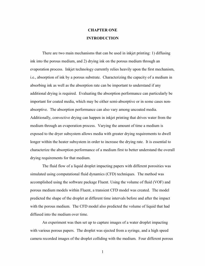
There are two main mechanisms that can be used in inkjet printing: 1) diffusing

ink into the porous medium, and 2) drying ink on the porous medium through an

evaporation process. Inkjet technology currently relies heavily upon the first mechanism,

i.e., absorption of ink by a porous substrate. Characterizing the capacity of a medium in

absorbing ink as well as the absorption rate can be important to understand if any

additional drying is required. Evaluating the absorption performance can particularly be

important for coated media, which may be either semi-absorptive or in some cases non-

absorptive. The absorption performance can also vary among uncoated media.

Additionally, convective drying can happen in inkjet printing that drives water from the

medium through an evaporation process. Varying the amount of time a medium is

exposed to the dryer subsystem allows media with greater drying requirements to dwell

longer within the heater subsystem in order to increase the drying rate. It is essential to

characterize the absorption performance of a medium first to better understand the overall

drying requirements for that medium.

The fluid flow of a liquid droplet impacting papers with different porosities was

simulated using computational fluid dynamics (CFD) techniques. The method was

accomplished using the software package Fluent. Using the volume of fluid (VOF) and

porous medium models within Fluent, a transient CFD model was created. The model

predicted the shape of the droplet at different time intervals before and after the impact

with the porous medium. The CFD model also predicted the volume of liquid that had

diffused into the medium over time.

An experiment was then set up to capture images of a water droplet impacting

with various porous papers. The droplet was ejected from a syringe, and a high speed

camera recorded images of the droplet colliding with the medium. Four different porous

2

media were tested. Three of the media tested were various versions of uncoated plain

paper. The remaining medium was a porous coated medium. The coated medium was

designed to work with an inkjet paper and thus had a highly porous coating layer.

A dimensional analysis was also performed on the droplet/medium interactions.

Using the Buckingham Pi theorem, seven non-dimensional terms were defined. The non-

dimensional terms, along with the experimental data that had been collected, were used to

develop an equation to predict the aspect ratio of the droplet. The results predicted by

both the dimensional analysis and CFD model for the droplet aspect ratio were compared

to experimental data. The results of the computational modeling and dimensional

analysis could be useful to drying applications, such as inkjet printing, where absorption

of a liquid into a porous substrate is critical for drying.

An extensive literary review was conducted and is presented in chapter two of this

thesis. Previous papers looking at how to determine the porosity and permeability of a

medium were studied. Surface tension was also expected to be an important parameter

involved in the droplet/medium interaction. Thus prior work looking at the surface

tension between a liquid and porous substrate was examined, along with previous system

modeling.

After presenting the previous work that was examined, an introduction to the

droplet system under study is presented in chapter three along with a detailed description

of the system geometry. Chapter three also introduces the CFD modeling that was

conducted over the course of the project. The commercial software package, Fluent, was

used to model the system, and thus background information on the models used within

Fluent is given, along with information about the mesh and boundary conditions used.

The approaches used to calculate the required input parameters to the Fluent model are

also given in chapter three. Results from the CFD model are presented. The results

included characterizing the droplet’s geometry after impact, and the volume of water that

has been absorbed by the medium.

3

In addition to the modeling, an experiment was set up to capture images of a

droplet impacting with various media. Chapter four introduces the equipment and

procedure used in the experiment. The various media used in the experiment is also

detailed in chapter six.

The results of the experiment are then presented in chapter five. Details regarding

the procedures used to determine the droplet velocity and contact angle using the camera

images are also presented. Chapter five also compares the experiment results with the

CFD results.

A dimensional analysis of the droplet system was conducted and is presented in

chapter six. Using experimental data and the pi terms calculated from the dimensional

analysis, a correlation to predict the aspect ratio of the droplet after impact was derived.

The uncertainty associated with the aspect ratio correlation is also presented in chapter

six. Details of the procedure used to calculate the uncertainty are presented. The

uncertainties associated with other important parameters are also given in chapter six.

An overall summary of the research project is presented in chapter seven. The

summary highlights the main results of the project. In addition to the summary, a look at

the potential industrial applications of the results is also given, along with a few future

recommendations.

4

CHAPTER TWO

LITERATURE REVIEW

This chapter provides a detailed literary review of technical papers that were

examined over the coarse of this research project. Papers pertaining to the porosity and

permeability of a medium are presented first, followed by papers on the surface tension

between a fluid and porous medium, and finally literature on previous system modeling.

2.1 Porosity and Permeability

The porosity, also known as the void fraction, is defined as the ratio of open

spaces (pores) to the total volume that makes up the medium. The porosity is related to

the permeability, which is the mediums ability to transmit fluid through its pores. There

are various forms of porous media; one such form is a fibrous matte.

There has been a significant amount of experimentation and research on laminar

flow through a fibrous porous medium. Fibrous media are made up of elongated solid

particles. The fiber particles do not necessarily need to be straight and could be randomly

oriented. Plain, uncoated paper could be considered a fibrous medium. It is usually

composed of small cellulose fibers. During the paper making process the fibers become

interlaced, forming a matte of paper.

Jackson and James [1986] gathered and examined significant data related to low

Reynolds number flow through fibrous media. They were able to characterize and

compare the range of experimental data in terms of a dimensionless permeability number

(P), and the solid volume fraction (ф). It was assumed that all fibers were circular and

therefore could be characterized by a single uniform diameter. The data tabulated covers

many types of fiber materials; cellulose was not one of the materials, though.

Nilsson and Stenstorm [1997] looked at the permeability of pulp and paper. They

used the CFD program FICAP to create a model that predicts the permeability of

5

cellulose fiber structures, like those found in paper. The permeability values predicted by

the FICAP model were compared with experimental data. They looked at both structured

and randomly oriented fiber arrangements. Depending on the fiber aspect ratio (Fa), the

calculated permeability values corresponded very well with the experimental data.

Rioux [2003] determined the permeability of various media using experimental

data from a Bristow Absorption Tester. The Bristow tester measured the absorption of a

medium by looking at the amount of liquid volume that is transferred from the tester to

the medium. He was able to calculate the permeability of an uncoated medium using

Darcy’s Law to determine a relationship for permeability based on the measured

penetration depth from the Bristow tester, along with velocity and pressure difference

measurements from a Sheffield-type porosimeter.

Rioux was also able to determine the permeability of a coated medium. A coated

medium’s permeability was calculated based on a relationship using the total liquid

volume (TLV) measured from the Bristow tester along with other important medium

parameters such as porosity, pore radius, and contact angle between the medium and

fluid. The porosity and pore radius of the coating layer was measured using a mercury

porosimeter. A camera was used to capture images of a drop settling on the coated

surface. These images were analyzed to determine the contact angle between the medium

and fluid.

Ergun [1952] studied the flow of a fluid through a packed bed of granular solids.

A packed bed is composed of tiny circular solid particles that are packed tightly together

to form a porous medium. The coating layer of a porous medium could be considered a

packed bed. He determined that the total energy loss, which results in a pressure drop in

the packed bed, can be treated as the sum of viscous and kinetic energy losses. For

laminar flow, the kinetic energy loss terms goes to zero.

Lindsay [1990] studied the anisotropic behavior of paper. Three mutually-

perpendicular directions were typically used to describe paper: the machine direction, the

6

cross-web direction, and the transverse direction. During the paper production process,

the paper is moved through roller presses, and the direction parallel to the flow of

material out of the press is considered the machine direction. The transverse direction

was normal to the sheet/paper, while the machine direction and cross-web direction were

parallel to the sheet, as presented in Figure 1. The machine and cross-web directions are

often referred to as “in-plane” permeability. It is assumed that any differences between

the machine and cross-web direction are very small and can be neglected. Thus the in-

plane permeability is assumed to be isotropic. This should be a valid assumption since

droplets typically spread in a circular fashion when interacting with paper. Any major

differences within the in-plane permeabilities would result in non-circular, or anisotropic,

droplet spreading.

Figure 1: Major Paper Directions

Even though paper is recognized as an anisotropic medium, most permeability

measurements have been focused on the transverse direction. Some previous work has

7

been done though to characterize the differences in permeability between the in-plane and

transverse paper directions. Lindsay [1990] used a hydraulic press to measure the lateral

and transverse permeabilities under uniform loads. He found the anisotropy ratio of in-

plane to transverse permeability to be generally greater than one. Hamlen and Scriven

[1991] found that for an uncompressed sheet, the anisotropy ratio is around 5.5.

2.2 Surface Tension

Surface tension is an important physical parameter for the droplet/porous medium

interaction. After the initial impact the droplet will wick into the capillary spaces and

spread out on the porous medium. De Gennes et al. [2004] determined that the spreading

of the droplet can be characterized by the spreading parameter, S, which is a comparison

between the wet and dry surface energy of the substrate. For a droplet on a substrate

there are three surface tension coefficients involved: the surface tension at the

substrate/air, substrate/liquid, and liquid/air interfaces. The spreading parameter is a

function of all three surface tension coefficients. De Gennes et al. [2004] also showed

that the surface tension can be related to the van der Waals energy. The van der Waals

energies are the result of dispersion forces between molecules. They are the weakest of

the intermolecular forces, but they play an important role in surface interactions.

Rioux [2003] also determined contact angle, and thus surface tension, has a

significant impact of the physical properties of the water droplet as it impacts and

diffuses with the medium. As stated previously, he determined the contact angle through

camera images.

2.3 System Modeling

A significant amount of previous research and modeling has been done on

droplets impacting with a solid surface. Impact with a porous surface is a more

8

complicated phenomenon. It involves not only spreading of the droplet along the surface,

but also absorption into the permeable surface.

There have been considerable studies’ looking at the absorption of a liquid into a

porous medium using the Lucas-Washburn equation, which describes the penetration of a

liquid into a cylindrical capillary. One such study was done by Mamur and Cohen

[1997]. They used the Lucas-Washburn equation to characterize the liquid penetration of

porous media. Another study by Hamraoui and Nylander [2002] used an analytical

approach to model the diffusion of liquid into a porous structure. The model was based

on the Lucas-Washburn equation. These studies neglected inertial effects due to impact

forces though.

Numerical models have been developed to simulate flow of a liquid droplet as it

impacts with a porous medium. One such model was developed by Hsu and Ashgriz

[2004]. Their numerical model simulated a droplet impacting with two parallel plates

separated by a specified distance. This specified gap created a radial capillary that drew

the droplet towards the cap due to a pressure difference between the internal droplet

pressure and the pressure within the gap. The model assumed a free surface condition. A

free surface condition occurs when a fluid boundary interfaces with another fluid. The

effect of the external fluid upon the motion of the internal fluid is considered negligible.

This assumption is valid when the internal fluid has a much larger viscosity and density

in comparison with the external fluid. The model also assumed 2-dimensional,

incompressible, and transient flow. It also took into account the surface tension at the

interface between the liquid and porous substrate. The surface tension was modeled

using the continuum surface force (CSF) model.

The Hsu-Ashgriz model used the hydrodynamics code RIPPLE to solve the

incompressible Navier-Stokes equations for a rectilinear mesh geometry using a finite

difference method. The model used the volume of fluid (VOF) technique to track the

position and shape of the droplet. Results of the model showed that the droplet

9

properties, velocity, contact angle with the substrate, and capillary geometry were

important proprieties related to droplet spreading and absorption.

Reis et al. [2004] also created a numerical model to simulate a liquid droplet

impacting with a porous medium. This model also assumed free surface flow for the

permeable surface. It took into account inertial effects, surface tension inside and outside

the porous medium, pressure at impact, and capillary effects. The model assumed the

fluid flow is governed by the continuity of mass and momentum conservation equations.

These equations were discretized using the finite volume method. This was done using

the SIMPLEC algorithm. Position and geometry of the droplet was tracked using the

marker-particle method.

A numerical model was also created by Alam et al. [2007]. Their model and

research was mainly focused on how an irregular surface affects the spreading and

absorption of an impacting droplet. They did also look at impact with a flat porous

surface though. The CFD software FLOW3D was used to create the model, which used

the VOF method. The geometry was discretized with a rectilinear mesh and used the

finite difference method to solve the Navier-Stokes equations. Values for fluid viscosity,

surface tension, capillary pressure, and medium porosity were all input into the model.

FLOW3D was able to calculate the contact angle between the fluid and porous medium.

Results showed the droplet viscosity, velocity, and pressure outside of the medium to be

important parameters. An irregular porous surface resulted in asymmetrical spreading

and absorption of the liquid, but a flat profile for the surface resulted in an approximately

circular perimeter.

Kannangara et al. [2006] looked at the interactions between a paper surface and a

liquid droplet. They used a high-speed CCD camera study the physics of a drop as it

impacts with sized paper. The sized papers had different levels of solvent content that

made up the cellulose film of the particular paper. Experimental results were compared

with the predicted results based on a model developed by Park et al. [2003]. The model

10

predicted the maximum drop spreading ratio, Dm, which is the ratio of the maximum drop

diameter after impact and the spherical diameter of the drop before impact. The Park et

al. model assumes a solid smooth hydrophobic or hydrophilic surface instead of a porous

interface. Thus, diffusion into the paper does not appear to be accounted for in this

model.

11

CHAPTER THREE

CFD SIMULATION

CFD modeling was used as a simulation tool to predict the absorption

performance of a medium using the Fluent commercial software. The model predicts the

shape and velocity of the droplet at different time intervals. It also predicts the time and

amount of fluid from the droplet that has diffused into the porous substrate. This chapter

describes the CFD model in detail. A detailed description of the system analyzed in this

study is also given.

3.1 System Introduction

In order to better understand the absorption mechanism, a system involving a

droplet coming into contact with a porous medium was analyzed. Traditionally ink has a

high percentage of water content. Thus for the purposes of this project, the droplet was

assumed to be composed of water. The droplet was assumed to be ejected from a nozzle,

for this project a syringe nozzle was used.

Various papers intended for use with an inkjet printer were used as the porous

substrate with which the droplet collides. All of the media were classified as porous,

including the coated medium that was considered. The coated medium was composed of

a base layer, which was made up of many cellulose fibers all packed together.

Surrounding the base layer was a coating layer on each side. The coating layer was

composed of tiny silica particles packed tightly together.

In addition to the coated medium, various uncoated media were also considered.

The uncoated, or plain papers, were composed of cellulose fibers matted together, similar

to the base layer of the coated medium. Various uncoated papers were tested, with each

12

one having a unique porosity and permeability value. The permeability is defined as a

substrates ability to convey fluid through its pores.

3.1.1 System Geometry

The schematic of the system analyzed is shown in Figure 2. A droplet is ejected

from a nozzle, with a diameter of Dpipe. The droplet is ejected with an average velocity

V, a diameter D, and drops a distance H before impacting the medium. After impact the

height h and diameter d are used to characterize the drop geometry after impact.

Figure 2: Flow Diagram of a Droplet Impacting with a Porous Medium

3.2 Mesh Generation

The geometry of the model is shown in Figure 3. The syringe nozzle has a

diameter of 0.5 mm. After being ejected from the nozzle the droplet free falls in the

atmosphere until it contacts with the porous medium. The atmospheric interaction is

13

represented by an air chamber in the model. The porous medium was assumed to have a

flat uniform surface.

Figure 3: Model Geometry

A symmetrical condition was assumed for the nozzle, air chamber, and porous

medium. This reduced the mesh size and computation time. It was also assumed that

after impact the droplet spread along the porous surface in a circular and symmetrical

pattern (i.e. the perimeter of the droplet was approximately a circle). Due to the

symmetry of the resulting circular droplet, which grows parallel to the medium surface,

the droplet was modeled with 2-dimensional analysis. Figure 4 shows a 2-dimensional

mesh plot. It was generated using the commercial software package Gambit. The nozzle

and air chamber of the mesh was composed of 4 node quadrilateral elements that had an

14

edge length of 0.125 mm. The medium section of the mesh was also created with

quadrilateral elements, but with a much smaller edge length depending on the medium.

Mesh independence was verified by refining the mesh and ensuring that the results were

not significantly different. The mesh was refined by reducing the element edge length by

half. This resulted in a 2% change in the resulting droplet geometry, and was not

considered significantly different. The refined mesh significantly increase computation

time, thus the coarser mesh was used.

Figure 4: Typical Mesh Plot

In Fluent, an axisymmetric condition must be mirrored around the x-axis. Thus,

the nozzle velocity and corresponding flow of the droplet were in the x-direction. Using

the camera function in Fluent, the mesh was rotated clockwise by 90°.

3.3 Boundary Conditions

A velocity inlet was specified for the uppermost horizontal line of the model,

while the lowermost horizontal line was specified to be a pressure outlet boundary

15

condition (Figure 2). A pressure outlet boundary condition was also specified along the

vertical lines of the air chamber and medium.

The line between the air chamber and porous medium was specified as an interior

boundary. This represents the boundary between the porous and non-porous fluid zones.

The porous zone represents the porous medium and creates resistance to fluid flow

through the zone.

The remaining lines/boundaries were specified as walls. This created two

different wall conditions: the nozzle wall and the air chamber wall. A contact angle

between the fluid mixture and the walls of the syringe nozzle was defined as 90 degrees,

which represents the contact angle between water and steel. The nozzle was assumed to

be composed of steel.

3.4 Fluent Models

The volume of fluid (VOF) model within Fluent was used to define the droplet

model. The VOF model assumes a multi-flow problem. In this case the two fluids are

water and air. Several options are available within the Fluent VOF model to determine

the droplet’s geometry at the air/water interface. For this model the “Geometric

Reconstruction Scheme” was used. The geometric reconstruction scheme interpolates

near the interface of the two fluids using the piecewise-linear approach shown in Fluent

User’s Guide [2007].

Air was defined as the primary phase with water considered as the secondary

phase. The two phases together are referred to as the fluid mixture. Fluent uses the

continuum surface force (CSF) model for surface tension. The CSF model adds an

additional source term to the momentum equation. This source term represents a pressure

drop across the surface between the two fluids. The pressure drop is a function of the

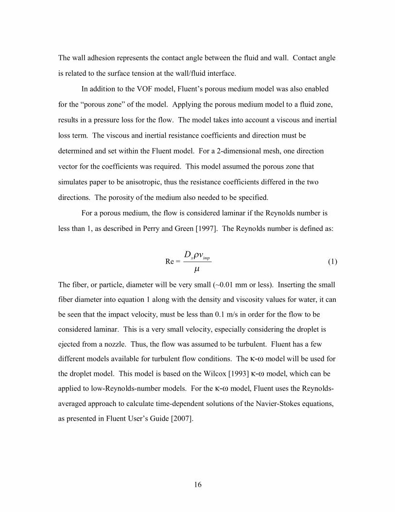
surface tension coefficient. Wall adhesion was also enabled within the Fluent model.

16

The wall adhesion represents the contact angle between the fluid and wall. Contact angle

is related to the surface tension at the wall/fluid interface.

In addition to the VOF model, Fluent’s porous medium model was also enabled

for the “porous zone” of the model. Applying the porous medium model to a fluid zone,

results in a pressure loss for the flow. The model takes into account a viscous and inertial

loss term. The viscous and inertial resistance coefficients and direction must be

determined and set within the Fluent model. For a 2-dimensional mesh, one direction

vector for the coefficients was required. This model assumed the porous zone that

simulates paper to be anisotropic, thus the resistance coefficients differed in the two

directions. The porosity of the medium also needed to be specified.

For a porous medium, the flow is considered laminar if the Reynolds number is

less than 1, as described in Perry and Green [1997]. The Reynolds number is defined as:

Re = µρ impx vD

(1)

The fiber, or particle, diameter will be very small (~0.01 mm or less). Inserting the small

fiber diameter into equation 1 along with the density and viscosity values for water, it can

be seen that the impact velocity, must be less than 0.1 m/s in order for the flow to be

considered laminar. This is a very small velocity, especially considering the droplet is

ejected from a nozzle. Thus, the flow was assumed to be turbulent. Fluent has a few

different models available for turbulent flow conditions. The κ-ω model will be used for

the droplet model. This model is based on the Wilcox [1993] κ-ω model, which can be

applied to low-Reynolds-number models. For the κ-ω model, Fluent uses the Reynolds-

averaged approach to calculate time-dependent solutions of the Navier-Stokes equations,

as presented in Fluent User’s Guide [2007].

17

3.5 Fluent Solver

After defining the model for the droplet, the flow solver with Fluent was used to

numerically solve the model. Fluent has the ability to solve flow problems using either a

pressure or density based solver. Both the pressure and density-based solvers are able to

solve the governing flow equations for a model by discretizing the geometry and

integrating the conservation of mass and momentum equations. The geometry is

discretized using the finite volume approach. The two different flow solvers differ in

how they linearize and solve the discretized equations.

For the droplet model the pressure-based solver was used, as the density-based

solver cannot be used with the VOF model. The pressure-based solver determines the

pressure field for the flow by solving a pressure equation, which was created by

manipulating the governing equations These manipulated governing equations for

continuity and momentum are numerically solved using the project method. The

projection method uses a pressure correction equation to ensure that the velocity field

satisfies the continuity equation. For the droplet model the continuity and momentum

equations were solved sequentially using the segregated algorithm. Second-order

accuracy was specified for the equations since a quadrilateral mesh was used for the

model. This was done by setting the momentum scalar equation to “QUICK” in Fluent’s

solution controls panel. The QUICK scheme is appropriate for quadrilateral meshes.

The pressure interpolation scheme was set to the “PRESTO!” scheme, which is

recommended for flows involving porous medium. For “Pressure-Velocity Coupling”,

the PISO algorithm was used. The PISO algorithm is recommended for all transient flow

calculations. The non-iterative time advancement scheme was used to cut down on

computational time by reducing the iterations performed for each time-step while

preserving the overall accuracy of the results.

The droplet model needs to be solved for different time intervals, and thus the

model was solved as a transient problem. This means that the governing equations had to

be discretized for both time and space. For the droplet model, a fixed time step was

18

specified. During the discretization process, all time dependent equations were integrated

over the fixed time step.

3.6 Input Data

The models within Fluent require a few important parameters to be defined.

Within the VOF model a surface tension coefficient for the porous substrate and fluid

was specified. The methods used to determine the surface tension coefficient and other

input variables described in this section are given in the next section.

The porous medium model within Fluent requires two coefficients to be defined

by the user. Those coefficients are related to the viscous and inertial forces applied by

the fluid. The porous medium model adds an additional source term to the momentum

equations, i.e., the Navier-Stokes equations. This source term creates a momentum sink

that contributes to the pressure gradient within the porous medium. For the case of the

droplet model, the paper will be considered as a homogeneous medium. The source term

(Si) for a homogenous porous medium, as stated in Fluent User’s Guide [2007], is

defined as:

Si = -( )21

2 imi C υρυυαµ

+ (2)

As seen in equation 2, the source term is composed of two parts. The first part accounts

for viscous effects and is represented by Darcy’s equation. The second term accounts for

inertial losses, and the coefficient C2 represents the inertial resistance coefficient.

Another coefficient is defined to account for viscous effects. The viscous resistance

coefficient (VR) is related to the medium’s permeability (α) through the following

equation:

α1

=VR (3)

In addition to the porous medium and VOF model, an impulse velocity was

applied at the nozzle inlet. The velocity was applied for specified time duration. When

19

modeling turbulent flow in Fluent, both the κ and ω values at any inlet boundary must be

defined. For the droplet model there is only one inlet boundary condition, which is at the

nozzle inlet.

3.7 Property Calculations

The important properties associated with the droplet system needed to be defined

within the Fluent model. These properties included porosity, permeability, and surface

tension.

3.7.1 Porosity and Permeability

The permeability, and thus the viscous resistance coefficient, was determined

based on the fibrous and packed bed models. Tabulated experimental data for a cellulose

fibrous matte was used to determine the permeability of uncoated medium. The

experimental data was based on the work Nilsson and Stenstorm [1997], which compared

the solid void fraction to the dimensionless permeability of the medium. The

dimensionless permeability is defined by the following equation:

P = 2aα

(4)

Tabulated results for their experimental data of a random fiber arrangement are shown in

Table 1.

Table 1: Tabulated Permeability Data for Cellulose Fibers by Nilsson and Stenstorm

[1997]

ф P

0.3 0.0195

0.4 0.00633

0.5 0.00109

20

Figure 5 plots the data in Table 1 in order to create a best fit equation that was used to

determine a media dimensionless permeability based on its solid void fraction. An

exponential trend-line provided the best fit curve fit for the data points.

Plot of Tabulated Permeability Data of Cellulose

y = 1.64e-14.421x

0

0.005

0.01

0.015

0.02

0.025

0 0.1 0.2 0.3 0.4 0.5 0.6

Solid Void Fraction

Dim

ensi

onle

ss P

erm

eabi

lity

[P/a

^2]

Figure 5: Plot of Tabulated Cellulose Permeability Data

The fiber diameter for a medium was measured using a high magnification microscope.

The total solid fraction for a medium can be defined by the following equation:

smLGρ

φ = (5)

Dry cellulose is considered to have a density of 1.61 g/cm3 based on the work of

Campbell [1947]. It is important to note that cellulose fibers can also absorb water

themselves, but for this study it was assumed that the basis weight was measured for

21

“dry” sheets. The basis weight is usually specified on the ream label, and in general

water accounts for 3-6% of the basis weight.

An alternative to using the basis weight is to use the dry weight of the medium to

calculate the solid fraction.

ssm

dry

ALW

ρφ = (6)

The dry weight of the sample was measured with a moisture balance, which is a scale

with a heat controlled surface. A sample was placed on the scale and then heated until

most of the water had been evaporated from the medium. As the water evaporated the

weight of the medium and scale continued to change with time until most of the water

had evaporated off when the weight of the medium reached steady state. The weight

reported by the scale at steady state was used as the dry weight. Overall thickness of the

medium was measured with the help of a microscope.

Either equation 5 or 6 can be used to calculate the solid volume fraction for the

medium. Equation 6 should be more accurate since it ensures that all moisture has been

removed from the medium, and it was used for un-coated plain paper. Once the solid

fraction was calculated it was compared with previous experimental data to determine the

appropriate dimensionless permeability number. The dimensionless permeability and

measured fiber diameter along with equation 4 to determine the medium’s permeability.

Coated paper typically has two distinct porous layers: the base and the coating

layer. The solid fraction has to be calculated separately for each layer. Since it would be

quite difficult to physically separate the layers and determine the dry weight using the

moisture balance, equation 5 was used to calculate the solid fraction for coated media.

The base layer of a coated medium is typically composed of cellulose fiber, like

those found in plain paper, but the coated layer is usually composed of tiny

pigment/polymer particles. The medium is commonly coated on two sides, with the base

22

layer sandwiched between the coating layers. Inkjet media require a porous coating layer

that can absorb the ink. For these media, the coating layer is commonly composed of a

silica base. In general, the silica particles have a diameter of ~ 0.1 μm.

A microscope was used to determine the thickness of the coating layer. The

overall thickness of the coated medium was also measured and used to determine the base

layer thickness. The coating thickness is calculated by subtracting the thickness of the

base layer from the total thickness and then dividing by the number of coating layers, n.

nLLL Bm

C

−= (7)

The fibrous matte method used for determining the permeability of an uncoated medium

was also applied to the base layer of a coated medium.

The void fraction and solid fraction are related to each other through the

following relationship:

ε = 1 – ф (8)

Once the void fraction of the coating layer was determined, the permeability of the

coating layer was determined using relationships derived for a packed bed.

From Ergun’s [1952] work with packed beds, the permeability and inertial

resistance coefficient can be defined as the equations given in Fluent user’s guide [2007]:

2

32

)1(150 εε

α−

= xD(9)

32

)1(5.3ε

ε

xDC −

= (10)

Once the permeability of the coated or uncoated medium was determined, equation 3 was

used to calculate the viscous inertial coefficient of the medium, and inputted into Fluent’s

porous medium model. The porosity, or void fraction, was also required to be specified

within the porous substrate model.

23

For turbulent flow within the porous region, both the viscous and inertial

resistance coefficients must be defined. Equation 10 was used to determine the inertial

resistance coefficient for a coated medium. For an uncoated medium, the inertial

resistance coefficient can be found using the equations for flow through a perforated plate

with an adjusted loss factor, KL’, which is described in Fluent user’s guide [2007]. An

inertial resistance coefficient, C2, for the plate is defined as:2

2

1

=

εm

L

LKC (11)`

The procedure that was used to arrive at this equation is shown in Appendix A. Equation

11 was used to determine the inertial resistance coefficient for an uncoated medium. The

loss factor at the inlet of the porous region can be treated as a sharp-edged entrance. For

flow at a sharp-edged inlet, the loss factor is 0.5 as stated by Young et al. [1997].

3.7.2 Anisotropic Permeability

Within Fluent’s porous medium model the permeability of the medium can be

specified for 2-3 different directions. The transverse direction is referred to as direction-1

within the porous model, while the in-plane direction is referred to as direction-2, as

shown in Figure 6.

24

Figure 6: Permeability Direction Vectors in Fluent Model

For the 2-dimensional droplet model, both the in-plane and transverse

permeabilities are specified. Based on the work of Hamlen and Scriven [1991], an

anisotropic ratio of 5.5 was used to determine the in-plane permeability based upon the

calculated transverse permeability.

3.7.3 Surface Tension

The surface tension was set with the VOF model. For the droplet system the three

surface tension coefficients can be related to the contact angle between the substrate and

droplet through the Young-Dupre relation given by De Gennes et al. [2004]:

SLSALA σσθσ −=cos (12)

For the droplet model the important surface tension coefficient is the substrate/liquid

interface. This is the surface tension that was specified within the VOF model. The

surface tension coefficient of the liquid/air interface can be determined from tabulated

data for air and water. As mentioned previously, surface tension can be related to the

25

Van der Waals energy as shown by De Gennes et al. [2004]. Using this relationship, the

following equation was derived for the surface tension at the substrate/air interface:

(13)

The derivation of equation 13 is shown in Appendix B. Substituting equation 13 into

equation 12, results in the following relationship:( )

θσθσ

σ cos4

1cos 2

LALA

SL −+

= (14)

This was the equation used to compute the surface tension coefficient between the water

droplet and porous medium.

3.8 Droplet Velocity

In the CFD model the droplet is subjected to an initial velocity, vo, from the flow

out of the syringe. After ejection from syringe, the droplet accelerates due to gravity. In

order to match the desired droplet velocity at impact, the initial velocity of the droplet at

the syringe was calculated based on the impact velocity from the experimental data and

the following equation given by Meriam and Kraige [1997]:

dgimpo tavv −= (15)

The calculated initial velocity was applied at the syringe inlet of the CFD model

The κ and ω values at the velocity inlet also had to be defined. These values were

determined based on the following relationships stated in the Fluent User’s Guide [2007]:

( )2

23 Ivo=κ (16)

l4/1

2/1

09.0κ

ω = (17)

The velocity of the fluid was known at the nozzle inlet and corresponded to the initial

velocity, ov . The turbulence intensity and length scale were calculated based upon the

following equations presented in Fluent user’s guide [2007]:

( )4

1cos 2+=

θσσ LASA

26

( ) 8/1Re16.0 −=I (18)

L07.0=l (19)

For the nozzle inlet, L is equal to the diameter of the nozzle. Thus substituting the nozzle diameter, pipeD , into equation 19 results in the following equation for the turbulence

length scale:

pipeD07.0=l (20)

The Reynolds number for flow at the nozzle inlet can determined from the following

equation:

µρ pipeoDv.Re = (21)

Using the equations defined above, the turbulent kinetic energy and length scale were

calculated and inputted into the Fluent droplet model. Fluent automatically calculates the

values of κ and ω at any non-inlet boundaries.

3.9 Media

Four different media were tested. These media and their associated properties are

listed in Table 2. Media M1 was the only coated media tested. It was composed of two

coated layers with a base layer in between. The coating layers are identical and are

referred to as M1a, while the properties of the base layer were identified as M1b.

Uncoated plain papers made up the remaining media: M2, M3, and M4. Each of the

uncoated media had a unique porosity, permeability, and other material property values.

27

Table 2: Media Set

VR [1/m^2]

Media Name

G [g/m2]

Lm [mm] Ф ε

Dx [mm]

σSL

[dyn/cm]C2

[1/m]α

[m^2]Direction-

1Direction-

2

M1a 15 0.0271 0.2083 0.7917 0.0010 2.56 1468745.33 7.63E-14 1.31E+13 2.38E+12

M1b 151 0.1361 0.6889 0.3111 0.0087 NA 37937.86 6.00E-15 1.67E+14 3.03E+13

M2 75 0.1277 0.4151 0.5849 0.0125 11.42 11441.56 6.46E-13 1.55E+12 2.81E+11

M3 75 0.1201 0.3769 0.6231 0.0104 7.04 10726.10 7.80E-13 1.28E+12 2.33E+11

M4 105 0.1430 0.4390 0.5610 0.0093 9.01 11107.67 2.50E-13 4.00E+12 7.27E+11

3.10 CFD Results

Results of the CFD modeling are presented in this chapter. The analysis and

procedure for determining the input parameters for the model are also presented.

3.10.1 Volume of Water within Media

The “Volume Integrals” function within Fluent was used to calculate the total

volume of water within the porous medium zone. The volume integrals feature integrates

over the specified cell or zone to determine the volume in that region. This was a useful

feature within the CFD model that allowed the absorption of water by the medium to be

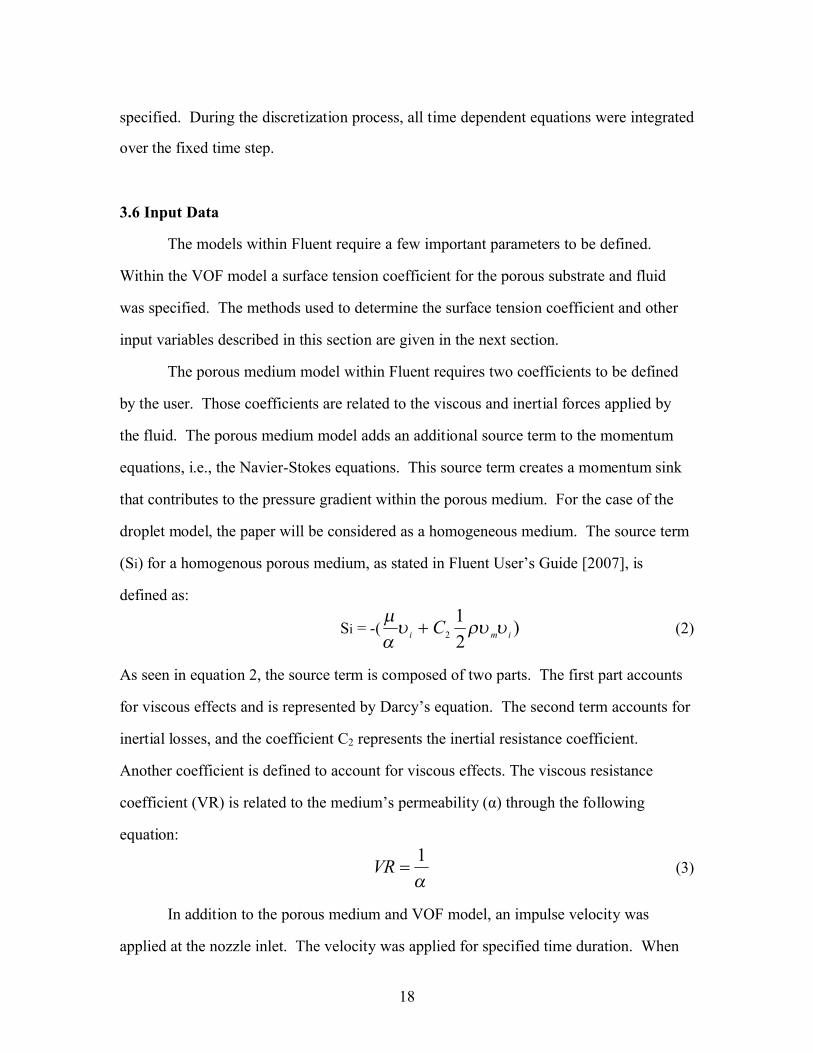
tracked over time. Figure 7 shows the volume of water absorbed into three different

uncoated media, specified as M2, M3, and M4, at various time intervals.

28

Volume of Water Absorbed into MediaUncoated Media

0.0000E+00

5.0000E-10

1.0000E-09

1.5000E-09

2.0000E-09

2.5000E-09

0.05 0.15 0.25 0.35 0.45 0.55 0.65 0.75 0.85 0.95 1.05

Time [sec]

Volu

me

of W

ater

[m^3

]

M2M3M4Log. (M3)Log. (M4)Log. (M2)

Figure 7: Volume of Water Absorbed from the CFD Model for Uncoated Media

The volume of water absorbed into the coated medium, specified as M1, was also

plotted (Figure 8). The model was run for two different meshes: one mesh incorporated

only the top coating layer (1-layer), and the other had three different layers made up of a

base layer surrounded by two coating layers (3-layer). It shows that the 1-layer

model/mesh results seem more reasonable since the 3-layer model has very little water

absorption, which was an unexpected behavior since the coated medium considered was a

porous coated medium that was known to be very absorptive. Also the results from the

1-layer model followed the same trend as the volume of water results for the uncoated

models. This indicates that there were missing parameters or incorrect interface

boundaries defined for the 3-layer model.

29

Volume of Water Absorbed into MediaCoated Media

-1.0000E-10

0.0000E+00

1.0000E-10

2.0000E-10

3.0000E-10

4.0000E-10

5.0000E-10

6.0000E-10

7.0000E-10

8.0000E-10

0.05 0.15 0.25 0.35 0.45 0.55 0.65 0.75 0.85 0.95 1.05

Time [sec]

Volu

me

of W

ater

[m^3

]

M1 - 1 LayerM1 - 3 LayersLog. (M1 - 1 Layer)Log. (M1 - 3 Layers)

Figure 8: Volume of Water Absorbed from the CFD Model for Coated Media

3.10.2 Aspect Ratio

The resulting droplet shape after impact was characterized at various time

intervals as the aspect ratio between the measured diameter and droplet height. The

aspect ratio, r, was defined by the following relationship:

hdr = (22)

Figure 9 shows the resulting CFD aspect ratio for three uncoated media. The

three media had different porosity, permabilities, and surface tension coefficients. All

media had around the same drop velocity of 0.27 – 0.28 m/s

30

CFD Aspect RatioUncoated Media

1.50

2.00

2.50

3.00

3.50

4.00

0.05 0.15 0.25 0.35 0.45 0.55 0.65 0.75 0.85 0.95 1.05

Time [sec]

aspe

ct ra

tio (r

) M2M3M4Log. (M3)Log. (M4)Log. (M2)

Figure 9: CFD Aspect Ratio for Uncoated Media

The coated medium was modeled with two different meshes: one with only 1-

layer, the top coated layer, and another with 3-layers, which had two coated layers and a

base layer. Results for the aspect ratio from the two different meshes are shown in Figure

10.

CFD Aspect RatioCoated Media

5.20

5.30

5.40

5.50

5.60

5.70

5.80

5.90

6.00

6.10

6.20

6.30

0.05 0.15 0.25 0.35 0.45 0.55 0.65 0.75 0.85 0.95 1.05

Time [sec]

aspe

ct ra

tio (r

)

M1 - 1 LayerM1 - 3 LayersLog. (M1 - 1 Layer)Log. (M1 - 3 Layers)

Figure 10: CFD Aspect Ratio for Coated Media

31

CHAPTER FOUR

EXPERIMENTAL TEST FACILITY

An experiment was set up with a high speed camera to capture images of a water

droplet impacting with various porous media. The details of the equipment and

procedure of the experiment are given in this chapter.

4.1 Experimental Schematic

Figure 11 shows a schematic of the experimental setup. The setup included a

syringe that ejected a droplet onto a medium. The syringe and medium are attached to a

common fixture. A high magnification scope lens was focused upon the syringe nozzle

and medium. The lens was attached to a high speed camera. Figure 12 shows a picture

of the fixture, nozzle, lens, and medium (paper). A computer attached to the camera

recorded the video images of the droplet as it was ejected from the nozzle and impacted

with the medium.

32

Figure 11: Experimental Schematic

Figure 12: Close Up View of Syringe/Lens Setup

33

4.2 Syringe

A syringe filled with de-ionized water was used to eject a water droplet. The

syringe had a volume 10 mL. Attached to the end of the syringe was a nozzle with an

inner diameter of 0.5 mm. The syringe was able to produce a single water droplet by

temporarily compressing the syringe plunger by hand.

4.3 Fixture

A fixture was used to position both the medium and syringe. The fixture was

composed of a number of aluminum brackets. Using the brackets, the syringe was fixture

such that the nozzle was perpendicular to the medium. The fixture was adjustable in the

vertical direction and allowed the distance between syringe nozzle and medium to be

adjusted. For the experiment the fixture was set to provide a 10 mm gap between the tip

of the nozzle and the top of the medium.

4.4 Camera and Lens

A high speed camera was a scope lens was used to record the droplet formation,

ejection, and impact with the medium. The scope lens was able to fit into small spaces.

For the experiment the lens was taped down to the fixture, and was able to provide a view

of the end of the nozzle and medium, as shown in Figure 12. The camera was set to

capture 400 frames per second, and the resulting video was saved at a playback rate of 1

frame per second. A total of 5.1 seconds of real time data was captured.

4.5 Other Equipment

A moisture balance was used in order to calculate the solid fraction, and thus

porosity of the media tested. The metal balance heats a sample up while in parallel

measuring the weight of the sample. The resulting dry weight, Wdry, was used in

34

conjunction with equation 6 to determine the solid fraction of the medium. Samples of

each of the uncoated media were tested. Each sample was a 60 by 60 mm square.

A microscope was used to measure the overall medium thickness, and for the

uncoated media this was also used to measure the fiber diameter. The microscope had a

camera attached, and a still image was captured for each measurement. Figure 13 shows

a typical image used for measuring the overall medium thickness. For each medium, five

different measurements were taken, and the average of those measurements was used as

the overall medium thickness. The coating thickness was measured using the same

procedure. Figure 14 shows one of the images used to determine coating thickness.

Figure 13: Media Thickness Image of M2

35

Figure 14: Coating Thickness Image of M1

Microscope images were also used to measure the fiber diameters of the uncoated

media. Again five different measurements were taken for each medium, and the average

was used as the fiber diameter of the medium. Figure 15 shows an example of a

microscope measurement for fiber diameter.

36

Figure 15: Fiber Diameter Image for M2

4.6 Test Procedure

Water droplets impacting with various coated and uncoated papers were recorded

with the high speed video camera. For each paper/medium, a sample was placed on a flat

surface provided by the fixture. The syringe was then used to produce a water droplet

that impacts with the medium. A high speed camera with a scope lens was used to record

the droplet during ejection and impact with the paper. The camera captured video and

still images of the droplet. These images were then analyzed to determine the droplet

velocity and shape after it impacts with the medium.

This test procedure was repeated across the various media. The droplet volume

and velocity were also varied across different experimental runs.

37

CHAPTER FIVE

EXPERIMENTAL RESULT AND COMPARISIONS

Results from the experiment are presented in this chapter. The results for the

aspect ratio are also compared with results from the CFD model.

5.1 Calculated Properties

The images and video from the high speed camera was used to calculate

properties associated with the droplet/medium system. These properties included the

contact angle and average velocity.

5.1.1 Contact Angle

The contact angle between the medium and water was measured from video

images. Immediately after impact the droplet experiences an oscillating motion. Once

this oscillation had dampened out, the contact angle was measured. The droplet was for

the most part static at this point. Figure 16 shows a typical image of the contact angle.

Four different measurements were taken for each medium, and the average of these four

measurements used as the contact angle. Table 3 lists the resulting contact angle for each

medium. The contact angle was then used, along with equation 14, to determine the

surface tension coefficient between the medium and water droplet.

Figure 16: Contact Angle Image for M2

38

Table 3: Average Contact Angle

5.1.2 Average and Impact Velocity

Images from the high speed camera were analyzed to determine both the average

and impact velocity of the droplet. The average velocity (V) was determined by

measuring the total height (H) the droplet has fallen and the time it took to fall ( dt ), as

shown in equation 23. The average velocity varied between runs in the range of 0.25 –

0.36 m/s.

dtHV = (23)

A second velocity measurement was also taken to determine the impact velocity ( impv ), which corresponds to the droplet’s velocity right before impact with the medium.

As the droplet approached a height of 2 mm above the medium, the exact distance

between the droplet and medium was measured using the high speed camera images.

This distance was specified as H’. The time it took the droplet to fall from H’ to contact

with the medium was also measured and recorded as 'dt . The following equation was

then used to calculate the impact velocity, which varied from 0.25 - 0.42 m/s:

''

dimp t

Hv = (24)

For most of the experimental runs the initial droplet velocity out of the syringe

was very small. The total height the drop had to fall, H, was also very small (~10 mm).

Thus for cases with a small initial velocity, the impact velocity was approximately equal

Media

Contact Angle

[degrees]M1a 51.5M2 78.25M3 68M4 73

39

to the average velocity. For a few cases, though, this was not the case, and the measured

impact velocity was significantly higher than the average velocity measurement. Thus,

the initial velocity out of the syringe was not negligible in these cases.

5.2 Aspect Ratio

The high speed camera images were also used to characterize the droplet shape

after impacting with the porous medium. The droplet shape was characterized at various

time intervals with the aspect ratio between the measured diameter and droplet height

(Equation 22).

5.3 Data Comparisons

The aspect ratios from the CFD model were compared with those from the

experimental data. The CFD versus experimental aspect ratio was plotted for each

medium at a drop velocity around 0.27 - 0.28 m/s (Figures 17-20). It should be noted that

the axes on the figures below do not start at zero.

Aspect Ratio ComparisonCoated Media - M1

V = 0.28 m/s

5.00

5.20

5.40

5.60

5.80

6.00

6.20

6.40

6.60

0.05 0.15 0.25 0.35 0.45 0.55 0.65 0.75 0.85 0.95 1.05

Time [sec]

aspe

ct ra

tio (r

)

CFD - 1 LayerExperimentalLog. (CFD - 1 Layer)Log. (Experimental)

Figure 17: Aspect Ratio Comparison of M1

40

Aspect Ratio ComparisonUncoated Media - M2

V = 0.27 m/s

1.50

1.60

1.70

1.80

1.90

2.00

2.10

2.20

2.30

2.40

2.50

0.05 0.15 0.25 0.35 0.45 0.55 0.65 0.75 0.85 0.95 1.05

Time [sec]

aspe

ct ra

tio (r

)

CFDExperimentalLog. (Experimental)Log. (CFD)

Figure 18: Aspect Ratio Comparison of M2

Aspect Ratio ComparisonUncoated Media - M3

V = 0.27 m/s

2.50

2.70

2.90

3.10

3.30

3.50

3.70

3.90

0.05 0.15 0.25 0.35 0.45 0.55 0.65 0.75 0.85 0.95 1.05

Time [sec]

aspe

ct ra

tio (r

)

CFDExperimentalLog. (CFD)Log. (Experimental)

Figure 19: Aspect Ratio Comparison of M3

41

Aspect Ratio ComparisonUncoated Media - M4

V = 0.28 m/s

2.50

2.55

2.60

2.65

2.70

2.75

2.80

2.85

0.05 0.15 0.25 0.35 0.45 0.55 0.65 0.75 0.85 0.95 1.05

Time [sec]

aspe

ct ra

tio (r

)

CFDExperimentalLog. (Experimental)Log. (CFD)

Figure 20: Aspect Ratio Comparison of M4

For each experimental run, a corresponding CFD model was also run. The aspect

ratio was compared between each experimental and CFD run, and the associated

deviation between the two was calculated. Figures 21 and 22 below show the percent

deviation between the model and experiment aspect ratios. The following equation was

used to calculate the percent deviation:

−=

EXP

EXPCFD

rrrDeviation 100% (25)

42

Percent Deviation Between CFD Model and Experiment Aspect RatiosData Points at Time < 0.1 Seconds after Impact

-100.00%

0.00%

100.00%

200.00%

300.00%

400.00%

500.00%

Dev

iatio

n (%

)

M1M2M3M4

Figure 21: CFD Model Aspect Ratio Deviation < 0.1 Seconds after Impact

Percent Deviation Between CFD Model and Experiment Aspect RatiosData Points at Time ≥ 0.1 Seconds after Impact

-25.00%

-20.00%

-15.00%

-10.00%

-5.00%

0.00%

5.00%

10.00%

15.00%

20.00%

25.00%

Dev

iatio

n (%

)

M1M2M3M4

Figure 22: CFD Model Aspect Ratio Deviation ≥ 0.1 Seconds after Impact

The two figures above show that after a certain time, about 0.1 seconds after

impact, the CFD model has an error range of +/- 20%. Yet the error associated with the

predicted aspect ratio by the model increases significantly at times before 0.1 seconds.

Images from the high speed camera show that immediately after impact, around 0.01

43

seconds, the droplet oscillates (Figures 24, 26, & 28). The CFD model lacks this

oscillation effect (Figures 23, 25, & 27). By 0.1 seconds, the oscillation has subsided and

the model more closely corresponds to the experimental results (Figures 29 & 30).

Figure 23: CFD at 0.005 sec. Figure 24: Experiment at 0.005 sec.

Figure 25: CFD at 0.01 sec. Figure 26: Experiment at 0.01 sec.

44

Figure 27: CFD at 0.02 sec. Figure 28: Experiment at 0.02 sec.

Figure 29: CFD at 0.1 sec. Figure 30: Experiment at 0.1 sec.

The results indicate that the porous medium model within Fluent is not able to

account for all of the inertial effects that occur immediately after impact. It appears that

the base porous model within Fluent is not able to account for all on the inertial forces

produced at impact. The model does not treat the porous zone as a solid surface, but

instead considers it another fluid zone that will have a pressure drop across it due to the

porous zone. This could be a contributing factor to the lack of droplet oscillation

immediately after impact. Thus the CFD model should only be used to predict the

relative droplet geometry at a time interval greater than or equal to 0.1 seconds after

impact.

45

CHAPTER SIX

DIMENSIONAL AND UNCERTAINTY ANALYSIS

A dimensional analysis was performed for the droplet/medium system. The

analysis and results are presented in this chapter. An uncertainty analysis was also

performed to determine the uncertainty associated with the parameters used in the CFD

model and dimensional analysis. The procedure used to estimate uncertainty, along with

the results is presented.

6.1 Dimensional Analysis

A dimensional analysis can be performed to help understand the physical

parameters of a system and their relationship. The analysis produces a set of

dimensionless equations that describe the important variables of the system. Since the

equations are dimensionless they are independent of the system units, and thus could be

applied to other systems. This also means that the dimensionless parameters are scalable.

An application of the scalable feature would be to create a much smaller model of a

system within a laboratory, where experimentation could easily occur. Any modeling of

the system with non-dimensional variables could be applied to much large systems

outside of the laboratory. This is an example of how a dimensional analysis can be used

as an effective tool in understanding a system of variables.

The droplet system shown in figure 2 was subjected to a dimensional analysis.

The Buckingham Pi theorem was used to determine the important non-dimensional terms

required to describe the system. Using the non-dimensional variables, along with

experimentation data, a function for the droplet’s aspect ratio was derived. The

dimensional analysis and results are presented in the next two sections.

46

6.1.1 Derive Pi Terms

A non dimensional analysis was performed for the droplet-medium interaction.

Ten independent parameters were identified to be the important variables for the system

under study through the following relationship:

f(h,d,H,D,V,ρ,μ,σ,ε,t) = 0 (26)

These variables consist of three basic dimensions; mass (M), length (L), and time

(T). Upon inspection, three different repeating variables were identified. These three

variables were: D, V, μ.

With ten total variables and three repeating variables, seven non dimensional pi

terms are required for the droplet system. These pi terms were calculated and these

calculations can be found in Appendix C. The resulting pi terms are list below:

Dh

=1π (27)

hd

=2π (28)

DH

=3π (29)

Re4 ==µ

ρπ VD (30)

WeDV==

σρ

π2

5 (31)

επ =6 (32)

τπ ==HtV

7 (33)

The fourth pi term resulted in the Reynolds number (Re), while the fifth pi term resulted

in the Weber number (We). Also the second pi term was equal to the aspect ratio, r.

6.1.2 Aspect Ratio Correlation

Once the pi terms for the droplet system had been identified, they were calculated

using the experimentation data. These pi terms were calculated for various media, drop

velocities, drop volumes, and time intervals. Each medium had a different porosity, or

47

void fraction, along with a different surface tension between the medium and fluid.

Figures 31 and 32 show some of the results.

Experimental Dataπ2 vs. π7

2.00

2.50

3.00

3.50

4.00

4.50

5.00

5.50

6.00

6.50

7.00

0.00 10.00 20.00 30.00 40.00 50.00

π7

π2

We=0.25,ε=0.31,Re=862,π3=1.96We=0.31,ε=0.56,Re=1003,π3=1.75We=0.37, ε=0.62,Re=950,π3=950

We=1.11,ε=0.79,Re=1013,π3=1013Power (We=1.11,ε=0.79,Re=1013,π3=1013)Power (We=0.37,ε=0.62,Re=950,π3=950)Power (We=0.31,ε=0.56,Re=1003,π3=1.75)Power (We=0.25,ε=0.31,Re=862,π3=1.96)

Figure 31: π2 versus π7 for Various Weber Numbers and Porosities

Experimental Dataπ2 vs. π7Media M2

1.25

1.45

1.65

1.85

2.05

2.25

2.45

2.65

2.85

0.00 10.00 20.00 30.00 40.00 50.00

π7

π2

Re=613,We=0.20,π3=4.92Re=694,We=0.16,π3=2.88Re=851,We=0.22,π3=2.5Re=862,We=0.19,π3=1.96Re=1056,We=0.23,π3=1.35Power (Re=1056,We=0.23,π3=1.35)Power (Re=862,We=0.19,π3=1.96)Power (Re=694,We=0.16,π3=2.88)Power (Re=851,We=0.22,π3=2.5)Power (Re=613,We=0.20,π3=4.92)

Figure 32: π2 versus π7 for Various Reynolds Numbers

48

Figure 31 shows that as the surface tension between the fluid and medium

decreases, the droplet aspect ratio increases. The aspect ratio also increased as the

porosity increased. There was also a small increase in the droplet aspect ratio over time.

For most cases as the Reynolds number increased, the aspect ratio also increases, as

shown in Figure 32. Not all cases fit this trend, though, and it should be noted that the

drop volume was different between each run. The highest drop volume corresponded to

the lowest aspect ratio. Thus the variation in drop volume may contribute to the

deviations in a clear trend between the Reynolds number and aspect ratio.

Since the entire seven pi terms were varied across the different experimental runs

and medium combinations, a relationship was derived between the aspect ratio, π2, and

the remaining six pi terms. It was assumed that the aspect ratio was a function of the

remaining pi terms, as shown in the equation below. 7

76

65

54

43

31

12aaaaaaC πππππππ = (34)

A system equation was developed by rearranging equation 34 such that one side

of the equation was equal to zero. The resulting system equation, if , is shown below.

12

77

66

55

44

33

11 −=

πππππππ aaaaaa

iC

f =0 (35)

The pi terms calculated for each experimental run were used to develop a set of

system equations. Using the “Solver” feature within Excel, the unknown coefficients

were then determined based on the set of system equations. The Solver feature was set

up to minimize the sum of the squares of the system equations. The sum of the squares is

defined by the following relationship:

∑=

−

m

ii ff

1

2_

(36)

The mean value, f , was zero for the system equation, as defined by equation 35.

Excel’s Solver feature determined the coefficient values that would minimize the sum of

49

the squares of the system equations based on the experimental data. Appendix D shows

the Solver worksheet. The resulting equation is shown below:0277.0

70302.0

60506.0

51395.0

40861.0

356.1

12 328.0 −−−−= πππππππ (37)

Equation 37 has a percent deviation of +/- 10% from the experimental aspect ratio

for data points at a time greater than or equal to 0.1 seconds after impact (Figure 33).

The standard deviation for the range is 2.72%. The equation is only valid for the

following parameter intervals:

45.4387.379.031.0

11.116.01056Re613

≤≤≤≤

≤≤≤≤

τεWe

% Deviation Aspect Ratio Correlation from Experimental Data

-10.00%-8.00%

-6.00%-4.00%-2.00%0.00%

2.00%4.00%6.00%

8.00%10.00%

Dev

iatio

n (%

)

M1M2M3M4

Figure 33: Percent Deviation of Aspect Ratio Correlation

6.2 Uncertainty Analysis

The uncertainty analysis was carried out to calculate the uncertainty associated

with the aspect ratio correlation. The uncertainty was also calculated for all major input

parameters into the CFD model.

Equation 37 for the aspect ratio has seven parameters associated with it, as shown

below:

50

0277.01395.00584.056.1

0302.00506.00106.00889.0735.1

2 328.0tHh

VDµ

εσρπ = (38)

The uncertainty associated with the aspect ratio equation, U 2π , was calculated using the

following relationship:

∂∂+

∂∂+

∂∂+

∂∂+

∂∂=

2

2

2

2

2

2

2

2

2

2

22

1 εεπσ

σππρ

ρππ

ππ εσρ UUVU

VUDU

DU VD

21

2

2

2

2

2

2

2

2

∂∂

+

∂∂

+

∂∂

+

∂∂

+ tUt

UHUH

hUh tHh

πµ

µπππ

µ (39)

Similar relationships were used to estimate the uncertainty of other calculated

parameters such as porosity, surface tension, permeability, and inertial resistance. There

were numerous equations, similar in form to equation 39, involved in the uncertainty

analysis. In order to deal with all of the uncertainty equations, an Excel macro was

written. The Excel macro and full uncertainty calculations are shown in Appendix E.

The coated and uncoated media had different porosities associated with them,

based on the packed bed and fibrous matte models. Thus the calculated uncertainty for

aspect ratio was also different between the coated and uncoated media. The coated and

uncoated medium uncertainties were calculated assuming a packed bed and fibrous matte

model respectively.

6.2.1 Uncertainty Results

A summary of the calculated uncertainties for all parameters associated with the

aspect ratio and CFD model are listed in Table 4. These results were calculated using the

procedure presented in the previous section.

51

Table 4: Estimated Uncertainty of Parameters

ParameterUncertainty Estimates

Length +/- 0.1%Time +/- 0.1%

Density +/-0.5%Viscosity +/-0.5%Velocity +/-0.16%

Surface Tension +/-1.9%Void Fraction/Porosity +/-1.3%

Paper GSM +/-0.25%Media Sample Dry Weight +/-0.4%Coated Particle Diameter +/-1%

Dimensionless Permeability +/-2%Uncoated Droplet Aspect Ratio (π2) +/-10.1%Coated Droplet Aspect Ratio (π2) +/-20.5%

Uncoated Permeability (Viscous Coefficient) +/-2.0%Coated Permeability (Viscous Coefficient) +/-4.8%

Uncoated Inertial Resistance +/-3.3%Coated Inertial Resistance +/-3.0%

52

CHAPTER SEVEN

SUMMARY AND CONCLUSIONS

The project presented in this thesis took an in depth look into a droplet impacting

with a porous medium. The resulting geometry of the droplet after impact was studied

and characterized by the droplet aspect ratio. An experiment was set up to study a water

droplet impacting with porous papers. Four different media were examined, with one

being a porous coated medium and the remaining three composed of un-coated plain

paper. A high speed camera captured the water droplet as it was ejected from a syringe

nozzle and then collided with the medium. The camera images were analyzed to

determine the droplet volume, velocity, and aspect ratio.

In addition to the dimensional analysis the system was modeled using the CFD

software Fluent. Using the VOF and porous medium models within Fluent a model

simulating the droplet system was created. The model was run to simulate the

experimental data. The CFD results were then compared to the experimental results for

aspect ratio. It was determined that the CFD model was unreliable immediately after

impact until 0.1 seconds after impact. After this time the CFD model was able to predict

the droplet aspect ratio within a range of +/- 20% compared to the experimental data.

The CFD model could be further improved by trying to understand the errors associated

with droplet immediately after impact. Most likely an additional term/function needs to

be added to incorporate the droplet oscillation effect immediately after impact. This

additional functionality would account for inertial effects caused by impact.

Both the CFD model and experimental results showed that the porous coated

medium had the highest aspect ratio. This medium also had the highest porosity value,

and lowest surface tension coefficient between the medium and water droplet.

53

A dimensional analysis was also performed for the droplet system. The resulting

pi terms were used along with the experimental data to derive an equation to predict the

aspect ratio. The resulting equation was able to predict the aspect ratio within a range of

+/- 10% deviation from the experimental aspect ratio.

An industrial application where this type of model could be important is the

design of an inkjet printer. Droplet shape, volume, placement, and absorption properties

are very important in an inkjet printer. Ensuring that the printout is dry enough for a user

to handle is important. Since current technology relies heavily upon absorption of the ink

into the medium for drying, absorption performance is critical. A model similar to the

one presented in this thesis could help to ensure that the specified droplet and medium

properties have an acceptable absorption performance. A future recommendation would

be to repeat the experiment and model at a droplet speed and size similar to those found

in inkjet printing.

54

BIBLIOGRAPHY

Alam, P., M. Toivakka, K. Backfolk, and P. Sirvio, “Impact spreading and absorption of Newtonian droplets on topographically irregular porous materials,” Chemical Engineering Science, 62: 3142-3158 (2007).

Campbell, W.B., “The physics of water removal,” Pul Paper Mag. Can, 48: 103-110 (1947).

Coleman, H.W. and W.G. Steele, Experimentation and uncertainty analysis for engineers, 1st Edition, John Wiley & Sons, New York (1989).

De Gennes, P., F. Brochard-Wyart, and D. Quere, Capillarity and Wetting Phenomena,Springer Publications, New York (2004).

Ergun, S., “Fluid Flow through Packed Columns,” Chemical Engineering Progress, 48: 89-94 (1952).

FLUENT, 6.3 User’s Guide, http://www.fluentusers.com (2007).

Hamlen, R.C.and L.E. Scriven, “Permeambilities to Fluid Flow Vary with Sheet Compression: Analysis and Model of Basics,” TAPPI Coating Conference, Montreal, Canada (1991).

Hamraoui, A. and T. Nylander, “Analytical Approach for the Lucas-Washburn Equation,” Journal of Colloid and Interface Science, 250: 415-421 (2002).

Hsu, N. and N. Ashgriz, “Nonlinear penetration of liquid drops into radial capillaries,” Journal of Colloid and Interface Science, 270: 146-162 (2004).

Jackson, G.W. and D.F. James, “The Permeability of Fibrous Porous Media,” The Canadian Journal of Chem. Eng., 64: 364-374 (1986).

Kannangara, D., H. Zhang, and W. Shen, “Liquid-paper interactions during liquid drop impact and recoil on paper surfaces,” Colloid and Surfaces A: Physicochem. Eng. Aspects, 280: 203-215 (2006).

Lindsay, J.D., “The anisotropic permeability of paper,” Tappi Journal, 73: 223-229(1990).

Marmur, A. and R.D. Cohen, “Characterization of Porous Media by the Kinetics of Liquid Penetration: The Vertical Capillaries Model,” Journal of Colloid and Interface Sciences, 189: 299-304 (1997).

Meriam, J.L. and L.G. Kraige, Engineering Mechanics Dynamics Fourth Edition, John Wiley & Sons, New York (1997).

55

Nilsson, L. and S. Strenstorm, “A Study of the Permeability of Pulp and Paper’” Int. J. Multiphase Flow, 23: 131-153 (1997).

Park, H., W. Carr, J. Zhu, and J. Morris, “Single Drop Impaction on a Solid Surface,” AIChE, 49: 2461-2471 (2003).

Perry, R.H. and D.W. Green, Perry’s Chemical Engineers’ Handbook Seventh Edition,McGraw-Hill Companies, New York (1997).

Reis, N.C., R.F. Griffiths, and J.M. Santos, “Numerical simulation of the impact of liquid droplets on porous surfaces,” Journal of Computational Physics, 198: 747-770 (2004).

Rioux, R.W., “The Rate of Fluid Absorption in Porous Media,” The University of Maine (2003).

Wilcox, D.C., “Turbulence modeling for CFD,” DCW Industries, Inc, California (1993).

Young, D.F., B.R. Munson, and T.H. Okiishi, A Brief Introduction to Fluid Mechanics, John Wiley & Sons, New York (1997).

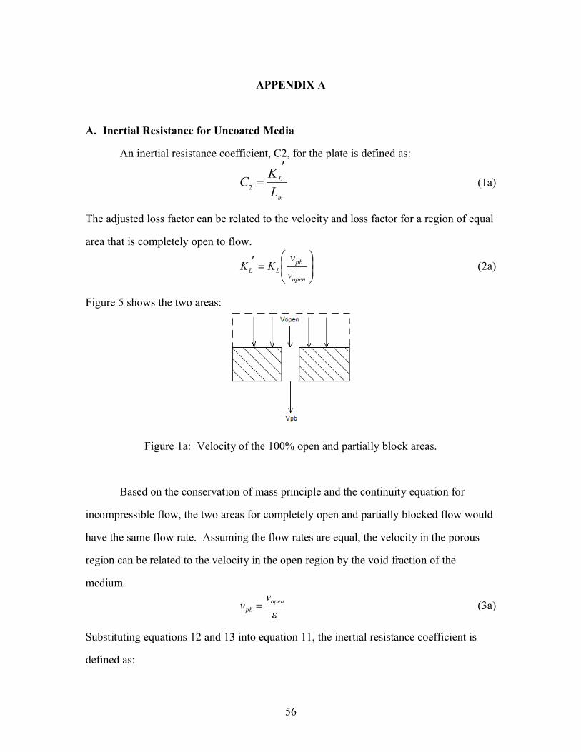
56

APPENDIX A

A. Inertial Resistance for Uncoated Media

An inertial resistance coefficient, C2, for the plate is defined as:

m

L

LKC

′=2 (1a)

The adjusted loss factor can be related to the velocity and loss factor for a region of equal

area that is completely open to flow.

=′

open

pbLL v

vKK (2a)

Figure 5 shows the two areas:

Figure 1a: Velocity of the 100% open and partially block areas.

Based on the conservation of mass principle and the continuity equation for

incompressible flow, the two areas for completely open and partially blocked flow would

have the same flow rate. Assuming the flow rates are equal, the velocity in the porous

region can be related to the velocity in the open region by the void fraction of the

medium.

εopen

pb

vv = (3a)

Substituting equations 12 and 13 into equation 11, the inertial resistance coefficient is

defined as:

57

2

2

1

=

εm

L

LKC (4a)`

58

APPENDIX B

B. Surface Tension at Substrate/Air Interface

In order to estimate the surface tension at the substrate/air interface, we can look at the

case of two semi-infinite substrates in contact with each other. The surface energy of the

two substrates when not in contact with each other, but in contact with the air between

the substrates, is equal to 2σSA. When in contact with each other, the surface energy is

equal to the van der Waals energy between the two substrates.

02 =− SSSA Vσ (1b)

2SS

SA

V=σ (2b)

The van der Waal energy is defined as:2

SSS akV ∗= (3b)

The spreading parameter, S, can be related to the van der Waals interactions through the

following relationship:

LLSL VVS −= (4b)

The spreading parameter can also be related to the contact angle, θ.

( )1cos −= θσ LAS (5b)

Substituting equation 5b into equation 4b results in the following equation:

( ) LLSLLA VV −=− )1cosθσ (6b)

For two semi-infinite identical liquids:

02 =− LLLA Vσ (7b)

LALLV σ2= (8b)

The van der Waals energy can also be defined as:2

LLL akV ∗= (9b)

Substituting equation 9b into equation 8b results in the following relationship for electric

polarisability of the liquid:

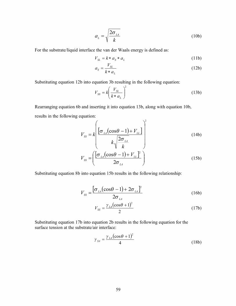
59

ka LA

L

σ2= (10b)

For the substrate/liquid interface the van der Waals energy is defined as:

LSSL aakV ∗∗= (11b)

L

SLS ak

Va∗

= (12b)

Substituting equation 12b into equation 3b resulting in the following equation:2

∗

=L

SLSS ak

VkV (13b)

Rearranging equation 6b and inserting it into equation 13b, along with equation 10b,

results in the following equation:

( )[ ]2

21cos

+−

=

kk

VkVLA

LLLASS σ

θσ(14b)

( )[ ]

+−=

LA

LLLASS

VVσ

θσ2

1cos 2

(15b)

Substituting equation 8b into equation 15b results in the following relationship:

( )[ ]LA

LALASSV

σσθσ

221cos 2+−

= (16b)

( )2

1cos 2+=

θγ LASSV (17b)

Substituting equation 17b into equation 2b results in the following equation for the surface tension at the substrate/air interface:

(18b)( )

41cos 2+

=θγ

γ LASA

60

APPENDIX C

C. Dimensional Analysis

Important Variables = f(h,d,H,D,V,ρ,μ,σ,ε,t)

Basic Units = M (mass), L (length), T (time)

Repeating Variables: D, V, μ

# Variables = 10

# Repeating Variables = 3

# Pi Terms = 10-3 = 7

cbaVhD µπ =1cb

a

LTM

TLLLTLM

= )(000

a=-1

b=0

c=0

Dh

=1π

cbaVdD µπ =2cb

a

LTM

TLLLTLM

= )(000

a=-1

b=0

c=0

61

Dd

=2π

cbaVHD µπ =3cb

a

LTM

TLLLTLM

= )(000

a=-1

b=0

c=0

DH

=3π

cbaVD µρπ =4cb

a

LTM

TLL

LMTLM

= )(3

000

a=1

b=1

c=-1

Re4 ==µ

ρπ VD

cbaVD µσπ =5cb

a

LTM

TLL

TMTLM

= )(2

000

a=0

b=-1

c=-1

62

µσπ

V=5

cbaVD µεπ =6

a=0

b=0

c=0

επ =6

cbaVtD µπ =7cb

a

LTM

TLLTTLM

= )(000

a=-1

b=1

c=0

DtV

=7π

The aspect ratio (r) is equal to π2/π1.

hd

DhDd

r ===1

2

ππ

The aspect ratio, r, will be substituted into the dimensional analysis for π2.

hdr ==2π

63

The term π4 can be divided by π5 in order to produce the Weber number.

σρ

µσµ

ρ

ππ DV

V

VD

We2

5

4 ===

The Weber number will be substituted for π5.

σρ

πDVWe

2

5 ==

The term π7 can be divided by π3 to create the following parameter, τ.

HtV

DHDtV

===3

7

ππ

τ

The parameter τ will be substituted into the analysis for π7.

HtV

== τπ 7

64

APPENDIX D

D. Aspect Ratio Correlation

Aspect Ratio Worksheet:

Knownsi fi^2 fi π1 π2 π3 π4 π5 π6 π71 0.0006 -0.02 0.50 2.50 1.75 1002.98 0.31 0.56 4.352 0.0011 -0.03 0.46 2.82 1.75 1002.98 0.31 0.56 10.863 0.0004 -0.02 0.46 2.73 1.75 1002.98 0.31 0.56 21.734 0.0015 -0.04 0.46 2.73 1.75 1002.98 0.31 0.56 43.455 0.0041 0.06 0.43 2.80 1.87 949.47 0.37 0.62 4.196 0.0000 0.00 0.43 2.90 1.87 949.47 0.37 0.62 10.487 0.0001 0.01 0.39 3.33 1.87 949.47 0.37 0.62 20.968 0.0032 0.06 0.35 3.75 1.87 949.47 0.37 0.62 41.929 0.0002 0.02 0.29 5.29 1.75 1012.76 1.11 0.79 4.3910 0.0000 0.00 0.27 5.85 1.75 1012.76 1.11 0.79 10.9711 0.0016 -0.04 0.27 6.00 1.75 1012.76 1.11 0.79 21.9412 0.0002 -0.01 0.25 6.50 1.75 1012.76 1.11 0.79 43.8813 0.0071 0.08 0.48 2.44 1.35 1055.98 0.23 0.31 4.3414 0.0007 0.03 0.48 2.52 1.35 1055.98 0.23 0.31 10.84

65

15 0.0000 0.00 0.46 2.69 1.35 1055.98 0.23 0.31 21.6816 0.0000 0.00 0.45 2.80 1.35 1055.98 0.23 0.31 43.3517 0.0047 -0.07 0.55 2.17 2.50 850.84 0.22 0.31 4.1818 0.0001 -0.01 0.50 2.27 2.50 850.84 0.22 0.31 10.4519 0.0007 -0.03 0.50 2.27 2.50 850.84 0.22 0.31 20.9020 0.0000 0.01 0.45 2.50 2.50 850.84 0.22 0.31 41.7921 0.0047 -0.07 0.53 2.22 2.88 694.07 0.16 0.31 3.6422 0.0004 0.02 0.47 2.38 2.88 694.07 0.16 0.31 9.0923 0.0000 0.00 0.47 2.38 2.88 694.07 0.16 0.31 18.1924 0.0003 -0.02 0.47 2.38 2.88 694.07 0.16 0.31 36.3825 0.0001 -0.01 0.54 2.14 1.96 862.45 0.19 0.31 3.8726 0.0006 -0.02 0.50 2.38 1.96 862.45 0.19 0.31 9.6727 0.0000 0.00 0.46 2.58 1.96 862.45 0.19 0.31 19.3328 0.0003 -0.02 0.46 2.58 1.96 862.45 0.19 0.31 38.6629 0.0001 0.01 0.62 1.50 4.92 613.43 0.20 0.31 4.3830 0.0002 -0.02 0.62 1.50 4.92 613.43 0.20 0.31 10.9531 0.0029 0.05 0.62 1.38 4.92 613.43 0.20 0.31 21.9132 0.0011 0.03 0.62 1.38 4.92 613.43 0.20 0.31 43.81

VariablesC a1 a2 a3 a4 a5 a6 a7

0.33 -1.6 -1-

0.09 0.13953 -0.1 0.03 -0.03

Constraintsa4 >/= 0a4 </= 1

Optimal Equation0.037

66

APPENDIX E

E. Visual Basic Code for Uncertainty

Sub Pi2_Uncoated_Uncertainty()Dim jRow As IntegerDim D, p, V, s, E, hd, H, u, t As VariantDim dD, Dp, dV, ds, dE, dhd, dH, du, dt As VariantDim UD, Up, UV, Us, UE, Uhd, UH, Uu, Ut As VariantDim Td, UTd, Gst, UGst, O, UO As VariantDim Wd, UWd, Lm, ULm, Ls, ULs, pf, Upf As VariantDim Pi2, Upi2 As Variant

Sheets("Uncoated_Data").Select

For jRow = 0 To 27 'Get Variables:

D = Range("I12").Offset(jRow, 0)p = Range("H5")V = Range("E12").Offset(jRow, 0)s = Range("G12").Offset(jRow, 0)E = Range("F12").Offset(jRow, 0)hd = Range("L12").Offset(jRow, 0)H = Range("J12").Offset(jRow, 0)u = Range("H6")t = Range("C12").Offset(jRow, 0)

'Find pi2 term derivatives: dD = 0.569 * ((D ^ 0.735 * p ^ 0.0889 * V ^ 0.0106 * s ^ 0.0506 * E ^ 0.0302) /

(hd ^ 1.56 * H ^ 0.0584 * u ^ 0.1395 * t ^ 0.0277))Dp = 0.029 * ((D ^ 1.735 * p ^ -0.9111 * V ^ 0.0106 * s ^ 0.0506 * E ^ 0.0302) /

(hd ^ 1.56 * H ^ 0.0584 * u ^ 0.1395 * t ^ 0.0277))dV = 0.0035 * ((D ^ 1.735 * p ^ 0.0889 * V ^ -0.9894 * s ^ 0.0506 * E ^ 0.0302) /

(hd ^ 1.56 * H ^ 0.0584 * u ^ 0.1395 * t ^ 0.0277))ds = 0.0166 * ((D ^ 1.735 * p ^ 0.0889 * V ^ 0.0106 * s ^ -0.9494 * E ^ 0.0302) /

(hd ^ 1.56 * H ^ 0.0584 * u ^ 0.1395 * t ^ 0.0277))dE = 0.0099 * ((D ^ 1.735 * p ^ 0.0889 * V ^ 0.0106 * s ^ 0.0506 * E ^ -0.9698) /

(hd ^ 1.56 * H ^ 0.0584 * u ^ 0.1395 * t ^ 0.0277))dhd = -0.512 * ((D ^ 1.735 * p ^ 0.0889 * V ^ 0.0106 * s ^ 0.0506 * E ^ 0.0302) /

(hd ^ 2.56 * H ^ 0.0584 * u ^ 0.1395 * t ^ 0.0277))dH = -0.019 * ((D ^ 1.735 * p ^ 0.0889 * V ^ 0.0106 * s ^ 0.0506 * E ^ 0.0302) /

(hd ^ 1.56 * H ^ 1.0584 * u ^ 0.1395 * t ^ 0.0277))du = -0.0458 * ((D ^ 1.735 * p ^ 0.0889 * V ^ 0.0106 * s ^ 0.0506 * E ^ 0.0302) /

(hd ^ 1.56 * H ^ 0.0584 * u ^ 1.1395 * t ^ 0.0277))

67

dt = -0.009 * ((D ^ 1.735 * p ^ 0.0889 * V ^ 0.0106 * s ^ 0.0506 * E ^ 0.0302) / (hd ^ 1.56 * H ^ 0.0584 * u ^ 0.1395 * t ^ 1.0277))

'Uncertainties:UD = 0.001 * DUp = 0.005 * pUhd = 0.001 * hdUH = 0.001 * HUu = 0.005 * uUt = 0.001 * t

'Velocity Uncertainty:Td = Range("K12").Offset(jRow, 0)UTd = 0.001 * TdUV = (1 / V) * ((UH / Td) ^ 2 + ((H * UTd) / Td ^ 2) ^ 2) ^ (1 / 2)

'Surface Tension Uncertainty:Gst = Range("H7")O = Range("M12").Offset(jRow, 0) * (3.14 / 180)UGst = 0.005 * GstUO = 0.001 * O

Us = (1 / s) * (((UO * Gst * Sin(O) * (Cos(O) - 1)) / 2) ^ 2 + UO ^ 2 * ((Cos(O) ^ 2 - 2 * Cos(O) + 1) ^ 2) / 16) ^ (1 / 2)

'Void Fraction Uncertainty:Wd = Range("H12").Offset(jRow, 0)Lm = Range("D12").Offset(jRow, 0)Ls = Range("H9")pf = Range("H8")UWd = 0.004 * WdULm = 0.001 * LmULs = 0.001 * LsUpf = 0.005 * pfUE = (1 / E) * ((UWd / (Lm * Ls ^ 2 * pf)) ^ 2 + ((ULm * Wd) / (Lm ^ 2 * Ls ^ 2

* pf)) ^ 2 + 4 * ((Wd * ULs) / (Lm * Ls ^ 3 * pf)) ^ 2 + ((Wd * Upf) / (Lm * Ls ^ 2 * pf ^ 2)) ^ 2) ^ (1 / 2)

'Pi2 Uncertainty:Pi2 = Range("N12").Offset(jRow, 0)Upi2 = (1 / Pi2) * ((dD * UD) ^ 2 + (Dp * Up) ^ 2 + (dV * UV) ^ 2 + (ds * Us) ^ 2

+ (dE * UE) ^ 2 + (dhd * Uhd) ^ 2 + (dH * UH) ^ 2 + (du * Uu) ^ 2 * (dt * Ut) ^ 2) ^ (1 / 2)

Range("O12").Offset(jRow, 0) = Upi2Range("S12").Offset(jRow, 0) = UERange("T12").Offset(jRow, 0) = UsRange("U12").Offset(jRow, 0) = UV

68

Next jRowEnd Sub

Sub Uncoated_Model_Uncertainty()Dim iRow As IntegerDim Td, UTd, G, UG, H, UH, V, UV, Vo, UVo As VariantDim a, Ua, DPerm, UDPerm, K, UK, SVoid As VariantDim KL, Lm, E, UKL, ULm, UE, C2, UC2 As Variant

'Output Void Fraction & Surface Tension Uncertainties:Pi2_Uncoated_Uncertainty

For iRow = 0 To 27 'Permeability Uncertainty:K = Range("P12").Offset(iRow, 0)SVoid = 1 - Range("F12").Offset(iRow, 0)DPerm = 1.64 * Exp(-14.421 * SVoid)UDPerm = 0.02 * DPerma = Range("R12").Offset(iRow, 0)Ua = 0.001 * aUK = (1 / K) * ((a ^ 2 * UDPerm) ^ 2 + (2 * a * DPerm * Ua) ^ 2) ^ (1 / 2)Range("V12").Offset(iRow, 0) = UK

'Inertial Resistance Uncertainty:KL = 0.5UKL = 0.005 * KLLm = Range("D12").Offset(iRow, 0)ULm = 0.001 * LmE = Range("F12").Offset(iRow, 0)UE = Range("S12").Offset(iRow, 0)C2 = Range("Q12").Offset(iRow, 0)UC2 = (1 / C2) * (((2 * KL * UE) / (Lm * E ^ 3)) ^ 2 + ((KL * ULm) / (Lm ^ 2 * E

^ 2)) ^ 2 + (UKL / (Lm * E ^ 2)) ^ 2) ^ (1 / 2)Range("W12").Offset(iRow, 0) = UC2

Next iRowEnd Sub

Sub Pi2_Coated_Uncertainty()Dim jRow As IntegerDim D, p, V, s, E, hd, H, u, t As VariantDim dD, Dp, dV, ds, dE, dhd, dH, du, dt As VariantDim UD, Up, UV, Us, UE, Uhd, UH, Uu, Ut As VariantDim Td, UTd, Gst, UGst, O, UO As Variant

69

Dim G, UG, Lm, ULm, ps, Ups As VariantDim Pi2, Upi2 As Variant

Sheets("Coated_Data").Select

For jRow = 0 To 3

'Get Variables:D = Sheets("Coated_Data").Range("I12").Offset(jRow, 0)p = Sheets("Coated_Data").Range("H5")V = Sheets("Coated_Data").Range("E12").Offset(jRow, 0)s = Sheets("Coated_Data").Range("G12").Offset(jRow, 0)E = Sheets("Coated_Data").Range("F12").Offset(jRow, 0)hd = Sheets("Coated_Data").Range("L12").Offset(jRow, 0)H = Sheets("Coated_Data").Range("J12").Offset(jRow, 0)u = Sheets("Coated_Data").Range("H6")t = Sheets("Coated_Data").Range("C12").Offset(jRow, 0)

'Find pi2 term derivatives: dD = 0.569 * ((D ^ 0.735 * p ^ 0.0889 * V ^ 0.0106 * s ^ 0.0506 * E ^ 0.0302) /

(hd ^ 1.56 * H ^ 0.0584 * u ^ 0.1395 * t ^ 0.0277))Dp = 0.029 * ((D ^ 1.735 * p ^ -0.9111 * V ^ 0.0106 * s ^ 0.0506 * E ^ 0.0302) /

(hd ^ 1.56 * H ^ 0.0584 * u ^ 0.1395 * t ^ 0.0277))dV = 0.0035 * ((D ^ 1.735 * p ^ 0.0889 * V ^ -0.9894 * s ^ 0.0506 * E ^ 0.0302) /

(hd ^ 1.56 * H ^ 0.0584 * u ^ 0.1395 * t ^ 0.0277))ds = 0.0166 * ((D ^ 1.735 * p ^ 0.0889 * V ^ 0.0106 * s ^ -0.9494 * E ^ 0.0302) /

(hd ^ 1.56 * H ^ 0.0584 * u ^ 0.1395 * t ^ 0.0277))dE = 0.0099 * ((D ^ 1.735 * p ^ 0.0889 * V ^ 0.0106 * s ^ 0.0506 * E ^ -0.9698) /

(hd ^ 1.56 * H ^ 0.0584 * u ^ 0.1395 * t ^ 0.0277))dhd = -0.512 * ((D ^ 1.735 * p ^ 0.0889 * V ^ 0.0106 * s ^ 0.0506 * E ^ 0.0302) /

(hd ^ 2.56 * H ^ 0.0584 * u ^ 0.1395 * t ^ 0.0277))dH = -0.019 * ((D ^ 1.735 * p ^ 0.0889 * V ^ 0.0106 * s ^ 0.0506 * E ^ 0.0302) /

(hd ^ 1.56 * H ^ 1.0584 * u ^ 0.1395 * t ^ 0.0277))du = -0.0458 * ((D ^ 1.735 * p ^ 0.0889 * V ^ 0.0106 * s ^ 0.0506 * E ^ 0.0302) /

(hd ^ 1.56 * H ^ 0.0584 * u ^ 1.1395 * t ^ 0.0277))dt = -0.009 * ((D ^ 1.735 * p ^ 0.0889 * V ^ 0.0106 * s ^ 0.0506 * E ^ 0.0302) /

(hd ^ 1.56 * H ^ 0.0584 * u ^ 0.1395 * t ^ 1.0277)) 'Uncertainties:UD = 0.001 * DUp = 0.005 * pUhd = 0.001 * hdUH = 0.001 * HUu = 0.005 * u

Ut = 0.001 * t

70

'Velocity Uncertainty:Td = Sheets("Coated_Data").Range("K12").Offset(jRow, 0)UTd = 0.001 * TdUV = (1 / V) * ((UH / Td) ^ 2 + ((H * UTd) / Td ^ 2) ^ 2) ^ (1 / 2)

'Surface Tension Uncertainty:Gst = Sheets("Coated_Data").Range("H7")O = Sheets("Coated_Data").Range("M12").Offset(jRow, 0) * (3.14 / 180)UGst = 0.005 * GstUO = 0.001 * O

Us = (1 / s) * (((UO * Gst * Sin(O) * (Cos(O) - 1)) / 2) ^ 2 + UO ^ 2 * ((Cos(O) ^ 2 - 2 * Cos(O) + 1) ^ 2) / 16) ^ (1 / 2)

'Void Fraction Uncertainty:G = Sheets("Coated_Data").Range("H12").Offset(jRow, 0)Lm = Sheets("Coated_Data").Range("D12").Offset(jRow, 0)ps = Sheets("Coated_Data").Range("H8")UG = 0.0025 * GULm = 0.001 * LmUps = 0.005 * psUE = (1 / E) * ((UG / (Lm * ps)) ^ 2 + ((G * ULm) / (ps * Lm ^ 2)) ^ 2 + ((Ups *

G) / (ps ^ 2 * Lm)) ^ 2) ^ (1 / 2) Pi2 = Sheets("Coated_Data").Range("N12").Offset(jRow, 0)Upi2 = (1 / Pi2) * ((dD * UD) ^ 2 + (Dp * Up) ^ 2 + (dV * UV) ^ 2 + (ds * Us) ^ 2

+ (dE * UE) ^ 2 + (dhd * Uhd) ^ 2 + (dH * UH) ^ 2 + (du * Uu) ^ 2 * (dt * Ut) ^ 2) ^ (1 / 2)

Sheets("Coated_Data").Range("O12").Offset(jRow, 0) = Upi2Sheets("Coated_Data").Range("S12").Offset(jRow, 0) = UESheets("Coated_Data").Range("T12").Offset(jRow, 0) = UsSheets("Coated_Data").Range("U12").Offset(jRow, 0) = UV

Next jRowEnd Sub

Sub Coated_Model_Uncertainty()Dim iRow As IntegerDim Td, UTd, G, UG, H, UH, V, UV, Vo, UVo As VariantDim Dp, UDp, E, UE, K, UK As VariantDim C2, UC2 As Variant

'Output Void Fraction & Surface Tension Uncertainties:Pi2_Coated_Uncertainty

For iRow = 0 To 3

71

'Permeability & Inertial Resistance Uncertainty:K = Sheets("Coated_Data").Range("P12").Offset(iRow, 0)C2 = Sheets("Coated_Data").Range("Q12").Offset(iRow, 0)Dp = Sheets("Coated_Data").Range("R12").Offset(iRow, 0)E = Sheets("Coated_Data").Range("F12").Offset(iRow, 0)UDp = 0.01 * DpUE = Sheets("Coated_Data").Range("S12").Offset(iRow, 0)UK = (1 / K) * (((UDp * Dp * E ^ 3) / (75 * (1 - E) ^ 2)) ^ 2 + ((UE * Dp ^ 2 * E ^

2 * (E - 3)) / (150 * (E - 1) ^ 3)) ^ 2) ^ (1 / 2)UC2 = (1 / C2) * (((3.5 * UDp * (E - 1)) / (Dp ^ 2 * E ^ 3)) ^ 2 + ((7 * UE * (E -

1.5)) / (Dp * E ^ 4)) ^ 2) ^ (1 / 2)Sheets("Coated_Data").Range("V12").Offset(iRow, 0) = UKSheets("Coated_Data").Range("W12").Offset(iRow, 0) = UC2

Next iRowEnd Sub