modeling solar cosmic ray transport within the ecliptic …nbn:de:gbv:... · department of physics...
TRANSCRIPT

Department of Physics
Modeling Solar Cosmic Ray Transport within theEcliptic Plane
A PhD Thesis submitted for the
degree of Doctor of Science (Dr. rer. nat.)
by Dipl. Systemwiss. Florian Lampa
Osnabruck, February 23, 2011


Supervisor, First reviewer:
Prof. Dr. May-Britt KallenrodeUniversitat OsnabruckFachbereich PhysikBarbarastraße 749069 Osnabruck
Second reviewer:
Prof. Dr. Philipp MaaßUniversitat OsnabruckFachbereich PhysikBarbarastraße 749069 Osnabruck


Abstract
Since six decades the understanding of interplanetary propagation of solar flare acceler-ated, energetic charged particles in the inner heliosphere has not yet achieved sufficientclosure. The essential mechanisms acting on these charged particles, which performhelical orbits along the large-scale magnetic field lines as probes, have already beenidentified. However, in particular the impact of the three-dimensional, small-scale mag-netic fluctuations on the particles’ trajectories has not yet been fully understood. Thesesuperimposed disturbances are expected to interact with the charges via resonance prin-ciple – leading to both field-aligned scattering and diffusive cross-field displacements ofthe particles’ guiding center.Since numerical solutions and known theoretical formulations have failed to verify themeasurements so far, Ruffolo’s equation – which is a special formulation of the Fokker-Planck equation – is applied to take account of the current knowledge about field-paralleltransport; The partial differential equation is extended to a two-dimensional model withinthe ecliptic plane by a spatial diffusion term perpendicular to the field. We assume anidealized Archimedean field neither with polarity changes nor large-scale disturbancessuch as traveling magneto-hydrodynamic shock waves or magnetic clouds.The transport equation is solved numerically by finite differences. For typical ratios of per-pendicular to parallel diffusion coefficient as deduced from theory, various fits have beenfound in good agreement with multi-spacecraft measurements. Some events and theoccurrence of observed sudden flux drop-outs suggest that scattering on magnetic fieldirregularities significantly varies from one flux tube to another. In addition to the alreadyexisting, but sparse set of particle observations at different positions, once the currentsolar minimum has passed by, a new set will be available from the recently launchedSTEREO satellites.

Zusammenfassung
Die interplanetare Ausbreitung von hochenergetischen, geladenen Teilchen, die inner-halb der inneren Heliosphare durch solare Flares freigesetzt werden, ist auch nach 6Jahrzehnten astrophysikalischer Forschung nicht ausreichend verstanden. Die wichtig-sten, auf diese geladenen Partikel wirkenden Mechanismen wurden bereits erfasst: So-lare energiereiche Teilchen breiten sich wie Testteilchen spiralformig entlang der großskali-gen Magnetfeldlinien aus. Dennoch ist insbesondere der Einfluss der drei-dimensionalen,kleinskaligen Magnetfeld-Fluktuationen auf die Teilchenpfade noch nicht vollstandig ver-standen. Man vermutet, dass diese uberlagerten Storungen via Resonanzprinzip mitden Ladungen wechselwirken, was sowohl zu feldparalleler Streuung als auch diffusiven,senkrechten Verschiebungen der Trajektorien fuhren kann.Da bisherige theoretische Betrachtungen die Beobachtungen nicht im ausreichendenMaß verifizieren konnten, wird die Ruffolo-Gleichung verwendet – eine spezielle For-mulierung der Fokker-Planck Gleichung – um das aktuelle Wissen um feld-parallelenTransport zu berucksichtigen; die partielle Differentialgleichung ist mittels eines additivenraumlichen Diffusionskoeffizienten in feldsenkrechter Richtung zu einem zwei-dimensio-nalen Model ausgebaut worden (die Ekliptikalebene reprasentierend). Es wird ein ide-alisiertes, archimedisches Spiralfeld angenommen, in dem es weder Polaritatswechselnoch Storungen wie z.B. laufende magneto-hydrodynamische Shockwellen oder mag-netische Wolken gibt.Die Transport-Gleichung wird mittels Finiter Differenzen numerisch gelost. Mittels typis-cher, aus der Theorie stammender Verhaltnisse zwischen senkrechtem und parallelemDiffusionskoeffizienten sind als Ergebnis eine Vielzahl von Fits ermittelt worden, die inguter Ubereinstimmung mit dem simultanen Messungen zweier Raumfahrzeuge sind.Einige Teilchen-Ereignisse und das Auftreten abrupter Einbruche in den Flussen niederen-ergetischer Protonen lassen vermuten, dass sich die Streueigenschaften des interpla-netaren Mediums deutlich von einer Flußrohre zur nachsten andern konnen. Nebender bereits vorhandenen, aber nicht sehr umfangreichen Datensammlung von Teilchen-beoachtungen an verschiedenen Positionen wird es demnachst zusatzliches Datenma-terial von den STEREO-Satelliten geben, zumal das aktuelle solare Minimum in Kurzedurchlaufen sein wird.

Contents
1. Introduction 9
2. Energetic Particles in the Inner Heliosphere 112.1. Charged particles in electromagnetic fields . . . . . . . . . . . . . . . . . . 11
2.1.1. Single particle motions . . . . . . . . . . . . . . . . . . . . . . . . . . 112.1.2. Magnetohydrodynamics (MHD) . . . . . . . . . . . . . . . . . . . . 15
2.2. Solar structure and its magnetic field . . . . . . . . . . . . . . . . . . . . . 192.3. Sources of solar energetic particles . . . . . . . . . . . . . . . . . . . . . . 222.4. Interplanetary propagation of SEPs . . . . . . . . . . . . . . . . . . . . . . 24
2.4.1. SEP motion along the average interplanetary magnetic field . . . . 242.4.2. Resonance scattering . . . . . . . . . . . . . . . . . . . . . . . . . . 272.4.3. Changes to momentum . . . . . . . . . . . . . . . . . . . . . . . . . 312.4.4. Measurands . . . . . . . . . . . . . . . . . . . . . . . . . . . . . . . 32
3. Modeling in 2-D 353.1. Conventional modeling of solar energetic particle transport . . . . . . . . . 353.2. An extended and modified model version . . . . . . . . . . . . . . . . . . . 37
3.2.1. Model equation . . . . . . . . . . . . . . . . . . . . . . . . . . . . . 393.2.2. Choice of the grid . . . . . . . . . . . . . . . . . . . . . . . . . . . . 43
4. Numerics in Non-equidistant Grids 514.1. Basics of the Finite-Difference Method . . . . . . . . . . . . . . . . . . . . . 51
4.1.1. Consistency of finite differences . . . . . . . . . . . . . . . . . . . . 514.1.2. Stability . . . . . . . . . . . . . . . . . . . . . . . . . . . . . . . . . . 524.1.3. Summarized approximation method . . . . . . . . . . . . . . . . . . 53
4.2. Transport along an IMF line (s-transport) . . . . . . . . . . . . . . . . . . . 554.3. Transport in pitch-cosine . . . . . . . . . . . . . . . . . . . . . . . . . . . . 604.4. Adiabatic deceleration (momentum-transport) . . . . . . . . . . . . . . . . . 614.5. Transport perpendicular to the IMF . . . . . . . . . . . . . . . . . . . . . . . 63
4.5.1. Consistency . . . . . . . . . . . . . . . . . . . . . . . . . . . . . . . . 644.5.2. Stability . . . . . . . . . . . . . . . . . . . . . . . . . . . . . . . . . . 67
4.6. Initial and boundary conditions . . . . . . . . . . . . . . . . . . . . . . . . . 69
5. Simulation Assumptions 735.1. SEP injections and boundary conditions . . . . . . . . . . . . . . . . . . . . 735.2. Assumptions regarding field-parallel transport . . . . . . . . . . . . . . . . 745.3. Strength and variability of the perpendicular diffusion coefficient κ⊥ . . . . 75
5.3.1. Does cross-field transport depend on rigidity? . . . . . . . . . . . . 775.4. The standard scenario . . . . . . . . . . . . . . . . . . . . . . . . . . . . . 79
6. Validation and Tests 816.1. Field-parallel Transport . . . . . . . . . . . . . . . . . . . . . . . . . . . . . 81
7

6.2. Field perpendicular transport . . . . . . . . . . . . . . . . . . . . . . . . . . 836.3. Azimuthal vs. perpendicular cross-field transport . . . . . . . . . . . . . . . 876.4. Introduction of solar wind effects . . . . . . . . . . . . . . . . . . . . . . . . 886.5. Spatial resolution . . . . . . . . . . . . . . . . . . . . . . . . . . . . . . . . . 90
7. Model Results 957.1. A parameter study . . . . . . . . . . . . . . . . . . . . . . . . . . . . . . . . 95
7.1.1. Plots in the ecliptic plane . . . . . . . . . . . . . . . . . . . . . . . . 957.1.2. Cross-field profiles . . . . . . . . . . . . . . . . . . . . . . . . . . . . 987.1.3. Intensity-time and anisotropy-time profiles . . . . . . . . . . . . . . 100
7.2. Observations . . . . . . . . . . . . . . . . . . . . . . . . . . . . . . . . . . . 1067.2.1. Intensities varying with connection to the flare site . . . . . . . . . . 1067.2.2. Fitting both intensity- and anisotropy profiles . . . . . . . . . . . . . 1107.2.3. Diffusion as the big leveler vs. sudden flux dropouts . . . . . . . . . 121
8. Conclusions and Outlook 125
A. Appendix 127A.1. Physical quantities and acronyms . . . . . . . . . . . . . . . . . . . . . . . 127A.2. Program details . . . . . . . . . . . . . . . . . . . . . . . . . . . . . . . . . . 128
A.2.1. Structure . . . . . . . . . . . . . . . . . . . . . . . . . . . . . . . . . 128A.2.2. Installation . . . . . . . . . . . . . . . . . . . . . . . . . . . . . . . . 131A.2.3. Parallelization . . . . . . . . . . . . . . . . . . . . . . . . . . . . . . 133
A.3. User interfaces . . . . . . . . . . . . . . . . . . . . . . . . . . . . . . . . . . 135A.4. Numerically solved flux tubes . . . . . . . . . . . . . . . . . . . . . . . . . . 138A.5. Various intensity-time profiles for ∼0.5 MeV electrons . . . . . . . . . . . . 140

1. Introduction
The main issue of this PhD thesis will be to investigate the propagation of solar ener-getic particles (SEPs) in the inner heliosphere - an area covering about three astronom-ical units (AU) around the Sun. SEPs mainly consist of charged particles as electrons,protons and α-particles – their energies range in the MeV domain. Neutral atoms andmolecules are not present since the hard electromagnetic radiation (e.g. X-rays) ionizesall matter. Moreover, ionization occurs by heating to such high temperatures that therandom kinetic energy of the molecules exceeds the ionization energy.First indirect evidences of charged particles were found in 1911-12 by balloon flights in theEarth’s atmosphere (Gockel, 1911; Hess, 1912). But the particles causing these chargeshave their origin beyond the heliosphere (galactic cosmic rays, GCRs). Three decadeslater, the SEPs (also called “solar cosmic rays”) could be detected indirectly by ground-based neutron monitors (Forbush, 1946): Very high-energetic particles, sometimes emit-ted during solar events, interact with atmospheric molecules/ atoms, which themselvesare split into smaller pieces. Each of them still has sufficient energy to interact with othercomponents. The process continues and is termed an “atmospheric cascade”. If theprimary cosmic ray that started the cascade has an energy above 500 MeV, some ofits secondary byproducts (including neutrons) will reach ground level where they can bedetected by neutron monitors. Correlations of the neutron counting rates to the largestsolar outbursts (ground level events, GLEs) showed, that these charged particles hittingthe upper atmosphere originate from the Sun. Solar energetic particles form the solarcomponent of cosmic rays. They are accelerated in the upper solar corona as well as ininterplanetary space. SEPs are not allowed to be confused with the continuously outwardstreaming solar wind plasma. This plasma is less energetic. As part of the solar corona(the Sun’s atmosphere), it is accelerated (heated up) and, as a consequence, a hydro-dynamic expansion (Parker, 1958) into space occurs. Solar wind speeds vary between300 km s−1 and 800 km s−1. Near the heliomagnetic equator, the solar wind propagatesmore slowly than in polar regions and is directed radially outward. On its way out, the so-lar wind shapes the local magnetic field structure of the Sun because the plasma energydensity is higher than the field’s energy density (frozen-in magnetic fields, Alfven, 1976,and references therein). Since the Sun rotates with a sidereal period of about 27 days,the base of each field line frozen into the solar wind plasma is carried westward - formingan Archimedean spiral.The interplanetary magnetic field (IMF) is one of the essential parts to describe the prop-agation of SEPs: Once they have been accelerated, the charged particles mainly prop-agate along the magnetic field lines – guided by the Lorenz force, which keeps them onhelical orbits. The particle’s velocity components are mainly field-parallel aligned as seenin the anisotropies (Fisk and Axford, 1969; Jokipii, 1966). Other transport mechanismsas well as small-scale disturbances in the IMF have already been identified, too. Besidesconvection along the IMF lines, there are scattering on magnetic irregularities, focusing inthe diverging IMF as well as adiabatic deceleration (cooling) of the expanding particles,and convection due to the solar wind.
9

10 CHAPTER 1. INTRODUCTION
Interplanetary transport of SEPs has been regarded essentially as spatially one-dimen-sional: particles gyrate around the interplanetary magnetic field and are scattered backand forth along it at magnetic field inhomogeneities. But some observations in the earlypast, that also looked beyond the field lines particles have been injected on, have sug-gested that solar cosmic rays were transported oblique to the field. An estimate about theefficiency of cross-field transport is not as easy as it seems: Energetic particles do notform a homogeneous bulk but are manifold and temporally variable in many ways. Thus,energetic particles in interplanetary space must have their origin in different sources. Butthese sources of acceleration do not necessarily take place in the upper corona – more-over they are not expected to be implicitly located at confined, point-like areas either.An observer remote from the source will detect particles, which represents a mixture ofboth interplanetary transport- and acceleration processes such as traveling interplane-tary shock waves. This makes the interpretation of the satellite data difficult.
It will be the purpose of this work to adopt the knowledge about interplanetary trans-port and to incorporate it into a two-dimensional model of solar particle transport in theecliptic plane. The model will be extended by momentum transport, so that accelerationprocesses such as traveling shocks can be introduced.As an introduction into space and plasma physics, Chapter 2 will provide the basic re-quirements about plasmas in interplanetary space to understand the following modelingapproaches. Chapter 3 start with the illustration of former modeling approaches. TheRuffolo’s equation is extended by additional terms within the modeled ecliptic plane. Theresulting partial differential equation (PDE) is subsequently solved numerically by a FiniteDifference scheme (see Chapter 4). Chapter 5 presents the modeling assumptions con-cerning in particular the mean free paths and the ratio of perpendicular to parallel diffu-sion. Without any physical context, Chapter 6 is dedicated to the validation the numericalcode and to the comparison of it’s output with the outputs of the preceding numericalmodel. Parameter studies are used in the first part of Chapter 7 to check the plausibil-ity of different propagation scenarios as well as the interpretation of field fluctuations asdescribed by a pitch-angle diffusion coefficient. Finally, solutions have been fitted to theobserved intensity- and anisotropy-time-profiles to obtain the scattering conditions (meanfree paths or diffusion coefficients) in interplanetary space (see Chapter 7). Conclusionsand possible new arising questions about interplanetary propagation of SEPs will illumi-nated in Section 8. The appendix A collects various numerical model details, includingthe user interfaces and the applied method of parallelization.

2. Energetic Particles in the InnerHeliosphere
With increasing distance from the Earth, the neutral components of matter, known inaggregate states “solid”, “liquid” and “gaseous” become rare, whereas the ionized matterdominates. Space is therefore dominated by plasmas, the fourth state of matter.But the variety of different plasma constituents seems to pose a big challenge in de-scribing their propagation in interplanetary space. In situ observations of the solar windshowed that the interplanetary medium was rather turbulent and permeated by sizablefluctuations of the plasma flow and density and of the magnetic field. The fluctuationsoccur on all observed spatial and temporal scales. The charged particles are introducedinto a preexisting field, which exert a force on them. The force will be different for elec-trons and protons, so currents will develop. The currents will modify the magnetic field.Thus, finding a solution to the resulting transport equations is somewhat complicated.This chapter will be addressed to this issue, which can be solved to both dense plasmas,such as the solar wind, and to solar energetic particles (SEPs), respectively.
2.1. Charged particles in electromagnetic fields
Compared to matter on Earth, densities of plasmas and solar energetic particles in theheliosphere are very low. Particles are not expected to interact with each other - neitherby direct collisions nor by Coulomb forces (an exception from this, of course, is the denseinterior of the Sun and its largest planets).
2.1.1. Single particle motions
Under these almost vacuum conditions, external electromagnetic fields can not inducefields into these conglomerate of charged particles. The permeability µ and the permit-tivity ε are both equal one: the medium can be neither magnetized nor polarized.Positive and negative charges are nearly equal, at least in larger scales of the Debeye-length (see Section 2.1.2).SEPs are much more energetic than the solar wind particles, but their energy density ismuch too low to modify the fields through which they pass. This makes them to idealprobes for studying the interplanetary magnetic field B.The amount of SEPs is highly variable from event to event – ranging from “not distinguish-able” from background plasma up to intensity increases by a few orders of magnitude.Every solar energetic particle, charged by q, will be affected by the Lorentz force:
FL = q · v ×B ≡ mdv
dt. (2.1)
It acts perpendicular to the field as well as perpendicular to the particles’s speed v. Thus,there is no energy gain within the magnetic field. In a presence of a static, homogeneousmagnetic field, charges perform a uniform circular orbit within a plane perpendicular to
11

12 CHAPTER 2. ENERGETIC PARTICLES IN THE INNER HELIOSPHERE
Figure 2.1.: The motion of a charged particle in a static magnetic field (Gurnett and Bhat-tacharjee, 2005, p. 25).
B (gyration), while they move constantly forward along the field. The resulting trajectorydescribes a helix around the field line (Figure 2.1). The direction of motion dependson the particle’s charge: Positively charged particles rotate in the left-hand sense withrespect to the magnetic field. The radius of the particle orbit, the Larmor radius rL, canbe obtained from either solving the partial differential equation (2.1) directly or from theperpendicular component of the Lorentz force, which is equivalent to the centrifugal force.Thus, (2.1) can be written:
mv2⊥rL
= |q|v⊥B .
The radius is given by:
rL =mv⊥|q|B . (2.2)
It is identical to the cyclotron radius ρc, as mentioned in the Figure 2.1. Since v⊥ isconstant, the Larmor radius is also constant. Because of ω = v
rL, the cyclotron frequency
of this harmonic oscillator is
ω =|q|Bm
. (2.3)
The instantaneous center of the rotation is called the guiding center, which moves withconstant velocity along the field for a static uniform field. The concept of guiding centerswill also useful for describing motion in non-uniform fields (Section 2.4).
Pitch angle
The pitch-angle α denotes the inclination of the particles trajectory with respect to themagnetic field; it is given by the ratio between the velocity components perpendicularand parallel to B:
tan(α) =v⊥v||
. (2.4)
It’s projection into the field direction is
µ = cos(α) , (2.5)
which is the so-called “pitch-cosine”. This quantity plays an important role in describinga single charged particle in interplanetary space. Under some constraints, the particle’s

2.1. CHARGED PARTICLES IN ELECTROMAGNETIC FIELDS 13
motion can be split up into field-parallel motion of the gyro-center and the gyro–motion.The pitch-cosine represents the projection factor of the particle’s position vector and ve-locity onto the gyro-center’s field line (see Section 2.4.1 for more details). Moreover, theµ notation has been found reasonable in terms of a theoretical formulation of diffusiveprocesses (see Section 2.4.2).
Magnetic rigidity
Magnetic rigidity P [V] describes the resistance of a charged particle to change its direc-tion in a magnetic field:
P =p⊥q. (2.6)
p⊥ is the momentum component perpendicular to B and, again, q denotes the particle’scharge. Combined with (2.2), the Larmor radius is directly related to the magnetic rigidityby rL = P/B: Particles of identical rigidity always propagate along identical orbits as longas the magnetic field configuration is static or is changing slowly (adiabatically) comparedto the particle’s motion. The direction of motion is determined by the charge sign. The-oretical studies about solar cosmic ray propagation (Hasselmann and Wibberenz, 1970,and references therein) predict, that SEPs of different rigidities are differently affected bymagnetic field fluctuations – leading to different mean free paths. Observations on theother hand, suggest λ to be independent of rigidity (Kallenrode, 1993b). Thus, this issueis still unsolved.
Magnetic moment
A charged particle moving in a circular orbit with radius rL and gyration time Tc gives riseto a ring current I = q/Tc = qωc/(2π). In analogy to electric currents within conductorloops, an angular momentum develops – trying to align the encircled conductor loop layerperpendicular to the magnetic field.The magnetic moment is defined by:
M = IAn , in [Am2] . (2.7)
The normal vector n of the area A is directed opposite to the external field. The scalarform of the magnetic momentum is given by:
M =|q|ωc2π· πr2
L =mv2⊥
2B=Wkin,⊥B
, (2.8)
using the definition of the Larmor radius (2.2) and the cyclotron frequency (2.3).The angular momentum
L = mrL × v⊥ = mrLv⊥eL (2.9)
is connected to the magnetic moment via
M =mv2⊥
2B
(2.3)=
v2⊥|q|2ω
(2.9)=|q|L
2. (2.10)
The vectorial description yields:
M =qL
2=
1
2qrL × v⊥ = −Wkin,⊥
B
B2(2.11)

14 CHAPTER 2. ENERGETIC PARTICLES IN THE INNER HELIOSPHERE
Indeed, M is always anti-parallel to B. Moreover, with no electric fields at present, it isalso a conservation quantity – like the kinetic energy – as long as B is kept constant or isjust changing slowly compared to the gyro-motion (adiabatic invariants, see next Section2.1.1 and also 2.4.1).
Adiabatic Invariants
In a nearly periodic system with slowly varying parameters – such as the external mag-netic fields – the action integral
J =
∮pdq (2.12)
is an adiabatic invariant (Goldstein, 1959). p and q denote the generalized momentumsand coordinates, respectively. This constant of motion provide a powerful tool to describemotions of charged particles in weakly and slowly varying fields. For gyro-motion, threetypes can be identified (see also e.g. Northrop, 1963):First, the field changes only slowly during one gyration. The corresponding action integralin polar coordinates is:
J = 2πmωcr2L . (2.13)
Except for some multiplicative constants, it is the same as the constancy of the magneticmoment: J = 4πmM/|q|.The second invariant says that the field only varies weakly on a scale comparable with thedistance traveled along the field by the particles. The action integral for parallel motioncan be written:
J = m
∮v‖ds , (2.14)
where the integration is along the magnetic field between two points of vanishing v‖. Theparallel velocity in (2.14) can be determined from the energy conservation equation
Ekin = Ekin,‖ + Ekin,⊥ =1
2mv2‖ +
1
2mv2⊥ ⇔MBm =
1
2mv2‖ +MB , (2.15)
so that
J =√
2Mm
∫ b
a
√Bm −B(s)ds . (2.16)
Since M is a constant according to the first invariant, the second adiabatic invariant isequivalent to requiring that the integral∫ b
a
√Bm −B(s)ds (2.17)
has to be a constant, where a and b are two points of vanishing v‖. We will address someapplications in inhomogeneous magnetic fields in Section 2.4.The third invariant (flux invariant), states that magnetic flux enclosed by the drift orbit isconstant. To proof the result, we only consider orbits near the axis of symmetry. Ac-cording to Faraday’s law, a temporally changing magnetic field produces an azimuthal,non-conservative electric field:∫
CEdl = −
∫S
∂B
∂tdt . (2.18)

2.1. CHARGED PARTICLES IN ELECTROMAGNETIC FIELDS 15
The integral is evaluated along the drift contour C. In axial symmetry and in a weaklyvarying radial magnetic field near the axis, the integrals can be evaluated and show that
2πRE = −dBdt
(πR2)
or
E = −R2
dB
dt.
The azimuthal electric field produces a radial (E×B)-drift, given by
vE =E
B= − R
2B
dB
B.
Since vE = dR/dt it follows that
2dR
R= −dB
B.
Direct integration of the above equation shows that the magnetic flux inside the drift orbitis constant:
ΦB = πR2B .
In an adiabatically varying magnetic, axially symmetric field, the particle always stays onthe surface of the drift orbit. This area is called a flux tube. Magnetic flux through thesurface of a flux tube remains constant, independent of the surface’s position. Frozen-inmagnetic fields (Section 2.1.2) can be explained by this.The partial differential equation (2.1) would reveal a theoretical model to describe particletransport in the interplanetary magnetic field (IMF), if it is combined with solar wind ef-fects, namely the convection with the solar and adiabatic deceleration (cooling) in the ex-panding solar wind (see Section 2.4). But note that the definitions, as mentioned above,were made in homogeneous and slowly varying fields under very idealized conditions.They are found adequate to describe particle propagation, but these approaches arecomplicated by the nature of the field: the nominal Archimedean spiral field is disturbedby fluctuations (waves and turbulence), the passage of transient disturbances such asmagnetic clouds and interplanetary coronal mass ejections (CMEs) and, at least beyond1 AU, corotating interaction regions. Besides these features, one has take into accountthe different acceleration mechanisms, which might vary in time and space as well (Sec-tion 2.3).
2.1.2. Magnetohydrodynamics (MHD)
The preceding section began with the discussion of individual particle motions, but plasmain general consists of a collection of particles. The macroscopic properties of a large num-ber of particles, such as density, temperature and pressure, can be described in termsof averages over small spatial volumes. The size of these regions and the time scalesof interest have to be chosen properly in order to have statistically relevant values. Theyhave to be larger than the microscopic particle motions: For example, the spatial scalesof interest have to be large with respect to the gyro-radius (2.2) and Debeye length λD.Within a gas containing both ions and electrons, λD describes the distance from an iso-lated, charged particle, where its electrostatic potential does not significantly influences

16 CHAPTER 2. ENERGETIC PARTICLES IN THE INNER HELIOSPHERE
its surroundings anymore (note that λD depends on density). Time scales of interest arelong compared with the times of single particles, e.g. the periods of the cyclotron motionT = 2π/ω (2.3) and the inverse plasma frequency. The average properties are governedby the basic conservation laws for mass, momentum, and energy in a fluid. The influenceof electric and magnetic fields as well as currents will be added – forming the equationsof magnetohydrodynamics (MHD).
Phase-space density
To carry out a statistical description of plasma, describing the properties of the plasmaand its motion (kinetic theory ), it is convenient to introduce a six-dimensional space,called the phase space. It consist of three position coordinates x, y and z, and thevelocity coordinates vx, vy and vz. The average number density of particles in a smallvolume element of phase space is called phase space density or distribution function:
dN = f(r,v, t)d3r d3v d3r = dxdydz d3v = dvxdvydvz. (2.19)
The average value of any dynamical quantity (bulk velocity, number density, pressuree.g.) can be computed by taking the integral over the distribution function.
Kinetic equations
The evolution of distribution function (2.19) in phase space is described by a differentialequation, called the Boltzmann equation. It’s derivation requires that forces F on chargedparticles are the same for all particles in a given phase space volume element. Theseexternal, long-range forces originate from collective effects of a large number of particles.According to the Newton’s law on a single particle (fixed values for v and r) it followsthat each particle has its own, unique trajectory in phase space. The trajectories do notintersect, thus all of the particles within the volume element dr3dv3 at time t are mappedinto the corresponding volume element dr′3dv′3 at time t′ = t + ∆t. The number ofparticles in the “new” volume element yields
f(v +F
m∆t, r + v∆t, t+ ∆t)dr′3dv′3 .
Small-range interactions are neglected, thus particles are not expected to change velocitywithin the time interval ∆t. Consequently, the particle number in the volume elementdr3dv3 has been completely shifted to the new volume element by changing its positionto r′ = r+v∆t and by being exposed to the external force(s) v′ = v+ F
m∆t. The differenceof particle numbers between the volume elements in primes and without primes is zero:[
f(v +F
m∆t, r + v∆t, t+ ∆t)− f(v, r, t)
]= 0 . (2.20)
Dividing (2.20) by ∆t and forming ∆t→ 0, we get the total differential of f :
∂f
∂t+ v
∂f
∂r+
F
m
∂f
∂v= 0 , (2.21)
which is the Boltzmann equation describing the evolution of the distribution function inphase space (incompressible fluid according to Liouville’s theorem). In interplanetaryspace plasmas, the external forces are described by the Lorentz force. Inserting into

2.1. CHARGED PARTICLES IN ELECTROMAGNETIC FIELDS 17
the Boltzmann equation gives rise to the Vlasov equation (Vlasov, 1938). By introducingcollisions, particles might be lost or added during time interval ∆t. As a consequence, acollision term (∂f/∂t)c is added to the right hand site of (2.21).Short-range interactions between particles (e.g. collisions) give rise to the Fokker-Planckequation. Trajectories of individual particles in phase space can not be predicted, al-though their initial positions are known. The collisions under consideration are expectedto lead to only a small change in the particle’s state. Thus, there is no direct mechanicalanalogy to Brownian motion, where particles even reverse the direction of motion afterbeing hit once by another particle.Formally, the stochastic process of collisions can be described by averaging over suffi-cient number of particles (cf. Subsection 2.1.2). Then, collective behavior can be deter-mined: The probability function Ψ(v,∆v) is defined as the probability that a particle ofvelocity v after many collisions in time interval ∆t has changed to v + ∆v:
f(r,v, t) =
∫f(r,v −∆v, t−∆t)Ψ(v −∆v,∆v)d(∆v) . (2.22)
Small angular changes are considered only, thus |∆v| << |v|. Consequently, we areallowed to expand the product f ·Ψ to second order by Taylor:
f(r,v, t) =
∫ [f(r,v, t−∆t)Ψ(v,∆v)−∆v · ∂(fΨ)
∂v
]d(∆v) (2.23)
+
∫ [∆v∆v
2 ∂2(fΨ)
∂v∂v
]d(∆v) .
Since, by definition, the probability function can be normalized by∫Ψd(∆v) = 1 ,
(2.23) simplifies to:
f(r,v, t) = f(r,v, t−∆t)− ∂(f〈∆v〉)∂v
+1
2
∂
∂v∂v (f〈∆v∆v〉) . (2.24)
The averages of ∆v and ∆v∆v over all possible changes d(∆v) are given by
〈∆v〉 =
∫Ψ∆vd(∆v) and 〈∆v∆v〉 =
∫Ψ∆v∆vd(∆v) . (2.25)
The difference of the distribution function at times t+ ∆t and t(∂f
∂t
)coll
=f(r,v, t)− f(r,v, t−∆t)
∆t(2.26)
is equivalent to the collision term, as it has been introduced in (2.21). According to (2.24)this is equivalent to:(
∂f
∂t
)coll
∆t = − ∂
∂v· (f〈∆v〉) +
1
2
∂2
∂v∂v (f〈∆v∆v〉) . (2.27)
The collision term can also formally be described by a diffusion tensor/ coefficient D:(∂f
∂t
)coll
∆t = −∇v · (D · ∇v · f) . (2.28)

18 CHAPTER 2. ENERGETIC PARTICLES IN THE INNER HELIOSPHERE
Inserting (∂f/∂t)coll into the Boltzmann equation (2.21), we finally get the Fokker-Planck-equation:
∂f
∂t+ v
∂f
∂r+
F
m
∂f
∂v− ∂
∂v
(D∂f
∂v
)= 0 (2.29)
Since plasma densities in interplanetary space are low, changes in the SEPs’ velocityare expected not to be due to particle-particle collisions, but due to interactions betweencharges and some fluctuating part of the ambient magnetic fields (Section 2.4.2). Wewill resume this formal description when the focus is taken on modeling solar energeticparticles in the inner heliosphere.
Frozen-in principle
If the kinetic energy density of the particle distribution is much larger than the magneticfield strength, the particle’s velocity field is prescribed. The magnetic field does not influ-ence the charged particles, and the field is swept away from the bulk of particles. Therelative strength of particle’s to the field’s energy density is determined by the ratio
Ξ =B2/2µ0
mv2/2=
magnetic field energy density
kinetic energy density.
It is equivalent to plasma-β, which gives the ratio of gas dynamic pressure and magneticpressure. To illustrate, what happens for Ξ << 1 within a medium of high conductivity,we assume a magnetic field B(r, t0) at a time t0 in a prescribed velocity field u(r, t). Themagnetic flux through a surface S, enclosed by a curve C is Φ =
∮S BdS. Following the
motion of the plasma of high kinetic energy density, the magnetic flux changes due to thetime-varying magnetic field, and due to the field lines entering or leaving surface S. Atrajectory of the surface through time and space leads to a cylinder with mantle surfaceM (see Figure 2.2). The change of magnetic flux is given by:
dΦ = Φ2 − Φ1 = dt
∫S
∂B
∂tdS +
∫M
BdSM , (2.30)
with surface element dSM = u × dldt (dl as the path element along curve C). (2.30)yields:
∂Φ
∂t=
∫S
∂B
∂tdS +
∫C
B · u× dl . (2.31)
Using the Stoke’s theorem, the last term in (2.31) can be written as:∫C
B · u× dl = −∫C
u×B · dl = −∫S∇× (u×B)dS . (2.32)
Inserting this expression into (2.31), we get
∂Φ
∂t=
∫S
[∂B
∂tdS−∇× (u×B)
]dS . (2.33)
Replacing the (u×B)-term by Ohm’s law and ∂B/∂t by Faraday’s law, we finally get
∂Φ
∂t= −
∫S∇× j
1
σdS = −
∫C
1
σj · dl . (2.34)

2.2. SOLAR STRUCTURE AND ITS MAGNETIC FIELD 19
Figure 2.2.: The temporal evolution of the magnetic flux through a curve C moving withthe fluid from time t to time t+ dt (Kallenrode, 2004, p. 67).
In case of high conductivity, σ converges to infinity. According to (2.34), ∂Φ/∂t convergesto zero. Thus, the magnetic field is frozen into the plasma and carried away with speed u.As we will see later on, the interplanetary solar magnetic field frozen into the solar windplasma is the prime example of the application of this concept (Section 2.2).
To sum it up, this section provides the theoretical framework to formally describe plas-mas either as single particle motion or as a fluid, but neglecting additional changes inmomentum due to different acceleration processes in interplanetary space.
2.2. Solar structure and its magnetic field
Originally, the solar wind was generated by the Sun. The Sun mainly consists of ion-ized hydrogen, which is fused to α-particles in the solar core under huge pressure andtemperatures (Eddington, 1926). The released energy needs thousands of years till itfinally reaches the solar surface, passing the radiative core by radiation and then beingtransported by convection until it finally reaches the top of the convection zone: the pho-tosphere. Here, the fusion energy is released as electromagnetic radiation. The upperatmosphere is heated up to a million degrees – not just owing to the radiation, but alsoowing to energies, that are stored within the magnetic field (Dwivedi, 2003, p. 156). Thesehigh temperatures lead to an unstable atmosphere of ionized particles that is blown awayas the solar wind. This plasma mainly consists of electrons, protons and α-particles.As a medium of high conductivity, it carries the magnetic fields out into the heliosphere(principle of “frozen-in” magnetic fields, see previous section). The magnetic fields aregenerated by rotating, highly conductive fluids in the hot interior of the Sun. In such amagneto-hydrodynamic dynamo (MHD-dynamo, Proctor and Gilbert (1994), p. 79, andreferences therein), part of the current induced into the circuit loop than is fed back intothe system to support the static field. Despite this self-stabilizing mechanism, polarityreversals are observed approximately every 11 years. It is called the “solar cycle”, whichdefines the period between two consecutive minima of solar activity.The magnetic field is carried with the radially outward streaming solar wind. The baseof each field line is shifted westward according to the Sun’s rotation (sidereal rotation ofabout 27 days, angular frequency of ω = 0.0103 km s−1). An Archimedean spiral is

20 CHAPTER 2. ENERGETIC PARTICLES IN THE INNER HELIOSPHERE
formed (Parker spiral, see Figure 2.3). Its polarity is uniform over large angular regionsand then abruptly changes sign (sector boundaries).
Figure 2.3.: Interplanetary magnetic field (IMF) shaped as an Archimedean spiral (reprintedfrom Schatten et al., 1976)
Thus, according to the Gaussian law for magnetic fields (Maxwell, 1865), the net magneticflux is still zero (no magnetic monopoles).Gauss’s law in spherical coordinates yields:
∇ ·B =1
r2
∂
∂r(r2Br) = 0 . (2.35)
Thus, the magnetic flux through the spherical shells is conserved and the radial compo-nent of the field decreases as
Br = B0
(r0
r
)2.
In the frame of reference of the rotating Sun, the solar wind plasma has an apparentcomponent in the direction of the solar longitude ϕ: Vsw,ϕ = −ωr. Then the magneticfield stretched out along the path of plasma flowing from the fixed source in this coordinatesystem has components related by
BϕBr
=Vsw,ϕVsw,r
=−ωrvsw
.
Thus, the longitude component of the field is given by
Bϕ(r) = −ωrvsw
= −B0ωr0
vsw
r0
r
The overall magnetic field strength finally yields:
B(r) = B(r0)1
r2
√1 +
(ω sin θr
vsw
)2
(2.36)
with θ ∈ [0, 180] as the heliographic latitude.

2.2. SOLAR STRUCTURE AND ITS MAGNETIC FIELD 21
The spiral angle Ψ with
Ψ =1√
1 +(ω sin (θ)r
vsw
)2; θ as inclination of the ecliptic plane , (2.37)
defines the angle between the magnetic field direction and the radius vector from theSun.In the rest frame of the Sun, a plasma parcel at time t can be found at the positionϕ = ωt + ϕ0 and r = vswt + r0. Setting the initial position to zero and eliminating thetime in both equations, we get the equation for the Archmedean spiral
ϕ(r) =ω sin (θ)r
vsw.
Parameterized in terms of radius r, the position vector in Cartesian coordinates is givenby
r(r) = r
(cos (ω sin (θ)r/vsw)
sin (ω sin (θ)r/vsw)
),
with ω being negative to indicate, that r moves clockwise.The arc length along a field line is given by
s(r) =
∫ ∣∣∣∣∂r(r)
∂r
∣∣∣∣ dr =
∫ √1 +
(ω sin (θ)r
vsw
)2
dr , (2.38)
which can be substituted by the spiral angle tan(Ψ) = ω sin (θ)r/vsw:
s(Ψ) =1
2
vswω
(Ψ√
Ψ2 + 1 + ln (Ψ +√
Ψ2 + 1)).1 (2.39)
The number of polarity changes depends on solar activity. The magnetic field sectorsare separated by a neutral line. During solar minimum (upper left panel of Figure 2.4)it is roughly aligned with the solar equator, while with increasing activity, the neutral linebecomes wavy and extends to higher latitudes. In the right panel of Figure 2.4, it wouldextend outwards through the tips of the helmet streamers: its extension into interplanetaryspace is called the heliospheric current sheet (HCS). The slow solar wind with speedsranging between 250 km s−1 and 400 km s−1 originates from those regions, whereas fastsolar wind flows of speed between 400 km s−1 and 800 km s−1 originates in the coronalholes close to the solar poles, where open field lines are observed.Closed, coronal loops, structures as filaments and prominences can be observed withinless than two solar radii. They are covered by the virtual source surface (Figure 2.4),where field lines are almost radial (perpendicular to the source surface). Beyond thatlayer, the solar corotation wounds up the field lines – leading to an Archimedean spiralfield.As a consequence of the overexpansion of the solar wind (Smith et al., 1978) energeticparticles originating at the poles (open field line) can also escape along the heliosphericcurrent sheet. Therefore, satellite observations within the neutral layer are scientificallyinteresting.
1ln (Ψ +√
Ψ2 + 1) = sinh−1 (Ψ) inverse hyperbolic sine

22 CHAPTER 2. ENERGETIC PARTICLES IN THE INNER HELIOSPHERE
(a) Magnetic field pattern of the solar sur-face for solar-minimum (upper panel) andsolar-maximum conditions (lower panel).Neutral line indicated by the thickest line.
(b) Sketch of the corona including two helmet stream-ers.
Figure 2.4.: The solar source surface and the magnetic field structure beyond (Kallen-rode, 2004, p. 145, 148).
2.3. Sources of solar energetic particles
Solar energetic particles (SEPs) have different sources which might vary in time andspace as well. They are related to the solar magnetic field, sunspots, and filaments.The energy of these particles has originally been stored in the field. The outburst ofenergy is accompanied by the release of a variety of electromagnetic radiation, providinginformation about the acceleration mechanisms.Solar flare particles are separated into two categories: impulsive and gradual flares (seee.g. Kallenrode, 2003; Pallavicini et al., 1977) – nevertheless the transition between bothis smooth, and some events show properties and dynamics lying in between.Impulsive events last some minutes or up to an hour. High charge states of Fe or Siindicate that plasma has been heated up to very high temperatures. Some particle distri-butions are enriched in heavy ions, in particular in 3He/4He (Reames et al., 1988), Fe/Cand Fe/O. The so-called “selective heating” process can be explained by particles be-ing accelerated in closed magnetic loops in the corona. These particles in turn exciteelectromagnetic waves which accelerate particles on neighboring, open field lines. Con-sequently, the particles can escape into space. The selective character can be explainedby the fact that different types of waves are absorbed by different particles (based onwave-particle resonance principle, see also Section 2.4.2). Waves of specific modes donot leave the closed loops because these waves have been absorbed by the most com-mon plasma species in the lower corona (e.g. H and 4He). These species themselvesare captured within the closed loops and can not escape on adjacent, open field lines. Butthe other types of waves can reach open field line areas, where the minor constituentsthen are accelerated.Other particles might been released by a rearrangement of small, compact loop struc-tures. Filled with charged particles, these filaments can be stable for a few solar rotations,since the magnetic pressure (having the tendency to smooth out gradients in the mag-netic field strength, Baumjohann and Treumann, 1986) prevents the arcades from fallingdown to the photosphere. The motion of the magnetic field lines anchoring the filament

2.3. SOURCES OF SOLAR ENERGETIC PARTICLES 23
Figure 2.5.: Simplified model of a large, eruptive flare (Kallenrode, 2004, p.192).
or a slow rise of the filament due to buoyancy can lead to reconnection at the X-point(see Figure 2.5). At this point, field lines of opposite polarity meet. Within the neutralline, a current flows perpendicular to the drawing plane, shifting the flux tube towards theneutral line. As the distance decreases, the current density increases, and may pass thecurrent density the plasma can carry. Consequently, the current becomes unstable, thefrozen-in approximation (Alfven, 1976) breaks down at the X-point. The anti-parallel fieldlines merge and magnetic tension leads to a sudden shortening of the lines. The energyof the terminated neutral line is converted to high-speed tangential flows. The filamentabove, contained closed magnetic field structures (magnetic clouds, Burlaga, 1991) willbe ejected into space. If these structures reveal spatially small scale structures and short-time acceleration process as described above, both selective heating and the small loopsare related to impulsive events.Gradual flares can last hours, based on hard X-rays, microwaves (and other) measure-ments. If the magnetic field energy, transformed into kinetic energy, is large enough, aCME can be ejected whose speeds are higher than the Alfven speed, leading slow or in-termediate MHD shock waves (Gosling, 1992). They show typical abrupt changes in theplasma density, speed, plasma temperature and in the magnetic field strength. In additionto flares and CME, they can even accelerate energetic particles beyond the lower coronaon their way out. The theory of shock acceleration (Jones and Ellison, 1991; Pizzo, 1985;Stone and Tsurutani, 1985) suggests, that they are very efficient in distributing the SEPsalong the shock front, leading to a considerable spread in longitude and latitude (up to180, larger than the driving CME). That is why flare accelerated particle events withoutthose spatially extended features reveal a good magnetic connection between the ob-server and the flare site. Shocks gradually and preferably accelerate protons since theseparticles can not escape the shock as easy as the faster electrons.Flares and CMEs can occur together, but neither a flare nor a CME is a necessary crite-rion to trigger the other one. Despite of different acceleration mechanisms, SEP eventsshould consist of both flare and shock accelerated particles, since the particle’s kinetic

24 CHAPTER 2. ENERGETIC PARTICLES IN THE INNER HELIOSPHERE
energy has originally been stored in the magnetic field. Therefore, cases of only flare ac-celerated and only shock accelerated particles are the limiting cases (Kallenrode, 2003).The composition of these different acceleration processes makes it very difficult for a sin-gle observer to interpret what the sources were and how particles were accelerated fromthe start of flare/CME up to the spacecraft. In this work, the focus is on SEP events,where shock acceleration can be excluded, according to the plasma and magnetic fielddata. The transport model, as it is presented here, already includes other momentumchanging mechanisms. Thus, it is ready to be extended by particle acceleration at travel-ing shock fronts in the near future.
2.4. Interplanetary propagation of SEPs
Magnetic fields in the interplanetary space can be smooth or turbulent. It is assumed thatto first order, that magnetic small-scale disturbances are superimposed on the IMF, whichitself varies only weakly on the temporal and spatial scales of the gyration: The particlemotion can be described by the concept of the adiabatic invariants (see Section 2.1.1).One of the consequences is that the magnetic moment (2.8) does not change while theSEPs propagate through interplanetary space.
2.4.1. SEP motion along the average interplanetary magnetic field
Apart from small scale disturbances, the interplanetary magnetic field does not reveal ahomogeneous structure. Particles leaving the Sun are exposed to a diverging field, espe-cially close to the Sun, where the IMF lines are almost radial. Thus, particle motion doesnot seem to be as trivial. But observations confirm that these charged particles mainlypropagate along the average magnetic field lines. The observer has to be magneticallyconnected to the source region, where SEPs have been released during an impulsive,point-like flare. Anisotropies in the heliosphere (at 1 AU radial distance to the Sun) sug-gest that the high energetic particles’ speeds are almost field-parallel aligned (low pitch-angles) (Fisk and Axford, 1968; Jokipii, 1966). Other Arguments for field-parallel transportare those based on azimuthal intensity gradients (Krimigis et al., 1971).Consequently, it is assumed that, under those strict constraints, at least for some speciesof SEPs, the particle’s gyro-centers move with speed v‖ parallel to the IMF lines.Additionally, SEPs are convected with the solar wind (Parker, 1965), which is more evi-dent for those particles having speeds of the same order of magnitude as the solar wind.The radially outward streaming solar wind can cause additional anisotropy in the distribu-tions. Beyond a few tenth of an AU, cosmic rays are shifted oblique to the field, skewingthe distributions relative to the average magnetic field. This process is also called the“Compton-Getting effect” (Compton and Getting, 1935).But the question remains how, in general, the gyro-motion of SEPs can be described for-mally in a converging/ diverging magnetic field. Since the spatial scales of the particle’smotion in interplanetary space are much smaller than the curvature of the magnetic field,cross-field displacements of the guiding center due to the magnetic field curvature canbe neglected. Traverse field gradients – also causing an additional drift – are neglected,although they are immanent e.g. within the heliospheric current sheet (within regions ofopposite polarity). Therefore, an axially symmetric field is assumed for which it is con-venient to use cylindrical coordinates, with ρ representing the radius from the symmetry

2.4. INTERPLANETARY PROPAGATION OF SEPS 25
Figure 2.6.: Charged particle in magnetic mirror field, given in cylindrical coordinates z,ρ, and Φ (Gurnett and Bhattacharjee, 2005, p.39).
axis, Φ representing the azimuthal angle around the symmetry axis, and z representingthe position along the symmetry axis (see Figure 2.6).According to Maxwell’s equation ∇B = 0, increasing magnetic field strength along thefield line z implies the convergence of field lines:
∇ ·B =1
ρ
∂
∂ρ(ρBρ) +
∂Bz∂z
= 0 . (2.40)
Integrating once with respect to ρ, assuming ∂B/∂Φ = 0 (axis symmetry), and ∂Bz/∂zbeing independent of ρ, gives:
Bρ = −1
2
(∂Bz∂z
)ρ , (2.41)
or in Cartesian coordinates:
Bx = −1
2
(∂Bz∂z
)x and By = −1
2
(∂Bz∂z
)y . (2.42)
Charged particles, entering this region of converging field lines, are described by:
mdvzdt
= Fz = q[vxBy − vyBx] . (2.43)
If the magnetic field varies sufficiently slowly compared to the gyro-motion frequency (firstadiabatic invariant), the transverse motion is nearly circular around the field with
x = ρc sinωct, y =q
|q|ρc cosωct
and
vx = ωcρc cosωct, vy = − q
|q|ωcρc sinωct . (2.44)
Inserting (2.42) and (2.44) into (2.43), we get
Fz = −∂Bz∂z
( |q|2ωcρ
2c
)= −M∂B
∂z, (2.45)
which is the equation for the force on a magnetic moment in an inhomogeneous magneticfield. The charged particle tends to be repelled from the region of strong magnetic field(mirror effect).

26 CHAPTER 2. ENERGETIC PARTICLES IN THE INNER HELIOSPHERE
The constancy of the magnetic moment can be shown by computing the time derivativeof the Lorentz force in azimuthal (field-perpendicular) direction. The force is given by
FΦ = qvzBρ . (2.46)
The rate of change of the perpendicular kinetic energy Wkin,⊥ is computed from the rateat which work is done by the azimuthal force,
dWkin⊥
dt= vΦFΦ = qvΦvzBρ .
Substituting (2.41) for Bρ and noting that vΦ = −(q/|q|)v⊥, the above equation becomes
dWkin,⊥dt
= |q|v⊥vz(∂Bz∂z
)ρ
2.
The perpendicular energy changes with position, but nevertheless, the total kinetic energyremains constant, because the v ×B acts perpendicular to the particle’s velocity vector.If we use the Larmor radius rL (2.2) instead of ρ, the above rate of change can be written
dWkin,⊥dt
=Wkin,⊥vz
B
(∂Bz∂z
). (2.47)
We next show that the magnetic moment is a constant of the motion. The time derivativeof M is given by
dM
dt=
d
dt
(Wkin,⊥B
)=
1
B
dWkin,⊥dt
− Wkin,⊥B2
(∂B
∂t
). (2.48)
Substituting expression (2.47) for dWkin,⊥/dt, and dB/dz = vz(∂B/∂z), we obtain:
dM
dt=Wkin,⊥vz
B2
(∂Bz∂z
)− Wkin,⊥vz
b2
(∂B
∂z
)= 0 ,
or M = constant.Let us now extend the small local region to interplanetary dimensions by changing z to s,the distance along the field line, vz to v‖, the parallel component of velocity, and Bz to B,the magnetic field strength. The equation of parallel motion (2.45) becomes:
mdv‖
dt= −M∂B
∂s. (2.49)
Since dv‖/dt = v‖dv‖/ds and noting that M is a constant, the above equation can beintegrated once, yielding:
d
ds
(1
2mv2‖ +MB
)= 0 , (2.50)
which implies that
1
2mv2‖ +MB = MBm . (2.51)
M and Bm are constants. (2.51) can interpreted as an energy conservation equation fora particle of mass m moving in the effective potential MB(s).

2.4. INTERPLANETARY PROPAGATION OF SEPS 27
As we have seen before, the overall particle’s motion is governed by the field-parallelmotion of the gyro–center and the gyro-motion, as it is seen in the first and second termof (2.51), respectively. In diverging fields (magnetic field strength decreases), the lossof the gyration energy is compensated by increasing drift energy (termed as focusing).Charged particles that have started within a helical orbit, are transformed into a morefield-aligned motion - the pitch angle tends to zero. With in increasing solar distance, forexample, a pitch angle of about 90 will be transformed to 0.7 at the Earth’s orbit.On the other hand, converging fields lead to subsequent conversion of drift energy intogyro–motion energy, and sometimes, even to a change in the direction of motion relativeto the IMF: The ratio between the pitch-angle and the magnetic field strength at twodifferent locations is calculated according to the magnetic moment M :
v2 sin (α)2
B1=v2 sin (αm)2
Bm. (2.52)
A moving charge at location 1 will undergo a reversal in the direction of motion at themirror point (indicated by the index m), if condition
µ1 =
√1− B1
Bm(2.53)
is fulfilled. SEPs having larger pitch-cosines pass the mirror point, whereas particleswith lower values are mirrored earlier. Energetic particles can be trapped between twomirroring points, thus the adiabatic invariants can be applied to the Earth’s radiation belts(Van Allen and Frank, 1959), or to solar filaments, e.g. single mirroring effects can beobserved in terms of magnetic clouds (Burlaga, 1991) and corotating interaction regions(Mazur et al., 2002).
2.4.2. Resonance scattering
Even though the IMF provides a preferential direction on large spatial scales, measure-ments reveal magnetic field fluctuations on different scales, indicating different sourceand modes of turbulence (see Figure 2.4.2). These disturbances can be described by apower density spectrum, given by a power law
f(k||) = C · k−q|| , (2.54)
with k|| being the wave number parallel to the field, q the slope, and the parameter Cdenoting the level of turbulence. The spectrum plotted versus the frequency shows somedomains of different slopes. Below 5·10−6 Hz, large scale structures – such as magneticfield sectors (see Section 2.2) – in the magnetic field lasting several days or more, andthe solar wind expansion, are responsible for that mode of disturbances. Both processesinvolve sources of turbulences on smaller scales. The frequency range between 5·10−6
Hz and 10−4 Hz covers meso-scale fluctuations, which are associated with flux tubestructures originating in the photospheric super-granulation. The granules are consideredto be signs of the convection cells in the solar convective layer.The dissipation range above 1 Hz is attributed to turbulence on the smallest scales, theyare expected to be caused by cyclotron waves, ion-acoustic waves, and Whistlers (seee.g. Baumjohann and Treumann, 1986).The inertial range between 10−4 Hz and 1 H is of high interest. These disturbances aremainly caused by Alfven-waves. These waves are transversal waves propagating parallel

28 CHAPTER 2. ENERGETIC PARTICLES IN THE INNER HELIOSPHERE
Figure 2.7.: Power-density spectrum, reprinted from Denskat et al. (1983).
to the IMF (the wave vector is aligned k‖B0). The fluctuating quantities are the magneticfield and the current density. The restoring force behind these disturbances is calledmagnetic tension: Within a curved magnetic field, a force develops with the tendency toshorten the lines (in analogy with an elastic string). But in space, the resulting waves andits propagation propagation properties depend on the plasma charge density ρ0 and themagnetic field alone. The waves are non-dispersive: disturbance moving faster than theAlfven speed va = B0/
√ρ0µ0 can drive shocks.
These Alfven-waves are said to be responsible for scattering SEPs in interplanetaryspace. Indeed, in situ observations of SEPs accelerated in impulsive flares look likediffusive curves (Roelof, 1969a): The classical three-dimensional diffusion equation hasthe solution
N(t) =N0
4πDt3/2exp
(− r2
4Dt
),
with N as the particle number, D as the isotropic diffusion coefficient and r as the radialdistance from the source site (defined formally as a δ-function). Time-series measure-ments (see Figure 2.8 for example) qualitatively give evidence to diffusive processeswhen they pass a locally fixed observer in space: The intensities reveal a rapid increaseup to a pronounced maximum. Once the maximum intensity at the observer’s locationhas been reached, the particle numbers fall again, but much more slowly than it hasgrown in the initial phase. Moreover, a second phenomenon supported the diffusion ap-proach: the modulation of galactic cosmic rays (GCRs, see e.g. Diehl et al., 2002). Theyuniformly and isotropically enter the heliosphere from outside with very high energies ex-tending up to 1020 electron volts. Neutron monitor counting rates showed a solar cyclevariation, which was just opposite to that of indicators of solar activity. Obviously, GCRare hindered by some kind of diffusive process to pass freely the inner heliosphere (seeRoelof (1969b), p. 117–118).Densities in space are small, and since the fluctuating quantities (described by Alfvenwaves) are said to be responsible for the particle scattering, theories have been intro-

2.4. INTERPLANETARY PROPAGATION OF SEPS 29
Figure 2.8.: Time-intensity- (upper panel) and Anisotropy-time profiles of an electron event. Thesolid lines are related to a fit with a transport model (Kallenrode et al., 1992).
duced that describe direct interactions between the fluctuating part of the magnetic fieldand the solar energetic particles.It is now common sense that each interaction would result into just a small deviation of theparticle’s direction of motion, which can be described by diffusion in pitch-cosine space:
∂
∂µ
(κ(µ)
∂f
∂µ
).
The pitch-angle-diffusion coefficient (PADC) κ(µ) is related to the field parallel mean freepath (Hasselmann and Wibberenz, 1968; Jokipii, 1966):
λ|| =3
8v
∫ +1
−1
(1− µ2)2
κ(µ)dµ , (2.55)
with v being the particle’s speed.On larger scales than the gyro motion, λ|| leads to one-dimensional-diffusion along themagnetic field lines, but it should be noted that the free mean path denotes the distancetraveled before the particle’s pitch-angle has been reversed by 90, and not the free pathbetween two consecutive pitch-angle scatterings.The shape of the pitch-angle diffusion coefficient is governed by the assumptions of thequasi-linear theory (QLT) (Jokipii, 1966). As we will see, the remaining transport pro-cesses (Section 2.4.1) and adiabatic deceleration (Section 2.4.3) can be modeled by apartial differential equation, which will even provide closed analytical solutions for a verysimplified parameter set (constant quantities for the solar wind- and particle speed, van-ishing focusing in homogeneous fields, neglecting momentum processes).The stochastic wave-particle-interaction as an example of a non-linear process, are notwidely understood, although there already exists a well-developed mathematical descrip-tion. Based on perturbation theory, those collisionless interactions are considered to firstorder only. Effects of second order or even higher are neglected. Quantities such asphase space density f = f0 + f1 or the magnetic field strength B = B0 + B1 are split into

30 CHAPTER 2. ENERGETIC PARTICLES IN THE INNER HELIOSPHERE
Figure 2.9.: Resonance scattering (Kallenrode, 2004, p. 233).
a slowly evolving part (the adiabatic invariants must be still fulfilled, see Section 2.1.1),and a fluctuating part (indicated by the index 1). The ensemble averages of the fluctuatinglinear terms vanish: < f1 >= 0 and < B1 >= 0
Wave-particle interactions can be explained by the resonance principle: An interactiontakes place if the particle motion along the field are in resonance with the field fluctuations’wavelengths (Jokipii, 1966).The waves propagate parallel to the interplanetary magnetic field B0 and the fluctuationsare symmetric around the wave vector (slab-model). In Figure 2.9 the resonance case inbriefly sketched: It occurs if the free mean path length λ‖ exactly corresponds to the pathlength of the gyro-center within one gyration:
λ|| = v|| · Tc ,
with Tc being the gyration period.The strength of interaction is defined by the power-density spectrum (2.54).A clear separation between the slowly evolving (on the left-hand side) and fluctuatingparts has been done, when theVlasov -equation
∂f0
∂t+ v∇f0 +
q
mv ×B0 ·
∂f0
∂v= − q
m
⟨(E1 + v ×B1)
∂f1
∂v
⟩(2.56)
has been introduced. It considers non-interacting particles (the right hand side of equa-tion 2.56), thus, in contrast to the Fokker-Planck equation, short-range, local interactionsas direct collisions between particles or Coulomb interactions between the charges arenot involved.Solutions can be found, if the particle’s properties, such as magnetic rigidity (2.6) and thefluctuations are known via the power law (2.54). Based on the power-density-spectrum,one can derive the shape of the PADC by the assumption of slab turbulence:
κ(µ) = A((1− sign(µ)σ)|µ|q−1 +H
)(1− µ2) . (2.57)
The constant amplitude A describes the absolute level of magnetic field fluctuations.The polarization of the magnetic field fluctuations σ indicate the amount of left and rightpolarized wave modes. The power law index q is a measure of the deviation from isotropicscattering and is related to the power spectrum of magnetic field fluctuations f(k‖) ∝ k−q‖ .For q = 1, diffusion acts uniformly on SEPs; with increasing q a resonance gap aroundµ = 0 develops. It can be refilled by parameter H to simulate non-linear corrections.

2.4. INTERPLANETARY PROPAGATION OF SEPS 31
For q ≥ 2 the gap become too wide – leading to a decoupling: particles can not reversedirection.Note that the dependency of the PADC κ(µ) on the magnetic field fluctuations is notcompletely understood (see Droge, 1993). Matthaeus et al. (2003) introduced a moregeneralized theory about scattering particles at magnetic irregularities (including 2D tur-bulence). They considered the transverse complexity of the magnetic field and com-bined both scattering according to the slab model as well as diffusive loss terms towardsneighboring field lines - the non-linear guiding center theory (NLGC). Besides these ap-proaches, it will be one of the purposes for the future, to get get new insights into themulti-dimensional scattering conditions in interplanetary space.
2.4.3. Changes to momentum
On their way out, energetic particles are exposed to a continuously decreasing magneticfield strength (2.36). If the temporal change is small compared to the gyration period ofthe SEP, the value of the magnetic moment (2.8) will be conserved – it is an adiabaticinvariant as it is seen Section 2.1.1. An slowly decreasing magnetic fieldB involves fallingmomentum of the gyration motion. This cooling tends to be most effective beyond a fewtens of an AU, where focusing in diverging fields is less dominant, and where the particledistributions become isotropic due to scattering on field irregularities. Consequently, thereare significant abundances of particles having speed components in field perpendiculardirection (and p⊥), which will subsequently be reduced by this betatron effect.Another cooling effects emerges from the fact, that the scattering centers (frozen into theoutward streaming solar wind), gradually get separated from each other as the solar windexpands. Thus, energetic charged particles loose energy (inverse Fermi-effect Webb andGleeson, 1975). Thus, this kind of “adiabatic deceleration” becomes most effective withincreasing radial distance from the Sun.Observations of SEP events have shown, that the SEP energy spectra follow a powerlaw. The omnidirectional intensity (see Section 2.4.4) is related to the particles’s energyvia
I0(E) ∝(E
E0
)−γ,
with the power-law index γ ranging between approximately 2 and 4 (Ruffolo, 1994). But itshould be noted that this assumption is a crude simplification: Numerical simulation runsusing the Ruffolo transport equation (1994) have confirmed, that the spectra might vary intime and radial distance (Hatzky and Kallenrode, 1999). If the source particle distributionis assumed to follow a spectrum as mentioned above, the spectra on a double logarithmicscale become increasingly softer with increasing radial distance from the Sun (see alsoHatzky, 1996, p. 132). Because of the negative slope, more particles of a certain energyare removed from the observer’s site than it would be without the cooling process. Asa result, the spectrum’s slopes becomes convex towards lower energies, whereas thehigh energy domain remains almost unchanged. If solar wind effects are neglected, asimilar effect (but temporally delayed and weaker) on the spectra was also found – owingto the later arrival of the low energy particles. Observations suggest that spectra musteven follow a broken power law, with slopes differing with respect to different accelerationmechanisms in the lower corona. Accompanying shocks significantly affect the spectrum,since they differently accelerate energetic particles with different momentum (see e.g.Gosling et al., 1981).

32 CHAPTER 2. ENERGETIC PARTICLES IN THE INNER HELIOSPHERE
2.4.4. Measurands
Differential intensity: It is defined as the number of particles with energies in the do-main [E + dE], crossing an area dA at location x, coming from direction n andcovering the solid angle dΩ within the time period dt:
I(x, E,n, t)dE dΩ dA dt [I] =number of particles
MeV · s · sr · cm2
It is a directly measurable quantity, nevertheless it only can be approximately deter-mined due to the finite aperture of the detector telescope.
Averaging over all directions n results in the
omnidirectional intensity
I0(x, E, t) =
∫ ∫I(x, E,n, t)dΩ∫ ∫
dΩ=
1
4π
∫ ∫I(x, E,n, t)dΩ , (2.58)
which is equivalent to the differential intensity in case of isotropic angular distribu-tions.
According to the equation of continuity, the intensity is related to the differential particledensity UE(x, E, t) (number of particles within the energy domain [E,E + dE] at locationx in volume element dx3) via
UE(x, E, t) =1
v
∫ ∫I(x, E,n, t)dΩ ; v particle’s speed .
In anisotropic distributions, a net flux of particles into a preferable direction s0 exists,denoted by the particle stream density
SE(x, E, t) =
∫ ∫I(x, E,n, t)ndΩ ,
with ndΩ = −s0 being the detector’s line of sight. Since charged particles mainly propa-gate along the average magnetic field due to the Lorentz force (2.1), and since stochasticprocesses (see Section 2.4.2 and Hatzky, 1996, p. 14) are supposed to be responsiblefor uniform distributions in the azimuth ϕ, the distributions are assumed to be gyrotropic(symmetric along the magnetic field line direction eB). Consequently, the distributionsdepend on pitch-angle α only, and the particle stream density is reduced to
SE(x, E, t) = 2π
∫ +1
−1I(x, E, µ, t)µdµ eB .
The pitch-cosine projects all quantities onto the field line at location x.To get a measure for a directed flux with respect to the particle’s density, the vectorialquantity anisotropy A has been introduced:
A(x, E, t) =3
v
|SE |UE
s0 .
For the gyrotropic case, the anisotropy simplifies to
A(x, E, t) = 3
∫ +1−1 I(x, E, µ, t)µdµ∫ +1−1 I(x, E, µ, t)dµ
.

2.4. INTERPLANETARY PROPAGATION OF SEPS 33
In case of a rotating spacecraft (such as the Helios satellites), an angular distribution canbe measured. Because of a specific alignment of the telescope relatively to the gyra-tion axis of the SEPs, the observed latitudes ϑ correspond to the pitch-angles. Unfortu-nately, the intensity at Helios are averaged over 45 (8 sectors), only. Particle energiescan just be associated to bins of broad domains. The differential intensity, measured bythe two Helios spacecraft, exclusively depends on µ = cos (α) and a corresponding en-ergy interval. In order to get an analytical description of I(µ), the intensity was fitted byLegendre-polynomials to fourth order (Green, 1992):
I(µ) =
∞∑n=0
gnPn(µ) with gn =2n+ 1
2
∫ +1
−1I(µ)Pn(µ)dµ .
The Legendre polynomials Pn form an orthogonal basis, thus the calculated Legendrecoefficients are uniquely determined (Bronstein et al., 1993). Note that polynomials ofeven higher order would not give additional information about the pitch-angle distributionsas long as only 8 detection sectors are used.The zeroth coefficient describes the isotropic part of the pitch-angle distribution - theomnidirectional intensity.The remaining coefficients - divided by g0 - correspond to the anisotropies |A| of n-thorder:
|An| =gng0
. (2.59)
The first order anisotropy corresponds to the one as derived above. By definition, aniso-tropy is said to be negative if the particle flux is opposite to magnetic field polarity, posi-tive, if both are parallel. As Hatzky already stated, a comparison of different pitch-angledistributions (PADs) on the basis of µ only (without Legendre polynomial approximation),might lead to misinterpretations, because anisotropy of first order does not reveal com-plete, unique picture of the PAD. A vanishing first-order anisotropy, for example, indicatesa zero net particle flux. But this quantity does not necessarily implies vanishing particlespeeds: It only states that, e.g., the Sun inward and the Sun outward particle flux canceleach other.


3. Modeling in 2-D
As it has already been mentioned in Section 2.4, solar energetic particles are expected tomainly follow the field-lines of the interplanetary magnetic field (IMF). An exception of thiswere studies of Struminsky et al. (2006) who build a simple, isotropic three-dimensionaldiffusion model – or Parker (1965) who assumed a radial stream direction. As it has al-ready been illustrated in Section 2.4.2, these approaches were not applicable with respectto the assumed scattering mechanisms.There was no doubt that these particles undergo “focusing” at the diverging field whilethey are escaping from the Sun. In addition, their motion is governed by diffusion.Whereas early studies suggested that this process can be described by simple spatialdiffusion (see Parker, 1958), later studies showed that diffusion is based on interactionsbetween particles and magnetic field fluctuations, that are superimposed on the back-ground field.
3.1. Conventional modeling of solar energetic particletransport
Thus, the particle’s motion is governed by multiple processes in an often strongly fluctu-ating field. An integration of a resulting equation of motion would require a Monte Carlo(MC) approach to take into account the different phase relations between particles andwaves. Alternatively, the stochastic aspects can be accounted for by averaging over asufficient number of particles, giving rise to a Fokker-Planck equation (2.29).Besides other authors such as Roelof (1969a), the effectively one-dimensional transportwas described by Ruffolo’s Equation (1994). Limiting to just the essential terms, Ruffologets:
∂F (t, s, µ′, p′)
∂t=
∂
∂s
([µ′v′ +
(1− (µ′v′)2
c2
)vsw sec Ψ
]F (t, s, µ′, p′)
)+
∂
∂µ′
(v′
1− µ′22L(s)
F (t, s, µ′, p′)− κµ(s, µ′)∂F (t, s, µ′, p′)
∂µ′
)∂
∂p′
(p′vsw
[sec Ψ
2L(s)(1− µ′2) + cos Ψ
∂
∂r(sec (Ψ))µ′2
]F (t, s, µ′, p′)
)= Q(s0, t, µ
′, p′), (3.1)
where F denotes the distribution function:
F (t, s, µ′, p′) =d3N
ds dµ dp(number of particles inside a given flux tube).
35
36 CHAPTER 3. MODELING IN 2-D
It depends on time t, distance s along the Archimedean magnetic field spiral, pitch cosineµ′ and particle’s momentum p′. The primes indicate that the two latter quantities aremeasured in the solar wind frame including solar corotation. The observer inside theecliptic plane with an inclination of θ ≈ 90 always stays on the same field line and thesolar wind vector will be transformed to
vcsw = vswer + sin (θ)ωreϕ
such that it is aligned parallel to the spiral field lines.The fixed frame used by Roelof – whose transport equation is given by simply ignoringthe solar wind effects (vsw = 0) in (3.1) - and the solar wind frame by Ruffolo will berevealed in detail when we introduce an extended, slightly modified version of (3.1).F itself denotes a linear density (density of particles inside a flux-tube per unit length),related to the phase-space density f by F = A(r) · f (Ng and Wong, 2005), with A(r)being the cross section of the flux tube at the corresponding radial distance r. F dependson momentum and not on energy; thus a power law spectrum in energy in space-phasedensity reads I(E) ∝ E−γ
′, for the distribution function the spectrum reads F (p) ∝ p−δ
′
with δ′ = 2γ′ in the non-relativistic case.The transport equation (3.1) denotes a special case of the Fokker-Planck equation be-cause it describes the temporal change in the distribution function as the particles propa-gate along the lines of an inhomogeneous field, as they change pitch-angle, and as theyare scattered in momentum space (termed as “adiabatic deceleration” which is describedformally in Section 3.2.1).The term in s corresponds to the second term of the Fokker-Planck equation (2.29), andconsists of two parts: propagation of particles with their field-parallel speed componentv′‖ = v′µ′ in the corotating solar wind frame and the convection of particles with the solarwind vsw. The product vsw = vsw sec (Ψ) gives the component of the solar wind speedparallel to the IMF in the corotating solar wind frame, with Ψ being the angle between theradial direction and the Archimedean magnetic field spiral at the radial distance r. In thisframe of reference, the “transformed” speed can exceed the speed of light beyond a cer-tain radial distance. To avoid this unphysical quantity, the damping relativistic correctionterm 1− (µ′v′)2/c2 has been introduced.The third term of the Fokker-Planck equation (2.29) can be re-identified by the focusingterm ∂µ(v′(1 − µ′2)F (µ′)/2 L(s)) which described changes in pitch-angle α (2.4) as aconsequence of diverging field lines. The particle’s speed v is transformed graduallyinto field-parallel motion when it is exposed to decreasing magnetic field strength (seealso Section 2.4.1). According to Newton’s law the corresponding force in field paralleldirection yields
F = m ·∂v‖
∂t= m · v ∂
∂t(µ(t))⇔ F
m= v · ∂µ
∂t. (3.2)
Moreover, because of v‖ = µv, the derivative in velocity ∂F/∂v‖ becomes
∂F
∂v‖=
∂F
∂(µv). (3.3)
Inserting (3.2) and (3.3) into the third term of the Fokker-Planck equation gives
F
m
∂F
∂v‖= v · ∂µ
∂t· ∂F
∂(µv)=∂µ
∂t
∂F
∂µ. (3.4)

3.2. AN EXTENDED AND MODIFIED MODEL VERSION 37
The change in pitch-angle depends on the change in the magnetic field strength B, asthe particle follows the current field line. Consequently, ∂tµ is described by
∂µ
∂t=∂µ
∂B
∂B
∂s
∂s
∂t. (3.5)
For single particle motions in a mirroring field in Section 2.4.1, we have already derivedthe condition
µ =
√1− B
Bs, see (2.53) .
Its derivative in terms of B is
∂µ
∂B=
1
2
(1− B
Bs
)−1/2
·(− 1
Bs
). (3.6)
Replacing ∂Bµ in (3.5), combined with Bs = B/(1− µ′2), we get the final result
∂µ
∂t=
1
2
(1− B
Bs
)−1/2
·(− 1
Bs
)∂B
∂s· vµ = − 1
2µ
1− µ2
B
∂B
∂s· vµ , (3.7)
where L(s) = B(s)/(∂B(s)/∂s) denotes the focusing length. The latter quantity tendsto infinity for a homogeneous field, which makes the overall term vanish for this specialcase.Different changes in pitch-angle are due to pitch-angle scattering as described by thepitch-angle diffusion coefficient (PADC) κµ(s, µ′) (2.55). The parallel mean free path λ‖is related to small angle wave-particle interactions via (2.55). In the geometry of anArchimedean spiral, λ‖ is connected to the radial mean free path λr by
λr = λ‖ cos2 Ψ. (3.8)
Changes in momentum, as shown in the forth line of (3.1), are due to the expansion ofthe solar wind (adiabatic deceleration, betatron effect) and the “inverse Fermi effect” (seeSection 2.4.3 and 3.2.1).The last term in (3.1) gives a particle source, depending on time t, position s0, pitch-cosine µ′, and momentum p′.It should be noted that the partial differential equation (3.1) does not represent the com-plete transport equation by Ruffolo. Some terms have explicitly been excluded, sincethese physical processes play a minor role. As an example, the solar wind convectioncan cause an anisotropy in the distribution of the fixed frame (Compton-Getting effect,Section 2.4.1).
3.2. An extended and modified model version
Intensity- and anisotropy-profiles measured by satellite in interplanetary space have to beinterpreted carefully since the observation site and the acceleration sites in general areremote from each other. The observed data is a result of both acceleration mechanismsat different locations and subsequent interplanetary transport.In most studies, the interplanetary transport was treated essentially one-dimensionalalong the magnetic field lines. SEP events were assumed to be spherically symmet-ric, that is to say that source particles would be injected symmetrically around the flare

38 CHAPTER 3. MODELING IN 2-D
side. As a consequence, all computed intensity-time profiles of any location are subjectto a factor of normalization proportional to the total number of particles injected onto thatfield line (Zhang, Qin and Rassoul, 2009).Indeed, observations of field-aligned anisotropies suggest that particles stream essen-tially along the magnetic field line (Fisk and Axford, 1968; Jokipii, 1966). According to thequasi-linear theory (cf. Section 2.4.2), perpendicular diffusion coefficient is usually muchsmaller than parallel diffusion coefficient. Palmer (1982) made the highest estimate forλ⊥/λ‖ of about 1/10 (see also Section 5.3).However, observations show that perpendicular diffusion could be considerably largerelative to parallel diffusion (Dwyer et al., 1997; Zhang et al., 2003). Evaluating SEPtime-profiles observed by multiple spacecraft show, that these measurement at differentlocations must be somehow related, and that they have the same source.McKibben et al. (2003) and later studies used multi-spacecraft measurements of SEPevents to illustrate that the particle fluxes measured at very different locations often reachan equal level in the decay phase of large SEP events, independent of the events sourceon the Sun. These observations in protons, but also heavy ions and energetic electronsgive evidence for a uniform filling of the inner heliosphere with invariant spectra and van-ishing gradients (called “reservoirs” by Roelof et al., 1992, see also McKibben et al.,2003). Events observed by IMP at 1 AU and Ulysses ranging between 2 and 2.8 AU withmagnetic footpoints almost opposite on the Sun and at widely different latitudes showsimilar intensity-profiles (McKibben et al., 2001). Interpretations include particle trappingbehind the shock (Reames et al., 1996) or the filling of a magnetic bottle formed by anearlier coronal mass ejection (CME) (Reames, Barbier, Rosenvinge, Mason, Mazur andDwyer, 1997). Since invariant spectra can also be observed in small impulsive electronevents without an accompanying (or preceding) shock/CME (Kallenrode, 2005) as well asup to high latitudes (Dalla et al., 2003) their coupling to special plasma structures suchas magnetic clouds or shocks is not necessary. Instead, they also can be explained con-sidering the heliosphere as a leaky particle reservoir (McKibben et al., 2001) at least 50AU3 in size (Patterson and Armstrong, 2003) with an intensity decay time of about threedays (MacLennan et al., 2003). A possible filling mechanism is transport of particlesboth parallel and perpendicular to the field from a localized, but not necessarily punctual,source.The SEP fluxes in the initial phase, however, can be very different by several orders ofmagnitude, depending on where the spacecraft is located relatively to the solar source.Currently there is no consensus on the mechanisms for the formation of solar energeticparticle reservoirs. McKibben (1972) and McKibben et al. (2003) suggested an effectivecross-field diffusion to distribute the particles uniformly, while Roelof et al. (1992) andReames, Kahler and Ng (1997) involved some kind of diffusion barrier produced by inter-planetary coronal mass ejections or shocks to contain the particles long enough for themto distribute uniformly through normal diffusion and adiabatic cooling. However, none ofthese theories have gone through detailed model calculation to reproduce the observedproperties.Another hint for cross-field transport comes the continuous spread of type III radio burststhat indicates that the 2 - 50 keV electrons responsible for these bursts must be trans-ported across the field lines in interplanetary space (Cane and Erickson, 2003).The theoretical re-analysis of three-dimensional magnetic field turbulence show that non-linear effects could cause large perpendicular diffusion (Matthaeus et al., 2003; Qin,2007; Shalchi et al., 2004).Using pure slab geometry (assuming Alven waves), comparisons between the numerical

3.2. AN EXTENDED AND MODIFIED MODEL VERSION 39
solutions to mfps and PADCs determined from the fluctuations yield a discrepancy byup to a factor of 10 (e.g. Bieber et al. (1994), and references therein). In addition, thestandard QLT predicts an increase of λ with rigidity while the observations suggest λ tobe independent of rigidity.Obviously, the dynamics of the fluctuating parts of the field - interacting with the energeticparticles - are still not well understood. The introduction of additional cross-field lossesmight explain the discrepancy. This allows to formulate constraints on the interpretationof one-point in-situ measurements of magnetic field turbulence from particle data to gaina better understanding on the nature of this turbulence. In addition, new possibilities aswell as limitations in data interpretation could be identified. Thus, besides slab turbulenceaffecting field-parallel propagation, the first step would be to find a formal description ofcross-field transport, and to incorporate it into already existing modeling approaches.
3.2.1. Model equation
The choice of the transport model depends on what should be modeled. In case of theRoelof’s Equation, we are limited to high energetic particles where solar wind effects donot affect particles significantly. But, we will only document the features of the Ruffolo’sequation (1994) since both are identical, if solar wind effects are neglected.This is, how the modified, cross-field-including version of the Ruffolo equation looks like:
∂F (t, s‖, s⊥, µ′, p′)
∂t= (3.9)
∂
∂s‖
([µ′v′ + vsw cos Ψ
]F (t, s‖, s⊥, µ
′, p′))
(3.10)
+∂
∂µ′
(v′
1− µ′22L(s)
F (t, s‖, s⊥, µ′, p′)− κµ(s, µ′)
∂F (t, s‖, s⊥, µ′, p′)
∂µ′
)(3.11)
∂
∂p′
(p′vsw
[cos Ψ
2L(s‖, s⊥)(1− µ′2) + cos Ψ
∂
∂r(cos (Ψ))µ′2
]F (t, s‖, s⊥, µ
′, p′)
)(3.12)
+∂
∂s⊥
(vsw,⊥(s⊥)F (t, s‖, s⊥, µ
′, p′))− ∂
∂s⊥
(κ⊥(s‖, s⊥, µ)
∂F
∂s⊥
)(3.13)
= Q(s⊥,0, t, µ′, p′) . (3.14)
All unchanged terms – except for (3.12) and (3.13) – have already been described inSection 3.1. What obviously changed is that we have added a spatial diffusion term inazimuthal/ perpendicular direction κ⊥(s‖, s⊥, µ) as well as an convection term in s⊥.This extension by an extra diffusion term is formally reasonable since Roelof and Ruf-folo start from the assumption that acceleration in interplanetary space does not changethe particle’s energy but only the direction of motion. The scattering process then is de-scribed as a random walk of the velocity vector on a sphere in velocity space. Insertedinto a Fokker–Planck equation, this assumption leads to a transport equation with a sim-ple solution for the undisturbed magnetic field B0 independent of location and a morecomplex one for B0 = B0(r). In the simple model, spatial diffusion perpendicular to thefield is inhibited efficiently – as a result but not as a prerequisite of the model. The modelfor B0 = B0(r) is simplified to the commonly-used Roelof equation under the assumptionthat the squared product (ωT )2 of the gyration period (2.3) ω and the typical time scale

40 CHAPTER 3. MODELING IN 2-D
T of propagation is large and thus λ⊥/λ‖ 1. The assumptions underlying Ruffolo’stransport equation are fulfilled as long as low ratios are chosen 1.In fact, all changes are a consequence of both a change in the frame of reference andadditional transport in the field-perpendicular direction. We will focus on these changesin the following subsections – each section treating one of the transport processes in s‖,s⊥, µ′ and p′.
Field-parallel transport
In Ruffolo’s approach, the observer is corotating with the Sun. Thus, the observer isalways connected to the same field line. Consequently, the local observer detects a solarwind which is always aligned parallel to the IMF. vcsw inevitably grows till infinity becausethe azimuthal component increases linearly with the radial distance (see also Parker,1958). This is why the relativistic correction term 1 − (µ′v′)2/(c2) has been established.The driving force behind this “artificial” approach is the lack of adjacent field lines: Owingto the projection, the solar wind velocity is insured to be always field-aligned and that theobserver stays on the central field line (CFL). That is also the reason why pitch-angledistributions in the solar wind frame are assumed to be conserved as long as we areneglecting focusing effects.However, including additional perpendicular transport, and thus extending to a two-di-mensional geometry, we gave up the unphysical corotation approach and split the localsolar wind velocity vsw into one component parallel to the IMF
vsw,|| = vsw cos (Ψ)es
and another which is perpendicular to the IMF:
vsw,⊥ = vsw sin (Ψ)e⊥.
Thus, for the field-parallel part of the transport equation (3.1), we get alternatively:
∂F (t, s‖, s⊥, µ′, p′)
∂t=
∂
∂s‖
([µ′v′ + vsw cos Ψ
]F (t, s‖, s⊥, µ
′, p′)). (3.15)
The relativistic correction factor has been omitted since the solar wind does not exceedvsw: The new frame of reference is “convected” with the parallel component of radiallyoutward streaming solar wind. Its implications on pitch-cosine and momentum transportare discussed in the following subsections. The parallel particle speed in the rest frameof the Sun is µv = µ′v′ + vsw cos Ψ. Note that this transformation would not work withoutexplicit splitting.
1In the unrealistic case of λ⊥/λ‖ > 1/10, the particle’s motion would not be effectively one-dimensional.Thus, the Ruffolo and Roelof equation would be obsolete, and a simple two-dimensional diffusion modelwould be a better choice for a first approach on 2D transport.

3.2. AN EXTENDED AND MODIFIED MODEL VERSION 41
Pitch-cosine transport
The µ′-transport term remains unchanged in its structure. The focusing length L and thePADC κµ must be determined with regard to different spatial coordinates (s‖, s⊥).
∂F (t, s‖, s⊥, µ′, p′)
∂t=
∂
∂µ′
(v′
1− µ′22L(s‖, s⊥)
F (t, s‖, s⊥, µ′, p′)− κµ(s‖, s⊥, µ
′)∂F (t, s‖, s⊥, µ
′, p′)
∂µ′
)(3.16)
The positive side effect of the splitting of the solar wind into the field-parallel part vsw,‖(s) =vsw cos (Ψ(s)) and an exactly perpendicular part vsw,⊥(s) = vsw sin (Ψ(s)) is, that pitch-angle distributions are conserved during field-parallel- or field-perpendicular advection.But is should be noted that the superposition again would lead to additional anisotropy,as it is described by the Compton-Getting effect (Compton and Getting, 1935).
Perpendicular transport
As already done by Lampa (2006) and in more advanced studies by Lampa and Kallen-rode (2009), we introduced a second spatial coordinate s⊥ to accommodate perpendic-ular transport in the plane of the ecliptic. The diffusion coefficient κ⊥(s‖, s⊥, µ) is ex-clusively defined on the basis of spatial gradients (classical diffusion) and might vary inspace and pitch-cosine as well:
∂F (t, s⊥)
∂t=
∂
∂s⊥(vsw,⊥(s⊥)F (t, s⊥))− ∂
∂s⊥
(κ⊥(s‖, s⊥)
∂F (t, s⊥)
∂s⊥
). (3.17)
s‖, µ′ and p′ in (3.17) have been omitted because these variables are kept constant to finda numerical solution (see Section 4.1.3). The modeled SEPs are additionally convectedwith the solar wind, as denoted by the perpendicular component vsw,⊥(s⊥) in the firstderivative of (3.17). Formally, this PDE describes the same type of equation as the onefor transport in pitch-angle.
Adiabatic deceleration
If changes due to momentum are involved, the Fokker-Planck equation (2.29) is expandedby the term
− ∂
∂p′
(∆p′
∆tF (p′)
). (3.18)
The time derivative p′ = ∆p′/∆t in the frame of the field-aligned solar wind covers variouseffects of adiabatic deceleration – among them are two of major impact on the particledistribution. The first one results from the fact that the magnitudes of SEP velocities v′
in the moving reference frame are conserved because solar energetic particles are ex-pected to interact with the superposed small-scale irregularities frozen into the solar wind.On the other hand, focusing preserves v, as it has already been shown in (3.7). The com-bination of scattering in the moving frame and focusing in the fixed frame systematically
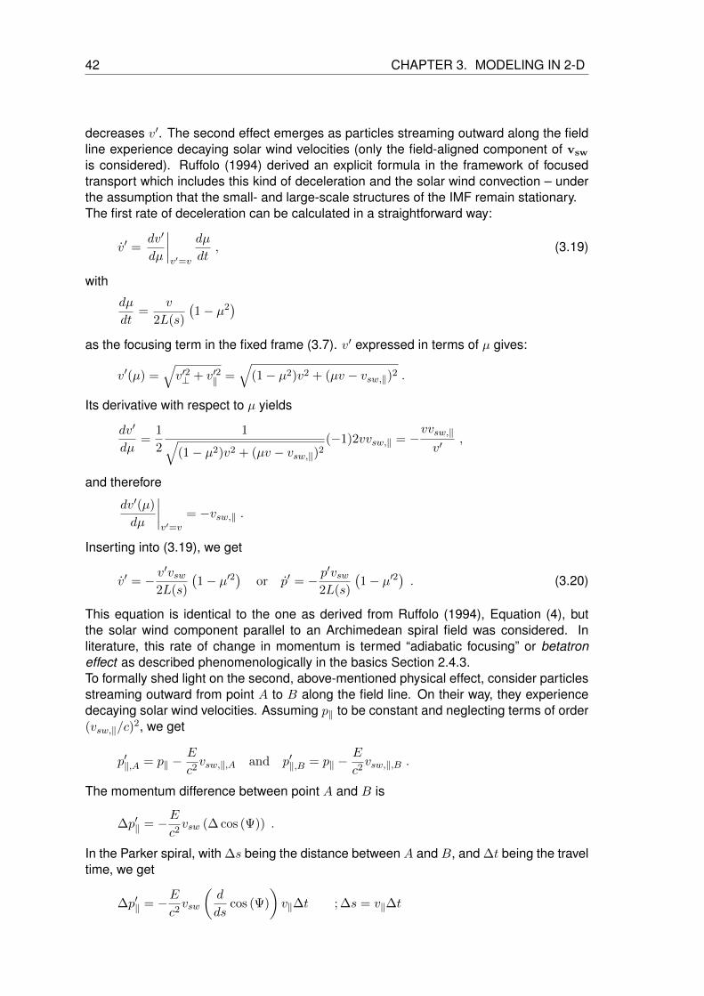
42 CHAPTER 3. MODELING IN 2-D
decreases v′. The second effect emerges as particles streaming outward along the fieldline experience decaying solar wind velocities (only the field-aligned component of vsw
is considered). Ruffolo (1994) derived an explicit formula in the framework of focusedtransport which includes this kind of deceleration and the solar wind convection – underthe assumption that the small- and large-scale structures of the IMF remain stationary.The first rate of deceleration can be calculated in a straightforward way:
v′ =dv′
dµ
∣∣∣∣v′=v
dµ
dt, (3.19)
with
dµ
dt=
v
2L(s)
(1− µ2
)as the focusing term in the fixed frame (3.7). v′ expressed in terms of µ gives:
v′(µ) =√v′2⊥ + v′2‖ =
√(1− µ2)v2 + (µv − vsw,‖)2 .
Its derivative with respect to µ yields
dv′
dµ=
1
2
1√(1− µ2)v2 + (µv − vsw,‖)2
(−1)2vvsw,‖ = −vvsw,‖
v′,
and therefore
dv′(µ)
dµ
∣∣∣∣v′=v
= −vsw,‖ .
Inserting into (3.19), we get
v′ = − v′vsw
2L(s)
(1− µ′2
)or p′ = − p
′vsw2L(s)
(1− µ′2
). (3.20)
This equation is identical to the one as derived from Ruffolo (1994), Equation (4), butthe solar wind component parallel to an Archimedean spiral field was considered. Inliterature, this rate of change in momentum is termed “adiabatic focusing” or betatroneffect as described phenomenologically in the basics Section 2.4.3.To formally shed light on the second, above-mentioned physical effect, consider particlesstreaming outward from point A to B along the field line. On their way, they experiencedecaying solar wind velocities. Assuming p‖ to be constant and neglecting terms of order(vsw,‖/c)
2, we get
p′‖,A = p‖ −E
c2vsw,‖,A and p′‖,B = p‖ −
E
c2vsw,‖,B .
The momentum difference between point A and B is
∆p′‖ = −Ec2vsw (∆ cos (Ψ)) .
In the Parker spiral, with ∆s being the distance between A and B, and ∆t being the traveltime, we get
∆p′‖ = −Ec2vsw
(d
dscos (Ψ)
)v‖∆t ; ∆s = v‖∆t

3.2. AN EXTENDED AND MODIFIED MODEL VERSION 43
⇔ p′‖ = lim∆t→0
∆p′‖(t)
∆t= −p‖vsw
[dr
ds
d
dr(cos (Ψ(r)))
]= −p‖vsw
[cos (Ψ(r))
d
dr(cos (Ψ(r)))
]
⇔ p′‖ = −p‖vsw
1√1 +
(ωrvsw
)2·
− r(ωvsw
)2
(1+( ωrvsw)2)
32
= −p‖vsw
− r(ωrvsw
)2
(1 +
(ωrvsw
)2)2
In order to examine differential convection alone, p′⊥ is fixed. Since p‖vsw ≈ p′‖vsw to firstorder in (vsw,‖/c) – according to Equation (6) in Ruffolo (1994) – the second order rate ofdeceleration is:
p′ =p′‖
p′p′‖ = −p′vsw
(cos (Ψ)
d
dr(cos (Ψ))
)µ′2 (3.21)
The term differs from the former one by the last cosine of Ψ, since another transformationof the solar wind has been made. Under the assumption of isotropic distributions of solarcosmic rays and a radial field, (3.21) simplifies to
< p′ >= −p′
3∇vsw , (3.22)
which has been used in many studies of cosmic ray transport (e.g. Parker, 1965).Finally, the momentum dependent part of Fokker-Planck equation (3.18)with (3.20) and(3.21) becomes:
∂F (t, µ′, s, p′)
∂t=
∂
∂p′
(p′vsw
[cos (Ψ)
2L(s)(1− µ′2) + cos Ψ
∂
∂r(cos (Ψ))µ′2
]F (t, µ′, s, p′)
).
(3.23)
For the sake of completeness, it should be emphasized that, in contrast to the betatroneffect, the inverse Fermi-effect can cool SEPs propagating perpendicular to the field – inparticular around 1 AU, since changes of the field-perpendicular component of the solarwind speed are maximum there. If both field-parallel and perpendicular solar wind effectare considered, it can be denoted as inverse Fermi-effect (Section 2.4.3).
3.2.2. Choice of the grid
We adopted both the Roelof’s Equation and the Ruffolo’s Equation to accommodatecross-field transport in the inner heliosphere. The differential terms are discretized byfinite differences (see Chapter 4), thus the spatial domain of the ecliptic has to be dis-cretized, too: An appropriate grid has to be defined.
Azimuthal Transport
The original one-dimensional code works on equidistant grid points along the magneticfield line with step size ∆s. Expanding this approach to two dimensions combined withazimuthally aligned cross-field trajectories, leads to concentric rings which get closer andcloser to each other with increasing radial distance (see also Lampa and Kallenrode,2009). Thus particles are shifted in the azimuthal direction by
ds⊥(r) = rdϕ. (3.24)

44 CHAPTER 3. MODELING IN 2-D
Figure 3.1.: Perpendicular paths in a grid of azimuthal cross-field transport (∆s = const.).The resulting numerical scheme would be inaccurate since the topology is notsquared – some of the grid points do not contribute to the transport.
But in this spatially fixed frame, these trajectories are just “roughly” perpendicular to theIMF very close to the Sun (within a radius of a few tens of an AU).Consequently, the first step was to find a scheme that would realize perpendicular trans-port without changing the grid architecture. The idea was to calculate the intersectionbetween the perpendicular path with the neighboring field line. In general, these inter-sections are not expected to hit a neighboring grid point exactly (indicated by the blackfilled circles in Figure 3.1). Based on these “virtual grid points”, a weighting factor couldbe established. During cross-field transport, it determines the fractions of particles thatare assigned to the left neighboring grid points (on the same field line like the intersectionpoint) and to the neighboring right points (these are equally colored in Figure 3.1). So,basically, the fluxes in westward/ eastward direction are split into 2 components.Despite this splitting, we can still realize perpendicular transport as essentially one-dimensional - denoted by the point (j, l) in the Figure: The classical diffusion finite dif-ference (FD) needs three neighboring grid point to approximate the second derivative.Here, due to the splitting, six points are involved for each virtual grid point. As an ex-ample, we have marked these inter-point-relationships at point (j, l). This would lead toan equation system that – in matrix form – would have six diagonals (six grid points areinvolved as seen in Figure 3.1), but just under the assumption that the numerical valuesξ of the distribution function are properly arranged within the solution vector vn.
Example for the magenta colored curve:
Avn+1 = vn with vn = (ξ9,6, ξ8,6, ξ8,5, ξ7,5, ξ7,4, ξ6,4, ξ6,3, ξ5,3, ξ5,2, ξ4,2, ξ4,1)T
The sequence of indexes for vn has to be computed before the numerical scheme starts.The sequence differs with respect to different perpendicular curves. If we hit the gridpoints exactly, the resulting matrix A would be tri-diagonal. The equation could be solvedin linear runtime. In case of the six-point-scheme, the effort doubles.In a slightly modified approach, we do not try to solve the complete scheme within a singletime step, but split into an azimuthal part and a part hitting the neighboring (right) point.

3.2. AN EXTENDED AND MODIFIED MODEL VERSION 45
Unfortunately, sometimes and especially at larger radial distances from the Sun and forlarge azimuthal distances ∆ϕ, this fails completely, since the azimuthal part and/or theneighboring part is missing. Starting at point (5, 1) for example, point (5, 2) in azimuthaldirection does not account for cross-field transport.Coming back to the first approach, another artifact can be observed – denoted by thesquares: Further out, where the perpendicular curves tend to point in radial direction,some grid points are never hit, thus there exists no perpendicular transport. On theother hand, there are grid points which are considered twice (or even higher in easterndirection). These cells dry out by trend, although the net flux is kept in balance by theweighting factors. The reason is that the next time step can not be computed for allperpendicular curves simultaneously. We have to prioritize a curve over another.Consequently, the next step was to realize exact perpendicular transport in the plane ofthe ecliptic, where a grid point exactly hits the neighbor during the cross-field shift.
Exact Perpendicular Transport
Figure 3.2.: IMF and perpendicular curves for azimuthal distances of dϕ = 20.
The question now is how to calculate a grid consisting of both the fictitious Archimedeanfield lines and the curves perpendicular to it.The intersections “field line – perpendicular trajectory” can be found by looking at thelocal geometry in Figure 3.3: The dotted curves of lower density indicate two field lineswithin the ecliptic plane, originating at the Sun S. The intersection point A of the denselydotted, perpendicular curve is known by construction. The following intersection point Bcan be found by calculating the slope triangle in point (r0, 0):
rdϕ
dr=
cos (Ψ(r))ds⊥sin (Ψ(r))ds⊥
,
where ds⊥ denotes an infinitesimal deviation in field-perpendicular direction. Simplifying
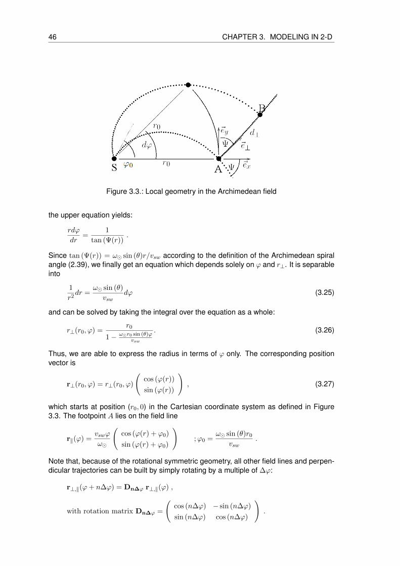
46 CHAPTER 3. MODELING IN 2-D
Figure 3.3.: Local geometry in the Archimedean field
the upper equation yields:
rdϕ
dr=
1
tan (Ψ(r)).
Since tan (Ψ(r)) = ω sin (θ)r/vsw according to the definition of the Archimedean spiralangle (2.39), we finally get an equation which depends solely on ϕ and r⊥. It is separableinto
1
r2dr =
ω sin (θ)
vswdϕ (3.25)
and can be solved by taking the integral over the equation as a whole:
r⊥(r0, ϕ) =r0
1− ωr0 sin (θ)ϕvsw
. (3.26)
Thus, we are able to express the radius in terms of ϕ only. The corresponding positionvector is
r⊥(r0, ϕ) = r⊥(r0, ϕ)
(cos (ϕ(r))
sin (ϕ(r))
), (3.27)
which starts at position (r0, 0) in the Cartesian coordinate system as defined in Figure3.3. The footpoint A lies on the field line
r‖(ϕ) =vswϕ
ω
(cos (ϕ(r) + ϕ0)
sin (ϕ(r) + ϕ0)
);ϕ0 =
ω sin (θ)r0
vsw.
Note that, because of the rotational symmetric geometry, all other field lines and perpen-dicular trajectories can be built by simply rotating by a multiple of ∆ϕ:
r⊥,‖(ϕ+ n∆ϕ) = Dn∆ϕ r⊥,‖(ϕ) ,
with rotation matrix Dn∆ϕ =
(cos (n∆ϕ) − sin (n∆ϕ)
sin (n∆ϕ) cos (n∆ϕ)
).

3.2. AN EXTENDED AND MODIFIED MODEL VERSION 47
The Archimedean field lines are defined for all ϕ, but the perpendicular trajectories endasymptotically in radially outward directed lines (see Figure 3.2). That is the reason why(3.27) – starting at ϕ = 0 is only valid for longitudes ϕ ∈ [0, vsw
ω sin (θ)r0[.
Using Pythagoras’ theorem, one can easily derive the arc length of the perpendicularcurves needed to compute the distances between the field lines:
ds⊥ =√dx2 + dy2 =
√(dx(r0, ϕ)
dϕ
)2
+
(dy(r0, ϕ)
dϕ
)2
dϕ .
With x(r0, ϕ) = r⊥(r0, ϕ) cos (ϕ) and x(r0, ϕ) = r⊥(r0, ϕ) sin (ϕ), ds⊥ can be reformulatedaccording to the azimuth ϕ:
ds⊥ =
√(dr(ϕ)
dϕ
)2
+ (r(ϕ))2dϕ =
√(r⊥(ϕ)2ω sin (θ)
vsw
)2
+ r⊥(ϕ)2 dϕ .
A step size along a curve (or arc length) perpendicular to the IMF implies a change inazimuth of ∆ϕ, which is denoted by the longitudinal distance between two neighboringfield lines.For simplicity (and without loss of generality) we assume that the perpendicular trajecto-ries are drawn in the ecliptic plane with θ ≈ 90. We can integrate the expression above:
∆s⊥(r0,∆ϕ) =
∫ ϕ(r0)+∆ϕ
ϕ(r0)
√(r⊥(ϕ)2ω
vsw
)2
+ r⊥(ϕ)2 dϕ.
This is the perpendicular distance between two field lines. The integration path startsat radius r0, positive values in ϕ indicate westward (anti-clock-wise) and negative valueseastward direction.
ds⊥(r0,∆ϕ) =vsw
ωχ(r0, ϕ)
[−χ(r0, ϕ) log
(2
(−χ(r0, ϕ) +
√(r2
0ω2 + χ(r0, ϕ)2)
))−√χ(ϕ)2 + r2
0ω2
]∣∣∣∣ϕ(r0)+∆ϕ
ϕ(r0)
(3.28)
with
χ(r0, ϕ) = r0ϕω − vsw .
By doing so, we have overcome the problem from Jahns (2007) who actually found ade-quate perpendicular distances ds⊥(r) = rdϕ/(1 + tan (Ψ(r))2) by linear approximation.As it is seen in Figure 3.4, ds⊥(r) is underestimated to the west of the correspondingfield line in the Jahns’ approach, and overestimated when going westward – owing to thelinear approach.Very close to the Sun ds⊥(ϕ(r)) increases almost linearly with ds⊥ ∝ rdϕ (indicated bythe dotted line), since the field lines are aligned in radial direction (well in agreement withazimuthal transport and the Jahn’s approach). The values coincide beyond a few AU aswell, due to the concentric rings forming field lines whose corresponding perpendicular

48 CHAPTER 3. MODELING IN 2-D
0 2 4 6 8 100
0.1
0.2
0.3
0.4
0.5
0.6
0.7
0.8
r [AU]
ds ⊥
(r)[AU]
ds⊥(r) in western direction
ds⊥(r) in eastern direction
ds⊥(r) = rdϕ cos (Ψ), Jahns approach
ds⊥(r) = rdϕ in radial geometry
upper boundary ds⊥,max = dϕvsw/ω⊙
Figure 3.4.: Perpendicular distance ∆s⊥(r) between two neighboring field lines for ∆ϕ =45 (angular distance between 2 field lines.)
Figure 3.5.: The hybrid grid as a combination of both concentric rings close to the Sunand perpendicular trajectories.

3.2. AN EXTENDED AND MODIFIED MODEL VERSION 49
Figure 3.6.: Reducing the azimuthal extent of the perpendicular grid.
curves are directed in the radial direction. For these geometrical reasons, ds⊥(r) reachesasymptotically the upper boundary ∆s⊥,max = ∆ϕvsw/ω.During the time ∆T , a field line has been wound up once by
∆ϕ = ω∆T.
At the same time, is has been shifted in radial direction by the increment
∆r = vsw∆T.
Since ∆r = limr→∞∆s⊥(r) = ∆s⊥,max we finally get the maximal perpendicular distanceas mentioned above.The values of this current approach and the one of Jahn differ the most at 1 AU (theEarth’s orbit) where the spiral angle is Ψ ≈ 45. These differences seem to be not thatmuch – especially for ∆ϕ→ 0. But local errors sum up when the perpendicular paths arecalculated incrementally, by going from one field line to the neighboring one, calculatingthe intersections of the perpendicular curve and the neighboring field line.

50 CHAPTER 3. MODELING IN 2-D
Since we know about the intersections between the field lines and their perpendicularcounterparts, as expressed by r⊥(r0, ϕ) in (3.26), we can compute the field parallel dis-tance between two intersection points: The neighboring radii, denoted by
r⊥(r0, ϕn) and r⊥(r0, ϕn+1) with ϕn+1 = ϕn + n∆ϕ ;n ∈ N ,
are transformed into the corresponding arc length along the field line by applying (2.39)and then taking the difference. For a fixed position, the parallel step sizes ∆s‖(r) areeven smaller than ∆s⊥(r) – as it also can be seen in Figure 3.2. In the numerics section4.2 at (4.21), it will be shown that very low values of ∆s‖ enlarge the computation time ofthe numerical model significantly.This negative effect can be weakened by introducing some restrictions to the grid. Prob-ably the most effective technique would by a “hybrid” approach, which combines both thefeatures of the purely azimuthal grid and the perpendicular grid (see Figure 3.5). Thevery inner region below r = 0.05 AU is replaced by concentric rings. The distance be-tween two neighbouring rings is given by the smallest ∆s‖ (red colored line, indicated byan arrow in Figure 3.5). If that region of concentric rings had been covered by perpen-dicular trajectories, ∆s‖ would be significantly smaller. A negative, secondary effect arevery large step sizes in the transition region between the azimuthal and perpendiculardomain. The hybrid approach has not been implemented yet, but at least one featurecan already be applied: The more the inner boundary is shifted Sun outward, the largerthe step sizes will be. Unfortunately, by doing so, the domain close to the Sun will notbe covered anymore. In order to still simulate close to the Sun and simultaneously haveadequate step sizes, we could reduce the azimuthal extent around the CFL instead, asindicated in Figure 3.6. The smallest step sizes are found at the eastern boundary. Theless we are forced to go westward, the larger are the step sizes. Note that this is the mostuseful method if it is a priori known that no significant particle populations reach the theouter boundary within the simulation period.
To sum up, Ruffolo’s equation has been applied within the plane of ecliptic by introducinga second spatial coordinate s⊥ perpendicular to the field. The frame of reference hasbeen changed to the field-parallel component of the solar wind speed. The resulting gridis used in the following chapter to solve the transport equation numerically.

4. Numerics in Non-equidistant Grids
The goal is to build a numerical scheme that can adequately approximate the solution ofthe transport equation (3.9). As we know, an exact analytical solution is possible undervery strong simplifications only see also (see also Hatzky, 1996; Lampa, 2006).Fortunately, we are able to adopt (at least in some parts) the Finite Difference (FD)schemes which have been applied to Roelof’s (1969a) and later also to Ruffolo’s equation(1994) on equally spaced grids by Wong (1982), Schluter (1985), Ruffolo (1994), Hatzky(1996) and others.
4.1. Basics of the Finite-Difference Method
The infinite set of values in the continuous solution F is represented by a finite set ofvalues ξ referred to as the discrete solution. For simplicity, we consider first the case ofa function ξ of two variables t and x (time and space coordinate). Given a set of pointsxi; i = 1, . . . , I and tn;n = 1, . . . , N in the domain of F(t,x), the numerical solution isrepresented by a discrete set of function values ξn,i|; i = 1, . . . , I;n = 1, . . . , N thatapproximate F at these points, i.e., ξn,i ≈ F (tn, xi). For a better comprehension, thepoints are assumed to be equally spaced within the domain with constant step sizes∆t = tn+1 − tn; n = 1, . . . , N − 1 and ∆x = xi+1 − xi; i = 1, . . . ; I − 1.
4.1.1. Consistency of finite differences
The construction of the numerical scheme involves the replacement of the differentialterms by the corresponding finite difference (FD) terms. The latter ones can be build byusing Taylor expansions around the point tn or xi. For instance, the forward differenceapproximation gives to ξi+1 ≈ F (xi+∆x) using N+1 terms of a Taylor expansion aroundxi is given by
ξi+1 = ξi + ∂x F (x)|x=xi∆x+ ∂xx F (x)|x=xi
∆x2
2+ · · ·
+∂n
∂nxF (x)|x=xi
∆xn
n!+∂n+1
∂n+1x
F (x∗)|x=xi
∆xn
(n+ 1)!. (4.1)
The last term is called the remainder with xi ≤ x∗ ≤ xi+1, and represents the error inthe approximation if only the first n terms in the expansion are considered. Although theexpression (4.1) is exact, the position x* is unknown.Putting ξi on the left side of (4.1) and dividing by ∆x, we obtain the forward differenceapproximation of ∂F
∂x
∣∣x=xi
:
∂F
∂x
∣∣∣∣x=xi
=xi+1 − xi
∆x+ εi ,
where εi is given by
εi = −∆x
2∂xxF (x∗) +O((∆x)2) .
51

52 CHAPTER 4. NUMERICS IN NON-EQUIDISTANT GRIDS
Alternative approximations such as the backward and centered FD approximations (Chat-tot, 2002, p.6), would be also mathematically equivalent to the forward difference term:The approximations converge towards the derivative as ∆x → 0. But since ∆x is finite,the numerical solutions of different FD converge differently towards the exact solution,which is indicated by the truncation error εi.
The truncation error is defined as the difference between the exact value and its numericalapproximation. This term depends on ∆x but also on F and its derivatives. The order ofa finite difference approximation in terms of the step size is defined as the power p suchthatlim
∆x→0(ε/∆xp) = γ 6= 0, where γ is a finite value. This is often written as εi = O(∆xp).
For instance, the forward difference approximation gives εi = O(∆x) and it is said to befirst-order accurate (p = 1).If we apply this method to the centered finite difference approximation, we find that, forconstant ∆x, their errors are
∂F
∂x
∣∣∣∣x=xi
=xi+1 − xi−1
2∆x− ∆x2
12∂xxxF (x∗) → εi = O(∆x2) .
The εi will be separately computed for each variable, keeping the other variable t con-stant. In the overall numerical scheme, the truncation errors for each FD will be added,e.g. εni = εi + εn.The resulting scheme has to be consistent which means that the truncation error εni(difference between the differential and its discretized terms) with respect to independentvariable xi and time tn has to converge towards zero if the corresponding step sizes goto zero.
4.1.2. Stability
Having a stable numerical scheme requires that inherent, initial perturbations of the FDscheme are not allowed to grow arbitrarily high. The discrete solutions ξni have to bebounded within the domain:
ξni ≤ C(∆t,∆x, ξ0(t = t1, 0), ξ1(t, x = x1), ξ2(t, x = xI)) ∀ i = 1, . . . , I . (4.2)
The constant boundary C depends on the step sizes as well as the initial value ξ0 and theboundary conditions ξ1, ξ2. The inequality (4.2) originally comes from the treatment of theFDE as a Cauchy problem (Samarskij, 2001, p. 384). Assuming that the discrete solutionis separable with respect to the time, the scheme can be rewritten as a linear equationsystem ξ(n+1) = Aξ(n) that iteratively describes the temporal evolution of ξi; i = 1, . . . , Ifrom tn to tn+1. Special requirements to A, n-times application of the linear equationsystem, starting at t = t1 and a proper choice of the norm would give an estimate of theupper boundary, denoted by (4.2).If a limiting upper boundary is needed according to the maximum norm ‖ξni ‖max =maxi |ξi|, this would lead to the application of the maximum principle (Samarskij, 2001,p. 258), which is equivalent special properties of the matrix A. We will come back to thedetails of stability analysis in the following sections, especially in Section 4.5.2. Matrixeigenvalues analysis in this context would be an alternative approach, but there are moreinvolved.

4.1. BASICS OF THE FINITE-DIFFERENCE METHOD 53
Another norm under consideration is the euclidean norm
‖ξni ‖2 =((ξn1 )2 + (ξn2 )2 + · · ·+ (ξnI )2
)1/2.
Unfortunately, because of its averaging nature, highly frequent parts of ξ – high valuesof single components ξ(n)
i according to amount – will be damped, which might lead tounreasonable, high or even negative discrete solutions.The stability of FD schemes for hyperbolic and parabolic PDEs under the Euclidean normcan be analyzed by the Von Neumann (or Fourier) method. It can only be applied tolinear homogeneous FD equations or systems, as it is based on the superposition ofwave modes. The idea behind the method is the following: The analytical solutions ofe.g. the model diffusion equation ∂tF (t, x)− b∂xxF (t, x) = 0 can be found in the form
F (t, x) =∞∑m=0
∞∑l=0
gm exp (βmt) exp (iklx) ;
with wave numbers kn and frequency βm of mode m, as it shown e.g. in (Chattot, 2002,p.54). This solution involves a Fourier series in space and an exponential decay intime since βm ≤ 0. Here we have included the complex version of the Fourier series,exp (iklx) = cos (klx) + i sin (klx) with the imaginary unit i =
√−1, because this consid-
erably simplifies later algebraic manipulations. To analyze the growth of different Fouriermodes as they evolve under the numerical scheme we can consider each mode sepa-rately, namely
Fm,l(t, x) = gm exp (βmt) · exp (iklx) .
A discrete version of this equation is ξ(n)i = gm exp (βmtn) exp (iklxj). We can use, without
loss of generality and in case of equally spaced grid points, xj = j∆x and tn = n∆t toobtain
ξ(n)j = gnm exp (βmn∆t) · exp (iklj∆x) = exp (βm∆t)n · exp (iklj∆x) .
The term exp (iklj∆x) = cos (klj∆x)+i sin (klj∆x) is bounded and, therefore, any growthin the numerical solution will arise from the complex amplitude raised to the n-th powergnm. Each Fourier mode is treated separately: The linearity of the equations insuresthat, if the numerical scheme is stable for each mode, it will be stable for any superpo-sition of modes. Putting the complex Fourier mode into the FD equation and dividing bygnm exp (βmn∆t) yields the amplification factor gm. The numerical method will be stableand the numerical solution F
(n)i will be bounded with n → ∞ respectively, if |gm| ≤ 1.
Stability analysis, using the Von Neumann method, of implicit as well as explicit diffusionscheme can be found in literature or e.g. in Lampa (2006).
Then, if both characteristics (consistency and stability) are fulfilled, the PDE is said to beconvergent according to the Lax’s equivalent-theorem (see Richtmyer and Morton, 1967).
4.1.3. Summarized approximation method
Within the overall numerical scheme, the distribution function F depending on momentumpk and pitch-cosine µi at location (s‖,j , s⊥,l) at time tn will be denoted by its numericalvalue ξnj,l,i,k.

54 CHAPTER 4. NUMERICS IN NON-EQUIDISTANT GRIDS
The time derivative will be discretized by the forward difference
∂F
∂t
∣∣∣∣t=tn
=ξn+1 − ξn
∆t+O(∆t) , (4.3)
which is accurate to first order in constant step size ∆t. Additionally, if all terms in a partialdifferential equation (PDE) can be linearized (as it is done in this study), the resultingdifference scheme can be expressed by a matrix form – even if ξ depends on more thanone independent variable (see Samarskij, 2001). The operator A(n+1) with all entriesaccording to time tn+1 has to be limited by a finite upper boundary (this always true forlinear PDEs) and A(n) has to be at least diagonal dominant. Consequently, the inverse ofA(n) exists and the next time step can be executed by solving the linear equation system.In general, the system matrix M =
(A(n)
)−1A(n+1) will not be “well shaped”. There will
exist many entries beyond the main diagonal and they are not expected to uniformly fillthe secondary diagonals with non-zero values. There would be many clusters of non-zerovalues and the system matrix would not be symmetric.The Gaussian elimination method will be in the order of O(m2) - with m = ls · lµ · lz · lpbeing the row/ column number of M. The l variables correspond to the number of gridpoints within the s‖, µ, s⊥, and p domain. Comparing to the computational possibilitiesat present, this leads to an unacceptable runtime. But apart from that, one would prob-ably fail at taking the hurdle to invert A(n). The diagonal dominance is a strong stabilityrestriction as we will see later on.So, again, we adopted the numerical scheme described by Hatzky (1996). Its basis isan enhanced fractional time step and time splitting method (e.g. Marchuk, 1975) – alsoknown under summarized approximation method (see Samarskij, 2001) - which allows totreat transport in each independent variable separately, reducing this multi-dimensionalproblem to a chain of one-dimensional problems. As nomenclature, all properties, that donot change during a specific transport, are not indicated. For instance, in case of pitch-angle transport, all spatial variables and momentum will be left out, and the numericalrepresentant of F reads ξni . Splitting in two half steps and arranging each separate,pairwise occurring scheme in s‖, s⊥, µ and p in a symmetric manner increases overallapproximation in time to second order. In simple words: During each time step, spatials‖-transport is advanced by half a step, pitch-angle transport is advanced by half a step,perpendicular transport is advanced by half a step, momentum transport happens in twohalf steps, perpendicular transport is advanced by the second half a step, pitch-angletransport is advanced by the second half step and finally spatial s‖-transport is advancedby the second half step.The difference operator for the µ-transport e.g. is written Lµ(t, s‖, s⊥, µ, p) and the otherfour are accordingly defined. The overall consistency and stability of the overall scheme
L(t, s‖, s⊥, µ, p) =
1
2Ls‖(t, s‖, s⊥, µ, p) +
1
2Lµ(tn, s‖, s⊥, µ, p) +
1
2Ls⊥(t, s‖, s⊥, µ, p) +
1
2Lp(t, s‖, s⊥, µ, p)
+1
2Lp(t, s‖, s⊥, µ, p) +
1
2Ls⊥(t, s‖, s⊥, µ, p) +
1
2Lµ(tn, s‖, s⊥, µ, p) +
1
2Ls‖(t, s‖, s⊥, µ, p)
is determined by the sum of stability criteria and consistencies for each seperate differ-ence scheme in t, s‖, s⊥, µ and p.To have symmetric a scheme, which is split into two temporal half-steps, allows eachtransport process to be nearly equally represented in the overall framework. But notethat the first executed transport is always more dominant than the others.

4.2. TRANSPORT ALONG AN IMF LINE (S-TRANSPORT) 55
Whereas the simplified, azimuthal grid is based on a constant step size ∆s along themagnetic field line (see Section 3.2.2), we now have to take care of possible restrictionsusing varying step sizes. The numerical grid is based on the geometry we have definedin Section 3.2.2.
Building an expanded model on a distorted grid forces the developer to pay attentionto the correct assignment of array indexes. Unlike the former 2-D model (Lampa andKallenrode, 2009), one single step in the cross-field direction results in both a change inazimuth and radial distance. In order to make the architecture more clear, the schematicspatial grid in Figure 4.1 might help to get an overview. Note that this grid just describesthe topology, and not exact distances between two neighboring points. This dependsstrongly on the radial distance.
Figure 4.1.: Schematic grid including some variables of the numerical model nperpgref.The field lines are aligned horizontally.
The simulated particles are injected on the footpoint of the central field line (CFL) via adelta-function, or even more extended symmetrically around the CFL (see Section 4.6).The footpoints are located at s⊥,ml with ml = blz/2 + 1c. Note that – according to thenotation in Figure 4.1 – the CFL does not start at s1 but at sml.
Summing up, this subsection provides a short introduction into solving partial differentialequations numerically via finite differences – in particular for varying step sizes. Thesummarized approximation method is applied for this multi-dimensional problem.
4.2. Transport along an IMF line (s-transport)
The second order finite difference scheme, that has been derived by Lax-Wendroff (An-derson et al., 1984), will be maintained in its structure for field-parallel transport. Hatzkyalready illustrated that this second order accurate FD scheme combined with a monotoni-zed-centered flux-limiter (van Leer, 1977) would be the best choice. According to the

56 CHAPTER 4. NUMERICS IN NON-EQUIDISTANT GRIDS
Courant-Friedrichs-Levy (CFL) stability condition
γ = maxj,i|vj,i|
∆t
∆s‖≤ 1 , (4.4)
the step sizes are chosen such that the scheme works exactly for the fastest particles.We preferred this scheme over the first-order-upwind scheme as well as over the flux-corrected transport (numerical artefacts/ terraces at strong gradients for γ << 1). But wehave to address the question whether the varying step sizes pose additional problems/restrictions to the numerical code.As we remember, the Lax-Wendroff-scheme was built by making a Taylor expansionaround a certain point in time tn and by replacing the resulting time derivatives by thecorresponding space derivatives which are defined by the hyperbolic differential equationitself:
∂F
∂t+ v
∂F
∂s‖= 0 ; v particle speed . (4.5)
Again, let ξnj be the numerical value of the analytical, PDE solving function F at point(tn, s‖,j). The Taylor expansion around tn yields:
ξ(t+ ∆t, s‖,j) = F (t, s‖,j) + ∆t∂tF (tn, s‖,j) +1
2∆t2∂ttF (tn, s‖,j) +O(∆t3) .
Replacing the time derivatives using equation (4.5) and ignoring higher order terms weget another formulation of the advection equation
∂F
∂t= −v ∂F
∂s‖+
∆t2
2
∂2F
∂s2‖, (4.6)
which has already been solved numerically for equispaced step sizes ∆s‖. The additionaldiffusion terms prevents the numerical solution to be smeared out less with time thanwithout the diffusion term (numerical diffusion, see e.g. Roach, 1982). The first derivativein s is chosen to be the centered finite-difference approximation and the second derivativeis set to be the conventional second order difference scheme well known in terms ofa numerical solution of the one-dimensional heat equation. Hatzky (1996) and othersalready incorporated the case of spatially varying velocities.The final result can be found at p. 54:
ξn+1j = ξnj −
(γj+1/2ξ
nj − γj−1/2ξ
nj−1
)− ηj+1/2(ξnj+1 − ξnj ) + ηj−1/2(ξnj − ξnj−1) , (4.7)
with γj+1/2 = vj+1/2∆t
∆s‖and ηj+1/2 = 1
2γj+1/2(1− γj+1/2).
This scheme is second order accurate and saves monotony (Roe, 1986), or in otherwords: spatial distributions of ξ do not change local slope sign during the entire sim-ulation. Of course, exceptions from the monotony feature are additional sources suchas modeled traveling shocks or SEPs originating from a different flare/ CME that is notmagnetically connected to the observer’s field line. Resuming the numerics, we can alsostate that the stability criterion is identical to the one in case of the much simpler Eulerianscheme (Courant-Friedrichs criterion, for short: CFL).

4.2. TRANSPORT ALONG AN IMF LINE (S-TRANSPORT) 57
This scheme prevents particles to get lost out of the system by applying the control vol-ume approach (Roach, 1982) which insures that all particles leaving a certain cell arecompletely transported to one or more neighboring cells.The scheme mentioned above does not work anymore when spatial step sizes becomevariable. With regard to the calculated IMF grid we are dealing with increasing stepsizes as particles are transported from the Sun outwards along the local field line and asparticles are swept westward along a perpendicular path respectively.
Fl+ 12
t tt t t - -
-
- -zl−2 zl−1 zl zl+1 zl+2
∆zl−1 ∆zl
z
Fl− 12
t
Figure 4.2.: Grid structure in both field-parallel (s‖-) and field-perpendicular (s⊥-)direction.
Based on the grid, as denoted by Figure 4.2, the following scheme can be applied tovariable particle speeds and step sizes as well:
ξn+1j = ξnj −∆t
[(vj+1/2
ξnj+1 + ξnj2
− vj−1/2
ξnj + ξnj−1
2
)/
(∆s‖,j−1 + ∆s‖,j
2)
)]+
∆t2
2
[(v2j+1/2
ξnj+1 − ξnj∆s‖,j
− v2j−1/2
ξnj − ξnj∆s‖,j−1
)/
(∆s‖,j−1 + ∆s‖,j
2
)].(4.8)
Again, we made an adoption of the control volume approach. Unknown values at the cellboundaries (here: particle velocity) were calculated by arithmetic means.The first term in square brackets (4.8) numerically describes the advective in- and outputsF at cell s‖,j .
v‖(s‖)∂f
∂s‖
∣∣∣∣s‖=s‖,j
≈Fj+1/2 − Fj−1/2
∆s‖,j−1+∆s‖,j2
with Fj+1/2 = v‖,j+1/2
ξnj+1 + ξnj2
. (4.9)
Remember that this centered finite difference approximation is not accurate to secondorder but to first order only. Its consistency can be proven by putting the exact, Taylor-expanded solution F (s‖) into the FD in place of the approximated solution:
v‖,j+1/2ξnj+1+ξnj
2 − v‖,j−1/2ξnj +ξnj−1
2∆s‖,j−1+∆s‖,j
2
=F (s‖,j)
∆s‖,j−1 + ∆s‖,j(v‖,j+1/2 − v‖,j−1/2) (4.10)
+v‖,j−1/2∆s‖,j−1 + v‖,j+1/2∆s‖,j
∆s‖,j−1 + ∆s‖,j
∂F
∂s‖(4.11)
+1
2
v‖,j−1/2∆s2‖,j−1 + v‖,j+1/2∆s2
‖,j
∆s‖,j−1 + ∆s‖,j
∂2F
∂s2‖
(4.12)
+ O(∆s3‖,j−1 + ∆s3
‖,j) .

58 CHAPTER 4. NUMERICS IN NON-EQUIDISTANT GRIDS
It should be noted that particle velocities v‖(s‖) and ∆s‖(s‖) have to be continuously dif-ferentiable functions in s‖. v‖,j−1/2 and v‖,j+1/2 become identical when the cell boundariesconverge asymptotically.The limiting values can be determined by also making a Taylor expansion for the velocitiesaround s‖,j , neglecting terms higher than first order:
v‖,j+1/2 = v‖,j +∆s‖,j
2
∂v‖(s‖)
∂s‖
∣∣∣∣s‖=s‖,j
and v‖,j−1/2 = v‖,j−∆s‖,j−1
2
∂v‖(s‖)
∂s‖
∣∣∣∣s‖=s‖,j
.
The first term on the right-hand site of (4.10) becomes:
F (s‖,j)
∆s‖,j−1 + ∆s‖,j(v‖,j+1/2 − v‖,j−1/2) =
1
2F (s‖)
∂v‖(s‖)
∂s‖
∣∣∣∣s‖=s‖,j
(4.13)
Analogous to this term, the following two terms (4.11) and (4.12) are further approximatedto:
v‖,j−1/2∆s‖,j−1 + v‖,j+1/2∆s‖,j
∆s‖,j−1 + ∆s‖,j
∂F
∂s‖= v‖(s‖)
∂F (s‖)
∂s‖
∣∣∣∣s‖=s‖,j
(4.14)
+∆s2‖,j−1 + ∆s2
‖,j
∆s‖,j−1 + ∆s‖,j
∂v‖(s‖)
∂s‖
∂F (s‖)
∂s‖
∣∣∣∣s‖=s‖,j
(4.15)
and
1
2
v‖,j−1/2∆s2‖,j−1 + v‖,j+1/2∆s2
‖,j
∆s‖,j−1 + ∆s‖,j
∂2F
∂s2‖
=1
2
∆s2‖,j−1 + ∆s2
‖,j
∆s‖,j−1 + ∆s‖,jv‖(s‖)
∂2F (s‖)
∂s2‖
∣∣∣∣∣s‖=s‖,j
(4.16)
+1
4
∆s3‖,j−1 −∆s3
‖,j
∆s‖,j−1 + ∆s‖,j
∂v‖(s‖)
∂s‖
∂2F (s‖)
∂s2‖
∣∣∣∣∣s‖=s‖,j
(4.17)
To achieve a consistent FD approximation, spatial changes of the particles’ velocity haveto be small compared to the local step size ∆s‖(s‖). According to (2.38) the step size∆s‖ is related to the corresponding radial change via
dr =
√1 +
(sin θωr
vsw
)2
ds‖(r) =1
cos (Ψ(r))ds‖(r) .
We therefore get:
d
ds‖(v‖(s‖)) =
d
ds‖
(v′‖ + vsw cos(Ψ(s‖(r)))
)
⇔ cos (Ψ(r))d
dr
(v‖(s‖(r))
)= cos (Ψ(r))
d
dr
(v′‖ + vsw cos (Ψ(r)))
).
For vsw = 400 km s−1 and a solar angular frequency of ω = 0.0103 h−1 within the planeof ecliptic, the particles’s speed in the rest frame of the Sun changes by∣∣∣∣dv‖(s‖(r))ds‖(r)
∣∣∣∣ =
∣∣∣∣− cos (Ψ(r))4 (ωr)2 1
vsw
∣∣∣∣ << 0.0024 . (4.18)
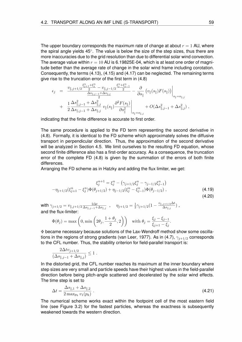
4.2. TRANSPORT ALONG AN IMF LINE (S-TRANSPORT) 59
The upper boundary corresponds the maximum rate of change at about r = 1 AU, wherethe spiral angle yields 45. The value is below the size of the step sizes, thus there aremore inaccuracies due to the grid resolution than due to differential solar wind convection.The average value within r = 10 AU is 6.19825E-04, which is at least one order of magni-tude better than the average rate of change in the solar wind frame including corotation.Consequently, the terms (4.13), (4.15) and (4.17) can be neglected. The remaining termsgive rise to the truncation error of the first term in (4.8)
εj =v‖,j+1/2
ξnj+1+ξnj2 − v‖,j−1/2
ξnj +ξnj−1
2∆s‖,j−1+∆s‖,j
2
− ∂
∂s‖
(v‖(s‖)F (s‖)
)∣∣∣∣s‖=s‖,j
+1
2
∆s2‖,j−1 + ∆s2
‖,j
∆s‖,j−1 + ∆s‖,jv‖(s‖)
∂2F (s‖)
∂s2‖
∣∣∣∣∣s‖=s‖,j
+O(∆s2‖,j−1 + ∆s2
‖,j) ,
indicating that the finite difference is accurate to first order.
The same procedure is applied to the FD term representing the second derivative in(4.8). Formally, it is identical to the FD scheme which approximately solves the diffusivetransport in perpendicular direction. Thus, the approximation of the second derivativewill be analyzed in Section 4.5. We limit ourselves to the resulting FD equation, whosesecond finite difference also has a first-order accuracy. As a consequence, the truncationerror of the complete FD (4.8) is given by the summation of the errors of both finitedifferences.Arranging the FD scheme as in Hatzky and adding the flux limiter, we get:
ξn+1j = ξnj −
(γj+1/2ξ
nj − γj−1/2ξ
nj−1
)−ηj+1/2(ξnj+1 − ξnj )Φ(θj+1/2) + ηj−1/2(ξnj − ξnj−1)Φ(θj−1/2) , (4.19)
(4.20)
with γj+1/2 = v‖,j+1/22∆t
∆s‖,j−1+∆s‖,j, ηj+1/2 = 1
2γj+1/2(1− v‖,j+1/2∆t
∆s‖,j) ,
and the flux-limiter:
Φ(θj) = max
(0,min
(2θj ,
1 + θj2
, 2
))with θj =
ξj − ξj−1
ξj+1 − ξj.
Φ became necessary because solutions of the Lax-Wendroff method show some oscilla-tions in the regions of strong gradients (van Leer, 1977). As in (4.7), γj+1/2 correspondsto the CFL number. Thus, the stability criterion for field-parallel transport is:
2∆tvj+1/2
(∆s‖,j−1 + ∆s‖,j)≤ 1 .
In the distorted grid, the CFL number reaches its maximum at the inner boundary wherestep sizes are very small and particle speeds have their highest values in the field-paralleldirection before being pitch-angle scattered and decelerated by the solar wind effects.The time step is set to
∆t =∆s‖,1 + ∆s‖,2
2 maxpk v1(pk). (4.21)
The numerical scheme works exact within the footpoint cell of the most eastern fieldline (see Figure 3.2) for the fastest particles, whereas the exactness is subsequentlyweakened towards the western direction.

60 CHAPTER 4. NUMERICS IN NON-EQUIDISTANT GRIDS
4.3. Transport in pitch-cosine
This linear, parabolic convection-diffusion equation
∂ξ
∂t+
∂
∂µ(b(µ)ξ)− ∂
∂µ
(κµ(µ)
∂ξ
∂µ
)= 0 , (4.22)
with
b(µ) =1− µ2
2L(s)and κµ(µ) =
3
4
1
λ‖(s)κµ(µ) ,
has been solved according to the following discretization:The focusing term has been approximated by the central difference
∂
∂µ(b(µ)ξ(µ))
∣∣∣∣µ=µi
≈Fi+1/2 − Fi−1/2
∆µwith Fi+1/2 = bi+1/2
ξi+1 + ξi2
,
and the pitch-angle scattering term by the classical second order difference quotient:
∂
∂µ
(κµ(µ)
∂
∂µξ(µ)
)∣∣∣∣µ=µi
≈wi+1/2 − wi−1/2
∆µ; with wi+1/2 = ai+1/2
ξi+1 − ξi∆µ
.
Note that these discrete terms remain unchanged compared to the original code sincewe are still working on an equally spaced grid in µ. The focusing length L(s) and κµ,which both have spatial dependencies, have to be computed with regard to the new grid.The truncation error still gives ε(n)
i = O((dµ)2) for the entire µ-transport.We adopted the implicit, second order scheme since the stability criterion for an explicitscheme
∆t ≤ 1
2
(∆µ)2
κµ(r, µ)(4.23)
would be rather strict (Roach, 1982). Thus, the upper-mentioned difference quotientshave been defined according to the next time step tn+1. If the values of the PADC areexplicitly discrete and have discontinuities (e.g. κµ(µ) at µ = 0 for q = 1 and σ 6= 0)– that is to say, they do not solve a continuous function f : N → R with f(µi) = κµ(µi),κµ(µi±1/2) = ai±1/2 will be determined by the Integro-interpolation-method (Tichonov andSamarskij, 1961) or by linear interpolation.Putting together all difference equations for all i, we get a system of linear equationswhose system matrix reveals a tri-diagonal shape. The diagonal dominance has to befulfilled for stability. This leads to an essential condition for the focusing length (Hatzky,1996, p. 62):
L ≥ ∆τ
(1 +
∆µ
2
). (4.24)
Another restriction emerges from the fact that both µ-terms in the transport equationcompete against each other: Close to the Sun, focusing dominates, whereas beyond afew tens of an AU pitch-angle scattering strongly affects the particle distributions. It hasbeen calculated that
maxi
∣∣∣∣ bi+1/2
ai+1/2
∣∣∣∣∆µ < 2 , ρi+1/2 =bi+1/2
ai+1/2,

4.4. ADIABATIC DECELERATION (MOMENTUM-TRANSPORT) 61
has to be fulfilled to be stable throughout the entire simulation.Additionally, the consistency error ε(n)
i might grow to infinity if κµ(µ) → 0. In literature,this has been paraphrased as singular perturbed problem (Grossmann and Roos, 1994,p. 341).The parameter
χ(ρi+1/2) = ρi+1/2 coth ρi+1/2 with ρi+1/2 =b∆µ
2ai+1/2(4.25)
has been introduced to fulfill the stability criterion (4.23) and also the problem of vanishingdiffusion.The modified scheme (for a specific i ∈ 0, 1, . . . , I is:
L∆µξi =bi+1/2(ξi+1 + ξi)− bi−1/2(ξi + ξi−1)
∆µ−
1
(∆µ)2
[χi+1/2ai+1/2(ξi+1 − ξi)− χi−1/2ai−1/2(ξi − ξi−1)
]. (4.26)
This is a variant of the so called Il’jin-scheme (Roos, 1994), which converges with secondorder, if diffusion is sufficient. Otherwise one order gets lost according to the maximumnorm.
4.4. Adiabatic deceleration (momentum-transport)
Similar to the convection term in Section 4.2, adiabatic deceleration is described by ahyperbolic PDE:
∂F
∂t− 1
τD
∂
∂p′(p′F)
= 0 , (4.27)
with1
τD= vsw
[cos (Ψ)
2L(s‖, s⊥)(1− µ′2) + cos (Ψ)
∂
∂r(cos (Ψ))µ′2
]. (4.28)
It can be solved numerically in equidistant momentum step sizes by performing the loga-rithmic transformation
F = p′F and p′ = ln
(p′
p′0
),
which leads to a simpler equation:
∂F
∂t− 1
τD
∂F
∂p′. (4.29)
The characteristics are linear curves in a semilogarithmic graph:
p′ +t
τD= C1 ;C1 ∈ R+ . (4.30)
The step sizes ∆p′ in the moving frame increase in the half logarithmic scale due to theexponential grid:
p′k = p′0 · exp ((k − 1) ·∆p′) k = 0, 1, . . . , lp ,

62 CHAPTER 4. NUMERICS IN NON-EQUIDISTANT GRIDS
with p′0 as the lower boundary. The corresponding, relativistically calculated particle ve-locities are
v′k =1√(
m0p′k
)2+ 1
c2
, (4.31)
with rest mass m0 and speed of light c. F can re-transformed by applying the naturalexponential function to the characteristics equation (4.30). The result
p′ exp
(t
τD
)= C2 , C2 ∈ R+ ,
can be put into (4.29), which finally leads to
F (t, p′) = exp
(t
τD
)F0
(p′ exp
(t
τD
)),
or
F (t, p′) = exp
(t
τD
)F0
(p′ +
t
τD
),
once momentum has been transformed logarithmically. Solutions for the subsequent timet+ ∆t can now be computed from the states at time t:
F (t+ ∆t, p′) = exp
(∆t
τD
)F
(t, p′ +
∆t
τd
).
As initial condition, a power law spectrum in momentum
F0(p′) = B
(p′
p′0
)−δ′is assumed, which – in semilogarithmic scale – relates to
F0(p′) = B exp (−δ′p′) .
Thus again, we can apply the upwind scheme combined with the flux limiter method. Itshould be favored instead of the flux-corrected transport, since the Courant-Friedrichs-Levy number (CFL)
γ(s‖, s⊥, µ) =∆t
|τD(s‖, s⊥, µ′)|∆p′<< 1
is far below 1 because of the large τD values. So, overall stability can easily be fulfilledwithout such strict constraints to minimum step size ∆p′ as in case of the s transport.We adopt all the numerical details that have been discussed at the beginning of Section4.2. Note that this scheme is also accurate to second order with
εk = L∆p′ξk −1
τD
∂
∂p′(p′F (p′)
)∣∣∣∣p′=p′k
= O(∆p′2) .

4.5. TRANSPORT PERPENDICULAR TO THE IMF 63
(a) Indexing in case of a narrow cone (b) Indexing for the entire ecliptic plane
Figure 4.3.: Numerical grid of the ecliptic plane. Some array indices are inserted: n de-notes the perpendicular curve, l represents a field line number.
4.5. Transport perpendicular to the IMF
We connected the grid points with the following grid indices: Figure 4.3 illustrates possiblespatial grid constructions. In the left panel, the most western and the most eastern fieldline correspond to “right” and “left” reflecting boundary. It should be emphasized thata perpendicular displacement does not only involve a change in azimuth ϕ but also achange in the radial distance r. The indices l, j indicate an arbitrarily chosen point (orbetter: cell) in the ecliptic plane, and all of its neighbors are denoted by the index pairplus and/or minus 1. In the numerical code, all entities have been initialized according toFigure 4.1, for example ξj,l = uz(j, l).Formally, the FD scheme as presented here is based on the same PDE as the one forthe s‖-transport:
∂F (s⊥)
∂t+
∂
∂s⊥(vsw,⊥(s⊥)F (s⊥))− ∂
∂s⊥
(κ⊥(s⊥)
∂F (s⊥)
∂s⊥
)= 0 , (4.32)
with
vsw,⊥(Ψ) = vsw sin(Ψ) ⇐⇒ vsw,⊥(r) =vsw√
1 + (ω sin(Θ)rv−1sw )−2
.
The perpendicular component of the solar wind vsw,⊥ has its maximum close to the Sunwhere the solar-wind direction (radial) and magnetic field direction are approximately thesame. Further out, the corotation has shaped the IMF such that the radially outwardflowing solar wind is directed oblique to the field lines.This part of the partial differential equation is a linear, parabolic convection-diffusion equa-tion. But in contrast to Section 4.2 the diffusion in the dominant part of these two transportprocesses. Since κ⊥ is expected to be highly variable, the decision has been made tosolve this equation implicitly.

64 CHAPTER 4. NUMERICS IN NON-EQUIDISTANT GRIDS
4.5.1. Consistency
As nomenclature we adopted the labels defined in Section 4.2 but replaced s‖ by s⊥ inorder to indicate that transport occurs in field-perpendicular direction.The coordinate system for perpendicular transport (in s‖ and s⊥) is set to be positivein western direction. This is also the direction of the field-perpendicular component ofthe solar wind flow. Thus, we set vsw,⊥ ≥ 0, and also each corresponding numericaltransport coefficient. Again, we used the control volume approach in order to determinethe cell-crossing in- and outward fluxes.Note that implicit solutions allow particles (at least a vanishing part of them) to propagatefaster than it would be physically reasonable. We accepted this since we were able toconstruct a scheme which is stable for all step sizes and all propagation properties.The first derivative in (4.32) has been approximated by the centered difference schemein analogy to (4.9):
∂
∂s⊥(vsw,⊥(s⊥)F (s⊥))
∣∣∣∣s=s⊥,j
≈ Lc∆s⊥,j =Fj+1/2 − Fj−1/2
∆s⊥,j−1+∆s⊥,j2
+O(∆s⊥,j) , (4.33)
with the convection flux Fj+1/2 = vsw,⊥,j+1/2ξj+1+ξj
2 .
The truncation error ε(n)j , which is the derivative of the FD (4.33) from a possible analytical
exact solution, indicates an accuracy to first order, namely O(∆s⊥,j). We already derivedthe truncation error in Section 4.2:
ε(j)c = L∆sc⊥ξj − vsw,⊥(s⊥)
∂
∂s⊥F (s⊥)
∣∣∣∣s⊥=s⊥,j
= O(∆s⊥,j) . (4.34)
We have a loss of precision of one order of magnitude in ∆s⊥ – not just owing to thedistorted grid but also owing to the varying solar wind velocity. Making all values constantwould lead to the classical centered, second-order FD approximation (Chattot, 2002, p.6).The second term in (4.32) is approximated as follows:
∂
∂s⊥
(κ⊥(s⊥)
∂
∂s⊥F (s⊥)
)∣∣∣∣s⊥=s⊥,j
=Fj+1/2 − Fj−1/2
∆s⊥,j−1+∆s⊥,j2
+O(∆s⊥,j)), (4.35)
with the perpendicular diffusive flux across the cell boundary at s⊥,j+1/2:
Fj+1/2 = κ⊥(s⊥)∂F (s⊥)
∂s⊥
∣∣∣∣s⊥=s⊥,j+1/2
≈ κ⊥,j+1/2ξj+1 − ξj
∆s⊥,j
It is indicated in (4.35) that we loose one order of magnitude in accuracy compared to theFD with constant step size. The truncation error can be derived by inserting the Taylor-expanded, analytical solution in place of ξ. But we have to be aware that both κ⊥(s⊥(r))and ∆s⊥(s⊥(r)) are continuously differentiable functions with respect to r. The arc lengthin field-perpendicular direction is given by the integration of the position vector r⊥ (3.27)over the radius:
∆s⊥ =
∫ √1 +
(dϕ(r)
r
)2
dr =
∫ √1 +
1
(rϑ)2dr ; ϑ =
sin θωvsw
.

4.5. TRANSPORT PERPENDICULAR TO THE IMF 65
The result ∆s⊥(r) increases continuously with increasing radial distance:
s⊥(r) = r
√1 +
(vsw
sin θ ω r
)2
−vsw arcsinh
(vsw
sin(θ) ω r
)sin(θ) ω
. (4.36)
Since both ∆s⊥ and κ⊥ (see Section 5.3) obviously are continuous functions in r, they canbe approximated by a Taylor expansion around s⊥,j . The Taylor expansions in westwardand eastward direction are:
κ⊥,j+1/2 = κ⊥(s⊥)|s⊥=s⊥,j+
∆s⊥,j2
∂κ⊥(s⊥)
∂s⊥
∣∣∣∣s⊥=s⊥,j
, (4.37)
κ⊥,j−1/2 = κ⊥(s⊥)|s⊥=s⊥,j− ∆s⊥,j−1
2
∂κ⊥(s⊥)
∂s⊥
∣∣∣∣s⊥=s⊥,j
and (4.38)
F (s⊥,j+1) = F (s⊥,j) + ∆s⊥,jF′ +
(∆s⊥,j+1)2
2F ′′ +
(∆s⊥,j+1)3
6F ′′′
+(∆s⊥,j+1)4
24F (iv) +O
((∆s⊥,j)
5),
F (s⊥,j−1) = F (s⊥,j)−∆s⊥,j−1F′ +
(∆s⊥,j−1)2
2F ′′ − (∆s⊥,j−1)3
6F ′′′
+(∆s⊥,j−1)4
24F (iv) +O
((∆s⊥,j−1)5
).
If we insert all these terms into (4.35), we get:
Ld∆s⊥(s⊥,j) =∂κ⊥(s⊥)
∂s⊥
∂F (s⊥)
∂s⊥
∣∣∣∣s⊥=s⊥,j
(4.39)
+ κ⊥(s⊥)∂2F (s⊥)
∂s2⊥
∣∣∣∣s⊥=s⊥,j
(4.40)
+1
2
∂κ⊥(s⊥)
∂s⊥
∂2F (s⊥)
∂s2⊥
∣∣∣∣s⊥=s⊥,j
(∆s2⊥,j −∆s2
⊥j−1
∆s⊥,j−1 + ∆s⊥,j
)(4.41)
+1
6
∂κ⊥(s⊥)
∂s⊥
∂3F (s⊥)
∂s3⊥
∣∣∣∣s⊥=s⊥,j
(∆s3⊥,j + ∆s3
⊥j−1
∆s⊥,j−1 + ∆s⊥,j
)(4.42)
+κ⊥(s⊥)
6
∂4F (s⊥)
∂s4⊥
∣∣∣∣s⊥=s⊥,j
(∆s3⊥,j + ∆s3
⊥j−1
∆s⊥,j−1 + ∆s⊥,j
)(4.43)
+1
12
∂κ⊥(s⊥)
∂s⊥
∂4F (s⊥)
∂s4⊥
∣∣∣∣s⊥=s⊥,j
(∆s3⊥,j −∆s3
⊥j−1
∆s⊥,j−1 + ∆s⊥,j
)(4.44)
+ O(∆s2⊥.j−1 + ∆s2
⊥,j)
Since step sizes in west- and eastward direction are different, some of the terms do notcompletely vanish, whereas they cancel out in case of constant step sizes ∆s⊥. Consid-ering the limiting values
lim∆s⊥,j−1→0
∆s⊥,j→0
L∆s⊥(s⊥,j) ,
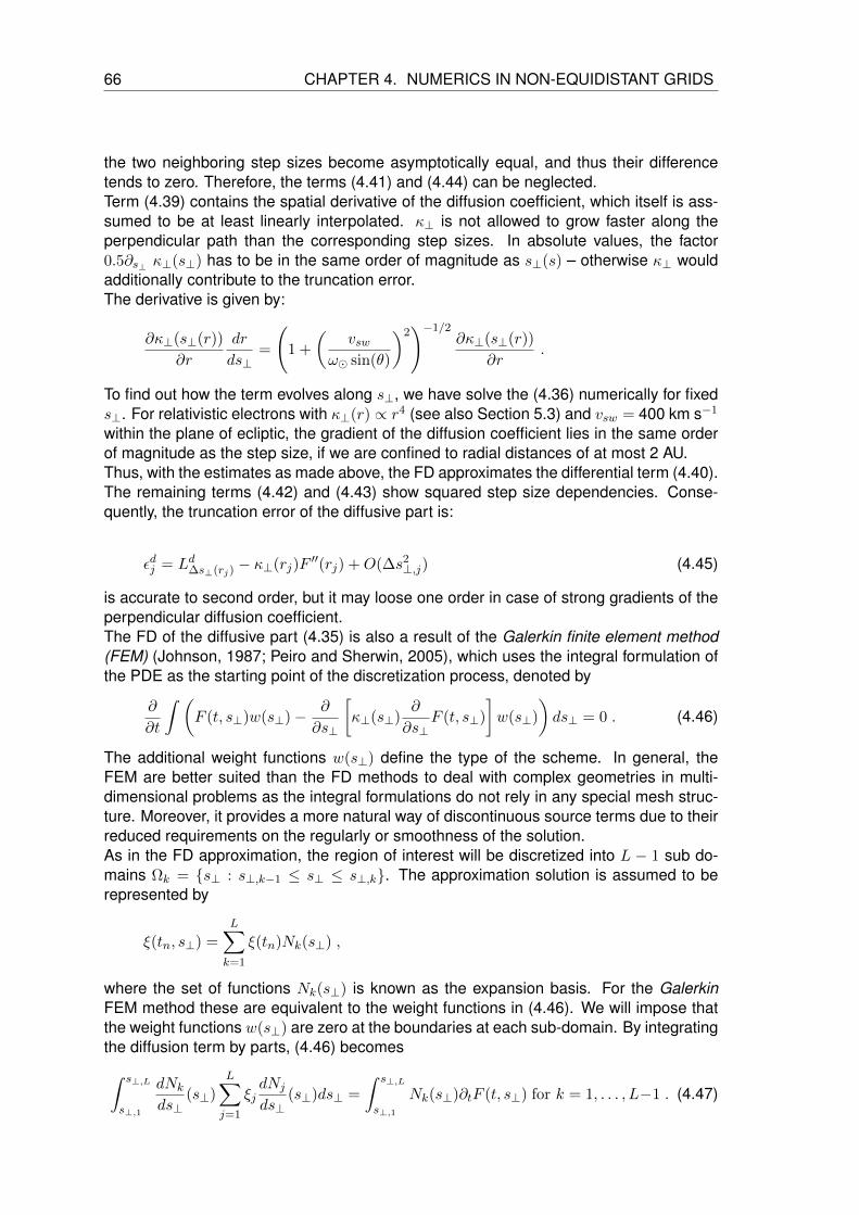
66 CHAPTER 4. NUMERICS IN NON-EQUIDISTANT GRIDS
the two neighboring step sizes become asymptotically equal, and thus their differencetends to zero. Therefore, the terms (4.41) and (4.44) can be neglected.Term (4.39) contains the spatial derivative of the diffusion coefficient, which itself is ass-sumed to be at least linearly interpolated. κ⊥ is not allowed to grow faster along theperpendicular path than the corresponding step sizes. In absolute values, the factor0.5∂s⊥ κ⊥(s⊥) has to be in the same order of magnitude as s⊥(s) – otherwise κ⊥ wouldadditionally contribute to the truncation error.The derivative is given by:
∂κ⊥(s⊥(r))
∂r
dr
ds⊥=
(1 +
(vsw
ω sin(θ)
)2)−1/2
∂κ⊥(s⊥(r))
∂r.
To find out how the term evolves along s⊥, we have solve the (4.36) numerically for fixeds⊥. For relativistic electrons with κ⊥(r) ∝ r4 (see also Section 5.3) and vsw = 400 km s−1
within the plane of ecliptic, the gradient of the diffusion coefficient lies in the same orderof magnitude as the step size, if we are confined to radial distances of at most 2 AU.Thus, with the estimates as made above, the FD approximates the differential term (4.40).The remaining terms (4.42) and (4.43) show squared step size dependencies. Conse-quently, the truncation error of the diffusive part is:
εdj = Ld∆s⊥(rj)− κ⊥(rj)F
′′(rj) +O(∆s2⊥,j) (4.45)
is accurate to second order, but it may loose one order in case of strong gradients of theperpendicular diffusion coefficient.The FD of the diffusive part (4.35) is also a result of the Galerkin finite element method(FEM) (Johnson, 1987; Peiro and Sherwin, 2005), which uses the integral formulation ofthe PDE as the starting point of the discretization process, denoted by
∂
∂t
∫ (F (t, s⊥)w(s⊥)− ∂
∂s⊥
[κ⊥(s⊥)
∂
∂s⊥F (t, s⊥)
]w(s⊥)
)ds⊥ = 0 . (4.46)
The additional weight functions w(s⊥) define the type of the scheme. In general, theFEM are better suited than the FD methods to deal with complex geometries in multi-dimensional problems as the integral formulations do not rely in any special mesh struc-ture. Moreover, it provides a more natural way of discontinuous source terms due to theirreduced requirements on the regularly or smoothness of the solution.As in the FD approximation, the region of interest will be discretized into L − 1 sub do-mains Ωk = s⊥ : s⊥,k−1 ≤ s⊥ ≤ s⊥,k. The approximation solution is assumed to berepresented by
ξ(tn, s⊥) =
L∑k=1
ξ(tn)Nk(s⊥) ,
where the set of functions Nk(s⊥) is known as the expansion basis. For the GalerkinFEM method these are equivalent to the weight functions in (4.46). We will impose thatthe weight functions w(s⊥) are zero at the boundaries at each sub-domain. By integratingthe diffusion term by parts, (4.46) becomes∫ s⊥,L
s⊥,1
dNk
ds⊥(s⊥)
L∑j=1
ξjdNj
ds⊥(s⊥)ds⊥ =
∫ s⊥,L
s⊥,1
Nk(s⊥)∂tF (t, s⊥) for k = 1, . . . , L−1 . (4.47)

4.5. TRANSPORT PERPENDICULAR TO THE IMF 67
This represents a linear system of L− 1 equations with L− 1 unknowns: ξ2, ..., ξL.The basis functions are set to have a compact support, meaning that their value andtheir derivatives are different from zero only on the elements containing the node k , forexample,
Nk(s⊥) =
s⊥−s⊥,k−1
∆s⊥,k−1/2s⊥,k−1 < s⊥ < s⊥,k
s⊥,k+1−s⊥∆s⊥,k+1/2
s⊥,k < s⊥ < s⊥,k+1
.
This means that the only integrals different from zero in (4.47) are∫ s⊥,k
s⊥,k−1
dNk
ds⊥
(ξk−1
dNk−1
ds⊥+ ξk
dNk
ds⊥
)ds⊥ +
∫ s⊥,k+1
s⊥,k
dNk
ds⊥
(ξkdNk
ds⊥+ ξk+1
dNk+1
ds⊥
)ds⊥
=
∫ s⊥,k
s⊥,k−1
Nk∂tF (t, s⊥)ds⊥ +
∫ s⊥,k+1
s⊥,k
Nk∂tF (t, s⊥)ds⊥
The right-hand side can be evaluated using a simple integration rule like the trapezoidalrule: (
∆s⊥,k−1
2+
∆s⊥,k2
)∂tF (t, s⊥) .
Inserting the basis functions and its derivatives and putting ∂tF (t, s⊥) on one side alone,we finally get the FD term for the diffusive part, which is identical to the one derived onthe basis of Taylor series approximation.
The FD scheme in s⊥ is incorporated within the summarized approximation method,where the time derivative is represented by the first-order forward difference scheme.Thus, the overall truncation error is a sum of all single truncation errors (4.34) and (4.45):
ξn+1j − ξnj
∆t= Lc∆s⊥ + Ld∆s⊥ +O(∆t,∆s⊥,j) . (4.48)
4.5.2. Stability
As part of the summarized approximation and time-splitting method (the time derivativehas been replaced by the first-order, one sided FD), we decided to solve the schemeimplicitly. This has already done for the pure diffusive transport (Laasonen scheme).Laasonen (1949) illustrated that the scheme works stable for all choices of step sizesand all magnitudes of κ⊥. Even in case of very small convective flux (compared to thediffusive one), the scheme can be applied without any stability problems.In contrast to the pure diffusive transport, the additional advective term can lead to os-cillations. This is in contraction to the analytical solution where all transport parameters/coefficients are set to be constant. This might lead to physically unreasonable negativephase-space density. If the FDs are chosen as described above, this three-point approx-imation leads to linear equation system as follows:
Ayn+1 = yn (4.49)

68 CHAPTER 4. NUMERICS IN NON-EQUIDISTANT GRIDS
with
yn = (ξnm,1, ξnm,2, ξ
nm,3, . . . , ξ
nm,lz−1, ξ
nm,lz)
T ∀m ∈ [1, ls] (for each perp. curve) .
The entry ξm,2 corresponds to the numerical value of the distribution function F at location(rlz−l+m, ϕl) at time t = tn. The coefficient matrix is in tri-diagonal shape – the main andthe two neighboring diagonals are filled with non-zero values.An inner row of the coefficient matrix A can be written as:
aj+1 =∆tvsw⊥,j+1/2
∆s⊥,j−1 + ∆s⊥,j−
2∆tκ⊥,j+1/2
∆s⊥,j(∆s⊥,j−1 + ∆s⊥,j)
aj = 1 +∆t(vsw⊥,j+1/2 − vsw⊥,j−1/2)
∆s⊥,j−1 + ∆s⊥,j+
2∆t
∆s⊥,j−1 + ∆s⊥,j
(κ⊥,j+1/2
∆s⊥,j+κ⊥,j−1/2
∆s⊥,j−1
)
aj−1 = −∆tvsw⊥,j−1/2
∆s⊥,j−1 + ∆s⊥,j−
2∆tκ⊥,j−1/2
∆s⊥,j(∆s⊥,j−1 + ∆s⊥,j)
Important for stability is that the system matrix A is a non-singular M-matrix (see alsoGrossmann and Roos, 1994). It should be noted that this postulate corresponds to theone for stability under the maximum norm (maximum principle, see Richtmyer and Morton(1967) or Samarskij (2001) on p. 258–264). Numerical schemes of parabolic or hyper-bolic PDEs, that are stable under the maximum norm, are even stable with respect tothe Von-Neumann stability analysis, thus we limit ourselves to investigate the M -matrixproperties.This implies that matrix A = (ai,j) is either weakly column or weakly row-diagonal-dominant:
|ai,i| ≥∑j 6=i|ai,j | ; i, j ∈ [0, 1, . . . , N ] ;row-dominance in row i .
The strict inequality must hold for at least one i.
Moreover, A has to be non-singular :
det A 6= 0, A− = (a−ij) ≥ 0 and aij ≤ 0 ∀i 6= j
and an irreducible L-matrix :
aii > 0 i ∈ N ∀ aij < 0 ∀i 6= j
These conditions assure that A can be inverted in order to get the F -values for the nexttime step.Checking the diagonal dominance with regard to the matrix coefficients aj−1, aj andaj+1, we can directly see that it is always fulfilled with |ai,i| −
∑j 6=i |ai,j | = 1 i, j ∈
[0, 1, . . . , N ].Being an irreducible L-matrix requires that al−1 and al+1 have to be negative. But in thefirst row, we can not keep the condition when convection becomes more pronounced than

4.6. INITIAL AND BOUNDARY CONDITIONS 69
diffusion. If the simulations parameters are chosen that way, we are forced to introduce alimiting factor, which adds additional artificial (numerical) diffusion:
Xj+1/2 = ρj+1/2 coth (ρj+1/2) with ρj+1/2 =vsw⊥,j+1/2∆s⊥,j−1 + ∆s⊥,j
4κ⊥,j+1/2(4.50)
aj+1 =∆tvsw⊥,j+1/2
∆s⊥,j−1 + ∆s⊥,j−
2∆tκ⊥,j+1/2
∆s⊥,j(∆s⊥,j−1 + ∆s⊥,j)Xj+1/2
aj = 1+∆t(vsw⊥,j+1/2 − vsw⊥,j−1/2)
∆s⊥,j−1 + ∆s⊥,j+
2∆t
∆s⊥,j−1 + ∆s⊥,j
(κ⊥,j+1/2Xj+1/2
∆s⊥,j+1/2+κ⊥,j−1/2Xj−1/2
∆s⊥,j−1/2
)
aj−1 = −∆tvsw⊥,j−1/2
∆s⊥,j−1 + ∆s⊥,j−
2∆tκ⊥,j−1/2
∆s⊥,j(∆s⊥,j−1 + ∆s⊥,j)Xj−1/2
In case of vanishing solar-wind convection, we have pure diffusive, stable transport, andX tends to 1. In case of increasing convection X increases and adds some additionaldiffusive flux.
4.6. Initial and boundary conditions
At the beginning of the simulation, and with inclusion of solar wind effects, all numericalvalues of the distribution function have been set to ε = 1E − 10. The p′ transport co-efficients are very small compared to those of the other numerical values. Operationsbetween these and vanishing particle numbers could lead to underflow errors. Conse-quently, we have chosen ε to be much larger than smallest absolute value of floating pointnumbers – which is about 10−23 for single precision (32-bit). Since all particle speciesare distributed uniformly by ε and since the overall mass of injected particles is manyorders of magnitude higher than ε, this additional particle population can be related to theomnipresent background plasma in interplanetary space.The source functionQ in (3.9) is realized as time-varying inner boundary in the s-transport(Section 4.2). As first approximation, the injection is located at the footpoint of the centralfield line (CFL). The CFL itself is positioned in the middle of the grid at ϕ = 0 to avoidboundary effects. Alternatively, an extended source along the perpendicular curve canbe applied as well (n=1, see blue-colored line in Figure 4.4). The source is incorporatedin terms of field-parallel transport (s‖-transport):
ξn+11,l = ξn1,l −
∆t(vµ+ vsw,‖,1/2)
∆s‖,1,lξn1,l +
∆t(vµ+ vsw,‖,3/2)
∆s‖,1,lq(tn, s⊥,l) (4.51)
q(tn, s⊥,l) has been scaled with respect to time and space. Thus, the total number ofinjected particles is kept constant and the temporal evolution is conserved even if the gridresolution and the time step size change.Although we can not assure mass conservation for each energy bin, because of themomentum transport, we would like to prevent particles to get lost by other transport

70 CHAPTER 4. NUMERICS IN NON-EQUIDISTANT GRIDS
processes. In order to have a conservative scheme for perpendicular transport, we intro-duced reflection for the diffusive part. The refraction coefficient ν (see also Lampa, 2006)is set to zero.According to the Neumann boundary condition, we have set the diffusive fluxes to zeroat s⊥,1 and s⊥,lz :
κ⊥(s‖, s⊥)∂F (s‖, s⊥)
∂s⊥
∣∣∣∣s‖=sj ,s⊥=s⊥,1
≈ κ⊥,j,1ξj,1 − ξj,2∆s⊥,j,1
= 0 ,∀j ∈ [1, ls] ,
and
κ⊥(s‖, s⊥)∂F (s‖, s⊥)
∂s⊥
∣∣∣∣s‖=sj ,s⊥=s⊥,lz
≈ κ⊥,j,lz−1ξj,lz−1 − ξl,j
∆s⊥,j,lz= 0 ,∀j ∈ [1, ls] .
Since ξ1, ξ2, ξlz−1 and ξlz are not to supposed to be zero during simulation time, we haveto demand that the coefficients
κ⊥,j,1∆s⊥,j,1
= 0 andκ⊥,j,lz
∆s⊥,j,lz= 0
vanish. Introducing reflection for SEPs would not be adequate because the particlesare swept westward: Particles, that have been reflected at the most western boundary,would immediately be transported to the cell they originally came from. From the mosteastern site, particles would not expected to be produced out of nothing. Thus the fluxat that location will be zero. Numerical reflection would be redundant since there areno particles that could make a reversal in direction. In sum, we have set the convectivefluxes to zero.
F cj,1 = vsw,⊥,j,1ξ1 − ξ2
2= 0 and F cj,lz = vsw,⊥,j,lz
ξj,lz−1 − ξj,lz2
= 0
⇔ vsw,⊥,j,lz = vsw,⊥,j,1
The upper row in the system matrix for perpendicular transport yields (without Il’in cor-rection):
aj,1 = 1−∆tvsw⊥,j−1/2
∆s⊥,j−1 + ∆s⊥,j+
2∆t
∆s⊥,j−1 + ∆s⊥,j
(κ⊥,j−1/2
∆s⊥,j−1
),
aj,2 = −∆tvsw⊥,j−1/2
∆s⊥,j−1 + ∆s⊥,j−
2∆tκ⊥,j−1/2
∆s⊥,j−1(∆s⊥,j−1 + ∆s⊥,j),
and the lower row yields:
aj,lz−1 = −∆tvsw⊥,j−1/2
∆s⊥,j−1 + ∆s⊥,j−(
2∆tκ⊥,j−1/2
∆s⊥,j∆s⊥,j−1
),
aj,lz = 1−∆tvsw⊥,lz+1/2
∆s⊥,j−1 + ∆s⊥,j+
2∆t
∆s⊥,j−1 + ∆s⊥,j
(κ⊥,j−1/2
∆s⊥,j−1
).
Comparing to Section 4.5.2, the stability criterion holds even at the boundaries. It shouldbe noted that the western boundary acts as an boundary reservoir whereas the mosteastern areas get void. The particle accumulation can be overcome either by just simu-lating till the first particles reach the western boundary. Consequently, the model covering

4.6. INITIAL AND BOUNDARY CONDITIONS 71
(a) Partially covered ecliptic plane (b) Fully covered ecliptic plane
Figure 4.4.: Numerical grid of the ecliptic plane, including colored curvatures: Green linesindicate the boundary conditions for perpendicular transport, blue lines theinitial and boundary conditions for field-parallel transport.
partially the ecliptic plane (see left panel in Figure 4.4) would be adequate. If the CFL islong enough – in the sense that it rolls up more than 360 – the original perpendicularcurves can be elongated (e.g. curve number 1 combines with former number 13 in the leftpanel of Figure 4.4). The boundary segment, which is the closed to the Sun, shortens, ifthe footpoint of the CFL is shifted to smaller radial distances. Nevertheless, this segmentis not expected to affect the simulation results significantly since most particles are sweptout due to focusing before a recognizable spread in azimuth occurs, as it is evident in e.g.Figure 6.3.


5. Simulation Assumptions
First of all, all fits are based on a larger number of assumptions: (a) The large scalestructure of the background medium is uniform (constant solar wind, no deviation fromthe Archimedean spiral); neither shocks and magnetic clouds nor corotating interactionregions influence the focusing length. (b) Scattering conditions are also assumed to beconstant (conventionally, the radial particle mean free path λr is assumed to be constantin space and time). (c) In general, differences in scattering conditions between differentflux tubes, as indicated e.g. in the sudden flux-drop outs or the propagation channels(see discussion in Chapter 7.2.3), are not considered. Such differences probably wouldbe encountered by the observer due to the satellite’s relative motion to the backgroundmedium, although at least from turbulence measurements it is not clear whether themedium is more structured as a checker board or in terms of streams (Stevens andKasper, 2007; Zhang, Russell, Baumjohann, Jian, Balikhin, Cao, Wang, Blanco-Cano,Glassmeier, Zambelli, Volwerk, Delva and Voros, 2009).Some exceptions from the constancy of λr in azimuth were made to explain the obser-vations during the crossing of sector boundaries and regions of different propagationproperties (see Section 7.2.2).
5.1. SEP injections and boundary conditions
The injection function Q in (3.9) depends on location, time, pitch-cosine and momentum.The source term is made separable by
Q(s⊥,0, t, µ′, p′) = q1(s⊥,0) · q2(t) · q3(µ′) · q4(p′) . (5.1)
Numerically, Q has been realized as a time-varying inner boundary, which is equivalentto the footpoints of the modeled field lines (see Section 4.6). Concerning its spatial de-pendencies, it is not necessarily a point-like source term, but might be extended eitherdescribed by the Gaussian distribution or a rectangular function (also expressed in termsof two Heaviside step functions). For program user information Section A.3 will give someinsight.The source particles are set to be isotropically distributed in the positive pitch-cosine.Other pitch-angle distribution do not considerably exhibit different results, since the strongfocusing produces high, Sun outward-directed anisotropies.The time evolution is either point-like as a Dirac delta function (also called δ-function) ora Reid-Axford profile (Reid, 1964):
q2(t) ∝ 1
texp
(− tct− t
tL
)(5.2)
with tc being the coronal diffusion time and tL the loss time. It should be noted thatthis is just a convenient and conventional parametrization. Both parameters in principledescribe diffusive propagation from a point source through the corona combined with aloss of particles, but there is no evidence for such a process to occur in the corona.
73

74 CHAPTER 5. SIMULATION ASSUMPTIONS
Based on observational data, we adopted from Ruffolo (1994) the momentum spectrumthat is expected to follow a power law according to
F (p′) = F0
(p′
p′0
)−δ′, (5.3)
with δ′ = 5.
5.2. Assumptions regarding field-parallel transport
Various observations of SEP transport have shown, that particle propagation ranges fromalmost scatter-free (with free mean paths of the order of 1 AU) to strongly diffusive (withλ about 0.01 AU); for most events λ‖ is between 0.08 and 0.3 AU - termed as the Palmerconsensus range (Bieber et al., 1994; Palmer, 1982). Although any scattering parameterderived from observations is model-dependent (Zhang et al., 2007), values of λr lyingwithin the domain [0.01 AU,1.0 AU] have found to be plausible.In this study, the spatial dependence of λ‖ is assumed such that the radial mean freepath λr is constant. Support stems from earlier observations giving power law indicesβ for the radial dependence λr ∼ rβ ranging from 0 to 0.6 (Beeck et al., 1987; Hamil-ton, 1977; Zwickl and Webber, 1977). Without considering an explicit radial dependence,Wibberenz et al. (1992) and Muller-Mellin et al. (1993) argued from fits (using differentone-dimensional propagation models) on particle events observed outside 3 AU for verysimilar local values of λ compared to observations inside 1 AU. These results suggest atmost a slight increase of λr with radius. We will therefore adopt the earlier, successful ap-proach of λr to be constant. As a consequence, the parallel mean free path λ‖ increaseswith increasing radial distance as
λ‖(r) = λr sec2 ψ . (5.4)
The pitch-angle diffusion coefficient (PADC), defined in Section 2.4.2 as
κµ(µ) = A(
(1− sign(µ)σ) |µ|q−1 +H) (
1− µ2), (5.5)
is directly related to the free mean path by (2.55).According to the quasi-linear theory (QLT) and the slab model of magnetic field fluctu-ations, the PADC is restricted to forms of κµ(µ) ∝ |µ|q−1 (1− µ2
). Both left- and right-
handed circularly polarized waves are assumed to be present equally, forming linearlypolarized fluctuations (σ = 0). H is set zero, thus the filling of a possible gap aroundµ = 0 is neglected.In Figure 5.1, some shapes of the PADC are shown. A comparison between these the-oretical predictions and the observed solar particle data, performed by Beeck and Wib-berenz (1986), showed that the pitch-angle diffusion coefficient “has a minimum near 90
pitch angle” which is even more pronounced than in earlier studies by Bieber et al. (1980)where they predicted q = 1.2 and H = 0.We chose q = 1.6 and H = 0 to realize damped scattering for low µ-values and comparedthe resulting numerical solution of (3.1) with the one using isotropic pitch-angle scattering
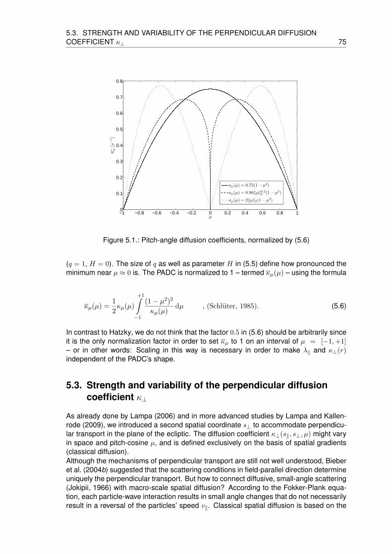
5.3. STRENGTH AND VARIABILITY OF THE PERPENDICULAR DIFFUSIONCOEFFICIENT κ⊥ 75
−1 −0.8 −0.6 −0.4 −0.2 0 0.2 0.4 0.6 0.8 10
0.1
0.2
0.3
0.4
0.5
0.6
0.7
0.8
µ
κµ[s
−1]
κµ(µ) = 0.75(1 − µ2)
κµ(µ) = 0.96‖µ‖0.22 (1− µ2)
κµ(µ) = 2‖µ‖2(1− µ2)
Figure 5.1.: Pitch-angle diffusion coefficients, normalized by (5.6)
(q = 1, H = 0). The size of q as well as parameter H in (5.5) define how pronounced theminimum near µ ≈ 0 is. The PADC is normalized to 1 – termed κµ(µ) – using the formula
κµ(µ) =1
2κµ(µ)
+1∫−1
(1− µ2)2
κµ(µ)dµ , (Schluter, 1985). (5.6)
In contrast to Hatzky, we do not think that the factor 0.5 in (5.6) should be arbitrarily sinceit is the only normalization factor in order to set κµ to 1 on an interval of µ = [−1,+1]– or in other words: Scaling in this way is necessary in order to make λ‖ and κ⊥(r)independent of the PADC’s shape.
5.3. Strength and variability of the perpendicular diffusioncoefficient κ⊥
As already done by Lampa (2006) and in more advanced studies by Lampa and Kallen-rode (2009), we introduced a second spatial coordinate s⊥ to accommodate perpendicu-lar transport in the plane of the ecliptic. The diffusion coefficient κ⊥(s‖, s⊥, µ) might varyin space and pitch-cosine µ, and is defined exclusively on the basis of spatial gradients(classical diffusion).Although the mechanisms of perpendicular transport are still not well understood, Bieberet al. (2004b) suggested that the scattering conditions in field-parallel direction determineuniquely the perpendicular transport. But how to connect diffusive, small-angle scattering(Jokipii, 1966) with macro-scale spatial diffusion? According to the Fokker-Plank equa-tion, each particle-wave interaction results in small angle changes that do not necessarilyresult in a reversal of the particles’ speed v‖. Classical spatial diffusion is based on the

76 CHAPTER 5. SIMULATION ASSUMPTIONS
Brownian motion, where a single particle-particle collision changes the particle’s propa-gation direction considerably. The link between these macro-scale quantities – which isimmanent in the mean free path λ‖ – and small-scale turbulence in µ has already beendone in (2.55).κ⊥ is suggested to depend on radial distance only, thus we limit ourselves to the radial co-ordinate r instead of (s‖, s⊥). Note that different (s‖, s⊥) could describe the same r. Sinceperpendicular diffusion occurs in one dimension alone, the parallel diffusion coefficientκ‖ and λ‖ are related as:
κ‖(r) =1
2vλ‖(r) . (5.7)
To make κ⊥(r, µ) dependent on κ‖(r), the factor γ has been introduced:
κ⊥(r, µ) = γ κ‖(r) . (5.8)
As suggested by Palmer (1982), we assume λ⊥/λ‖ to be constant with λ⊥/λ‖ ≈ 1/10 asthe upper boundary at r = 1 AU. As an conservative estimate of the influence of perpen-dicular transport, values of λ⊥/λ‖ close to unity as suggested by Dwyer et al. (1997) andZhang et al. (2003) are not considered. Since the numerical integration of particle trajec-tories in realistic 3D interplanetary magnetic field turbulence gives λ⊥/λ‖ ≈ 0.02−0.04 forthe cross-field transport (Giacalone and Jokipii, 1999) – comparable to the ratio derivedfrom the analysis of 2D turbulence Matthaeus et al. (2003) – we chose λ⊥/λ‖ ≈ 1/50as the lower boundary. The ratios are fixed at 1 AU and, according to the Friedmann-Lemaitre-Robertson-Walker metric scaled as r2.Another confirmation for the squared radius dependence of κ⊥ comes from Zhang, Qinand Rassoul (2009), who stated that perpendicular diffusion is “inversely proportional tolocal magnetic field strength”. This is physically reasonable since perpendicular scatter-ing is assumed to be very strong in isotropic distributions – which is the case at largerdistances from the Sun.Moreover, the theory of the graphical random walk of field lines suggests that perpen-dicular displacements are supposed to be of the order of magnitude of the gyro-radiusrL = mv⊥/(|q|B0(r)). Since B0(r) ∝ r−2 for r < 1, this would lead to the r2 dependency,too. Unfortunately, FLRW is based on field line displacements instead of spatial shifts ofthe particle’s gyro-centers relatively to field line which is magnetically connected to theinjection site. The field line meandering, as suggested by the FLRW, could not explain thefast azimuthal propagation and wide spread of SEPs in studies of Kallenrode (1993a).In contrast to this work, Jokipii showed that the ratio between the perpendicular and theparallel diffusion coefficient derived from the Fokker-Planck equation is proportional tothe inverse square to the mean magnetic field, yielding an even higher power in radialdistance: κ⊥ : κ‖ ∝ r4 sec2 Ψ.Nevertheless, several studies, based on observations and/or theory, supported thesquared radius dependency of the λ⊥-to-λ‖-ratio.Consequently, the perpendicular diffusion coefficient yields:
κ⊥(r) = γ3 v2r2
16
∫ +1
−1
(1− µ2)2
κµ(r, µ)dµ , with γ ∈ [0.02, 0.1] . (5.9)
So far, we did not discuss the pitch-angle dependence of perpendicular transport. In caseof pitch-angle independent transport of high energetic particles, as it has been realizedin early studies in the ecliptic plane, the model resembles the Parker’s Equation (Parker,

5.3. STRENGTH AND VARIABILITY OF THE PERPENDICULAR DIFFUSIONCOEFFICIENT κ⊥ 77
1965). Note that both models are similar but not equal since the Parker equation is basedon spatial diffusion. Moreover, we also consider focusing in diverging magnetic fields fromRoelof which significantly affects energetic particles very close to the Sun.The µ-independence has two consequences: i) the particle’s pitch angle is conservedduring cross-field transport and ii) the likelihood of cross-field transport does not dependon pitch-angle.Numerical simulations by Zhang, Qin and Rassoul (2009) have shown that even a µ-dependent κ⊥ would produce similar results: Perpendicular diffusion due to micro-scaleturbulence becomes noticeable when particles have undergone “enough” pitch-anglescattering. This is the case when particles have already left the very inner heliosphere.In these regions (depending on λr), distributions are nearly isotropic and diffusion actssimilarly on particles with different pitch-angles.Although Zhang, Qin and Rassoul assumed that perpendicular scattering is very strongin isotropic distributions, we introduced some simple µ dependencies and made a com-parison with isotropic scenarios (Section 5.3.1).Numerically, κµ(s‖, s⊥, µ) is incorporated via a splitting of the pitch-angle diffusion coeffi-cient into a spatial-dependent and a pitch-cosine-dependent part:
κµ(s‖, s⊥, µ) = κµ(s‖, s⊥) · κµ(µ), (5.10)
with κµ(s‖, s⊥) = κr cos2(Ψ(s‖, s⊥)) and the normalized pitch-angle diffusion coefficientκµ(µ) as defined in the previous Section 5.2.
5.3.1. Does cross-field transport depend on rigidity?
In Section 5.3, some assumptions about the variability and dependencies of κ⊥ weremade on the basis of several studies. The still missing part is the validation of the depen-dencies in terms of the current model.Whereas the total amount of perpendicular transport is determined as an average of thePADC over all pitch-angles µ = [−1,+1] (5.9), we thought about an explicit µ-dependenceof κ⊥ as it has already been introduced in field-parallel direction.For first estimates, we choose κ⊥ to be the following µ-dependent functions:
κ⊥(µ) = 3µ2 and κ⊥(µ) =3
2
(1− µ2
)Both κ⊥s have been scaled in such that
κ⊥(µ) = κ⊥(µ)/
(∫ +1
−1κµ(µ)dµ
),
thus the total mount of diffusive flux is equal – whatever the shape of κ⊥(µ) looks like.The overall diffusion coefficient in perpendicular direction yields κ⊥(r, µ) = κ⊥(r)κ⊥(µ)(separation approach). The total strength is incorporated implicitly in the radial term, asit is seee in (5.9).At least the (1− µ2)-dependency has a plausible physical meaning. If κ⊥ is defined as in(5.9), combined with the assumption of λr to be constant, κ⊥ yields:
κ⊥(r, µ) = κ⊥(r) κ⊥(µ) ∝ v2(1− µ2)r2
(cos (Ψ))2. (5.11)

78 CHAPTER 5. SIMULATION ASSUMPTIONS
κ⊥(r, µ) can be interpreted in terms of rigidity P (2.6) as
κ⊥(r, µ) ∝ P 2
(cos (Ψ))2, (5.12)
where the spiral term solely originates from the assumption of a constant radial meanfree path λr.Several theories – among them the quasi-linear-theory (QLT) – suggested the parallelmean free path λ‖ to grow with increasing rigidity P (see Section 2.1.1). Instead of acontinuous loss of particles from the observer’s site in field-parallel direction, these lossescould also be explained by enhanced cross-field transport, as it has been introduced hereby (5.12).
0 2 4 6 8 1010
2
104
106
108
1010
time [h]
inte
nsity
[arb
. uni
ts]
κ⊥(µ) = 1
κ⊥(µ) = 32(1− µ2)
κ⊥(µ) = 3µ2
r = 0.3 AU, ϕ= 0 CFLr = 1.0 AU, ϕ= 0 CFLr = 0.3 AU, ϕ= 30 westr = 1.0 AU, ϕ = 30 west
(a) Intensity-time profiles
0 2 4 6 8 10
0
0.5
1
1.5
2
2.5
time [h]
anis
otro
py
κ⊥(µ) = 1
κ⊥(µ) = 32(1− µ2)
κ⊥(µ) = 3µ2
r = 0.3 AU, ϕ= 0 CFLr = 1.0 AU, ϕ= 0 CFLr = 0.3 AU, ϕ= 30 westr = 1.0 AU, ϕ = 30 west
(b) Anisotropy-time profiles
Figure 5.2.: Intensity-time profiles at different locations. The standard scenario was cho-sen, but κ⊥ : κ‖ is set to 1/50. Three possible shapes for the µ-dependentpart of the perpendicular diffusion coefficient were assumed: κ⊥(µ) = 1(isotropic scattering, solid lines), κ⊥(µ) = 3
2(1 − µ2) (dashed lines) andκ⊥(µ) = 3µ2 (dot-dashed lines).
Some of the results can be seen in Figure 5.2. For illustration, 10 MeV protons withspeed vp = 1 AU h−1 were chosen because they are expected to be more sensitive tointerplanetary scattering than relativistic electrons. Again, the impulsive and punctualinjection takes place at the footpoint of the central field line (CFL) with particles beingisotropically distributed in positive pitch-angle.At first glance, one can state that the introduction of µ-dependent perpendicular trans-port does not affect the SEPs that much as adiabatic cooling does (see Section 6.4 forcomparison). Deceleration as a consequence of the expanding solar wind leads to fasterdecay rates once the bulk of particles has passed the observer. Here, on the other hand,changes in omni-directional intensity and first-order anisotropy can be only observed inthe very early phase of particle detection.Within r = 0.3 AU at the CFL, no significant deviations can be observed. Since κ⊥(r)is suppressed by the scaling with r2, the cross-field loss of particles is marginal. Atazimuthal distance ϕ = 30, the intensity is 4 orders of magnitude smaller than at theCFL. In case of κ⊥ ∝ 1−µ2 the diffusive flux is marginally higher than in case of isotropicdiffusion, since the dominant particle population with µ ≈ 1 is favored. The other term

5.4. THE STANDARD SCENARIO 79
κ⊥(µ) ∝ µ2 with the opposite effect in µ behaves neutral because there are no particleshaving a significant velocity component in field-perpendicular direction.These changes can be better identified when looking at the anisotropies: For κ⊥(µ) ∝ µ2,they are higher beyond the CFL than in terms of isotropic scattering, but they also decayfaster.The SEPs behave in the same manner (compared to r = 0.3 AU) at the radial distancer = 1 AU, even if the temporal evolution occurs on different scales.The crucial feature, that causes these differences, is the pitch-angle distribution. Early inthe event, the particles are highly isotropic – not just because of the injection profile butalso by the pitch-angle focusing which keeps particles to be field-aligned within the firsttenths of an AU. As they propagate outward, they subsequently undergo pitch-angle scat-tering which leads to isotropic distributions. This is the reason why the curves becomeidentical 1 - 3 hours after the first SEPs have reached the observer.But not only the “youth” of an event is important, but also the phase when the first particlesarrive at the observer. This is why even at r = 1 AU, the profiles differ. Consideringjust a single energy band with no additional adiabatic deceleration, the first particleswould be the ones that have a mostly field-aligned velocity component, and consequentlythey contribute to the highest anisotropies in the particle distribution. Note that evenadditional adiabatic cooling would not affect the results considerably since this wouldlead to changes in the decay phase (phase when the maximum of particles has alreadyleft the observer, see Section 6.4 for comparison).Without the r2 scaling, the curves would have the tendency to differ more within r = 0.3 AU.With the inclusion of the scaling and the nearly isotropic distributions beyond r = 0.3 AU,the effects of pitch-angle dependent cross-field transport are negligible at all observationpoints. The effects become more pronounced if the ratio of κ⊥ : κ‖ increases, but arenegligibly small compared to those of solar wind effects (see Section 6.4).
5.4. The standard scenario
To simplify the description of the various simulation runs in the two following Chapters 6and 7, we define a set of parameters and assumptions that uniquely identifies a scenario- termed standard scenario.
variable value descriptionv 1 AU h−1 particle’s speed
λr 0.1 AU mean free path in radial direction, related to 10 MeV protons with v= 1 AU h−1
γ 0.1 ratio perpendicular–to–parallel diffusion coefficient at 1 AUsini 0.1 AU injection position and footpoint of the CFL
vsw0.0096 AUh−1 solar wind speed (corresponds to vsw = 400 km s−1)
θ 1.5708 rad helio-latitude (corresponds to θ = 90; ecliptic plane θ ≈ 83)q1(s‖,0), q2(t =0)
δ(sini) source term
Table 5.1.: Standard scenario defining the default set of parameters. All quantities can bereviewed in the appendix A.1.


6. Validation and Tests
Validation of the numerics as a whole is impossible since it consists of a compositionof separated and consecutively executed transport processes. The resulting data mightbe reasonable but we can not exclude that one single transport process still has somenumerical inconsistencies or errors. Nevertheless, there are some general features thatmust be fulfilled during the entire simulation time.First, particles are not allowed to be swept out of the system – except for the fact that weexplicitly allow particles to leave the system, for example at the spatial boundaries in field-parallel as well as in perpendicular direction, or, as it realized for momentum transport,towards lower momenta.Secondly, detection of negative particle populations would give evidence to erroneousFortran code or to a violated stability criterion. Abrupt changes in intensities, oscillationsin intensities or non-smooth surface plots within the ecliptic plane would also fit into thiscategory.Third, according to the model construction, particles are expected to be transported in asingle bulk with a single center of mass which should be located in an area between theCFL and the radially outward directed tangent at the footpoint of the CFL.A complete validation includes both a separate test of each transport process (see Sec-tion 6.1 and 6.2) and a comparison to already existing schemes. At least within the veryinner heliosphere, where the IMF lines are almost radial, a comparison with the resultsof the azimuthal model introduced by Lampa and Kallenrode (2009) should give similartime- and azimuthal profiles (Section 6.3).
6.1. Field-parallel Transport
As it is illustrated in Section 4.2, the explicit Lax-Wendroff scheme works stable in themaximum norm even if step sizes along the field lines are not equidistant anymore. Un-fortunately, the accuracy of the finite differences (FD) drops to one.The corresponding code was tested by switching off all other schemes in µ, p and s⊥. Atdifferent times, intensity- and anisotropy plots or data files were made in order to comparethem with those of uniform step sizes. The solar wind speed was switched off to makethe overall particles speed in the solar rest frame constant (see Figure 6.1).Phase space density neither reaches negative values nor any oscillations as an indica-tor of violated stability conditions were observed. The total mass of particles remainsconstant, except for a very vanishing (0.1 %) fraction that gets lost due to rounding er-rors at transport coefficients γ(sj , µi) and η(sj , µi). These values are partially dividedby very small step sizes ∆sj . The s-transport works exact for the fastest particles withvmax = µmaxv. The truncation error εj,i vanishes, and at least these particles will beshifted exactly to the next following grid point.As it is described in Section 5.1, particles are injected isotropically in the positive pitch-angle domain. Combined with a δ-injection in time, this results in 20 different field-parallelparticle velocities, Figure 6.1 features 20 peaks in case of constant step sizes. With
81

82 CHAPTER 6. VALIDATION AND TESTS
0 5 10 1510
4
105
106
107
108
109
time [h]
inte
nsity
[arb
. uni
ts]
∆s = 1E-3 AU∆s = 1E-2 AU∆s(r,∆ϕ = 20) [AU]∆s(r,∆ϕ = 5) [AU]∆s(r,∆ϕ = 5)∗ [AU]
(a) Omnidirectional intensity
0 5 10 150
0.5
1
1.5
2
2.5
3
time [h]
anis
otro
py
∆s = 1E-3 AU∆s = 1E-2 AU∆s(r,∆ϕ = 20) [AU]∆s(r,∆ϕ = 5) [AU]∆s(r,∆ϕ = 5)∗ [AU]
(b) Anisotropy
Figure 6.1.: Profiles along the magnetic field line for 10 MeV protons (v = 1 AU h−1) attime t = 10.1 hours: Only field-aligned advection is considered, solar windand pitch-cosine transport is ignored, δ injection at sini = 0.1 AU.
increasing step sizes, the green curve shows a pronounced broadening compared to theblue curve at a higher resolution. This results from a numerical dissipation and dispersionerror in the first-order upwind-scheme (“numerical diffusion”, see Hatzky (1996), page53). Even the anti-diffusive fluxes of the flux-limiter method can not prevent the gradientsto be smeared out with time. In the current model, ∆s(s) grows and exceeds an orderof magnitude with increasing s – compared to the innermost step size at the field line’sfootpoint. This is why the peaks disappear beyond s = 1 AU.Some particles are transported faster out than it would be physically reasonable (beyonda radial distance of 10.2 AU). The original, numerical model stops advancing in spacebeyond that barrier (note that this is not the outer boundary), otherwise a fraction ofSEPs would propagate faster than they actually are. This behavior can be also seenin the current model (see violet curves), but by default, the scheme considers all gridpoints because – in combination with enhanced perpendicular transport – especially themost eastern field lines could be filled with additional particle populations ahead of thepropagation front.If pitch-cosine transport is added besides advection along the IMF line, all profiles be-come very similar. The curves seem to be congruent for almost the entire path – exceptfor the regions where the first particles arrive (see discussion above) and for the foot-points. The reason is that actually the injection is not peak-like in space but extended by∆s(sini) (with sini being the CFL footpoint’s location). The source term as a time-varyinginner boundary acts like an extended source in case of a coarse-meshed grid. Note that∆s(sj) itself depends both on s and ∆ϕ.The conclusion in terms of one-dimensional, field-aligned transport is that even with vary-ing step sizes, the results are well in agreement with those of constant ∆s. Because ofthe first-order accuracy, the results of the introduced scheme depend strongly on the gridresolution. It is recommended to work with adequately small ∆s (∆ϕ) with ∆ϕ = 5 andbelow – not because of the approximation error in the FDs but because of the focusinglength (3.7) whose discrete values are overestimated for too large step sizes (for detailssee Section 6.5).

6.2. FIELD PERPENDICULAR TRANSPORT 83
Outer boundary
We have two choices to overcome those effects emerging from the outer boundary atrout. As in the conventional model we are able to allow particle to fully or partially leavethe region under investigation. This can be done by making a change in the reflection co-efficient which is 1 for full reflection and zero for complete passage into the outer space.We are mainly interested in particle behavior in the very inner heliosphere, which is upto the Earth’s orbit (up to 1 AU). Particles that are backscattered significantly due to theouter boundary, could distort the results.The outer boundary will be fixed beyond 5 AU radial distance, which is sufficient even forthe fastest particles not to reach it during simulation time (for most computed scenarios).Larger values are not physically reasonable, because at these distances beyond the Jo-vian orbit, the assumption of Archimedean spirals certainly is no longer valid valid andcorotating interaction regions will have formed.This results from the growing step sizes in field-parallel and in perpendicular direction. Achange in rout does not involve a significant additional amount of grid points. Moreover– as we have seen in the Numerics chapter – time step sizes are chosen according tothe stability criteria at the footpoints of the field lines. This is at rini = 0.1 AU as default,where the footpoints form the inner boundary. The minimum value lies at about 0.06 AU.Consequently, an extension of the ecliptic grid does not lead to a massive increase incomputing time or in memory allocation.
6.2. Field perpendicular transport
Assuming that the perpendicular diffusion coefficient κ⊥ is constant (isotropic scatter-ing) and that the source is impulsive, point-like injection of m0 particles at location z0 (in[AU])(δ-injection), an enclosed, analytical solution of the diffusion equation
∂f
∂t=
∂
∂z
(κ⊥(s, z)
∂f
∂z
)(6.1)
is possible. The area under consideration has to be infinite to both sides. It should benoted that – at least in this Section – f will be treated in units of linear density, since thetransport is only governed by simple spatial diffusion in one dimension.Then, both a Laplace-transform according to the time t and a Fourier transform accordingto the space can be applied (for details see Farlow, 2003).Remember that the Fourier transform can be defined as
F [f(z)] =1√2π
∫ +∞
−∞exp (iωz)f(z)dz = F (ω) , (6.2)
under the assumption that the improper integral is bounded. Note that in literature, thereis no unique definition for the Fourier transform. Definitions might differ in different scal-ings to the preceding factor and to ω.If the first n derivatives of f(z) exist, the following formula would help to apply the trans-form to Equation 6.1:
F [f (k)(z)] = (iω)kF [f(z)] k = 1, . . . , n (6.3)

84 CHAPTER 6. VALIDATION AND TESTS
The Laplace transform can be applied to continuous functions of exponential order c, ifthere exists a M > 0 and c > 0 in the sense that the inequality
|f(t)| ≤M exp (c t)
is fulfilled for all t ∈ [0, ∞ [ .According to the stability in the maximum norm, f(t, z) is bounded between 0 andm0/dz(r)(dz(r) is the width of the cell where the particles are injected) – given by the minimal val-ues of the boundary conditions and the maximum value of the initial condition. Since allupper-bounded functions are automatically functions of exponential order zero, f(z) canbe Laplace-transformed without any constraints.
Definition of the Laplace transform for functions of exponential order c:
L[f(t)] =
∫ +∞
0exp (st)f(t)dt = L(s) . (6.4)
The integral is absolutely convergent, if s > c (in this case: s > 0).
Theorem:If the first n derivatives of f(z) exist and these are all of exponential order c, the Laplacetransform of the kth derivative of f(t) gives for s > c:
L[f (k)(t)] = skL[f(t)]− sk−1f(0)− sk−2f ′(0)− · · · − f (k)(0) k = 1, . . . , n . (6.5)
The tools will help to get an enclosed solution to the heat conduction (6.1). Using thetransformation τ(t) = κ⊥t, (6.1) can be rewritten:
∂u
∂τ=∂2u
∂z2∈ Ω = [(z, τ)| −∞ < z < +∞, 0 ≤ t <∞] (6.6)
with u(z, τ = 0) = Γ(z) being the initial condition. Concerning this diffusion problem, wehave Γ(x) = m0δ(z), the Dirac-δ-function:
δ(z) =
m0δ(0) for z = 0
0 for z 6= 0;
∫ +∞
−∞δ(z)dz = m0 ;
∫ +∞
−∞f(z) δ(z)/m0dz = f(0) .
The solution of (6.1) will be given by the solution of (6.6) by f(z, t) = u(z, κ⊥t).
First, the PDE (6.6) will be Laplace-transformed with respect to τ . The transformed valueof u(x, τ) is defined as U(x, s). Using (6.5), we get:
∂xxU(x, s)− sU(x, s) = Γ(z) with Γ(z) = u(z, τ = 0) .
Now, the PDE will be Fourier-transformed with respect to the spatial variable z. Thetransformed function of U(s, τ) is called V (ω, s). Let Φ(ω) be the transformed function ofΓ(z).According to Equation (6.3), the upper equation yields:
−ω2V (ω, s)− sV (ω, s) = Φ(ω)⇔ V (ω, s) =Φ(ω)
ω2 + s; .
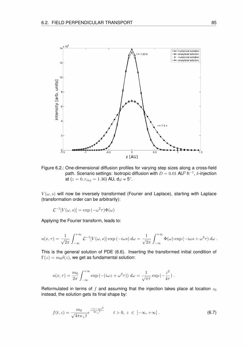
6.2. FIELD PERPENDICULAR TRANSPORT 85
Figure 6.2.: One-dimensional diffusion profiles for varying step sizes along a cross-fieldpath. Scenario settings: Isotropic diffusion with D = 0.01 AU2 h−1, δ-injectionat (z = 0, rinj = 1.36) AU, dϕ = 5.
V (ω, s) will now be inversely transformed (Fourier and Laplace), starting with Laplace(transformation order can be arbitrarily):
L−1[V (ω, s)] = exp (−ω2τ)Φ(ω)
Applying the Fourier transform, leads to:
u(x, τ) =1√2π
∫ +∞
−∞L−1[V (ω, s)]·exp (−iωs) dω =
1√2π
∫ +∞
−∞Φ(ω)·exp (−iωs+ ω2τ) dω .
This is the general solution of PDE (6.6). Inserting the transformed initial condition ofΓ(z) = m0δ(z), we get as fundamental solution:
u(x, τ) =m0
2π
∫ +∞
−∞exp (−(iωz + ω2τ)) dω =
1√πτ
exp (− z2
4τ) .
Reformulated in terms of f and assuming that the injection takes place at location z0
instead, the solution gets its final shape by:
f(t, z) =m0√4πκ⊥t
e−(z−z0)
2
4κ⊥t t > 0, z ∈ [−∞,+∞] . (6.7)

86 CHAPTER 6. VALIDATION AND TESTS
Comparing the numerical solutions with (6.7) implies that, during simulation time, noparticles reach the outer boundaries. An adequate distance zd between the injectionlocation and the outer boundary can be defined, where just the fraction ε of the totalmass m0 has reached the boundaries after the time tc (Lampa, 2006):
zd = z0 +√−ln
(ε√
4πκ⊥t)
4κ⊥tc ε ∈ [0, 1]. (6.8)
The computed diffusion profiles are expected to be similar to the analytical solution forε→ 0.As numerical scheme, the implicit Laasonen scheme was chosen, since the diffusioncoefficient is expected to be highly variable in the inner heliosphere. An explicit schemelike the Crank-Nicolson-scheme (Crank and Nicolson, 1947) would require the stabilitycriterion
κ⊥(r)∆t
∆z(r)2≤ 1 .
A κ⊥(r) scaled with the squared radius would grow faster than ∆z(r)2, thus the criterionwill be violated beyond a certain radial distance. Moreover, the Laasonen scheme worksproperly even at strong gradients (e.g. at possible shock fronts, and in the early phase ofan event at the injection location. As a consequence, the truncation error in t drops to theorder of one.Figure 6.2 illustrates two different kind of diffusion profiles, the first taken at t ≈ 2 hours,and the other at t ≈ 8 hours. The step sizes along the perpendicular curve grow inpositive (westward) direction. They were computed according to an azimuthal resolutionof ϕ = 5. The δ-injection occurred at rinj = 1.36 AU and released a total mass of particleof m0 = 1E + 11/∆z(rinj) . The diffusion coefficient was set to κ⊥ = 0.01 AU2 h−1.Numerical solutions are indicated by crosses + while the exact solutions are denoted bydiagonal crosses x. Each pair of profiles coincide perfectly except for the area around theinjection location where the numerical f lies slightly under the exact solution. The reasonis that the particles are injected numerically as an extended source with width ∆z(rinj).This is why these differences are pronounced in the early phase. Despite the fact thatthe step sizes vary with radial distance, we still get symmetrical profiles. No oscillations,that would cause negative linear densities, were observed. Thus the scheme is stable– even with other sets of parameters, that could violate the stability criterion for explicitschemes. Moreover, the total particles number m0 =
∑lzl=1 f(zl)∆zl stays constant. For
t → ∞, the z interval was uniformly filled with particles without any losses. Thus, eventhe total reflection at the outer boundaries works as it was expected.
Periodic boundary conditions were tested by plotting f along the complete perpendicularpath. By the introduction of periodicity, segments of perpendicular paths, that were orig-inally separated from each other, were sticked together (see Figure 4.4). The resultingprofiles were smooth along the complete interval. Abrupt changes would have been anindicator that the array indexing failed.Alternatively, the entire plane of ecliptic was checked with respect to smooth surfaces ofintensity and anisotropy (see e.g. Figure 6.3 in the following Section 6.3).

6.3. AZIMUTHAL VS. PERPENDICULAR CROSS-FIELD TRANSPORT 87
6.3. Azimuthal vs. perpendicular cross-field transport
Time-profiles and spatial distributions are expected to be similar within 0.3 AU, since bothgrids are very similar and look like a radial magnetic field in that region. So, this Sectionis dedicated to a test of the complete model – but ignoring the solar wind effects.We took the standard scenario which is defined as in Section 5.4 and chose ∆s = 0.001AU for the azimuthal model in order to have spatial resolutions of the same magnitude.But even a value for ∆s, which is ten times larger, will not change the numerical resultssignificantly – as we have already validated in Section 6.1. A first glance at a snapshot
(a) Perpendicular transport (b) Azimuthal transport
Figure 6.3.: Intensity-plots in the ecliptic plane at time t = 5 h in two different numeri-cal grids. The simulation parameters have been chosen with respect to thestandard scenario.
of the ecliptic plane (Figure 6.3) indicates that cross-field diffusion acts much strongeron particles in the perpendicular grid than in the azimuthal one, even though the diffu-sion coefficients themselves are the same. This underestimation in the former grid hasalready been mentioned by Lampa and Kallenrode (2009). Azimuthal displacements donot effectively separate particles from the CFL beyond 1 AU, since ∠(eϕ, es) (cf. Figure3.3) decreases with increasing radial distance.
At r = 0.3 AU, spatial distributions are almost identical. This can be seen even betterwhen looking at the azimuthal profiles at the left panel of Figure 6.4. With increasingtime, all profiles get levelled off: Particles are swept towards the flanks and tend to bedistributed equally in space.Both profiles (azimuthal and perpendicular) have in common that particles are displacedto both sides of the CFL in the same amount: The graphs are symmetric around the CFL,which is in good agreement with the assumption that the field has to be nearly radialwithin r = 0.3 AU.Significant differences arise when we look at r = 1.0 AU: The azimuthal profiles seem toindicate that particles are not distributed as far as in the perpendicular ones (as seen inthe 2D-profiles). Moreover, particles are obviously swept into western direction. The bulkcenter (maximum of particles) is located slightly to west, whereas the azimuthal profiles

88 CHAPTER 6. VALIDATION AND TESTS
−90 −60 −30 0 30 60 9010
4
105
106
107
108
109
CFL westeast
ϕ[]
inte
nsity
[arb
. uni
ts]
t = 1 ht = 5 ht = 10 h
perpendicular transportazimuthal transport
(a) r = 0.3 AU
−90 −60 −30 0 30 60 9010
4
105
106
107
108
109
CFL westeast
ϕ[]
inte
nsity
[arb
. uni
ts]
t = 1 ht = 5 ht = 10 h
perpendicular transportazimuthal transport
(b) r = 1.0 AU
Figure 6.4.: Azimuthal variation of the omni-directional intensity
still show symmetric graphs. The reason is that particles at radial distance beyond 1 AUundergo a slight displacement in positive radial direction when they are swept westward.In eastward direction, the SEPs are slightly shifted towards the Sun. Thus, in situ mea-surements at a constant radial distance, the onset of the very first arriving particles aswell as the maximum of particles is expected to be detected earlier on the western flankthan on the opposite side if the CFL. This is clearly visible in the intensity-time-profiles(Figure 6.5).The anisotropy-time profiles in both realizations of cross-field transport qualitatively showalways the same behaviour, which is typically observed in impulsive SEP events: Anabrupt rise very early in the event and gradual decrease towards zero in the followinghours. But both grid architectures have in common, that the more we look azimuthallybeyond the CFL the more the anisotropy falls and even changes to negative values. Thisdecrease is even more pronounced in the western direction of the perpendicular grid.This can be explained by the fact that perpendicular diffusion coefficient κ⊥ is scaled withthe squared radius:Hours after the simulation start and within a few tenth of 1 AU, some of the neighboringfield lines might not yet be filled with particles considerably, whereas the rest of the fieldline already shows significant particle populations. These particles are subsequentlybackscattered and reduce the net flux of particles streaming away from the Sun. If theamount of inward flux exceeds the outward flux, this results in negative anisotropies.Note that this happens beyond ϕ ± 60 and weak cross-field diffusion. At larger radialdistances, this negative anisotropy is not observed in the model.
6.4. Introduction of solar wind effects
Figure 6.6 demonstrates the time development of SEPs, when solar wind effects areinvolved. Remember that in contrast to Ruffolo’s approach, the reference frame is therest frame of the solar magnetic field, with µ and p measured in solar wind frame. Theobserver is located at a fixed field line, but the solar wind’s orientation was not transformedby the additional corotation speed. Instead, solar wind particles flow radially outward with
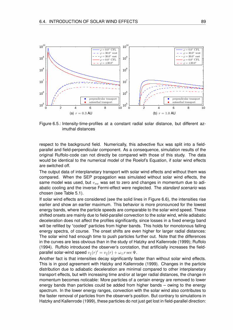
6.4. INTRODUCTION OF SOLAR WIND EFFECTS 89
0 2 4 6 8 1010
5
106
107
108
109
1010
ϕ= 0.0 CFLϕ= 30.0 westϕ= 30.0 eastϕ= 0.0 CFLϕ= ±30.0
perpendicular transportazimuthal transport
(a) r = 0.3 AU0 2 4 6 8 10
105
106
107
108
109
1010
ϕ= 0.0 CFLϕ= 30.0 westϕ= 30.0 eastϕ= 0.0 CFLϕ= ±30.0
perpendicular transportazimuthal transport
(b) r = 1.0 AU
Figure 6.5.: Intensity-time-profiles at a constant radial solar distance, but different az-imuthal distances
respect to the background field. Numerically, this advective flux was split into a field-parallel and field-perpendicular component. As a consequence, simulation results of theoriginal Ruffolo-code can not directly be compared with those of this study. The datawould be identical to the numerical model of the Roelof’s Equation, if solar wind effectsare switched off.The output data of interplanetary transport with solar wind effects and without them wascompared. When the SEP propagation was simulated without solar wind effects, thesame model was used, but vsw was set to zero and changes in momentum due to adi-abatic cooling and the inverse Fermi-effect were neglected. The standard scenario waschosen (see Table 5.1).If solar wind effects are considered (see the solid lines in Figure 6.6), the intensities riseearlier and show an earlier maximum. This behavior is more pronounced for the lowestenergy bands, where the particle speeds are comparable to the solar wind speed. Theseshifted onsets are mainly due to field-parallel convection to the solar wind, while adiabaticdeceleration does not affect the profiles significantly, since losses in a fixed energy bandwill be refilled by “cooled” particles from higher bands. This holds for monotonous fallingenergy spectra, of course. The onset shifts are even higher for larger radial distances:The solar wind had enough time to push particles further out. Note that the differencesin the curves are less obvious than in the study of Hatzky and Kallenrode (1999); Ruffolo(1994). Ruffolo introduced the observer’s corotation, that artificially increases the field-parallel solar-wind speed v‖(r)′ = v‖(r) + ωr sec Ψ.Another fact is that intensities decay significantly faster than without solar wind effects.This is in good agreement with Hatzky and Kallenrode (1999). Changes in the particledistribution due to adiabatic deceleration are minimal compared to other interplanetarytransport effects, but with increasing time and/or at larger radial distances, the change inmomentum becomes noticable: More particles of a certain energy are removed to lowerenergy bands than particles could be added from higher bands – owing to the energyspectrum. In the lower energy ranges, convection with the solar wind also contributes tothe faster removal of particles from the observer’s position. But contrary to simulations inHatzky and Kallenrode (1999), these particles do not just get lost in field-parallel direction:

90 CHAPTER 6. VALIDATION AND TESTS
0 2 4 6 8 10
100
102
104
106
108
time [h]
inte
nsity
[arb
. uni
ts]
11 MeV protons, vp = 1 AU h−1
125 MeV protons, vp = 3.4 AU h−1
1060 MeV protons, vp = 6.4 AU h−1
including solar wind effects
without solar wind effects
(a) r = 0.3 AU
0 2 4 6 8 10
100
102
104
106
108
time [h]
inte
nsity
[arb
. uni
ts]
11 MeV protons, vp = 1 AU h−1
125 MeV protons, vp = 3.4 AU h−1
1060 MeV protons, vp = 6.4 AU h−1
including solar wind effects
without solar wind effects
(b) r = 1.0 AU
Figure 6.6.: Intensity-time profiles including (solid lines) and without (dashed lines) solarwind effects for different energies. The default parameter set was chosenaccording to the standard-scenario.
They were shifted to neighboring field lines in western direction. The central field line willnot be adequately refilled from the opposite direction since the injection occurred at theCFL and the bulk of particles does not show the tendency to broaden of even shift itscenter to the east.The same features can be observed in the first-order anisotropies (not shown here). Atlate times, they can even become negative since the main part of the particle distributionwas convected across the observer. This leads to an inward directed intensity gradientand finally to a streaming of particles towards the Sun. The negative values are lesspronounced than in earlier studies by Hatzky and Kallenrode (1999). The reason couldbe that the neighboring field lines still contribute enough particles streaming outward.
6.5. Spatial resolution of the grid and its impact on thenumerical results
Before making any fits to the satellite observations, the crucial question has to be an-swered if and how the simulation results differ with different spatial resolutions. Notethat this also incorporates a change in time step size, since the minimum step size infield-parallel direction is coupled with ∆t via the stability criterion (4.21).Again, the default parameter set according to the standard scenario is chosen, but ne-glecting the effects of the solar wind. As a first step, the focus was taken to pure field-parallel transport, including the particle’s gyro center motion along the magnetic field line,focusing due to the diverging magnetic field and pitch-angle scattering. Four scenariosare compared with each other (see Figure 6.7), two of them are based on the originalfinite difference scheme for constant step sizes (∆s = 0.001 AU, indicated by blue lines;and ∆s = 0.01 AU, indicated by the green lines). Scenarios 3 and 4 already incorpo-rate variable step sizes along s, that have been computed with respect to an azimuthalresolution of ∆ϕ = 1 (red lines) and ∆ϕ = 5 (cyan lines) (see Section 3.2.2, (3.28)).It is obvious that the time-profiles do not coincide for an observer at r = 0.3 AU as well as

6.5. SPATIAL RESOLUTION 91
0 1 2 3 4 510
6
107
108
109
1010
time [h]
inte
nsity
[arb
. uni
ts]
∆s = 1E-3 AU∆s = 1E-2 AU∆s(r,∆ϕ = 1) [AU]∆s(r,∆ϕ = 5) [AU]
r = 0.3 AUr = 1.0 AU
(a) Intensity-time profiles
0 1 2 3 4 50
0.5
1
1.5
2
2.5
3
time [h]
anis
otro
py
∆s = 1E-3 AU∆s = 1E-2 AU∆s(r,∆ϕ = 1) [AU]∆s(r,∆ϕ = 5) [AU]
r = 0.3 AUr = 1.0 AU
(b) Anisotropy-time profiles
Figure 6.7.: Time profiles for pure field-parallel transport at different locations: Differentgrid resolutions were chosen: Constant step sizes ∆s = 0.001 AU (blue lines)and ∆s = 0.01 AU (green lines) as well as variable step sizes correspondingto ∆ϕ = 1 (red lines) and 5 (cyan lines). The default parameter set waschosen according to the standard-scenario, but ignoring solar wind effects.Particles are 10 MeV protons with speed v = 1 AU h−1.
1 AU. With increasing step size, as indicated in Figure 6.7, the test particles arrive laterat the observer: the delays between the injection and the first arriving particles (illus-trated best by a sudden rise in the anisotropies) is more pronounced at larger distances.Note that this is independent of the step size choice (constant or variable step sizes).Moreover, these delays can not be explained in terms of inaccuracies of the finite differ-ences, in particular the observer’s location: The delay between the two times of maximumanisotropy in non-equispaced grids (red and cyan curves) yields ≈ 0.25 hours – corre-sponding to a 0.25 AU distance between the maximum anisotropies. This is at least onemagnitude higher than the step sizes at r = 1 AU (∆s⊥(r = 1AU,∆ϕ = 5) ≈ 0.01 AU;∆s⊥(r = 1AU,∆ϕ = 1) ≈ 0.06 AU).The discrete solutions of the finite difference schemes do not considerably differ, butthese differences are evident especially in the early phase of the event and along thepropagation front. Larger step sizes can be best identified in the very fine structures of thetime profiles, such as the anisotropy peaks. Note that vanishing particle numbers werecut off to defend anisotropies from statistical errors. What makes the difference in theexample mentioned above, and in general, is the focusing length, which is expected to behighly variable within 0.3 AU. Due to numerical construction reasons combined with a fastdecrease of the inverse focusing length (see Figure A.5), the pitch-angle-focusing termwithin the µ-scheme is overestimated for large spatial step sizes: Field-parallel transportand focusing are executed consecutively, but not at the same time: Once a particle wasfocused according to the local magnetic field structure, it will be shifted to next followinggrid point on the field line. If the jump becomes too large, this might also lead to aconsiderable change in the magnetic field, which was not taken into account when thefocusing was applied in the previous time step. Note that these numerical effects emergeboth in grids with constant and varying step sizes. For future studies (in case of constantstep sizes along the field lines), it would be more adequate to determine the focusing

92 CHAPTER 6. VALIDATION AND TESTS
0 1 2 3 4 510
4
106
108
1010
time [h]
inte
nsity
[arb
. uni
ts]
r = 0.3 AU,ϕ = 0
r = 1.0 AU,ϕ = 0
r = 0.3 AU,ϕ = 30 westr = 1.0 AU,ϕ = 30 west
∆ϕ = 1
∆ϕ = 5
(a) Intensity-time profiles
0 1 2 3 4 5
0
0.5
1
1.5
2
2.5
3
time [h]
anis
otro
py
r = 0.3 AU,ϕ = 0
r = 1.0 AU,ϕ = 0
r = 0.3 AU,ϕ = 30 westr = 1.0 AU,ϕ = 30 west
∆ϕ = 1
∆ϕ = 5
(b) Anisotropy-time profiles
Figure 6.8.: Time profiles for different grid resolutions: 1 (blue lines) and 5 (red lines)at different locations. The default parameter set was chosen according tothe standard-scenario, but ignoring solar wind effects. Particles are 10 MeVprotons with speed v = 1 AU h−1.
length on the basis of average magnetic conditions between two neighboring grid pointson a field line instead of a single point. The numerical grid of the current model is sufficientto represent the highly variable focusing length close to the Sun.Pitch-angle focusing has strong influence on the simulation results, since it is the onlytransport process that dominates within a few tens of an AU. The other effects in inter-planetary transport would lead to different results in the decay phase late in the event.Here, the results differ in very early phase (with five hours after the injection occurs),while the profiles become similar once this period has expired. It should be emphasizedthat these similar profiles are not a result of strong diffusion that levels out any gradients(see e.g. Figure 6.4). These studies showed that the profiles become similar for differentspatial resolutions, but on different levels – depending on the observer’s location.
With additional cross-field diffusion and for small step sizes ∆ϕ, the azimuthal profiles atfixed times reveal a stronger confinement of particles around the CFL (7.5 less withinthe first 5 hours for the current scenario). The difference lies in the same order of mag-nitude as the larger angular resolution of ∆ϕ = 5. Therefore, it can be discussed interms of inaccuracies of the numerical scheme. As long as the test particles are locatedwithin 0.3 AU, no significant spread in azimuth occurs - because of the r2 scaling of theperpendicular diffusion coefficient, and because of the finer grid meshes.The dominating contribution of pitch-angle focusing over scattering in µ become lesssignificant, thus particles have the tendency to become isotropic earlier than in caseof larger spatial step sizes. Therefore, particles need more time to escape to largerradial distances (see Figure 6.8). This has already been shown for the one-dimensionaltransport, but additional cross-field transport leads to even slightly higher time differences.For ∆ϕ = 5 and r = 1 AU, the first particles arrive about 15 minutes earlier than in the1D case: Especially beyond r = 0.3 AU, particles experience additional Sun outwarddirected displacements, when they are transported westward across the field lines, andwhen they are subsequently backscattered onto the CFL. It should be noted that just

6.5. SPATIAL RESOLUTION 93
a small fraction of the injected particles (approximately 0.1% of the maximum intensity)contributes to these differences.In order to have reasonable onset times, it is recommended not to choose crude angularresolutions larger than ∆ϕ = 5, since this would lead to significant differences from thehighly resolved (≤ 1) solutions - as a result of both numerical focusing and cross-field-transport effects.


7. Model Results
Using the numerical model based on the Ruffolo’s equation and the additional perpendic-ular diffusion, this section will be dedicated to the dynamics of cross-field transport. Thepropagation parameters, that have been introduced in one-dimensional transport, will beadopted as well as the estimate for the perpendicular diffusion coefficient (see Section5.3). Parameter studies in Section 7.1 will illustrate the dynamics of the introduced 2-dimensional transport in the ecliptic plane. The resulting intensity- and anisotropy-timeprofiles will be validated with respect to the azimuthal spread of type III radio bursts (Sec-tion 7.2.1) as well as the multi spacecraft observations (Section 7.2.3).
7.1. A parameter study
The intent of this section is to estimate the possible influence of perpendicular transport,but not to fit energetic particle events. Scenarios with different parameter sets will beapplied in order to illustrate how the particle spread evolves in space and time – depend-ing on the parameter configuration. The results are checked with respect to plausibilityand we will look for a physical explanation. A first impression about the dynamics of thetwo-dimensional transport without solar wind effects were already gained in Section 6.3using the standard scenario.The parameter sets are also based on the standard scenario (5.1), but the focus is takenon particle velocities of v = 1, 3.4 and 6.4 AU h−1. The radial mean free path is set to theupper und lower boundary, which we have been declared to be plausible (Section 5.2).The ratio perpendicular to parallel diffusion strength is set to 1/10 and 1/50 at r=1 AU,and scaled with r2. In sum, six scenarios have been computed.
7.1.1. Plots in the ecliptic plane
Combined effects of field-parallel and field-perpendicular transport can be illustrated bestby looking at the ecliptic plane. The SEPs were injected as a δ-injection onto the field lineoriginating at ϕ = 0. The local parallel particle mean free path is determined from λr =0.1 AU, the perpendicular mfp consequently is 0.01 AU at 1 AU, but scaled with r2.On a logarithmic scale, Figure 7.1 shows the intensity for 10 MeV protons (v = 1 AU h−1)at different times (t = 1 hour in the first row, t = 5 hours in the second and t = 10 h inthe last row). On the left, strong perpendicular diffusion was assumed, on the right theratio was set to one fiftieth. It is evident that with increasing ratio, the spread of particlesin azimuth is more pronounced – note just because of the scaling with γ = 1/10 or 1/50.Beyond the Earth’s orbit, the squared-radius-dependency of κ⊥ leads to a faster removalof SEPs from the CFL, whereas perpendicular diffusion close to the Sun is suppressed.The field lines shown in the figure are 30 apart. For this example, the area between thedashed field lines (around the CFL) is filled within an hour in case of strong perpendiculardiffusion. Weak cross-field transport accordingly shows lower extents. Thus, enhancedperpendicular diffusion effectively removes more particles from the CFL. The gradients
95
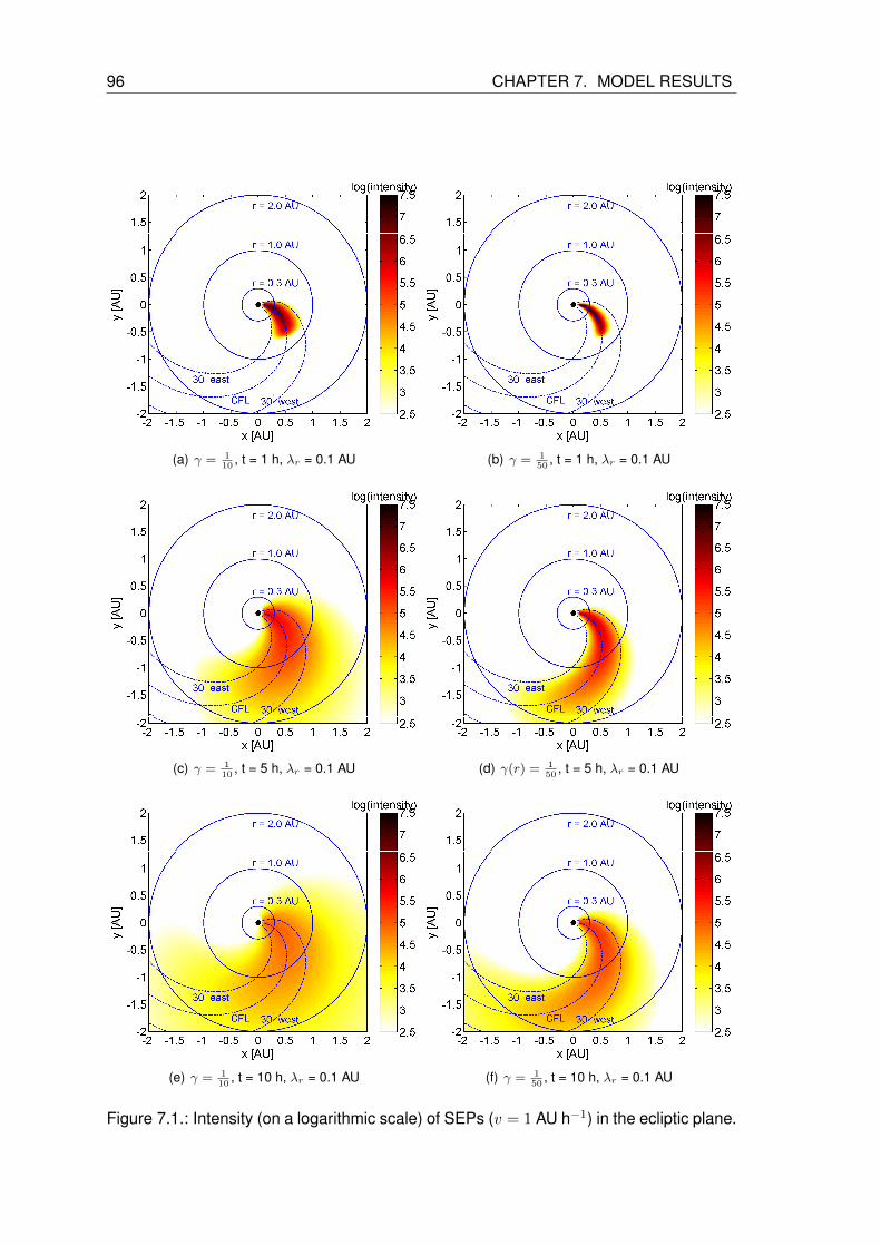
96 CHAPTER 7. MODEL RESULTS
(a) γ = 110
, t = 1 h, λr = 0.1 AU (b) γ = 150
, t = 1 h, λr = 0.1 AU
(c) γ = 110
, t = 5 h, λr = 0.1 AU (d) γ(r) = 150
, t = 5 h, λr = 0.1 AU
(e) γ = 110
, t = 10 h, λr = 0.1 AU (f) γ = 150
, t = 10 h, λr = 0.1 AU
Figure 7.1.: Intensity (on a logarithmic scale) of SEPs (v = 1 AU h−1) in the ecliptic plane.

7.1. A PARAMETER STUDY 97
(a) γ = 110
, λr = 0.01 AU (b) γ = 150
, λr = 0.01 AU
(c) γ = 110
, λr = 0.1 AU (d) γ = 150
, λr = 0.1 AU
(e) γ = 110
, λr = 1 AU (f) γ = 150
, λr = 1 AU
Figure 7.2.: Intensity-plots in the ecliptic plane at time t = 5 h for different scatteringconditions.

98 CHAPTER 7. MODEL RESULTS
in perpendicular direction are leveled off, and the front of the first arriving particles couldnot propagate as far as in the case of strong diffusion.Moreover, the bulk center of particles shifts slightly westward as a consequence of theradially outward streaming solar wind. This can be seen more clearly in the cross-fieldprofiles (see following Section 7.1.2).So far, the model results are as expected, but what about different combinations of theratio κ⊥-to-κ‖ (denoted by γ) and the radial mean free path λr? As an example, Figure7.2 illustrates the spread of particles with v = 1 AU h−1. The snapshots were taken fivehours after the injection, λr varies with 0.01, 0.1 and 1 AU and the diffusion ratio is γ =1/50, 1/10. From top to bottom, λr increases by one order of magnitude in each row; theleft panels were plotted with stronger perpendicular diffusion than the right ones. Themiddle row therefore corresponds to the middle row of Figure 7.1.Discussing about the “horizontal dependencies” (strong vs. weak perpendicular diffu-sion), the same behavior can be observed as in 2D plots that illustrated the temporalevolution of particle transport for both γ = 1/50 and 1/10. The new feature in this contextis that the radial mean free path λr contributes to the overall strength of perpendiculartransport. First, λr determines the strength of pitch-angle scattering along the field lines:Inserting the spatially dependent pitch-angle diffusion coefficient (PADC) (5.10) into (5.9)yields κµ(r) = 0.75 v λ−1
r cos (Ψ)2, which denotes the strength (“amplitude”) of the PADC.The smaller λr is, the more efficiently particles undergo pitch-angle scattering: Distri-butions that have originally been highly anisotropic due to the escape along open fieldlines and due to focusing effects, become consecutively more isotropic. This preventsparticles from leaving the very inner heliosphere (r < 0.3 AU), where the radially scaledperpendicular diffusion coefficient is not able to considerably shift particles in azimuthaldirection. As can be seen in Panel (b) of Figure 7.2) for example, 10 MeV protons with v= 1 AU h−1 are still mainly confined to one AU although 5 hours since the injection havepassed. Secondly, λr acts directly as a scaling factor in κ⊥, since λr is assumed to beconstant: κ⊥ ∝ λ‖ = λr sec (Ψ)2.The opposite case λr = 1 AU, allows SEPs to propagate without significant pitch-anglescattering, so the fastest particles nearly reach 5 AU arc length along the CFL. Unfortu-nately, the SEPs are exposed to strong (radially scaled) cross-field diffusion much earlierthan the ones described in the previous scenario.Consequently, at fixed times, different combinations of κ⊥ : κ‖ and λr lead to differentshapes of the particle distributions. In the latter case (γ = 1
50 , λr = 1 AU), the bulkcenter has been significantly shifted outward. The propagation front rather looks like asemi-circle, covering almost half of the ecliptic plane. The shape resembles a shockfront. Normally, shocks are made responsible for this huge azimuthal spread of particles(180 within a few hours). Low-λr-distributions rather look like a tongue: they are moreextended in field-parallel direction than perpendicular to it. Moreover, there appears tobe no considerable peak of particles. The spatial gradients in field-parallel direction looksmoother than in case of weak pitch-angle scattering: low λr-values and a cross-fielddiffusion coefficient, suppressed by the r2 scaling, lead to a storage of particles within r= 1 AU and ϕ± 30, that could last up to ten hours after the injection.
7.1.2. Cross-field profiles
The azimuthal spread of particles can be better resolved by slices through the two-dimensional distributions for fixed times t = 1, 5 and 10 hours after the injection. Figure7.3 shows the intensity on a logarithmic scale with the central field line being located

7.1. A PARAMETER STUDY 99
−50 0 5010
3
104
105
106
107
ϕ[]
inte
nsity
[arb
. uni
ts]
CFL westeast
t = 1 ht = 5 ht = 10 h
r = 0.3 AUr = 1.0 AU
(a) γ = 110
, v = 1 AU h−1
−50 0 5010
3
104
105
106
107
ϕ[]
inte
nsity
[arb
. uni
ts]
CFL westeast
t = 1 ht = 5 ht = 10 h
r = 0.3 AUr = 1.0 AU
(b) γ = 150
, v = 1 AU h−1
−50 0 5010
0
101
102
103
104
ϕ[]
inte
nsity
[arb
. uni
ts]
CFL westeast
t = 1 ht = 5 ht = 10 h
r = 0.3 AUr = 1.0 AU
(c) γ = 110
, v = 3.4 AU h−1
−50 0 5010
0
101
102
103
104
ϕ[]
inte
nsity
[arb
. uni
ts]
CFL westeast
t = 1 ht = 5 ht = 10 h
r = 0.3 AUr = 1.0 AU
(d) γ = 150
, v = 3.4 AU h−1
Figure 7.3.: Azimuthal profiles of omni-directional intensity for different times (t = 1, 5and 10 hours) und medium pitch-angle scattering conditions (λr = 0.1 AU).The left-handed panels reveal stronger perpendicular diffusion than the righthanded ones. For the first panel row, particle’s speed is fixed at v = 1 AU h−1,for the second at v = 3.4 AU h−1.

100 CHAPTER 7. MODEL RESULTS
at azimuthal distance ϕ = 0. Note that these snapshots were taken for fixed radialdistances r = 0.3 and r = 1 AU, thus these profiles do not correspond to those of acertain perpendicular path. They become even more asymmetric beyond 0.3 AU thanalong a field-perpendicular path (see also Section 6.3). Again, the westward shift canbe observed at r = 1 AU, since the solar wind convection occurs oblique to the field-linedirection. Figure 7.3 confirms that the particle distribution moves slowly westward withincreasing time. Moreover, these displacements do not depend on particle properties –which is not surprising since advection is solely influenced by the surrounding medium(solar wind plasma).Perpendicular diffusion leads to a wider spread for fast particles than for slow particles,since κ⊥ is scaled with squared particle speed v (5.9). Thus, in contrast to the former,azimuthal model by Lampa and Kallenrode (2009), profiles of other particle species cannot be obtained by a simple scaling with v.Concerning the model results, we never observed a complete filling within r = 0.3 –independent of the diffusion parameter set. Pitch-angle focusing as well as the dampedperpendicular diffusion prevents particles to be transported to the opposite site of theSun.Compared to the numerical results of the azimuthal model by Lampa and Kallenrode(2009), significant particle spread up to ±30 around CFL occurs at 0.3 AU within an hourfor λ⊥/λ‖ ≈ 1/10. Within five hours significant particle spread over more than ±60 isobserved even at 1 AU. The spread is slightly higher (10− 15) since, due to geometricalreasons, the perpendicular transport in the former model is underestimated.Nevertheless, particles still quickly fill a wide cone around CFL. For κ⊥/κ‖ = 1/50 theparticles are more closely confined to CFL, leading to higher intensities at ϕ = 0 and aslower azimuthal spread: significant filling of a cone of ±40 around CFL now requiresfive hours rather than one hour for 1 AU h−1 particles. All time scales are longer for slowerand shorter for faster particles.In particular at late times and strong perpendicular diffusion, combined with a large meanfree path λr, the spatial gradients have the tendency to vanish.The anisotropy-azimuth profiles show a decay towards the flanks, that can even reachnegative values. We will discuss this feature in the following section.
7.1.3. Intensity-time and anisotropy-time profiles
The cross-field spread of particles leads to a continuous loss of particles from central fieldline. Consequently, during a SEP event the intensity decays faster than in Roelof’s originalmodel without perpendicular transport and also faster than in the former, azimuthal modelby Lampa and Kallenrode (2009).Figure 7.4 illustrates how the profiles of exact perpendicular transport and one-dimensio-nal transport differ for otherwise identical parameter sets. Perpendicular transport alsoreveals a coherent peak at the CFL, but the intensity is lower and decays faster than inthe case of one-dimensional transport. Moreover, the anisotropy is slightly higher. Thus,in order to cover the one-dimensional profile, a smaller mean free path λr and possibly amore gradual injection-time profile (with a long-lasting decay phase) would be required.The 2D model might help to overcome the magnitude problem of the quasi-linear theory(Bieber et al., 1994), where the mean free paths derived from theory always showed thetendency to be smaller than the fitted ones.Early in the event, the anisotropy-time profiles occasionally show negative values for atime period of 30 minutes up to several hours once the bulk of particles has passed the

7.1. A PARAMETER STUDY 101
0 2 4 6 8 10
104
106
108
time [h]
inte
nsity
[arb
. uni
ts]
1D transportϕ= 0.0 CFLϕ= 30.0 westϕ= 30.0 eastϕ= 60.0 westϕ= 60.0 east
(a) Intensity-time profiles
0 2 4 6 8 10−0.5
0
0.5
1
1.5
2
2.5
time [h]
anis
otro
py
1D transportϕ= 0.0 CFLϕ= 30.0 westϕ= 30.0 eastϕ= 60.0 westϕ= 60.0 east
(b) Anisotropy-time profiles
Figure 7.4.: Intensity- and anisotropy-time profiles at r = 0.3 AU, but different azimuthaldistances. The default parameter (5.1) set without solar wind effects waschosen. The solid black curve denotes one-dimensional transport.
observer: This holds for field lines, that are separated by ±60 from the CFL (see panel(b) in Figure 7.4 or Figure 7.6) and beyond. All parameter combinations, that would leadto more cross-field further out than close to the Sun, could explain the numerical results.As it can be seen in the ecliptic plots (Section 7.1.1), the results can be reproduced forlow particle speeds v, low ratios of κ⊥/κ‖ and high λr. Note that this effect should notbe overestimated, since just small particle population contributes to the inward flux. Theinward flux will probably vanish in the omnipresent background plasma in interplanetaryspace. It should be remarked, that another trigger for negative anisotropies are verystrong, perpendicular displacements: The particles are gradually transported behind theSun and and back to the CFL. As a consequence, a second maximum in intensity occurs.The only scenario revealing these features within r = 1 AU, was for a mean free pathof λr = 6.3 AU and κ⊥ : κ‖ = 0.1 for ∼0.5 MeV electrons (see Figure A.11). Negativeanisotropies can be seen for all field lines there. However, this scenario is rather unlikelyand unreasonable because so far neither multi-spacecraft observations as e.g. (Palmer,1982) nor theoretical results have given any indication for the mean free path to be λr >>1 AU.Besides negatives anisotropies there are also some azimuthal asymmetry that will bediscussed below.Figure 7.5 shows the omni-directional intensity-time profiles for an observer at radial dis-tances of 0.3 AU on CFL and for azimuthal distances of 30 and 60 (panels “a” and “c”)as well as for r = 1 AU and the corresponding azimuthal distances (panels “b” and “d”).The ratio κ⊥–κ‖ was set to γ = 1/10 (panels “a” and “c”) and 1/50 (panels “b” and “d”).Medium pitch-angle scattering conditions (λr = 0.1 AU) were assumed.On the CFL, and compared to the solution without perpendicular transport, both weakand strong perpendicular transport almost reveal identical profiles with a coherent peak,but at a lower maximum intensity and with faster decaying intensities. This is the casefor those particles, that have not yet undergone considerable pitch-angle scattering ontheir way to the observer – thus “spiking” profiles can be observed for < 100 MeV protons(v ≈ 3 AU h−1) up to 0.3 AU and for proton energies above 100 MeV up to 1 AU . These

102 CHAPTER 7. MODEL RESULTS
0 2 4 6 8 1010
2
104
106
108
time [h]
inte
nsity
[arb
. uni
ts]
ϕ= 0.0 CFLϕ= 60.0 westϕ= 30.0 westϕ= 30.0 eastϕ= 60.0 east
(a) γ = 110
, v = 1 AU h−1, r = 0.3 AU
0 2 4 6 8 1010
2
104
106
108
time [h]
inte
nsity
[arb
. uni
ts]
ϕ= 0.0 CFLϕ= 60.0 westϕ= 30.0 westϕ= 30.0 eastϕ= 60.0 east
(b) γ = 150
, v = 1 AU h−1, r = 1 AU
0 2 4 6 8 1010
1
102
103
104
105
106
time [h]
inte
nsity
[arb
. uni
ts]
ϕ= 0.0 CFLϕ= 60.0 westϕ= 30.0 westϕ= 30.0 eastϕ= 60.0 east
(c) γ = 110
, v = 3.4 AU h−1, r = 0.3 AU
0 2 4 6 8 1010
1
102
103
104
105
106
time [h]
inte
nsity
[arb
. uni
ts]
ϕ= 0.0 CFLϕ= 60.0 westϕ= 30.0 westϕ= 30.0 eastϕ= 60.0 east
(d) γ = 150
, v = 3.4 AU h−1, r = 1 AU
Figure 7.5.: Intensity-time profiles at r = 0.3, 1 AU and azimuthal distances ϕ =0,±30,±60. For the first panel row, particle’s speed is fixed at v = 1 AUh−1, for the second at v = 3.4 AU h−1. Medium pitch-angle scattering condi-tions (λr = 0.1 AU) were assumed.

7.1. A PARAMETER STUDY 103
0 2 4 6 8 10−1
−0.5
0
0.5
1
1.5
2
2.5
time [h]
anis
otro
py
ϕ= 0.0 CFLϕ= 60.0 westϕ= 30.0 westϕ= 30.0 eastϕ= 60.0 east
(a) γ = 110
, v = 1 AU h−1
0 2 4 6 8 10−1
−0.5
0
0.5
1
1.5
2
2.5
time [h]
anis
otro
py
ϕ= 0.0 CFLϕ= 60.0 westϕ= 30.0 westϕ= 30.0 eastϕ= 60.0 east
(b) γ = 150
, v = 1 AU h−1
Figure 7.6.: Anisotropy-time profiles at r = 0.3 (left panel) and 1 AU (right panel) andazimuthal distances ϕ = 0,±30,±60. Parameters: v = 1 AU h−1, λr = 0.1AU, corresponding to intensity-time profiles in the top row of Figure 7.5.
spatial thresholds correlate with varying λr.At r = 0.3 AU, the plotted profiles beyond the CFL do not exhibit the coherent peak, insteadprofiles become more rounded. This is also true for larger radial distances, even on theCFL. Thus these profiles would not be described in terms of weak scattering but rather interms of diffusive propagation. These differences compared to the CFL profile increasewith increasing κ⊥/κ‖ as well as with increasing azimuthal and radial distance.Again, the asymmetry in azimuth can be observed by comparing those profiles, wherethe observers are located symmetrically around the injection site (cf. panels (a) and (b) inFigure 7.5). The onset and the intensity maximum on the western flank occur earlier in theevent, especially when the observer is located at r = 1 AU. The temporal differences areeven more evident in the anisotropy profiles. The delays stem from cross-field transportthat provides radial displacements in particular beyond 0.3 AU. Despite these differences,all profiles at a fixed radial distance become continuously similar or even identical: Cross-field diffusion levels off all spatial gradients.Figure 7.7 shows the intensity profiles on logarithmic scale for an observer at a radialdistance of 0.3 AU (left panel) and 1.0 AU (right panel) with varying azimuthal distancesof 0 (CFL), ±30 and ±60 for γ = 0.1. Compared to a scenario with a identical setof parameters, but γ = 0.02 (see Figure 7.8), one can state that in the presence ofdamped perpendicular diffusion, more particles are concentrated close to the CFL, thusin particular the profiles at ϕ ± 60 show lower intensities. The time delays betweenthe start of an impulsive flare and the time when the first arriving particles are detected,is considerably larger than in case of strong cross-field diffusion. The same holds forthe maximum intensities. Qualitatively similar properties of cross-field transport are alsofound for low-energy particles, such as 10 MeV protons with speeds of about vp = 1 AUh−1 (see e.g. again panels (a) and (b) in Figure 7.5). Obviously, the SEPs need additionaltime to perform diffusive cross-field transport.If we fix the ratio of both diffusion coefficients at γ = 0.1 and decrease λr by the factor ten(λr = 0.01, strong pitch angle-scattering, see Figure 7.9), the decay phases last longerand the overall profiles become more rounded – compared to Figure 7.7. The latter

104 CHAPTER 7. MODEL RESULTS
0 2 4 6 8 10−2
−1
0
1
2
3
log(
inte
nsity
[arb
. uni
ts])
ϕ = 0.0 CFLϕ = 60.0 westϕ = 30.0 westϕ = 30.0 eastϕ = 60.0 east
(a) Observer located at r = 0.3 AU
0 2 4 6 8 10−2
−1
0
1
2
3
log(
inte
nsity
[arb
. uni
ts])
ϕ = 0.0 CFLϕ = 60.0 westϕ = 30.0 westϕ = 30.0 eastϕ = 60.0 east
(b) Observer located at r = 1.0 AU
Figure 7.7.: Intensity-time profiles of 0.5 MeV electrons for different azimuthal distancesfrom the CFL. The standard scenario with γ = 0.1 was chosen.
0 2 4 6 8 10−2
−1
0
1
2
3
log(
inte
nsity
[arb
. uni
ts])
ϕ = 0.0 CFLϕ = 60.0 westϕ = 30.0 westϕ = 30.0 eastϕ = 60.0 east
(a) Observer located at r = 0.3 AU
0 2 4 6 8 10−2
−1
0
1
2
3
log(
inte
nsity
[arb
. uni
ts])
ϕ = 0.0 CFLϕ = 60.0 westϕ = 30.0 westϕ = 30.0 eastϕ = 60.0 east
(b) Observer located at r = 1.0 AU
Figure 7.8.: Intensity-time profiles of 0.5 MeV electrons for different azimuthal distancesfrom the CFL. The standard scenario was chosen – except for the followingparameter: γ = 0.02.

7.1. A PARAMETER STUDY 105
0 2 4 6 8 10−2
−1
0
1
2
3
log(
inte
nsity
[arb
. uni
ts])
ϕ = 0.0 CFLϕ = 60.0 westϕ = 30.0 westϕ = 30.0 eastϕ = 60.0 east
(a) Observer located at r = 0.3 AU
0 2 4 6 8 10−2
−1
0
1
2
3
log(
inte
nsity
[arb
. uni
ts])
ϕ = 0.0 CFLϕ = 60.0 westϕ = 30.0 westϕ = 30.0 eastϕ = 60.0 east
(b) Observer located at r = 1.0 AU
Figure 7.9.: Intensity-time profiles of 0.5 MeV electrons for different azimuthal distancesfrom the CFL. The standard scenario with γ = 0.1 was chosen, except forλr = 0.01 AU (cf. Figure 7.7).
feature is qualitatively the same as in one-dimensional simulations. Enhanced pitch-angle scattering prevents particles from being quickly removed from the observer’s site.The time delays mentioned above are even more pronounced than just an increase in γwould provide, since perpendicular losses, as expressed by the diffusion coefficient via
κ⊥ = γ1
2vλ‖ = γ
1
2vλr sec (Ψ)2 ,see (5.4), (5.7), and (5.8) ,
cover just a fraction of the overall, from the observer’s site removed particle number.Except for these differences, there are many effects that all plots have in common:Let us start with the profiles on CFL. The solution (blue lines) clearly shows the coherentpeak early in the event, followed by a slow diffusive decay. Both strong and weak perpen-dicular transport (Figure 7.7 and 7.8) show almost identical profiles with a coherent peak,but at a lower maximum intensity and with faster decaying intensities than they weredetected in the one-dimensional simulation. Since the anisotropies in both cases arealmost the same, fits on these profiles neglecting perpendicular diffusion would requirelarger mean free paths. This could help to overcome the magnitude problem emergingfrom the quasi-linear theory, where the fitted λs (on 1-D models) where always largerthan the ones derived from theory. None of the profiles at ±30 or ±60 from CFL ex-hibits the coherent peak, instead profiles become more rounded. The general pattern ofvariations in intensity and anisotropy profiles is also observed for other choices of the ra-dial dependence of κ⊥/κ‖. As a rule of thumb: a more efficient azimuthal transport leadsto stronger variation of the profiles on the CFL because more particles are removed tolarger azimuthal distances. Simultaneously, profiles at different azimuthal distances aremore similar because azimuthal gradients almost vanish.
To sum up this subsection, it can be stated that perpdicular transport is affected efficientlyby λr: Low values indicate strong pitch-angle scattering along the field lines, which pre-vents particles from leaving the region very close to the Sun. There, perpendicular diffu-sion is suppressed by the r2 scaling. Different combinations of λr and γ lead to differentpropagation fronts – some of them are still confined to the CFL even hours after the in-jection start, others reveal SEP spreads of up to 180, comparable to the ones expected
106 CHAPTER 7. MODEL RESULTS
to be caused be traveling shock waves. The center of mass is still associated to theCFL, but particles with speed comparable to the solar wind speed show a slight shift inwestward direction. The particle fluxes show that time scales beyond the CFL are higher,and that the profiles become smoother. The anisotropies tend to be reduced for largeazimuthal distances, which can be explained by particles following open field lines, thenbeing diffused in azimuth, and finally being back-scattered. Since these involved SEPnumbers are very low, they can be attributed to the ambient background plasma. Theconcept of pitch-angle scattering in field-parallel direction, combined with spatial diffusionperpendicular to it, might help to overcome the magnitude problem.
7.2. Comparison to observations in the interplanetary space
In order to study the propagation of solar flare accelerated energetic particles within theecliptic plane, at least two spacecraft have to be involved simultaneously. The currentmodel has been timely developed according to start of the STEREO mission. Unfortu-nately, the current solar minimum lasts longer than expected, thus the 30 years old Heliosdata set was used for interpretations. The identical telescopes of Helios 1 (H1) and He-lios 2 (H2) cover e.g. energies for electrons in the nominal range 0.3 – 0.8 MeV. Bothspacecraft perform eccentric orbits around the Sun with distances between 0.3 AU and0.98 AU and inclinations of up to ±7.In a statistical approach, we will first check the plausibility and validity of the numericalmodel by comparing the maximum intensities of multi-spacecraft measurements with nu-merical results (Section 7.2.1). The scatter plots, as they will be presented here, collectnumerous events with different propagation conditions, ranging from almost scatter-free(with free mean path of the order of 1 AU) to strongly diffusive. For most events, λ‖ isexpected to be between 0.08 and 0.3 AU (Palmer consensus range, Palmer, 1982).In Section 7.2.2, the focus is taken on four individual SEP events, where simultaneous fitsof the omni-directional intensity- and anisotropy-profiles of first order (McCracken et al.,1967; Schulze et al., 1977) have been made. Fitting only the intensity profiles is notsufficient to interpret the observations: Even under very idealized, interplanetary condi-tions (no transient disturbances in the magnetic field for example), we can not infer fromthe given scenarios, that the SEP particles under consideration had to be impulsivelyreleased. Different combinations of injection and diffusion could reproduce the sameprofiles.Emerging problems and new arising questions about the interplanetary scattering condi-tions will be discussed in Section 7.2.3.
7.2.1. Intensities varying with connection to the flare site
To illustrate typical observed angular variations in maximum intensity and in times tomaximum, the left panel of Figure 7.10 shows maximum intensities from multiple eventsobserved by both Helios spacecraft for∼0.5 MeV electrons. Each pair of data points, con-nected by a straight line respectively, is associated with an individual event. The slopeof these lines of intensity therefore represents an exponential decay rate depending onangular distance. All intensities are normalized to 1 at the flare site (ϕ = 0). In thiscontext, it should be noted that the exponential dependency is not necessarily implied.Triangles mark those events in which both spacecraft are connected to the flare sector(region of a unipolar magnetic field the flare is located in). Circles mark events in which
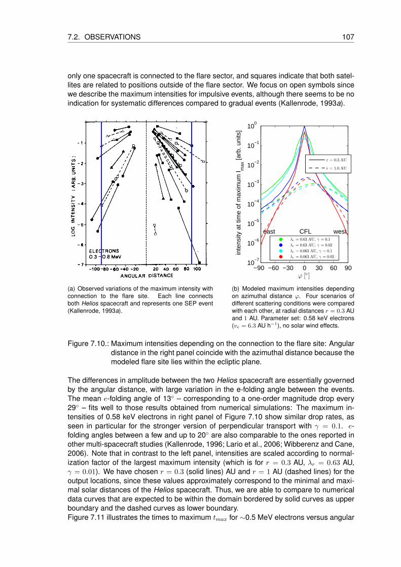
7.2. OBSERVATIONS 107
only one spacecraft is connected to the flare sector, and squares indicate that both satel-lites are related to positions outside of the flare sector. We focus on open symbols sincewe describe the maximum intensities for impulsive events, although there seems to be noindication for systematic differences compared to gradual events (Kallenrode, 1993a).
(a) Observed variations of the maximum intensity withconnection to the flare site. Each line connectsboth Helios spacecraft and represents one SEP event(Kallenrode, 1993a).
−90 −60 −30 0 30 60 9010
−7
10−6
10−5
10−4
10−3
10−2
10−1
100
CFL westeast
ϕ []
inte
nsity
at t
ime
of m
axim
um I m
ax [a
rb. u
nits
]
λr = 0.63 AU, γ = 0.1
λr = 0.63 AU, γ = 0.02
λr = 0.063 AU, γ = 0.1
λr = 0.063 AU, γ = 0.02
r = 0.3 AU
r = 1.0 AU
(b) Modeled maximum intensities dependingon azimuthal distance ϕ. Four scenarios ofdifferent scattering conditions were comparedwith each other, at radial distances r = 0.3 AUand 1 AU. Parameter set: 0.58 keV electrons(ve = 6.3 AU h−1), no solar wind effects.
Figure 7.10.: Maximum intensities depending on the connection to the flare site: Angulardistance in the right panel coincide with the azimuthal distance because themodeled flare site lies within the ecliptic plane.
The differences in amplitude between the two Helios spacecraft are essentially governedby the angular distance, with large variation in the e-folding angle between the events.The mean e-folding angle of 13 – corresponding to a one-order magnitude drop every29 – fits well to those results obtained from numerical simulations: The maximum in-tensities of 0.58 keV electrons in right panel of Figure 7.10 show similar drop rates, asseen in particular for the stronger version of perpendicular transport with γ = 0.1. e-folding angles between a few and up to 20 are also comparable to the ones reported inother multi-spacecraft studies (Kallenrode, 1996; Lario et al., 2006; Wibberenz and Cane,2006). Note that in contrast to the left panel, intensities are scaled according to normal-ization factor of the largest maximum intensity (which is for r = 0.3 AU, λr = 0.63 AU,γ = 0.01). We have chosen r = 0.3 (solid lines) AU and r = 1 AU (dashed lines) for theoutput locations, since these values approximately correspond to the minimal and maxi-mal solar distances of the Helios spacecraft. Thus, we are able to compare to numericaldata curves that are expected to be within the domain bordered by solid curves as upperboundary and the dashed curves as lower boundary.Figure 7.11 illustrates the times to maximum tmax for ∼0.5 MeV electrons versus angular

108 CHAPTER 7. MODEL RESULTS
(a) Time to maximum for ∼0.5 MeV electrons versusconnection angle ϕ. Each line connects both Heliosspacecraft and represents one SEP event (Kallenrode,1993a).
−90 −60 −30 0 30 60 900
1
2
3
4
5
6
7
8
9
ϕ []
time
to m
axim
um t m
ax [h
]
λr = 0.63 AU, γ = 0.1
λr = 0.63 AU, γ = 0.02
λr = 0.063 AU, γ = 0.1
λr = 0.063 AU, γ = 0.02
r = 0.3 AU
r = 1.0 AU
(b) Time to maximum for different azimuthaldistances. Simulation settings are identicalto those defined in Figure 7.10.
Figure 7.11.: Variation of time to maximum with the connection angle (more details cf.text).

7.2. OBSERVATIONS 109
distance. As it has already been done in Figure 7.10, the focus is taken on the sameset of events using the same plotting procedure (except for the semi-logarithmic and nor-malized presentation). The times are separated into three possible categories indicatingwhether the two spacecraft are connected to the flare sector or not (see description in theupper left of each panel in Figure 7.11). Again, there is a clear indication that the time tomaximum increases with increasing angular distance. The slopes become even steeperif one or both spacecraft are separated from the flare site by a neutral line (cf. Section2.2). Of course, sector boundaries can not be modeled by the current model, but nev-ertheless there is no problem in finding an adequate parameter set to fit these times tomaximum (see right panel in Figure 7.11). Whereas the two-point measurements do notallow any analytical description of the azimuthal variations, all scenarios reveal profilesas described by a parabolic function. Obviously, particles need additional time to travelfrom a punctual source to the observer, while particles with good magnetic connection tothe source propagate in field-parallel direction without any cross-field displacements.
(a) Radio burst delays, shown as a function of the magnetic con-nection of IMP 8 to the associated flare for >20 MeV protonevents. IMP-8 is located at r = 1 AU within the Earth’s orbit(Cane and Erickson, 2003).
−90 −60 −30 0 30 60 900
1
2
3
4
5
6
7
8
9
CFL westeast
ϕ []
time
to m
axim
um t m
ax [h
]
λr = 0.24 AU, γ = 0.1
λr = 0.24 AU, γ = 0.02
(b) Modeled time to maximum for differ-ent azimuthal distances. Parameter set:30 keV electrons (corresponding to 56MeV protons with v = c/3 ≈ 2.4 AUh−1), δ-injection in space and time.
Figure 7.12.: Intensity delays varying with connection angle ϕ.
Concerning the angular variations of time-to-maximum intensity of SEP events, Caneand Erickson (2003) also showed that there must be a kind of lateral transport in flar-ing SEP events. SEP events are preceded by type III radio bursts, caused by flaring2 – 50 keV electrons that excite Langmuir waves on the background plasma (see e.g.Baumjohann and Treumann, 1986 or Parks, 1991) which themselves emit electromag-netic waves, whose frequencies depend on the local plasma density. The emission driftsto lower ad lower frequencies as the electrons propagate outward with roughly one third ofthe speed of light. When the electrons reach the spacecraft, no lower emission frequen-cies are observed. For >20 MeV proton events, Cane and Erickson measured the timefrom when the burst started at the Sun to when it reached the local plasma frequency at

110 CHAPTER 7. MODEL RESULTS
r ≈ 1 AU. They plotted these delay times of different events versus the connection angle– the angle between the flare longitude and the footpoint of the field line on which thespacecraft is located (connection angle in the left panel of Figure 7.12).The right panel shows the modeled azimuthal variation of the time to maximum at r = 1AU for two different scenarios. Both scenarios under consideration simulate identicalscattering conditions along the field (λr = 0.24 AU), but they differ in the strength of field-perpendicular diffusive flux. The green line illustrates times for λ⊥ = 0.1 · λ‖ · r2, whereasthe blue line is associated with low perpendicular diffusion (the scaling factor (5.8) isγ = 1/50 instead). Note that tmax has lower values at the western site since cross-fieldtransport additionally shifts particles radially outward. The profiles are still symmetricwithin r = 0.3 AU (not shown in a figure) and resemble those of the simplified, azimuthalmodel by Lampa and Kallenrode (2009). The times are insignificantly overestimatedsince the modeled flare site is located at radial distance r = 0.1 AU. Flare acceleration isexpected to take place in the lower corona at r ≈ 0.01 AU (within 3 solar radii). Due tonumerical reasons, the inner boundary at the CFL was set to r = 0.1 (see Section 7.1).For γ = 1/10 the time of maximum is acquired within less than ten hours for azimuthaldistances of 40 around CFL; it increases to values of a day and more for azimuthal dis-tances beyond 30 for γ = 1/50. For connection angles of ± 90 delay times up to 4 hoursare evident, thus the particles needed additional time to be transported in lateral direc-tion. Using the 2D model, a four hour delay could be reproduced for medium pitch-anglescattering conditions (λr = 0.24 AU), combined with enhanced perpendicular diffusion (γ= 1/10). Thus, cross-field transport could account for what was formerly known as “opencone of propagation” (Lin, 1970) or fast propagation region (van Hollebeke et al., 1975)and what Cane and Erickson (2003) require for the interpretation of the type III radiobursts.
7.2.2. Fitting both intensity- and anisotropy profiles
As seen in the previous Section 7.2.1, the simulation results can qualitatively good de-scribe the SEP intensities at the time of maximum, and the time of the maximum withrespect to the azimuthal distance between the source and the observer. We also haveto validate whether pitch-angle diffusion still works in two dimensions. Can the observeddistributions confirm that the model assumptions are properly chosen? We thereforelooked at four SEP events of relativistic electrons, which have been chosen with respectto the impulsive character. There is no evidence for an interplanetary shock in neitherthe particle nor the plasma data. We have tried to fit the satellite data with the numericalmodel as presented here. We always add some isotropic background plasma in order toconsider the omnipresent background in interplanetary space and to get a reasonable fitto the pre-flare phase. It should be noted that the values differ by at least one order ofmagnitude from the maximum intensities. The pitch-angle distribution will be significantlychanged only if the additional flux lies in the same order of magnitude. This is the case forthe pre-flare phase (the time before anyHαs have been detected) as well as for the phaseof the first arriving particles at the observer’s site. The amount of added nucleon flux aswell as the other fitting values are summarized in Table 7.3 at the end of this section.Figure 7.13 gives an overview about the first three events. Arrows mark the start ofthe flare, as it is interpreted in terms of the Hα emissions. The spatial configurationof the Helios satellites at the measuring time is shown in the insert of each panel inFigure 7.13. The details of the flare and the spacecraft position relative to the flare aregiven in the table below Figure 7.13 with the column “Fpt” indicating the footpoint of

7.2. OBSERVATIONS 111
Figure 7.13.: Intensities of ∼0.5 MeV electrons obtained from Helios 1 (solid lines) andHelios 2 (dotted lines) for April 27, 1979; April 11, 1978; and Dec. 19, 1979(from top to bottom). Intensities are given in [m2 sr s MeV]−1 (Kallenrode,1993a).
Date Flare Hα Helios 1 Helios 2doy Location UT r/AU Fpt ϕ/ r/AU Fpt ϕ/
April 27, 1979 118 N18 E17 0652 0.47 E16 +1 0.36 W30 +47April 11, 1978 101 N22 W56 1410 0.47 E09 -65 0.49 W22 -34Dec. 19, 1979 254 S15 E36 2217 0.62 E23 +13 0.75 W46 +82
Table 7.1.: Three particle events observed by both HELIOS spacecraft.

112 CHAPTER 7. MODEL RESULTS
the observer’s magnetic field line as calculated from the measured solar wind speed(Kallenrode, 1993a), and ϕ being the connection angle between the flare site and thefootpoint. In all three cases, the variation between the spacecraft reflect the combinedeffects of radial and azimuthal variations, however, the events have been selected suchthat the radial influences are not very strong.
Like other numerical simulations before, we are confined to the plane of the ecliptic.However, most of the flare sites are located beyond that layer. Consequently, angulardistances between the flare site and the observer’s magnetic footpoint were projected intothe observer’s plane of H1 and H2. Table 7.1 therefore lists the “azimuthal distances” ϕ,which are slightly smaller than the original angular distances.
In all three events, particle intensities at the spacecraft with the smaller angular separationfrom the flare site (which doubles as the CFL in our model) are much higher and showan earlier and more pronounced maximum as we have already stated in the previousSubsection 7.2.1.
SEP event on April 27, 1979
Concerning the first event on April 27, 1979, it has already been illustrated by Kallenrode(1993a), that both spacecraft are connected magnetically to the flare sector on the solarsurface, with one spacecraft almost on the CFL and the other at an azimuthal distance ofabout 47. Typical differences in the intensity profiles, that have been found in the previ-ous section, can be re-identified: later and smaller maximum intensities for the spacecraftat the larger angular/ azimuthal distance (dashed curve in the top panel of Figure 7.13),although H2 is located slightly closer to the Sun than H1. Moreover, in the late phaseof the event, intensities become similar, leading to “invariant spectra” (see also Section3.2). The same features can be also found in the other two events.
Figure 7.14 shows the simulation results as denoted by solid lines. We added someisotropic background plasma by a constant flow of 3000 nucleons per (m2 s sr MeV).Unfortunately, in the time period around the flare tHα no particles were detected at H1due to instrumental errors. Thus, we were forced to make a crude estimate of the injectionfunction just on the basis of the onset time tHα and of the observations of the remote H2satellite.
The event is fitted by a scenario neglecting solar wind effects (see Figure 7.14). Theparticles’ speed was set to v = 6.3 AU h−1, the ratio of perpendicular-to-parallel diffusionis γ = 0.02. Since the anisotropies at H1 are still non-zero 10 hours after the flare, wechose a slightly gradual injection following the Reid-Axford profile (5.2) with parameters(tdiff , tloss) = (0.5 h, 3 h) at the (projected) location of the flare (solid black curve). Weassume medium scattering conditions with a mean free path of λr = 0.15 AU.
The particle distribution on H2 is almost isotropic as a result of both medium pitch-anglescattering in field-parallel direction as well as diffusion perpendicular to it. The fittedcurves are in good good agreement with the observations, trends and time scales areadequately represented. The fluctuating anisotropy around zero comes from the fact,that there are not enough particles to make statistically relevant averages.
It should be noted that, in general, absolute differences between model and observationdata for the remote spacecraft are overstated visually due to the logarithmic scaling.

7.2. OBSERVATIONS 113
6 8 10 12 14 1610
3
104
105
106
107
tHα time [h]
inte
nsity
[m−
2 s−
1 sr−
1 MeV
−1 ]
Reid-Axford profile for (tdiff = 0.5 h, tloss = 3 h)
Fitted profile for H1
Fitted profile for H2
Data from Helios 1Data from Helios 2
(a) Intensity-time profile
6 8 10 12 14 16−0.5
0
0.5
1
1.5
time [h]
anis
otro
py
tHα
(b) Anisotropy-time profile
Figure 7.14.: Intensities and anisotropies (lower panel) of 0.5 MeV electrons obtainedfrom Helios 1 (blue dots) and Helios 2 (green dots) on April 27, 1979. Thecorresponding solid curves are the fitted profiles according to the followingscenario parameters (for details see text): λr = 0.15 AU , γ = 0.02; and aninjection temporally following a Reid-Axford profile with parameters (tdiff ,tloss) = (0.5 h, 3 h).

114 CHAPTER 7. MODEL RESULTS
13 14 15 16 17 18 19 20 21 22 2310
3
104
105
106
time [h]
inte
nsity
[arb
. uni
ts]
tHα
Fitted profile for H1
Fitted profile for H2
Data from Helios 1Data from Helios 2
(a) Intensity-time profiles
13 14 15 16 17 18 19 20 21 22 23−0.5
0
0.5
1
1.5
time [h]
anis
otro
py
tHα
Fitted profile for H1
Fitted profile for H2
Data from H1Data from H2”Pseudo”-data from H2
(b) Anisotropy-time profiles
Figure 7.15.: Intensity-time and anisotropy-time profiles on April 11, 1978. Data is takenfrom the widely seperated spacecraft Helios 1 and Helios 2. Fitted profilesare indicated by solid lines. Simulation settings: no solar wind effects, λr =0.3 AU (for 0.5 MeV electrons, v = 6.3 AU h−1), γ = 1/10, δ-injection in time,but spatially extended (ϕ = ±50). For details, see text.

7.2. OBSERVATIONS 115
SEP event on April 11, 1978
The SEP event in April 11, 1978, is of different nature, although it qualitatively showsthe same features as those of other multi-spacecraft observations – such as an earlieronset of the first arriving particles and a more pronounced maximum for a detector beingmagnetically closer to the flare site. Both Helios satellites had almost identical radialdistances to the Sun, but were separated by 31 in azimuth (see azimuthal distances inTable 7.1). Kallenrode (1993a) already stated, that the intensities are slightly smaller atthe spacecraft with the larger angular distance (as expected from other multi-spacecraftobservations). However, the electron profiles on both satellites look very similar. Evenafter one and half days after the flare start, the differences in intensities between bothspacecraft are still significant. The profiles tend to become similar on much larger timescales than in the other two ’79 events (see Figure 7.13), where invariant spectra (similarintensities) have already been observed about 12 hours after the start of the flare. OnApril 11th, the intensities still differ by a factor of ten. Locally confined injections can notreproduce the curves, since even small cross-field diffusion with γ = 0.01 smears outsuch strong spatial gradients at ∼0.5 AU within hours. Neither the pronounced maximumintensities nor the almost identical decay slopes could be simulated. We assume, thatboth spacecraft must have been located closer to source particles than to the originalemission site of the Hαs. The SEPs are expected to be transported azimuthally by coronalprocesses, possibly triggered by reconnection. A larger extent of SEPs can also beexplained by the fact, that the flare is located 28 in the north of the ecliptic plane (withthe Helios satellites being inside this plane). Probably, a formerly peak-like distributionexpanded to considerable azimuthal extent until it finally reaches the ecliptic plane.As a consequence, we assume particles to be uniformly injected inside ϕ = ±50 –implying that only Helios 2 is connected to the source region. In principle, such an extentof a particle source could be interpreted as a hydrodynamic shock wave. But as it is saidearlier, a shock can be ruled out because there are no indications neither in the plasmanor the electromagnetic radiation data. Since the anisotropy drops very fast to zero,the diffusion must be very strong: Beeck and Wibberenz (1986) suggested λr ∼ 0.03AU for Helios 2. We choose λr = 0.06 AU inside of the injection cone, and a marginallysmaller value of λr = 0.05 AU beyond. The abruptly rising intensities suggest an impulsiveinjection: the source term was set to a δ-function in time. As seen in Figure 7.15, wecan prevent particles from being distributed equally in azimuth by reducing perpendiculardiffusion by γ = 0.03 and by increasing the intensity gradient in azimuth by the use of aspatially extended source.The delay might be explained in terms of stronger scattering (and weak cross-field diffu-sion) inside the flux tube of Helios 1. The assumption of varying scattering conditions inazimuth is supported by the vanishing anisotropies on Helios 1.Note that because of the lack of magnetic field data, anisotropies on H2 are missingaround tHα . “Pseudo”-anisotropies have been introduced which are computed accordingto the average field of an Archimedean spiral. These “pseudo”-values should be handledwith care or even seriously questioned since they do not consider the variability of thefield. If possible, they should be compared with observed anisotropies shortly beforeand after the time period of missing field data. In particular for this event, the lack ofreliable data is complicated by the fact that the intensities of both the electrons and theprotons (not shown in a figure) suggest a compressed magnetic field at the time of thefirst arriving particles: In a more dense field, the gyro radii (2.2) of SEPs decreases,leading to smaller flux tubes and an enhanced particle flux. This might be the reason why

116 CHAPTER 7. MODEL RESULTS
the observed maximum intensities look more pronounced than the modeled ones.
SEP event on December 19, 1979
The SEP event on December 19, 1979, shows the same features as those of the othermulti-spacecraft observations. The Helios satellites had very similar radial distances tothe Sun, but were widely separated (69 degrees in azimuth, see Figure 7.1). In contrastto the first two events, that have been discussed before, both spacecraft are separated bya neutral line (cf. Section 2.2). Source surface maps of equi-potentials of the magneticfield strength with different polarities indicate that only H1 is connected to the magneticfield sector, in which the flare occurred. The impact of the neutral line on the intensities,especially their extensions down to the photospheric and chromospheric field, may playan important role in particle’s propagation: They can escape along regions of oppositepolarity very fast by additional drift effects (Roelof, 1974; Roelof and Krimigis, 1973). Inaddition, Roelof (1973) showed that intensities and their temporal behavior are differentin different polarity cells. Kallenrode (1993a) already stated that the time to maximumoutside the flare sector increase clearly with angular distance, as seen e.g. in the leftpanel of Figure 7.11. Gold et al. (1973) interpreted these observations in terms of “fastpropagation regions”.And indeed, the assumption of different propagation regions is supported by the fact, thatthe intensities on December 19, are clearly different in at least one order of magnitude un-til they abruptly rise and become similar once H2 encounters the sector boundary aboutone and half days after the flare (see lower panel in Figure 7.13). The change is markedby arrow “A” in the lower panel of Figure 7.13. Concerning the protons, Reinhard (1975)even suggested thatH2 has encountered a different particle population. This thesis couldalso be supported by the first order anisotropies, indicated by the 1-minute resolved dotsin the lower panel of Figure 7.16. Unfortunately, due to the lack of magnetic field dataon H2, we again used the “pseudo”-anisotropies (black dots). The profile indicate thatthe time scales on both spacecraft are very different. On Helios 1 anisotropy drops veryfast to zero, indicating that scattering must be significantly strong. On the other hand, theintensity on H2 remains stationary over hours with high anisotropies. The H1 data canbe interpreted as a nearly scatter-free and gradual event.In order to consider these different propagation regions, we introduce a wide cone of 45
around the injection site, with λr = 0.3 AU and an extended injection of 30 temporallyfollowing the Reid-Axford profile with parameters (tdiff , tloss) = (0.1 h, 0.1 h). Beyondϕ ± 45 λr is assumed to be three times larger. κ⊥
κ‖(r) is scaled by γ = 0.01. The
variation of λr in azimuth gives better numerical results, but they are not yet satisfying:While the profiles for H1 (magnetically connected to the flare sector) properly coincide,the computed anisotropies for H2 are too small and the intensities are slightly higher.The observation can only be reproduced if one additionally assumes SEPs to be emittedby a different source, which is located magnetically closer to the satellite and which isdescribed by a gradual injection function.
SEP event on May 28, 1980
As an example of leveling gradients, Figure 7.18 shows ∼0.5 MeV electrons of the SEPevent on May 28, 1980, between 15 and 24 UT (universal time). The energetic particleswere detected by two spacecraft at different radial distances but closely aligned. Helios 1was located at r = 0.3 AU, while the IMP-8 satellite (Interplanetary Monitoring Platform,
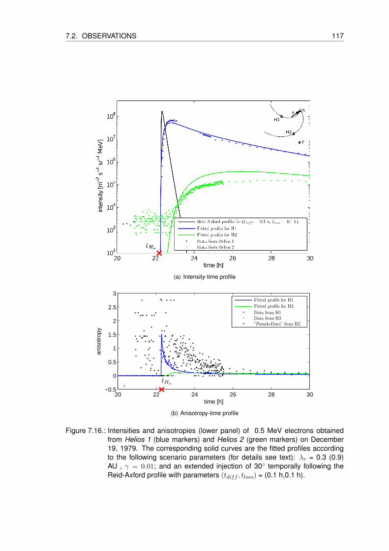
7.2. OBSERVATIONS 117
(a) Intensity-time profile
20 22 24 26 28 30−0.5
0
0.5
1
1.5
2
2.5
3
time [h]
anis
otro
py
tHα
Fitted profile for H1
Fitted profile for H2
Data from H1Data from H2”Pseudo-Data” from H2
(b) Anisotropy-time profile
Figure 7.16.: Intensities and anisotropies (lower panel) of 0.5 MeV electrons obtainedfrom Helios 1 (blue markers) and Helios 2 (green markers) on December19, 1979. The corresponding solid curves are the fitted profiles accordingto the following scenario parameters (for details see text): λr = 0.3 (0.9)AU , γ = 0.01; and an extended injection of 30 temporally following theReid-Axford profile with parameters (tdiff , tloss) = (0.1 h,0.1 h).

118 CHAPTER 7. MODEL RESULTS
Figure 7.17.: Spatial configuration/ topology of the Helios 1, IMP-8 satellites, and the flaresite(s) on May 28, 1980.
IMP 8 MERGE 20sec Resolution Data, 2010) follows a nearly circular orbit around theEarth at a radius of about 35 Earth radii rE . It spends most of its measuring time outsidethe magnetosphere within the solar wind (∼ 60%), and thus it has access to energeticparticles in interplanetary space. Helios 1 was magnetically connected to the flare sitesnear W40 (spatial configuration shown in Figure 7.17), whereas the footpoint of the IMP-8-field line lies at about W105. These values were inferred from the measured solarwind speed of approximately 240 km s−1. The corresponding field lines can be tracedback to the upper corona by the method of backmapping (Nolte and Roelof, 1973).The particle count numbers of both spacecraft cannot be directly compared. First the datais given in different in units: IMP-8 detects particles with dynamic ranges of 1 to 1E+06particles per (cm2 s sr) (IMP 8 MERGE 20sec Resolution Data, 2010), whereas the rawdata of the first Helios satellite is given in units of particles per (m2 s sr MeV) (see e.g.Kallenrode, 1993a). Secondly, the Helios energy band for the electrons is much smaller:0.3 - 0.8 MeV electrons (fraction of the IMP 8 energy band with 0.22 and 2.5 MeV), withspeeds from 5.6 AU h−1 up to 6.6 AU h−1. As a consequence, we additionally haveto rescale the data. SEP measurements haven given enough evidence for an energyspectrum that follows a power law f(E, δ) ∝ E−δ, with exponent δ ranging between 2 and4. By integrating over the energy domain, the center of the distribution within the energydomain [0.3 MeV, 0.8 MeV] can be determined by:
E(δ) =
(∫ 0.8
0.3E f(E, δ)dE
)/
(∫ 0.8
0.3f(E, δ)dE
).
Comparing data sets of different spacecraft including their individual energy bands, thescaling factor is given by:
ζ(δ) =
(∫ 2.5
0.22f(E, δ)dE
)/
(∫ 0.8
0.3f(E, δ)dE
).
Finally, the Helios data set can be compared with the IMP 8 data set via
intensityIMP 8 = ζ(δ = 2) · 1E-04 · E(δ = 2) · intensityH1 ,
with E being the particle’s energy, averaged over the corresponding energy bin.
The final, scaled result can be seen in Figure 7.18: At 0.3 AU, four different events canbe distinguished. All of them are enriched in 3He with 3He/4He ratios ranging between
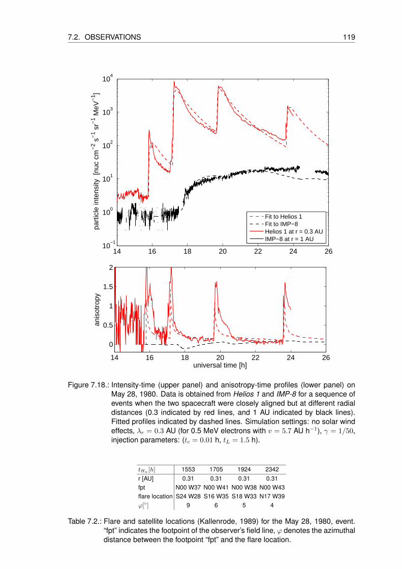
7.2. OBSERVATIONS 119
14 16 18 20 22 24 2610
−1
100
101
102
103
104
part
icle
inte
nsity
[nu
c cm
−2 s
−1 s
r−1 M
eV−
1 ]
Fit to Helios 1Fit to IMP−8Helios 1 at r = 0.3 AUIMP−8 at r = 1 AU
14 16 18 20 22 24 26
0
0.5
1
1.5
2
universal time [h]
anis
otro
py
Figure 7.18.: Intensity-time (upper panel) and anisotropy-time profiles (lower panel) onMay 28, 1980. Data is obtained from Helios 1 and IMP-8 for a sequence ofevents when the two spacecraft were closely aligned but at different radialdistances (0.3 indicated by red lines, and 1 AU indicated by black lines).Fitted profiles indicated by dashed lines. Simulation settings: no solar windeffects, λr = 0.3 AU (for 0.5 MeV electrons with v = 5.7 AU h−1), γ = 1/50,injection parameters: (tc = 0.01 h, tL = 1.5 h).
tHα [h] 1553 1705 1924 2342r [AU] 0.31 0.31 0.31 0.31fpt N00 W37 N00 W41 N00 W38 N00 W43flare location S24 W28 S16 W35 S18 W33 N17 W39ϕ[] 9 6 5 4
Table 7.2.: Flare and satellite locations (Kallenrode, 1989) for the May 28, 1980, event.“fpt” indicates the footpoint of the observer’s field line, ϕ denotes the azimuthaldistance between the footpoint “fpt” and the flare location.

120 CHAPTER 7. MODEL RESULTS
0.1 and 0.2. They are proton poor, and the time scales of the measured soft X-ray andthe Hαs suggest that energetic particles have been released during an impulsive flare.This is supported by the lack of evidence for a passing shock, that would reveal abruptchanges in plasma density, temperature and magnetic field strength for example. Theonly, negligible exception from this is a weak shock from an earlier source passing Helios1 at 1830 UT (see also p. 89 in Kallenrode, 1989).The electromagnetic radiation as well as the intensity and omni-directional anisotropiesreveal similar time profiles. Since, additionally, the flare sites are almost identical, theysupport the assumption of the homology of the events. In these cases, only part of theenergy stored in the magnetic field is released, and the overall field topology is retained(for details see e.g. Gaizouskas, 1983).A different picture of SEP propagation is drawn at 1 AU from the IMP-8 satellite: Pitch-angle scattering is stronger than the focusing effect. While at a radial distance of 0.3AU, the propagation fronts of individual flares are clearly separated from each other, theymerge to a single front with larger time and spatial scales at 1 AU. Cane (2005) alsomade the same comparison and made identical conclusions. This kind of leveling andsmoothing of spatial intensity gradients is exactly what numerical simulations alreadyrevealed, if the observer is not connected to the flare side anymore. Unfortunately, IMP-8gives no information about the angular distributions to support the numerical computedanisotropies. But apart from that: What was formerly explained by a decreasing λr withincreasing radial distance according to slab turbulence (see e.g. Cane, 2005; Wibberenzand Cane, 2006), can also be interpreted by additional cross-field losses without anyradial variability of pitch-angle diffusion.The interpretations and fits to the Helios 1 data set by Kallenrode (1989) showed thatpitch-angle scattering at r = 0.3 AU must be moderate because the anisotropy is highat the time of intensity maximum, and because the anisotropy decays slowly and is stillsignificantly above zero three hours after theHα onsets. Fitting these events by the use ofthe one-dimensional model of focused transport by Roelof (1969a) gave free mean pathsof λr = 0.15±0.05 AU (Kallenrode, 1989, p. 94). Scenarios of the current two-dimensionalmodel with λr ∼ 0.3 AU, an injection onto the CFL following a Reid-Axford profile (5.2) withtime parameters (tloss, tdiff ) =(0.01 h, 1.5 h) and κ⊥-κ‖- ratio being scaled with γ = 1/50can qualitatively reproduce the intensity and omni-directional anisotropy profiles (dashedlines) as well. The latter free mean path is even twice as large as the one fitted by the1D model, although cross-field diffusion leads to a faster removal of particles from theobserver’s site.Four separate δ injections were assumed as it is suggested by the measured intensi-ties at 0.3 AU (see also Kallenrode and Wibberenz, 1991b). A comparison of the max-imum anisotropies shows an adequate fit, but the numerical values subsequently droptoo fast. A more detailed look at the observed anisotropies reveals some subsequentpeak-like flares, whose strength (number of emitted particles) consists of just a fractionof the first flare. These additional particles could explain the long-lasting, gradually fallinganisotropies. This issue can be best seen for the first of the four, strong flares, where adouble-peak structure is evident. It is even more evident in electromagnetic emissions, inparticular in X-ray, microwave and radio data (Kallenrode and Wibberenz, 1991b).SEP simulations at r = 1 AU show that the electron anisotropy varies slowly, rangingbetween 0 and ∼ 0.2. It can even drop below zero. Since only small particle fractions areattributed to that time period, this does not lead to a considerable Sun inward flux. Mostof the time, the anisotropies are at 0.1 or 0.2, because “fresh” particles are supplied bythe series of homologous events. Combined with moderate pitch-angle scattering, IMP-8

7.2. OBSERVATIONS 121
detects slowly varying intensities: The particle flux keeps steady over some hours. Thereis no evidence of separate injections anymore. The numerical results also show that theintensity gradients have almost completely been smoothed.
Date v vsw λr [AU] γ injection background plasma[AU h−1] [km s−1] Helios 1 Helios 2 ∆Φ[] q2(t) q1(s⊥,0) nuc/( m2 s sr MeV)
April 27, 1979 6.3 400 0.15 0.15 δ 150
(0.5 h, 3.0 h) δ 3000April 11, 1979 6.3 460 0.05 0.06 45 3
100δ H 50 7000
Dec 19, 1978 6.3 400 0.3 0.9 45 1100
(0.1 h, 0.1 h) H 30 1875May 28, 1980 5.7 240 0.3 0.3 δ 1
50(0.01 h,1.5 h) δ 3 (H1), 0.75 (H2)
Table 7.3.: Fitting parameters for four ∼0.5 MeV electron events (for details see text).
To sum up the fits to the four impulsive electron events, Table 7.3 gives an overview aboutthe fitting parameters. ∆Φ denotes the azimuthal extent of a certain propagation regionaround the central field line. The corresponding λr is found in the fourth or fifth column,depending on which spacecraft has a better magnetic connection to the injection site. Theambient medium beyond ±∆Φ is characterized by the second free mean path (related tothe other spacecraft). The spatial extent of the source is described by q1(s⊥,0): H 50 e.g.denotes a uniform filling of the field line footpoints within ϕ± 50.Note that due to the lack of sufficient multi-spacecraft data, general conclusions are dif-ficult. But it is evident that SEPs are significantly spread in azimuth on their way tothe observer – even close to the Sun at r = 0.3 AU. Locally confined injections lead tomuch higher intensities with a more pronounced maximum if the spacecraft has a smallerseparation from the flare site. The leveling of gradients can hide multiple consecutiveevents. At least for the events as studied here, the occurrence of sector boundariessignificantly affects field-perpendicular propagation; they might even separate regions ofdifferent propagation properties and different sources. The assumption of λr to be con-stant, κ⊥ to be scaled with r2, and a scaling factor γ ranging between 0.01 and 0.1 hasbeen found reasonable in order to get satisfying fits to the multi-spacecraft observations.
7.2.3. Diffusion as the big leveler vs. sudden flux dropouts
The main objection against diffusive interplanetary transport arises from the abrupt fluxdropouts of flare accelerated particles, as e.g. observed from the ACE spacecraft at r ∼1 AU. It was impossible to model turbulent or abrupt changes in the intensity profiles withthe assumption of λr to be constant in azimuth. On the other hand, Mazur et al. (2000)found spatial structures in scales of an hour or less (see e.g. Figure 7.19). Transientdisturbances such as shocks and magnetic clouds/coronal mass ejections or corotatinginteraction regions (CIRs), caused by the solar wind stream structure, may be possibletriggers. Indeed, some abrupt decreases of electron fluxes could be explained as signa-tures of the disconnection of one end of the cloud’s magnetic field from the solar corona(Larson et al., 1997). But the observed dropouts occur in such large quantities that mag-netic clouds can not explain them solely. Not all dropouts were accompanied by a changein angle of the IMF.Mazur et al. emphasize that according to the plasma data, other acceleration mecha-nisms have to be excluded. Dropouts are said to occur simultaneously at all energies,thus the detected particles are not supposed to be accelerated at traveling shocks. This iswhy Mazur et al. suggested that the spacecraft has changed the position relatively to the

122 CHAPTER 7. MODEL RESULTS
Figure 7.19.: (a) Energy of H-Fe ions (in units of MeV nucleon.1 ) vs. arrival time at 1 AUfor the impulsive flare events of 1999 January 9. (b) H-Fe counts vs. time insmoothed, ∼14 minute bins. (c) Interplanetary magnetic field angle in thegeocentric solar ecliptic (GSE) x-y plane. (d) Interplanetary magnetic fieldangle normal to the GSE x-y plane. Source: (Mazur et al., 2000)
−60 −40 −20 0 20 40 6010
4
105
106
107
108
ϕ []
inte
nsity
[arb
. uni
ts]
t = 1 ht = 5 ht = 10 h
Figure 7.20.: Azimuthal variations of intensity for times t = 1, 5, 10 h. The observer islocated at r= 0.3 AU. The standard scenario (5.1) was chosen, but λr hasbeen reduced to λr = 0.01 AU within a cone of 5 in extent around ϕ = 15.Note that the former azimuthal model has been used (see Section 3.2.2).
7.2. OBSERVATIONS 123
current flux tube and might be subsequently shifted into a neighboring flux tube, whereSEPs are underrepresented. The current model does not allow to change the observer’slocation at a certain field line within a time-series of intensities or anisotropies. But evenif spacecraft motion is involved, the profiles will probably be continuous, since the spatialdiffusion term leads to smooth profiles both in time and space. But small changes of themean free path λr with varying azimuthal distance could lead to significant gradients inthe transition region of different scattering conditions. We have “produced” such a sce-nario in terms of the SEP event on December 19, 1979 (Section 7.2.2). Another exampleis illustrated in Figure 7.20, where a 5 wide cone of enhanced pitch-angle scattering (andconsequently reduced perpendicular diffusion) has been introduced west of the CFL. 10MeV protons, being injected impulsively onto the CFL, are prevented from freely passingthe cone – leading to a considerable intensity gradient of one order of magnitude or moreover just a few degrees in azimuth.Note that the scattering conditions are not only determined by local phenomena, butalso by frozen-in, “fossil” structures that originate from the solar surface. According toMazur et al., a possible scenario would be that the footpoint of a flux tube might becomemixed with the footpoint of another flux tube which is not magnetically connected to anactive region (and consequently still empty). The results would be observed days laterby a remote spacecraft at r = 1 AU in terms of flux dropouts. Note that field-line mixingwas already applied with respect to the field-line-random-walk (FLRW) to estimate theperpendicular diffusion strength with varying radial distance.We assume that the scattering conditions could vary from one flux tube to another. Inliterature, this was already discussed in terms of propagation channels (Borovsky, 2008).Consequently, the first approach would be to change the magnitude of λr (and/ or κ⊥).Another approach would be that the flare will not necessarily be a punctual source func-tion, but an extended one with acceleration efficiencies that might spatially vary. Lampaand Kallenrode (2009) already showed that an extended, uniform source would not af-fect the SEP profiles considerably, “perpendicular diffusion efficiently masks the spatialextend of the injection region”. But will this be still true, when initial particles distributionsdiffer from one flux tube to another? Besides the flux tube varying scattering conditions,this could be a possible explanation of the dropouts in the electron fluxes.


8. Conclusions and Outlook
The main goal of this study was to introduce a numerical model that simulates the prop-agation of solar-flare-accelerated, energetic particles in the inner heliosphere, includingsolar wind effects. Besides the numerical challenges, we checked whether the azimuthalvariations of maximum intensity and time to maximum intensity are of reasonable orderto explain the observations. Simultaneous fits to both intensity- and anisotropy-time pro-files were made in order to estimate the amount of scattering in µ and the strength ofperpendicular diffusion.Inter-model comparisons and comparison of scenarios with differing spatial resolutionsin the validation Chapter 6 have shown, that modeling on varying step sizes lead to good,comparable results. Differences result from inaccuracies in the finite difference terms.Azimuthal resolutions of ∆ϕ = 5 and below are required for possible data fits to take intoaccount the spatially varying propagation properties. The advantage of increasing stepsizes along the magnetic field spiral is found in a better representation of the focusingterm. Moreover, even if the outer boundary of the domain is set far beyond a radialdistance of 3 AU, this leads to no considerable increase in memory allocation.The deficiency can be seen in the requirement of continuous, undisturbed transport co-efficients. This might complicate the simulation of small-scale turbulence, which is im-manent in the perpendicular diffusion coefficient. But we already showed that at leastthe discretization for diffusive term is identical to the one that has been deduced fromGalerkin finite element method (FEM), which uses the alternative integral formulation ofthe PDE. Discontinuities, suggested by flux dropouts observed in low-energetic protons,or traveling shocks, could be probably better integrated. Anyway, fluctuating quantities,which are smaller than the resolution of numerical grid, are leveled off.Concerning the comparison to the observations, we can state that perpendicular diffusionleads to efficient particle spread in azimuth with azimuthal variations in time to maximumand intensity at time of maximum strongly depending on the assumption about the ratioλ⊥/λ|, its radial and energy dependence.The assumption of a ratio λ⊥/λ| between 1/50 and 1/10 at r = 1 AU, and scaled with r2,leads to realistic values for the azimuthal variation of time to maximum and intensity attime of maximum.Secondly, in particular if azimuthal gradients can be maintained (as suggested by theobservations), differences between intensity time profiles on CFL and at some azimuthaldistance can be quite pronounced; in particular the CFL profile might be interpreted interms of weak scattering while the other profiles might be interpreted in terms of diffusivepropagation.Third, the consideration of perpendicular transport in fitting observed intensity and aniso-tropy time profiles therefore would lead to different combinations of injection and meanfree path with larger values of λ on the CFL and smaller values of λ at larger azimuthaldistances. Compared to one-dimensional discretized solution, the free mean path λr canbe chosen lower. Thus, this might help to overcome the magnitude problem (see forinstance Bieber et al., 1994) in the quasi-linear theory.The inclusion of cross-field transport leads to azimuthal variations of time to maximum
125

126 CHAPTER 8. CONCLUSIONS AND OUTLOOK
and intensity at time of maximum comparable with the ones observed in different kinds ofparticle events.This has an interesting consequence for our interpretation of acceleration and injectionmechanisms: the current paradigm is based on the assumption that intensity time profilesreflect the injection from flare and shock onto that field line. Thus it has been assumedthat the shock’s acceleration efficiency can be inferred from these profiles and that theshock is a stronger accelerator close to its nose than at its flanks. Efficient cross fieldtransport will also be effective in the case of the shock being a propagating source ofparticles. Thus profiles at a certain position will be different from the ones expectedfor negligible cross-field transport. Consequently our interpretation of the observationswill be modified – to what extent will only become visible when the shock is included inthis model. In addition, cross-field diffusion also might enhance the shock’s accelerationefficiency by reducing the injection problem. Cross-field diffusion also could account forthe fact that large impulsive events without contribution of a shock can be observed upto ±60 around the flare site without invoking coronal shocks or other mechanisms forcoronal transport.It should be noted that for any given λ‖/λ⊥ the present version of the model underesti-mates the influence of cross-field transport, since perpendicular transport in the merid-ional direction is not considered at all. But a numerical model in a three-dimensionalheliosphere has been introduced by Schwan (2009). It is based on the same code, al-though solar wind effects have not yet been considered.In addition, the presence of magnetic clouds as large-scale magnetic structures alsoaffects particle propagation as does the presence of structures on smaller scales.Fits to observed multi-spacecraft time-profiles could be adequately reproduced, but someevents as well as the presence of flux dropouts suggest, that scattering conditions mightdiffer from one flux tube to another.In sum, this approach suggests that a more detailed understanding of SEP profiles frompoint sources as well as moving sources requires the consideration of this formerly ne-glected effect. Consequently, it is worth developing the model presented here further insuch that both the 3D model and this model including solar wind effect are combined toa single model, that covers the entire inner heliosphere as well as the main propagationprocesses.In addition, upcoming multi-spacecraft measurements (e.g. by STEREO) will provide anew set of particle observations at different positions to test the model in more detail inthe near future.

A. Appendix
A.1. Physical quantities and acronyms
Symbol Dimension Description
α radpitch angle between the particle’s velocity and theoutward tangent to the average magnetic field
AU 149.6E+09 m astronomical unit (distance Sun – Earth)c 3 · 108 m s−1 speed of lightcl+1/2 approximated diffusion coefficient at position zl+1/2
CFLCourant-Friedrich-Levi, or central field line (SEPs areinjected symmetrically around the footpoint of theCFL)
∆ϕ azimuthal distance between two neighboring fieldlines
ε01
µ0c2electric field constant
ε(n)l
truncation error of a finite difference (FD) scheme withrespect to point (tn, xl)
FD finite differenceIMF interplanetary magnetic fieldκµ(r, µ) h−1 pitch-angle diffusion coefficient (PADC)κ‖(r) AU2 h−1 field-parallel diffusion coefficientκ⊥(s‖, s⊥, µ)AU2 h−1 field-perpendicular diffusion coefficientλ|| AU mean free path (mfp) along the field linemfp mean free path
µ cosαcosine of the pitch-angle α, also known as “pitch-cosine”
µ0 4π10−7 N A−2 magnetic field constant
ν ∈ [0, 1]reflection coefficient at the outer boundaries in field-perpendicular direction
ω 0.0103 rad h−1 solar angular speedPDE partial differential equation
Ψ rad bzw. spiral angle (between radial and magnetic field direc-tion of an Archimedean spiral
PADC pitch-angle diffusion coefficient
127

128 APPENDIX A. APPENDIX
Symbol Dimension Description
PADC pitch-angle diffusion coefficient
qspectral index of the power density spectrum of mag-netic fluctuations
QLT quasi-linear theory
r6.955E+08 m =0.004652 AU
solar radius
SEP solar energetic particle
σ Ω−1 m−1conductibility (reciprocal of the specific resistance) ordimensionless polarization of the magnetic field fluc-tuations
sini AUfootpoint of the CFL as arc length along the field line(starting from Sun up to the footpoint)
sinj AUinjection location on the CFL given as arc lengthalong the field line (starting from Sun up to the foot-point)
θ latitude of the Sunvsw 300− 800 km s−1 solar wind speed
A.2. Program details
A.2.1. Structure
The numerical model is based on spatial one-dimensional code by Wong (1982), Schluter(1985), Hatzky (1996) and others. Most of the additional source code was stored withinthe module perpdiff. Comments about the containing subroutines and the variablescan be found in the source code. Additionally, abbreviated information will be given in thissection to ease the introduction into this numerical model. Despite of the modularizationof the newly introduced source code, perpdiff neither is a stand-alone program, nor canit be integrated in the original numerical code of Roelof or Ruffolo model (in contradictionto the former azimuthal scheme by Lampa, 2006). While the former numerical model al-lows differently shaped field lines, the current model is confined to Archimedean spirals.
SUBROUTINE gref
The main program subsequently calls ginout (memory allocation and initializations) gcalc(numerical scheme) and intensi (time-intensity and time-ansotropy profiles).
SUBROUTINE ginout
This routine delegates all memory allocation and initializations, that have almost com-pletely outsourced to the modul perpdiff. It is a skeleton, without the amount of func-tionality, that it originally had.

A.2. PROGRAM DETAILS 129
MODULE perpdiff
The largest source code file contains all global variables, that will be allocated and initial-ized at runtime (static parameters are stored in module parameters). Several subroutinesand functions are provided in order to modularize the work flow and to ease a possibleexpansion of the code. They are invoked by the subroutines ginout and gcalc.
subroutine readInput(infil):It imports the contents of the configuration file infil (see Section A.3) and stores thedata.
subroutine checkinputparameters():It makes plausibility checks to the user’s input.
subroutine calcgridpoints():It computes the numerical grid and its mesh sizes (some essential computations areoutsourced to module perpcalc).
subroutine calcTransportCoefficients():It computes the transport coefficients for almost all transport processes (subroutineginout makes some initializations as well).
subroutine init():It allocates memory needed at runtime; some calculations for the output routines will bedone either.
subroutine setfcorr():It computes the cross sections by numerical integration using the trapezoidal rule; thescheme was improved with regard to varying step sizes along the magnetic field lines(see Section A.4).
subroutine setperpdiffac():The perpendicular diffusion coefficient is set according to Section 5.3.
subroutine setzinjection(dt):The source function Q(t, s‖, s⊥) is set here as a time-varying inner boundary. Its spatialextent around the central field line depends on variable inj_spacial_type, which canbe either “h” (rectangular function), “d” (δ-injection in space) or “g” (Gaussian distribu-tion).
subroutine setperpadvect():It determines the advective flows in field-perpendicular direction.
subroutine free():The routine deallocates memory and closes file streams at the end of the numericalscheme.

130 APPENDIX A. APPENDIX
The following subroutines provide thenumerical scheme for the transport pro-cesses in s‖, s⊥, µ and p, respectively.
subroutinenextRoelofSStep(kk,t,jmax):
Figure A.1.: Source code excerpt ofsubroutine gcalc: Completenumerical scheme.
It contains the field-parallel (s‖) trans-port on varying step sizes: The Lax-Wendroff scheme including a flux lim-iter. Only particles of a fixed energyare involved (denoted by variable kk).t is the current time step index, jmax isthe maximal grid index (beyond jmax noadvective fluxes are computed).
subroutine nextRoelofMuStepL(kk,jmax):It contains the pitch-angle transport(in µ). The input parameters are equiv-alent to those of the above-mentionedsubroutine . Compared to the originalcode, the scheme itself remains un-changed, but all transport coefficients,that hold a spatial dependency, havebeen computed with respect to the dis-torted grid (Figure 3.2).
subroutine nextPStep(jmax)):This routine encapsulates the momen-tum transport scheme (in p). The in-put parameter is equivalent to thoseof the subroutine as mentioned above.Again, the scheme itself remains un-changed, but all transport coefficients,that hold a spatial dependency, havebeen computed with respect to the dis-torted grid and the solar wind refer-ence frame.
subroutine nextperpstep_sw(kk,jmax):This routine holds the perpendicularscheme (in s⊥). The input parameteris equivalent to those of the above-mentioned subroutines. The entire eclip-tic plane is simulated. An alternativeroutine without the extension _sw al-lows cross-field transport with reflect-ing boundaries.

A.2. PROGRAM DETAILS 131
The final part of the subroutine collection in perpdiff are those routines responsible forthe output production:
subroutine getcrossprofile(txt,timestamp,kk):Saves the formatted data of azimuthal intensity- and anisotropy-time profiles at the giventime timestampand momentum pk (k). txtcontains a textual message that will be writ-ten into the header of each output file.
subroutine getGridData(txt,timestepno,timestamp,kk):Saves the unformatted data of pitch-angle distributions for the entire grid (or for thosepoints that correspond to a lower resolution) at the given time timestamp and momen-tum pk (kk). txt contains a textual message that will be written into the header of eachoutput file. The writing process occurs during runtime.
subroutine plot3d(timestepno,kk):The routine is invoked at the end of the numerical scheme. It performs some postprocessing steps to the data, that had been produced by the routine getGridData. In-tensities and anisotropies are computed and are written to a formatted file.
SUBROUTINE gcalc
It contains the complete numerical scheme, the subroutine nextRoelofSStep(kk,t,jmax) ,nextRoelofMuStepL(kk,jmax) , nextPStep(jmax)) and nextperpstep_sw(kk,jmax) arecalled consecutively, the order is given by the summarized approximation method (seeSection 4). Moreover, the output data will be produced here.
SUBROUTINE intensi()
This routine is called after all numerical computations in gcalc have been done (endof the simulation). The temporal evolution of the omnidirectional intensity and first-orderanisotropy will be saved for user-defined locations in file ???PLT.DAT , where ??? denotesthe three-digit scnenario number. The calculations are based on binary raw data of thepitch-angle distribution that has been written out during runtime of the numerical scheme.
A.2.2. Installation
The decision was made to apply the OpenMP API specification for parallel programming(OpenMP Architecture Review Board, 2009) in order to still have proper run times for thisextended 2-dimensional model.The current compiler g95 does not support this standard, thus the open source compilergfortran as part of the GNU compiler collection (GCC) was chosen (GNU Compiler Col-lection, 2010) – even though g95 provides a larger variety of options, better debuggingand more stable compilation results.Whereas the installation under UNIX systems can be done without any severe problems(the GCC is one of the standard libraries), installing under Windows (XP) is not that easy.Again, cygwin as Linux-like environment for Windows systems was applied. It should be

132 APPENDIX A. APPENDIX
noted that the gmp and mpfr packages must be installed for gfortran to work – besidesmake to ease the compilation process.The simulation results might differ when two scenarios run at different platforms sincefloating point numbers and integers are represented by different numbers of bits. Byadditionally setting the flags -fdefault-real-8 and -fdefault-integer-8 during thecompilation, all numbers are set to double precision.This prevents (at least in parts) under- and overflow errors of floating point numbers.These errors occur if not enough bits are provided to represent very high/ low or close-to-zero values.very low values cannot be represented anymore if not enough bits are provided. Butit is also up to the program developer to be aware of multiplication/ divisions of large/small values. For example: Concerning the computation of transport coefficients in per-pendicular direction the order of multiplier had to be chosen properly to get reasonablevalues.After having installed the Cygwin environment including all essential packages as men-tioned above, the following command:
tar -xjvf gfortran-X.X-Cygwin-i686.tar.bz2 -C
will install gfortran in /usr/local/gfortran. Note that the X stands for the current version ofgfortran. Another decompressing, probably graphical user interface (GUI) based tool likeWINRAR could to this job as well.To make this compiler globally reachable, you can then either set /usr/local/gfortran/binto be in the search path or set up a link in your local /bin directory with this command asan example:
ln -s /usr/local/gfortran/bin/gfortran.exe ~/bin/gfortran
Assuming /bin is in your search path, you can invoke gfortran with:
gfortran --version
If the version details of this compiler are shown, the installation is expected to be com-pleted successfully.In order to activate the features of openMP, the additional flag -fopenmp has to be setduring the compilation and the execution process as well. The make utility – that hasbeen applied here – automatizes these processes. Thus, the user must just executesome short commands that have been defined in the accompanying Makefile.To invoke the compilation process which would build all the object files, go into the rootdirectory of the program (e.g. nperpgref/), and then type
make
as bash shell command. Theses files are linked together to the executable gref.exe,which will be started by
make run

A.2. PROGRAM DETAILS 133
Figure A.2.: Fork-Join model of parallel execution, OpenMP Architecture Review Board(2009).
All the results from the compilation process will be stored in the sub-folder bin/. Thesimulation results can be found at dat/. All these outputs can deleted by the command
make clean ,
whereas
make dclean
would delete the simulation data only. Note that the files are irreversibly deleted andcannot be restored.The configuration input file can be manipulated by the separate program para.
make para
The resulting executable is para.exe. Note that the additional parameters for 2-dimensionaltransport can not be restored, but they can be appended manually by the correspondinglines that have been saved in a separate copy file. Normally, it is more comfortable to dochanges in this config file by hand. Changes with respect to the PADC should be donewith this tool with priority.
A.2.3. Parallelization
The OpenMP API may be used to direct multi-threaded, shared memory parallelism ex-plicitly. OpenMP (Open specifications for Multi-Processing) provides a portable, scalablemodel. The API supports C/C++ and Fortran on multiple architectures, including UNIXand Windows NT.The original program was serial, so there was always one single execution step afteranother and all steps were executed consecutively. Giving up serialization in terms ofthis multi-dimensional summarized approximation method is not easy since – during adefinite transport process – all other variables of the phase space density have to be keptconstant.This is why the regions, where multiple threads can work (parallel regions, see FigureA.2), have to start/end where these individual transport process start/end. Since OpenMPis an explicit (not automatic) programming model, the programmer has to decide whereto fork the master thread and where to join it.
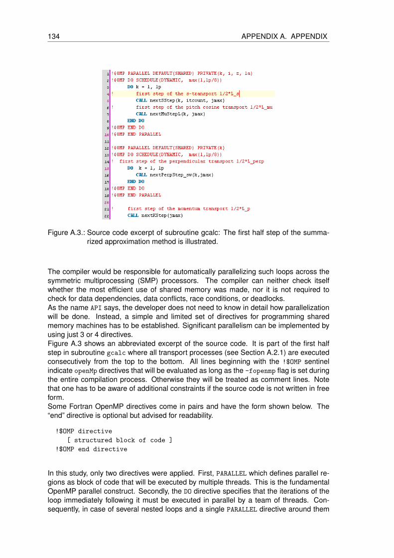
134 APPENDIX A. APPENDIX
Figure A.3.: Source code excerpt of subroutine gcalc: The first half step of the summa-rized approximation method is illustrated.
The compiler would be responsible for automatically parallelizing such loops across thesymmetric multiprocessing (SMP) processors. The compiler can neither check itselfwhether the most efficient use of shared memory was made, nor it is not required tocheck for data dependencies, data conflicts, race conditions, or deadlocks.As the name API says, the developer does not need to know in detail how parallelizationwill be done. Instead, a simple and limited set of directives for programming sharedmemory machines has to be established. Significant parallelism can be implemented byusing just 3 or 4 directives.Figure A.3 shows an abbreviated excerpt of the source code. It is part of the first halfstep in subroutine gcalc where all transport processes (see Section A.2.1) are executedconsecutively from the top to the bottom. All lines beginning with the !$OMP sentinelindicate openMp directives that will be evaluated as long as the -fopenmp flag is set duringthe entire compilation process. Otherwise they will be treated as comment lines. Notethat one has to be aware of additional constraints if the source code is not written in freeform.Some Fortran OpenMP directives come in pairs and have the form shown below. The“end” directive is optional but advised for readability.
!$OMP directive
[ structured block of code ]
!$OMP end directive
In this study, only two directives were applied. First, PARALLEL which defines parallel re-gions as block of code that will be executed by multiple threads. This is the fundamentalOpenMP parallel construct. Secondly, the DO directive specifies that the iterations of theloop immediately following it must be executed in parallel by a team of threads. Con-sequently, in case of several nested loops and a single PARALLEL directive around them

A.3. USER INTERFACES 135
(parallel region has already been initiated), the inner loops will be treated as serial code.
The DEFAULT clause allows the user to specify a default scope for all variables in thelexical extent of any parallel region. Here, as default, all variables will be shared. ThePRIVATE(...) statement lists all variables that are private to each thread; each threadwill have its own unique copy. Besides the private declarations, other possible read/writeconflicts have been resolved explicitly by extending all writable variables or array withinparallel regions to an extra dimension – with each additional entry been related to aspecific thread.The SCHEDULE(type,chunk) clause describes how iterations of the loop are divided amongthe threads in the team. The default schedule is implementation dependent. As type ,DYNAMIC was chosen: Loop iterations are divided into pieces of size chunk , and sched-uled dynamically among the threads; when a thread finishes one chunk, it is dynamicallyassigned to another. According to the source code, the default chunk size is lp/8.As seen in the source code in Figure (A.1) both field-parallel transport in s and pitch-angle scattering in µ will be executed in parallel with respect to momentum/ particle speed(lp grid points). The reason for this single parallel region is that both tranport schemesdo not depend on velocity.The cross-field transport had to be parallelized separately since the transport directionchanges. Otherwise, a complete parallelization would lead to read/write conflicts whenboth parallel and perpendicular transport schemes try to get access to identical phasespace density cells ξj,l.The numerical scheme for momentum transport nextKStep(jmax) has been parallelizedaccording to number of field lines llong (even if it is not indicated in Figure A.1). All par-ticle velocities have to be computed for the next (half) time step before the new positionsdue to parallel advection along the IMF lines can be set.
A.3. User interfaces
The configuration file contains all parameters needed for a complete setup of the numer-ical model. The first 40 lines are identical to those of the original configuration file, that isused for the one-dimensional models of the Roelof’s and Ruffolo’s equation. In contrastto the former models, the parameter choice lacks in some alternatives, which will be il-lustrated in this section. The standard user will not be forced to make direct changes inthe source code, but if he wants to, Section A.2.1 will give some insight into the programstructure.
Line 1 denotes a 56-character-long string of a simple comment that will be written intothe output files. Their names are given in the following three lines. The first three char-acters of each file should be identical (and a number), because they correspond to thescenario number. The first file records almost all parameter settings including additionalcomments. The second contains time-series of pitch-angle distributions at different loca-tions. The third is filled with coefficients up to fourth order of Legendre polynomials, thatwill be fitted to the pitch-angle distributions along the central field line (CFL). The data willbe saved at the end of the simulation.Each of the two characters in line 5 has its own relevance: The first letter can be “S”or “W”. By the use of “S”, the numerical value of the pitch-angle diffusion coefficient(PADC) will be determined by the theory of slab turbulence (see Section 2.4.2). The

136 APPENDIX A. APPENDIX
corresponding parameters are located in the following line: with the number of pitch-angles mmu, the spectral index q, the resonance gap H and the polarization σ. If the firstletter in line 4 is set to “W”, the user has to define the PADC manually. The second letterin line 4 will be a flag for the program to decide how the PADC should be adapted to thenumericalscheme. If it is “J” and the user decides to take the slab-PADC, the Integro-interpolationwill be applied (see Section 4.3). Manually defined PADCs will be changed by a simplelinear interpolation. In case of an “N” (instead of “J”) no adjustments to the PADC will bedone.The next two following parame-
jEdit - configfile.dat
09.02.10 18:46 :: page 1
1 1.0 MeV Protons lambda = 0.1 AU
2 001GRF.DAT
3 001BIN.DAT4 001001.DAT
5 SJ
6 40 1.600000 0.0000000E+00 0.0000000E+00
7 10.08 1.0
9 a
10 0.1013138 0.2870357 0.4506869 0.5928327 0.7140370
11 0.8148608 0.8958582 0.9575721 1.000528 1.025222 12 1.032111 1.021586 0.9939403 0.9493110 0.8875782
13 0.8081763 0.7096978 0.5889324 0.4378706 0.2276414
14 0.2276414 0.4378706 0.5889324 0.7096978 0.8081763
15 0.8875782 0.9493110 0.9939403 1.021586 1.032111 16 1.025222 1.000528 0.9575721 0.8958582 0.8148608
17 0.7140370 0.5928327 0.4506869 0.2870357 0.1013138
18 0.0000000E+00 0.1969471 0.3715382 0.5243405 0.6559151
19 0.7668259 0.8576279 0.9288723 0.9810895 1.014791 20 1.030455 1.028496 1.009257 0.9729536 0.9195790
21 0.8487823 0.7595488 0.6495001 0.5127925 0.3293884
22 9.1113508E-02 0.3293884 0.5127925 0.6495001 0.7595488
23 0.8487823 0.9195790 0.9729536 1.009257 1.028496 24 1.030455 1.014791 0.9810895 0.9288723 0.8576279
25 0.7668259 0.6559151 0.5243405 0.3715382 0.1969471
26 0.0000000E+00
27 0.328 2
29 7.5
30 4
31 5.0000001E-02 0.7000000 0.8000000 0.9000000 1.15000
32 1.57000 60.00000
33 -0.5000000 0.5000000 1.000000 0.5000000 2.142857
34 2.142857 2.142857
35 1.00000036 0.0000000 0.0000000 0.0000000E+00
37 1
38 1.5708 400.0000
39 0.0000E+00 0.000000E+0040 1
41 0.01 # ds
42 1E+11 d 10.0 # mass0, inj_spacial_type, inj_spacial_param
4344 5.0 1 72 1.0 5.0 # dz, llatt, llong, zfrac, dz_resolution
45 1 # projection_type
46 2 # nout
47 0.30 48 -90.00
49 0.00
50 11 # twatch
51 0.1 1.0 2.0 3.0 4.0 5.0 6.0 7.0 8.0 9.0 10.0 # t52 6 # rn
53 0.1 0.3 1.0 1.5 2.0 3.0 # routs
54 32 # lp
55 0.1
Figure A.4.: Configuration file
ters are the simulation period inhours (line 7) and the particlespeed given in AU h−1. Note thatthis parameter becomes redun-dant if the momentum transportis explicitly switched on (for de-tails see comments to line 52).The letter “a” in line 9 determinesthe IMF’s shape to be Archimedean(Parker) spiral. The shape de-pends on both inclination of theecliptic plane and the solar windspeed given in km s−1; these val-ues can be found at line 38. Thesolar angular speed ω = 0.0103rad h−1, which is also responsi-ble for the shape, is assumed tobe independent of the latitude. Theparameter “a” is not allowed to bechanged, since there is no alter-native to the Archimedean spiralat present. Changes would leadto malfunctions of the program.Lines 10-17 contain the discretizedPADC. Lines 18-26 also containthe interpolation values for the PADC,but they are computed accordingto a pitch-angle grid, that is shiftedby half step size. This results inan additional PADC value definedwithin the interval µ ∈ [−1,+1].Line 27: The first location at the CFL given in arc length along the field line. Additionallocations can be specified inlines 46 – 49: Line 46 is set to 1 by default. Thus, at least a single observation point isnecessary for a valid run. The following line denotes the arc length of additional locations,line 48 names the azimuthal distances of the observation points (the CFL is located atϕ = 0) and line 49 gives the latitudinal information. Here, the latitudes are set to 0 –indicating that interplanetary transport is confined to the epliptic plane only.Line 28 gives the spatial dependency ns of the PADC. By default, ns = 2 is chosen such
A.3. USER INTERFACES 137
that λr = const. is fulfilled. Other choices are possible, for example such that the spatialdependencies are given by the 7 spatial nodes in line 31 – 32 and the correspondingstrength of the PADC (lines 33 – 34). It should be noted that the latter node (line 32, lastnumber) also denotes the outer boundary of the CFL. When the simulated particles reachthe outer boundary in field-parallel direction, they are allowed to be reflected towards theSun. The reflection coefficient is located in line 35 and is set to 1 by default (full reflection).
The magnetic field can be modified locally to realize a magnetic bottle. Its strength andextent parameters can be found at line 36.
Line 37: The number 1 indicates that all the output data (pitch-angle distributions) will bewritten for each time, higher values, e.g. 100, means that only each 100th data value willbe written.
So far, all parameters have been elucidated that have already found their application informer models. The additional parameters are:
At line 41: The spatial step size ∆s along the field lines. Note that constant step sizesare not allowed anymore. Any value of ∆s will be ignored by the program. However, thisparameter has been preserved, so that the configuration file can be still applied to boththe original program gref and the azimuthal model quergref.
Line 42: Source parameters: Total mass of particles m0, injection type (“d”: δ-injection,“h”, rectangular injection, “g”, Gaussian injection) and the spatial extent of the source.
Line 44: From left to right: Azimuthal resolution given in degrees, number of field linesin latitudinal direction (only “1” will be accepted), number of field lines in azimuthal direc-tion, reflection coefficient in field-perpendicular direction (see also Section 4.6) and theazimuthal resolution for the output data (given in degrees).
Line 45: The integer is relevant to the cross-field profiles. “1” denotes slices through theecliptic plane; “2” is expected to be slice perpendicular to it, with the CFL placed in thecenter. The parameter becomes important when spatial 3D interplanetary transport willbe simulated in the near future.
Line 50 – 51: Number of snapshots of the ecliptic plane and the azimuthal profiles, aswell as a list of times when these snapshots will be taken.
Lines 52 – 53: Azimuthal cross-field profiles: The first parameter denotes the number ofslice through the plane, and the list in the following line gives the corresponding radialdistances.
Line 52: Number of nodes for momentum transport lp. If lp= 0, momentum transportwill be switched off, and particles will have the speed as defined in line 8. Otherwise, thevelocities will be computed according to (4.31).
Line 55: Ratio between the perpendicular and parallel diffusion coefficient γ, scaled withr2.
In order to manipulate the pitch-angle diffusion coefficient values, it is recommendedto use the stand-alone program para (Section A.2.2), because these numbers need tobe processed further to be well tolarable to the numerical scheme (Section 4.3). Theremaining scalar values can be changed by hand as well.

138 APPENDIX A. APPENDIX
0 1 2 30
5
10
15
20
r [AU]
L(r)[AU
−1]
(a) inverse focusing length in an idealizedArchimedean field
0 1 2 30
50
100
150
200
250
r / [AU]
fluxtubecrosssectionA(r)/km
2
refined trapeziodal rule
classical trapeziodal rule
cell cross section Ac(r) = A0,c ∆s⊥(r)r∆ϕ
analyt. solution A(r) = A0r2(1 + ω⊙ sin (θ) v−1
sw )−0.5
(b) flux tube cross sections
Figure A.5.: Numerical computation of the flux tube cross sections by means of the fo-cusing length.
A.4. Cross sections of flux tubes and their numericaltreatment
Both, the computational implementation of the Roelof’s equation and the Ruffolo equationcalculate the cross sections numerically by using the simple trapezoidal rule for equallyspaced abscissas (Press et al. (1992), p. 124-129).Applying a numerical treatment was necessary since the above-mentioned integrationscheme is not accurate enough to describe the cross sections satisfyingly - especiallywhen step sizes become too large. Since L(s)−1 is a monotonously decreasing function(see left panel in FigureA.5), an numerical integration over the inverse focusing lengthwould be overestimated compared to a possible analytical solution (right panel in FigureA.5). As in all numerical integration schemes, the truncation error sums up along theintegration path. Consequently, the computed cross sections already show a significantdeviation beyond 1 AU compared to the analytical solution.Thus we refined the scheme by introducing virtual grid points between the already existinggrid points. Thus we made an adoption from the extended formula of the trapezoidal rule(Press et al. (1992), p. 127), but used varying step sizes instead.Note that these virtual points themselves do not contribute to the numerical transportscheme but are solely computed in order to get accurate flux tube values.
Cross sections are determined this way:
A(s) = A0(s) exp
(∫1
L(s)ds
), (A.1)
with A0(s) being the cross section at the footpoint of the field line, and L(s) being thefocusing length (3.7). The relation is a direct consequence of the fact that particles for aflux rope length unit are conserved and also of the Gaussian Law (the magnetic flux has

A.4. NUMERICALLY SOLVED FLUX TUBES 139
to be conserved within a flux tube, valid for the both transport equations, see also Hatzky(1996), p. 42). In case of the idealized, IMF forming Archimedean spiral field (constantsolar wind and no further magnetic disturbances are assumed), the analytical solution ofthe cross section is:
A(r) =A0r
2
B0
√1 + ωr sin θv−1
sw
, (A.2)
which is the multiple of the inverse of the magnetic field strength. In these studies, thecross sections at the footpoint of each field line have been set to:
A(r = r0) = ∆s⊥(r).
Consequently, we have not made any assumption about the geometry in meridional di-rection. Any other cross sections beyond r0 are directly computed according to the localmagnetic field strength B(r). They differ solely in a constant whose value is given bycross section size and the magnetic field strength at the footpoints. Note that the crosssections could alternatively be calculated by simply taking the product of ∆s⊥(r) · r∆θ.The second factor approximately describes the ”height” of a cell in meridional direction,which is simply the arc-length on a circle with radius r and angular displacement ∆θ to theneighboring field line. As it is shown on the right hand side of Figure A.5, these cell crosssections are well fitted to the red-colored analytical solution (in this case, θ and ϕ areidentical). But nevertheless, we decided to work the refined trapezoidal rule in order toaccommodate magnetic disturbances ranging from the stream structure of the interplan-etary medium over transient disturbances such as shocks and magnetic clouds/coronalmass ejections.

140 APPENDIX A. APPENDIX
A.5. Various intensity-time profiles for ∼0.5 MeV electrons
For a parameter study, the mean free path λr has been varied by λr = 0.063, 0.63 and 6.3AU. Moreover, the ratio of the perpendicular to the parallel diffusion was set to γ =0.02and 0.1 at r = 1 AU, and scaled with r2 as it is assumed in the standard scenario. Theresulting six intensity-time- and anisotropy-time profiles are plotted and arranged side-by-side in this subsection to get a more detailed look into the dynamics of the modeled two-dimensional diffusion. All the features such as vanishing gradients, negative anisotropies,variations in azimuth together with some of these figures have already been discussedin Section 7.1. The focus is taken on ∼0.5 MeV electrons whose data was obtained atdifferent radial distances (r =0.3 and 1.0 AU) as well as different azimuthal distancesfrom the central field line. SEPs are injected impulsively onto the footpoint of the CFL,described formally as a Dirac-delta function. The simulation results do not provide anynew features but they add 10-hour-data for wide domain of parameter sets.
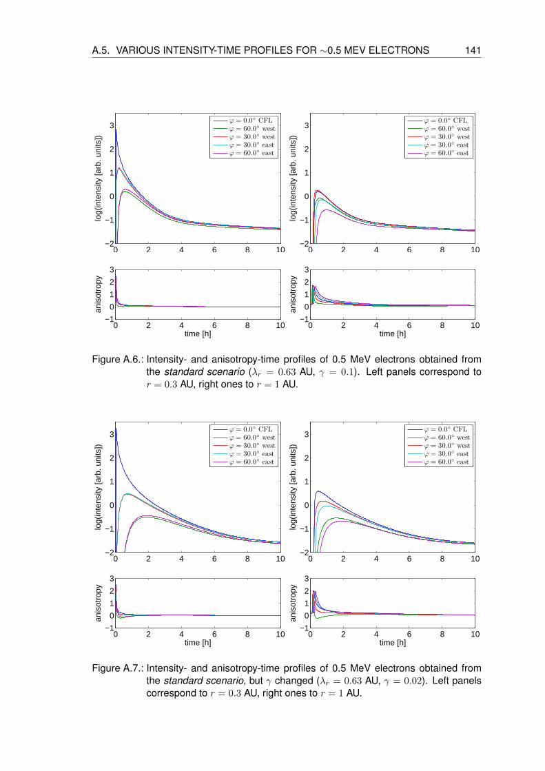
A.5. VARIOUS INTENSITY-TIME PROFILES FOR ∼0.5 MEV ELECTRONS 141
0 2 4 6 8 10−2
−1
0
1
2
3
log(
inte
nsity
[arb
. uni
ts])
ϕ = 0.0 CFLϕ = 60.0 westϕ = 30.0 westϕ = 30.0 eastϕ = 60.0 east
0 2 4 6 8 10−2
−1
0
1
2
3
log(
inte
nsity
[arb
. uni
ts])
ϕ = 0.0 CFLϕ = 60.0 westϕ = 30.0 westϕ = 30.0 eastϕ = 60.0 east
0 2 4 6 8 10−1
0
1
2
3
time [h]
anis
otro
py
0 2 4 6 8 10−1
0
1
2
3
time [h]
anis
otro
py
Figure A.6.: Intensity- and anisotropy-time profiles of 0.5 MeV electrons obtained fromthe standard scenario (λr = 0.63 AU, γ = 0.1). Left panels correspond tor = 0.3 AU, right ones to r = 1 AU.
0 2 4 6 8 10−2
−1
0
1
2
3
log(
inte
nsity
[arb
. uni
ts])
ϕ = 0.0 CFLϕ = 60.0 westϕ = 30.0 westϕ = 30.0 eastϕ = 60.0 east
0 2 4 6 8 10−2
−1
0
1
2
3
log(
inte
nsity
[arb
. uni
ts])
ϕ = 0.0 CFLϕ = 60.0 westϕ = 30.0 westϕ = 30.0 eastϕ = 60.0 east
0 2 4 6 8 10−1
0
1
2
3
time [h]
anis
otro
py
0 2 4 6 8 10−1
0
1
2
3
time [h]
anis
otro
py
Figure A.7.: Intensity- and anisotropy-time profiles of 0.5 MeV electrons obtained fromthe standard scenario, but γ changed (λr = 0.63 AU, γ = 0.02). Left panelscorrespond to r = 0.3 AU, right ones to r = 1 AU.

142 APPENDIX A. APPENDIX
0 2 4 6 8 10−2
−1
0
1
2
3
log(
inte
nsity
[arb
. uni
ts])
ϕ = 0.0 CFLϕ = 60.0 westϕ = 30.0 westϕ = 30.0 eastϕ = 60.0 east
0 2 4 6 8 10−2
−1
0
1
2
3
log(
inte
nsity
[arb
. uni
ts])
ϕ = 0.0 CFLϕ = 60.0 westϕ = 30.0 westϕ = 30.0 eastϕ = 60.0 east
0 2 4 6 8 10−1
0
1
2
3
time [h]
anis
otro
py
0 2 4 6 8 10−1
0
1
2
3
time [h]
anis
otro
py
Figure A.8.: Intensity- and anisotropy-time profiles of 0.5 MeV electrons obtained fromthe standard scenario, but λr changed (λr = 0.063 AU, γ = 0.1). Left panelscorrespond to r = 0.3 AU, right ones to r = 1 AU.
0 2 4 6 8 10−2
−1
0
1
2
3
log(
inte
nsity
[arb
. uni
ts])
ϕ = 0.0 CFLϕ = 60.0 westϕ = 30.0 westϕ = 30.0 eastϕ = 60.0 east
0 2 4 6 8 10−2
−1
0
1
2
3
log(
inte
nsity
[arb
. uni
ts])
ϕ = 0.0 CFLϕ = 60.0 westϕ = 30.0 westϕ = 30.0 eastϕ = 60.0 east
0 2 4 6 8 10−1
0
1
2
3
time [h]
anis
otro
py
0 2 4 6 8 10−1
0
1
2
3
time [h]
anis
otro
py
Figure A.9.: Intensity- and anisotropy-time profiles of 0.5 MeV electrons obtained fromthe standard scenario, but λr and γ changed (λr = 0.063 AU, γ = 0.02). Leftpanels correspond to r = 0.3 AU, right ones to r = 1 AU.
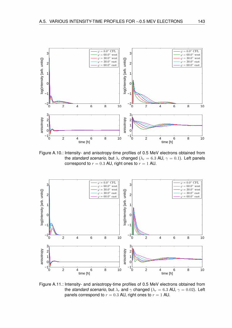
A.5. VARIOUS INTENSITY-TIME PROFILES FOR ∼0.5 MEV ELECTRONS 143
0 2 4 6 8 10−2
−1
0
1
2
3
log(
inte
nsity
[arb
. uni
ts])
ϕ = 0.0 CFLϕ = 60.0 westϕ = 30.0 westϕ = 30.0 eastϕ = 60.0 east
0 2 4 6 8 10−2
−1
0
1
2
3
log(
inte
nsity
[arb
. uni
ts])
ϕ = 0.0 CFLϕ = 60.0 westϕ = 30.0 westϕ = 30.0 eastϕ = 60.0 east
0 2 4 6 8 10−1
0
1
2
3
time [h]
anis
otro
py
0 2 4 6 8 10−1
0
1
2
3
time [h]
anis
otro
py
Figure A.10.: Intensity- and anisotropy-time profiles of 0.5 MeV electrons obtained fromthe standard scenario, but λr changed (λr = 6.3 AU, γ = 0.1). Left panelscorrespond to r = 0.3 AU, right ones to r = 1 AU.
0 2 4 6 8 10−2
−1
0
1
2
3
log(
inte
nsity
[arb
. uni
ts])
ϕ = 0.0 CFLϕ = 60.0 westϕ = 30.0 westϕ = 30.0 eastϕ = 60.0 east
0 2 4 6 8 10−2
−1
0
1
2
3
log(
inte
nsity
[arb
. uni
ts])
ϕ = 0.0 CFLϕ = 60.0 westϕ = 30.0 westϕ = 30.0 eastϕ = 60.0 east
0 2 4 6 8 10−1
0
1
2
3
time [h]
anis
otro
py
0 2 4 6 8 10−1
0
1
2
3
time [h]
anis
otro
py
Figure A.11.: Intensity- and anisotropy-time profiles of 0.5 MeV electrons obtained fromthe standard scenario, but λr and γ changed (λr = 6.3 AU, γ = 0.02). Leftpanels correspond to r = 0.3 AU, right ones to r = 1 AU.


Bibliography
Alfven, H. (1976), “On frozen-in field lines and field line reconnection”, J. Geophys.Res. , Vol. 81, pp. 4019–4021.
Anderson, D., Tannehill, J. and Pletcher, R. (1984), Computational Fluid Dynamics andHeat Transfer, Series in Computational Methods in Mechanics and Thermal Sciences,Hemisphere Publishing Corporation, pp. 27–28, 159.
Baumjohann, W. and Treumann, R. (1986), Basic space plasma physics, Imperial CollegePress, London.
Beeck, J., Mason, G., Hamilton, D., Wibberenz, G., Kunow, H., Hovestadt, D. and Klecker,B. (1987), “A multispacecraft study of the injection and transport of solar energeticparticles”, Astrophys. J. , Vol. 322, pp. 1052–1072.
Beeck, J. and Wibberenz, G. (1986), “Pitch angle distributions of solar energetic particlesand the local scattering properties of the interplanetary medium”, Astrophys. J. , Vol.311, p. 437.
Bieber, J., Earl, J., Green, G., Kunow, H., Muller-Mellin, R. and Wibberenz, G. (1980),“Interplanetary pitch angle scattering and coronal transport of solar energetic particles:New information from helios”, J. Geophys. Res. , Vol. 85, p. 2313.
Bieber, J., Matthaeus, W., Shalchi, A. and Qin, G. (2004a), “Nonlinear guiding centertheory of perpendicular diffusion: General properties and comparison with data”, Geo-phys. Res. Lett. , Vol. 31, p. L10805.
Bieber, J., Matthaeus, W., Shalchi, A. and Qin, G. (2004b), “Nonlinear guiding center the-ory of perpendicular diffusion: General properties and comparison with observation”,Geophys. Res. Lett. , Vol. 31, p. L10805.URL: http://www.agu.org/pubs/crossref/2004/2004GL020007.shtml
Bieber, J., Matthaeus, W., Smith, C., Wanner, W., Kallenrode, M.-B. and Wibberenz,G. (1994), “Proton and electron free mean paths: The palmer consensus revisited”,Astrophys. J. , Vol. 420, p. 303.
Borovsky, J. (2008), “Flux tube texture of the solar wind: Strands of the magnetic carpetat 1 AU ?”, J. Geophys. Res. , Vol. 113, p. A08110.
Bronstein, I., Semendjajew, K., Musiol, G. and Muling, H. (1993), Taschenbuch der Math-ematik, Harri Deutsch, Frank am Main.
Burlaga, L. (1991), Magnetic clouds, in R. Schwenn and E. Marsch, eds, ‘Physics of theInner Heliosphere’, Vol. 2, Springer, Berlin, p. 1.
Cane, H. (2005), Are there direct flare particles in large solar particle events ?, in H. La-coste, ed., ‘Solar Wind 11 – SOHO 16 Connecting Sun and Heliosphere’, Vol. ESASP-592, ESA Publications Division, pp. 71–74.
145

146 Bibliography
Cane, H. and Erickson, W. (2003), “Energetic particle propagation in the inner helio-sphere as deduced from low-frequency (< 100 kHz) observations of type III radiobursts”, J. Geophys. Res. , Vol. 108, p. 1203.
Chattot, J.-J. (2002), Computational Aerodynamics and Fluid Dynamics, Springer-VerlagBerlin Heidelberg.
Compton, A. and Getting, I. (1935), “An apparent effect of galactic rotation on the intensityof cosmic rays”, Phys. Rev. , Vol. 47, p. 817.
Crank, J. and Nicolson, P. (1947), “A practical method for numerical evaluation of solu-tions of partial differential equations of the heat-conduction type”, Vol. 43, Proc. Camb.Phil. Soc., pp. 207–226.
Dalla, S., Balogh, A., Krucker, S., Posner, A., Muller-Mellin, R., Anglin, J., Hofer, M.,Marsden, R., Sanderson, T., Tranquille, C., Heber, B., Zhang, M. and McKibben, R.(2003), “Properties of high heliolatitude solar energetic particle events and constraintson models of acceleration and propagation”, J. Geophys. Res. , Vol. 30, p. 8035.
Denskat, K., Beinroth, H. and Neubauer, F. (1983), “Interplanetary magnetic field powerspectra with frequencies from 2.4·10−5 Hz to 470 Hz from Helios-observations duringsolar minimum conditions”, J. Geophys. Res. , Vol. 6, p. 2215.
Diehl, R., Parizot, E., Kallenbach, R. and von Steiger, R., eds (2002), The astrophysicsof galactic cosmic rays, Kluwer, Dordrecht.
Droge, W. (1993), “Transport of solar energetic particles”, Ap. J. S. , Vol. 90, pp. 567–576.
Dwivedi, B. (2003), The solar corona, in H. Antia, A. Bhatnagar and P. Ulmschneider, eds,‘Lectures on Solar Physics’, Vol. ESA SP-592, Springer, Berlin, Heidelberg, p. 281.
Dwyer, J., Mason, G., Mazur, J., Jokipii, J., von Rosenvinge, T. and Lepping, R. (1997),“Perpendicular transport of low energy corotating interaction region - associated nu-clei”, Astrophys. J. , Vol. 490, p. L115.
Eddington, A. (1926), The internal constitution of the stars, Cambridge University Press.
Farlow, S. (2003), Partial Differential Equations for Scientists and Engineers, Dover Pub-lications, Inc, New York.
Fisk, L. and Axford, W. (1968), “Effect of energy changes in solar cosmic rays”, J. Geo-phys. Res. , Vol. 73, p. 4396.
Fisk, L. and Axford, W. (1969), “Anisotropies of solar cosmic rays”, Sol. Phys. , Vol. 7,p. 486.
Forbush, S. (1946), “Three unusual cosmic ray increases possibly due to charged parti-cles from the Sun”, Phys. Rev. , Vol. 70, p. 771.
Gaizouskas, V. (1983), “The relation of solar flares to the evolution and proper motion ofmagnetic fields”, Adv. Space Res. , Vol. 2, p. 11.
Giacalone, J. and Jokipii, J. (1999), “The transport of cosmic rays across a turbulentmagnetic field”, Astrophys. J. , Vol. 520, pp. 204–214.

Bibliography 147
GNU Compiler Collection (2010), ‘The OpenMP API specification for parallel program-ming’.URL: http://gcc.gnu.org/wiki/GFortranBinaries
Gockel, A. (1911), “Messungen der durchdringenden Strahlung bei Ballonfahrten”,Physikalische Zeitschrift , Vol. No. 14, 12. Jahrgang, pp. 595–597.
Gold, R., Nolte, J., Roelof, E. and Reinhard, R. (1973), “The influence of coronal magneticstructures on low energy solar proton events”, Proc. Conf. Cosmic Rays, 13th , Vol. 2,p. 1367.
Goldstein, H. (1959), Classical Mechanics, Addison-Wesley: Reading MA.
Gosling, J. (1992), In-situ observations of coronal mass ejections in interplanetary space,in Z. Svestka, B. Jackson and M. Machado, eds, ‘Eruptive solar flare’, Springer, Berlin,p. 258.
Gosling, J., Asbridge, J., Bame, S., Feldman, W., Zwickl, R., Paschmann, G., Sckopke,N. and Hynds, R. (1981), “Interplanetary ions during an energetic storm particle event– The distribution function from solar-wind thermal energies to 1.6 MeV”, J. Geophys.Res. , Vol. 86, p. 547.
Green, G. (1992), Pitchwinkelverteilungen energiereicher geladener Teilchen: IhreRekonstruktion aus sektorisierten Intensitatsmessungen und ihre Bedeutung fur dieUntersuchung interplanetarer Ausbreitungsmechanismen, PhD thesis.
Grossmann, C. and Roos, H.-G. (1994), Numerik partieller Differentialgleichungen, Teub-ner.
Gurnett, D. and Bhattacharjee, A. (2005), Introduction t Plasma Physics, Cambridge Uni-versity Press.
Hamilton, D. (1977), “The radial transport of energetic solar flare particles from 1 to 6AU”, J. Geophys. Res. , Vol. 82, p. 2157.
Hasselmann, K. and Wibberenz, G. (1968), “Scattering of charged particles by randomelectromagnetic fields”, Z. Geophys , Vol. 34, p. 353.
Hasselmann, K. and Wibberenz, G. (1970), “A note of the parallel diffusion coefficient”,Astrophys. J. , Vol. 162, p. 1049.
Hatzky, R. (1996), Winkelverteilungen energiereicher geladener Teilchen und dieStreueigenschaften des interplanetaren Mediums, PhD thesis.URL: http://ifkki.kernphysik.uni-kiel.de
Hatzky, R. and Kallenrode, M.-B. (1999), “Numerics of interplanetary transport”, Proc.26th Int. Cosmic Ray Conf. , Vol. 6, p. 320.
Hess, V. (1912), “Beobachtungen der durchdringenden Strahlung bei sieben Freibal-lonfahrten”, Mitteilungen aus dem Institut fur Radiumforschung, Sitzungsberichte dermathematisch-naturw. Klasse der kaiserlichen Akademie der Wissenschaften , Vol.Band CXXI, Abteilung IIa, Heft VIII bis X, zweiter Halbband, pp. 2001–2032.
Hucke, S., Kallenrode, M.-B. and Wibberenz, G. (1992), “Propagation conditions for rela-tivistic electrons in the inner heliosphere”, Astrophys. J. , Vol. 394, pp. 351–356.

148 Bibliography
IMP 8 MERGE 20sec Resolution Data (2010), ‘Description of the four IMP 8 instrumentswhose data are included in the MERGE data set’.URL: http://spdf.gsfc.nasa.gov/imp8/imp8 merged.html
Jahns, K. (2007), Querdiffusion geladener Teilchen im interplanetaren Raum, Master’sthesis.
Johnson, C. (1987), Numerical solution of partial differential equations by the finite ele-ment method, Studentlitteratur, Lund.
Jokipii, J. (1966), “Cosmic ray propagation. I. Charged particles in random magnetic field”,Astrophys. J. , Vol. 146, p. 480.
Jones, F. and Ellison, D. (1991), “The plasma physics of shock acceleration”, Space Sci.Rev. , Vol. 58, p. 259.
Kallenrode, M.-B. (1989), Injektion energetischer Teilchen in solaren Flares -Moglichkeiten der Bestimmung der Injektion unter verschiedenen Bedingungen der in-terplanetaren Ausbreitung und Beispiele fur das Injektionsverhalten unter Berucksich-tigung der Klassifikation in impulsive und graduale Ereignisse, PhD thesis.
Kallenrode, M.-B. (1993a), “Neutral lines and azimuthal transport of solar energetic parti-cles”, J. Geophys. Res. , Vol. 98, pp. 5573–5591.
Kallenrode, M.-B. (1993b), “Particle propagation in the inner heliosphere”, J. Geophys.Res. , Vol. 98, pp. 19.037–19.047.
Kallenrode, M.-B. (1996), “A statistical survey of 5 MeV proton events at transient inter-planetary shock”, J. Geophys. Res. , Vol. 101, pp. 24.393–24.410.
Kallenrode, M.-B. (2003), “Current views on impulsive and gradual solar energetic particleevents”, J. Phys. , Vol. 29, p. 965.
Kallenrode, M.-B. (2004), Space Physics, Springer-Verlag Berlin Heidelberg.
Kallenrode, M.-B. (2005), Radial dependence of solar energetic particle events, inB. Fleck, T. H. Zurbuchen and H. Lacoste, eds, ‘Proc. Solar Wind 11 – SOHO 16’,Vol. SP-592, ESA, Noordwijk.
Kallenrode, M.-B. and Wibberenz, G. (1990), “Influence of interplanetary propagation onparticle onsets”, Vol. 5 (SH Sessions), Proceedings of the 21st International CosmicRay Conference, p. 229.
Kallenrode, M.-B. and Wibberenz, G. (1991a), “Particle injection following solar flares on1980 May 28 and June 8: Evidence for different injection time histories in impulsiveand gradual events?”, Astrophys. J. , Vol. 376, pp. 787–796.
Kallenrode, M.-B. and Wibberenz, G. (1991b), “Particle injection following solar flares on1980 may 28 and june 8: Evidence for different injection time histories in impulsive andgradual events?”, Astrophys. J. , Vol. 376, pp. 787–796.
Kallenrode, M.-B., Wibberenz, G. and Hucke, S. (1992), “Propagation conditions for rela-tivistic electrons in the inner heliosphere”, Astrophys. J. , Vol. 394, p. 351.

Bibliography 149
Krimigis, S., Roelof, E., Armstrong, T. and Allen, J. V. (1971), “Low-energy (≥0.3 MeV)solar-particle observations at widely separated points (>0.1 AU) during 1967”, J. Geo-phys. Res. , Vol. 76, pp. 5921–5946.
Laasonen, P. (1949), “Uber eine Methode zur Losung der Warmeleitungsgleichung”, ActaMath. , Vol. 81, p. 309.
Lampa, F. (2006), Numerik des 2-D Transports in fluktuierenden Magnetfeldern, Master’sthesis, Universitat Osnabruck, Barbarastrasse 7, 49076 Osnabruck.
Lampa, F. and Kallenrode, M.-B. (2009), “Perpendicular transport in the inner helio-sphere: A quick and dirty approach”, Sol. Phys. , Vol. 260, pp. 423–440.
Lario, D., Kallenrode, M.-B., Decker, R., Krimigis, S., Roelof, E. and Aran, A. (2006),“Radial and longitudinal dependence of solar 4-13 MeV and 27-37 MeV proton peakintensities and fluences: Helios and IMP-8 observations”, Astrophys. J. , Vol. 653,pp. 1531–1544.
Larson, D., Lin, R., McTiernan, J., McFadden, J., Ergun, R., McCarthy, M., Reme, H.,Sanderson, T., Kaiser, M., Lepping, R. and Mazur, J. (1997), “Tracing the topology ofthe October 18 - 20, 1995, magnetic cloud with 0.1 - 102 keV electrons”, Geophys. Res.Lett. , Vol. 24, pp. 1911–1914.
Lin (1970), “The emission and propagation of 40 keV solar flare electrons II: The electronemission structure of large active regions”, Sol. Phys. , Vol. 15, p. 453.
MacLennan, C., Lanzerotti, L. and Gold, R. (2003), “Low energy charged particles inthe high latitude heliosphere: Comparing solar maximum and solar minimum: Ulyssesobservations at solar maximum (ULYSSES)”, Geophys. Res. Lett. , Vol. 30, pp. ULY7.1–ULY7.5.
Marchuk, G. (1975), Applications of Mathematics, Vol. 2, Springer.
Matthaeus, W., Qin, G., Bieber, J. and Zank, G. (2003), “Nonlinear collisionless perpen-dicular diffusion of charged particles”, Astrophys. J. , Vol. 590, pp. L53–L56.
Maxwell, J. (1865), “A dynamical theory of the electromagnetic field”, Philosophical Trans-actions of the Royal Society of London , Vol. 155, pp. 459–512.
Mazur, J., Mason, G., Dwyer, J., Giacalone, J., Jokipii, J. and Stone, E. (2000), “In-terplanetary magnetic field line mixing deduced from impulsive solar flare particles”,Astrophys. J. , Vol. 532, pp. L79–L82.
Mazur, J., Mason, G. and Mewald, R. (2002), “Charge states of energetic particles fromcorotating interaction regions as constraints on their source”, Astrophys. J. , Vol. 566,p. 555.
McCracken, K. G., Rao, U. R. and Bukata, R. P. (1967), “Cosmic ray propagation pro-cesses, 1, A study of cosmic ray flare effect”, J. Geophys. Res. , Vol. 72, p. 4293.
McKibben, R. (1972), “Azimuthal propagation of low-energy solar-flare protons as ob-served from spacecraft very widely separated in solar azimuth”, Geophys. Res. Lett. ,Vol. 77, pp. 3957–3984.
150 Bibliography
McKibben, R. B., Connell, J. J., Lopate, C., Zhang, M., Anglin, J. D., Balogh, A., Dalla, S.,Sanderson, T. R., Marsden, R., Hofer, M., Kunow, H., Posner, A. and Heber, B. (2003),“Ulysses COSPIN observations of cosmic rays and solar energetic particles from thesouth pole to the north pole of the Sun during solar maximum”, Ann. Geophys. , Vol. 21,pp. 1217–1228.
McKibben, R., Lopate, C. and Zhang, M. (2001), “Simultaneous observations of solarenergetic particle events by IMP 8 and the Ulysses Cospin high energy telescope athigh solar latitudes”, Space Sci. Rev. , Vol. 97, p. 257.
Muller-Mellin, R., Heber, B., Kallenrode, M.-B., Kunow, H. and Wibberenz, G. (1993),“Solar energetic particles in the intermediate region of the heliosphere”, Adv. SpaceRes. , Vol. 13(6), p. 85.
Ng, C. and Wong, K.-Y. (2005), “Solar particle propagation under the influence of pitch-angle diffusion and collimation in the interplanetary magnetic field”, 16th InternationalCosmic Ray Conference , Vol. 5, p. 252.
Nolte, J. T. and Roelof, E. C. (1973), “Large-scale structure of the interplanetary medium”,Sol. Phys. , Vol. 33, pp. 483–504.
Northrop, T. G. (1963), The adiabatic motion of charged particles, Intersciences, NewYork.
OpenMP Architecture Review Board (2009), The OpenMP API specification for parallelprogramming.URL: http://openmp.org/wp/
Pallavicini, R., Serio, S. and Vaiana, G. S. (1977), “A survey of soft X-ray limb flare im-ages: The relation between their structure in the corona and other physical parame-ters”, Astrophys. J. , Vol. 216, pp. 108–122.
Palmer, I. (1982), “Transport coefficients of low energy cosmic rays in interplanetaryspace”, Rev. Geophys. Space Phys. , Vol. 20, p. 335.
Parker, E. (1958), “Dynamics of the interplanetary gas and magnetic fields”, Astrophy.J. , Vol. 128, p. 446.
Parker, E. (1965), “The passage of energetic charged particles through interplanetaryspace”, Planet Space Sci. , Vol. 13, pp. 9–49.
Parks, G. (1991), Physics of space plasmas - an introduction, Addison-Wesley, RedwoodCity, CA.
Patterson, J. and Armstrong, T. (2003), “Steady-state event-excluded proton spectra atsolar minimum at all heliolatitudes”, Geophys. Res. Lett. , Vol. 30, p. 8037.
Peiro, J. and Sherwin, S. (2005), Finite difference, finite element and finite volume meth-ods for partial differential equations, Vol. I: Methods and Models, Springer-Verlag BerlinHeidelberg.
Pizzo, V. (1985), Interplanetary shocks on the large scale: a retrospective on the lastdecades theoretical efforts, in B. Tsurutani and R. Stone, eds, ‘Collisionless shocks inthe heliosphere: reviews of current research’, Vol. Geophysics Monogr. 35, AmericanGeophysical Union, Washington, DC, p. 51.

Bibliography 151
Press, W., Flannery, B., Teukolsky, S. A. and Vetterling, W. (1992), Numerical Recipes inFORTRAN 77: The Art of Scientific Computing, Cambridge University Press.
Proctor, M. and Gilbert, D. (1994), Lectures on solar and planetary dynamos, CambridgeUniversity Press.
Qin, G. (2007), “Nonli- near parallel diffusion of charged particles: Extension to the non-linear guiding center theory”, Astrophys. J. , Vol. 656, p. 217.
Reames, D., Barbier, L. and Ng, C. K. (1996), “The spatial distribution of particles accel-erated by coronal mass ejection-driven shocks”, Astrophys. J. , Vol. 466, p. 473.
Reames, D., Barbier, L., Rosenvinge, T. V., Mason, G., Mazur, J. and Dwyer, J. (1997),“Energy spectra of ions accelerated in impulsive and gradual solar events”, Astrophys.J. , Vol. 483, pp. 515–522.
Reames, D., Dennis, B., Stone, R. and Lin, R. (1988), “X-ray and radio properties of solar(He-3) rich events”, Astrophys. J. , Vol. 327, p. 998.
Reames, D., Kahler, S. and Ng, C. (1997), “Spatial and temporal invariance in the spectraof energetic particles in gradual solar events”, Astrophys. J. , Vol. 491, p. 414.
Reid, G. (1964), “A diffusive model for the initial phase of a solar proton event”, J. Geo-phys. Res. , Vol. 69, pp. 2659–2667.
Reinhard, R. (1975), Die solare Ausbreitung flare-erzeugter Protonen im Energiebereich10-60 MeV, PhD thesis.URL: http://ifkki.kernphysik.uni-kiel.de
Richtmyer, R. and Morton, K. (1967), Difference Methods for Initial Value Problems,Wiley-Interscience.
Roach, P. (1982), Computational fluid dynamics, Hermosa Publishers.
Roe, P. (1986), “Characteristic-based schemes for the Euler equations”, Annual Reviewsof Fluid Mechanics , Vol. 18, pp. 337–365.
Roederer, J. (1970), Physics and chemistry in space, in J. Roederer and J. Zahringer, eds,‘Dynamics of geomagnetically trapped radiation’, Vol. 2, Springer, Berlin, Heidelberg,New York, p. 20.
Roelof, E. (1969a), Effect of adiabatic deceleration on the focused transport of solar cos-mic rays, in H. Ogelmann and J. Wayland, eds, ‘Lectures in high energy astrophysics’,Vol. NASA SP-a99, p. 111.
Roelof, E. (1969b), Propagation of solar cosmic rays in the interplanetary magnetic field,in H. Ogelmann and J. Wayland, eds, ‘Lectures in high energy astrophysics’, Vol. NASASP-199, Scientific and Technical Information Division, p. 111.
Roelof, E. (1973), Coronal propagation of energetic charged particles, in T. Russel, ed.,‘Symposium on High Energy Phenomina on the Sun’, Vol. SP-199, NASA Spec. Pub.,p. 486.
Roelof, E. (1974), Coronal structure and the solar wind, in T. Russel, ed., ‘Solar Wind III’,Univ. of California, Los Angeles, p. 98.

152 Bibliography
Roelof, E., Gold, R., Simnett, G., Tappin, S., Armstrong, T. and Lanzerotti, L. (1992), “Lowenergy solar electrons and ions observed at Ulysses February-April 1991: The innerheliosphere as a particle reservoir”, Geophys. Res. Lett. , Vol. 19, p. 1243.
Roelof, E. and Krimigis, S. (1973), “Analysis and sythesis of coronal and interplanetaryenergetic particle, plasma, and magnetic field observations over three solar rotations”,J. Geophys. Res. , Vol. 78, p. 5375.
Roos, H. (1994), “Ten ways to generate the Il’in and related schemes”, J. Comput. andAppl. Math. , Vol. 53, pp. 43 – 59.
Rossi, B. and Olbert, S. (1970), Introduction to the Physics of Space, Vol. Internationalseries in Pure and Applied Physics, New York: McGraw-Hill Book Company.
Ruffolo, D. (1994), “Effect of adiabatic deceleration on the focused transport of solar cos-mic rays”, Astrophys. J. , Vol. 442, pp. 861–874.
Samarskij, A. (2001), The Theory of Difference Schemes, Marcel Dekker, Inc.
Schatten, K., Wilcox, J. and Ness, N. (1976), “A model of interplanetary and coronalmagnetic fields”, Sol. Phys. , Vol. 6, p. 442.
Schluter, W. (1985), Die numerische Behandlung der Ausbreitung solarer flarein-duzierter Teilchen in den magnetischen Feldern des interplanetaren Raumes, PhD the-sis, Mathematisch-Naturwissenschaftliche Fakultat der Christian-Albrechts-UniversitatKiel.
Schulze, B. M., Richter, A. K. and Wibberenz, G. (1977), “Influence of finite injectionsand of interplanetary propagation on time-intensity and time-anisotropy profiles of solarcosmic rays”, Sol. Phys. , Vol. 54, p. 207.
Schwan, C. (2009), 3D interplanetarer Transport – Meridionales Gitter fur FD-Schema,Master’s thesis, Universitat Osnabruck.
Schwarz, H. R. (1997), Numerische Mathematik, B. G. Teubner Stuttgart.
Shalchi, A., Bieber, J., Matthaeus, W. and Qin, G. (2004), “Nonlinear parallel and perpen-dicular diffusion of charged cosmic rays in weak turbulence”, Astrophys. J. , Vol. 616,pp. 617–629.
Smith, E., Tsurutani, B. and Rosenberg, R. (1978), “Observations of the interplanetarysector structure up to heliographic latitudes of 16: Pioneer 11”, J. Geophys. Res. ,Vol. 83, p. 717.
Stevens, M. and Kasper, J. (2007), “A scale-free analysis of magnetic holes at 1 AU”, J.Geophys. Res. , Vol. 112, p. A05109.
Stone, R. and Tsurutani, B. (1985), Interplanetary shocks on the large scale: A retro-spective on the last decades theoretical efforts, in R. Stone and B. Tsurutani, eds,‘Collisionless shocks in the heliosphere: A tutorial review’, Vol. Geophysics Monogr.34, American Geophysical Union, Washington, DC.
Struminsky, A., Heber, B., Kallenrode, M.-B., Muller-Mellin, R., Klassen, A. and Kunow,H. (2006), “Injection and propagation of solar protons to high heliospheric latitudes:Ulysses KET observations”, Adv. Space. Res. , Vol. 38(3), pp. 507–515.
Bibliography 153
Tichonov, A. and Samarskij, A. (1961), “Homogeneous difference schemes”, USSR Com-putational Mathematics and Mathematical Physics , Vol. 1, pp. 5–63.
Van Allen, J. and Frank, L. (1959), “Radiation around the earth to a radial distance of107,400 km”, Nature , Vol. 183.
van Hollebeke, M. I., MaSung, L. and McDonald, F. (1975), “The variation of solar protonenergy spectra and size distribution with heliolongitude”, Sol. Phys. , Vol. 41, pp. 189–223.
van Leer, B. (1977), “Towards the ultimate conservative difference scheme IV. A newapproach to numerical convection.”, J. Comput. Phys. , Vol. 23, pp. 276–299.
Vlasov, A. A. (1938), “On vibration properties of electron gas”, J. Exp. Theor. Phys. , Vol.8 (3), p. 291.
Webb, G. and Gleeson, L. (1975), “On the equation of transport for cosmic-ray particlesin the interplanetary region”, Astrophys. and Space Sci. , Vol. 60, pp. 335–351.
Wibberenz, G. and Cane, H. (2006), “Multi-spacecraft observations of solar flare particlesin the inner heliosphere”, Astrophys. J. , Vol. 651, pp. 211–236.
Wibberenz, G., Kunow, H., Muller-Mellin, R., Sierks, H., Heber, B., Kallenrode, M.-B.,Raviart, A., Ferrando, P. and Ducros, R. (1992), “Solar energetic and shock acceleratedparticles observed between 1 and 4 AU by the Kiel electron Telescope (KET) on boardUlysses”, Geophys. Res. Lett , Vol. 19.
Wong, K. (1982), Interplanetary transport of solar particles in the presence of focusingand pitch-angle diffusion, PhD thesis, Department of Mathematics University of Malaya,Kuala Lumpur, Malaysia.
Zhang, M., Jokipii, J. and McKibben, R. (2003), “Perpendicular transport of solar ener-getic particles in heliospheric magnetic fields”, Astrophys. J. , Vol. 595, p. 493.
Zhang, M., Qin, G. and Rassoul, H. (2009), “Propagation of solar energetic particles inthree-dimensional interplanetary magnetic fields”, Astrophys. J. , Vol. 692, p. 109.
Zhang, M., Qin, G., Rassoul, H., McKibben, B., Lopate, C. and Heber, B. (2007), “Ulyssesobservations of Jovian relativistic electrons in the interplanetary space near Jupiter:Determination of perpendicular particle transport coefficients and their energy depen-dence”, Planet. Space Sci. , Vol. 55, p. 12.
Zhang, T., Russell, C., Baumjohann, W., Jian, L., Balikhin, M., Cao, J., Wang, C., Blanco-Cano, X., Glassmeier, K.-H., Zambelli, W., Volwerk, M., Delva, M. and Voros, Z. (2009),“Characteristic size and shape of the mirror mode structures in the solar wind at 0.72AU”, Geophys. Res. Lett. , Vol. 35, p. L10106.
Zwickl, R. and Webber, W. (1977), “Solar particle propagation from 1 to 5 AU”, Sol.Phys. , Vol. 54, p. 457.

Acknowledgments
I would like to express my deep gratitude to my research supervisor Prof. Dr. May-BrittKallenrode for her goal-oriented guidance and support in solving scientific problems.I am thankful to Klaus Brauer who gave my the numerical background for solving partialdifferential equations in various lectures and also during my master’s thesis phase.And finally, I would like to thank all the persons who gave me emotional support and helpduring my Ph.D study, including my girl-friend Heike, family and friends.

Statutory/ Eidesstattliche Erklarung
Ich erklare hiermit, dass ich die vorliegende Arbeit ohne unzulassige Hilfe Dritter undohne Benutzung anderer als der angegebenen Hilfsmittel angefertigt habe. Die ausanderen Quellen direkt oder indirekt ubernommenen Daten und Konzepte sind unterAngabe der Quelle gekennzeichnet.Die Arbeit wurde bisher weder im In- noch im Ausland in gleicher oder ahnlicher Formeiner anderen Prfungsbehorde vorgelegt.
——————————- ——————————-(Ort, Datum) (Unterschrift)