model‐based development and design of microgrid power
TRANSCRIPT

Model‐based Development and Design
of Microgrid Power Systems
Modellbasierte Entwicklung und Auslegung
von Microgrid Energieversorgungssystemen
Dissertation
zur Erlangung des Grades
des Doktors der Ingenieurwissenschaften
der Naturwissenschaftlich‐Technischen Fakultät
der Universität des Saarlandes
von
Mohammed M. A. Hijjo
Saarbrücken
2018

Tag des Kolloquiums: 11.12.2018
Dekan: Univ.-Prof. Dr. rer. nat. Guido Kickelbick
Mitglieder des
Prüfungsausschusses:
Vorsitzender: Univ.-Prof. Dr. rer. nat. Helmut Seidel
Gutachter: Univ.-Prof. Dr.-Ing. Georg Frey
Univ.-Prof. Dr.-Ing. Dirk Bähre
Akademischer Mitarbeiter: Dr. rer. nat. Andreas Rammo

Acknowledgements
First of all, I address my sincere gratitude to my Lord Allah as whenever I faced any
problem He always was there protecting and guiding me. Then, I would like to express my
deep gratitude to my doctoral advisor Professor Georg Frey, who offered me the opportunity
to join his team, the Chair of Automation and Energy Systems at Saarland University. I
thank him for the trust he has provided to me, from which I learned the independent
research and how to figure out the right solution for the research problems.
I would like to thank everyone who has directly or indirectly helped me during the course of
this work.
Last but not least, I would love to thank my family for their support and care, especially my
parents, my lovely wife, my brave brothers and kind sisters, without whose guidance and
support I would not be here. May Allah bless and protect them all.
Saarbrücken, September 2018 Mohammed Hijjo
III
Abstract
The motivation of this contribution is the study of the Microgrid (MG) power systems,
specifically Solar-Battery-Diesel systems, which are used to support unreliable grids and
provide a continuous electricity supply to the areas which have limited or even no access to
the grid. The main research focus in the scientific community lies on the development of
general energy management strategies (EMSs) for optimal power routing on the one hand,
and providing an optimized layout-design of the MGs on the other hand. However, none of
these two issues can be adequately handled in isolation from one another because they have
a direct impact on each other. This work aims at tackling Model-Based Development and Design
of Microgrid Power Systems by addressing the challenges of the EMSs and the layout-design
based on the system model and operational requirements. For this purpose, several EMSs
for scheduling generation side in the MG are developed in accordance with the operational
constraints. Besides, a forecast-driven power planning approach is developed for MGs that
incorporate smart shiftable loads. Furthermore, this work proposes an integrated layout-
design method for optimizing the size of the microgrid considering the applied EMS.
Finally, to highlight the usefulness of the developed EMSs and design approach, different
examples inspired from a real case-study are presented.
Diese Arbeit befasst sich mit dem Thema Microgrid (MG)-Energieversorgungssysteme,
hauptsächlich Solar-Batterie-Diesel-Systeme, die vor allem zur Unterstützung der
unzuverlässige Netze eingesetzt werden oder als eine zuverlässige Stromversorgung für
Gebiete, die nur begrenzten oder sogar keinen Zugang zu elektrischem Strom haben. Der
aktuelle Forschungsschwerpunkt in der Wissenschaft liegt einerseits in der Entwicklung
allgemeiner Energiemanagementstrategien (EMS) für eine optimale Energieführung und
andererseits in einem optimierten Design der MGs. Keines dieser beiden Probleme kann
jedoch isoliert betrachtet werden, da sie sich direkt aufeinander auswirken. Diese Arbeit
zielt darauf ab, die Modellbasierte Entwicklung und Auslegung von Microgrid-
Energieversorgungssystemen anzugehen, indem die Herausforderungen der EMS und des
Layout-Designs basierend auf dem Systemmodell und den betrieblichen Anforderungen
adressiert werden. Zu diesem Zweck werden mehrere EMS zur Planung der
Erzeugungsseite in dem MG in Übereinstimmung mit den Betriebsbeschränkungen
entwickelt. Außerdem wird für die Microgrids, die intelligent verschiebbare Lasten
enthalten, eine prognosebasierte Betriebsstrategie entwickelt. Diese Arbeit schlägt auch eine
integrierte Layout-Design-Methode vor, um die Auslegung des Microgrids unter
Berücksichtigung des angewandten EMS zu optimieren. Um die Wirksamkeit der
entwickelten EMS und des Entwurfsansatzes hervorzuheben, werden schließlich
verschiedene Beispiele vorgestellt, die von einer realen Fallstudie inspiriert sind.
IV

VI
Table of Content
1 Introduction ................................................................................................................ 1
1.1 Problem Definition ..................................................................................................................... 1
1.2 Motivation and Goals ................................................................................................................ 2
1.3 The Scope of the Work .............................................................................................................. 3
1.4 Thesis Organization ................................................................................................................... 4
2 State of the Art ............................................................................................................ 8
2.1 Evolution of Microgrids ............................................................................................................ 8
2.2 Power paths ................................................................................................................................ 9
2.3 System Modeling ...................................................................................................................... 10
2.3.1 Load Demand ................................................................................................................... 10
2.3.2 Main Grid .......................................................................................................................... 12
2.3.3 PV array ............................................................................................................................. 12
2.3.4 Battery Bank ...................................................................................................................... 13
2.3.5 Diesel Generator ............................................................................................................... 15
2.3.6 Power Inverter: ................................................................................................................. 16
2.4 Description of the Case Study ................................................................................................ 17
2.4.1 Energy Sector in Gaza-Strip ............................................................................................ 17
2.4.2 Al-Shifa’ Hospital in Gaza-city ...................................................................................... 19
2.4.3 Existing Energy Management Experience .................................................................... 21
3 Energy Management Strategies ............................................................................. 25
3.1 Introduction .............................................................................................................................. 25
3.1.1 Related works ................................................................................................................... 26
3.2 Rule-Based EMS ....................................................................................................................... 27
3.3 Prediction-Based EMS ............................................................................................................. 31
3.3.1 Optimization Framework ............................................................................................... 32
3.3.2 Offline Optimization ........................................................................................................ 33
3.3.3 Adaptation with the real measurements ...................................................................... 35
3.4 Stochastic Optimization EMS ................................................................................................. 37
3.5 Advanced Rolling Horizon EMS ........................................................................................... 38
3.6 Simulation Results ................................................................................................................... 39

VII
4 Demand Side Management .................................................................................... 48
4.1 Introduction .............................................................................................................................. 48
4.1.1 Related works ................................................................................................................... 49
4.1.2 Scope of work ................................................................................................................... 49
4.2 System Model ........................................................................................................................... 50
4.2.1 Smart Building .................................................................................................................. 50
4.2.2 Smart Load ........................................................................................................................ 51
4.2.3 Scheduling Operator ........................................................................................................ 51
4.2.4 Microgrid Model .............................................................................................................. 53
4.3 Scheduling algorithm .............................................................................................................. 53
4.3.1 Stochastic Optimization .................................................................................................. 54
4.4 Simulation Example ................................................................................................................. 55
4.5 Discussion and Final Remarks ............................................................................................... 58
5 Layout Design .......................................................................................................... 61
5.1 Introduction .............................................................................................................................. 61
5.1.1 Related works ................................................................................................................... 61
5.1.2 Main Contribution ........................................................................................................... 62
5.2 Enhanced Rule-Based (RB) Operation Policy ...................................................................... 62
5.3 EMS-Integrated Design Method ............................................................................................ 66
5.3.1 Searching Space ................................................................................................................ 68
5.4 Design Example ........................................................................................................................ 68
5.4.1 Predesign Example .......................................................................................................... 69
5.4.2 Optimized Design Example ............................................................................................ 71
5.5 Discussion and Economic Assessment ................................................................................. 73
5.6 Conclusion and Final Remarks .............................................................................................. 76
6 Conclusion and Outlook ......................................................................................... 78
Appendix ......................................................................................................................... 80
List of Figures .................................................................................................................. 83
List of Tables .................................................................................................................... 85
Bibliography .................................................................................................................... 86
Publications of the Author .................................................................................................................. 86
References.............................................................................................................................................. 88

1
1 Introduction
1.1 Problem Definition
The continuous depletion of fossil fuels and the increasing awareness toward harmful
emissions lead to a reconsideration of energy politics and consumers behavior, particularly
with regard to the sustainable usage of electricity. Today, a lot of projects and investments
are dedicated for electrification challenges, especially for developing efficient and affordable
solutions for a successful energy transition on the one hand, and enabling socio-economic
development in terms of energy policies on the other hand. In the developing countries, the
governments and the electric utilities are still paying too much consideration to power
outage problems, especially to the long-lasting blackouts that occur due to insufficient local
resources or power supplies. Generally, stockholders arrange local backup systems to cover
at least their basic needs of energy during the outages. Such systems commonly include on-
site diesel generators which are expensive and environmentally hazardous. A small
residential building for instance can consume up to 10 K liters of diesel per year just to cover
a daily power outage of ten hours. Besides, these generators release approximately 2.6 Kg of
carbon dioxide into the atmosphere per liter of diesel fuel [FvL2018].
Recently, as demand for clean and affordable energy increases, hybrid energy systems –
instead of diesel alone– entered into force. In Germany for instance, the German Federal
Government has recognized the importance of utilizing clean energy sources and therefore
has set down an annual target of 2.5 GW new installations of PVs to support the
“Energiewende” (energy transition) [EEG2017]. On the other side, in the less-developed
countries, the value of utilizing renewable energy sources (RES) has been significantly
realized. According to the National Energy Efficiency Action Plan (NEEAP) for Palestine,
the Palestinian Energy Authority (PEA) has set down a group of indicative targets to
sustainably develop the Palestinian economy while mitigating greenhouse emission and
reducing considerably the dependence on imported energy. The plan has also initiated
different measures for renewable energy utilization in all energy consuming sectors for that
purpose [NEEAP], [NjM2016].
Although it is recommended to deploy RES to lessen the dependency on the conventional
sources and help in reducing gas emissions, there is still a need for developing and realizing
efficient energy management solutions (EMSs) in order to optimally achieve the system
requirements, especially maximizing the net benefit from RES while minimizing the lost
energy and the operational costs of the whole system. Consequently, affordable cost of
energy can be attained using efficient EMSs because the effective price of the system will be
reduced accordingly. With the progressive drop in prices of RESs and batteries, and as a
preliminary step towards energy transition, societies in the near future are expected to draw
power from these new elements such as PVs and batteries in addition to the existing legacy
infrastructure, e.g., grid and diesel.

2
This will introduce a complex energy management scenario, which motivates the need to
explore innovative strategies that can optimally dispatch and distribute energy from these
elements based on their availability and associated costs. To this end, different supply and
demand side management strategies should be explored. On the supply side, diesel
generators –the commonly used backup power supplies– may be partially assisted or totally
replaced with renewables, e.g. PV Solar Generation, and energy storage, e.g. battery. On the
demand side, a further step can be made to achieve this goal, namely: load control. This will
increase the degree of flexibility and give a chance to influence the consumption behavior
through shedding some unnecessary loads or/and shifting their time of operation to another
acceptable time span, where the energy price is much lower. Once explored, this will allow a
seamless shift of a part of the consumption from the high energy price regimes (or outages)
to other regimes. However, realistic scenarios and operation conditions must be used to
investigate the feasibility and effectiveness of the proposed solutions.
1.2 Motivation and Goals
It is observed that significant and substantial developments are currently made on the
existing power systems as a natural reaction to the revolution in Renewable Energy. In spite
of all encouraging advantages of RES, there are still some important barriers that need to be
overcome for a seamless integration into the current power systems. Yet, innovative and
holistic approaches are still needed to make maximum use of them in the most optimum
way. To this end, the concept of Microgrids has emerged with the beginning of the 21st
century to handle these issues. As an emerging conception of the future power systems,
microgrids can overcome the expected barriers of the associated challenges of Energy
Transition. Microgrids are miniature models of power systems incorporating different
controllable power sources and loads [Lr2002], [DoE2011]. Meanwhile, they are forming a
key milestone in the future paradigm of the power systems.
The main motive for this contribution is, therefore, the study of the Microgrids. The majority
of the preceding research works conducted in this context fall under two categories:
1. The problem of Layout-Design (components’ sizing) of the Microgrids.
2. Development of Energy Management Systems for special purposes.
However, none of these two issues can be adequately handled in isolation from one another
because each of these issues has a direct impact on the other.
To the knowledge of the author, there is a lack of comprehensive studies that addressed the
aforementioned issues in a well-structured way starting from the elementary requirements
of the handled systems and passing through the applied energy management system and
ending with the optimized operation of the whole system in order to make the best possible
use of the installed RES.

3
For this purpose, this work aims at tackling Model-Based Development and Design of
Microgrid Power Systems by addressing the challenges of the Layout-Design and Energy
Management System based on the system model and operational requirements.
In addition to the above-mentioned objective, this study seeks to conceptualize a general
perception of the main components of the Microgrids’ and develop an adequate but simple
and straightforward EMS that can be efficiently used and applied to achieve the maximum
degree of sustainable and reliability.
Unlike other case-oriented works, this work aspires to give a general understanding of the
most important challenges related with the Microgrid Operation by elaborating realistic
case studies with the corresponding operation scenarios and thus, a part of this contribution
is dedicated not only to handle such emerging power problems correspond to modern
societies, but also to some of the most demanding electrification problems in the developing
countries. In spite of that, an intensive explanation of a relevant case study, e.g. Gaza-city, is
introduced in Chapter 2 where such emerging problems are worth to be explored.
1.3 The Scope of the Work
This work is mainly concerned with the system level modeling which is very important for
efficient and adequate development of EMSs. Thus, the scope of this work does not pay
consideration for the voltage stability, power quality, or even the transient response in a
very short time span. In contrast, it tackles the uppermost control level, which has the
longest discrete time steps, e.g. ranging from intra-hours to intra-days. For this reason, the
modeling method used here does not care about very detailed modeling that will ultimately
lead to huge computation time, complex scheduling, and of course inapplicable operating
scenarios. Consequently, the concept of model-based development used here deals with the
generic models of the system’s components which can be mathematically formulated to
abstractly describe the dynamic behavior of an individual component of the microgrid.
Furthermore, and not only for comparison purposes, a part of this work tracks a former and
well-known EMS as a preliminary management method, e.g., rule-based method, which has
been given several names in the literature. The author has recognized enhancement
potential and therefore, this method will be addressed firstly, as in Chapter 3, in order to
highlight some weaknesses that can be treated to increase the efficiency of the system.
As introduced in the section of problem definition, this work tackles not only the problem of
assets management, e.g. supply side, but also the demand side. This will be addressed in the
course of Chapter 4, where a set of controllable loads are going to be used to allow for more
flexibility of the system. In another meaning, the pattern of this work starts with modeling
each element of the system and moves to discuss the energy management from the supply
side and afterwards tackles the problem of scheduling the controllable loads in the demand
side. Yet, this will form the first part of the study.

4
The second part will take care about the design of a microgrid considering the involved
energy management criteria, where the general framework will be discussed firstly in
Chapter 5 presenting the impact of the applied EMS on the resulting values of the
components. In the course of this work, it is expected to use an optimization technique that
can accelerate the searching process. For that reason, the Genetic Algorithm (GA), as a
stochastic optimization technique, is adopted to track the solution in the shortest possible
time.
1.4 Thesis Organization
There are six main chapters forming this thesis starting from the state of the art of
microgrids and moving towards the full development to fulfill the objectives of this work.
Microgrids are the core of the thesis and so Chapter 2 starts with the basics of MGs.
Therefore, MGs are described in general, followed by the major topologies. Further, this
chapter describes the major MGs’ structures are going to be used in this work referring to
the most common operational constraints or/and hypothesis. Besides, an intensive
description of the case study and the corresponding operation conditions is introduced in
this Chapter too.
The development of the EMS is going to be addressed in details in Chapter 3. This chapter
starts with reviewing the classical rule-based EMS in order to highlight the enhancement
potential and the need to optimize the operation of the MG under consideration. It moves
afterwards to describe the framework of the improved version of this method. Subsequently,
a forecast-driven solution of the EMS is presented in this Chapter. The later approach is
mathematically formulated using the classical dynamic programming (DP) technique.
Nevertheless, this approach is developed after that to be solved in s shorter time by applying
a stochastic optimization technique, e.g. GA. Lastly, the faster approach is used to facilitate
an uncertainty-tolerance EMS using the concept of Model-Predictive Control.
Another opportunity of managing the controllable assets is demonstrated in Chapter 4. This
chapter tackles the problem of load scheduling in a smart building as an important function
of the tertiary level in controlling future microgrids. To this end, this chapter offers a
proactive scheduling plan for a set of some smart loads which announce their desired
operation pattern or the associated consumption profiles in advance.
The ‘best case’ scenario solution is presented firstly considering a perfect prediction of these
loads as well as the power generation profiles. Afterwards, it overcome the problem of
uncertainty by adapting the fast responsive assets, e.g. generation side, accordingly.
Chapter 5 presents the developed design framework. It aims at selecting the most
appropriate components of the MG correspond to the some performance factors, e.g. the
self-consumption and utilization level. The kindness of this method is that the applied EMS
is integrated when optimizing the capacity or the size of each component.

5
Chapter 6 concludes the dissertation by summarizing the main research challenges and
highlighting the main achieved results. It illuminates also the potential work that can be
conducted in the future.
A graphical description of the thesis organization starting from the second chapter is shown
in Figure 1.1

6
Evolution of Microgrids
System Modeling
Description of the Case-Study
Power Paths
Ch. 2 – State of the Art
Ch. 3 – Energy Management Strategies
Rule-Based EMS
Adaptation with real measurements
Prediction-Based EMS Methods
Ch. 4 – Demand Side Management
Direct Optimization
Joint-Scheduling Strategy
Ch. 5 – Components’ Sizing
Classical Design
EMS-Integrated Method
Ch. 6 – Conclusion
Conclusion and Outlook
Figure 1.1: Thesis organization diagram.


8
2 State of the Art
The increasing need of energy and the rising cost of the conventional generation along with
the climate changes are the major drivers of the transition process of energy systems. These
challenges necessitate continuous development of the electrical sector. Microgrid concept
emerged to cope with the requirements of the new paradigm of energy systems. “A microgrid
is a group of interconnected loads and distributed energy resources within clearly defined
electrical boundaries that acts as a single controllable entity with respect to the grid. A
microgrid can connect and disconnect from the grid to enable it to operate in both grid-
connected or island-mode”[DoE2011]. In this chapter, a brief background about Microgrid
systems is introduced followed by the mathematical modeling of the most common
operational hypothesis that are going to be applied in this thesis. Finally, a detailed
description of the concerned case study is presented.
2.1 Evolution of Microgrids
Given the fact that most of the existing electrical grids were built in the past decade and are
mostly powered by fossil fuel, the next generation of power system are expected to depend
merely or at least partially on regenerative resources other than the depleting fossil fuel.
Essentially, the legacy power systems are thermal in nature and can mostly convert one-
third of fuel energy into electricity. Moreover, nearly 8% of the generated electricity is lost
along the transmission system, while 20% of their generation capacity exists to meet peak
demand only (i.e., it is in use only 5% of the time). In addition to that, due to the hierarchical
topology of its assets, the existing electricity grid suffers from the cascade failure effect
[Farh2010].
On the other side, the broad vision of the future grid, known as the “smart grid” is expected
to address and tackle the major shortcomings of the existing grid. Figure 2.1 depicts the
salient features of the smart grid in comparison with the existing grid.
Figure 2.1: The smart grid compared with the existing grid [Farh2010].
9
In light of this, the governments and stakeholders have been starting with the deployment
and installation of on-site generation as an alternative solution to lessen the burden on the
main grid and to overcome the problem of energy loss in transmission system. Such an
auxiliary system is basically formed by a group of small generation units referred to as
distributed energy resources (DER) [VirT2007]. Obviously, DER systems are expected to
have a higher degree of flexibility than the conventional energy systems where they
comprise hybrid generation components that cannot fail together. Such systems typically
use RES such as solar and wind power in addition to the storage system.
“The significant potential of smaller DER to meet customers’ and utilities’ needs can be best
captured by organizing these resources into Microgrids” [CERTS2003]
A Microgrid system is commonly used as a secondary or a provisional power supply
integrating different micro power resources and storage unit [Farh2010]. Therefore, it should
have also the ability of interaction with the main distribution grid to supply the load in case
of grid outages according to a designated power management criteria.
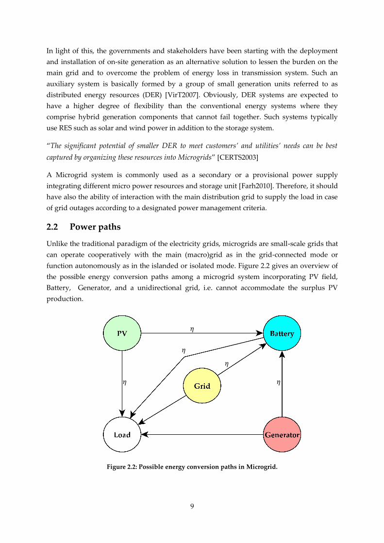
2.2 Power paths
Unlike the traditional paradigm of the electricity grids, microgrids are small-scale grids that
can operate cooperatively with the main (macro)grid as in the grid-connected mode or
function autonomously as in the islanded or isolated mode. Figure 2.2 gives an overview of
the possible energy conversion paths among a microgrid system incorporating PV field,
Battery, Generator, and a unidirectional grid, i.e. cannot accommodate the surplus PV
production.
𝜂
𝜂
𝜂 𝜂
Figure 2.2: Possible energy conversion paths in Microgrid.
𝜂

10
2.3 System Modeling
The considered microgrid system here is composed of a PV-array, a battery storage, and a
diesel generator set (GenSET), all together representing the proposed backup supply for the
essential loads, which all are connected to main grid through the point of common coupling
(PCC) as depicted in Figure 2.3
PV
Array
Battery
Storage
Diesel
GenSet
Main Grid
PCC
Critical
Loads
AC
DC
EMS
Legacy systemG(Grid/Diesel) New systemG(PV/Battery)
PD PB PPVPL
here:
unidirectional
power flow
Figure 2.3: General model of a PV-Battery-Diesel Microgrid system
Following is an abstract model of each system’s component and/or its main operational
constraints:
2.3.1 Load Demand
The load demand or profile represents the instantaneous power consumption of the load
and can be modeled by discrete values 𝑃𝐿(𝜏) over a fixed time horizon (e.g., a day),
where 𝜏 ∈ [𝑡0, 𝑡0 + 𝑇]. Obviously, the most important part of proposing an efficient
management strategy later on is to identify the consumption patterns and maintain power
supply even in blackouts, rather than to save energy. To this end, a method is required to
mockup a load profile for a relatively long period from available basic data. For the purpose
of testing control strategies, the load forecasting model should avoid complicated
configuration processes [PeBo2011]. Essentially, such a method is advantageous when a
comprehensive monitoring action is not possible either. Considering a load profile 𝑃𝐿(𝜏) is
available over a specific period which represents the basic data window. The consumption
pattern could be constant or assumed to have some slight changes over the original one (e.g.,
over the specified period), in which the load of the next window can be described as a term
of the main window but including a scaling factor and time delay, then the load profile for
the next day can be mathematically formulated as in Equ. (2.1):
𝑃𝐿′(𝜏) = 𝛼𝑖𝑃𝐿(𝜏 + 𝛽𝑖) (2.1)
11
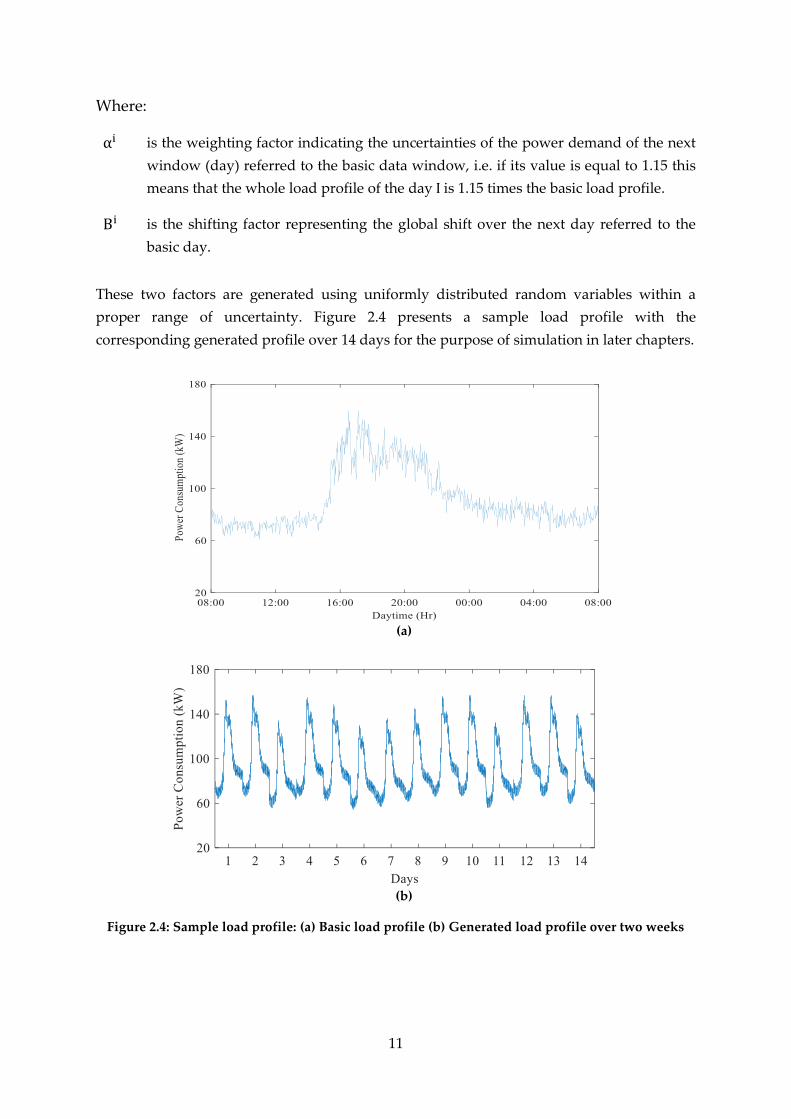
Where:
αi is the weighting factor indicating the uncertainties of the power demand of the next
window (day) referred to the basic data window, i.e. if its value is equal to 1.15 this
means that the whole load profile of the day I is 1.15 times the basic load profile.
Βi is the shifting factor representing the global shift over the next day referred to the
basic day.
These two factors are generated using uniformly distributed random variables within a
proper range of uncertainty. Figure 2.4 presents a sample load profile with the
corresponding generated profile over 14 days for the purpose of simulation in later chapters.
(a)
(b)
Figure 2.4: Sample load profile: (a) Basic load profile (b) Generated load profile over two weeks
12
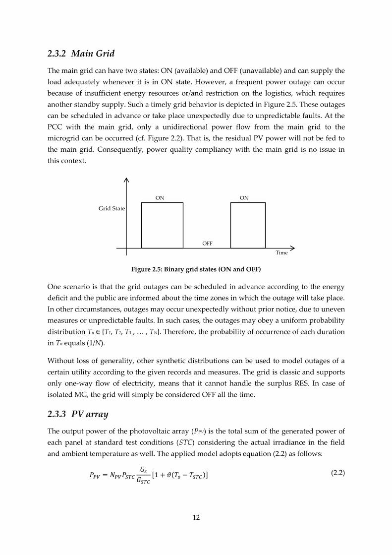
2.3.2 Main Grid
The main grid can have two states: ON (available) and OFF (unavailable) and can supply the
load adequately whenever it is in ON state. However, a frequent power outage can occur
because of insufficient energy resources or/and restriction on the logistics, which requires
another standby supply. Such a timely grid behavior is depicted in Figure 2.5. These outages
can be scheduled in advance or take place unexpectedly due to unpredictable faults. At the
PCC with the main grid, only a unidirectional power flow from the main grid to the
microgrid can be occurred (cf. Figure 2.2). That is, the residual PV power will not be fed to
the main grid. Consequently, power quality compliancy with the main grid is no issue in
this context.
Figure 2.5: Binary grid states (ON and OFF)
One scenario is that the grid outages can be scheduled in advance according to the energy
deficit and the public are informed about the time zones in which the outage will take place.
In other circumstances, outages may occur unexpectedly without prior notice, due to uneven
measures or unpredictable faults. In such cases, the outages may obey a uniform probability
distribution Tn ∈ {T1, T2, T3 , … , TN}. Therefore, the probability of occurrence of each duration
in Tn equals (1/N).
Without loss of generality, other synthetic distributions can be used to model outages of a
certain utility according to the given records and measures. The grid is classic and supports
only one-way flow of electricity, means that it cannot handle the surplus RES. In case of
isolated MG, the grid will simply be considered OFF all the time.
2.3.3 PV array
The output power of the photovoltaic array (PPV) is the total sum of the generated power of
each panel at standard test conditions (STC) considering the actual irradiance in the field
and ambient temperature as well. The applied model adopts equation (2.2) as follows:
𝑃𝑃𝑉 = 𝑁𝑃𝑉𝑃𝑆𝑇𝐶
𝐺𝑠
𝐺𝑆𝑇𝐶
[1 + 𝜗(𝑇𝑠 − 𝑇𝑆𝑇𝐶)] (2.2)
Grid State
Time
ON ON
OFF

13
where PPV, 𝑁𝑃𝑉, 𝑃𝑆𝑇𝐶, 𝐺𝑠, 𝐺𝑆𝑇𝐶, 𝜗, 𝑇𝑠, and 𝑇𝑆𝑇𝐶 are the output power from a the PV array at the
maximum power point (MPP), the total number of PV-modules that composed the solar
plant, the rated PV power at the MPP and STC, the irradiance level at the operating point
and at the STC, the power temperature coefficient at MPP, the panel temperature, and the
temperature at the STC, respectively.
The measure conditions at the STC are: GSTC = 1000 W/m2, TSTC = 25℃, and relative
atmospheric optical quality is AM1.5. Note that the output from the PV array are connected
directly to a dc-dc power converter which has inside a maximum power point tracking unit
(MPPT) to maximize power extraction under the different operational conditions.
The panel temperature 𝑇𝑠 is of course related to the ambient temperature 𝑇𝑎𝑚𝑏 and the
nominal operating cell temperature NOCT. It can be derived using equation (2.3) as follows:
𝑇𝑠 = 𝑇𝑎𝑚𝑏 +𝐺𝑠
800× (𝑁𝑂𝐶𝑇 − 20) (2.3)
Further details regarding the applied model can be found in [DjBw2013].
2.3.4 Battery Bank
The battery bank, is the most essential part of most microgrids. It is, therefore, necessary to
have a well-sized battery bank in order to ensure that the power supplied by RESs during
high generation periods will be available when the load requires it [MaY2014]. The strategy
of managing batteries can significantly impact the performance of the overall system. The
following condition is imposed to limit the power in/out flows of the battery:
|𝑃𝐵| ≤ 𝑃𝐵𝑚𝑎𝑥 (2.4)
where PB is the power thrown from or injected into the battery. It is positive at discharging
and negative at charging. It should not exceed a predefined limit in, 𝑃𝐵𝑚𝑎𝑥 all modes of
operation in order to slow down the degradation process [Jen2008]. Besides, another
variable that should be kept within a certain range is the state of charge (SoC). It can be
expressed as:
𝑆𝑜𝐶(𝜏) =𝐸𝐵𝑎𝑡(𝜏)
𝐶𝐵𝑎𝑡
(2.5)
𝑆𝑜𝐶𝑚𝑖𝑛 ≤ 𝑆𝑂𝐶 ≤ 𝑆𝑜𝐶𝑚𝑎𝑥 (2.6)
where EBat, CBat, 𝑆𝑜𝐶𝑚𝑖𝑛 and 𝑆𝑜𝐶max are the actual energy stored in the battery at time τ, the
total energy capacity of the battery, and the minimum and maximum allowed state of
charge of lead-acid batteries, respectively.
The SoC value at time (𝜏 + ∆) is determined by the SoC value at time τ and the battery power
during the time period. It can be expressed by the following equations:

14
𝐸𝐵𝑎𝑡(𝜏 + ∆) = 𝐸𝐵𝑎𝑡(𝜏) − 𝑃𝐵𝑎𝑡(𝜏) × ∆ (2.7)
𝑆𝑜𝐶(𝜏 + ∆) = 𝑆𝑜𝐶(𝜏) −𝑃𝐵𝑎𝑡(𝜏)
𝐶𝐵𝑎𝑡× ∆ (2.8)
The charging efficiency and discharging efficiency are both assumed to be 𝜂𝑏 = 95 %.
[PwrSnc].
Another important factor is the cumulative damage of the battery (CD), which can be
estimated by calculating the total cycles pass through the battery.
In particular, the number of cycles to failure (CFL) which defines the total lifetime of the
battery is the core factor to estimate CD. It depends mainly on how many cycles are passed
through the battery and how deep these cycles are, namely, the depth of discharge (DoD).
Basically, if a single cycle consumes (1/ CFL) of the whole life, then CD will become equal to
unity after CFL similar cycles and the battery will need to be replaced [VreP2011]. For
example, if the battery bank goes annually through K cycles, then the cumulative annual
damage is equal to:
C𝐷 = 𝐾(1/𝐶𝐹𝐿) (2.9)
This factor is also essential from an economical point of view to know the number of storage
unit replacement over the project period. Figure 2.6 shows the cycling behavior of a
commercial battery used for solar application under ideal operating conditions.
Figure 2.6: Cycle lifetime of a commercial OPzS battery as a function of DoC (at 20 ºC)
15
2.3.5 Diesel Generator
The diesel generator is the elementary component of the legacy system and acts as a backup
power supply in case of power outage or a complete disconnection from the utility grid. On
the other hand, it will assist the rest of microgrid’s components in case of insufficient power
production or weak charge in the storage system. The point of interest here is the driver or
the power provider which is the fuel. The relation between power production and fuel
consumption can be described using the fuel consumption chart of the diesel Generator
[MoP2014].
Mathematically, it can be modeled as a linear or quadratic function in accordance with the
given fuel consumption chart by the manufacturers [Dss2018]. The total fuel cost results
from the integration of the fuel consumption over the time. Equation (2.10), (2.11) and (2.12)
represent the generation limits, the total fuel consumption (Fc) in Liters and the fuel cost.
𝑃𝐺𝑒𝑛𝑚𝑖𝑛 ≤ 𝑃𝐺𝑒𝑛 ≤ 𝑃𝐺𝑒𝑛
𝑚𝑎𝑥 (2.10)
𝐹𝑐(𝑃) = ∑(𝑎𝑃2 + 𝑏𝑃 + 𝑐) × ∆ (2.11)
𝐹𝑢𝑒𝑙 𝐶𝑜𝑠𝑡 = 𝐷𝑐𝐹𝑐(𝑃) (2.12)
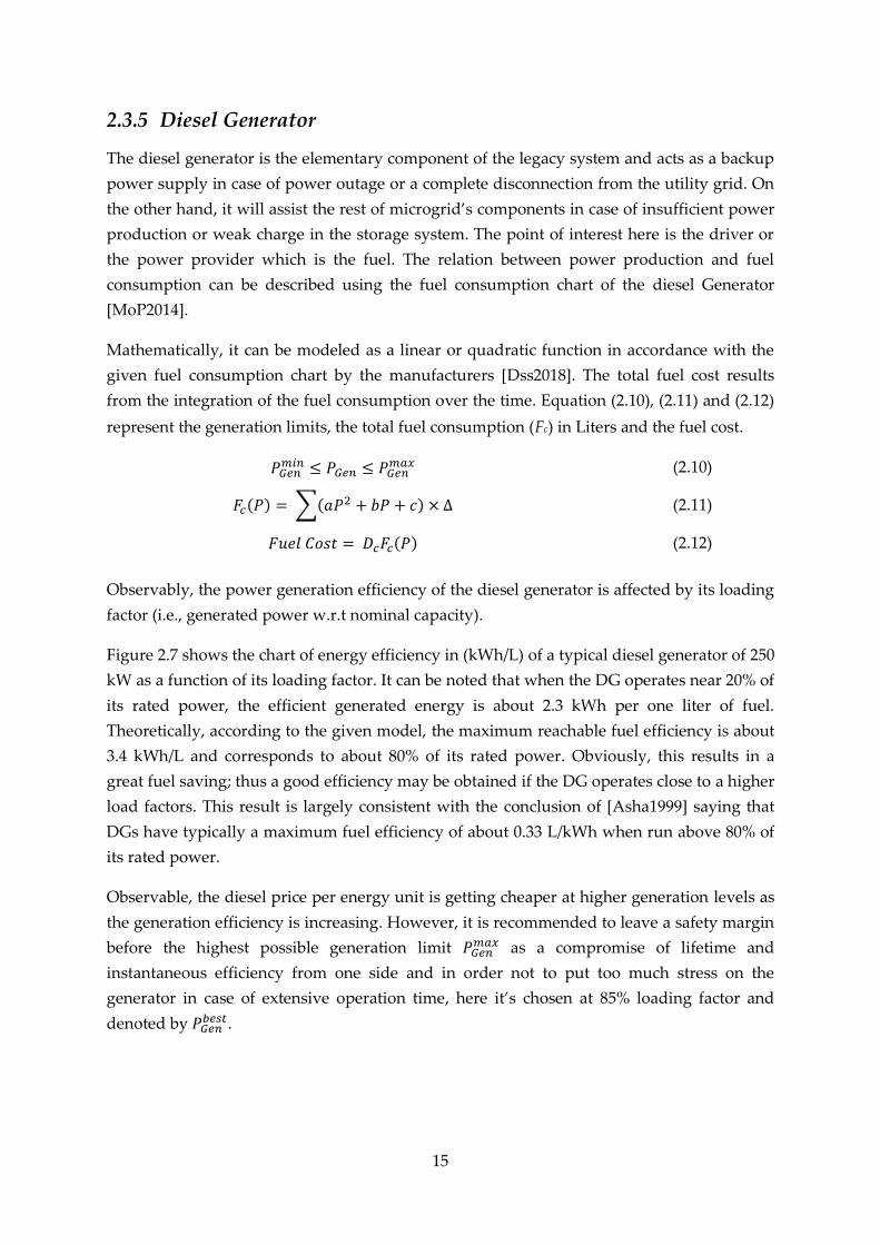
Observably, the power generation efficiency of the diesel generator is affected by its loading
factor (i.e., generated power w.r.t nominal capacity).
Figure 2.7 shows the chart of energy efficiency in (kWh/L) of a typical diesel generator of 250
kW as a function of its loading factor. It can be noted that when the DG operates near 20% of
its rated power, the efficient generated energy is about 2.3 kWh per one liter of fuel.
Theoretically, according to the given model, the maximum reachable fuel efficiency is about
3.4 kWh/L and corresponds to about 80% of its rated power. Obviously, this results in a
great fuel saving; thus a good efficiency may be obtained if the DG operates close to a higher
load factors. This result is largely consistent with the conclusion of [Asha1999] saying that
DGs have typically a maximum fuel efficiency of about 0.33 L/kWh when run above 80% of
its rated power.
Observable, the diesel price per energy unit is getting cheaper at higher generation levels as
the generation efficiency is increasing. However, it is recommended to leave a safety margin
before the highest possible generation limit 𝑃𝐺𝑒𝑛𝑚𝑎𝑥 as a compromise of lifetime and
instantaneous efficiency from one side and in order not to put too much stress on the
generator in case of extensive operation time, here it’s chosen at 85% loading factor and
denoted by 𝑃𝐺𝑒𝑛𝑏𝑒𝑠𝑡.
16
Figure 2.7: Diesel generator efficiency characteristics
2.3.6 Power Inverter:
A bi-directional power inverter is assumed to perform the needed power conversion
between AC and DC buses. The following equation describes an abstract model of the used
inverter:
𝑃𝑜𝑢𝑡 = 𝜂𝑐𝑃𝑖𝑛 (2.12)
where ηc is the efficiency of the power conversion.
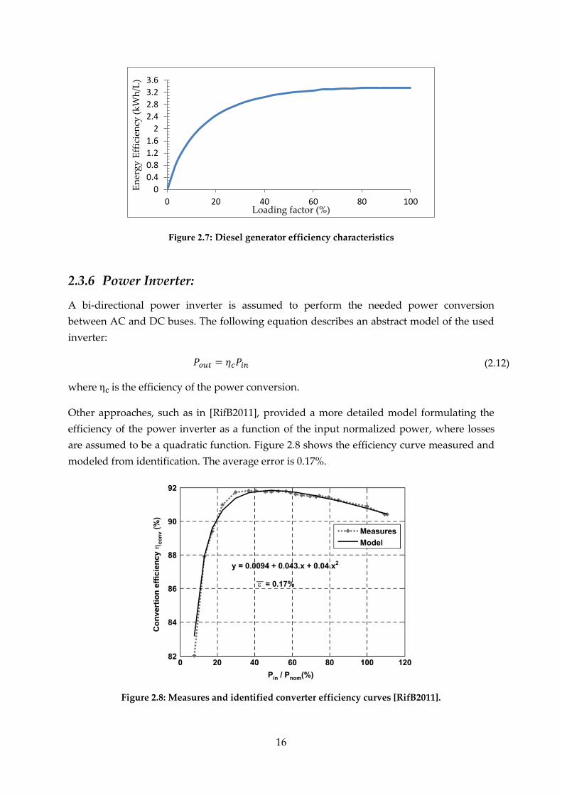
Other approaches, such as in [RifB2011], provided a more detailed model formulating the
efficiency of the power inverter as a function of the input normalized power, where losses
are assumed to be a quadratic function. Figure 2.8 shows the efficiency curve measured and
modeled from identification. The average error is 0.17%.
Figure 2.8: Measures and identified converter efficiency curves [RifB2011].
0
0.4
0.8
1.2
1.6
2
2.4
2.8
3.2
3.6
0 20 40 60 80 100
En
erg
y E
ffic
ien
cy (
kW
h/L
)
Loading factor (%)

17
2.4 Description of the Case Study
As introduced in the first chapter, this work is not oriented for a specific case only but can be
transformed to other environments according to the given requirements. Nevertheless, it is
not that simple to give a clear perception of the subject without elaborating by a real
example. For this reason, the presented case here will serve this purpose by incorporating
the aforementioned components in a one complete microgrid system and the discussion
later on will be on how to manage the operation of these components optimally without
violating the predefined operation constraints.
The considered case has been discussed in [MuKg2011], where a hybrid wind-diesel power
supply was proposed to cover a load profile of a hospital building in a more sustainable
way. The region is suffering from an energy crisis which adversely affects the power supply
of the hospital. A brief overview of the energy sector in that region will be presented firstly,
followed by a detailed description of the case under consideration and finally the current
applied energy management scheme of the existing backup power system there is going to
be presented.
2.4.1 Energy Sector in Gaza-Strip
Gaza-Strip is located in the South-West of Palestine. Its total area is estimated at 360 km2.
Gaza city is the major province in Gaza-Strip. It has one of the highest population densities
and overall growth rates in the world with its small total area of 45 square kilometers
[CiAwb]. According to the United Nation Office for the Coordination of Humanitarian
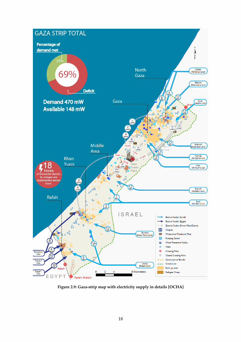
Affairs (OCHA) [OCHA2017]. Gaza-strip is supplied by electricity mainly through three
parties, namely: Gaza Power Plant (GPP), Egyptian lines (EL), and Israeli Electricity
Company (IEC). A detailed illustration of the power supply showing the distribution of the
these lines and the power demand and deficit is shown in Figure 2.9, according to the
situation in August 2014.
As depicted, Gaza-strip is suffering from an insufficient and irregular power supply.
According to the latest information by the Gaza Electricity Distribution Company (GEDCO),
the official body in charge of electricity supply in the Gaza Strip, power supply and deficit in
Gaza-Strip can be summarized by the diagram in Figure 2.10.
The impact of power outage in Gaza-Strip makes it difficult for GEDCO to schedule the
supply and distribute it in a proper way. Therefore, the authority in corporation with
GEDCO use to schedule or recirculate the supply between the different zones according to
the availability of power feeding lines. Depending on the status of GPP, the daily average
time of power-outage in all zones in Gaza-Strip may exceed twenty hours; including
hospitals and clinics. Further information about the energy sector in Gaza-Strip and the
origin of the problem up to August 2014 is covered in [WeS2009].
18
Figure 2.9: Gaza-strip map with electricity supply in details [OCHA]

19
(a)
(b) (c)
Figure 2.10: Gaza-strip electricity supply, [OCHA]
(a) Availability of electricity per month (average hours per day),
(b) Electricity supply per month (average megawatts), (c) Supply vs. demand (average megawatts)
2.4.2 Al-Shifa’ Hospital in Gaza-city
Al-Shifa' Hospital is the largest healthcare complex in Gaza-Strip. It has more than 600 beds
and serves more than 40 % of the population of Gaza-Strip [MuKg2011]. It consists of more
than 20 buildings and provides diagnostic, surgical care, emergency medical care, intensive
care, hospitality and labs. In addition to that it provides also general services such as
laundry, food preparation with delivery and personal cafeteria.

20
The hospital complex is supplied by medium voltage level (22 kV) from GEDCo through
two different feeding lines which are located in the northern and southern side of the
hospital. Each feeding line supplies two parallel MV-LV (22 kV/400 V – 0.85 MVA) three
phase transformers equipped into the two sub-stations as depicted in Figure 2.11
Figure 2.11: Al-Shifa’ Hospital’s power supplies [SkMoH]
Every sub-station is responsible of a group of buildings representing half of the hospital’s
total electric demand. Additionally, each sub-station is equipped with a group of different
capacities’ diesel generators (Standby Station N/S) that serve as an emergency power supply
system to cover the essential loads when the grid is unavailable.
Indeed, no other options are available to increase the capacity of any of the feeding lines in
order to meet all hospital’s demand every time sufficiently; where the grid cannot maintain
an acceptable voltage level at such high peak demand; otherwise, a huge modification need
to be done on the grid which means great investment cost and longtime of operations with
scarce income to both authority and distribution company.
The inevitable consequence of frequent and prolonged power outage, the administration of
the hospital with the consultant of engineering office stores diesel in special tanks inside the
hospital complex to operate the backup diesel generators when the grid is unavailable.
These tanks are prepared to store enough fuel to operate generators for one week of regular
power cut-off 12 hours/day in order to operate the essential loads normally. The authority in

21
Gaza-Strip gives the first priority to hospitals and healthcare facilities to supply them by
enough fuel to face the daily exacerbated challenge, but in the time of conflicts it becomes
impossible for authority to buy fuel directly.
Therefore, civil society organizations used to help as much as they can. 10 years ago, the
total rated power of each backup generator set at the two sub-stations was not more than
650 kVA, but the electricity crisis started sharply after 2006, when the local power plant was
partially destroyed [WiAlshifa]. Accordingly, the general administration of engineering and
maintenance there started to increase the capacity of generators to cover the increasing load
and to be on the safe side from the frequent power failure. In addition, during a prolonged
power outage, some normally non-essential services become essential, such as laundry,
catering or steam supply; these facilities cannot be stopped more than 16 hours in a daily
routine. Further clarification about how the engineering team there tries to beat the absence
of grid electricity every day is presented in the following subsection.
2.4.3 Existing Energy Management Experience
While load shedding of the hospitals in Gaza becomes a daily routine, all electric loads in the
hospital complex are subdivided into three categories according to the level of importance as
follows:
1. Essential loads (EL): These loads are essential to the life safety, critical patient care,
and the effective operation of the healthcare facility, and these loads are supplied by
the complete backup generators when the utility turns off to maintain the continuity
of the basic services in the hospital and keep the patient comfort at an acceptable
degree.
2. Very Important loads (VIL): This group of loads has a more sensitivity degree than
the previous group and cannot wait for longer time till the supply is back. The
included loads are automatically supplied by alternate power sources to supply any
of them at any interruption even if short period; usually those types of loads are
equipped with uninterruptable power supply (UPS) which can maintain good
supply during a certain period of time (maximum 10 minutes).
3. Non-essential loads (NEL): They express the remaining loads after subtracting EL
from all loads. They are not deemed essential to life safety, or the necessary
operation for the healthcare facility, such as offices’ air conditioning, incinerator,
general lighting, general lab equipment, service elevators, and patient care areas
which are not required to be backed up with an alternate source of power. However,
they must run sometimes in a weekly manner to keep the patient care at a good
situation.
In light of this information, the power system availability in Gaza’s hospitals can be divided
into three levels according to the available:
22
The green level: when grid is available and the backup diesel generators are ready to
operate without considerable concern about diesel transportation and logistics.
The yellow level: when the grid is unavailable but the backup diesel generators can
supply the essential load without fuel-logistic problems.
The red level: when the grid is unavailable and there is a scarcity in fuel supply due
to blocking in boarders or ports as occurred in conflicts.
The critical equipment such as in laboratories or clinics that are serious for a power outage
even of a short period of time (10 minutes maximum) are supplied by special (UPS) systems.
A set of UPS’s are distributed on some critical buildings such as: Dialysis, Neonatal Care,
Intensive Care Units, operatory rooms and some special diagnostic rooms.
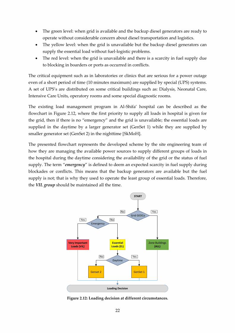
The existing load management program in Al-Shifa’ hospital can be described as the
flowchart in Figure 2.12, where the first priority to supply all loads in hospital is given for
the grid, then if there is no “emergency” and the grid is unavailable; the essential loads are
supplied in the daytime by a larger generator set (GenSet 1) while they are supplied by
smaller generator set (GenSet 2) in the nighttime [SkMoH].
The presented flowchart represents the developed scheme by the site engineering team of
how they are managing the available power sources to supply different groups of loads in
the hospital during the daytime considering the availability of the grid or the status of fuel
supply. The term “emergency” is defined to deem an expected scarcity in fuel supply during
blockades or conflicts. This means that the backup generators are available but the fuel
supply is not; that is why they used to operate the least group of essential loads. Therefore,
the VIL group should be maintained all the time.
START
Grid GEDCo
Zone Buildings (ALL)
Essential Loads (EL)
Daytime
GenSet 1 Genset 2
YesNo
YesNo
Loading Decision
Emergency
Very Important Loads (VIL)
NoYes
Figure 2.12: Loading decision at different circumstances.

23
This is done according to the experience of the operation engineers to save fuel and increase
the life time of the two generator sets; where they prefer to maintain the loading factor to a
certain generator round 85% and not less than 60 % of its rated capacity. In addition, it is
well known that the majority of loads will be online at the daytime, which means that
greater capacity is needed.
This is done according to the recommendation of several diesel generators’ manufacturers,
that the power generation limits of diesel generators correspond to the efficient fuel
consumption [Asha1999].
Unfortunately, the existing infrastructure does not support an efficient energy management
program as no monitoring-recording system has been installed yet; neither for the total
consumption of the buildings inside hospital nor for a certain group of critical facilities.
Moreover, it lacks break-down details of electrical energy consumption for different loads.
The availability of such a monitoring system can provide detailed load shapes of all different
facilities, which are of great interest for the following reasons:
Evaluating the consumption percentage of each load category according to the
corresponding criticality rank.
Auditing the total numbers of power failure or blackouts within a certain period of time,
(yearly/monthly/weekly or even daily based).
Following up the responding of backup system to the frequent power failures.
Forecasting the load of different categories according to their historical behavior.
Facilitating the prediction of the possible impact of the applied energy management
strategies.


25
3 Energy Management Strategies
Energy Management Strategies (EMSs) for Microgrids provide the key to ensure not only a
cost-effective but also an adaptable operation to the actual measurements. This chapter
highlights the major EMSs applied in this regard. It explores two approaches for power
routing in microgrids incorporating solar generation as an example of RES, battery energy
storage system (BESS), and a diesel generator, in addition to a unidirectional grid in case of
grid-connected system. The first approach is conventionally known as a rule-based EMS, and
the second one is a prediction-based which also known as an optimization-based EMS.
Furthermore, this chapter presents also a hybrid method for the purpose of adaptation with
the new measurements, which make use of both previous approaches to tackle the prediction
uncertainty efficiently. Finally, a brief demonstration of an advanced EMS is presented,
which is more resilient to the forecasting error and has the ability to realize the new
configuration in a shorter time.
3.1 Introduction
The continuous depletion of the fossil fuel and the global concerns about emission control
along with the needs for affordable power supply, all together bring out the hybrid
microgrids as promising alternative of the existing conventional power generation [Lr2002].
Such hybrid systems integrate a cluster of micro-sources, storage systems and loads, which
can operate as a single entity [MicaG2015]. However, to supply the load demand efficiently
in the most clean and economical way, the different incorporated energy resources must be
managed in an optimal manner [Lr2002].
Optimal EMS of a microgrid appears as a challenging problem because of the associated
challenges with the prediction. Namely, the fluctuating nature of the renewable energy
resources (RES) and the unpredictable part of the load demand. Therefore, a certain degree
of prediction is obviously needed to facilitate an optimal power coordination. In spite of
that, finding the optimal solution for this problem is actually challenging and is still an
active field of research because of the involved difficulties in solving such an optimization
problem. The major challenge is that, the associated continuous and discrete variables are to
be fixed. Fundamentally, defining the optimal switching time of each individual energy
source to supply the load and finding the associated power transactions among them.
Furthermore, a proper solution to this problem should also take care of maximizing the net
utilization of the installed RES and meanwhile minimizing the operational costs of other
conventional generation sources.
In the light of all these challenges, one can realize that a perfect EMS of a microgrid, such as
the considered one in this thesis, should first and foremost coordinate the generated power
of the conventional generation, the charging and discharging power of BESS, and the
generated power RES, in order to match the load demand according to certain optimization
criteria.
26
3.1.1 Related works
The literature is rich with the applied approaches for the purpose of power coordination in
microgrids. Because of its simplicity, the so-called rule-based EMS is mostly applied.
However, it cannot afford different objectives simultaneously. It is only oriented to cover the
requested load based on some logical assumptions made to compare and decide on the least
instantaneous price of available power from each generation element in the microgrid.
On the other hand, optimization-based approaches are mostly applied when a highly
accurate feeding of prediction is available of both generation and load [ref]. In this sense, the
most common technique used to solve this optimization problem is the linear programming
(LP) [HpWB2009]. However, it can only handle linearly formulated systems, which is not
always applied to such systems incorporate diesel generators of a quadratic function or
contain other elements with nonlinear functions. Other approaches used mixed-integer LP
(MILP) [PaGl2001], which are efficient to tackle the incorporated binary variables. Yet, the
main limitations towards applying such a general method to solve this problem is the need
for deploying the General Algebraic Modeling System (GAMS), or/and CPLEX which are
commercial solvers mostly used for such problems [ZaES2012]. Obviously, these methods
need further assistance to be able to reconfigure the microgrid and adapt the solution
continuously according to actual measurement [RiBP2011].
For this reason, a simple but effective method should be developed in order to tackle the
different operational constraints of the system and achieve the optimization requirements
more efficiently.
Modern control approaches such as Rolling or Receding Horizon (RH) make use of
optimization-based techniques and allow to tackle multiple objectives simultaneously
[OlMe2014], [BjTS2010]. These approaches are essentially identical to Model Predictive
Control (MPC) control where a rolling window is used for an optimization routine at each
iteration of the controller. The optimization portion can be formulated as a Mixed Integer
Linear Program (MILP) [HtLJ2011] or take on a nonlinear form [MfKh2007]. A comparison
of a similar heuristic algorithm and an MPC based EMS has been performed in [PaRG2014],
where the authors compare the total costs of an experimental microgrid in Athens, Greece.
These approaches can efficiently deal with economics, battery aging, controllable loads, and
many other important objectives concurrently. The reader is referred to [RaMS2013] for a
review of energy management techniques for microgrids.
In this chapter, these two approaches are going to be presented and discussed for active
power coordination for cost-efficient operation of a microgrid system consisting of PV, BESS,
diesel generator in addition to a unidirectional and frequently interrupting grid that cannot
buy or accept the surplus RES generation.
27
3.2 Rule-Based EMS
Rule-Based EMS is the simplest way to coordinate the power in microgrid. It represents in
fact a natural evolution of the binary decision process, where one has to choose between two
alternatives in order to take the present advantage of one of them, for instance might be
because of its affordable price or cleanness and eco-friendliness or even some other case-
specific conditions.
Suppose that a critical load is only supplied by a single power source, which can be called
the Main. As this is the only available power source, the cost of energy will be obviously
dominated by the power price of the Main. Besides, the natural response in case of Main’s
failure is to find another source to supply that load, which can be called Auxiliary. For
instance, if the price Auxiliary is lower than Main, then it will be of course more preferred to
supply the load. However, the tradeoff does not only exist between the price of both sources, but
also between the availability of each of them. Thus, an according to the rule of alternative cost,
the cost of NOT using the Auxiliary means the absence of the needed energy source.
Likewise, if we have multiple Auxiliaries with different availabilities and running costs,
then we have to rethink about some judging criteria, which can be specified by a group of
logical rules to assign the coming power requests in accordance with these predefined
preferences.
Simply, this approach is developed by assigning a priority to each power source according
to specific criterions. Usually, these criterions are purely economic but they might also
consider the fuel availability, or environmental issues. Fundamentally, the approach should
assign the power source that can supply the load sufficiently to take the responsibility over
other sources to supply the load at the moment. The remaining operational constraints, such
as generation limits of the generator or the grid capacity or the battery charge, must be of
course kept unviolated.
Principally, such a method dispatches energy based on the current measurements of the
available power and the state of charge of the battery and does not pay so much attention to
what will happen to the system afterwards. For instance, this method has been adopted in
[ZbcW2013] to coordinate the power in an off-grid system supplying a seawater desalination
project in the Dongfushan Island in China. It has been also explored in [RifB2009] to manage
a grid-connected system composed of PV generators, batteries storage, loads demand and a
bi-directional distribution grid.
Concerning the microgrid considered in this thesis, the developed Rule-Based EMS consists
of two concurrent checks, namely:
(1) the GRID-availability.
(2) the State-of-Charge check.

28
In all operation modes, the first priority is given to the PV supply and the rest of power
sources come to cover the deficit. The comprehensive explanation of these two checks and
their resulting decisions are given below:
1- Firstly, the utility grid is considered the Main here because of its availability and the
associated power price is commonly lower than the price of using other generators.
Thus, it is given the first priority after the solar generation to supply the load in case
of insufficient PV generation. However, as mentioned earlier, it cannot accommodate
the surplus by means of buying or feed-in tariff as other developed grid
infrastructures. Nevertheless, the grid in this operation mode is supposed to charge
the battery up to a certain limit SoCmax as long as its capacity allows.
2- Concurrently, the battery SoC is going to be checked whether it can supply the deficit
or not. In case of grid failure or power outage and insufficient PV too, the battery is
expected to have enough charge to supply the deficit. Subsequently, if the battery
SoC is lower than a predefined threshold, i.e. SoCmin, the request can then be directed
to the diesel generator as a last resort to cover the deficit.
Apparently, the Auxiliary elements are : (1) the utility grid, (2) the BESS, (3) the diesel
generator. And the priority is assigned to them respectively. However, once the BESS is
depleted to its lowest threshold, it cannot be discharged again without being recharged from
another power source. Hence, it acts occasionally as a load during the recharging process.
Therefore, in order to keep the battery SoC, it is allowed to charge the battery from the diesel
generator once requested to supply the deficit demand. Thus, the loading factor of the diesel
generator can be further increased and its associated fuel consumption efficiency will be
increased accordingly, cf. Ch. 2, diesel generator model.
Overall, the control strategy gives the priority of power supply to RES even if it is modest
comparable with diesel GenSet. Basically, the diesel GenSet operates in case of grid outage
and low SoC of the battery to supply the load demand and charge batteries (with excess
power) up to a certain point SoCmax according to the constraint in Equ. (2.6).
Note that two maximum threshold are chosen to stop the charging process: SoCstp1 is chosen
to stop the charging process from RES and SoCstp2 is chosen to stop the charging process
either from grid or from the diesel GenSet while it is running. Here, SoCstp2 is chosen lower
than SoCstp1 to maximize the usage of RES rather than depend too much on the grid or the
diesel GenSet.
In addition, the control strategy aims to operate the diesel GenSet in its most efficient range
by keeping the loading factor as high as possible instead of fluctuation according to load,
where the excess power is used to charge the battery as long as it does not violate the
charging constraints or the maximum permissible loading factor of the GenSet.

29
In order to avoid too fast (dis)charging of the batteries, another constraint is imposed to keep
the BESS healthy and prolong its lifetime, as in Equ. (2.4). Besides, high frequent changes in
the state of the diesel GenSet is prevented by allowing the generator to charge the battery
once operated up to the aforementioned threshold SoCstp2. The design parameters such as
battery (dis)charging limit 𝑃𝐵𝑚𝑎𝑥 and capacity of diesel GenSet 𝑃𝐷
𝑚𝑎𝑥 should be carefully
chosen according to the system behavior and characteristics. This issue is going to be
addressed in Chapter 5, Layout-Design.
A pseudocode of the developed rule-based EMS is presented in Figure 3.1

30
01: Declare state variables: 𝑃𝐿𝑖, 𝑃𝑃𝑉
𝑖 , 𝑃𝐵𝑖 , 𝑆𝑜𝐶𝑖, 𝐺𝑖, 𝑃𝐺
𝑖 , 𝑃𝐷𝑖 , 𝐹𝐷
𝑖
02: Declare GenSet coefficients: a, b, c
03: Declare parameters of operational constraints: 𝑆𝑜𝐶𝑠𝑡𝑝1, 𝑆𝑜𝐶𝑠𝑡𝑝2, 𝑆𝑜𝐶𝑚𝑖𝑛, 𝑃𝐵𝑚𝑎𝑥, 𝑃𝐷
𝑚𝑎𝑥
04: Declare time-slot, Gen. Flag, and efficiency: ∆T, 𝜂, 𝐷𝐺𝐹
05: Net deficit 𝑃𝐷𝑒𝑓𝑖 ∶= 𝑃𝐿
𝑖 − 𝜂 × 𝑃𝑃𝑉𝑖
06: IF (𝑃𝐷𝑒𝑓𝑖 ≤ 𝑃𝐿
𝑖) % surplus PV generation
07: 𝑃𝐷𝑖 ∶= 0
08: 𝑃𝐵𝑖 ∶= −𝑚𝑖𝑛{|𝑃𝐷𝑒𝑓
𝑖 |, 𝑃𝐵𝑚𝑎𝑥, (𝑆𝑜𝐶𝑠𝑡𝑝1 − 𝑆𝑜𝐶𝑖)}
09: 𝑃𝐺𝑖 ∶= 0
10: ELSE
11: IF(𝐺𝑖 == 1) % Grid is ON
12: 𝑃𝐷𝑖 ∶= 0
13: 𝑃𝐵𝑖 ∶= −𝑚𝑖𝑛{𝑃𝐵
𝑚𝑎𝑥, (𝑆𝑜𝐶𝑠𝑡𝑝2 − 𝑆𝑜𝐶𝑖) }
14: 𝑃𝐺𝑖 ∶= 𝑃𝐷𝑒𝑓
𝑖 − (𝑃𝐵
𝑖
𝜂)
15: ELSE % Grid is OFF
16: 𝑃𝐺𝑖 ∶= 0
17: IF ((𝑆𝑜𝐶𝑖 > (𝑆𝑜𝐶𝑚𝑖𝑛 + 𝑃𝐷𝑒𝑓𝑖 )) AND (𝐷𝐺𝐹 == 0))
18: 𝑃𝐵𝑖 ∶=
𝑃𝐷𝑒𝑓𝑖
𝜂% BESS supplies the deficit load
19: 𝑃𝐷𝑖 ∶= 0
20: ELSE
21: 𝑃𝐵𝑖 ∶= −𝑚𝑖𝑛 {(𝜂 × (𝑃𝐷
𝑚𝑎𝑥 − 𝑃𝐷𝑒𝑓𝑖 )) , 𝑃𝐵
𝑚𝑎𝑥, (𝑆𝑜𝐶𝑠𝑡𝑝2 − 𝑆𝑜𝐶𝑖) }
22: 𝑃𝐷𝑖 ∶= 𝑃𝐷𝑒𝑓
𝑖 − (𝑃𝐵
𝑖
𝜂) % Diesel supplies the deficit load and charge BESS
23: 𝐷𝐺𝐹 ∶= 1
24: IF (𝑆𝑜𝐶𝑖 ≥ 𝑆𝑜𝐶𝑠𝑡𝑝2)
25: 𝐷𝐺𝐹 ∶= 0 % Diesel is shut-down
26: END IF
27: END IF
28: END IF
29: END IF
30: SoCi+1 ∶= SoCi − (PB
i
∆T) % SoC update
31: 𝐹𝐷𝑖 ∶= (𝑎𝑃𝐷
𝑖 2+ 𝑏𝑃𝐷
𝑖 + 𝑐) × (1
∆T) % Incremental fuel consumption
Figure 3.1: A pseudocode of the developed rule-based EMS
31
3.3 Prediction-Based EMS
Unlike the former rule-based method, modern EMSs apply optimization techniques to
discover the operation schedule of the microgrid’s components while keeping several
predefined objectives together. However, the performance of such advanced solutions
depends strongly on the accuracy of the prediction. The goal is to determine how to route
the power from the different energy sources to supply the load in an efficient manner. In this
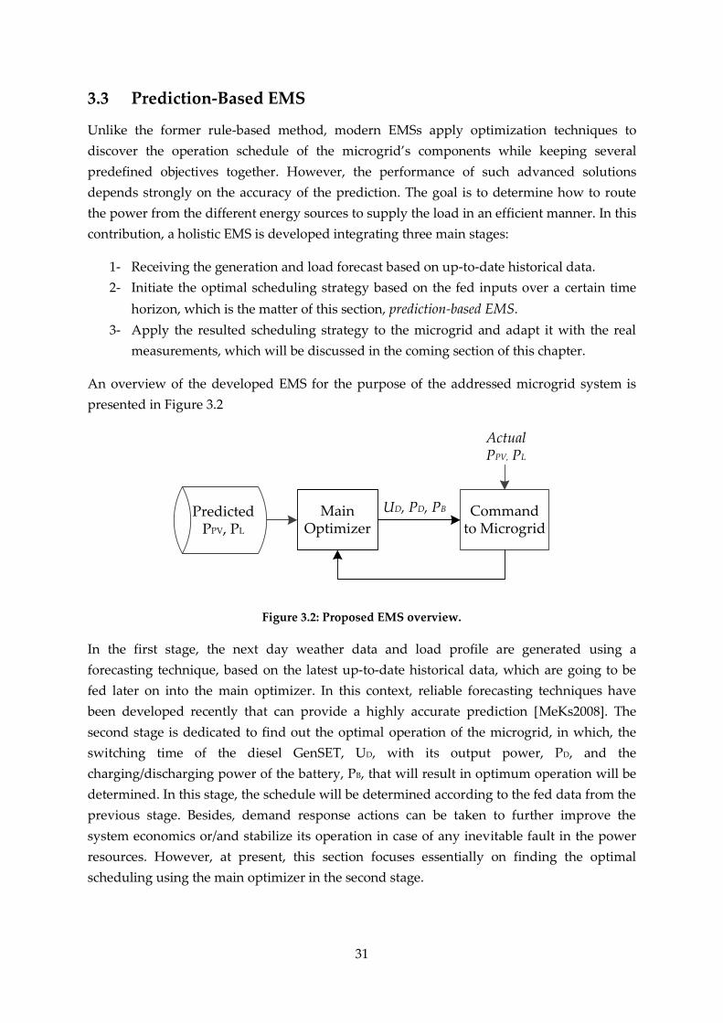
contribution, a holistic EMS is developed integrating three main stages:
1- Receiving the generation and load forecast based on up-to-date historical data.
2- Initiate the optimal scheduling strategy based on the fed inputs over a certain time
horizon, which is the matter of this section, prediction-based EMS.
3- Apply the resulted scheduling strategy to the microgrid and adapt it with the real
measurements, which will be discussed in the coming section of this chapter.
An overview of the developed EMS for the purpose of the addressed microgrid system is
presented in Figure 3.2
UD, PD, PBMainOptimizer
Predicted PPV, PL
Actual PPV, PL
Command to Microgrid
Figure 3.2: Proposed EMS overview.
In the first stage, the next day weather data and load profile are generated using a
forecasting technique, based on the latest up-to-date historical data, which are going to be
fed later on into the main optimizer. In this context, reliable forecasting techniques have
been developed recently that can provide a highly accurate prediction [MeKs2008]. The
second stage is dedicated to find out the optimal operation of the microgrid, in which, the
switching time of the diesel GenSET, UD, with its output power, PD, and the
charging/discharging power of the battery, PB, that will result in optimum operation will be
determined. In this stage, the schedule will be determined according to the fed data from the
previous stage. Besides, demand response actions can be taken to further improve the
system economics or/and stabilize its operation in case of any inevitable fault in the power
resources. However, at present, this section focuses essentially on finding the optimal
scheduling using the main optimizer in the second stage.
32
3.3.1 Optimization Framework
The addressed problem can be mathematically formulated as a multi-attribute optimization
problem that seeks to provide a minimum operating costs (𝑂𝐶) and maximum utilization
factor (𝑈𝐹) of a microgrid system, as well as guarantee that the operational constraints of the
battery, i.e., Equ. (2.4) to (2.8), and of the diesel generator, Equ. (2.10), are not violated.
Naturally, the power balance between generation and consumption must be achieved as in
equation (3.1).
0 LossLBDDPV PPPPUP (3.1)
Where PD is the generated power by diesel generator, PL is the instantaneous load demand,
and PLOSS is the total lost power, which are lost either in power conversion processes or not
utilized because of load satisfaction and battery charge saturation. UD denotes the status of
the diesel generator. The hat refers to the controllable variables, for example the power that
can be drawn from the diesel generator PD is controllable, however the solar generation PPV
is not directly controlled.
The value of OC is resulted mainly from the fuel consumption of the diesel GenSET and the
purchased energy from the grid in case of a grid-connected system. Further hidden costs can
be considered such as the aging of the battery and the total switching times of the diesel
GenSET which will complicate the problem. For this reason, the operational limits of the
battery and the generator are carefully chosen in accordance with the recommendation of
the manufacturers in order to prolong their lifespan as much as possible, e.g. Equ. (2.4), (2.8)
and (2.10).
By these definitions, the objective function can be then formulated as in equation (3.2) as
follows:
𝐽 = ∑ (𝑤1 ((𝑈𝐷(𝜏)) × 𝐹𝐶(𝑃𝐷(𝜏))) + 𝑤2(𝑈𝑃𝑉(𝜅𝜏)))
𝑇
𝜏=1
(3.2)
The value of 𝑈𝑃𝑉 is directly proportional with 𝑃𝐿𝑂𝑆𝑆, and represents the net unutilized RES
energy. It can be evaluated after applying the designated management strategy. Assuming
that a nonempty set 𝛫 ≠ ∅ of finite integer elements 𝑇 ∈ ∅ representing the total possible
operation strategies, where 𝐾 = {𝜅1, 𝜅2, 𝜅3, … , 𝜅𝑇}, and each individual operation strategy
will obviously produce a different value of 𝑈𝑃𝑉, where:
𝑈𝑃𝑉(𝜅𝜏) , 1 ≤ 𝜏 ≤ 𝑇
- 𝐹𝐶 is the fuel cost of the diesel generator corresponding to its generated power 𝑃𝐷
- 𝑈𝐷 is a binary value represents the state of operation of the diesel generator at time 𝜏
- 𝑤1works as a weighting factor, whereas 𝑤2works as a scaling and conversion factor
that converts the unutilized RES energy into a cost, e.g. ($).

33
Both factors are selected upon the design preferences and can be adapted according the
different operation scenarios to penalize the unutilized RES power and the usage of the
diesel generator.
Obviously, the value of the objective function, (Equ. 3.2) is controlled mainly by the output
power from the diesel GenSET, which is depending on the availability of the RES and
battery charge, that will delay the request time of the diesel GenSET.
Therefore, the problem involves finding the operation strategy κτ which can bring the
system to the optimal operation according to the aforementioned definitions. An operation
strategy κτ can be defined via three main control variables, which are: ��𝐷
1- The diesel GenSET status of operation ��𝐷
2- The diesel GenSET output power trajectory��𝐷 corresponds to the periods of ON
status.
3- Charging and discharging power trajectory��𝐵
The developed offline optimization solution for this problem will be addressed in the
following subsection.
3.3.2 Offline Optimization
The optimal schedule of the microgrid supply system will be explored in this work by
applying the dynamic programming (DP) to minimize the overall cost over the whole
prediction horizon (see Equ. 3.2). The idea of DP is to solve the multistage decision problem
by dividing it into sub-problems or several steps in order to examine all possible solutions at
each step and then combine these solutions in a way which leads to the best solution for the
given problem. It looks for the global optimal path rather than picking locally optimal
choices at each step which may result in a bad global solution. The advantage of the DP is
that it can handle constraints from all the natures (linear or not, differential or not, convex or
concave, etc.) and in meanwhile it does not need a specific mathematical solver to be
implemented [RiBP2011]. Obviously, in our case, the state of the system at each time-slot
depends on the previous state and the control variables, which can be replaced here, in the
context of DP, by the transitions.
In the discrete-time format, the system model can be expressed as:
𝑥(𝜏 + 1) = 𝑓(𝑥(𝜏), 𝑢(𝜏)) (3.3)
𝑥(𝜏) is the state vector of the system, and basically it includes the value of SoC which
controls the request of the diesel GenSET, and other variables which represent the rest
system dynamics such as: 𝑃𝑃𝑉, 𝑃𝐿.

34
𝑢(𝜏) is the control vector and should contain the abovementioned variables that are all
together controlling the selected operation strategy 𝜅𝜏. Both variables are defined explicitly
as follows:
𝑥(𝜏) = [𝑆𝑜𝐶 𝑃𝑃𝑉 𝑃𝐿] (3.4)
𝑢(𝜏) = [��𝐷 ��𝐷 ��𝐵] (3.5)
Conventionally, rule-based EMSs are applied to manage microgrid systems –as explained in
the previous section–, where the diesel generator is requested to supply the load when the
value of SoC goes beyond a certain limit SoCmin and turned off when there is sufficient RES
supply or the value of SoC goes over a higher threshold SoCmax, the proposed method here is
supposed to lead the system to the optimal trajectory by the assistance of prediction. These
former strategies are priority-based and do not benefit from the prediction. Therefore, these
so-called RB-based solutions, as developed also in [Hi++2016] and [RifB2009], may lead to a
higher cost in the future.
In contrast, the developed approach here using DP is a prediction-based and can explore the
optimal solution based on the fed forecast or planned load, so it can pick the optimal
strategy 𝜅𝜏 which will result in minimum objective value. Similarly, DP-based approaches
have been used in the literature for the same purpose considering different objectives
[RiBP2011], [BaLu2012] and [SobWu2012]. The main key for their implementation is to
quantize the value of the BESS storage and consider the possible SoC states’ transitions as
the determinant of the solution. However, the main limitation of these methods is the high
memory needs when the prediction horizon is long and discretized with a small time step
[RiBP2011].
To overcome this issue, the former DP approach is enhanced here by using the status of the
diesel GenSET ��𝐷 as the main coordinator to find the optimal strategy instead of using the
value of SoC. By this relaxation, the operation time of the diesel GenSET will be determined
firstly and then, the associated charging/discharging power trajectory of the battery can be
found based on the power balance constraint, (Equ. 3.1). This approach is clearly presented
by the graphical illustration of Figure 3.3.
To elaborate on the mechanism of the proposed approach, it is divided into two main stages,
the first stage is to choose one of the candidate strategy κτ that will be fed later on, in the
second stage, in order to explore its associated SoC trajectory. A candidate strategy κτ is a
binary-elements set representing the sequence of operation of the diesel GenSET, (as in the
upper part of the figure). It has the same length of the prediction horizon, (e.g, 𝑇 = 24 time-
slots).

35
Considering T is the total time-slots of the prediction horizon and there is two possible states
of the diesel generator which define the charging status of the battery, the resulting search
space is obviously 2T.
Compared with the previously applied method in [RiBP2011], where the DP is used to select
between N different levels of SoC at every time slot, the resulting number of iterations would
be NT. Therefore, the decomposition of the DP is proposed here as it enables the exploration
of a wide range of strategies in a much shorter time.
In our case, less than 1024 iterations were examined until they converged to a solution,
compared with 1024 if the SoC is quantized into ten levels. Notably, examining all strategies
will result in increasing burden of computational complexity. Therefore, the infeasible
solutions are firstly excluded, for instance, by eliminating the solutions which involve a
prolonged discharging time of the battery because this will ultimately lead to an excessive
discharging and of course passing the lower threshold SoCmin.
Figure 3.3: Relaxed DP searched-based EMS
3.3.3 Adaptation with the real measurements
Obviously, the resulting operation strategy from the previous stage, i.e. offline optimization, is
highly dependent on the fed forecast. On the other side, the microgrid is operated with
significant power fluctuating of the solar generation and the load profile as well. Thus, some
reconfigurability is apparently needed to tackle the real measurements which are, of course,
deviated somehow from the expected forecast, and this can be handled in the current stage.
ON ON
OFF
ON ON ON ON
T0 T1 T2 T3 T4 T5
SoC0
SoCmax
SoCmin
SoC = 100%
SoC = 0 %
OFF OFF OFF OFF OFF Die
sel
Sta
tes
Bat
tery
Sta
te o
f ch
arg
e

36
In this stage, the scheduling operator 𝜅𝜏 has the option to choose between the economic
operation mode which considers a perfect prediction, and stable operation which can
provide the sufficient supply to the actual net demand. Stable operation mode implies that,
the derived strategy can be varied in accordance with the actual measurements of the
generated PV power and load demand.
The selected strategy from the previous offline solution can be directly executed without
adaptation either in case of economical operation mode, where the operator has to keep the
derived schedule without changes, or whenever the prediction is totally perfect. However,
these two conditions are rarely achieved. For this reason, we propose an autonomous
adaptive operation strategy relying on the derived strategy in order to handle the expected
deficit caused by lack of PV generation or/and increased demand. A pseudocode of this
stage is illustrated in Figure 3.4
01: Declare state variables: 𝑃𝐿𝑖, 𝑃𝑃𝑉
𝑖 , 𝑆𝑜𝐶𝑖
02: Declare system parameters: 𝑆𝑜𝐶𝑚𝑖𝑛, 𝑆𝑜𝐶𝑚𝑎𝑥, 𝑃𝐷𝑚𝑖𝑛, 𝜂, ∆𝑇
03: Read a schedule 𝑘𝜏 = [𝑈𝐷 𝑃𝐷 𝑃𝐵]
04: Net deficit 𝑃𝐷𝑒𝑓𝑖 ∶= 𝑃𝐿
𝑖 − (𝜂𝑃𝑃𝑉𝑖 ) − (𝑈𝐷 × 𝑃𝐷) − 𝑑𝑖𝑠(𝑃𝐵)
05: Loop
06: Update 𝑃𝐷𝑒𝑓𝑖
07: IF ((𝑆𝑜𝐶𝑖 −𝑃𝐷𝑒𝑓
𝑖
𝜂) ≥ 𝑆𝑜𝐶𝑚𝑖𝑛)
08: 𝑃𝐷 keeps NO Change
09: BESS supplies
10: 𝑃𝐵 =𝑃𝐷𝑒𝑓
𝑖
𝜂
11: ELSE
12: 𝑃𝐷 = 𝑚𝑎𝑥(𝑃𝐷𝑚𝑖𝑛, 𝑃𝐷𝑒𝑓
𝑖 )
13: 𝑃𝐵 = 𝜂 × (𝑃𝐷 − 𝑃𝐷𝑒𝑓𝑖 )
14: END IF
15: Update SoC := 𝑆𝑜𝐶𝑖+1 ∶= 𝑆𝑜𝐶𝑖 − (𝑃𝐵
𝑖
∆𝑇)
16: END Loop
Figure 3.4: A pseudocode of the adaptation stage, 3rd Block of EMS.
Firstly, the system parameters are identified in order not to violate the operation constrains
and to keep the generator operated at a reasonable loading factor. The deterministic
operation strategy is gathered from the previous stage of EMS and then the current
measurements are fed. Consequently, a supplementary decision is taken to supply the
deficit load either from BESS or diesel generator. The key determinant here is the reserve
SoC and the deficit value. Obviously, the battery is preferred to cover the deficit if it has
enough charge in order to operate the generator for short time.

37
However, if the diesel generator is the remaining choice because of insufficient SoC, it
should not be operated at a lower loading factor than 𝑃𝐷𝑚𝑖𝑛.
3.4 Stochastic Optimization EMS
The optimization algorithm employs a Genetic Algorithm (GA), which is one of the
metaheuristic stochastic optimization techniques that can provide a solution to an
optimization problem with less computational effort than iterative ones [HiFr2018a].
Examining all strategies will result in increasing burden of computational complexity. The
search space of the problem is obviously very large. Considering two possible status of the
diesel generator at each time slot, the number of resulting iterations would reach (2𝑁) of
iterations, each requiring k time-units to consider constraints, Equ. (2.4) to (2.8), (2.10), and
evaluate Equ. (3.1), and (3.2). If all possible combinations will be checked; the resulting time-
units will be (𝑇 × 2N) and it is, of course, exponentially increased w.r.t chosen time horizon.
Therefore, the GA is chosen as it enables the exploration of a wide range of allotted elements
in a much shorter time. In our case, less than 60 generations were examined until they
converged to the final solution (here: just a few seconds of computation time instead of
minutes using the deterministic approach).
To improve the time performance of the algorithm, the infeasible solutions are firstly
excluded by eliminating the solutions which include a prolonged discharging time of the
battery because this will ultimately lead to an excessive discharging of the BESS and of
course passing the lower threshold SoCmin. The maximum durable discharging time, in
hours, is calculated to exclude any operation strategy that will eventually lead to a wider
discharging period. It is assumed that the battery bank is fully charged up the nominal
capacity, e.g. 𝐸𝐵𝑚𝑎𝑥(kWh), and the load is the average net deficit that should be met either by
the battery or the generator. This is presented by the equation 3.6
𝛭 = ⌊𝐸𝐵
𝑚𝑎𝑥
𝑎𝑣𝑔(𝑃𝐷𝑒𝑓)⌋ (3.6)
Where M is the maximum nonstop discharging time, 𝐸𝐵𝑚𝑎𝑥 is the nominal capacity of the
battery bank in (kWh), and 𝑎𝑣𝑔(𝑃𝐷𝑒𝑓) is the average net deficit, in (kW).
The default settings of MATLAB-based GAs are applied to conduct the simulation. A
population of chromosomes is randomly initialized (i.e., 200) in accordance to the possible
number of solutions. The algorithm is supposed to be terminated when the stipulated
number of generations (i.e., 500) is reached or when the magnitude in the change in fitness
value does not vary more than a tolerance limit (i.e., 10-10) for several subsequent generations
(i.e., 50). A pseudo-code of the developed GA framework is depicted in Figure 3.5. Each
selected candidate 𝜅𝜏 will be examined at each generation to find out the best fitness
function (Equ. 3.2).
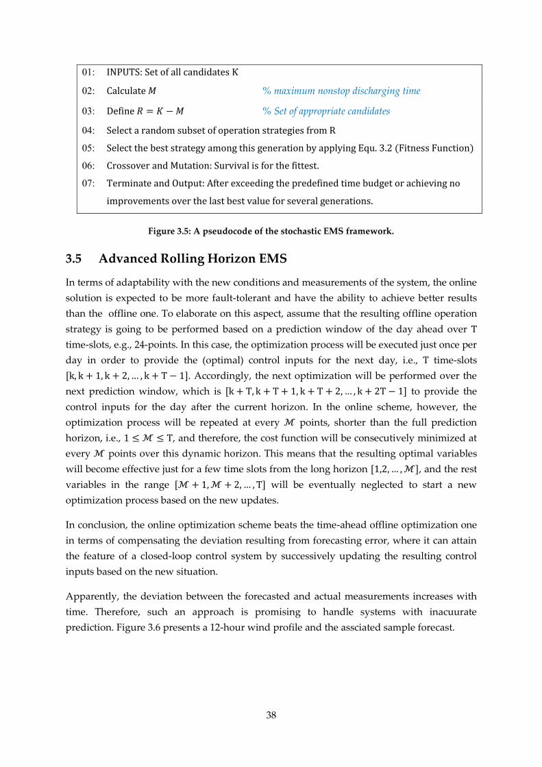
38
01: INPUTS: Set of all candidates Ƙ
02: Calculate 𝛭 % maximum nonstop discharging time
03: Define 𝑅 = 𝐾 − 𝛭 % Set of appropriate candidates
04: Select a random subset of operation strategies from R
05: Select the best strategy among this generation by applying Equ. 3.2 (Fitness Function)
06: Crossover and Mutation: Survival is for the fittest.
07: Terminate and Output: After exceeding the predefined time budget or achieving no
improvements over the last best value for several generations.
Figure 3.5: A pseudocode of the stochastic EMS framework.
3.5 Advanced Rolling Horizon EMS
In terms of adaptability with the new conditions and measurements of the system, the online
solution is expected to be more fault-tolerant and have the ability to achieve better results
than the offline one. To elaborate on this aspect, assume that the resulting offline operation
strategy is going to be performed based on a prediction window of the day ahead over T
time-slots, e.g., 24-points. In this case, the optimization process will be executed just once per
day in order to provide the (optimal) control inputs for the next day, i.e., T time-slots
[k, k + 1, k + 2, … , k + T − 1]. Accordingly, the next optimization will be performed over the
next prediction window, which is [k + T, k + T + 1, k + T + 2, … , k + 2T − 1] to provide the
control inputs for the day after the current horizon. In the online scheme, however, the
optimization process will be repeated at every ℳ points, shorter than the full prediction
horizon, i.e., 1 ≤ ℳ ≤ T, and therefore, the cost function will be consecutively minimized at
every ℳ points over this dynamic horizon. This means that the resulting optimal variables
will become effective just for a few time slots from the long horizon [1,2, … , ℳ], and the rest
variables in the range [ℳ + 1, ℳ + 2, … , T] will be eventually neglected to start a new
optimization process based on the new updates.
In conclusion, the online optimization scheme beats the time-ahead offline optimization one
in terms of compensating the deviation resulting from forecasting error, where it can attain
the feature of a closed-loop control system by successively updating the resulting control
inputs based on the new situation.
Apparently, the deviation between the forecasted and actual measurements increases with
time. Therefore, such an approach is promising to handle systems with inacuurate
prediction. Figure 3.6 presents a 12-hour wind profile and the assciated sample forecast.

39
Figure 3.6: Sample forecast generated for a 12-Hr wind profile [SuGD2012]
3.6 Simulation Results
PV-BSS microgrid system used to supply the critical loads in an outpatient clinic in Gaza city
is chosen to check the aforementioned approaches except the last one, i.e. Rolling Horizon.
The system has been under developing over the past years to lessen the consequences of the
severe power outages that Gaza-strip undergoes. The hourly-average prediction and the
associated actual values of both solar generation and load demand of a single day are shown
below in Figure 3.7. The simulation is firstly performed using the priority-based EMS,
followed by the offline-optimization solution and finally the uncertainty is applied to check
compare with the adaptation strategy as well.
The former approach, i.e., priority-based EMS, is taken as a baseline to compare the rest
approaches with it and highlight the cost savings. Additionally, the net share of PV in is
another important key performance factor indicates the real benefit of deploying the RES in
the system and gives a better realization of the presented outcomes. It can be described by
two values, the penetration level (PL) and the utilization factor (UF) which both are defined
in equations (3.7) and (3.8) as follows:
%production RESTotal
RESby suppliedenergyNetUF 100 (3.7)
%demandenergyTotal
RESby suppliedenergyNetPL 100 (3.8)
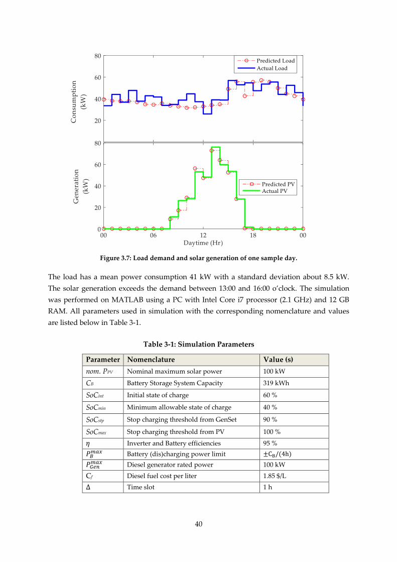
40
Figure 3.7: Load demand and solar generation of one sample day.
The load has a mean power consumption 41 kW with a standard deviation about 8.5 kW.
The solar generation exceeds the demand between 13:00 and 16:00 o’clock. The simulation
was performed on MATLAB using a PC with Intel Core i7 processor (2.1 GHz) and 12 GB
RAM. All parameters used in simulation with the corresponding nomenclature and values
are listed below in Table 3-1.
Table 3-1: Simulation Parameters
Parameter Nomenclature Value (s)
nom. PPV Nominal maximum solar power 100 kW
CB Battery Storage System Capacity 319 kWh
SoCint Initial state of charge 60 %
SoCmin Minimum allowable state of charge 40 %
SoCstp Stop charging threshold from GenSet 90 %
SoCmax Stop charging threshold from PV 100 %
𝜂 Inverter and Battery efficiencies 95 %
𝑃𝐵𝑚𝑎𝑥 Battery (dis)charging power limit ±CB/(4h)
𝑃𝐺𝑒𝑛𝑚𝑎𝑥 Diesel generator rated power 100 kW
Cf Diesel fuel cost per liter 1.85 $/L
∆ Time slot 1 h
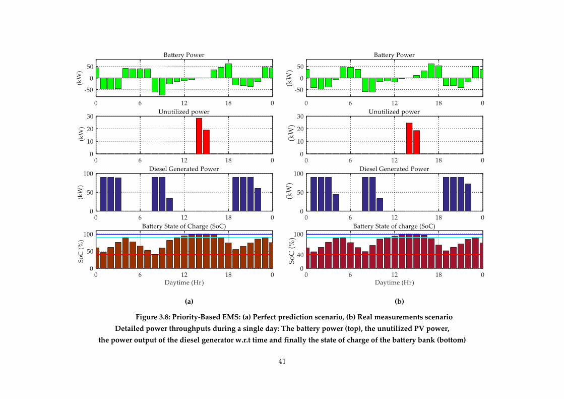
(a) (b)
Figure 3.8: Priority-Based EMS: (a) Perfect prediction scenario, (b) Real measurements scenario
Detailed power throughputs during a single day: The battery power (top), the unutilized PV power,
the power output of the diesel generator w.r.t time and finally the state of charge of the battery bank (bottom)
41
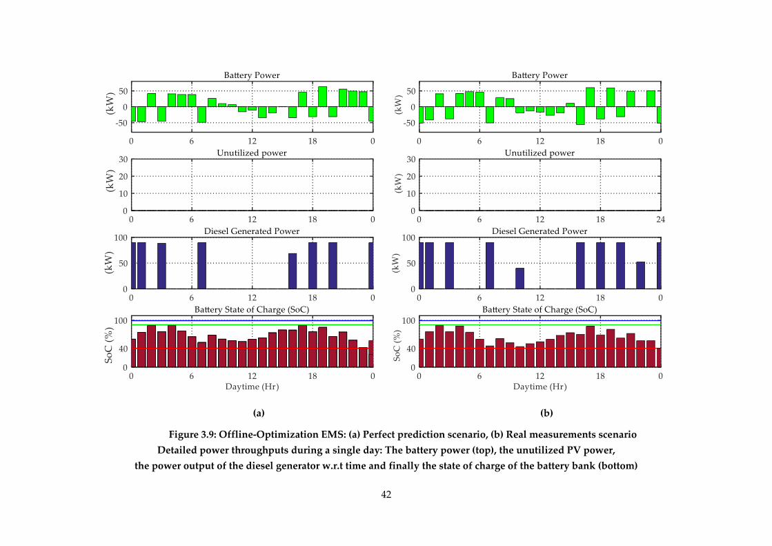
42
(a) (b)
Figure 3.9: Offline-Optimization EMS: (a) Perfect prediction scenario, (b) Real measurements scenario
Detailed power throughputs during a single day: The battery power (top), the unutilized PV power,
the power output of the diesel generator w.r.t time and finally the state of charge of the battery bank (bottom)
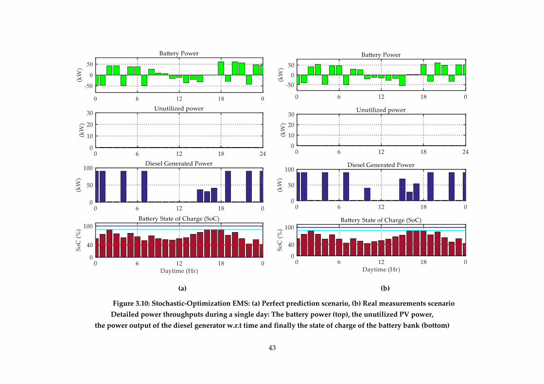
43
(a) (b)
Figure 3.10: Stochastic-Optimization EMS: (a) Perfect prediction scenario, (b) Real measurements scenario
Detailed power throughputs during a single day: The battery power (top), the unutilized PV power,
the power output of the diesel generator w.r.t time and finally the state of charge of the battery bank (bottom)

Figure 3.8 presents the results of the former priority-based EMS considering the predicted
profiles as well as the real measurements. It is noted that the results in both scenarios are
similar to a large extent. However, due to the energy difference between the predicted and
the real measurements, the unutilized PV energy considering the real scenario is slightly
less, namely 43.12 kWh instead of 47.42. In spite of that, this amount of energy was lost
during the middle of the day, at 14:00 and 15:00. Observably, at that time, the BESS was fully
charged and could not accommodate the surplus PV generation. So, the battery SoC at that
time went beyond the SoCstp2 threshold and therefore, one can recognize that the oscillation
range of the associated SoC takes the interval from SoCmin to SoCstp1. Too, in spite of the high
demand at midday, it is observed that the battery was exposed to a less stress at noon than
at the two ends of the day. Visibly, this can be interpreted by the higher PV production. One
additional difference is the operation time of the diesel generator, where it was operated for
another hour in the case of real measurements.
Figure 3.9 and 3.10 present the simulation results of the offline-optimization and stochastic-
optimization EMS respectively. The simulation considered both scenarios too, the predicted
and the real measurements as well. These methods are based on optimization and therefore
once can recognize that the unutilized PV energy are zero, which means that only the power
conversion losses exist in that case rather than the conventional method which did not
benefit from much more energy in addition to the power conversion loss and thus, the
battery in the prediction-based EMS is expected to have enough vacancy to absorb the
emergence of surplus renewable power during the noon, i.e., between 12:00 to 17:00.
However, in both cases, the operation time of the diesel generator considering the real
measurements scenario is longer than the counterpart perfect prediction scenario. For
instance, the operation time was eight hours considering the perfect prediction by using the
offline-optimization method, where this method represent the best case scenario, as shown
in Figure 3.9(a). On the other side, the generator was subject to operate at least 10 hours
using the stochastic optimization solution, as shown in Figure 3.10(a). However, the
increment in case of real measurements was two hours in case of the offline-optimization,
and only one-hour in case of the stochastic solution.
Compared to the priority-based EMS method, as in Figure 3.8, it is observed that the
oscillation range of the battery SoC was less by using the prediction-based EMS, as in Figure
3.9 and 3.10. Besides, the battery reached the upper threshold SoCstp2 but did not go beyond
it at the evening time, when the generator was in operation.
From these figures, one can notice how the operation of both diesel generator and BESS are
affected. However, the operation in the adaptive-mode was more stable because it could
handle the inaccurate prediction. Therefore, there will be no need for load shedding when
considering the adaptation algorithm because of the ability of handling the prediction errors.
44

45
The fuel consumption using the prediction-based approaches is still less than the
consumption using the conventional priority-based method. However, in the adaptive
mode, the fuel consumption is a bit greater than its counterpart in the perfect prediction
case, and this is expected because the deficit difference between the two cases is about 59
kWh, where the total actual PV generation is 9 kWh lower than the predicted generation and
the consumption is about 50 kWh greater than the predicted load. It is expected therefore,
that this gap will be covered using the conventional generation. Obviously, the SoC of the
BESS in both cases is softly ranging between SoCmin and SoCmax. In addition to that, a
sufficient margin is kept up to the fully charged level, 100% SoC, in order to be able to
accommodate any unexpected raise in solar generation.

46
Table 3-2: Simulation results of EMS using the prediction-data
Parameter RB-EMS Deterministic
Prediction-Based
Stochastic
Prediction-Based
Total demand (kWh) 980.54
Total gross PV energy (kWh) 386.04
Net utilized PV energy (kWh) 304.76 347.43 347.43
Unutilized PV (kWh) 47.41 0 0
Power conversion loss (kWh) 33.87 38.61 38.61
Total PV energy loss (kWh) 81.28 38.61 38.61
Utilization Factor (UF) 78.95 % 89.99 % 89.99 %
Penetration Level (PL) 31.08 % 35.43 % 35.43 %
Total fuel consumption (Liter) 235.26 173.92 191.25
Total fuel costs ($) 435.23 321.75 353.81
Operation Hours (Hr) 10 7 9
Table 3-3: Simulation results of EMS using the real-data
Parameter RB-EMS Deterministic
Prediction-Based
Stochastic
Prediction-Based
Total demand (kWh) 1040.94
Total gross PV energy (kWh) 377.02
Net utilized PV energy (kWh) 300.51 339.32 339.32
Unutilized PV (kWh) 43.11 0 0
Power conversion loss (kWh) 33.40 37.70 37.70
Total PV energy loss (kWh) 76.51 37.70 37.70
Utilization Factor (UF) 79.70 % 89.99 % 89.99 %
Penetration Level (PL) 28.86 % 32.59 % 32.59 %
Total fuel consumption (Liter) 252.76 209.4 215.36
Total fuel costs ($) 467.61 387.4 398.42
Operation Hours (Hr) 11 9 10


48
4 Demand Side Management
One important key feature of the modern power system paradigm is to have some
controllability over the load demand rather than following the ever growing consumption by
increasing the generation. Demand Side Management as a concept can be simply defined as
any actions taken to influence the consumption side in order to be operated in an energy-
efficient way. This does not necessarily imply that the consumption must be minimized, but
optimized. One drastic solution could be getting completely rid of the unnecessary load.
Another intermediate scheme is to adjust the consumption time to take place during the low-
price generation time rather than supply-once-plugged scheme. However, these solutions
could lead to uncomfortable operation conditions if the users’ preferences are not carefully
considered. Therefore, a balance should be achieved between the low-price generation time
and the operational constraints of these loads in order to achieve the goal of optimization.
This chapter presents a Forecast-Driven Power Planning Approach for Microgrids
Incorporating Smart Loads.
4.1 Introduction
Until recently, various approaches have been proposed and applied to coordinate the
generation sources in order to meet the varying demand while keeping the electricity cost at
optimal levels [Zhu2009]. However, due to ever increasing demand and motivated by the
affordable prices of the renewable-energy based systems, a growing desire exists to control
or optimize the demand growth in order to facilitate the integration of RES into domestic
and industrial sectors. Yet, the fluctuating nature and intermittency of the RES are the still
forming a barrier against entirely relying on them as a main power provider or even
increasing their penetration level in generation side. In spite of that, this obstacle can be
overcome by using a proper energy storage to stabilize the operation and compensate the
shortage. This solution is not always affordable, especially in standalone and remote
systems, or in buildings subject to severe power outages, where the fluctuating supply
cannot be matched by a greater energy storage on all occasions. Otherwise, this will simply
add cost and complexity to the system.
A potential alternative solution will be influencing the load demand, totally or partially, in
order to lower the need for a larger energy reserve [PaD2011]. A good scheduling of some
shiftable loads can improve the reliability of power delivery for customers during
(macro)grid blackouts or emergency islanded operation. Once the system is integrated with
some smart loads, that can be scheduled in advance, an efficient algorithm could be
developed to reallocate these loads in another time, in which, the total energy cost can be
minimized and the utilization of RES can be maximized as well.
The need for some controllability over load is not only to assist in accommodating more RES
into different power systems around the world, but also there is an important and persistent
need to develop and apply such a solution in countries which have weak power systems or
suffer from continuously interruption of the utility grid.

49
Especially in developing countries, a large number of buildings including healthcare
facilities, schools and small businesses are suffering from a serious lack of a continuous and
stable power supply. This issue has forced the decision makers and the stakeholders to look
for some temporary solutions that can alleviate the drawbacks of such a problem.
Conventionally, diesel generators are used to cover the ever increasing demand during the
outage time, which are costly and environmentally unfriendly too. The reason behind not
using such a forecast-driven approach previously, is the need for efficient forecasting tools
that can predict the upcoming load and production accurately.
4.1.1 Related works
A huge work has been done in the context of load scheduling. A heuristic algorithm to
schedule a group of smart appliances in a smart building subject to a real-time pricing has
been proposed in [LeBa2013]. Another work has been conducted on a smart building
environment but using a set of household appliances that allow for a limited interruption
time [CaDF2015]. A heuristic-based load shifting optimization approach has been proposed
in [LoSh2012], where three adjacent power networks have been chosen to carry out the
study. Another load scheduling algorithm based on game theory has been proposed in
[MoW2010]. The main objective was to optimize the energy costs by reducing the aggregate
peak-to-average ratio of the total energy demand, while respecting the privacy of the
customers.
Considering the previously listed literature review and the other ongoing work in this
domain; e.g. [HabK2016], [MaR2016], [OBr2016], and [HiFr2018d], it has been realized that
the number of studies that have discussed the problem of scheduling dynamic non-
preemptive loads from the perspective of standalone microgrids are not much.
Two reasons maybe behind that, which are: the complexity of solving such a load scheduling
problem, which is similar to NP-hard problems [BaGo2004], and the difficulties involved in
modelling such continuously-operating loads with a non-fixed power consumption.
4.1.2 Scope of work
As introduced, this chapter takes care of the load scheduling in smart building as an
important function of the tertiary level in controlling microgrids. Thus, the scope of the
work does not include the voltage stability or power quality at the point of common
coupling (PCC). However, it tackles the uppermost control level, which has the longest
discrete time steps; e.g. ranging from intra-hours to intra-days. To this end, this work offers
a proactive scheduling plan for the smart loads which announce their desired operation
pattern or the associated consumption profiles in advance; e.g. a day ahead. In other words,
the proposed algorithm will attempt to reallocate the aggregated loads to closely follow the
low-price available power; e.g. from utility grid or local RES generation.
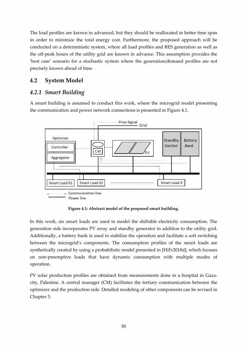
50
The load profiles are known in advanced, but they should be reallocated in better time span
in order to minimize the total energy cost. Furthermore, the proposed approach will be
conducted on a deterministic system, where all load profiles and RES generation as well as
the off-peak hours of the utility grid are known in advance. This assumption provides the
‘best case’ scenario for a stochastic system where the generation/demand profiles are not
precisely known ahead of time.
4.2 System Model
4.2.1 Smart Building
A smart building is assumed to conduct this work, where the microgrid model presenting
the communication and power network connections is presented in Figure 4.1.
Figure 4.1: Abstract model of the proposed smart building.
In this work, six smart loads are used to model the shiftable electricity consumption. The
generation side incorporates PV array and standby generator in addition to the utility grid.
Additionally, a battery bank is used to stabilize the operation and facilitate a soft switching
between the microgrid’s components. The consumption profiles of the smart loads are
synthetically created by using a probabilistic model presented in [HiFr2018d], which focuses
on non-preemptive loads that have dynamic consumption with multiple modes of
operation.
PV solar production profiles are obtained from measurements done in a hospital in Gaza-
city, Palestine. A central manager (CM) facilitates the tertiary communication between the
optimizer and the production side. Detailed modeling of other components can be revised in
Chapter 3.
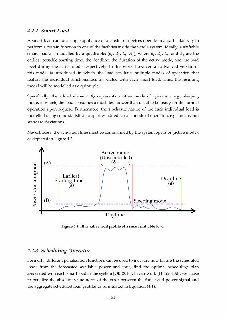
51
4.2.2 Smart Load
A smart load can be a single appliance or a cluster of devices operate in a particular way to
perform a certain function in one of the facilities inside the whole system. Ideally, a shiftable
smart load ℓ is modelled by a quadruple: (𝑒ℓ, 𝑑ℓ, 𝐿ℓ, 𝐴ℓ), where 𝑒ℓ, 𝑑ℓ, 𝐿ℓ, and 𝐴ℓ are the
earliest possible starting time, the deadline, the duration of the active mode, and the load
level during the active mode respectively. In this work, however, an advanced version of
this model is introduced, in which, the load can have multiple modes of operation that
feature the individual functionalities associated with each smart load. Thus, the resulting
model will be modelled as a quintuple.
Specifically, the added element 𝐴ℓ represents another mode of operation, e.g., sleeping
mode, in which, the load consumes a much less power than usual to be ready for the normal
operation upon request. Furthermore, the stochastic nature of the each individual load is
modelled using some statistical properties added to each mode of operation, e.g., means and
standard deviations.
Nevertheless, the activation time must be commanded by the system operator (active mode),
as depicted in Figure 4.2.
Active mode(Unscheduled)
Sleeping mode
DeadlineEarliest
Starting-time-
Po
wer
Co
nsu
mp
tio
n
Daytime
(e) (d)
(L)(A)
(B)
Figure 4.2: Illustrative load profile of a smart shiftable load.
4.2.3 Scheduling Operator
Formerly, different penalization functions can be used to measure how far are the scheduled
loads from the forecasted available power and thus, find the optimal scheduling plan
associated with each smart load in the system [OBr2016]. In our work [HiFr2018d], we chose
to penalize the absolute-value norm of the error between the forecasted power signal and
the aggregate scheduled load profiles as formulated in Equation (4.1):

52
𝐺(𝑡) = ‖Υ(𝑡) − (∑ 𝑃ℓ[𝑡 − ℓ]
𝑁
ℓ=1
)‖ (4.1)
Where Υ(t) is the low-price power signal and Pℓ[t − ℓ] is the shifted version of the smart
load ℓ corresponding to the scheduling operator , e.g. a typical operator may bring the
selected load time-slots forward or backward, as defined in Equation (4.2):
𝑃ℓ
→ ��ℓ = (𝑃ℓ) = 𝑃ℓ[𝑡 − ℓ] (4.2)
Providing an adequate forecasting tool, an offline solution for this problem can be achieved
using the aforementioned formulation. The general overview of the proposed offline load
scheduling scheme is shown in Figure 4.3
Figure 4.3: Offline Optimization solution for load scheduling problem.
Some key features of the offline optimization approach:
• It targets to reallocate the shiftable loads by minimizing the cost function, i.e. the net
difference between the announced low-price power profile and the aggregate
scheduled loads, to make use of the maximum possible energy using the available
low-price power.
• It does not consider the applied method of routing the power between the microgrid
components or in other words, it tracks a given generation profile to minimize the
deficit which has to be covered by another source of energy.
• This method might be viable to some anonymous systems that are supplied from a
single low-price power source, e.g. solar PV field, which has one cost function at
most.
Forecasted Off-Peak Periods
Forecasted Solar Power
+
– -
Load1
Load2
LoadN
+
+ +
+
Optimizer
k1
kN
k2
.
.
.

53
However, in order to realize an optimal power operation for more complex systems such as
microgrids adopting hybrid power sources or/and a low-price utility grid, one might need a
further detailed scheme that can explain the power transactions among the components of
the microgrid. For this reason, the used scheduling operator here is going to be determined
based on the involved EMS.
4.2.4 Microgrid Model
As presented in Figure 4.1, a grid-connected microgrid is assumed to conduct the work in
this chapter. It incorporates PV array, generic battery bank and a diesel generator set
(GenSet), all are connected to a unidirectional main grid. The model of each individual
component of the system with the corresponding operational constraints was presented
earlier in Chapter 3. Here, the focus will be given to the grid model and the electricity price,
however.
Due to a frequent power outages, the main grid can have two states: ON (available) and OFF
(unavailable). Yet, it can supply the load adequately whenever it is in ON state. The grid
outages can be planned in advance or take place unexpectedly due to unpredictable faults.
Such a grid can be modeled by means of Time-of-Use tariff (ToU) using a two-level power
price, in which, Off-Peak times follow a lower fixed price cl than the peak times which
follow a much higher price ch as given in Equation (4.3):
𝑈𝑔(𝑡) = {𝑐𝑙 , 𝑡 ∈ [𝑡1, 𝑡2]𝑐ℎ, 𝑜𝑡ℎ𝑒𝑟𝑤𝑖𝑠𝑒
(4.3)
The total lower-price power signal Υ(t) is typically resulting from the combination of the
grid power during the ON-times, t ∈ [t1, t2], which adopts the value cl, and the generated
PV-power which has almost negligible cost of generation.
The higher price level ch is the price is assumed to be associated with the power withdrawn
from the diesel generator. It is assumed that the generation at that period is closer to the
maximum loading factor, see Chapter 3 for elaboration.
4.3 Scheduling algorithm
Obviously, the key concept behind scheduling a set of smart loads to track a known power
profile is similar to a certain extent to the problem of deciding if objects can fit into a bin,
which is classically known as a bin-packing problem [Vaz2003]. The idea is to get the
autocorrelation between the aggregate load and the total available power maximized.
Nevertheless, the problem of maximizing the profit of minimizing the operational cost of
supplying a group of loads is similar to the problem of selecting the most valuable items to
carry in a sack, which is known as a knapsack problem [Mm1996].
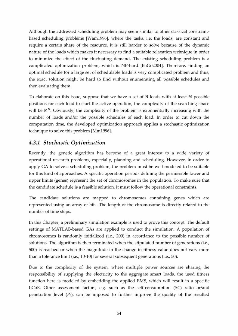
54
Although the addressed scheduling problem may seem similar to other classical constraint-
based scheduling problems [Wam1996], where the tasks, i.e. the loads, are constant and
require a certain share of the resource, it is still harder to solve because of the dynamic
nature of the loads which makes it necessary to find a suitable relaxation technique in order
to minimize the effect of the fluctuating demand. The existing scheduling problem is a
complicated optimization problem, which is NP-hard [BaGo2004]. Therefore, finding an
optimal schedule for a large set of schedulable loads is very complicated problem and thus,
the exact solution might be hard to find without enumerating all possible schedules and
then evaluating them.
To elaborate on this issue, suppose that we have a set of Ν loads with at least Μ possible
positions for each load to start the active operation, the complexity of the searching space
will be ΜΝ. Obviously, the complexity of the problem is exponentially increasing with the
number of loads and/or the possible schedules of each load. In order to cut down the
computation time, the developed optimization approach applies a stochastic optimization
technique to solve this problem [Mm1996].
4.3.1 Stochastic Optimization
Recently, the genetic algorithm has become of a great interest to a wide variety of
operational research problems, especially, planning and scheduling. However, in order to
apply GA to solve a scheduling problem, the problem must be well modeled to be suitable
for this kind of approaches. A specific operation periods defining the permissible lower and
upper limits (genes) represent the set of chromosomes in the population. To make sure that
the candidate schedule is a feasible solution, it must follow the operational constraints.
The candidate solutions are mapped to chromosomes containing genes which are
represented using an array of bits. The length of the chromosome is directly related to the
number of time steps.
In this Chapter, a preliminary simulation example is used to prove this concept. The default
settings of MATLAB-based GAs are applied to conduct the simulation. A population of
chromosomes is randomly initialized (i.e., 200) in accordance to the possible number of
solutions. The algorithm is then terminated when the stipulated number of generations (i.e.,
500) is reached or when the magnitude in the change in fitness value does not vary more
than a tolerance limit (i.e., 10-10) for several subsequent generations (i.e., 50).
Due to the complexity of the system, where multiple power sources are sharing the
responsibility of supplying the electricity to the aggregate smart loads, the used fitness
function here is modeled by embedding the applied EMS, which will result in a specific
LCoE. Other assessment factors, e.g. such as the self-consumption (SC) ratio or/and
penetration level (PL), can be imposed to further improve the quality of the resulted
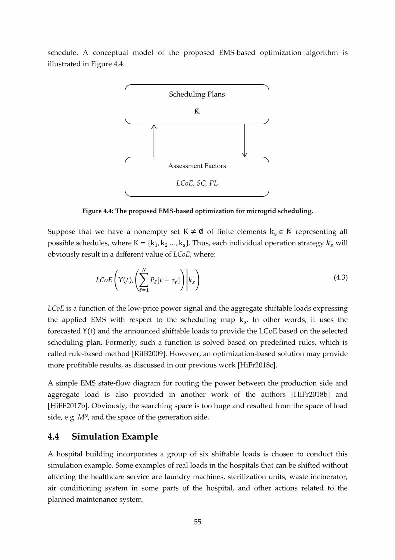
55
schedule. A conceptual model of the proposed EMS-based optimization algorithm is
illustrated in Figure 4.4.
Figure 4.4: The proposed EMS-based optimization for microgrid scheduling.
Suppose that we have a nonempty set Ƙ ≠ ∅ of finite elements ks ℕ representing all
possible schedules, where Ƙ = {k1, k2 … , ks}. Thus, each individual operation strategy 𝑘𝑠 will
obviously result in a different value of LCoE, where:
𝐿𝐶𝑜𝐸 (Υ(𝑡), (∑ 𝑃ℓ[𝑡 − ℓ]
𝑁
ℓ=1
) |𝑘𝑠) (4.3)
LCoE is a function of the low-price power signal and the aggregate shiftable loads expressing
the applied EMS with respect to the scheduling map ks. In other words, it uses the
forecasted Υ(t) and the announced shiftable loads to provide the LCoE based on the selected
scheduling plan. Formerly, such a function is solved based on predefined rules, which is
called rule-based method [RifB2009]. However, an optimization-based solution may provide
more profitable results, as discussed in our previous work [HiFr2018c].
A simple EMS state-flow diagram for routing the power between the production side and
aggregate load is also provided in another work of the authors [HiFr2018b] and
[HiFF2017b]. Obviously, the searching space is too huge and resulted from the space of load
side, e.g. MN, and the space of the generation side.
4.4 Simulation Example
A hospital building incorporates a group of six shiftable loads is chosen to conduct this
simulation example. Some examples of real loads in the hospitals that can be shifted without
affecting the healthcare service are laundry machines, sterilization units, waste incinerator,
air conditioning system in some parts of the hospital, and other actions related to the
planned maintenance system.
Scheduling Plans
Ƙ
Assessment Factors
LCoE, SC, PL
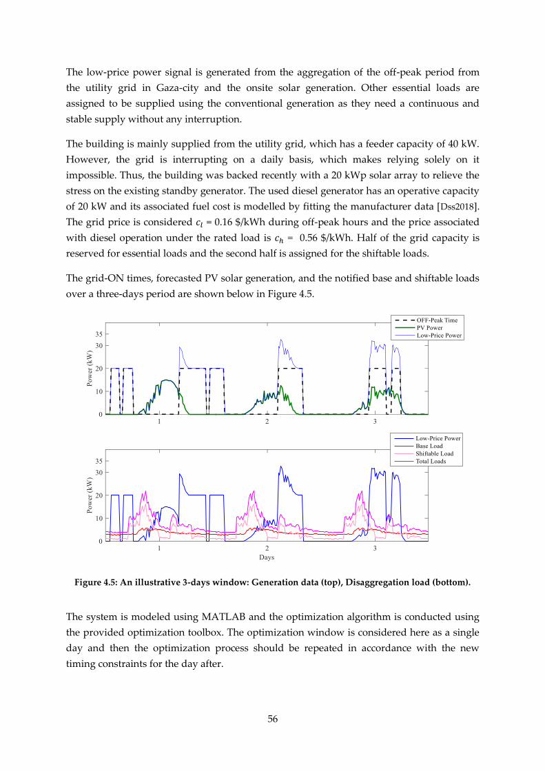
56
The low-price power signal is generated from the aggregation of the off-peak period from
the utility grid in Gaza-city and the onsite solar generation. Other essential loads are
assigned to be supplied using the conventional generation as they need a continuous and
stable supply without any interruption.
The building is mainly supplied from the utility grid, which has a feeder capacity of 40 kW.
However, the grid is interrupting on a daily basis, which makes relying solely on it
impossible. Thus, the building was backed recently with a 20 kWp solar array to relieve the
stress on the existing standby generator. The used diesel generator has an operative capacity
of 20 kW and its associated fuel cost is modelled by fitting the manufacturer data [Dss2018].
The grid price is considered 𝑐𝑙 = 0.16 $/kWh during off-peak hours and the price associated
with diesel operation under the rated load is 𝑐ℎ = 0.56 $/kWh. Half of the grid capacity is
reserved for essential loads and the second half is assigned for the shiftable loads.
The grid-ON times, forecasted PV solar generation, and the notified base and shiftable loads
over a three-days period are shown below in Figure 4.5.
Figure 4.5: An illustrative 3-days window: Generation data (top), Disaggregation load (bottom).
The system is modeled using MATLAB and the optimization algorithm is conducted using
the provided optimization toolbox. The optimization window is considered here as a single
day and then the optimization process should be repeated in accordance with the new
timing constraints for the day after.
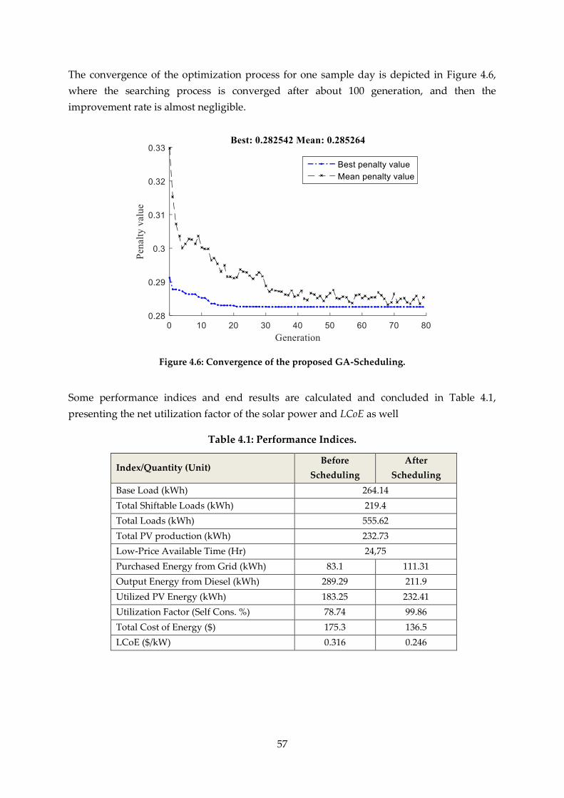
57
The convergence of the optimization process for one sample day is depicted in Figure 4.6,
where the searching process is converged after about 100 generation, and then the
improvement rate is almost negligible.
Figure 4.6: Convergence of the proposed GA-Scheduling.
Some performance indices and end results are calculated and concluded in Table 4.1,
presenting the net utilization factor of the solar power and LCoE as well
Table 4.1: Performance Indices.
Index/Quantity (Unit) Before
Scheduling
After
Scheduling
Base Load (kWh) 264.14
Total Shiftable Loads (kWh) 219.4
Total Loads (kWh) 555.62
Total PV production (kWh) 232.73
Low-Price Available Time (Hr) 24,75
Purchased Energy from Grid (kWh) 83.1 111.31
Output Energy from Diesel (kWh) 289.29 211.9
Utilized PV Energy (kWh) 183.25 232.41
Utilization Factor (Self Cons. %) 78.74 99.86
Total Cost of Energy ($) 175.3 136.5
LCoE ($/kW) 0.316 0.246
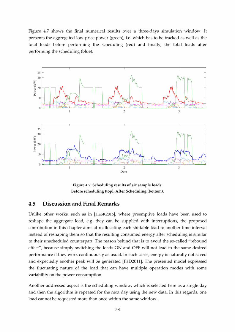
58
Figure 4.7 shows the final numerical results over a three-days simulation window. It
presents the aggregated low-price power (green), i.e. which has to be tracked as well as the
total loads before performing the scheduling (red) and finally, the total loads after
performing the scheduling (blue).
Figure 4.7: Scheduling results of six sample loads:
Before scheduling (top), After Scheduling (bottom).
4.5 Discussion and Final Remarks
Unlike other works, such as in [HabK2016], where preemptive loads have been used to
reshape the aggregate load, e.g. they can be supplied with interruptions, the proposed
contribution in this chapter aims at reallocating each shiftable load to another time interval
instead of reshaping them so that the resulting consumed energy after scheduling is similar
to their unscheduled counterpart. The reason behind that is to avoid the so-called “rebound
effect”, because simply switching the loads ON and OFF will not lead to the same desired
performance if they work continuously as usual. In such cases, energy is naturally not saved
and expectedly another peak will be generated [PaD2011]. The presented model expressed
the fluctuating nature of the load that can have multiple operation modes with some
variability on the power consumption.
Another addressed aspect is the scheduling window, which is selected here as a single day
and then the algorithm is repeated for the next day using the new data. In this regards, one
load cannot be requested more than once within the same window.

59
Otherwise, two or more identical loads with different activation constraints should be used
in order not to allow any overlapping of the operation of same load in that facility.
Formerly, the developed scheduling algorithms were adopting some scheduling policies
used in real-time processing such as Earliest Deadline First (EDF) and Least Laxity First
(LLF) which assign the tasks, e.g. loads, according to their deadlines or the slack times
[SuGD2012]. However, in renewable energy systems with versatile loads, such algorithms
still need an accurate forecasting tools and systems to handle the fluctuating nature of the
RES and the dynamic price of the grid. Therefore, the matter of prioritizing loads should
consider both: timings of the loads and their consumption level at each time slot. Obviously,
the dominants loads will be those with higher consumption and less timing flexibility than
others, which will diminish the effect of other shiftable loads but with lower consumption.
An easy-to-implement load scheduling approach based on the notified nature of the system
was proposed. Besides, a straightforward model for smart shiftable loads was introduced in
this chapter. The proposed approach has adopted the GAs to cut-down the searching space
and find the optimal schedule within a reasonable time budget. Obviously, the net
utilization of the installed PV-field is improved by more than 10% and the cost of energy is
reduced up to 78% of the original value. As presented in Table 4.1, the reduction in
purchased energy from the grid and the output power from diesel generator is substituted
after scheduling by increasing the net utilization of the solar energy and the purchased
energy from the grid as well.
Yet, there are three important topics that have not been explored and can be the subject of
future research:
(a) Reduction the capacity of the diesel generator. The economic basis for this issue
should be clearly justified through synthetic examples and much more
comprehensive simulations using real data.
(b) The incorporated energy management scheme, which will highlight the power
routing between all system components, including the static and the essential loads
which cannot be shifted in time.
(c) Online adaptation of the schedules using shorter time window instead of performing
the algorithm once per day. Thus, the improvement rate can be further increased
according to the recent measurements of the RES generation and the loads as well.

61
5 Layout Design
Water is known as a lifeblood. Nowadays, electricity is the life however. No one can deny
how electricity become essential in our daily life. The matter of power provisioning of a
system encompasses several challenges starting from selecting the appropriate energy
sources and not ending with determining the percentage share of each source to supply the
desired load demand. Yet, it would involve a complicated optimization problem, especially
when it comes to several components must be managed in a way to cover the instantaneous
demand with the least possible price. Furthermore, the capital cost of system should be
considered in order to achieve a reasonable Levelized Cost of Energy (LCoE). In this
chapter, the traditional min-max designing method will be overviewed firstly with an
introductory design example to highlight the most important technical aspects of providing a
provisioning power supply system for a specific load profile. Consequently, an optimization-
based components’ sizing method will be presented and compared with the former method to
compare the performance factors and highlight the cost savings.
5.1 Introduction
As introduced earlier, the concept of hybrid generation is promising from different
perspectives, especially to the regions around the world which have an inadequate grid
infrastructure or/and an intermittent power from the local grid and mainly depend on
backup diesel generators to supply their essential demand. Such examples are widely spread
in the Middle East, in Africa and in India with various degrees of power lack [Hi++2016].
Nevertheless, the situation becomes even more complicated when considering the expected
extra cost of fuel transportation or a breakdown of the supply chain, which may seriously
affect people’s life [Hi++2015]. Traditionally, the backup power generation systems are
mostly relying on diesel generators which are considered not only huge fuel consumers and
environmentally unfriendly, but also economically costly. Recently, with the development in
the renewable energy industry, the deployment of renewable energy resources (RES) is
expected to be a good alternative of energy at the long term. Moreover, the cooperation
between RES and diesel generators can lead to significant synergies compared with legacy
systems which are, in fact, depending only on diesel generation in case of power outages.
The most appropriate system for such situations is PV-Battery-Diesel, especially where the
grid cannot meet the load demand at every time.
5.1.1 Related works
Different search-based method have been applied to solve this problem—considering
different constraints—starting from iterative-based or exhaustive searching methods and
ending with stochastic searching methods. Regarding the topology of the designed
microgrids, the major part of the literature is dedicated to islanded or off-grid applications,
such as in [An++2015], [MuKg2011], [CsGW2012], and [Dss2018]. However, a few works
presented grid-connected applications, such as [DrBj2005], [AmBa2013], [DjBw2013] and
[Mm1996].
62
Specifically, in [DrBj2005] the authors discuss the sizing of a battery energy storage system
(BESS) for a microgrid to maximize the profit of energy trading among the microgrid and
the existing power markets. The same objective was searched for in [AmBa2013] and
[DjBw2013], but in order to size PV-Battery system considering different energy tariffs and
market policies. Other works proposed some flexibility on the demand side, where the
systems have been designed based on the worst-case condition of the net demand, such as in
[Dss2018] where the system considered was off-grid, and in [Mm1996] where the system
was connected to the grid.
5.1.2 Main Contribution
It is observed that the most of the previously proposed approaches have not included both
the operational constraints of all components and the unutilized RES. However, this work
attempts to maximize the net returns of renewable energy resources (RES) by increasing the
percentage of their utilization and penetration as well. In addition, it compromises between
the expected running costs -resulted by fuel consumption and energy purchased from the
grid- and the investment of adding new components. Besides, it makes use of an enhanced
version of the developed rule-based energy management strategy, cf. Ch 3 and integrate it
with the design approach to serve as a kernel during the optimization process.
The presented method in this chapter represents an easy-to-implement layout-design
method for medium-scale, scalable, and self-sufficient microgrids which are ready to be
interconnected with the regional grid (once existed) aiming at healing the weakened grid as
far as possible.
The main contribution is the fact that the key factors for selecting the optimum size of the
MG components cannot be reduced to just the load profile and the available renewable
generation, but also how the instantaneous power is routed in the MG. Furthermore, this
method tackles also the issue, that the decision parameters do not only concern the sizing of
the components—PV generation and battery bank (beside the existing diesel generator)—but
also the imperial switching criterion among battery, diesel generator and the main grid in
case of insufficient PV generation: that is, the lower and the upper limit of the state of charge
(SoC) at which the battery and diesel generator (or the main grid too) are switched on/off.
Lastly, the real utilization factor of RES after performing the control strategy is investigated
upon different scenarios.
5.2 Enhanced Rule-Based (RB) Operation Policy
The energy management system (EMS) is the core controller which routes the power from
different resources to supply the load in an efficient manner. Therefore, an instantaneous
power balance must be achieved as depicted in equation (5.1):
LossLGDBBPVPV PPPPPNPN (5.1)

63
where NPV and NB are the total number of photovoltaic panels and storage units,
respectively, PD is the generated power by the diesel generator, PG is the power drawn from
the grid utility, PL is the instantaneous load demand and PLoss is the total unused power, i.e.,
the lost power due to power conversion, plus the unutilized solar power.
The rule-based operation policy does not require a prediction. However, it only makes use
of the real-time measurements and grid status to determine the power route or switching
mode of the controllable components of the microgrid, basically the battery storage bank
and the generator. The operation policy is general and can be applied on all similar cases.
The power set-points for microgrid components are calculated at each time step according to
the logic rules or priorities using only the knowledge of current SoC, load, RES generation
and grid status.
A flow chart diagram of the developed operation policy in this work is shown in Figure 5.1.
Figure 5.1: Enhanced Rule-based operation policy for the proposed microgrid.
Battery Bank Master
Diesel GenSet (OFF/Standby)
(PPV < PL/η) Discharging(PPV ≥ PL/η) Charging
Diesel GenSETMaster
PL ≤ (0.85 × PD (max) = PD(Best))Use the residual capacity up to
PD(Best) to charge the battery
Keep (PD) as close as possible to PD(Best)
SoC ≤ SoCmin
SoC ≥ SoCstp
Grid (ON)
[ Supply unmet load ]Diesel GenSet [OFF]
[ Charge the battery by the residual - up to SoCstp ]
Grid (ON)Grid (OFF)

64
Some key features of this algorithm are:
• RES, i.e. Solar production is utilized in priority order: load >> storage >> dump
(unutilized).
• Load is supplied with priority order: PV >> grid >> storage >> generator.
• Battery bank is either charged by the grid during ON-grid hours or by the generator
once the load is lower than the best operation point BestGenP .
• The battery bank and the generator cannot supply the load in the same time, means
that the battery cannot operate in the discharging mode during the operation of the
generator.
Basically, this operation policy adopts a master/slave operation based on these pre-defined
rules, i.e., the highest priority is given to the renewable energy, then to the grid utility, next
to the battery storage system and, finally, to the diesel generator. Besides, discharging
process of the battery cannot occur with the operation of diesel generator concurrently. On
the other hand, the charging process of the battery can occur at times while the diesel
generator is ON.
As illustrated in Figure 5.1, PPV takes the highest priority to supply the load. Thus, once it is
insufficient, the grid takes the responsibility to supply the residual load if it is ON. In case of
insufficient renewable supply and power outage, the battery is imposed to supply the
residual load as long as its SoC is above a certain threshold SoCmin. Finally, the generator is
operated to supply the unmet load in case that SoC is less than SoCmin. To keep a higher fuel
efficiency of the diesel generator, its residual power charges the battery up to a certain limit
SoCstp if its loading factor is less than BestGenP .
Such a criterion can be met by solving equation (5.2):
τSoCSoCτnetD,PminτP stpBest
GenD
1(5.2)
where τnetD is the instantaneous unmet load by PV generation, i.e., NPVPPV . Hence, the
output power of the diesel generator is kept at its best rate as long as the remaining charge
of the battery (to reach its maximum allowable SoCstp) is more than the residual of diesel
generator. This equation applies the concept of a single-slot predictive control, where the
output power of the generator is determined based on the current measurement of the SoC
and the targeted upper limit of it, if it is going to be charged by the generator.
An example of the interactions among the microgrid components according to the enhanced
RB operation policy is explicitly illustrated in Figure 5.2.
The top figure shows the load profile (blue), available PV generation (green), and the
maximum available power from grid (yallow), where these signals represent the main inputs
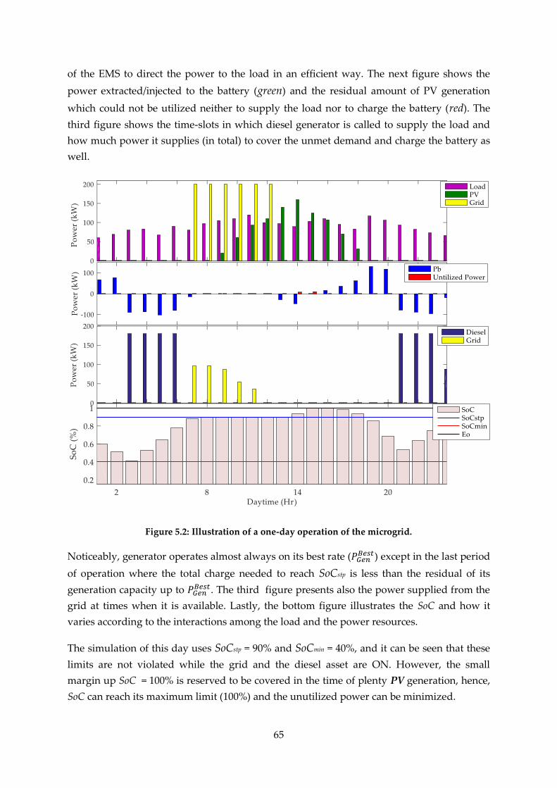
65
of the EMS to direct the power to the load in an efficient way. The next figure shows the
power extracted/injected to the battery (green) and the residual amount of PV generation
which could not be utilized neither to supply the load nor to charge the battery (red). The
third figure shows the time-slots in which diesel generator is called to supply the load and
how much power it supplies (in total) to cover the unmet demand and charge the battery as
well.
Figure 5.2: Illustration of a one-day operation of the microgrid.
Noticeably, generator operates almost always on its best rate (𝑃𝐺𝑒𝑛𝐵𝑒𝑠𝑡) except in the last period
of operation where the total charge needed to reach SoCstp is less than the residual of its
generation capacity up to 𝑃𝐺𝑒𝑛𝐵𝑒𝑠𝑡. The third figure presents also the power supplied from the
grid at times when it is available. Lastly, the bottom figure illustrates the SoC and how it
varies according to the interactions among the load and the power resources.
The simulation of this day uses SoCstp = 90% and SoCmin = 40%, and it can be seen that these
limits are not violated while the grid and the diesel asset are ON. However, the small
margin up SoC = 100% is reserved to be covered in the time of plenty PV generation, hence,
SoC can reach its maximum limit (100%) and the unutilized power can be minimized.
66
5.3 EMS-Integrated Design Method
Basically, it is crucial to find a cheaper and cleaner supply than diesel in order to cover the
needed demand of a facility at a cheaper price of energy over a long term. Besides, a
compromise should be found between the running cost and the investment capital.
The optimization algorithm employs a Genetic Algorithm (GA), which is one of the
metaheuristic stochastic optimization techniques that can provide a solution to an
optimization problem with less computational effort than iterative ones [Mm1996].
The objective function to be optimized is the total sum of the investment and running cost
over the annual cost of the system, where the running cost results mainly from the
purchased energy from the grid (in case of a grid-connected case), and the fuel consumption
by the diesel generator, and the investment cost depends mainly on the instalment plan or
the installation cost of the components (PV panels, Battery bank, Diesel Generator and the
inverter), plus the maintenance and replacement cost of some components such as batteries.
Equation (5.3) represents the mathematical formulation of the whole cost function, equations
(5.4) and (5.5) correspond to the detailed mathematical formulation of the investment and
running costs ( invC , runC ), respectively.
runinvtot CCC (5.3)
DGBest
DGBatBPVPVinv CPCNCNC (5.4)
ggcfrun ECFCC (5.5)
PVN and BN are the total number of PV panels and storage units, 𝑃𝐺𝑒𝑛𝐵𝑒𝑠𝑡 is the maximum
capacity of diesel generator, 𝐶𝑃𝑉, 𝐶𝐵𝑎𝑡, 𝐶𝐷𝐺 are the prices of a single PV panel, a single
storage unit and the corresponding diesel generator, respectively.
The parameters Cg, Eg and Cf are the energy price per kWh from the grid, the total energy
purchased from grid and fuel price per liter including the costs of transportation and
logistics.
In case of isolated MGs, the total purchase from grid Eg will be zero and hence, the run cost
will merely be resulted from the diesel generator.
A pseudo-code of the applied GA, including a specific decision on the appropriateness of
each candidate 5-tuple C of decision variables (Step 4), is depicted in Figure 5.3. Each
appropriate candidate is evaluated over a one-year load and weather profile to find out the
best fitness function (Equation 5.6).
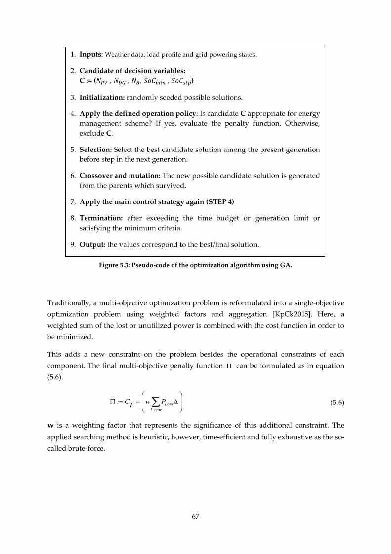
67
Figure 5.3: Pseudo-code of the optimization algorithm using GA.
Traditionally, a multi-objective optimization problem is reformulated into a single-objective
optimization problem using weighted factors and aggregation [KpCk2015]. Here, a
weighted sum of the lost or unutilized power is combined with the cost function in order to
be minimized.
This adds a new constraint on the problem besides the operational constraints of each
component. The final multi-objective penalty function can be formulated as in equation
(5.6).
year 1
LossPwT
C: (5.6)
w is a weighting factor that represents the significance of this additional constraint. The
applied searching method is heuristic, however, time-efficient and fully exhaustive as the so-
called brute-force.
1. Inputs: Weather data, load profile and grid powering states.
2. Candidate of decision variables:
C := (𝑁𝑃𝑉 , 𝑁𝐷𝐺 , 𝑁𝐵, 𝑆𝑜𝐶𝑚𝑖𝑛 , 𝑆𝑜𝐶𝑠𝑡𝑝)
3. Initialization: randomly seeded possible solutions.
4. Apply the defined operation policy: Is candidate C appropriate for energy
management scheme? If yes, evaluate the penalty function. Otherwise,
exclude C.
5. Selection: Select the best candidate solution among the present generation
before step in the next generation.
6. Crossover and mutation: The new possible candidate solution is generated
from the parents which survived.
7. Apply the main control strategy again (STEP 4)
8. Termination: after exceeding the time budget or generation limit or
satisfying the minimum criteria.
9. Output: the values correspond to the best/final solution.

68
5.3.1 Searching Space
The search space of the problem is obviously very large. Considering NPV solar panels, NDG
set of the diesel generators, and NB battery storage units with NSoC different levels of SoCmin
and SoCstp (which we declared in advance) to choose from, the number of iterations would
reach (NPV×NDG×NB×NSoC×NSoC) of iterations, each requiring k evaluations of Equ. (5.1) to
(5.6) if an iterative method, e.g. brute-force, is chosen to check all possible combinations (as
done, e.g., in [An++2015]); k is the number of total time slots among the year (here k :=
6×8760 = 52560). Yet, the checking process includes also the implicit or the integrated
operation policy which has been applied to figure out the real efficiency of the system. For
that reason, the GA is chosen as it enables the exploration of a wide range of allotted
elements in a much shorter time.
In our case, less than 80 generations were examined until they converged to a solution (here:
just a few minutes of computation time).
5.4 Design Example
The essential load of a building of an outpatient in Gaza city is taken as a case study where
daily grid outages are common routine since years [Hi++2015]. A fraction of the load profile
is chosen to conduct the simulation where the maximum peak during one year is 71.2 kW
and minimum load is 25.3 kW with a mean consumption of 42.8 kW and 10.4 kW of
standard deviation [MuKg2011].
A powerful tool to describe the chosen load profile is the load duration curve (LDC), by
which, the aforementioned statistical information can be described clearly, where the values
of the power profile are sorted in a descending order, as depicted in Figure 5.4.
Figure 5.4: Load duration curve (LDC) of the load over one year.
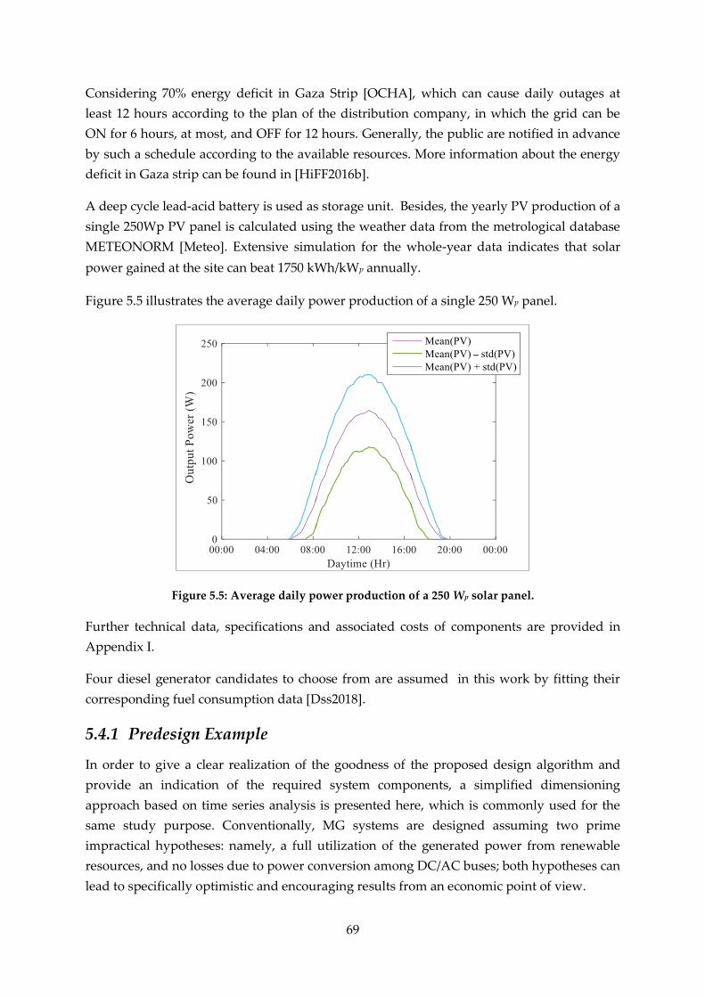
69
Considering 70% energy deficit in Gaza Strip [OCHA], which can cause daily outages at
least 12 hours according to the plan of the distribution company, in which the grid can be
ON for 6 hours, at most, and OFF for 12 hours. Generally, the public are notified in advance
by such a schedule according to the available resources. More information about the energy
deficit in Gaza strip can be found in [HiFF2016b].
A deep cycle lead-acid battery is used as storage unit. Besides, the yearly PV production of a
single 250Wp PV panel is calculated using the weather data from the metrological database
METEONORM [Meteo]. Extensive simulation for the whole-year data indicates that solar
power gained at the site can beat 1750 kWh/kWp annually.
Figure 5.5 illustrates the average daily power production of a single 250 Wp panel.
Figure 5.5: Average daily power production of a 250 Wp solar panel.
Further technical data, specifications and associated costs of components are provided in
Appendix I.
Four diesel generator candidates to choose from are assumed in this work by fitting their
corresponding fuel consumption data [Dss2018].
5.4.1 Predesign Example
In order to give a clear realization of the goodness of the proposed design algorithm and
provide an indication of the required system components, a simplified dimensioning
approach based on time series analysis is presented here, which is commonly used for the
same study purpose. Conventionally, MG systems are designed assuming two prime
impractical hypotheses: namely, a full utilization of the generated power from renewable
resources, and no losses due to power conversion among DC/AC buses; both hypotheses can
lead to specifically optimistic and encouraging results from an economic point of view.

70
In addition, many approaches do not include the energy management scheme during
optimization. By contrast, the proposed design herein is optimized taking into account the
applied operation policy and realistic power conversion efficiencies, which together play the
key role in determining the realistic percentage of utilized renewable energy.
Obviously, using the integration of equ. (5.1), energy balance of the system must be
achieved. By which, capacities of each of diesel generator and the bi-directional inverter can
be roughly estimated, as shown in Equ. (5.7):
LossLGDBPV EEEEEE (5.7)
Simply, the resulting net power demand, after subtracting available PV power from the load
profile should be supplied by either by grid or diesel generator in addition to the assistance
of battery storage. Subsequently, by defining the desired penetration level ( in equ. 5.8) of
the renewables, i.e. PV, the lower bounds of solar panels can be determined, that is,
considering zero losses due to power conversion or/and applied operation policy. After that,
other resources can supply the residual load, which has not been supplied by the PVs.
00
dt)(Pdt)(P LPV (5.8)
Besides, maximum power ratings of the battery, diesel generator and power inverter must
be able to handle the peak load. Generally, different manufacturers have their different
recommendations and preferences of the charging/discharging characteristics. Mostly, in
order to assure healthy operating conditions for the battery, maximum throughput rate must
not exceed a certain value C/(5 h); C is the battery capacity in Ampere hours (Ah).
Other considerations such as supply of reactive power or fault tolerance considerations,
would of course lead to further increased capacities and power ratings.
Findings of the components after a predesign phase are listed below in Table 5-1:
Table 5-1: Predesign Microgrid Components
Parameter Nomenclature Value (s)
𝑁𝐵 Number of storage units 65 Storage units
𝑁𝑃𝑉 Number of PV panels 857 Panels
𝑃𝐷𝐺𝑚𝑎𝑥 Diesel generator capacity 100 kW
𝑃𝑖𝑛𝑣 Ratings of the power inverter 100 kVA
It is worth to mention here, that predesign phase assumes a full penetration of solar energy
which can hardly be achieved in such circumstances. In order to verify the actual
penetration level of such selected components, the operation policy must be applied. These
findings will be presented in details in the next subsection.
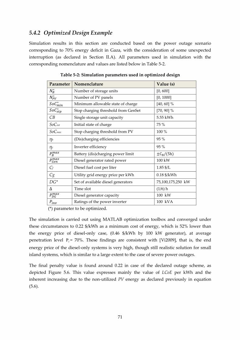
71
5.4.2 Optimized Design Example
Simulation results in this section are conducted based on the power outage scenario
corresponding to 70% energy deficit in Gaza, with the consideration of some unexpected
interruption (as declared in Section II.A). All parameters used in simulation with the
corresponding nomenclature and values are listed below in Table 5-2.
Table 5-2: Simulation parameters used in optimized design
Parameter Nomenclature Value (s)
𝑁𝐵∗ Number of storage units [0, 600]
𝑁𝑃𝑉∗ Number of PV panels [0, 1000]
𝑆𝑜𝐶𝑚𝑖𝑛∗ Minimum allowable state of charge [40, 60] %
𝑆𝑜𝐶𝑠𝑡𝑝∗ Stop charging threshold from GenSet [70, 90] %
CB Single storage unit capacity 5.55 kWh
SoCint Initial state of charge 75 %
SoCmax Stop charging threshold from PV 100 %
ηb (Dis)charging efficiencies 95 %
ηc Inverter efficiency 95 %
𝑃𝐵𝑚𝑎𝑥 Battery (dis)charging power limit ±CB/(5h)
𝑃𝐺𝑒𝑛𝑚𝑎𝑥 Diesel generator rated power 100 kW
Cf Diesel fuel cost per liter 1.85 $/L
Cg Utility grid energy price per kWh 0.18 $/kWh
DG* Set of available diesel generators 75,100,175,250 kW
∆ Time slot (1/6) h
𝑃𝐷𝐺𝑚𝑎𝑥 Diesel generator capacity 100 kW
𝑃𝑖𝑛𝑣 Ratings of the power inverter 100 kVA
(*) parameter to be optimized.
The simulation is carried out using MATLAB optimization toolbox and converged under
these circumstances to 0.22 $/kWh as a minimum cost of energy, which is 52% lower than
the energy price of diesel-only case, (0.46 $/kWh by 100 kW generator), at average
penetration level = 70%. These findings are consistent with [Vi2009], that is, the end
energy price of the diesel-only systems is very high, though still realistic solution for small
island systems, which is similar to a large extent to the case of severe power outages.
The final penalty value is found around 0.22 in case of the declared outage scheme, as
depicted Figure 5.6. This value expresses mainly the value of LCoE per kWh and the
inherent increasing due to the non-utilized PV energy as declared previously in equation
(5.6).

72
Figure 5.6: Convergence of penalty function over GA generations.
Further advantage of the algorithm that is identifying the optimum operating points of the
battery storage where the switching to the generator should be done and vice versa. These
findings of the optimized component of the MG under the aforementioned conditions, that
minimizes the LCoE over the 20-years evaluation period, are listed in below in Table 5-3.
Table 5-3: Optimized Microgrid Configuration
Parameter Nomenclature Value (s)
𝑁𝐵 Number of storage units 140 Storage units
𝑁𝑃𝑉 Number of PV panels 922 Panels
𝑃𝐷𝐺𝑚𝑎𝑥 Diesel generator capacity 100 kW
𝑃𝑖𝑛𝑣 Ratings of the power inverter 100 kVA
𝑆𝑜𝐶𝑚𝑖𝑛∗ Minimum allowable state of charge 40 %
𝑆𝑜𝐶𝑠𝑡𝑝∗ Stop charging threshold from GenSet 89 %
The annual purchased energy and fuel savings in case of the proposed system is listed below
in Table 5-4. The results are then compared with the old baseline configuration, which
depends merely on diesel generator as a backup resource in addition to the interrupting
grid.
Table 5-4: Annual Purchased Energy and Fuel Savings
Parameter Legacy System Microgrid Design
Purchased energy from grid (MWh) 124,98 116,12
Gross purchasing from grid ($×103) 22,45 20,90
Total fuel consumption (L×103) 80,98 3,31
Operation Hours (Hr) 5840 153
Total fuel costs ($×103) 149,8 6,12
Purchased energy from grid (MWh) 124,98 116,12
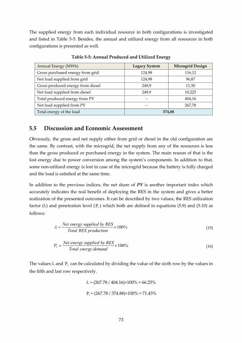
73
The supplied energy from each individual resource in both configurations is investigated
and listed in Table 5-5. Besides, the annual and utilized energy from all resources in both
configurations is presented as well.
Table 5-5: Annual Produced and Utilized Energy
Annual Energy (MWh) Legacy System Microgrid Design
Gross purchased energy from grid 124,98 116,12
Net load supplied from grid 124,98 96,87
Gross produced energy from diesel 249,9 11,50
Net load supplied from diesel 249,9 10,225
Total produced energy from PV – 404,16
Net load supplied from PV – 267,78
Total energy of the load 374,88
5.5 Discussion and Economic Assessment
Obviously, the gross and net supply either from grid or diesel in the old configuration are
the same. By contrast, with the microgrid, the net supply from any of the resources is less
than the gross produced or purchased energy in the system. The main reason of that is the
lost energy due to power conversion among the system’s components. In addition to that,
some non-utilized energy is lost in case of the microgrid because the battery is fully charged
and the load is satisfied at the same time.
In addition to the previous indices, the net share of PV is another important index which
accurately indicates the real benefit of deploying the RES in the system and gives a better
realization of the presented outcomes. It can be described by two values, the RES utilization
factor () and penetration level ( ) which both are defined in equations (5.9) and (5.10) as
follows:
%production RESTotal
RESby suppliedenergyNet100 (15)
%demandenergyTotal
RESby suppliedenergyNetP 100 (16)
The values and can be calculated by dividing the value of the sixth row by the values in
the fifth and last row respectively.
= (267.78 / 404.16)×100% ≈ 66.25%
= (267.78 / 374.88)×100% ≈ 71.43%

74
As depicted below in Figure 5.7, a pie chart illustrates the net share of each resource in both
situations (Grid-Diesel and Grid-Microgrid). Meanwhile, the penetration level ( ) of PV
array in the new configuration is marked with a green color.
(a) (b)
(a) Baseline (b) Grid-connected MG
Figure 5.7: The net energy share of each power source.
It is also remarkable that installing less RES, e.g. PVs leads to benefit from a plentiful
generated energy, meaning that, less rejected or unutilized energy. This is obvious because
RES, in that case, lies mostly under the load demand, which allows to be directly taken by
the load.
In contrast, seeking a high penetration level leads to a relatively high rejected RES and thus,
low utilization factor, because the residual RES will be either redirected to the battery or
even rejected. This phenomena can be illustrated using 3-days power profiles of 600 PV
panels, grid line and load demand, as shown in Figure 5.8.
Figure 5.8: Power profiles of 600 PVs, interrupted grid and load.

75
It is evident that most of the generated PV power can be directly absorbed by the load once
it is less than demand. However, in case of residual generation, it will be redirected to
charge battery for example.
Of course, this will result in more losses due to power conversion. Thus, oversized PV units
may lead to higher penetration levels, but not necessarily to more economic designs.
Aside from the technical indices, the net present value (NPV) is chosen to analyze the
profitability of the proposed project. It indicates the algebraic sum of the net cash flows over
a project period. It can be formulated as in equation (5.11).
N
n0
Cnr1
nC
NPV1
(17)
Where: n {1, 2, 3,…, N} points to the year; N = 20 years. C0 is the first installment of the
project (here it is the investment cost of PV panels and storage units). Cn is the total cash
flow over year n, 𝑟 is the discount rate. The yearly net cash flow is resulted from the
revenues minus the running costs and capital investment. Obviously, revenues come from
the considered price for supplying the load by RES. Contrariwise, the running costs are
dominated by the costs of supplied energy from grid and diesel generator in addition to the
replacement costs of the batteries. In addition, extra revenue is added as an incentive to
reduce the dependency on the grid and diesel fuel. Considering the resulted components
(see Table 5-3) with the corresponding declared prices and two times replacements of the
batteries, the NPV is described in Figure 5.9.
Figure 5.9: Net Present Value of the proposed microgrid.
The graph shows that the net return will beat the payments after the eighth year, which
makes the proposed system profitable for the considered case.

76
5.6 Conclusion and Final Remarks
This chapter presents a straight-forward method to provide an optimal layout design of a
microgrid including PV array, ESS and Diesel asset. The presented method is general and
can be applied for deigning a grid-connected or an isolated microgrid, considering a
complete power outage. The method is appropriate for societies and communities subject to
frequent grid outages where, in times of grid outage, the load is supplied merely by diesel
generators, which consume a huge amount of fuel. A case study of a hospital building
subject to severe power outages has been presented.
However, with the microgrid, the annual payments of installation and replacement count
75×103 US-$, but the long-term annual savings will be 145×103 US-$, which means that the
net annual saving will be about 70×103 US-$, that is half the fuel cost in the old
configuration. In addition, a very reasonable utilization of RES can be achieved with
microgrid (UF = 66.25%). Besides, a high RES penetration level can be achieved ( Pℓ =
71.43%).
Furthermore, it is noticed that the optimal selection of components depends primarily on
the adopted operation policy in addition to the gross energy produced by RES rather than
on the initial prices of the components only. Installing such RES in microgrids can be done
gradually, and expectedly, the savings will increase progressively.

78
6 Conclusion and Outlook
This work addressed in the first place the PV-Battery-Diesel Microgrid system as a
resolution for one of the most emerging electrification problems, especially in the
developing countries where the operational costs of conventional alternatives are
unimaginable.
Mainly, two important topics were comprehensively covered in the course of this work. The
first one was on the developing of an efficient EMS based on the basic modeling of each
system component. For this topic, three different EMSs were presented and discussed with a
real-case scenario. A former rule-based was discussed firstly and the enhancement potential
to increase the efficiency of the system was successfully highlighted. Afterwards, two
optimization-based EMS using the prediction of were presented. The offline solution is
firstly conducted assuming a perfect prediction and then the adaptation was carried out by
imposing some errors on the predicted data. The optimization goal aims at not only
minimizing the running costs but also maximizing the net utilization of the clean solar
energy. The proposed solution adopted the former Dynamic Programming method for
tracking the least cost operation strategy. However, a relaxation technique was proposed to
speed up the optimization process and reduce the search space. Besides, another form of
energy management was presented in this work concerning the demand side in the smart
grid environment, where the loads can be predicted or notified in advance. An optimization-
based load scheduling approach was presented assuming the predictability of a group of
shiftable load. The scheduling approach considers the involved EMS of the generation side
and seeks to minimize the LCoE in accordance with the permissible operation time of the
considered loads.
The second topic of this thesis discussed the issue of selecting the capacity of each
component of the MG that will lead to the least cost of energy. The need for a hybrid system
was elaborated using a practical power outage scenario. This approach differs from other
predecessor methods in particular with the consideration of the applied EMS, by which the
effective utilization of solar energy can be varied and thus, the resulted capacity might be
oversized. It was observed that the components’ sizing depends primarily on the adopted
EMS in addition to the gross energy produced by PV rather than on the initial prices of the
components only.
The percentage of fuel reduction using the optimization-based EMS exceeded 25% in case of
accurate prediction and was about 18% in case of uncertain prediction. Depending on the
accuracy of the prediction, the proposed optimization-based approaches could maximize the
net utilized PV energy up to about 90% and thus, it can be concluded that such methods can
result in not only economic benefits but also in a more efficient operation in terms of solar
energy utilization.

79
Additionally, simulation results could clearly indicate the advantage of performing such
analyses before developing such EMS for microgrid systems or deploying new components
for the purpose of solving electrification problems to assist the legacy backup power
systems, e.g. in this case PV and Battery assist diesel Generator).
As a future prospect, it can be said that some further studies for the systems could be carried
out. First of all, it would be interesting to apply the results of the research on a specific
battery models and PV modules. Moreover, as with the aging mechanism of the considered
battery units, further investigation might be helpful for complicated strategies with dynamic
load behavior. Additionally, further operational scenario of the future microgrid systems
including Electric Vehicles and responsive loads could be an interesting research area,
especially when considering the matter of scheduling different energy sources jointly with
this kind of demand.
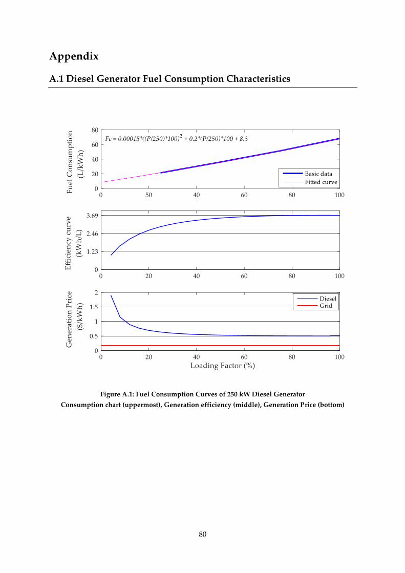
80
Appendix
A.1 Diesel Generator Fuel Consumption Characteristics
Figure A.1: Fuel Consumption Curves of 250 kW Diesel Generator
Consumption chart (uppermost), Generation efficiency (middle), Generation Price (bottom)

81
A.2 Components’ Initial Costs and Specifications
The deployed battery storage unit is a Trojan battery model IND17-6V adopted from
[Yu++2014]. It has a 5.55 kWh capacity at 20-h discharging rate and a relatively long lifetime
under a low SoC, i.e. 2200 cycles at 40% SoC with a nominal price of 1400 $. Its maximum
(dis)charging is considered 1/5 of the capacity within 1 h to keep healthy operating
conditions. Considering one cycle per day, its annual capital cost is:
1430 ($) × [365 (cycles/yr) / 2200 (cycles)] = 237 ($/yr).
The used solar generator is a 250Wp PV panel which is the kernel of the PV array and has a
price of 1.9$/Wp including the installation, corresponding power electronics, and converters
for voltage regulation and adaption among power bus bars. Assuming a 20-years warranty
over the project lifetime, the annual price of each panel is:
[1.9 ($/Wp) × 250 (Wp)] / 20 (yr) = 24 ($/yr).
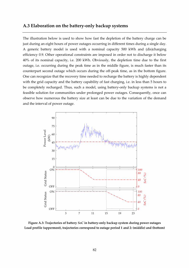
82
A.3 Elaboration on the battery-only backup systems
The illustration below is used to show how fast the depletion of the battery charge can be
just during an eight hours of power outages occurring in different times during a single day.
A generic battery model is used with a nominal capacity 500 kWh and (dis)charging
efficiency 0.9. Other operational constraints are imposed in order not to discharge it below
40% of its nominal capacity, i.e. 200 kWh. Obviously, the depletion time due to the first
outage, i.e. occurring during the peak time as in the middle figure, is much faster than its
counterpart second outage which occurs during the off-peak time, as in the bottom figure.
One can recognize that the recovery time needed to recharge the battery is highly dependent
with the grid capacity and the battery capability of fast charging, i.e. in less than 5 hours to
be completely recharged. Thus, such a model, using battery-only backup systems is not a
feasible solution for communities under prolonged power outages. Consequently, once can
observe how numerous the battery size at least can be due to the variation of the demand
and the interval of power outage.
Figure A.3: Trajectories of battery SoC in battery-only backup system during power outages
Load profile (uppermost), trajectories correspond to outage period 1 and 2: (middle) and (bottom)
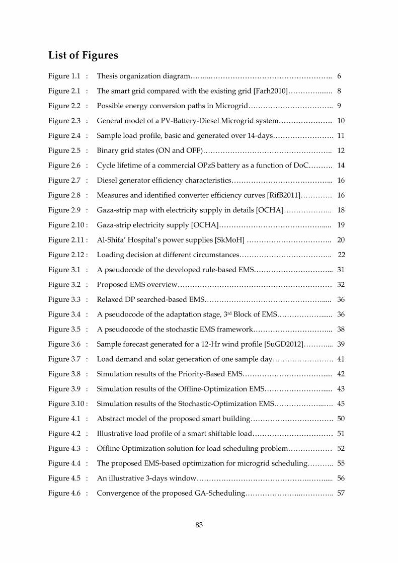
83
List of Figures
Figure 1.1 : Thesis organization diagram……...………………………………………….. 6
Figure 2.1 : The smart grid compared with the existing grid [Farh2010]…………........ 8
Figure 2.2 : Possible energy conversion paths in Microgrid…………………………….. 9
Figure 2.3 : General model of a PV-Battery-Diesel Microgrid system…………………. 10
Figure 2.4 : Sample load profile, basic and generated over 14-days……………………. 11
Figure 2.5 : Binary grid states (ON and OFF)…………………………………………….. 12
Figure 2.6 : Cycle lifetime of a commercial OPzS battery as a function of DoC………. 14
Figure 2.7 : Diesel generator efficiency characteristics…………………………………... 16
Figure 2.8 : Measures and identified converter efficiency curves [RifB2011]…………. 16
Figure 2.9 : Gaza-strip map with electricity supply in details [OCHA]……………….. 18
Figure 2.10 : Gaza-strip electricity supply [OCHA]……………………………………..... 19
Figure 2.11 : Al-Shifa’ Hospital’s power supplies [SkMoH] …………………………….. 20
Figure 2.12 : Loading decision at different circumstances……………………………….. 22
Figure 3.1 : A pseudocode of the developed rule-based EMS…………………………... 31
Figure 3.2 : Proposed EMS overview……………………………………………………… 32
Figure 3.3 : Relaxed DP searched-based EMS…………………………………………..... 36
Figure 3.4 : A pseudocode of the adaptation stage, 3rd Block of EMS………………...... 36
Figure 3.5 : A pseudocode of the stochastic EMS framework…………………………... 38
Figure 3.6 : Sample forecast generated for a 12-Hr wind profile [SuGD2012]……….... 39
Figure 3.7 : Load demand and solar generation of one sample day……………………. 41
Figure 3.8 : Simulation results of the Priority-Based EMS……………………………..... 42
Figure 3.9 : Simulation results of the Offline-Optimization EMS……………………..... 43
Figure 3.10 : Simulation results of the Stochastic-Optimization EMS………………...…. 45
Figure 4.1 : Abstract model of the proposed smart building……………………………. 50
Figure 4.2 : Illustrative load profile of a smart shiftable load…………………………… 51
Figure 4.3 : Offline Optimization solution for load scheduling problem……………… 52
Figure 4.4 : The proposed EMS-based optimization for microgrid scheduling……….. 55
Figure 4.5 : An illustrative 3-days window……………………………………….……..... 56
Figure 4.6 : Convergence of the proposed GA-Scheduling…………………..………….. 57
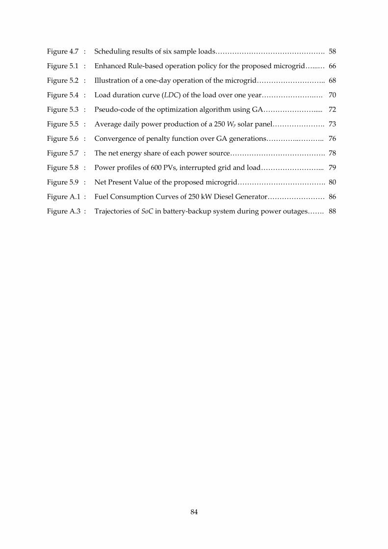
84
Figure 4.7 : Scheduling results of six sample loads………………………………………. 58
Figure 5.1 : Enhanced Rule-based operation policy for the proposed microgrid…...… 66
Figure 5.2 : Illustration of a one-day operation of the microgrid……………………….. 68
Figure 5.4 : Load duration curve (LDC) of the load over one year………………….…. 70
Figure 5.3 : Pseudo-code of the optimization algorithm using GA…………………..... 72
Figure 5.5 : Average daily power production of a 250 Wp solar panel…………………. 73
Figure 5.6 : Convergence of penalty function over GA generations…………..……….. 76
Figure 5.7 : The net energy share of each power source…………………………………. 78
Figure 5.8 : Power profiles of 600 PVs, interrupted grid and load……………………... 79
Figure 5.9 : Net Present Value of the proposed microgrid………………………………. 80
Figure A.1 : Fuel Consumption Curves of 250 kW Diesel Generator…………………… 86
Figure A.3 : Trajectories of SoC in battery-backup system during power outages……. 88
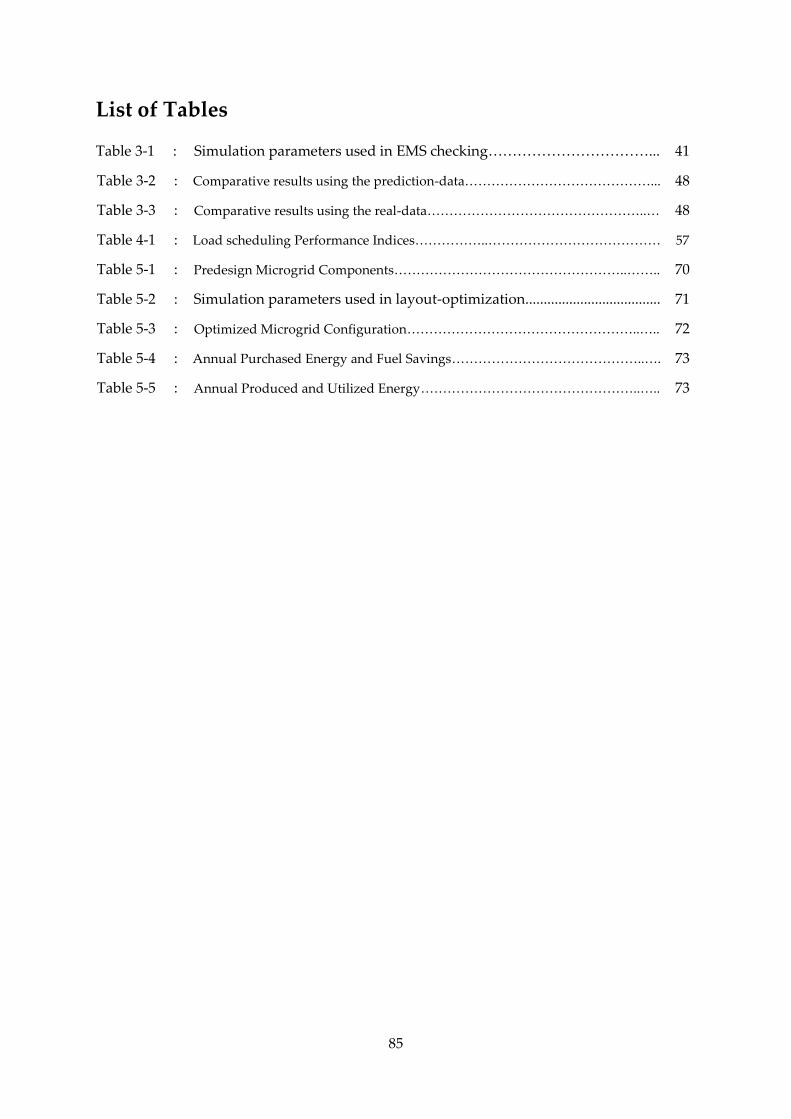
85
List of Tables
Table 3-1 : Simulation parameters used in EMS checking……………………………... 41
Table 3-2 : Comparative results using the prediction-data……………………………………... 48
Table 3-3 : Comparative results using the real-data…………………………………………..… 48
Table 4-1 : Load scheduling Performance Indices……………..………………………………… 57
Table 5-1 : Predesign Microgrid Components……………………………………………..…….. 70
Table 5-2 : Simulation parameters used in layout-optimization..................................... 71
Table 5-3 : Optimized Microgrid Configuration……………………………………………..….. 72
Table 5-4 : Annual Purchased Energy and Fuel Savings……………………………………..…. 73
Table 5-5 : Annual Produced and Utilized Energy…………………………………………..….. 73
86
Bibliography
Publications of the Author
[Hi++2015] Hijjo, M.; Bauer, P.; Felgner, F.; Frey, G.: Energy Management systems for
Hospitals in Gaza-strip. 2015 IEEE Global Humanitarian Technology Conference
(GHTC), Seattle, WA, 2015, pp. 18-25.
[Hi++2016] Hijjo, M.; Felgner, F.; Meiers, J.; Frey, G.: Energy Management for Islanded
Buildings Integrating Renewables and Diesel Generators. 2016 IEEE PES
PowerAfrica, Livingstone, 2016, pp. 62-66.
[HiFF2016a] Hijjo, M.; Felgner, F.; Frey, G.: Energy Management Scheme for Buildings Subject
to Planned Grid Outages. 2016 International Conference on Smart Cities Solutions
(ICSCS 2016), Gaza, Palestine, Aug. 2016. Received ICSCS 2016 Best Paper
Award.
[HiFF2016b] Hijjo, M.; Felgner, F.; Frey, G.: Energy Management Scheme for Buildings Subject
to Planned Grid Outages. Journal of Engineering Research and Technology, Vol.
3, No. 3 (2016), pp. 58-65, ISSN: 2312-2307. Chosen to be published in JERT after the
ICSCS 2016 conference
[HiFF2017a] Hijjo, M.; Felgner, F.; Frey, G.: PV-Battery-Diesel Microgrid Design for Buildings
Subject to Severe Power Outages. 2017 IEEE PES PowerAfrica, Accra, 2017, pp.
280-285.
[HiFF2017b] Hijjo, M.; Felgner, F.; Frey, G.: PV-Battery-Diesel Microgrid Layout Design Based
on Stochastic Optimization. 2017 6th International Conference on Clean Electrical
Power (ICCEP), Santa Margherita Ligure, 2017, pp. 30-35
[HiFr2018a] Hijjo, M.; Frey, G.: Multi-Objective Optimization for Scheduling Isolated
Microgrids. 2018 IEEE International Conference on Industrial Technology (ICIT),
Lyon, 2018, pp. 1037-1042.
[HiFr2018b] Hijjo, M.; Frey, G.: Battery Management System in Isolated Microgrids
Considering Forecast Uncertainty. 2018 9th International Renewable Energy
Congress (IREC), Hammamet, 2018, pp. 1-6.
[HiFr2018c] Hijjo, M.; Frey, G.: Stochastic Optimization Framework for Scheduling Isolated
Microgrids. 2018 19th IEEE Mediterranean Electrotechnical Conference
(MELECON), Marrakech, Morocco, 2018, pp. 149-154. Received MELECON 2018
Best Paper Award.
[HiFr2018d] Hijjo, M.; Frey, G.: Scheduling Framework for Smart Loads in Modern Buildings
Based on Metaheuristic Optimization. 2018 15th International Conference on
Informatics in Control, Automation and Robotics (ICINCO), Porto, Portugal, 2018
[HiFr2018f] Hijjo, M.; Frey, G.: Forecast-Driven Power Planning Approach for Microgrids
Incorporating Smart Loads Using Stochastic Optimization. 2018 International
Conference on Smart Energy Systems and Technologies (SEST), University of
Sevilla, Sevilla, Spain, 2018. [Accepted]

87
Internal Posters
[P2016] Hijjo, M.; Felgner, F.; Frey, G.: Microgrid Energy Management for Buildings
Subject to Grid Outages. Poster Presentation at the Doktorandentag, Saarland
University, 2016, Best poster prize from the Deanship of Naturwissenschaftlich-
Technischen Fakultät der Universität des Saarlandes.
[P2017] Hijjo, M.; Frey, G.: Microgrid Layout Design for Cost Minimization in
Conventional Diesel Backup Systems. Poster Presentation at the Doktorandentag,
Saarland University, 2017. Best poster prize from the Deanship of
Naturwissenschaftlich-Technischen Fakultät der Universität des Saarlandes.
88
References
[NjM2016] Njore, Mark M.. 2016. West Bank and Gaza - Energy efficiency action plan for
2020-2030 (English). Washington, D.C. : World Bank Group.
http://documents.worldbank.org/curated/en/851371475046203328/West-Bank-and-
Gaza-Energy-efficiency-action-plan-for-2020-2030
[EEG2017] Gesetz zur Einführung von Ausschreibungen für Strom aus erneuerbaren
Energien und zu weiteren Änderungen des Rechts der erneuerbaren Energien
(EEG 2017), Bundesrat Drucksache 355/16, 08.07.16
[NEEAP] National Energy Efficiency Action Plan (NEEAP) for Palestine, Palestinian Energy
Authority, 2011-2013
[FvL2018] Fthenakis V.; Lynn P.: Electricity from Sunlight: Photovoltaic-Systems Integration
and Sustainability, 2nd Edition. Wiley 2018
[Lr2002] Lasseter, R.: Microgrids. Power Engineering Society Winter Meeting. IEEE 2002
[DoE2011] Microgrid Exchange Group. DoE Microgrid Workshop Report. Aug 2011
[Hn2007] Hatziargyriou N.; Asano H.; Iravani R.; Marnay C.: Microgrids, in IEEE Power
and Energy Magazine, vol. 5, no. 4, pp. 78-94, July-Aug. 2007.
[VaT2013] Vandoorn, T.; Vasquez, J.; De Kooning, J.; Guerrero, J.; Vandevelde, L.:
Microgrids: Hierarchical Control and an Overview of the Control and Reserve
Management Strategies, in IEEE Industrial Electronics Magazine, vol. 7, no. 4, pp.
42-55, Dec. 2013.
[StAj2015] Stetz T.; Appen J.; Niedermeyer F.; Scheibner G.; Sikora R.; Braun M.: Twilight of
the Grids: The Impact of Distributed Solar on Germany’s Energy Transition, in
IEEE Power and Energy Magazine, vol. 13, no. 2, pp. 50-61, March-April 2015.
[Farh2010] Farhangi, H.: The path of the smart grid, in IEEE Power and Energy Magazine,
vol. 8, no. 1, pp. 18-28, January-February 2010.
[DrBj2005] Dufo-Lopez, R.; Bernal-Agustin, JL.: Design and Control Strategies of PV-Diesel
Systems Using Genetic Algorithms. Solar Energy Vol. 79, Issue 1, pp. 33-46, 2005.
[SmA2015] Saleh, M.; Althaibani, A.; Y. Mhandi, E.; Mohamed, A.: Impact of clustering
microgrids on their stability and resilience during blackouts, 2015 International
Conference on Smart Grid and Clean Energy Technologies (ICSGCE), Offenburg,
2015, pp. 195-200.
[VirT2007] Consortium on Energy Restructuring. Introduction to Distributed Generation,
Virginia Tech. 2007. Retrieved 26 August 2018.
[OCHA] United Nations Office for Coordination of Humanitarian Affairs
[CsGW2012] Chen, S. X.; Gooi, H. B.; Wang, M. Q.: Sizing of Energy Storage for Microgrids.
IEEE Transactions on Smart Grid, vol. 3, no. 1, pp. 142-151, March 2012.

89
[CERTS2003]
[PeBo2011]
[PwrSnc]
[MaY2014]
[Jen2008]
[MoP2014]
[VreP2011]
[OCHA2017]
[An++2015]
[ArYn2012]
[MuKg2011]
[AmBa2013]
Lasseter, R.; Akhil, A.; Marnay, C.; Stephens, J.; Dagle, J.; Guttromson, R.;
Meliopoulous S.; Yinger R.; Eto J.: Integration of Distributed Energy Resources:
The CERTS MicroGrid Concept. CERTS, 2003. LBNL-50829.
Penya, Y.; Borges, C.; Agote, D.; Fernández, I.: Short-term load forecasting in air-
conditioned non-residential Buildings, 2011 IEEE International Symposium on
Industrial Electronics, Gdansk, 2011, pp. 1359-1364.
PowerSonic.: Sealed Lead-Acid Batteries Technical Manual. www.power-sonic.com/images/powersonic/technical/1277751263_20100627-TechManual-Lo.pdf
Marra, F.; Yang, G.; Træholt, C., Østergaard, J.; Larsen, E.: A Decentralized
Storage Strategy for Residential Feeders With Photovoltaics, in IEEE Transactions
on Smart Grid, vol. 5, no. 2, pp. 974-981, March 2014.
Jenkins, D.; Fletcher J.; Kane, D.: Lifetime prediction and sizing of lead-acid
batteries for microgeneration storage applications, in IET Renewable Power
Generation, vol.2, no.3, pp.191-200, September 2008
Moshi, G.; Pedico, M.; Bovo, C.; Berizzi, A.: Optimal generation scheduling of
small diesel generators in a microgrid, in 2014 IEEE International Energy
Conference (ENERGYCON), pp.867-873, 13-16 May 2014
Vrettos, E.; Papathanassiou, S.: Operating Policy and Optimal Sizing of a High
Penetration RES-BESS System for Small Isolated Grids. in IEEE Transactions on
Energy Conversion, vol. 26, no. 3, pp. 744-756, Sept. 2011.
The humanitarian impact of Gaza’s electricity and fuel crisis
https://www.ochaopt.org/page/gaza-strip-electricity-supply, United Nation Office for the
Coordination of Humanitarian Affairs OCHA
An, L. N.; Quoc-Tuan, T.; Seddik, B. and Van-Linh, N.: Optimal Sizing of a Grid-
Connected Microgrid. 2015 IEEE International Conference on Industrial
Technology (ICIT), Seville, 2015, pp. 2869-2874.
Atia, R.; Yamada, N.: Optimization of a PV-wind-diesel system using a hybrid
genetic algorithm. 2012 IEEE Electrical Power and Energy Conference, London,
Oct. 2012, pp. 80-85.
Mushtaha, M.; Krost, G.: Sizing a self-sustaining wind-Diesel power supply by
Particle Swarm Optimization. 2011 IEEE Symposium on Computational
Intelligence Applications In Smart Grid (CIASG), Paris, 2011, pp. 1-7.
Aiad, M.; Badran, A.: Optimal Selection of Hybrid PV/Wind Systems for
Jordanian Conditions. Global Conference on Renewables and Energy Efficiency
for Desert Regions GCREEDER, Sep. 2013 Amman, Jordan.
90
[DjBw2013] Duffie, J.; Beckman, W.: Solar Engineering of Thermal Processes. 4th Edition,
Wiley, May 2013
[Asha1999] Ashari, M. Nayar, CV.: An optimum dispatch strategy using set points for a
photovoltaic (pv)-diesel-battery hybrid power system. Solar Energy, vol. 66, no. 1,
1999
[CiAwb] Entry at the CIA World Fact-book, Available Online:
https://www.cia.gov/library/publications/the-world-factbook/geos/gz.html
[WeS2009] Weinberger, S.: Powerless in Gaza. Spectrum IEEE, vol. 46, issue: 12, 2009, pp. 36–
41
[WiAlshifa] Wikipedia, Al-Shifa Hospital, Online at: http://en.wikipedia.org/wiki/Al-
Shifa_Hospital
[SkMoH] Adapted from: General Administration of Engineering and Maintenance, Ministry
of Health (MoH), Palestinian Authority, http://www.moh.gov.ps/
[Dss2018] Diesel Service and Supply, Website.: Approximate Diesel Fuel Consumption
Chart. retrieved in June 2018; www.dieselserviceandsupply.com
[Mm1996] Mitchell, M.: An Introduction to Genetic Algorithms. MIT press Cambridge, MA,
USA 1996.
[KpCk2015] Kayal, P.; Chanda, C.K.: Optimal mix of solar and wind distributed generations
considering performance improvement of electrical distribution network. Journal
of Renewable Energy, vol. 75, pp. 173-186, March 2015
[Wam1996] Wall, M.: A Genetic Algorithm for Resource-Constrained Scheduling. Doctoral
Dissertation, Massachusetts Institute of Technology Cambridge, MA, USA, 1996
[HiFF2016b] Hijjo, M.; Felgner, F.; Frey, G.: Energy Management Scheme for Buildings Subject
to Planned Grid Outages. Journal of Engineering Research and Technology, Vol.
3, No. 3 (2016), pp. 58-65, ISSN: 2312-2307. Chosen to be published in JERT after the
ICSCS 2016 conference
[Meteo] Meteonorm: Global metrological database.
[Vi2009] Vitellas, I.: Adequacy, Economy and Environment Protection Requirements in
Autonomous Island Systems. in Proc. Enertech 2009 Conf., Athens, Greece, Oct.
2009.
[Yu++2014] Yu, X. E.; Malysz, P.; Sirouspour, S.; Emadi, A.: Optimal microgrid component
sizing using mixed integer linear programming. 2014 IEEE Transportation
Electrification Conference and Expo (ITEC), Dearborn, MI, 2014, pp. 1-6.
[Zhu2009] Zhu, J.: Optimization of Power System Operation. Wiley publishing, Institute of
Electrical and Electronics Engineers, 2009
91
[PaD2011] Palensky, P; Dietrich, D.: Demand side management: demand response,
intelligent energy systems, and smart loads. IEEE Transactions on Industrial
Informatics, vol. 7, no. 3, 2011
[LeBa2013] Lee, E.; Bahn H.: Electricity Usage Scheduling in Smart Building Environments
Using Smart Devices. The Scientific World Journal, vol. 2013
[CaDF2015] Caprino, D.; Della Vedova, M.; Facchinetti, T.: Applying limited-preemptive
scheduling to peak load reduction in smart buildings. 2015 IEEE 20th Conference
on Emerging Technologies & Factory Automation (ETFA), Luxembourg, 2015, pp.
1-8.
[MicaG2015] Micallef, A. ; Apap, M. ; Spiteri-Staines C.; Guerrero, J.: Single-Phase Microgrid
With Seamless Transition Capabilities Between Modes of Operation. in IEEE
Transactions on Smart Grid, vol. 6, no. 6, pp. 2736-2745, Nov. 2015.
[LoSh2012] Logenthiran, T.; Srinivasan D.; Shun, T.: Demand Side Management in Smart Grid
Using Heuristic Optimization. in IEEE Transactions on Smart Grid, vol. 3, no. 3,
2012
[MoW2010] Mohsenian-Rad, A.; Wong, V.; Jatskevich, J.; Schober R.; Leon-Garcia, A.:
Autonomous Demand-Side Management Based on Game-Theoretic Energy
Consumption Scheduling for the Future Smart Grid. in IEEE Transactions on
Smart Grid, vol. 1, no. 3, pp. 320-331, Dec. 2010.
[HabK2016] Habib, A.; Kleissl J.; Callafon, J.: Model predictive load scheduling using solar
power forecasting. 2016 American Control Conference (ACC), Boston, MA, 2016,
pp. 3200-3205.
[MaR2016] Manic, M.; Amarasinghe, K.; Rodriguez-Andina J.; Rieger, C.: Intelligent Buildings
of the Future: Cyberaware, Deep Learning Powered, and Human Interacting. in
IEEE Industrial Electronics Magazine, vol. 10, no. 4, pp. 32-49, Dec. 2016.
[OBr2016] O'Brien, G.; Rajagopal, R.: Scheduling Non-Preemptive Deferrable Loads. in IEEE
Transactions on Power Systems, vol. 31, no. 2, 2016
[BaGo2004] Baruah, S.; Goossens, J.: Scheduling real-time tasks: Algorithms and Complexity,
in Handbook of Scheduling: Algorithms, Models and Performance Analysis. J.Y-T.
Leung, Ed. Boca Raton, FL: CRC Press, 2004
[Vaz2003] Vazirani, V.: Approximation Algorithms. Berlin: Springer, 2003
[MaTp1990] Martello, S.; Toth, P.: Knapsack Problems: Algorithms and Computer
Implementations. John Wiley and Sons, 1990
[RifB2009] Riffonneau Y.; Bacha S.; Barruel F.; Delaille, A.: Energy flow management in grid
connected PV systems with storage - A deterministic approach. 2009 IEEE
International Conference on Industrial Technology (ICIT).
92
[SuGD2012] Subramanian, A.; Garcia, M.; Domínguez-García, A.; Callaway, D.; Poolla K.;
Varaiya, P.: Real-time scheduling of deferrable electric loads. American Control
Conference (ACC), Montreal, QC, 2012
[OlMe2014] Olivares, D.; Mehrizi-Sani, A.; Etemadi, A. ; Canizares, C.; Iravani, R.; Kazerani,
M.; Hajimiragha, A.; Gomis-Bellmunt, O.; Saeedifard, M.; Palma-Behnke, R.;
Jimenez-Estevez, G.; Hatziargyriou, N.: Trends in microgrid control. IEEE
Transactions on Smart Grid, vol. 5, no. 4, pp. 1905–1919, July 2014.
[PaRG2014] Parisio, A.; Rikos E.; Glielmo, L.: A Model Predictive Control Approach to
Microgrid Operation Optimization. in IEEE Transactions on Control Systems
Technology, vol. 22, no. 5, pp. 1813-1827, Sept. 2014.
[MfKh2007] Mohamed, F.; Koivo, H.: Online Management of MicroGrid with Battery Storage
Using Multiobjective Optimization. International Conference on Conference:
Power Engineering, Energy and Electrical Drives, POWERENG 2007, pp. 231–236,
April 2007
[HtLJ2011] Hovgaard, T.; Larsen, L.; Jørgensen, J.: Robust economic MPC for a power
management scenario with uncertainties. 2011 50th IEEE Conference on Decision
and Control and European Control Conference, Orlando, FL, pp. 1515-1520, 2011
[HpWB2009] Ha Pham, T.; Wurtz, F.; Bacha, S.: Optimal operation of a PV based multi-source
system and energy management for household application. 2009 IEEE
International Conference on Industrial Technology, Gippsland, Victoria,
Australia, 2009
[PaGl2001] Parisio, A.; Glielmo, L.: A mixed integer linear formulation for microgrid
economic scheduling. 2011 IEEE International Conference on Smart Grid
Communications (SmartGridComm), Brussels, 2011
[ZaES2012] Zein Alabedin, A.; El-Saadany, E; Salama, M.: Generation scheduling in
Microgrids under uncertainties in power generation. 2012 IEEE Electrical Power
and Energy Conference, London, ON, 2012,
[RiBP2011] Riffonneau, Y; Bacha, S.; Barruel, F; Ploix, S.: Optimal power flow management for
grid connected PV systems with batteries. IEEE Transactions on Sustainable
Energy, vol. 2, no. 3, Jul. 2011
[BjTS2010] Bendtsen, J.; Trangbaek, K; Stoustrup, J.: Hierarchical model predictive control for
resource distribution. 49th IEEE Conference on Decision and Control (CDC),
Atlanta, GA, pp. 2468-2473, 2010
[RaMS2013] Ravichandran, A.; Malysz, P.; Sirouspour, S.; Emadi, A.: The critical role of
microgrids in transition to a smarter grid: A technical review. 2013 IEEE
Transportation Electrification Conference and Expo (ITEC).
[ZbcW2013] Zhao, B.; Zhang, X.; Chen, J.; Wang, C.; Guo, L.: Operation Optimization of
Standalone Microgrids Considering Lifetime Characteristics of Battery Energy
Storage System. IEEE Transactions on Sustainable Energy, vol.4, no.4, pp.934-943,
Oct. 2013

93
[MeKs2008] Mellit, A.; Kalogirou, S.: Artificial intelligence techniques for photovoltaic
applications: A review. Progress in Energy and Combustion Science, Vol. 34, Issue
5, Oct. 2008, pp. 574-632
[BaLu2012] Bao, G.; Lu, C.; Yuan, Z.; Lu, Z.: Battery energy storage system load shifting
control based on real time load forecast and dynamic programming. 2012 IEEE
International Conference on Automation Science and Engineering (CASE), Seoul,
2012, pp. 815-820.
[SobWu2012] Sobu, A.; Wu, G.: Dynamic optimal schedule management method for microgrid
system considering forecast errors of renewable power generations. 2012 IEEE
International Conference on Power System Technology (POWERCON), Auckland,
2012, pp. 1-6.
[ApBr2014] Appen, J. von; Stetz, T.; Idlbi, B.; Braun, M.: Enabling high amounts of PV systems
in low voltage grids using storage systems. 29th European Photovoltaic Solar
Energy Conference and Exhibition, EU PVSEC 2014, The Netherlands, September
2014