power quality study of a microgrid with nonlinear
TRANSCRIPT

Clemson UniversityTigerPrints
All Theses Theses
12-2015
Power Quality Study of a Microgrid with NonlinearComposite Load and PV IntegrationZhanhe LiuClemson University, [email protected]
Follow this and additional works at: https://tigerprints.clemson.edu/all_theses
This Thesis is brought to you for free and open access by the Theses at TigerPrints. It has been accepted for inclusion in All Theses by an authorizedadministrator of TigerPrints. For more information, please contact [email protected].
Recommended CitationLiu, Zhanhe, "Power Quality Study of a Microgrid with Nonlinear Composite Load and PV Integration" (2015). All Theses. 2459.https://tigerprints.clemson.edu/all_theses/2459
POWER QUALITY STUDY OF A MICROGRID WITH NONLINEAR COMPOSITE LOAD AND PV INTEGRATION
A Thesis
Presented to
the Graduate School of
Clemson University
In Partial Fulfillment
of the Requirements for the Degree
Master of Science
Electrical Engineering
by
Zhanhe Liu
December 2015
Accepted by:
Dr. Elham Makram, Committee Chair
Dr. Keith Corzine
Dr. John Gowdy

ii
ABSTRACT
Harmonics distortion is a crucial problem in microgrid. Harmonic sources can be
categorized as two main factors: renewable energy integration and nonlinear loads. Both
factors are investigated in this thesis. For renewbale energy, photovoltaic (PV) power is
one of the most effective solutions for energy crisis and it is showing great potential for
serving customers in microgrid. A three phase PV source model is established from both
mathematical equations and power electronic control schemes. A composite load model
by Crossed Frequency Admittance Matrix theory is illustrated and built as well. Due to
the fact that microgrid should be able to run under two different operating modes: grid-
connected and stand-alone, energy storage devices are considered as neccesity. Therefore
the energy storage with droop control is included in this thesis. A practicdal microgrid
loacated at GA, USA is used as a study system. Instead of making the ideal assumption,
the unbalanced feeder structure and historical meteorological data are considered in the
study. The microgrid, PV model, nonlinear load model and energy storage are simulated
in MATLAB/Simulink environment. Multiple PV sources are integrated at different
locations in order to observe the impact of harmonics on the microgrid and power quality
(PQ). The results show the impact of installing PV sources in both grid-connected mode
and stand-alone mode considering linear and composite nonlinear loads. In addition,
three PQ indices are discussed to demonstrate the numerical impacts with various
perspectives. Furthermore, the mitgation of harmonics is developed by adding a active
power filter on energy storage devices in the stand-alone mode.

iii
I would like to thank my father Suyu and my mother Xinrong for their supporting
and encouraging during this endeavor. Also, I would like to give thanks to my
advisor Prof. Elham Makram for she has been providing precious academic help and
guidance. Thank Clemson University Electric Power Research Association (CUEPRA)
for funding this program. Members of CUEPRA are: Advanced Cable-bus Co.,
ALSTOM, Duke-Energy, South Carolina Electric and Gas (SCE&G), and Santee-
Cooper.
ACKNOWLEDGMENTS

iv
TABLE OF CONTENTS
Page
TITLE PAGE .................................................................................................................... i
ABSTRACT ..................................................................................................................... ii
ACKNOWLEDGMENTS .............................................................................................. iii
LIST OF TABLES .......................................................................................................... vi
LIST OF FIGURES ....................................................................................................... vii
CHAPTER
I. INTRODUCTION AND LITERATURE REVIEW ..................................... 1
1.1 Introduction ........................................................................................ 1
1.2 Power System Harmonics .................................................................. 3
1.3 Photovoltaic Source ........................................................................... 6
1.4 Nonlinear Load .................................................................................. 8
1.5 Microgrid Characteristic .................................................................. 10
II. MODELING OF MICROGRID .................................................................. 14
2.1 Photovoltaic Source ......................................................................... 14
2.1.1 Photovoltaic Source Modeling ................................................ 14
2.1.2 Inverter Control of Photovoltaic Source ................................ 17
2.1.3 Simulation of Photovoltaic Sources ........................................ 18
2.2 Nonlinear Composite Load .............................................................. 23
2.2.1 Nonlinear Load Modeling Method ......................................... 23
2.2.2 Individual Nonlinear Load Types ........................................... 24
2.2.3 Simulation Model Building..................................................... 30
2.3 Energy Storage ................................................................................. 32
2.4 Active Power Filter .......................................................................... 34
2.4.1 Structure of Active Power Filter ............................................. 34
2.4.2 Simulation of Active Power Filter .......................................... 35
2.5 Summary .......................................................................................... 37
v
Table of Contents (Continued)
III. HARMONICS IMPACTS ON MICROGRID............................................. 39
3.1 Power Quality Indices ...................................................................... 39
3.2 Test System Information .................................................................. 41
3.3 Harmonics Impacts on Grid Connected Mode ................................. 44
3.3.1 Considering PV with Linear Load .......................................... 44
3.3.2 Considering PV with Nonlinear Composite Load .................. 48
3.4 Harmonics Impacts on Stand-Alone Mode ...................................... 52
3.5 Summary .......................................................................................... 57
IV. CONCLUSION AND FUTURE WORK .................................................... 58
APPENDICES ............................................................................................................... 64
A: Crossed Frequency Admittance Matrix of Composite Load ....................... 65
B: Line Data Calculation of the Study System ................................................. 68
C: Line Data Calculation of the Study System ................................................. 71
REFERENCES .............................................................................................................. 61
Page

vi
LIST OF TABLES
Table Page
2.1 Parameters of KC200GT Solar Array at Nominal Operating Condition ..... 15
3.1 Load Data of the Study System ................................................................... 43
3.2 Composite Load Information ....................................................................... 51
3.3 Distortion Power Index ................................................................................ 51
3.4 Waveform Distortion Index ......................................................................... 52

vii
LIST OF FIGURES
Figure Page
1.1 Simplified PV Cell Circuit ............................................................................. 6
1.2 Current Waveform of DBR ............................................................................ 8
1.3 Typical Microgrid ........................................................................................ 12
2.1 Boost Converter with MPPT ........................................................................ 16
2.2 PV System Including Inverter and Its Control Scheme ............................... 18
2.3 I-V Curve of Single PV Cell under Different Solar Irradiance ................... 19
2.4 I-V Curve of Single PV Cell under Different Temperature ......................... 19
2.5 P-V Curve of Single PV Cell under Different Solar Irradiance................... 20
2.6 P-V Curve of Single PV Cell under Different Temperature ........................ 20
2.7 Active Power Output of PV Source System at Nominal Condition ............ 21
2.8 Output Power at Phase A of PV Source System at Nominal Condition ...... 22
2.9 A Closer Look at Output Power of Phase A of PV Source System at Nominal
Condition...................................................................................................... 22
2.10 Composite Load Structure ........................................................................... 25
2.11 Simplified Circuit of Composite Load: (a) CFL; (b) DBR; (c) PAVC; (d)
Structure ....................................................................................................... 26
2.12 Simulation of CFL ....................................................................................... 27
2.13 Admittance Matrix Magnitude Distribution of CFL .................................... 27
2.14 Simulation of DBR ...................................................................................... 28
2.15 Admittance Matrix Magnitude Distribution of DBR ................................... 29
2.16 Simulation of PAVC .................................................................................... 29

viii
2.17 Admittance Matrix Magnitude Distribution of PAVC ................................. 30
2.18 Composite Load Simulation Scheme Diagram ............................................ 31
2.19 Droop Control Structure .............................................................................. 33
2.20 Active Power Filter Structure ...................................................................... 35
2.21 Current Waveform (at 0.2s the active power filter is connected) ................ 36
2.22 FFT Spectrum of Source Current without Active Power Filter ................... 36
2.23 FFT Spectrum of Source Current with Active Power Filter ........................ 37
3.1 Test System Structure ................................................................................. 42
3.2 Meteorological Data of July Typical Day ................................................... 43
3.3 WSHDL from 7:00AM to 6:00PM (Case I) ............................................... 45
3.4 THD from 7:00AM to 6:00PM (Case I) ..................................................... 45
3.5 WSHDL from 7:00AM to 6:00PM (Case II) .............................................. 46
3.6 THD from 7:00AM to 6:00PM (Case II) .................................................... 47
3.7 Load Current of Bus16A with Nonlinear Load .......................................... 48
3.8 THD Comparison with Different Loads with PV Injection ........................ 49
3.9 Simplified Study System ............................................................................. 49
3.10 Battery Rated Output Active Power ............................................................ 53
3.11 Active Power Curve of Microgrid in Stand-alone Mode ............................. 53
3.12 THD of Battery Current Output from 7:00AM to 6:00AM ......................... 54
3.13 WSHDL of Study System from 7:00AM to 6:00PM in Stand-alone Mode 56
3.14 THD of Study System from 7:00AM to 6:00PM in Stand-alone Mode ...... 56
List of Figures (Continued) Page

1
CHAPTER ONE
INTRODUCTION AND LIETERATURE REVIEW
1.1 Introduction
Microgrids are considered as viable options for those places where main grid
expansion is either impossible or has no economic justification, such as the electrification
in university campuses, military installations and rural villages[1]. Some researchers
regard the microgrid as a specific distribution system embedded with distributed
generations, which may operate in grid-connected or islanded (stand-alone) mode [2].
Even though there are some common characteristics between distribution system and
microgrid, for example, voltage level and customer types, microgrid has its own unique
structure. Microgrid consists of renewable sources, backup generators, energy storage,
unbalanced load demand on each phase and multiphase lines. Due to this special structure,
both grid-connected mode and stand-alone mode, as one of the most important features of
microgrid, are able to deliver power whether there is a power outage on grid side or not.
Along with this beneficial advantage, there are potential challenges to keep the system
running safely and well. One of main concerns in the microgrid study is the electrical
power quality issue. From large amounts of experience, it is very necessary to assess
electrical power quality for the sake of devices and users. For example, it has been
reported that a 10% increase in voltage stress caused by harmonic current typically results
in 7% increase in the operating temperature of a capacitor bank and can reduce its life
expectancy by 30% [3]. For the purpose of saving lifetime of electric devices and

2
providing more reliable power to customers, harmonics study becomes significant for
researchers.
Scholars who study power system used to ignore the inside functioning process of
components in the large system since what the output brings are far more important.
However, the situation is different. Because of the integration of renewable energy, the
output of electrical sources are not conventional. Aiming to understand what can be the
output of renewable energy sources, looking into the detailed model of each components
can be a solution. Particularly, photovoltaic source is often integrated to local low voltage
level microgrid and should be studied. Given the small scale of loads and generation in
micro-grid, the amount of harmonics produced by PV will cause more significant
influences than in conventional large grid, such as overheating electronic devices, poor
power quality and loss of power. Apparently not just consumers but also utility companies
would like to find a solution to minimize those negative influences. However, before
researchers can actually find a solution for this problem, how to model, how to analyze
and how to quantify harmonics in microgrid should be accomplished first.
Alternating current (AC) power, started since 1886 in North America, is the major
form in electrical grid system. It operates in sinusoidal waveform to transfer electric
power. In the United States, the frequency of it is 60 Hz. According to its own
characteristic, every electronic devices connected to AC power is designed to function
well under clean electric power. Clean power means whether voltage or current only
contains components in 60 Hz. However, recent advances in technology have made the
question of AC power quality even more important [4].

3
Human beings have been using coal as a source of electric power for over a
hundred years and the pollution it brought to our society has alerted governments around
the world. In order to reduce the pollution, green and renewable energy is considered as
one of solutions. In a single day, enough sun shines in China to meet its energy needs for
more than 10 years, at least theoretically [5]. Huge potential development stimulates both
researchers and utilities working on integration renewable energy to established power
system. Yet challenges are coming along with potential benefits.
Different origins can cause same results. While innovative electric devices, for
example personal computers, have induced concerns on power quality, integration of
renewable energy leads to some negative influences on power quality. Electric Power
Quality (EPQ) is a term that refers to maintaining the near sinusoidal waveform of power
distribution bus voltages and currents at rated magnitude and frequency [3].
1.2 Power System Harmonics
Harmonics was not firstly used in electric power system, but in acoustics. In
electric power system, this term “harmonics” represents a component of which frequency
is a certain number multiple of the fundamental frequency. It can exist both in voltages
and currents. So for a h order harmonic component, its frequency can be expressed as:
h fundamentalf f h (1.1)
where h is the order of harmonic component and ffundamental is the fundamental frequency
of the system. Ideally power system in the United States is running at 60 Hz. However,
4
because of a mixture of reasons, harmonic components always exist in voltages and
currents. Measured data shows, in time domain, voltage or current waveform is a
superposition of fundamental frequency and different harmonics components. To apply
Fast Fourier Transformation (FFT), the signal can be analyzed in frequency domain.
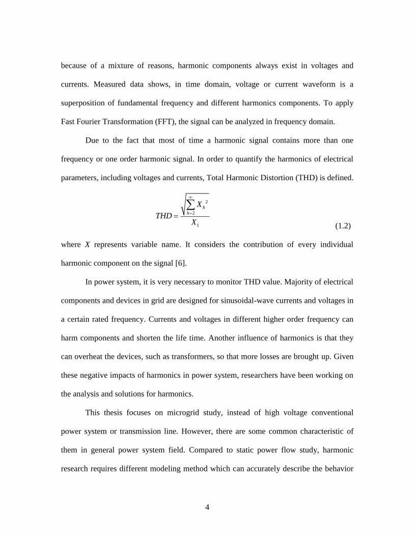
Due to the fact that most of time a harmonic signal contains more than one
frequency or one order harmonic signal. In order to quantify the harmonics of electrical
parameters, including voltages and currents, Total Harmonic Distortion (THD) is defined.
2
2
1
h
h
X
THDX
(1.2)
where X represents variable name. It considers the contribution of every individual
harmonic component on the signal [6].
In power system, it is very necessary to monitor THD value. Majority of electrical
components and devices in grid are designed for sinusoidal-wave currents and voltages in
a certain rated frequency. Currents and voltages in different higher order frequency can
harm components and shorten the life time. Another influence of harmonics is that they
can overheat the devices, such as transformers, so that more losses are brought up. Given
these negative impacts of harmonics in power system, researchers have been working on
the analysis and solutions for harmonics.
This thesis focuses on microgrid study, instead of high voltage conventional
power system or transmission line. However, there are some common characteristic of
them in general power system field. Compared to static power flow study, harmonic
research requires different modeling method which can accurately describe the behavior

5
of components in different frequencies. Simulation of the harmonic interaction between
detailed models of the synchronous generator, power transformer and transmission
system is achieved with the development of a unified multi-frequency domain equivalent
[7]. Also resonance phenomena could exist in transmission line because capacitors and
inductors have different reactance in higher frequency condition. Resonance happens
when the reactance of capacitor and inductor cancel out. In FFT harmonic spectrum, the
current near resonant frequency is much more dominant than those in other frequencies.
Because of the potential possibility of resonance, a seemingly small harmonic injection at
one location on the system causes significant problems some distance away such as
telephone interference [8].
There are several effective solutions for compensating harmonics in power system,
and among them active filters (AF) are highly focused by scholars: novel structures of
active filter can have lower voltage rating, smaller size inductor and lower
electromagnetic interference [9] [10]; with conventional concepts it takes one period of
fundamental frequency to eliminated the harmonics after the load current has changed but
newly built control scheme allows much faster harmonics reduction[11].
However, to design more suitable solutions for various conditions, it is important
to analyze the origins of harmonics in power system, which can be classified as two
major types: renewable energy and nonlinear loads. In this paper, only solar energy is
considered for renewable energy.

6
1.3 Photovoltaic Source
Photovoltaic (PV) is the technology that generates DC electrical power measured
in watts (W) or kilowatts (kW) from semiconductors when they are illuminated by
photons [12]. For the purpose of mathematically analyzing PV module and also
simulation work, a simplified model is shown in Figure 1.1.
IdRp
RsIout +
-
Vout
Ipv
Figure 1.1: Simplified PV Cell Circuit
Since the power of solar irradiance on the whole earth can be considered as
infinite for human beings, many scholars hold the opinion that PV is the solution to
energy crisis. Nowadays it is common to see solar panel (a set of PV cells) on residential
rooftops. They work very well on limited housing appliances, for example heating water.
Aiming to let solar energy replace more of conventional energy, utility-scale solar farm is
being studied and built increasingly. Besides PV panels, converters are used to regulate
DC voltage after the output of PV. Along with converters, Maximum Power Point
Tracking (MPPT) is one of the most important applications for PV source. Due to the
characteristic of PV cell researchers have developed various control scheme for MPPT to
provide the most power from PV cell when weather condition is given. If PV source is

7
connected with AC system, inverters are required to install after converters. Normally the
capacity of utility-scale solar farm is over 500 kW. In short duration of seven years, from
2004 to 2010, the total global grid-connected solar PV capacity has increased at an
average annual rate of 55%, to a total capacity of about 40 GW [13]. Even though this
new application has huge potential benefits, there are some technical concerns still
existing.
Previous work pertaining to solar PV applications in power systems can be
categorized into three major categories: modeling, technical impact, and financial
planning [14]. In this thesis, research focuses on the first two aspects. Various models
have been built and analyzed to study PV source’s impacts on power quality in
distribution systems [15-17]. One of the most important perspectives of power quality
study is harmonics analysis. In PV source, inverters are considered as sources of current
harmonics. Therefore, by improving control scheme of inverters, mitigation and
compensation of harmonics can be achieved [18, 19]. Also because of the intermittent
characteristic of solar irradiance, PV sources bring more uncertainty to systems. This
uncertainty includes time-varying penetration level and its impact on voltage profile [20]
and partial shading condition [21].
Large-scale PV source takes large areas. The limitation of PV farm size and
proper location for solar irradiance determine that instead of connecting to transmission
system directly, PV sources will have much more opportunities to serve microgrid. In the
fourth part of this chapter, the characteristic of microgrid is illustrated.

8
1.4 Nonlinear Load
Loads usually encountered in power systems can be broadly categorized into
industrial, residential, municipal and commercial loads [22]. When voltage and current in
same frequency have a linear relationship, this load can be called linear load. Most of
time, this type of loads is sets of linear resistors or linear inductors. However, different
from classic load theory, in reality there is no load is pure constant power or pure
constant impedance. So practical loads should be viewed as mixtures of linear loads and
nonlinear loads. Because of massive applications of power electronics, many electrical
devices are driven by multiple controllers or rectifiers. Different combinations of diodes
and capacitors can cause significant nonlinearity. For example, there is a battery charger
which is driven by a diode bridge rectifier (DBR) and if supplied by a pure sinusoidal AC
source of 110V the current waveform is shown in Figure 1.2.
Figure 1.2: Current Waveform of DBR
Thus how to model loads becomes a significant topic for power system research
in order to simulate systems accurately. Load models, regardless of the modeling

9
techniques, are divided into static and dynamic load models [23]. Static loads describe
the relationship between the power consumption, voltage and frequency [24], while
dynamic loads provide the additional advantage of representing time-sensitive behavior
of the load [25].
For static load modeling, there are two major theories: ZIP load model and
Crossed Frequency Admittance Matrix. The constant impedance, constant current, and
constant power components of a ZIP load are represented by a second-order polynomial
in bus voltage magnitude Vi [26]:
2
1 2 3( )Di i i i i i iP V a V a V a (1.3)
2
1 2 3( )Di i i i i i iQ V b V b V b (1.4)
where a1i, a2i, a3i, b1i, b2i and b3i are coefficients for power demand. The second order
term of voltage is for constant impedance (Z); the first order term of voltage stands for
constant current (I); and the zero order term of voltage is for constant power (P). This
method can give very accurate description of power consumption, voltage profile and
current flow. Nonetheless, it is not able to provide clear information of frequency
response of loads. Given the fact that harmonics study has crucial significance for power
quality, it is very necessary to consider a frequency dependent model for loads. Therefore
Crossed Frequency Admittance Matrix theory is suitable for harmonic model of loads.
This type of harmonic model takes into account the harmonic influence between
harmonic currents and harmonics voltages of different order. Equation (1.5) shows how
crossed frequency matrix represents this influence:

10
1 11 12 13 1 1
2 21 22 23 2 2
3 3
1
m
m
m m mm m
I Y Y Y Y V
I Y Y Y Y V
I V
I Y Y V
(1.5)
where voltages and currents are represented as complex numbers. The subscript m stands
for the harmonic order. For pure fundamental frequency voltage sources, voltage vector
elements are zeroes except V1. But currents flowing into loads still have harmonic
distortion due to the fact that Y21, Y31 and Ym1 are not all zeroes for nonlinear load. On
contrary, for linear load, the crossed frequency admittance matrix becomes a diagonal
matrix and the off diagonal elements are zeroes. The crossed frequency matrix models the
load as a harmonic currents source.
A proper load model is very important for doing case study in power system.
1.5 Microgrid Characteristics
Microgrid is a new concept which is brought up within the recent ten years. There
is no strict definition for microgrid, scholars share some same opinion about the
characteristics of microgrid.
It is running at low voltage level, mostly same voltage level as distribution
system. Microgrid concept assumes a cluster of loads and microsources as a single
controllable system that provides power to its local area [27]. Normally Microgrids are
considered as viable options for those places where main grid expansions is either
11
impossible or has no economic justification, such as the electrification in university
campuses, military installations and rural villages [1].
Conventional power systems have a configuration of one-way structure, which
means that there is only one source supplying the whole system. Therefore in
conventional power system, the power flow is only one-directional. But in microgrid,
these microsources can be installed in every possible locations, and it is also called
distributed generators (DGs). The types of DGs can be bio-mass generation, small-size
gas turbines, solar plant, wind plant and energy storage. The main purpose of microgrid is
to serve local area and finally reach to autonomous operation with less pollution. Based
on this purpose, sources of large capacity are not practical, instead small scale renewable
energy can play a key role.
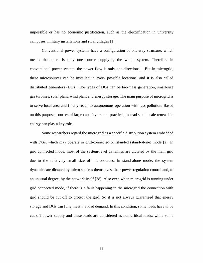
Some researchers regard the microgrid as a specific distribution system embedded
with DGs, which may operate in grid-connected or islanded (stand-alone) mode [2]. In
grid connected mode, most of the system-level dynamics are dictated by the main grid
due to the relatively small size of microsources; in stand-alone mode, the system
dynamics are dictated by micro sources themselves, their power regulation control and, to
an unusual degree, by the network itself [28]. Also even when microgrid is running under
grid connected mode, if there is a fault happening in the microgrid the connection with
grid should be cut off to protect the grid. So it is not always guaranteed that energy
storage and DGs can fully meet the load demand. In this condition, some loads have to be
cut off power supply and these loads are considered as non-critical loads; while some

12
loads have to maintain power supply for 24 hours and these loads are considered as
critical loads. Figure 1.3 shows a typical microgrid.
Grid
Substation
PCC
DGs
Battery
DGs
Noncritical
Load
Critical Load
Breaker
Figure 1.3: Typical Microgrid
Due to this special structure, along with this beneficial advantage, there are
potential challenges to keep the system running safe and well. One of main concerns in
the microgrid study is the electrical power quality issue.
Researchers have been doing works on how to monitor and simulate the actual
system. The first step of studying electrical power quality issues, particularly harmonics,
should be modeling a microgrid with renewable sources both in grid-connected mode and
stand-alone mode [15, 28, 29]. To address harmonics distortion, filters are designed and
tested by scholars. Compared to active power filters, passive filters consists of only
passive components and cost less. In [30] [31], several novel passive filters were
designed and tested to show the improvement. Yet passive filters can be very limited
when harmonic distortion is very serious and less predictable, since fixed passive filters
can only help decrease harmonics on the default setting orders. Thus, active power filters

13
were studied for harmonics issues in [11] [32]. Unfortunately, most of these researches,
which studied filter designs or inverter controls, were only focused on power electronic
fields regardless of the harmonics response in the microgrid.
According to previous researches, the factors which have influence on power
quality, specifically harmonics distortion, are very comprehensive. Therefore DGs,
inverters, weather conditions, energy storage and load modeling should be included all
together in the harmonics study in order to have better simulation results. Detailed study
is presented in the following chapters.
14
CHAPTER TWO
MODELLING OF MICROGRID
The study of microgrid can be achieved through different research methods,
including hardware test, computational programming, mathematical analysis and
software based simulation. As it is known that hardware test costs a lot and
computational programming is hard to describe the transient performance of some of
power electronic devices. In order to study the influence of harmonics in microgrid with
PV integration, software based simulation should be the best option. This thesis is based
on the results which come from computer simulations and therefore it is significant to
model each component in the microgrid in the most suitable ways. This chapter
demonstrates the details of modelling works of PV, nonlinear load, energy storage and
active power filter. Along with the process of modelling, the performances of each
components are also presented to prove the practicability.
2.1 Photovoltaic Source
2.1.1 Photovoltaic Source Modeling
In this thesis KC200GT is chosen as the model of PV cell used for integration.
The KC200GT data is determined by its own manufacture process. The data can be
obtained from the manufacturer data sheet and some parameters are shown in Table 2.1
[33].

15
TABLE 2.1
Parameters of KC200GT Solar Array at Nominal Operating Conditions
Imp 7.61A
Vmp 26.3V
Pmax,m 200.143W
Isc,n 8.21A
Voc 32.9V
I0,n 9.825 × 10⁻⁸ A
Ipv 8.241A
a 1.3
Rp 415.405 Ω
Rs 0.221 Ω
Kv -0.1230V/K
KI 0.0032A/K
The basic mathematical equation of PV array to describe I-V is shown below [34]:
( )
0[ 1]s out
t
V R I
V a
m pvI I I e
(2.1)
,[ ( )]pv pv n I n
n
GI I K T T
G (2.2)
,
,
0 ( )( )
( )
1
oc n v n
t
sc n I n
V K T T
aV
I K T TI
e
(2.3)
where Ipv is the current directly generated by one PV cell, I0 is the reverse saturation
current of the diode shown in Fig. 1.1, Im is the source current of PV cell, Iout is the

16
output current after resistance of PV cell, V is the output voltage, a is the diode ideality
constant, Vt is the thermal voltage of PV cell, Isc is the short circuit current of PV cell, T
is the temperature and G is the solar irradiance. Kv is the voltage gain of solar irradiance
and KI is the current gain of solar irradiance.
Based on the data in TABLE 2.1 and equation (2.1) to (2.3), mathematical model
was built in MATLAB/SIMULINK platform. After PV cell, a boost converter with
MPPT block was built. By comparing the output power and output voltage of PV cell on
very sample time period, PMW signal can be generated to gate of IGBT. And from there,
maximum power point can be traced. However, the output voltage of PV array itself is
not fit for the next level inverter control and a boost converter can improve the DC
voltage level. The structure is shown in Figure 2.1.
PV Array
L
MPPT
A
V C R
Boost Converter
Figure 2.1 Boost Converter with MPPT

17
2.1.2 Inverter Control of Photovoltaic Source
From previous researches there are two main methods for inverter control with
PV integration. One is Active Power Control (or called PQ control), and another one is
Voltage Frequency Control (or called VF control). When considering grid-connected
mode of microgrid, PQ control is the better option for lowering the reactive power output
from PV sources; when considering stand-alone mode operating, energy storage is the
slack bus in the system instead of PV so PQ control can help provide the most active
power for critical loads. Therefore, PQ control was built to be connected in PV source
system. Figure 2.2 shows the scheme of conventional configuration of three phase active
power inverter control. To be more specific, this control scheme has another name, feed-
forward decoupling PQ control. The dq transformation block can work as switching three
parameters (ia, ib, ic) of AC to two parameters (id, iq) in DC. The active and reactive
power signals (Pref, Qref) are used to obtain the reference signal (idref, iqref) of inner current
control loop by the matrix solver and equation (2.4) is given [35]:
( ) ( ) ( )( )
( ) ( ) ( )( )
d d dd
q q qq
i t u t e tR Li tdL
i t u t e tL Rdt i t
(2.4)
where L and R represent inductance and resistance of the impedance Za, Zb and Zc between
three phase inverter and voltage feedback in Figure 2.2. Since the purpose of this control
scheme is to force the reactive power output close to zero, the reference on q-axis set to
zero. The ud and uq are the output control signals of the current control block.

18
PV
Panel
Boost
Converter
with MPPT
Three Phase
Inverter Utility
abc dq
Pref, Qref
PWM
Current
Control Power
Control
idiq
iaib ic
idref
iqref
ed eq
ea
eb
ec
Za
Zb
Zc
Figure 2.2 PV System Including Inverter and Its Control Scheme
2.1.3 Simulation of Photovoltaic Source
Building PV source as a simulation file is aiming to help solve practical cases and
problems. In that way, it is necessary to prove the function and response of these
simulation blocks. The inputs of this PV cell are solar irradiance and temperature. In spite
of the fact that there are a lot of other parameters which can slightly influence the output,
for example humidity, solar irradiance and temperature are still the dominant factors over
all of others.

19
Figure 2.3: I-V Curve of Single PV Cell
under Different Solar Irradiances (at 25°C)
Figure 2.4: I-V Curve of Single PV Cell
under Different Temperatures (at 1000 W/m2)
0 5 10 15 20 25 30 350
2
4
6
8
10
Voltage (V)
Cu
rren
t (A
)
S=1000 W/m2
S=800 W/m2
S=600 W/m2
S=400 W/m2
S=200 W/m2
0 5 10 15 20 25 30 350
2
4
6
8
10
Voltage (V)
Cu
rren
t (A
)
T=50°C
T=30°C
T=20°C
T=10°C
T=0°C

20
Figure 2.5: P-V Curve of Single PV Cell
under Different Solar Irradiances (at 25°C)
Figure 2.6: P-V Curve of Single PV Cell
under Different Temperature (at 1000 W/m2)
0 5 10 15 20 25 30 350
50
100
150
200
250
300
Voltage (V)
Act
ive
Po
wer
(W
)
S=1000 W/m2
S=800 W/m2
S=600 W/m2
S=400 W/m2
S=200 W/m2
0 5 10 15 20 25 30 350
50
100
150
200
250
300
Voltage (V)
Acti
ve P
ow
er (
W)
T=50°C
T=30°C
T=20°C
T=10°C
T=0°C

21
From Figure 2.3 to Figure 2.6, curves are generated to prove the functions of PV
cell simulation block. In Figure 2.3, the I-V curves show that when boosting the voltage
after the maximum power point output currents drop quickly and higher irradiance can
generate higher current (nominal irradiance is 1000 W/m2). In Figure 2.4, the I-V curves
demonstrate that while boosting voltage after the maximum power point currents drop
quickly and lower temperature can slightly cause higher currents.
Figure 2.3 to 2.6 are based on the single PV cell simulation. However, a PV
source system consists of dozens of PV arrays which contains hundreds of PV cells. Here
in this thesis, each single PV source has 3000 PV cells to work together. At the nominal
condition which is at 25°C and 1000 W/m2, the rated output active power is 600 kW, also
shown in Figure 2.7. Furthermore, since the well-tuned inverter control can decrease the
harmonic distortion of output current, the simulation results in Figure 2.8 and 2.9 give
clear look at the output current at nominal condition when the voltage level is 4.16 kV.
Figure 2.7: Active Power Output of PV Source System at Nominal Condition
0 1 2 3 4 5 6 7 8 9 100
1
2
3
4
5
6
7x 10
5
Time (s)
Act
ive
Po
wer
(W
)

22
Figure 2.8: Output Current at Phase A of PV Source System at Nominal Condition
Figure 2.9: A Closer Look at
Output Current at Phase A of PV Source System at Nominal Condition
0 1 2 3 4 5 6 7 8 9 10-300
-250
-200
-150
-100
-50
0
50
100
150
Time (s)
Cu
rren
t (A
)
9.58 9.59 9.6 9.61 9.62 9.63 9.64 9.65 9.66 9.67
-100
-50
0
50
100
Time (s)
Cu
rren
t (A
)
23
2.2 Nonlinear Composite Load
2.2.1 Nonlinear Load Modeling Method
Many theories have been proposed for nonlinear load modeling but as it is
mentioned in Chapter II Crossed Frequency Matrix can demonstrate the harmonic
response of different types of loads. Therefore, in this study Crossed Frequency Matrix is
applied to model the load. Particularly, instead of only modeling one type of load, here a
composite load is aiming to be modeled. For the purpose of composite load simulation,
with given voltages, output currents can be monitored. When monitoring output currents,
time domain current waveform is analyzed by the Fast Fourier Transformation (FFT) so
that it can be expressed as a complex number matrix. In this complex matrix, each row
stands for a current on a distinct harmonic order. In microgrid, other than resonance
phenomenon, high frequency harmonic currents have quite small magnitude. It is not
practical to consider every order of harmonic currents that exist in the system. In order to
simplify the modeling process, here the complex matrix only includes from fundamental
current up to 13th order of harmonic current. With only fundamental voltage, 60 Hz, first
column elements in crossed frequency admittance matrix can be calculated. Then by
superimposing 3rd, 5th, 7th, 9th, 11th and 13th order harmonic voltage sources, each one at a
time, the other columns can be calculated likewise. Therefore, three 7×7 admittance
matrixes are built for the three types of nonlinear loads. Equation (2.5) demonstrates how
each harmonic order current is determined through the Crossed Frequency Matrix which
is shown in equation (1.5) and m, n both represent harmonic order number. And equation
(2.6) and (2.7) explain how elements in the matrix is calculated.

24
𝐼1 = 𝑌11 𝑉1 + 𝑌12
𝑉2 + 𝑌13 𝑉3 + ⋯ + 𝑌1𝑛
𝑉
𝐼2 = 𝑌21 𝑉1 + 𝑌22
𝑉2 + 𝑌23 𝑉3 + ⋯ + 𝑌2𝑛
𝑉
… …
𝐼 = 𝑌𝑚1 𝑉1 + 𝑌𝑚2
𝑉2 + 𝑌𝑚3 𝑉3 + ⋯ + 𝑌𝑚𝑛
𝑉 (2.5)
(2.6)
(2.7)
2.2.2 Individual Nonlinear Load Types
• Instead of making the assumption of single type load, in order to consider the
practical situation of microgrid load demand, in this study a composite load is modeled,
including three types of nonlinear load and one linear load. The first nonlinear load type
is compact fluorescent light (CFL), which is the basic load in residential systems. Then
the second one is load with diode bridge rectifier (DBR), which is widely applied to a
large amount of home appliances including desktop computers, television sets, battery
chargers, adjustable speed drives for heating pumps and air conditioning etc. The third
type is load with phase angle AC voltage controller (PAVC), which normally used in
light dimmers, heating load, single-phase induction motors. The structure of this
composite load is shown in Figure 2.10.
𝑌𝑘1 =
𝐼
𝑉
𝑌𝑘𝑗 =
𝐼𝑘−𝑌𝑘1𝑉1
𝑉𝑗

25
Figure 2.10: Composite Load Structure
The next step is to use simplified circuit to represent each type of load and
calculate each admittance matrix according to equation (2.6) and (2.7). In Figure 2.11,
each type of nonlinear load simplified circuit is given. First, to connect an AC source
with only fundamental frequency to each circuit and then from simulation results currents
can be recorded and divided into each frequency by FFT. From equation (2.6), elements
in the first column can be found. Secondly, to superimpose one j order harmonic voltage
source to the previous circuit and elements on column j can be calculated by equation
(2.7).

26
AC R
C1
C2
AC R
AC R
DBR
CFL
PAVC
Linear
(a) (b)
(c) (d)
Figure 2.11: Simplified Circuit of Composite Load: (a) CFL; (b) DBR;
(c) PAVC; (d) Structure
Figure 2.12 shows the simulation of a 15W CFL load, which is under 120V AC
voltage level. According to the results of current FFT, the Crossed Frequency Admittance
Matrix is calculated (the matrix is provided in Appendix A). In Figure 2.13, the value of
Z axis shows the magnitudes of each elements in the admittance matrix while X and Y
stand for the harmonic orders. Obviously, this load is far away from being linear and 5th,
7th, 11th harmonics are the main factors.

27
Figure 2.12: Simulation of CFL
Figure 2.13: Admittance Matrix Magnitude Distribution of CFL

28
Similarly, Figure 2.14 shows the simulation of 0.67 kW DBR and Figure 2.15
gives the demonstration of the magnitudes of elements in this matrix. Compared to the
matrix of CFL, this one has different characteristic. Diagonal elements have the largest
magnitude and this can be interpreted that there is relatively small interaction between
different frequencies. Meanwhile, among diagonal elements, ones which represent for
11th and 13th order harmonic frequencies have larger magnitudes, which means that on
high frequency this load has smaller resistance.
Figure 2.14: Simulation of DBR

29
Figure 2.15: Admittance Matrix Magnitude Distribution of DBR
A 0.9 kW PAVC type load is simulated as Figure 2.16. Figure 2.17 shows that a
load with PAVC can be close to linear load, since there is fairly small interaction between
frequencies and magnitudes of diagonal terms are almost the same.
Figure 2.16: Simulation of PAVC

30
Figure 2.17: Admittance Matrix Magnitude Distribution of PAVC
2.2.3 Simulation Model Building
After obtaining the crossed frequency admittance matrix for each type of
nonlinear load, the next goal is to include these matrices into simulation. Assuming the
total load demand is fixed, and with the same amount of active power and power factor
the numbers of each type of loads which were described above can be estimated. In real
residential system, most of house appliances are connected in parallel so that individual
equipment can work independently. Thus, total current will simply be sum of the
individual currents. And different loads contain nonlinear loads with different ratios.
Figure 2.18 explains how this mathematical model works in the simulation of microgrid.
Firstly, voltage measurement unit is able to obtain voltage information from the feeder in
microgrid. And then through Fourier transformation, signals in time domain can be

31
transformed into frequency domain and be formed into a voltage matrix. This voltage
matrix has only one column complex numbers and each row represents one harmonic
order. According to equation (2.5), with both admittance matrix and voltage matrix, the
current matrix can be calculated. Therefore, using the complex number in current matrix,
a current signal in time domain can be generated to control the controllable current source
to draw currents from the feeder. Along with the process of nonlinear load, linear load is
also connected in parallel.
Voltage
Measurement
Fourier
Analysis
Va
Magnitude
Phase Angle
Generate Voltage
Matrix
Admittance Matrix of
Nonlinear Load
Multipli-
cationCurrent
MatrixMagnitude
Phase Angle
Current
Waveform
Feeder in Microgrid
Controllable
Current Source
Linear Load
Inonlinear
Ilinear
Figure 2.18: Composite Load Simulation Scheme Diagram

32
2.3 Energy Storage
Energy storage is one of the most unique part of microgrid structure. Because
microgrid should be able to operate either under grid-connected mode or stand-alone
mode, energy storage is necessary for stand-alone operating. In stand-alone mode, the
most important requirement is to provide reliable power to customers. However,
renewable energy, such as PV source, has intermittent characteristic and weather
dependent restrictions. Particularly solar irradiance varies during daytime so that the
output of PV source varies greatly with irradiance. Thus, other stable types of distributed
sources are necessary in a microgrid. In most practical applications, batteries and diesel
generators, which work as the slack bus in stand-alone mode, can supply stable voltage
and frequency for the system.
Beside PQ control, v/f control and droop control are often used in inverter control
of distributed sources in microgrid. Since the goal of PQ control is to achieve the
maximum output of active power and minimum reactive power, it is used for PV control
in grid-connected mode and stand-alone mode. However, in stand-alone mode, energy
storage bus should be the slack bus. Slack bus works to provide stable voltage and
frequency for the system, therefore v/f control and droop control are often used for
inverter control of battery. Compared to v/f control, droop control does not maintain the
same stable voltage and frequency but varies in a small range with the output. Higher
active power output can causes small drop on frequency and higher reactive power output
can cause small drop on voltage.

33
( )ref x reff f k P P (2.8)
( )ref y refV V k Q Q (2.9)
However, because of this characteristic, multiple batteries and other type of
microsources can work together to communicate. So in this study, droop control is
appliced to the inverter control of the energy storage, which is a DC battery. The control
scheme and structure is shown in Figure 2.19. Furthermore, the performance of this
simulation model is going to be shown and explained in the next chapter.
3-phase
Output
Voltage Signal
3-phase Output
Current Signal
Power
Calculation &
abc/dq
Transformation
Output
Active
Power
Output Reactive
Power
Current &
Voltage in dq
axises
Pref Qref
Minus
fref Vref
Sum
Minus
kx
ky Minus
Vref in
dq
axises
PID Controller
& dq/abc
Transformatio
n
PWM
Generator
PWM signal
to inverter
Figure 2.19: Droop Control Structure of Storage Battery

34
2.4 Active Power Filter
The design of active power filter is not the focus point of this research. Yet, when
discussing harmonics distortion problem, the solution is always about filter design and
installation. In a multi-battery microgrid, harmonics can be much higher in stand-alone
mode than in grid-connected mode. Sometimes, too much harmonics can have quite
negative influence on power devices and customers. Thus, a proper designed filter should
be considered as an important part of microgrid system.
2.4.1 Structure of Active Power Filter
Harmonics can cause damages on electrical devices, such as, overheating
transformers. Therefore, it is very important to monitor power quality in the grid,
especially harmonic distortion levels. If harmonic distortion is beyond the regulation, it is
necessary to install filters to mitigate harmonics. There are two types of filters in general:
passive filters and active power filters.
Renewable energy inverters are the main source of harmonics, the magnitudes of
current on each harmonic are changing all the time along with weather conditions, such as
solar irradiance. However, passive filters are set to decrease the current magnitude in some
specific harmonic order. If these magnitudes are changing, it is hard to choose which
frequency to be tuned to improve the power quality significantly because the major
harmonics distortion might not be the one from the initial design. Thus, an active power
filter can help improve power quality by having an active power source with controllers,
shown in Figure 2.20 [9].

35
Zl
Zl
Zl
Active Power
Filter
Nonlinear
LoadGrid
Three-Phase
Inverter
Feeder
Figure 2.20: Active Power Filter Structure
2.4.2 Simulation of Active Power Filter
In order to show the performance of the active power filter mentioned above, a simple
simulation study was done. The presented parallel three phase inverter can be controlled
by different types of control schemes and the advantages and disadvantages are discussed
in [36]. The proposed model is using a current compensation method, called Instantaneous
Reactive-Power algorithm [37]. When the active power filter is connected to the grid, the
power delivered on different frequencies can be calculated. By a basic 5th order
Butterworth low pass filter, power that is delivered on high frequency can be detected and
be considered for compensation control scheme. Therefore, the inverter can control the
filter to compensate current harmonics through PWM signals, not only in one specific
order but more generally. To test this active power filter simulation model, it is connected
with a nonlinear load on 4.16 kV (phase to phase) voltage source. From current

36
waveforms shown in Figure 2.21, it can be observed that the harmonics distortion is
improved significantly. By FFT, the current magnitude spectrum on frequencies is
presented as follows. Figure 2.22 gives the FFT spectrum of source current without active
power filter while Figure 2.23 shows the spectrum after the filter is connected. From the
comparison between Figure 2.22 and Figure 2.23, Total Harmonic Distortion (THD) drops
from 19.70% to 3.42% and harmonics on 5th order drops from 15% to 0.35%.
Figure 2.21: Current Waveform (at 0.2s the active power filter is connected)
Figure 2.22: FFT Spectrum of Source Current without Active Power Filter
-100
0
100
-100
0
100
Curr
ent
(A)
0.19 0.2 0.21 0.22 0.23 0.24-100
0
100
Time (s)
Current (A)
0 2 4 6 8 10 12 14 160
5
10
15
Harmonic order
Fundamental (60Hz) = 89.17 , THD= 19.70%
Ma
g (
% o
f F
un
da
men
tal)

37
Figure 2.23: FFT Spectrum of Source Current with Active Power Filter
2.5 Summary
This chapter includes simulation modelling works for each component in this
microgrid study. Specifically the structure of microgrid consists of renewable source,
nonlinear load, energy storage and potential power filter. Traditional simplified model or
equations which describe the relation of input and output cannot meet the requirement of
harmonics study since it mainly supports steady state study. Steady-state study only gives
the values and information of steady state output or parameters in the power system
without considering short-time transient conditions. Nevertheless, the origins of
harmonics are from inverter performance in transient status. For a long time this area
studies have been regarded as the focus area for scholars who major in Power
Electronics. Consequently researches in Power System area have ignored the detailed
model of various types of inverters while dealing with microgrid. Therefore what makes
this chapter important is while studying the harmonics influence of microgrid, the
0 2 4 6 8 10 12 14 160
0.1
0.2
0.3
0.4
Harmonic order
Fundamental (60Hz) = 89.22 , THD= 3.42%
Ma
g (
% o
f F
un
da
men
tal)

38
detailed models are not ingored so that the simulation can give more practical
demonstration. Especially loads and sources, which are major origins of current
harmonics in microgrid, are well modelled from the view of harmonics. With the detailed
models built in this chapter, more simulations results can be persuasive and solid.

39
CHAPTER THREE
HARMONICS IMPACTS ON MICROGRID
The research method of this thesis study is to use computer software to simulate
the influence brought by PV integration in microgrid. Based on the modelling work
mentioned in Chapter 2, multiple simulations can be conducted to analyze harmonic
distortion influence. Specifically, both grid-connected and stand-alone mode are studied.
In order to evaluate harmonics with quantified indices, several power quality indices are
described in the following part.
3.1 Power Quality Indices
Power quality indices are parameters that are able to show some part of electric
characteristic according to current or voltage measurements. In other words, power
quality indices are defined to quantify the distortion for current or voltage. Each index
has different function to describe the distortion. Therefore, multiple indices should help
researchers to have a clear look at the harmonics distortion from various perspectives.
THD is the measurement of the harmonic distortion at each node on each bus in
the system. In order to look at the harmonic distortion in the whole system, whole system
harmonics distortion level (WSHDL) is defined as:
n
THDWSHDL
n
i i 1 (3.1)
where n is the number of nodes; h represents the harmonic order; m is the considered

40
maximum harmonic order. I1 is the absolute value of fundamental (60Hz) current. The
meaning of this definition is to have a great picture for the harmonics distortion trend.
Also in low voltage level system, such as microgrid or distribution systems, instead of all
three-phase line structure, there are many two-phase feeders or single-phase feeders.
Therefore, it is important to look into each node on each bus.
In addition to the WSHDL, there are three types of PQ indices are introduced and
discussed along with simulation results. Distortion power DP index is defined in (3.2)
[38]. The total apparent power, fundamental active power and fundamental reactive
power are defined in (3.3) to (3.5).
2 2 2 2 2 2
1 1 1 1 ( )V I V IDP S P Q V I THD THD THD THD
(3.2)
where the total apparent power 1 1
2 2
0 0
( ) ( ) ,m m
n n
S V n I n
(3.3)
fundamental active power 1 1 1 cos( ),P V I (3.4)
fundamental reactive power 1 1 1 sin( )Q V I (3.5)
By normalizing DP to unity, normalized DPnorm index can be obtained. DP index
has the ability to show contributions of distortion power from individual customers to
PCC. From (3.2), it is easy to estimate the power delivered not on 60 Hz simply by taking
measurements of THD into the equation. This index is crucial for utility to monitor how
much power is lost. Waveform distortion WD index is defined as [39]:

41
2 2 2
1 1 int , int , 1
2 1
/ IM N
m eg h i er h j
i j
WD I I I I
(3.6)
where I1 is the rated current magnitude and Im1 is the measured fundamental current
magnitude. Iinteg-h,i is the ith integer harmonic component and Iinter-h,j is the jth inter-
harmonic component. WD index expresses how much a component, AC current, is
distorted or deviated from ideal sinusoidal waveform. WD index includes inter-harmonic
components, which can take a large part of harmonics when different types of inverters
involved. Also inter-harmonics cannot be presented by THD which only include integer
order of harmonics. Instead of an average value, WD index gives an instantaneous
distortion ratio and it can be depicted along with time axis to be monitored. Symmetrical
components deviation SCD index is defined as [38]:
2
2 2
1 1/ Imp mn mzSCD I I I I
(3.7)
where Imp, Imn, Imz are the measured currents at positive, negative and zero sequences.
SCD index has a significant meaning for microgrid because it can give the level of
unbalance on currents. SCD index can help staff who work in substations to recognize the
unbalance in each node and its impact on the whole system.
3.2 Test System Information
Study system shown in Figure 3.1 is a 14-bus 4.16 kV microgrid (located in GA,
USA). The detailed feeder configuration and its impedance matrices are presented in

42
Appendix B. Bus 10 is the slack bus and the balance point in grid-connected mode. The
slack bus voltage is set to 1.05 pu to keep all node voltages at least 0.95 pu. In Figure 3.1,
three lines represent three phase feeder. Two lines represent two phase feeder and single
line means one phase feeder. Load information is given in Table 3.1. The PV sources as
the only type of renewable energy are integrated to the system as shown in Figure 3.1.
The inverter control inputs ea, eb, ec, ia, ib, ic are obtained from monitoring the integration
point in microgrid. If these values are away from ideal balanced condition and changing
along with time, then PV sources will provide more harmonics than running under ideal
balanced condition because of the performance of inverters. Figure 3.2 shows the solar
irradiance and temperature during 24 hours (average value of typical day of July within
10 years). Since in the simulation model, PV’s output is only influenced by temperature
and solar irradiance, only these two factors are considered in the typical day of July. In
this work, the simulation only runs during the sunniest period (7am to 6pm).
Bus 10
Bus 20
Bus 30
Bus 31
Bus 32 Bus 33
Bus 34
Bus 40
Bus 50
Bus 60
Bus 61
Bus 41
Bus 62
Bus 51
GridPV
PCC
Figure 3.1 Test System Structure

43
Table 3.1 Load Data of the Study System
Bus
Load Data for the System
Note Active
Power (kW)
Reactive
Power
(kVar)
10 — — —
20 Three phase 630 212
30 Three phase 412 112
31 — — —
32 One phase 37 12
33 One phase 24 8
34 Three phase 343 122
40 Three phase 175 100
41 Three phase 133 51
50 Three phase 298 151
51 Two phase 68 12
60 Three phase 200 70
61 Three phase 74 28
62 One Phase 32 11
0 5:00 10:00 15:00 20:000
100
200
300
400
500
600
700
800A Typical Day of July
Time (hour)
so
lar i
rrad
ian
ce (
w/m
2)
0:00 1:00 2:00 3:00 4:00 5:00 6:00 7:00 8:00 9:00 10:00 11:00 12:00 13:00 14:00 15:00 16:00 17:00 18:00 19:00 20:00 21:00 22:00 23:00 24:00
21
23
25
27
29
31
33
35
Time (hour)
tem
peratu
re (
°C
)
Figure 3.2 Meteorological Data on Typical July Day

44
3.3 Harmonics Impacts on Grid Connected Mode
The test system is simulated in this section in MATLAB/Simulink and analyzed
considering the PV model and the composite load model explained in 2 to study the
harmonic distortion and PQ indices described in section 3.1. The PV data are set as in
Table 3.1. After running the power flow in the basic microgrid (without PV integration
and without nonlinear loads), voltages on each node are found in the acceptable
fluctuation range (0.95, 1.05 pu).
3.3.1 Considering PV with Linear Load
Two cases are studied based on PV locations. In case I, PV locations shown in
Figure 3.1 are considered. Applying equation (3.1) gives the harmonics distortion data for
each bus from 7:00 am to 6:00 pm. WSHDL values demonstrates the harmonics
distortion in the microgrid system as shown in Figure 3.3. In Figure 3.3, the harmonic
distortion is significant at noon time. In other words, as the percentage of power supplied
by PV is going higher, the WSHDL is going higher. This phenomenon can be explained
by the fact that inverter produces harmonics and more power coming from PV means
more distorted power is generated. THD provides analysis in each bus as shown in
Figure 3.4. According to the standards in [40], when voltage level is under 69 kV and
Isc/IL is smaller than 20, THD of current is regulated under 5% by standards. So the THD
values above 5% represent nodes that largely influenced by PV integration and some
potential damage might be caused by harmonics to shorten the lifetime of electrical
components.

45
7:00 8:00 9:00 10:00 11:00 12:00 13:00 14:00 15:00 16:00 17:00 18:000
0.2
0.4
0.6
0.8
1.0
1.2
1.4
1.6
1.8
2.0
2.2
2.4
Whole System Harmonics Distortion Level
time (hour)
percen
t %
Injection at Bus 50 60 & 61
Figure 3.3 WSHDL from 7:00AM-6:00PM (Case I)
7:00 8:00 9:00 10:00 11:00 12:00 13:00 14:00 15:00 16:00 17:00 18:000
5
10
15THD Plots of Case I
Ha
rm
on
ics D
isto
rti
on
(p
ercen
tage%
)
Time (hours)
20A
30A
34A
40A
41A
50A
60A
61A
32
33
51A
51B
62
5% harmonics is the
regulated limit
Figure 3.4 THD from 7:00AM-6:00PM (Case I)

46
In case II, the PV sources are integrated at buses 20, 40 and 60. Figure 3.5 shows
the WSHDL of case II. In Figure 3.6, the red line (phase A of bus 50) is the most
affected. However, THD value on all these nodes are under 5%, which is acceptable for
microgrid system. Compared to case I, the integration locations affect the THD. In case I
WSHDL is large when the penetration level is high; however in case II WSHDL is not
affected much by the penetration level change. This results give a clear demonstration
about how the integrations of PV affect the microgrid distortion. However, when THD is
over 5% the power quality is required to be improved.
7:00 8:00 9:00 10:00 11:00 12:00 13:00 14:00 15:00 16:00 17:00 18:000
0.05
0.10
0.15
0.20
0.25
0.30
0.35Whole System Harmonics Distortion Level
time (hour)
percen
t %
Injection at Bus 20 40 & 60
Figure 3.5 WSHDL from 7:00AM-6:00PM (Case II)

47
7:00 8:00 9:00 10:00 11:00 12:00 13:00 14:00 15:00 16:00 17:00 18:000
0.5
1.0
1.5
2.0
2.5
3.0
3.5
4.0
THD Plots of Case IIH
arm
on
ics D
istortio
n (
percen
tage%
)
Time (hours)
20A
30A
34A
40A
41A
50A
60A
61A
32
33
51A
51B
62
Figure 3.6 THD from 7:00AM-6:00PM (Case II)
Compared to the case I, the integration locations in case II are more dispersed on
this radial system. According to the theory of PQ control inverter which is introduced in
Chapter 2, since each PV source are separated and slack bus can provide nearly ideal
balanced power from the grid side in grid-connected mode, the inverter PQ control
should be improved by less distortion reference currents and voltages. Figure 3.3 and
Figure 3.5 give a clear presentation of the difference between two location choices for
three PV sources.

48
3.3.2 Considering PV with Nonlinear Composite Load
This part investigates the effect of nonlinear loads. According to experiences from
Grainger Industrial Supply [41], a normal business building can withstand up to 15% of
nonlinear load without apparent negative influences. But when it comes larger than 15%,
necessary devices should be installed to improve power quality. Nonlinear loads are
added at different percentage w.r.to the linear loads. Blue solid line in Figure 3.7 shows
the current waveform with 10% of nonlinear load at Bus 61, phase A. At this time, the
THD is 4.0% as shown in Figure 3.8. Red solid line in Figure 3.7 represents the 15% of
nonlinear load at the same node and the corresponding THD is 5.6%. Figure 3.8 shows
how the current harmonic distortion increase with increasing the percentage of nonlinear
load. The nonlinear load is the same as the one mentioned in Chapter 2 and each type of
the admittance matrix is presented in Appendix A.
0.26 0.27 0.28 0.29 0.3 0.31
-15
-10
-5
0
5
10
15
Time (s)
Cu
rren
t (A
)
Comparison
with 10% nonlinear
with 15% nonlinear
Figure 3.7 Load Current of Bus 61A with Nonlinear Load

49
0 5% 10% 15% 20%0
1%
2%
3%
4%
5%
6%
7%
8%
Nonlinear Proportion
TH
D
Regulated Limit
Figure 3.8 THD Comparison with Different Loads with PV Injection
Substation
PV
3 Phase3 PhaseTwo Phase Single
Phase
Bus 62
Residential
Building
Bus 60
Business
Building
Bus 61
Business
Building
Bus 51
Small Factory
AC
DC
PCC
Figure 3.9 Simplified Study System

50
For the purpose of PQ indices investigation, the microgrid system in Figure 3.1 is
simplified as shown in Figure 3.9. An equivalent PV source is considered at the PCC
point. The simplified system consists of four main loads. The composite load information
is shown in Table 3.2. Bus 51 (considered as a small scale factory and because of large
amount of motors and heating pumps) is a PAVC type of nonlinear loads. Buses 60 and
61 (two business buildings which contain many devices like computers) are classified as
DBR. Load of bus 62 is considered residential. PQ indices in section 3.1 are applied on
the simplified system. Harmonics distortion ranking (HDR) can be found through
descending sorting of DP and WD indices. The simulation results are shown in Tables 3.3
and 3.4. All these results are based on currents measurement because voltage distortion is
not dominant compared with currents. Table 3.3 lists the DP index which implies that the
large amount of load contributing more to DP and the ranking gives the same
information. However in Table 3.4, the WD index reflects that without considering power
but the waveform of currents. Clearly, due to large use of motors, heating pumps and
other heavy duty nonlinear loads, even load on Bus 51 does not consume the most power
but it still has the worst impact on current waveform. In Table 3.4, the HDR is different
with that in Table 3.3; this can give substation engineers multiple views of power quality.
The SCD index can indicate how much unbalance the system have from data obtained at
PCC. But before applying the SCD equation, one assumption has to be made that in this
case study mutual coupling between lines can be neglected due to the short length of each
feeder. According to simulation results, the magnitude of current sequences running
through PCC is [25.87 12.64 10.23] Amps ([positive negative zero]). By applying

51
equation (3.7), the SCD index is 0.54. SCD index could weight from 0 to 1 and larger
number shows more unbalanced. The contribution of harmonics from PV inverter,
different types of nonlinear loads on each phase and system configuration have
determined that this microgrid is very unbalanced. Engineers who work in substations
can also use SCD as power quality index for regulating the system.
Table 3.2 Composite Load Information
Bus Number Phase DBR CFL PAVC Linear Load
51 A&B 15% 15% 30% 40%
60 ABC 20% 20% 10% 50%
61 ABC 25% 25% 10% 40%
62 C 15% 10% 15% 60%
Table 3.3 Distortion Power Index
Bus
Number Phase DPnorm HDR
51 A 0.0791 7
51 B 0.0787 8
60 A 0.1417 3
60 B 0.1798 1
60 C 0.1645 2
61 A 0.0793 6
61 B 0.1072 4
61 C 0.0977 5
62 C 0.0720 9
52
Table 3.4 Waveform Distortion Index
Bus
Number Phase WD HDR
51 A 0.482 2
51 B 0.511 1
60 A 0.301 9
60 B 0.336 7
60 C 0.324 8
61 A 0.382 6
61 B 0.453 3
61 C 0.419 5
62 C 0.437 4
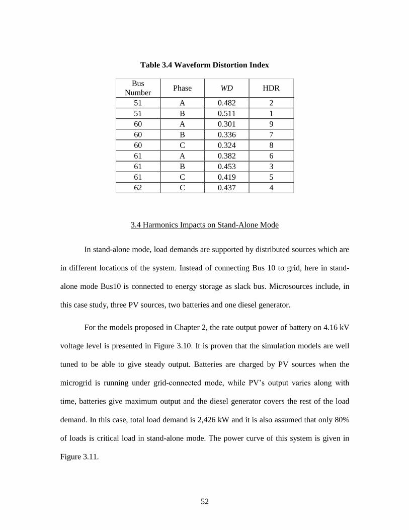
3.4 Harmonics Impacts on Stand-Alone Mode
In stand-alone mode, load demands are supported by distributed sources which are
in different locations of the system. Instead of connecting Bus 10 to grid, here in stand-
alone mode Bus10 is connected to energy storage as slack bus. Microsources include, in
this case study, three PV sources, two batteries and one diesel generator.
For the models proposed in Chapter 2, the rate output power of battery on 4.16 kV
voltage level is presented in Figure 3.10. It is proven that the simulation models are well
tuned to be able to give steady output. Batteries are charged by PV sources when the
microgrid is running under grid-connected mode, while PV’s output varies along with
time, batteries give maximum output and the diesel generator covers the rest of the load
demand. In this case, total load demand is 2,426 kW and it is also assumed that only 80%
of loads is critical load in stand-alone mode. The power curve of this system is given in
Figure 3.11.

53
Figure 3.10 Battery Rated Output Active Power
Figure 3.11 Active Power Curve of Microgrid in Stand-alone Mode
0 0.4 0.80
0.5
1
1.5
2
2.5
3x 10
5
Time (s)
Act
ive
Po
wer
(W
)
7 8 9 10 11 12 13 14 15 16 17 180
200
400
600
800
1000
1200
1400
Time (hour)
Act
ive
Po
wer
(k
W)
Battery
PV Source
Diesel Generator

54
Both nonlinear loads and inverters generate harmonics and the harmonic
distortion is able to influence the output current of energy storage. Figure 3.12
demonstrates how THD of battery output current changes during the day from 7:00 AM
to 6:00 PM. In Figure 3.12, the red line stands for THD values without active power filter
while the green line stands for THD values with active power filter. Without filter,
harmonics value can be higher than 5%, which can potentially harm the transformer
located between the battery and the microgrid. Even when the nonlinearity ratio of load
increases, this THD value could be much higher. After being connected with the active
power filter, the THD values are largely decreased. In this case, the highest value of THD
is not over 1%. Though active power filter can work effectively, it is not practical to
install many active power filters in one microgrid considering the cost. Installing one
active filter on the slack bus to protect energy storage is practical since the initial cost of
battery and larger size transformer are more expensive.
Figure 3.12 THD of Battery Current Output from 7:00AM to 6:00PM
7 8 9 10 11 12 13 14 15 16 17 181
1.5
2
2.5
3
3.5
4
4.5
5
5.5
6
Time (h)
TH
D in
Percen
tag
e
7 8 9 10 11 12 13 14 15 16 17 180
0.2
0.4
0.6
0.8
1
TH
D i
n P
ercen
tag
e
wtih filter
without filter

55
In Figure 3.13, WSHDL is plotted from 7:00 AM to 6:00 PM. While the solar
irradiance is increasing along with time, the increase of WSHDL means that the harmonic
distortion gets worse. For a grid-connected system, if the value of WSHDL is above 1%,
that means some of nodes are suffering from significant harmonic distortion. Because
when system is running under grid-connected mode THD near PCC is very small if
assuming the grid does not deliver much harmonics, there must be some buses which
suffer from high THD. Nevertheless, in Figure 3.13, it is easy to notice that WSHDL is
keeping above 2%. This can be viewed as one of the major difference between grid-
connected mode and stand-alone mode. Since the slack bus in stand-alone mode is the
one which is connected with the energy storage and generators, there are always a certain
amount of high frequency currents from the slack bus. If the nonlinearity of load becomes
more significant, it is even harder to keep THD lower than 5% on each node. When the
average THD of each node is 5%, WSHDL is 2.236%. Figure 3.14 presents THD on each
node along the same time period.
According to the comparison between Figure 3.13 and Figure 3.14, WSHDL has
the advantage of showing the trend of the whole system with one simple parameter based
on THD values. Without looking into every line in Figure 3.14, how the harmonics
distortion varies in the whole microgrid can be found in Figure 3.13. However, THD
plots provides a more accurate close look at each current, which can be analyzed
individually.

56
Figure 3.13 WSHDL of Study System from 7:00AM to 6:00PM in Stand-alone Mode
Figure 3.14 THD of Study System from 7:00AM to 6:00PM in Stand-alone Mode
7 8 9 10 11 12 13 14 15 16 17 180
0.5
1
1.5
2
2.5
3
3.5
Time (hour)
Percen
t %
7 8 9 10 11 12 13 14 15 16 17 180
2
4
6
8
10
12
Ha
rm
on
ics D
isto
rti
on
(p
ercen
tag
e%
)
Time (hours)
Bus 20
Bus 30
Bus 34
Bus 40
Bus 41
Bus 50
Bus 60
Bus 61
Bus 32
Bus 33
Bus 51a
Bus 51b
Bus 62
57
3.5 Summary
This chapter discussed the impact of two harmonic sources: PV sources and
nonlinear load, in a microgrid in both grid-connected mode and stand-alone mode. Firstly
the PV source integration is studied using linear loads; then PV sources are combined
with nonlinear loads. While considering only linear loads, this study provides a
comparison between two types of PV integrating locations. Then the whole system
harmonics distortion level as well as the THD are considered as the main measures to
evaluate the power quality and impact of PV integrations. Instead of single PV source,
this study investigates mutual influences with multiple PV sources. An actual microgrid
with historical-based weather conditions is used as a study system. Simulation results can
indicate a discernible look at these negative impacts on the microgrid power quality. In
order to make numerical comparison and ranking power quality indices are used to
estimate the current distortion from several different perspectives. Three PQ indices are
applied and compared to investigate the power distortion, waveform distortion and
system unbalance. And using the same models that were applied in grid-connected mode
study, stand-alone mode was investigated mainly by THD and WSHDL. Because the
slack bus in stand-alone mode is the energy storage battery and diesel generators, it
cannot provide power of the same quality as from the grid side. From multiple figures,
the microgrid suffers much more from harmonics distortion in stand-alone mode.
Simulation models and used matlab codes are shown in Appendix C.

58
CHAPTER FOUR
CONCLUSION AND FUTURE WORK
The initial motivation of this thesis study is from the special structure of
microgrid which might be the future solution of power delivery. As it has been presented
above, microgrid is a low-voltage power system with small size capacity and complicated
feeder configuration. While analyzing the whole microgrid system, different with
simplified mathematical model, detailed models are able to present better view on
monitoring and assessment of harmonics. An accurate harmonics study can help reduce
power loss, financial loss and operating stability of microgrid.
Given the fact that microgrid is aiming to serve local area, it becomes one of the
most promising application platform of renewable energy. Specifically in this thesis, PV
integration is analyzed. The major issue of the PV integration is harmonics distortion
which is the focus point in this research.
In Chapter One, some related basic background knowledge were presented as the
foundation of the research. In addition, previous works by other scholars were mentioned
as literature review to give a clear picture of what has been accomplished and what need
to be improved. These foundation explains the significance of electrical power system
harmonic study, what is microgrid and why it is different from conventional distribution
system. In Chapter Two, the main content is that how the components in microgrid are
modelled for simulation. PV cell and nonlinear loads were modelled from mathematical

59
equations while inverter control schemes in both PV system and energy storage were
achieved through control blocks in Matlab/Simulink platform. Mathematical equations
express the relationship between input and output, mostly in steady state condition.
However, the Crossed Frequency Admittance Matrix is able to describe the load response
in different harmonic orders. At the same time, control blocks in Simulink can simulate
the transient response of inverters. In Chapter Four, the research demonstrated the
harmonic distortion monitoring and assessment in an actual microgrid. In order to get
valuable data for practical uses, the study system was modeled based on actual load
demand, line configuration and meteorological information. An index named as WSHDL
is proposed to evaluate the impact of harmonics distortion in both grid-connected and
stand-alone mode. Besides WSHDL, there are other three power quality indices, which
are Distortion Power Index, Waveform Distortion Index and Symmetrical Components
Deviation Index. Each of them can present how electrical power is distorted by
harmonics from three different perspectives.
There are three directions for future study: 1) optimization of PV locations in
unbalanced microgrid; 2) improvement on renewable energy focused active power filter;
3) communication and control scheme between multiple distributed sources. Given the
fact that PV sources can be installed for individual customers or for different locations in
microgrid level, then the choices of locations becomes important. As it is studied in this
thesis, the mutual influence between two solar inverters cannot be ignored when the
capacity is large enough. Therefore the optimization might be able to help improve in
both power quality and load sharing aspects. Another direction is to do research in

60
developing novel active power filter specifically for microgrid. As it was shown in this
thesis, harmonics of PV sources can vary a lot and there is no fixed dominant harmonic
order because of various inverters’ performance. Future work can be extended on
adaptive control scheme of filters. The third direction is also focused on the special
structure of microgrid. The biggest difference between microgrid and distribution system
is the existence of multiple distributed sources. Because each of the distributed sources
has different capacity and weather-dependent characteristic, it is not practical to assume
that they will cover the load with stable output in the most optimal way. For renewable
energies, for example PV and wind turbines, the output can drop down a large amount
within a short time period and meanwhile some other sources, for example batteries or
diesel generators, should be able to cover the drop to maintain the power delivery. For
this reason, a flexible and optimal communication scheme between distributed sources
might show the benefits in the future as well.

61
REFERENCE
[1] G. Venkataramanan and C. Marnay, "A larger role for microgrids," Power and Energy Magazine, IEEE, vol. 6, pp. 78-82, 2008.
[2] X. Xufeng, J. Mitra, W. Tingting, and M. Longhua, "Evaluation of Operational Reliability of a Microgrid Using a Short-Term Outage Model," Power Systems, IEEE Transactions on, vol. 29, pp. 2238-2247, 2014.
[3] S. Chattopadhyay, M. Mitra, and S. Sengupta, Electric power quality. West Bengal, India: Springer, 2011.
[4] J. C. Whitaker, AC power systems handbook, 3rd ed. Boca Ranton, FL: CRC Press, 2006.
[5] The Power of Renewables: Opportunities and Challenges for China and the United States. Washington, DC: The National Academies Press, 2010.
[6] F. De la Rosa, Harmonics and Power Systems. Boca Ranton, FL: CRC Press, 2006.
[7] H. Gerber, "Nonlinear transmission line analysis for determining harmonics," Energy Conversion, IEEE Transactions on, vol. 14, pp. 1402-1406, 1999.
[8] J. Harries and J. Randall, "Harmonic resonance on parallel high voltage transmission lines," Power Delivery, IEEE Transactions on, vol. 12, 1997.
[9] H.-L. Jou, J.-C. Wu, Y.-J. Chang, and Y.-T. Feng, "A novel active power filter for harmonic suppression," Power Delivery, IEEE Transactions on, vol. 20, pp.
1507-1513, 2005.
[10] G. Casaravilla, A. Salvia, C. Briozzo, and E. H. Watanabe, "Selective active filter with optimum remote harmonic distortion control," Power Delivery, IEEE Transactions on, vol. 19, pp. 1990-1997, 2004.
[11] J. Allmeling, "A control structure for fast harmonics compensation in active filters," Power Electronics, IEEE Transactions on, vol. 19, pp. 508-514, 2004.
[12] A. Luque and S. Hegedus, Handbook of photovoltaic science and engineering: John Wiley & Sons, 2011.
[13] Renewable Energy Policy Network for the 21st Century, Renewables 2011: Global status report Sep. 2011 [Online]. Available: http://www.ren21.net
[14] B. Tamimi, C. Canizares, and K. Bhattacharya, "System stability impact of large-
scale and distributed solar photovoltaic generation: The case of Ontario, Canada," Sustainable Energy, IEEE Transactions on, vol. 4, pp. 680-688, 2013.
[15] P. P. Dash and M. Kazerani, "Dynamic modeling and performance analysis of a grid-connected current-source inverter-based photovoltaic system," Sustainable Energy, IEEE Transactions on, vol. 2, pp. 443-450, 2011.
[16] I. T. Papaioannou, M. C. Alexiadis, C. S. Demoulias, D. P. Labridis, and P. S. Dokopoulos, "Modeling and field measurements of photovoltaic units connected to LV grid. Study of penetration scenarios," Power Delivery, IEEE Transactions on, vol. 26, pp. 979-987, 2011.
[17] A. Yazdani, A. R. Di Fazio, H. Ghoddami, M. Russo, M. Kazerani, J. Jatskevich, et al., "Modeling guidelines and a benchmark for power system simulation studies
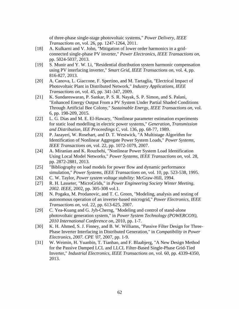
62
of three-phase single-stage photovoltaic systems," Power Delivery, IEEE
Transactions on, vol. 26, pp. 1247-1264, 2011.
[18] A. Kulkarni and V. John, "Mitigation of lower order harmonics in a grid-
connected single-phase PV inverter," Power Electronics, IEEE Transactions on,
pp. 5024-5037, 2013.
[19] S. Munir and Y. W. Li, "Residential distribution system harmonic compensation
using PV interfacing inverter," Smart Grid, IEEE Transactions on, vol. 4, pp.
816-827, 2013.
[20] A. Canova, L. Giaccone, F. Spertino, and M. Tartaglia, "Electrical Impact of
Photovoltaic Plant in Distributed Network," Industry Applications, IEEE
Transactions on, vol. 45, pp. 341-347, 2009.
[21] K. Sundareswaran, P. Sankar, P. S. R. Nayak, S. P. Simon, and S. Palani,
"Enhanced Energy Output From a PV System Under Partial Shaded Conditions
Through Artificial Bee Colony," Sustainable Energy, IEEE Transactions on, vol.
6, pp. 198-209, 2015.
[22] L. G. Dias and M. E. El-Hawary, "Nonlinear parameter estimation experiments
for static load modelling in electric power systems," Generation, Transmission
and Distribution, IEE Proceedings C, vol. 136, pp. 68-77, 1989.
[23] P. Jazayeri, W. Rosehart, and D. T. Westwick, "A Multistage Algorithm for
Identification of Nonlinear Aggregate Power System Loads," Power Systems,
IEEE Transactions on, vol. 22, pp. 1072-1079, 2007.
[24] A. Miranian and K. Rouzbehi, "Nonlinear Power System Load Identification
Using Local Model Networks," Power Systems, IEEE Transactions on, vol. 28,
pp. 2872-2881, 2013.
[25] "Bibliography on load models for power flow and dynamic performance
simulation," Power Systems, IEEE Transactions on, vol. 10, pp. 523-538, 1995.
[26] C. W. Taylor, Power system voltage stability: McGraw-Hill, 1994.
[27] R. H. Lasseter, "MicroGrids," in Power Engineering Society Winter Meeting,
2002. IEEE, 2002, pp. 305-308 vol.1.
[28] N. Pogaku, M. Prodanovic, and T. C. Green, "Modeling, analysis and testing of
autonomous operation of an inverter-based microgrid," Power Electronics, IEEE
Transactions on, vol. 22, pp. 613-625, 2007.
[29] C. Yea-Kuang and G. Jyh-Cherng, "Modeling and control of stand-alone
photovoltaic generation system," in Power System Technology (POWERCON),
2010 International Conference on, 2010, pp. 1-7.
[30] K. H. Ahmed, S. J. Finney, and B. W. Williams, "Passive Filter Design for Three-
Phase Inverter Interfacing in Distributed Generation," in Compatibility in Power
Electronics, 2007. CPE '07, 2007, pp. 1-9.
[31] W. Weimin, H. Yuanbin, T. Tianhao, and F. Blaabjerg, "A New Design Method
for the Passive Damped LCL and LLCL Filter-Based Single-Phase Grid-Tied
Inverter," Industrial Electronics, IEEE Transactions on, vol. 60, pp. 4339-4350,
2013.

63
[32] P. Acuna, L. Moran, M. Rivera, J. Dixon, and J. Rodriguez, "Improved Active Power Filter Performance for Renewable Power Generation Systems," Power Electronics, IEEE Transactions on, vol. 29, pp. 687-694, 2014.
[33] M. G. Villalva, J. R. Gazoli, and E. R. Filho, "Modeling and circuit-based simulation of photovoltaic arrays," in Power Electronics Conference, 2009. COBEP '09. Brazilian, 2009, pp. 1244-1254.
[34] H. S. Rauschenbach, "Solar cell array design handbook-The principles and technology of photovoltaic energy conversion," 1980.
[35] C. Hui, Z. Hui, J. Wentao, and W. Santong, "Research on PQ Control Strategy for PV Inverter in the Unbalanced Grid," in Power and Energy Engineering Conference (APPEEC), 2012 Asia-Pacific, 2012, pp. 1-3.
[36] P. Fang Zheng, "Application issues of active power filters," Industry Applications Magazine, IEEE, vol. 4, pp. 21-30, 1998.
[37] H. L. Jou, "Performance comparison of the three-phase active-power-filter algorithms," Generation, Transmission and Distribution, IEE Proceedings-, vol. 142, pp. 646-652, 1995.
[38] J. Si-Hun, S. SeoEun, and P. Jung-Wook, "On Improving Distortion Power Quality Index in Distributed Power Grids," Smart Grid, IEEE Transactions on, vol. 4, pp. 586-595, 2013.
[39] L. Tao and A. Domijan, "On power quality indices and real time measurement," Power Delivery, IEEE Transactions on, vol. 20, pp. 2552-2562, 2005.
[40] S. M. Halpin, "Comparison of IEEE and IEC harmonic standards," in Power Engineering Society General Meeting, 2005. IEEE, 2005, pp. 2214-2216 Vol. 3.
[41] Available: http://www.grainger.com/content/safety-electrical-power-system-
harmonics

64
APPENDICES

65
Appendix A
Crossed Frequency Admittance Matrix of Composite Load
Table A-1 DBR Matrix
(DBR: 0.67kW with 120V AC power)
0.08∠22.00° 0.15∠-145.39° 0.12∠4.36° 0.04∠-128.50° 0.07∠-96.07° 0.04∠-97.07° 0
0.06∠-137.00° 0.38∠49.34° 0.29∠-163.58° 0.17∠13.94° 0.07∠-63.94° 0.10∠99.93° 0.18∠65.00°
0.03∠76.00° 0.27∠-125.28° 0.38∠40.04° 0.32∠-168.50° 0.06∠-23.73° 0.03∠-45.48° 0.05∠145.87°
0.01∠-25.00° 0.06∠59.86° 0.24∠-132.11° 0.41∠35.77° 0.31∠177.78° 0.14∠-33.37° 0.05∠-42.37°
0.01∠-90.00° 0.08∠84.92° 0.09∠61.91° 0.25∠-139.35° 0.48∠33.26° 0.31∠174.67° 0.08∠-7.74°
0.01∠142.00° 0.06∠-85.55° 0.03∠97.14° 0.09∠56.82° 0.31∠-134.84° 0.46∠37.03° 0.29∠-178.74°
0 0.02∠-70.87° 0.05∠-76.69° 0.03∠72.41° 0.09∠73.95° 0.29∠-133.32° 0.52∠34.79°

66
Table A-2 CFL Matrix
(CFL: 15W with 120V AC power)
0.0016∠38.00° 0.0023∠-133.36° 0 0.0015∠-97.12° 0.0018∠-88.29° 0.002∠-57.10° 0.0023∠-79.83°
0.0012∠-81.00° 0.0058∠83.31° 0.0037∠-148.97° 0.0036∠63.03° 0.0045∠-113.27° 0.0034∠144.30° 0.0049∠139.50°
0.0008∠172.00° 0.0059∠--60.59° 0.0076∠78.08° 0.0079∠-123.18° 0.0076∠-22.81° 0.0019∠-50.85° 0.0039∠7.03°
0 0.0034∠107.18° 0.0145∠-31.62° 0.0207∠71.80° 0.0069∠-152.46° 0.0101∠33.42° 0.0094∠-57.11°
0 0.0011∠108.69° 0.0073∠-171.54° 0.0132∠-64.63° 0.0134∠80.29° 0.0149∠-143.40° 0.0098∠-27.19°
0.0026∠-86.56° 0.0259∠-44.56° 0.0469∠-4.72° 0.0457∠69.96° 0.0286∠-8.84° 0.0665∠80.06° 0.0423∠-52.52°
0 0.0020∠--61.40° 0.0025∠-23.92° 0.0028∠98.85° 0.0075∠-166.76° 0.0136∠--46.33° 0.0230∠80.89°

67
Table A-3 PAVC Matrix
(DBR: 0.9kW with 120V AC power)
0.0966∠ -5.00° 0.0178∠-174.81° 0.0101∠164.85° 0 0 0 0
0.0080∠156.00° 0.0771∠3.7301° 0.0137∠96.76° 0.0030∠173.73° 0 0.0012∠86.00° 0
0.0046∠7.00° 0.0118∠-6.60° 0.0839∠5.01° 0.0034∠68.28° 0.0016∠98.91° 0.0008∠-153.50° 0.0003∠-113.10°
0.0010∠-86.00° 0.0011∠-59.29° 0.0028∠-61.91° 0.0908∠5.54° 0 0 0
0 0.0010∠68.94° 0.0007∠-73.71° 0.0009∠-72.93° 0.0929∠4.3399° 0 0
0 0.0010∠32.54° 0 0 0.0286∠-8.84° 0.0940∠80.06° 0
0 0.0006∠10.60° 0 0 0 0 0.0945∠2.80°

68
Appendix B
Line Data Calculation of the Study System
Line Construction Types:
C
G
a bD
24” 24”
30”
a
b
c
G
A
30” 30”
10”
42”
Ground wire position is at 45
feet for all pole types
a
b
c
G
B
18”
36”
18”
G
c
6”
36”
c’
Same for A and
B phases

69
Table B-1 Line Data of the Study System
In the initial design all phase conductors are either 336,400 - 26/7 strands ACSR or 4/0 -
6/1 strands ACSR. See line data for each line section’s configuration and size. Neglect
line capacitance. Ground conductors are all 2/0 – 6/1 strands ACSR
Type A336 Impedance:
𝑍𝑎𝑏𝑐 = [0.4503 + 1.0721𝑖 0.1722 + 0.5045𝑖 0.1723 + 0.4265𝑖
0.1722 + 0.5045𝑖 0.4501 + 1.0728𝑖 0.1722 + 0.5045𝑖0.1723 + 0.4265𝑖 0.1722 + 0.5045𝑖 0.4503 + 1.0721𝑖
] (Ω/mi)
Line
Number From Bus To Bus
Line Length
(Miles) Phasing
Conductor
Type and Code
1 10 20 0.48 ABC A 336
2 20 30 0.4 ABC A 336
3 30 31 0.2 AB D 4/0
4 30 34 0.45 ABC B 4/0
4 30 40 0.5 ABC B 336
5 31 32 0.2 A C 4/0
6 31 33 0.2 B C 4/0
7 40 41 0.5 ABC B 4/0
8 40 50 0.6 ABC B 336
9 50 51 0.4 AB D 4/0
10 50 60 0.55 ABC B 336
11 60 61 0.4 ABC B 4/0
12 60 62 0.6 C C 4/0

70
Type B4/0 Impedance:
𝑍𝑎𝑏𝑐 = [0.5450 + 1.4311𝑖 0.1021 + 0.4886𝑖 0.1053 + 0.3924𝑖0.1021 + 0.4886𝑖 0.5497 + 1.4134𝑖 0.1082 + 0.4665𝑖0.1053 + 0.3924𝑖 0.1082 + 0.4665𝑖 0.5574 + 1.3863𝑖
] (Ω/mi)
Type B336 Impedance:
𝑍𝑎𝑏𝑐 = [0.3780 + 1.2981i 0.1021 + 0.4886i 0.1053 + 0.3924i0.1021 + 0.4886i 0.3827 + 1.2804i 0.1082 + 0.4665i0.1053 + 0.3924i 0.1082 + 0.4665i 0.3904 + 1.2533i
] (Ω/mi)
Type C4/0 Impedance:
𝑍𝑐 = [0.3333 + 0.9913𝑖] (Ω/mi)
Type D4/0 Impedance:
𝑍𝑎𝑏 = [0.5560 + 1.3908𝑖 0.1110 + 0.3378𝑖0.1110 + 0.3378𝑖 0.5560 + 1.3908𝑖
] (Ω/mi)

71
Appendix C
Simulation Models and Matlab Codes
1. Test System Simulation Model
Figure C-1: Microgrid Test System
Discrete,Ts = 1e-005 s.
powergui
v+-
v+-
v+-
v+-
v+-
A
B
C
A B C
A B C
A
B
C
A B C
A B C
A B C
A B C
29+273.15
Temperature
[K]
In1
In2
Conn1
Conn2
Conn3
Subsystem2
In1
In2
Conn1
Conn2
Conn3
Subsystem1
In1
In2
Conn1
Conn2
Conn3
Subsystem
Vabc
Ia
Ib
Ic
Nonlinear_load_model
[V62]
[V51_B]
[V51_A]
[V33]
[V32]
[I62]
[I51_B]
[I51_A]
-T-
-T-
-T-
From
i+
-
i+
-
i+
-
i+
-
i+
-
789
A
B
C
Bus10(slack_bus)
A
B
C
a
b
c
B61
A B C
a b cB60
A B C
a b cB50
A
B
C
a
b
c
B41
A B C
a b cB40
A
B
C
a
b
c
B34
A B C
a b cB30
A B C
a b cB20

72
2. Composite Nonlinear Load Simulation Model
Figure C-2: Three Phase Nonlinear Load Connection
Figure C-3: Nonlinear Load by Cross Frequency Admittance Matrix
3 Ic
2 Ib
1 Ia
In1Out1
nonlinear_load_c
In1Out1
nonlinear_load_b
In1Out1
nonlinear_load_a
s -+
Controlled Current Source2
s -+
Controlled Current Source1
s -+
Controlled Current Source
1
Vabc
DBR 0.67kW per
Load in WDBR percentage
CFL15W
Load in WCFL percentage
PAVC 0.9 kW
Load in WPAVC percentage
1
Out1
Voltage v ol_matrix
matrix_cal
In1Out1
current_waveform2
In1Out1
current_waveform1
In1Out1
current_waveform
Matrix
Multiply
Matrix
Multiply
Matrix
Multiply
1/9000.1
1/150.1
1/6700.1
10e3
Y2
Constant6
10e3
Y1
Constant3
10e3
Y
Constant1
Add
1
In1
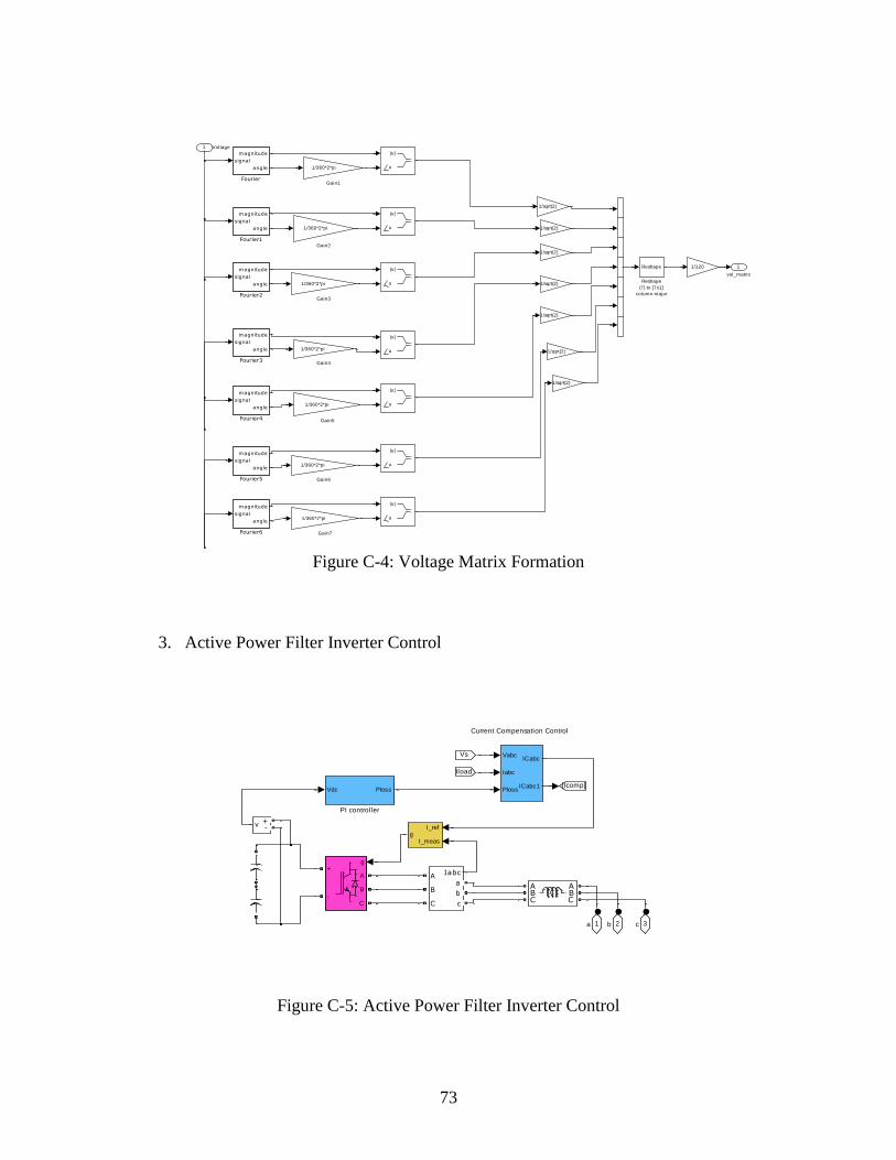
73
Figure C-4: Voltage Matrix Formation
3. Active Power Filter Inverter Control
Figure C-5: Active Power Filter Inverter Control
1
vol_matrix
Reshape
Reshape
(7) to [7x1]
column-major
|u|
u
|u|
u
|u|
u
|u|
u
|u|
u
|u|
u
|u|
u
1/sqrt(2)
1/sqrt(2)
1/360*2*pi
Gain7
1/360*2*pi
Gain6
1/360*2*pi
Gain5
1/360*2*pi
Gain4
1/360*2*pi
Gain3
1/360*2*pi
Gain2
1/120
1/sqrt(2)
1/sqrt(2)
1/sqrt(2)
1/sqrt(2)
1/sqrt(2)
1/360*2*pi
Gain1
signal
magnitude
angle
Fourier6
signal
magnitude
angle
Fourier5
signal
magnitude
angle
Fourier4
signal
magnitude
angle
Fourier3
signal
magnitude
angle
Fourier2
signal
magnitude
angle
Fourier1
signal
magnitude
angle
Fourier
1 Voltage
Current Compensation Control
3c2b1a
v+-
IabcA
B
C
a
b
c
g
A
B
C
+
-
ABC
ABC
Vabc
Iabc
Ploss
ICabc
ICabc1Vdc Ploss
PI controller
I_ref
I_measg
[Icomp]
Vs
Iload

74
4. DC Battery Droop Control Blocks
Figure C-6: Active Power Calculation
Figure C-7: Voltage Reference in dq Axis
6
ICq
5
ICd
4
VIdq
3
VIdd
2
Q
1
P
abc
sin_cos
dq0
abc_to_dq0Transformation3
abc
sin_cos
dq0
abc_to_dq0Transformation1
abc
sin_cos
dq0
abc_to_dq0Transformation
Terminator2
Terminator1
Terminator
Product3
Product2
Product1
Product
In Mean
Discrete Mean value1
In Mean
Discrete Mean value
Add1
Add
4
sin
3
Iinv
2
VId
1
Ic
f5
f
4
sin
3
w
2
VIdq*
1
VIdd*
abc
sin_cos
dq0
abc_to_dq0Transformation
sin
Trigonometric
Function4
sin
Trigonometric
Function3
sin
Trigonometric
Function2
cos
Trigonometric
Function1
sin
Trigonometric
Function
Terminator
Product2
Product1
Product
mod
Math
Function
1
s
Integrator
1e-5
Gain2
2*pi
Gain15e-6
Gain
(2/3)*pi
Constant4
(2/3)*pi
Constant3
2*pi
Constant
Add1
Add
5
E0
4
Q
3
fn
2
P
1
Pn

75
Figure C-8: PWM Signal Generation
5. System Impedance Calculation Example (from Bus 10 to Bus 30)
%%Calculate impedance from Bus 10 TO BUS 30
%%Phase ABC %%From Bus 10 To Bus 20 length 0.48mi %%A336
%% Impedance ohms per mile Zaa=0.3733+i*1.413; Zbb=0.3733+i*1.413; Zcc=0.3733+i*1.413;
Zab=0.09528+i*0.8451; Zac=0.09528+i*0.7674; Zbc=0.09528+i*0.8451;
Zww=0.8013+i*1.603; Zwa=0.09528+i*0.7857; Zwb=0.09528+i*0.7848; Zwc=0.09528+i*0.7857;
Zabc=[Zaa Zab Zac Zwa; Zab Zbb Zbc Zwb; Zac Zbc Zcc Zwc; Zwa Zwb Zwc Zww;]
%****************************** %Kron Reduction
1
PWM
5
k1
5
k
dq0
sin_cos
abc
dq0_to_abcTransformation
Scope1
Scope
Product2
Product1
Product
Signal(s) Pulses
PWM Generator
Memory1
Memory
-K-
Gain3
-K-
Gain2
PI
DiscretePI Controller1
PI
DiscretePI Controller
0
Constant10
Constant8
sin7
w
6
Ioq
5
Iod
4
VIdq
3
VIdq*
2
VIdd
1
VIdd*

76
K=Zabc(1:3,1:3); L=Zabc(1:3,4); M=Zabc(4,4); Lt=Zabc(4,1:3); Zabc_sim=K-L*inv(M)*Lt
%Length 0.48 mi Zabc_10_20=Zabc_sim*0.48;
%%From Bus 20 To 30 length 0.4mi Zabc_20_30=Zabc_sim*0.4;
Zabc_com=[Zabc_10_20 Zabc_20_30; Zabc_20_30.' Zabc_10_20+Zabc_20_30;];
%%Impedance from Bus 10 To Bus 30
Zabc10_30=Zabc_com
6. Crossed Frequency Admittance Matrix Calculation Example (PAVC)
%%%%%%%%%%%%%PAVC Matrix 0.9kW %%%%%%%%%%%%%%
%% in this case only 1st, 3rd, 5th, 7th, 9th, 11th, 13th, 15th Y2=zeros(7,7);
%%120 V rms V1=120;
I1=zeros(1,7); I1(1,1)=16.4*cos(-5/180*pi)+16.4*sin(-5/180*pi)*j; I1(1,2)=1.36*cos(156/180*pi)+1.36*sin(156/180*pi)*j; I1(1,3)=0.78*cos(7/180*pi)+0.78*sin(7/180*pi)*j; I1(1,4)=0.172*cos(-86/180*pi)+0.172*sin(-86/180*pi)*j; I1(1,5)=0.057*cos(171/180*pi)+0.057*sin(171/180*pi)*j; I1(1,6)=0.044*cos(72.8/180*pi)+0.044*sin(72.8/180*pi)*j; I1(1,7)=0.034*cos(-1/180*pi)+0.034*sin(-1/180*pi)*j;
for k=1:1:7; Y2(k,1)=I1(1,k)/sqrt(2)/V1;
end
%%120*10% V rms 60degree 3rd harmonics

77
V3=120*0.1*cos(60/180*pi)+120*0.1*sin(60/180*pi)*j;
I2=zeros(1,7); I2(1,1)=16.3*cos(-6/180*pi)+16.3*sin(-6/180*pi)*j; I2(1,2)=1.85*cos(111/180*pi)+1.85*sin(111/180*pi)*j; I2(1,3)=0.93*cos(16/180*pi)+0.93*sin(16/180*pi)*j; I2(1,4)=0.174*cos(-80/180*pi)+0.174*sin(-80/180*pi)*j; I2(1,5)=0.07*cos(162/180*pi)+0.07*sin(162/180*pi)*j; I2(1,6)=0.06*cos(78.2/180*pi)+0.06*sin(78.2/180*pi)*j; I2(1,7)=0.038*cos(12.5/180*pi)+0.038*sin(12.5/180*pi)*j;
for k=1:1:7; Y2(k,2)=(I2(1,k)/sqrt(2)-Y2(k,1)*V1)/V3;
end
%%120*5% V rms 100degree 5th harmonics
V5=120*0.05*cos(100/180*pi)+120*0.05*sin(100/180*pi)*j;
I3=zeros(1,7); I3(1,1)=16.4*cos(-5.3/180*pi)+16.4*sin(-5.3/180*pi)*j; I3(1,2)=1.45*cos(159/180*pi)+1.45*sin(159/180*pi)*j; I3(1,3)=0.98*cos(53/180*pi)+0.98*sin(53/180*pi)*j; I3(1,4)=0.16*cos(-79/180*pi)+0.16*sin(-79/180*pi)*j; I3(1,5)=0.052*cos(167/180*pi)+0.052*sin(167/180*pi)*j; I3(1,6)=0.045*cos(69/180*pi)+0.045*sin(69/180*pi)*j; I3(1,7)=0.035*cos(1/180*pi)+0.035*sin(1/180*pi)*j;
for k=1:1:7; Y2(k,3)=(I3(1,k)/sqrt(2)-Y2(k,1)*V1)/V5;
end
%%120*5% V rms 50degree 7th harmonics
V7=120*0.05*cos(50/180*pi)+120*0.05*sin(50/180*pi)*j;
I4=zeros(1,7); I4(1,1)=16.4*cos(-5/180*pi)+16.4*sin(-5/180*pi)*j; I4(1,2)=1.37*cos(157/180*pi)+1.37*sin(157/180*pi)*j; I4(1,3)=0.77*cos(9/180*pi)+0.77*sin(9/180*pi)*j; I4(1,4)=0.645*cos(46/180*pi)+0.645*sin(46/180*pi)*j; I4(1,5)=0.05*cos(173/180*pi)+0.05*sin(173/180*pi)*j; I4(1,6)=0.04*cos(69/180*pi)+0.04*sin(69/180*pi)*j; I4(1,7)=0.034*cos(-5/180*pi)+0.034*sin(-5/180*pi)*j;

78
for k=1:1:7; Y2(k,4)=(I4(1,k)/sqrt(2)-Y2(k,1)*V1)/V7;
end
%%120*5% V rms 45degree 9th harmonics
V9=120*0.05*cos(45/180*pi)+120*0.05*sin(45/180*pi)*j;
I5=zeros(1,7); I5(1,1)=16.4*cos(-5/180*pi)+16.4*sin(-5/180*pi)*j; I5(1,2)=1.36*cos(156/180*pi)+1.36*sin(156/180*pi)*j; I5(1,3)=0.77*cos(7.7/180*pi)+0.77*sin(7.7/180*pi)*j; I5(1,4)=0.165*cos(-85/180*pi)+0.165*sin(-85/180*pi)*j; I5(1,5)=0.76*cos(53/180*pi)+0.76*sin(53/180*pi)*j; I5(1,6)=0.042*cos(68/180*pi)+0.042*sin(68/180*pi)*j; I5(1,7)=0.035*cos(-4/180*pi)+0.035*sin(-4/180*pi)*j;
for k=1:1:7; Y2(k,5)=(I5(1,k)/sqrt(2)-Y2(k,1)*V1)/V9;
end
%%12*0.1 rms 70 degree 11th harmonics V11=120*0.1*cos(70/180*pi)+120*0.1*sin(70/180*pi)*j;
I6=zeros(1,7); I6(1,1)=16.4*cos(-5/180*pi)+16.4*sin(-5/180*pi)*j; I6(1,2)=1.38*cos(156/180*pi)+1.38*sin(156/180*pi)*j; I6(1,3)=0.78*cos(6/180*pi)+0.78*sin(6/180*pi)*j; I6(1,4)=0.17*cos(-88/180*pi)+0.17*sin(-88/180*pi)*j; I6(1,5)=0.063*cos(165/180*pi)+0.063*sin(165/180*pi)*j; I6(1,6)=1.64*cos(72/180*pi)+1.64*sin(72/180*pi)*j; I6(1,7)=0.038*cos(1/180*pi)+0.038*sin(1/180*pi)*j;
for k=1:1:7; Y2(k,6)=(I6(1,k)/sqrt(2)-Y2(k,1)*V1)/V11;
end
%%120*0.05 rms 30 degree 13th harmonics V13=120*0.05*cos(30/180*pi)+120*0.05*sin(30/180*pi)*j;
I7=zeros(1,7);
I7(1,1)=16.4*cos(-5/180*pi)+16.4*sin(-5/180*pi)*j; I7(1,2)=1.36*cos(156/180*pi)+1.36*sin(156/180*pi)*j; I7(1,3)=0.78*cos(6.8/180*pi)+0.78*sin(6.8/180*pi)*j; I7(1,4)=0.172*cos(-86/180*pi)+0.172*sin(-86/180*pi)*j; I7(1,5)=0.06*cos(170/180*pi)+0.06*sin(170/180*pi)*j;

79
I7(1,6)=0.045*cos(73/180*pi)+0.045*sin(73/180*pi)*j; I7(1,7)=0.83*cos(31.5/180*pi)+0.83*sin(31.5/180*pi)*j;
for k=1:1:7; Y2(k,7)=(I7(1,k)/sqrt(2)-Y2(k,1)*V1)/V13;
end
Y2
for x=1:1:7 for y=1:1:7
fprintf('%4.4f %4.4f\n',abs(Y2(x,y)),angle(Y2(x,y))/pi*180);
end end