integrating microgrid power for net-zero energy …
TRANSCRIPT
INTEGRATING MICROGRID POWER FOR NET-ZERO
ENERGY SUPPLY CHAIN OPERATIONS:
A BIG DATA ANALYTICS
APPROACH
by
An Pham, B.S.
A thesis submitted to the Graduate Council
of Texas State University in partial fulfillment
of the requirements for the degree of
Master of Science with a Major in
Industrial Engineering
August 2018
Committee Members:
Tongdan Jin, Chair
Clara Novoa
Cecilia Temponi
COPYRIGHT
by
An Pham
2018

FAIR USE AND AUTHOR’S PERMISSION STATEMENT
Fair Use
This work is protected by the Copyright Laws of the United States (Public Law 94-553,
section 107). Consistent with fair use as defined in the Copyright Laws, brief quotations
from this material are allowed with proper acknowledgment. Use of this material for
financial gain without the author’s express written permission is not allowed.
Duplication Permission
As the copyright holder of this work I, An Pham, authorize duplication of this work, in
whole or in part, for educational or scholarly purposes only.

iv
ACKNOWLEDGEMENTS
I would like to thank my thesis advisor, Dr. Tongdan Jin in the Ingram School of
Engineering at Texas State University for all his endless support in guiding me in my
research and giving me valuable life advice. He has always been there to support and give
helpful guidance whenever I needed his help.
I would also like to thank Dr. Clara Novoa in the Ingram School of Engineering at
Texas State University who is always there to provide insightful help and support. I would
like to extend my gratitude to her for advising me in enhancing my research capabilities.
I would also like to thank Dr. Cecilia Temponi in the McCoy School of Business
at Texas State University who is always there to guide the research from a business
perspective. I would like to extend my gratitude to her for encouraging me to pursue a
Ph.D.
I would like to thank Dr. Zong in the Computer Science Department at Texas State
University for providing research fund support and technical assistance to my research.
I would also like to thank all the professors and staff of the Ingram School of
Engineering at Texas State University in extending their guidance throughout my school
years. Last but not least, I would express my appreciation to the US Department of
Agriculture for funding my thesis project under the B-GREEN Grant (#2011-38422-
30803), and to the National Science Foundation for partly supporting me with under the
NSF Grant (# 1522318).

v
TABLE OF CONTENTS
Page
ACKNOWLEDGEMENTS ............................................................................................... iv
LIST OF TABLES ............................................................................................................ vii
LIST OF FIGURES ........................................................................................................... ix
CHAPTER
I. LITERATURE REVIEW .................................................................................... 1
1.1 Energy Efficiency ................................................................................... 3
1.2 Carbon Tax, Cap and Trade .................................................................... 5
1.3 Power Purchase Agreement .................................................................... 8
1.4 Onsite renewable energy generation ..................................................... 12
1.5 Microgrid Systems ................................................................................ 14
1.6 Research Objectives .............................................................................. 15
II. INDUSTRY PRACTICE OF RENEWABLE INTEGRATION ..................... 19
2.1 Manufacturing Industries ...................................................................... 19
2.2 Service Industry .................................................................................... 24
III. WIND TURBINE AND PV CAPACITOR MODEL AND ELECTRIC
VEHICLE ENERGY INTENSITY ...................................................................... 42
3.1. Wind Turbine Capacitor Factor ........................................................... 42
3.2. Solar PV Capacitor Factor (in Northern Hemisphere) ......................... 44
3.3 Electric Vehicle Energy Intensity Rate ................................................. 47
vi
IV. NET ZERO CARBON MANUFACTURING FOR SINGLE
FACILITY PLUS WAREHOUSE AND E-TRANSPOR
DETERMINISTIC DEMAND ................................................................... 49
4.1 Systems and Model Settings ................................................................. 49
4.2 Optimization Algorithm ........................................................................ 50
4.3. Climate Data ........................................................................................ 56
4.4. Numerical Experiment ......................................................................... 69
4.5 Conclusion ............................................................................................ 75
V. INTEGRATING MICROGRID POWER FOR NET-ZERO ENERGY
PRODUCTION-LOGISTICS WITH DEMAND UNCERTAINTY.................... 77
5.1 Model Setting ........................................................................................ 77
5.2 A Stochastic Optimization Model ......................................................... 79
5.3 Heuristic Approach to Solve Stochastic Optimization Model .............. 82
5.4 Numerical Experiment for Single Factory – Single Warehouse
Model .......................................................................................................... 84
5.5 Multi-Factory Production and Logistics Systems ................................. 90
VI. NET ZERO CARBON SUPPLY CHAIN NETWORK UNDER
DETERMINISTIC AND STOCHASTIC DEMAND .......................................... 96
6.1 Supply Chain with Microgrid Power and Deterministic Demand ........ 96
6.2 Supply Chain System with Microgrid Power and Stochastic
Demand ............................................................................................................... 121
VII. CONCLUSIONS AND FUTURE WORK.................................................. 133
APPENDIX SECTION ................................................................................................... 135
REFERENCES ............................................................................................................... 144
vii
LIST OF TABLES
Table Page
3.1. Hellmann Exponent ................................................................................................... 44
3.2. Key Parameters in Solar PV Power Generation ........................................................ 45
4.1. The Notation for the Problem .................................................................................... 54
4.2. Average Wind Speed and Weather Conditions of Six Cities .................................... 65
4.3. Wind Speed of Week 1 in Wellington (unit: m/s) ..................................................... 66
4.4. Daily Weather Condition from 2006 to 2016 in Wellington ..................................... 67
4.5. The Probabilities of Weather States for Week 1 in Wellington ................................ 68
4.6. Weather Coefficients under Different States ............................................................. 68
4.7. Production, Inventory, Backorders, Logistics and Energy Data................................ 70
4.8. Machine and Labor Resources in the Factory ........................................................... 71
4.9. Cost and Operation Parameters of WT and PV systems ........................................... 72
4.10. Factory and Warehouse locations ............................................................................ 74
4.11. Optimal Solutions of Onsite Generation Capacity .................................................. 74
5.1. Model Parameters and Decision Variables ................................................................ 78
5.2. Cost and Operation Parameters of WT and PV systems ........................................... 85
5.3. Machine and Labor Resources in the Factory ........................................................... 86
5.4. Cost and Operation Parameters of WT and PV systems ........................................... 87
5.5. Results of Three Different Production-Logistics Systems ........................................ 89
5.6. Average weather condition of 4 cities ....................................................................... 90
5.7. Production demand for two factories ......................................................................... 92
5.8. Comparisons under Different PV Cost and Carbon Credits ...................................... 94
5.9. Levelized Cost of Renewable Energy ........................................................................ 95
6.1. Average Wind Speed and Weather Conditions of Ten Cities ................................. 103
6.2. Production, Inventory, Backorder, Shipping, and Energy Data .............................. 105
6.3. Product demand for 52-week planning .................................................................... 106
6.4. Cost and Operation Parameters of WT and PV systems ......................................... 107
6.5. Labor and Machine Resources in the Factory ......................................................... 108
6.6. Results of Production-Logistics Systems -Two Scenarios ...................................... 111
6.7. Results of Production-Logistics System without Carbon Credits ........................... 112
6.8. Product Demand for 52 Weeks ................................................................................ 115
6.9. Labor and Machine Resource Available .................................................................. 116
6.10. Comparison under Different PV cost and Carbon Credits .................................... 120
6.11. Production Demand ............................................................................................... 123
6.12. Results of Production-Logistics Systems of Two Cases ....................................... 127
viii
6.13. Capacity Output of Two Cases without Carbon Credits ....................................... 128
6.14. Mean and Standard Deviation of Demand for Product A and Product B .............. 129
6.15. Optimization of Onsite Generation Capacity......................................................... 132

ix
LIST OF FIGURES
Figure Page
2.1. SKY on-site renewable energy .................................................................................. 38
3.1. Weibull Wind Speed Distributions ............................................................................ 43
4.1. A single facility and warehouse setting with onsite generation................................. 49
4.2. Wellington Weather Condition in 2016 ..................................................................... 57
4.3. Wellington Average Wind Speed at the Height of 80 Meters ................................... 57
4.4. Weather conditions of Christchurch in the 2016 ....................................................... 58
4.5. Weather conditions of Aswan in 2016 ....................................................................... 59
4.6. Average Wind Speed of Aswan at the 80-meter height in 2016 ............................... 59
4.7. Weather conditions of Luxor in 2016 ........................................................................ 60
4.8. Average Wind Speed of Luxor at the 80-meter height in 2016 ................................. 61
4.9. Weather Condition of Yuma in 2016 ......................................................................... 62
4.10. Average Wind Speed of Yuma at the 80-meter height in 2016 ............................... 62
4.11. Weather Condition of San Francisco in 2016 .......................................................... 63
4.12. Average Wind Speed of San Francisco at the 80-meter height in 2016 .................. 64
4.13. Weekly Wind Turbine Capacity Factor of Eight Cities ........................................... 67
4.14. The Weekly Solar PV Capacity Factor of Eight Cities ........................................... 69
4.15. Production Demand of Product A and Product B .................................................... 70
4.16. Production, Inventory, and Backorder of Product A ............................................... 73
4.17. Production, Inventory, and Backorder of Product B ............................................... 74
5.1. Multi-Factory and One Distribution Center with Microgrid Generation .................. 77
5.2. Process Chart to Solve the Model (Pham et al. 2017) ............................................... 84
5.3. Decision on Product A for Model P2-1 ..................................................................... 88
5. 4. Decision on Product B for Model P2-1 .................................................................... 88
5.5. The Weekly Solar PV Capacity Factor of Eight Cities ............................................. 91
5.6. Results of Product A .................................................................................................. 93
5.7. Results of Product A .................................................................................................. 93
6.1. Supply Chain with Microgrid Generation ................................................................. 97
6.2. Weekly Wind Turbine Capacity Factor of Ten Cities ............................................. 104
6.3. Weekly Solar PV Capacity Factor of Ten Cities ..................................................... 104
6.4. Decision Variables Output of Product A ................................................................. 109
6.5. Decision Variables Output of Product B ................................................................. 109
6.6. Scenario I Supply Chain layout ............................................................................... 110
6.7. Scenario II layout ..................................................................................................... 110
x
6.8. Supply Chain Layout with Distance for Travel ....................................................... 114
6.9. Production Quantity of Product A ........................................................................... 117
6.10. Inventory-Backorder Level of Product A .............................................................. 118
6.11. Production Quantity of Product B ......................................................................... 118
6.12. Inventory- Backorder Level of Product B ............................................................. 119
6.13. Production Output of Product A for Case I ........................................................... 123
6.14. Production Output of Product B for Case I............................................................ 124
6.15. Production Output of Product A for Case I ........................................................... 124
6.16. Production Output of Product B for Case II .......................................................... 125
6.17. Case 1 Supply Chain Network ............................................................................... 126
6.18. Case 2 Supply Chain Network ............................................................................... 126
6.19. Supply Chain Layout with Distance Travel ........................................................... 129
6.20. Production Output for Product A ........................................................................... 130
6.21. Production Output for Product B ........................................................................... 130
6.22. Inventory-Backorder level for Product B .............................................................. 131

1
I. LITERATURE REVIEW
Since the industrial revolution, there is a rise in temperature and sea level, as well
as worsening heat waves and extreme weather conditions including hurricanes and
tornadoes. Seasons like spring arrive earlier and ice sheets are melting while the oceans
are acidifying. “In January, weather researchers confirmed that 2015 was the hottest year
worldwide since record keeping began in the 19th century, eclipsing 2014, which
previously held the record. The vast majority of scientists say human activities are to
blame,” (Smith, 2016). According to the book Renewable Energy and Climate Change
(2009), in 2003 Europe experienced the most extreme heat wave which killed 70,000
people and caused 13 billion euros losses. In 2005, hurricane Katrina devastated the US
gulf coast laying waste to the city of New Orleans consequently killing 1322 people and
causing $125 billion dollars in damage. Four weeks after Katrina, Hurricane Rita caused
$14.7 billion dollars in damage and the evacuation of three million people. Currently, “in
Bangladesh, rising sea levels have forced millions to leave coastal villages along the Bay
of Bengal. In Mali, an impoverished African country, drought is making the local
farming increasingly difficult. And in the northwestern U.S., the Pacific Ocean is
encroaching upon lands the Quinault Indian Nation has lived on for thousands of years”
(Smith, 2016). Earth’s temperature has remained steady for the course of western
civilization much as a human’s body temperature remains steady through the course of
life. However, since the 19th century Earth’s average temperature rose 1.4oF. Albeit it is
a small change, it can be viewed in the same way one views a 1.4OF fever in a small
child; this rise in Earth’s temperature is a concern for human society. The difference
between now and the last ice age, when North America was covered in a half mile thick

2
ice sheet, was only 9OF. However, where the warming between then and now took
thousands of years the warming of 1.4OF took only 100 years. In fact, “the projected rate
of temperature change for this century is greater than that of any extended global
warming period over the past 65 million years. The Intergovernmental Panel on Climate
Change stated that continuing on a path of rapid increase in atmospheric CO2 could cause
another 4 to 8OF warming before the year 2100” (McKibben, 2012).
Key climate processes involve long lags, and important greenhouses gases remain
in the atmosphere for many years after they are emitted (Richard, 2016). Among all the
heat trapping gases in the atmosphere, carbon dioxide (CO2) is the most significant
contributor to the climate change. CO2 is mainly produced from human activities and
remains the longest in the atmosphere. It takes about a decade for methane (CH4)
emissions to leave the atmosphere (it converts into CO2) and about a century for nitrous
oxide (N2O) (EPA, 2016). In the case of CO2, much of today’s emissions will be gone in
a century, but about 20 percent will still exist in the atmosphere approximately for 800
years from now (Forster, 2007). In 2013, CO2 accounted for about 82% of all U.S.
greenhouse gas emissions from human activities (EPA, 2016). The most popular
activities of humankind that emit CO2 are using fossil fuel for energy and transportation
usage. Emission from burning fossil fuels are the primary cause of rapid and accelerating
growth in CO2. The combustion of fossil fuels to generate electricity is the largest single
source of CO2 emissions in the nation, accounting for about 37% of total U.S. CO2
emissions were 31% of total U.S. greenhouse gas emissions in 2013 (EPA, 2016). The
combustion of fossil fuels such as gasoline and diesel for transporting people and goods
is the second largest source of CO2 emissions, accounting for about 31% of total U.S.

3
“Based on well-established evidence, about 97% of climate scientists conclude that
humans are changing the climate” (EPA, 2016).
The International Energy Agency projects that by 2030, about 42% electricity will
need to be supplied by renewables, increasing to 57% in 2050, to stay within a 2-degree
Celsius average global warming threshold (RE100, 2016). There is a necessity for
renewable energy to be increased by 200% between now and 2030. In December 2015 a
conference was held in Paris where political leaders as well as business executives could
make critical decisions to keep world average temperature rise between a 1.5 to 2 OC.
According to the IPCC a limit of 1,000 giga-tons of CO2 cannot be emitted by human
being in order to stay within this limit, however at the current rate of emission limit will
be reached by the year 2040 (Greenpeace, 2015).
1.1 Energy Efficiency
Due to the growing energy issue which developed between 1970 and 1980 and
even after the 1986 counter oil shocks, energy efficiency has grown to become a big
attraction for sustainable economic growth. This is noticed within the context of climate
change and global warming. These two controversial subjects have given energy
efficiency a new outlook. With top issues like the increase in the price of crude oil
during the 2000s as well as the 1993 energy crisis, energy efficiency has been placed on
the top list of priorities for many countries in political agendas.
With this urgency to reduce CO2 emissions and the carbon budget running low, it
is reasonable for public policy to be enacted in order to curtail the current rate of carbon
emissions. Many governments are aware of the numerous benefits that are brought by
increasing energy efficiency for their country. This include environmental benefits such

4
as reductions in greenhouse gases as well as pollution that contaminates air, water, and
soil. Aside from this are the reduction in investments for infrastructure, improved
consumer welfare, as well as lowering of fossil fuel dependency, and increased
competitiveness.
Makidou et al. (2015) studies the energy efficiency in EU using data from 2000 to
2010. In this paper, two methodologies that were used to analyze the data include data
envelopment analysis (DEU) and multicriteria evaluation model. The results show more
improvement need to be addressed to increase the energy efficiency in EU. It suggests the
policy makers to “consider a much wider range of impacts of energy efficiency programs,
instead of focusing solely on an input-output energy economic production framework.
According to National Energy Independence Strategy, energy efficiency will
increase yearly by 1.5 percent up to 2020. It predicts that the total power consumption
during the period of 2014 to 2020 will increase up to 1.5 percent where 1.3 percent is
from natural sources. About 37 percent of total energy use in the world came from
industrial sector which use more energy than any other sector. Abdelaziz et al. (2010)
provide a review of energy saving methods in industrial fields. The review paper is
divided into three categories which include energy saving by management, by
technologies, and by policies. The use of energy saving technologies is found to be cost
effective using the equipment in the facilities to reduce the total consumptions. Together
with the public policies, the efficiency and energy saving strategies are proved to be
economically viable in most cases.
The USA consumes 25% of the world’s energy. Nevertheless, the most significant
growth of energy consumption is currently taking place in China, which has been

5
growing at 5.5% per year (International energy outlook 2009). An evaluation of the
effectiveness of China’s energy saving and emission reduction policies (ESER) in 15
energy intensive industries is conducted by Yang and Yang (2016). The data
envelopment analysis (DEA) is used to analyze the energy productivity of the selected
industries in the 10th and 11th Five-Year Plan (FYPs). The study shows that four out of
fifteen industries have significantly improved energy productivity, and the whole nation
has reduced 20 percent of energy intensity during the 11th FYPs.
Mouzon et al. (2014) developed a multi-objective optimization model which aims
to minimize the total energy consumption with the shortest completion time. The authors
consider the non-bottleneck machines to consume the large amount of energy and
develop the methodology to reduce the total energy consumption by optimizing the
production schedule. The proposed dispatching rules show to have a potential to
effectively reduce energy consumption.
Li et al. (2015) study the energy efficiency of biofuel feedstock and its related
processing improvement. The authors optimize the energy consumption of the feedstock
processing with production constraints based on the improving scenario. They consider
two different dryer structures of particle separation after grinding stage. Different
scenarios are demonstrated by applying the proposed method which includes: material
flow with no particle separation, material flow with adoption of particle separation, and
applied proposed scheduling model.
1.2 Carbon Tax, Cap and Trade
Currently there exist two main branches of policy that have been implemented
globally for the reduction of greenhouse gases, these are the carbon tax system, and the

6
carbon cap and trade system. A carbon tax is simply an excise tax imposed on carbon
emitted per ton of CO2. It can be implemented in upstream of the production as well as
downstream of the energy consumption chain. However, it is considered a tax in its
name and purpose. Hence it carries a negative connotation among policy makers in the
United States. Where a large majority of them try to amend for a more tax neutral policy
such as the cap and trade system. Under this system, Green House Gas emitters receive
allowances which they are allowed to emit. It becomes their choice to improve their
facilities to greener methods of emissions, generate less emissions, do nothing, or
purchase allowances from the emissions market. “Because emissions trading uses
markets to determine how to deal with the problem of pollution, cap and trade is often
touted as an example of effective free market environmentalism” (Tracey et al., 2010).
This produces an advantageous flexibility that is expanded upon by the U.S. policy
makers. However, cap and trade has a few underlying problems that undermine its
efficacy. At the top of the list is its complexity in terms of policy and in its ability to
actually curtail climate change and the greenhouse effect. In the U.S., the only type of
emissions market that existed was the Sulfur Dioxide market used to prevent acid rain but
it eventually collapsed in 2008. In the European Union, there is a system of cap and trade
that is being implemented, but is not considered a success due to its overwhelming
complexity.
According to the report in (Sewalk, 2013), for the foreseeable future in the United
States there exists a time span by which a cap and trade system will take to be actually
implemented as well as for a full emission regulation market to be developed. This time
span may be longer than preferable for the greenhouse gas emissions allowance will

7
allow for. With regards to a federally imposed carbon tax, there exists also precarious
problems that may undermine its effectiveness. States may choose to impose their own
CO2 tax or Renewable Portfolio Standards regardless of the existence of national climate
policy or federal CO2 tax. With a national emissions tax, there will be overlapping at
state level. However, “the maximum feasible reduction in national emissions… is higher
for a state-level Renewable Portfolio Standard compared to a state level CO2 tax,”
(Accordino and Rajagopal, 2015).
Hammami et al. (2014) introduce a mathematical model to control carbon
emission in a multi-echelon production inventory framework. The main decision is to
minimize the total system cost considering the carbon tax and carbon cap with the
constraints of lead time. The study demonstrates the “effect of individual emissions caps
on each facility with comparison to a global cap on the entire supply chain.”
Krass et al. (2013) develop different models to study the influence of environment
tax on reducing environmental pollution process. They consider to maximize the firm’s
profit with technology choices of greener technology and regular production technology.
Both technologies affect the production costs, the amount of pollutant generated, and
product selling price by considering that the consumers may not want to pay for
additional green product cost. They also study the scenario where the regulators work
with the firm to agree on the level of taxes, fixed costs, subsidies, and consumer rebates
to maximize the benefit of the social welfare,
Marti et al. (2015) introduce the mathematical approach of supply chain network
design that focuses on carbon footprint and operation trade-offs as well as on the impacts
of carbon policies and their cost effectiveness. The paper shows that the design and

8
signature of the products can heavily influence the network design, the cost, the carbon
emission control, and carbon abatement. In conclusion, the market carbon footprint cap
(MCFC) is more applicable because it has an important impact on the supply chain
network design. Furthermore, the total cost of the cap policy is lower than the tax policy.
1.3 Power Purchase Agreement
Numerous companies have committed to achieve 100% renewable energy through
Power Purchase Agreement (PPA) in combination with other methods to reduce carbon
and greenhouse gas emissions. A power purchase agreement is a solar power contract
where a developer goes on site and designs, finances, and permits the installation of a
solar energy system on the client’s site. The client is committed to a 10 to 25-year
contract which upon fulfillment he/she can expand, cancel , or purchase the system from
the developer. During the life of the contract, the developer not the client is responsible
for maintenance and upkeep of the system. According to Edge (Edge, 2015), Power
Purchase Agreements have no/low up-front cost, ability for the tax-exempt entity to enjoy
lower electricity price thanks to savings passed on from federal tax incentives,
predictable cost of electricity over 15-25 years, no need to deal with complex system
design and permits, and lastly no operating and maintenance responsibilities. There exist
some potential constraints that are inherent to Power Purchase Agreements due to
municipal laws such as debt limitations, restrictions on contracting power, budgeting
issues, public purpose and credit lending issues, public utility rules, and authority to
interests and buying electricity. The solar powered system installed by the Independent
Power Producer (or contractor) should contain a spinning reserve capable of having a
spare generation capacity in the event of power imbalance such as in the case of power

9
loss. The loading scheme on the reserve system should be arranged in such a way that
the backup should cover a preset fraction of the largest infeed on the system. “If a system
event occurs and insufficient generation reserve is available to cover the required power
demand, then load shedding will occur” (Proctor and Flynn, 2000). Therefore, in order to
have a risk-averse Power Purchase Agreement, the IPP should have a system capable of
providing partial backup to the system in contingency.
Many companies have chosen to go with Power Purchase Agreements to achieve
their goal of being supplied by 100% renewable energy to their facilities. Recently in
order to achieve the 100% renewable energy target, “Walmart went into contract to buy
58% of the estimated output from Pattern Energy Group’s new Logan’s Gap Wind farm
in Texas under a 10-year Power Purchase Agreement” (Lozanova, 2015).Walmart, the
world giant retailer, is considered the world leader in renewable energy. From 2005 to
present, the company has more than 300 renewable projects which are under
development or in operation. Its target is to procure 7,000 GWh of renewable energy per
year by 2020. In 2005, the company successfully reduced Green House Gases (GHGs) by
20% from all of its stores, distribution centers and clubs which resulted in about 3 million
metric tons of GHGs. In the Approach to Renewable Energy, Walmart reported that even
though its “square footage increased by 45% and sales grew 51%, emission grew only
about 12%” (Walmart, 2015). At present, the company has 26% of its power coming
from renewable energy sources. By purchasing Power Purchase Agreements (PPAs),
Walmart is taking a significant step in achieving its long-term goal of getting 7 billion
kilowatt-hours of renewable energy by 2020.

10
Microsoft is one of the major tech companies that “took a big step toward
transforming the energy supply chain with its biggest power purchase agreement to date
with the Pilot Hill Wind project near Chicago, Illinois, a 175-megawatt wind farm”
(Verge, 2014). Microsoft will purchase approximately 675 GWh of renewable energy
from Pilot Hill Wind which is equivalent to powering 70,000 homes. The company has
also signed two PPAs for wind generation projects with Keechi Wind Projects in Texas
which is generating up to 110 MW yearly. Microsoft made a commitment to achieving
carbon neutral in 2025. As of today, “roughly 44 percent of the electricity used by our
datacenter comes from these sources. Our goal is to pass the 50 percent milestone by the
end of 2018, top 60 percent early in the next decade, and then to keep improving from
there,” wrote Brad SmithPresident and Chief Legal Officer of Microsoft (Smith, 2016).
Davidson et al. (2015) evaluate the overall impact on the cost of systems for
customers under third party ownership. Analysis is done on contract data from 2010-
2012 consisting of 1113 contracts in that timeframe. Implication is made regarding the
timing of payment and the structure of the contract such as the higher average cost of
power purchase contracts over leases. Second it is seen that the cost of pre-paid contracts
is less than no money down contracts. Lastly power purchase agreements and leases both
cost more if they include escalator clauses within them.
Jenkins and Lim (1999) propose to look at different scenarios with various
perspectives regarding a power purchase agreement. They take an overall look at PPA
effects on the country’s economy. Central to the evaluation are sensitivity and risk
analysis which identify the most critical values that allow the model to show a probability
distribution of values rather than single predicted value. The paper then identifies those

11
who are to gain and lose from the contract. Should it be undertaken using a distributive or
stakeholder analysis allowing the partners to test the contract under various
circumstances for sustainability? This is to show the benefits of a financial or economic
stakeholder, and the analysis can be made from both PPA and Build-Operate-Transfer
(BOT) agreements.
Ferrey (2004) describes the development of small power producer initiative
among five Asian countries. These countries include Thailand, Indonesia, India, Sri
Lanka, and Vietnam. A common feature of all these nations is that they are in need of
increase in long term power generation. Most of these countries have been approached
by private developers in the deployment of small power production projects. Cost
concepts are applied in various ways for each nation. For example the payment in
Vietnam will be done based on “needed” demand regardless of whether that demand is
actually used or not.
Zeng and Yang et al. (2015) investigate the development of prices of green
energy. The article describes the detriment that a non-market guided price has done to
the development of the green energy market in several provinces of China. The paper
goes on to describe the importance of Direct Power Purchase for Large Users (DPLU) on
the reform of the electricity market. It shows that DPLU will be a critical factor that
allows the users to decide the price of electricity with the chosen generators so as to
improving the market.
In their paper, Binkley and Harsh et al. (2013) describe the different types of
electricity purchase agreements involved with anaerobic digesters on dairy farms. They
show that even possessing larger electricity production capacity, net metering’s Net

12
present value was only 6% more than the buy-all sell-all agreement on average. Also, the
limitations implicated from net metering constrain the generator size which is a
detriment, especially when larger herd size is involved. Repealing size limitations with
net metering purchase agreements will allow for high net present value.
1.4 Onsite renewable energy generation
Onsite generation, also known as distribute generation, produces electricity
through the installation of distributed energy resources (DER) locally. Typical DER units
include wind turbine, solar PV, and geothermal systems that are placed close to end
consumers. Due to its long-term contact and public policy restriction to large energy
users, large companies are working on developing onsite renewable energy generation to
supply its own power. This is an increasingly popular way of reducing GHG that is used
by many industry facilities, commercial/government building, distribution warehouses as
well as educational institutions through on-site renewable energy. Minimizing fossil fuel
emissions like carbon dioxide can be achieved with onsite wind and solar generation
which can supply partial power to a facility while reducing CO2. Aside generating public
publicity for the sites entity, it also allows for the facility to become energy independent
while reducing costs and becoming a visible demonstration of civic commitment to
environmental commitment. Another benefit is net metering which can provide positive
dividends for the facility and become a variable source of income for the entity.
IKEA, the retailer of home furnishing products, has made its pledge to power its
stores entirely by renewable energy by 2020. The company has installed solar systems on
90 percent of its stores, over 700,000 solar panels, in the U.S. locations. By 2015, the
company has spent $1.9 billion to invest in renewable energy by owning and operating its
13
own solar system. The company also operates a total of 279 wind turbines located in
Canada, Ireland, and the US.
Telsa Motors, the electric car company, targets to operate a Gigafactory in Storey
County, Nevada entirely by 100% onsite renewable energy. The renewable energy used
for the plant will be solar panels, wind farm, and geothermal electricity plant. The factory
manufacture batteries for 500,000 vehicles per year. The company plans to lower the sell
price for its car battery pack to $3000 due to the reduction of operating cost driving by
the self-supply green energy (Armstrong, 2015).
Much research has been done focusing on optimizing the onsite renewable energy
system. Roy et al. (2009) proposed a design space for different reliability levels using
chance constrained programming. The system is modeled using a probabilistic
mathematical approach which takes into consideration a wind turbine and transmission
system as well as an electrical generator. With this method, it was possible to account for
uncertainty in resource availability.
Shafer et al. (2009) discuss different types of renewable energy projects that can
benefit manufacturing companies such as net metering, selling intermittent surplus
generation, and behind-the-meter-project (i.e. onsite wind generation) in the cement
industry. It is recommended that the energy-intensive industry considers balancing the
onsite natural wind resources and avoids getting in the wind business by signing a long
term PPA for 25 years. Considering that the power demand of a cement facility is in a
range between 100 to 300MW, the paper concludes that onsite wind generation projects
benefits the heavy manufacture by creating a long-term investment in reducing the risk of
price changing for 35% of electricity needed.
14
Shigenobu et al. (2016) proposes a method of protecting a distribution system and
attaining reduction in distribution loss using cooperative controlled PVs, battery energy
storage system (BESS) and EVs. An optimization problem is formulated and solved
using Particle Swarm Optimization where the objective function is to minimize the
distribution loss and to guarantee the power quality.
Rogelj et al. (2015) makes a discussion in clarifying concepts like carbon
neutrality, climate neutrality, full decarbonization, and net zero carbon or net zero
greenhouse gas emissions (GHG). They express the confidence that with current global
pledge, there is a 66% chance to stay below the target of 2OC and achievement of net
negative CO2 emissions after 2070.
Pechmann et al. (2015) consider the financial benefit of self-supply renewable
energy grid using a case study approach. The study shows that partially self-supply
renewable energy is very promising and attractive alternative in financial terms,
especially for onsite photovoltaic system. Furthermore, the optimization in dimension of
virtual power plan can achieve further cost benefits.
1.5 Microgrid Systems
Unlike onsite or multi-node distributed generation (DG), a microgrid system
technically is an independent and self-sufficient power system which may or may not be
connected to the utility grid. For grid-interconnected microgrid, the user can choose to
operate the system in islanding mode if the supply of the main grid is interrupted or in a
failure state. In this case, new considerations must be taken for reliability design as the
islanding model essentially benefits the reliable power supply of local consumers,
especially in a contingent event. In addition, a microgrid system is considered as a viable

15
energy solution in remote areas where long distance transmission or distribution lines are
too costly to be constructed. Architecturally, both onsite generation and microgrid
systems adopt one or multiple distributed energy resource (DER) units to supply the
electricity to meet the local needs. The main difference is that the microgrid is capable of
maintaining independent and sustainable supply while onsite generation usually co-
supplies the power along with the main grid. Last, but not the least, microgrid systems
possess the unique capability of ensuring power resilience by forming an islanding model
against extreme events, including hurricane, tornados, earthquake and man-made attacks.
1.6 Research Objectives
Though carbon tax, cap and trade have their benefits in curtailing GHG, their
inherent drawbacks include the penalty mechanism and market complexity. Namely they
would permit for the day to day business of carbon emissions to continue by simply
letting companies pay their way. Although the idea of a carbon tax is to spur the
curtailing of carbon emissions, companies whose profits are large enough could
inherently continue to emit GHG as usual. While smaller companies with less profit
margin would attempt at avoiding the tax and going green by lowering their carbon
emissions, the larger companies would pursue to just pay the tax and continue polluting.
Similarly, while cap and trade poses a large obstacle for polluting firms, it would still
leave a way for companies to continue their production processes as they were before by
the acquisition of permits on the market. Although the incentive is there to cut back on
emissions by generating innovation in their market and making gains through these
breakthroughs as well as by selling and making profit from the trading of permits, the
simple logic of the cap and trade system is inherent on companies making purchase to

16
continue their production without changing their processes. Lohman (2006) argues that
carbon trading “encourages the industries most addicted to coal, oil, and gas to carry on
much as before”. Since the company can purchase cheap carbon credits, they will
continue using fossil fuel rather than renewable energy. Leonard (2009) believes that
carbon offsets reassure the companies to do unfair practices and allow firms to continue
pollution as normal practices which essentially detract from the bigger picture of global
climate change impacts.
Power purchase agreements (PPA) offer monetary as well as operational benefits,
and there are various aspects that might be looked at as negative parts of a PPA. Among
is the lack of ownership that goes with entering into a PPA. This apparent benefit with
regards to maintenance cost could leave the consumer vulnerable to drastic prices
changes in the future especially if the price costs are lower. Also, from the lack of
control in the setup of the equipment lies the project completion risk which can leave the
consumer at setback regarding projects and schedules. Furthermore, entering into PPA
will mean the loss of financial incentive programs such as grants, rebates, and carbon tax
credits.
Despite the apparent disadvantages of PPA, Carbon tax, and cap and trade, the
development of on-site renewable energy generation is very promising. Among the top
benefits that on-site generation has is although it has a higher initial investment it leaves
the consumer safe from varying price costs as well as allowing them to have ownership
and control of the electricity generation technology. Furthermore, beyond the breakeven
point the company’s utility cost, if optimized, will be at a minimum if not zero. Adding

17
to this the company through net metering can be able to turn a profit by selling excess
energy back to the grid as well as alleviate peak energy demand costs.
This thesis proposes a mathematical method to approach net zero carbon emission
in supply chain. To achieve net-zero carbon emission performance, a production-
distribution system is designed requiring the total energy consumed by transportation
network as well as the production network. This includes consumption from renewable
energy sources such as wind turbines, photovoltaic sources, and among others hydro
generators. Due to the output of hydro systems, PV, and WT being intermittent, at
sometimes power generation will be less than the demand of the production-distribution
system. In those cases, the energy gap is fulfilled using energy from fossil fuel power
plants. In order to attain net zero-carbon criteria this “borrowed” conventional energy
should be “balanced” later on. This can be achieved through the use of net-metering
which is done when there exists a surplus of power generated by the renewable energy
sources such as WT and PV units. This net metering, unlike traditional energy sources,
allows for two-way flow between the main grid and the manufacturing facility. For
instance, when there are strong wind profiles or particularly sunny days the renewable
energy sources would produce surplus energy exceeding the power demand of the
facility. In this case, through net metering the excess energy is fed to the main grid
achieving the net-zero carbon goal through the production and logistic network if energy
consumption is balanced with the aggregate energy supplied by the renewable energy
supply drive the course of a year.
The thesis is organized as follows. In Chapter 2, we review the practice of
renewable energy in both manufacturing and service industry. In Chapter 3, we introduce

18
the methodology to calculate WT and PV capacitor factor as well as electric vehicle
energy intensity. In Chapter 4, we propose a mathematical approach to achieve net zero
carbon for single facility and warehouse setting with onsite generation and deterministic
production demand. In Chapter 5, we propose the mathematical approach to achieve the
propose model considering demand uncertainty. In Chapter 6, we introduce approach to
achieve net zero carbon for a whole supply chain with both deterministic and stochastic
demand. In Chapter 7 concludes the paper and discus future work.
19
II. INDUSTRY PRACTICE OF RENEWABLE INTEGRATION
2.1 Manufacturing Industries
2.1.1 Manufacturing in US.
a. Apple. Apple Inc. is a global technology company with headquarter located at
Cupertino, California. It was founded by Steve Jobs, Steve Wozniak, and Ronald Wayne
in 1976. The company specializes in electronic devices, computer software, and online
service. Apple was the first US Company that has value over $700 billion. It Apple
currently supplies its facilities by 93 percent of renewable energy worldwide. In 2013, the
company built a 20 MW solar array in 10-acre land next to its Maiden data center. The
solar farm is predicted to produce 42 MW of renewable power at peak. In February 2015,
Apple purchased 130 MW solar power energy with 25 years Power Purchase Agreement
(PPA) from First Solar Company in Monterey County, California. The purchased
renewable energy would power all Apples’ stores, offices, headquarter, and data center in
California. The company also owns a 20 MW solar facility in Nevada and 50 MW solar
plants in Arizona. Apple has recently completed its renewable project, a 50 MW solar
Farm, which will power Apple’s data center in Mesa, Arizona entirely by renewable
energy. In Singapore, Apple worked with Sunseap, a local renewable energy, to install 32
MW solar panels on 800 city rooftops. The rooftop solar panels will be installed on both
public building and Apple’s building. The renewable energy generated will supply
Apple’s offices and part of its data center in Singapore. In September 2016, Apple joined
RE100 and pledged to achieve 100 percent renewable energy worldwide and clean
manufacturing supply chain. The company claims to have its operations in the U.S.,

20
China, and other 21 countries powered by 100 percent renewable energy combining buys
and onsite generation energy. The company is working with its suppliers around the
world to develop renewable energy projects and reduce the energy usage. The company
is building 200 MW solar plants in China which includes 170 MW solar projects in
Mongolia. The projects predict to generate enough energy to power 265,000 Chinese
homes annually. Apple is also working on its 4 GW of clean renewable energy
worldwide and target to reduce more than 30 million metric tons of carbon by 2020. In
two years, the energy usage of iPhone final production facility in Zhengshou, Hennan
Province, China will be power by 400 MW of solar facility nearby.
b. Lockheed Martin. Lockheed Martin is an American company with its
headquarters located in Bethesda, Maryland. The company specializes in aerospace,
security, defense, and advance technologies. Lockheed Martin operates with revenues of
$46.132 billion and employees 126,000 people globally. The company has five business
areas which are Aeronautics, Information Systems and Global Solutions, Missiles and
Fire Control, Mission Systems and Training, and Space Systems. The company has 590
offices and facilities across United States and worldwide. In 2015, the company operated
150,000 square foot of 2 MW solar system in Florida facilities which can produce
approximately 3,300 GWh of green energy annually. The onsite generation system saves
the company in energy cost up to $350,000 yearly. In total, the company has 4 MW
onsite renewable energy system and they plan to add 3 MW solar systems in 2016.
Lockheed Martin targets to study the onsite renewable energy generation for each
business segment. By 2015, the company has successfully completed ten business cases
that improve its capital funding. The company pledges to increase its onsite renewable

21
generation by 10 MW by 2020. In early 2016, the company signs a 17 years PPA
agreement with Duke Energy Renewables for 30 MW of solar power. The solar facility
will provide approximately 72 GWh annually for 17 years. Half of the total energy will
be used to power the Connote facility while the other half will be credits outside of PJM
interconnection. Lockheed Martin has set a new goal of reducing 35 percent of carbon
emissions between 2010 and 2020.
c. General Motors. General Motors Company (GM) is an American automotive
company. The company’s headquarter, GM Renaissance Center, is in Detroit, Michigan.
GM specializes in manufacturing and design vehicles and vehicle parts as well as
financial services. GM was founded in 1908 as General Motors Corporation. GM,
General Motor Company, was formed in 2009 after the 2009 bankruptcy restructuring of
General Motors Corporation . The company has offices and facilities in 37 countries
around the world. The total revenue of the company was $152.35 billion in 2015. The
company currently has 216,000 employees worldwide. GM presently uses 106 MW of
renewable energy that is sourced from solar, landfill gas, and waste to energy. This
achievement is moving GM closer to its target of using 125 MW renewable energy by
2020. According to Solar Means Business report, GM has the most solar installation than
any other automotive maker in the U.S. In 2015, the company installed 850 kW solar
arrays at Bowling Green Assembly, Kentucky, the Chevrolet Corvette manufacturing
site. The solar system is expected to produce 1.2 GWh of energy annually which provides
enough energy to produce 850 Corvettes. The company also installs a 466-kW solar
array at its Rochester Operation facility in New York and its Warren Transmission plant
with 800 kW array. GM will have 11.4 MW of solar array throughout its facilities in the

22
U.S. which will generate 15 GWh of renewable energy. As of today, the company has 22
facilities with total 48 MW solar footprints. GM also has three facilities that use landfill
gas where it is working to increase the landfill gas at Fort Wayne and Orion assembly by
14 MW. At its Hamtramck assembly plant in Detroit, the solid waste from Metro Detroit
is used to turn into steam to heat and cool the assembly plant. This system provides 58
percent of the plant electricity usage by renewable energy. In the near future, GM will
start to power its four facilities in Mexico with 34 MW of wind energy. In 2016, GM’s
Arlington Assembly Plant in Texas plans to use 30 MW of wind energy to power half of
its operations which is equivalent to manufacture 125,000 trucks per year. In September
2016, GM joined RE 100 and committed to achieve 100 percent renewable energy by
2050. GM is working on installing 30 MW of solar arrays on two of its facilities in China
which includes 10 MW of solar rooftop for Jinqiao Cadillac plant in Shanghai and 20
MW of solar carports in Wuhan (Toole, 2016).
d. S.C. Johnson & Son. S.C. Johnson & Son is a multinational American
company which is commonly known as S.C. Johnson. The company is well-known for
manufacturing household cleansing products and consumer chemicals. S.C. Johnson’s
headquarters are located in Racine, Wisconsin. It currently has facilities in 72 countries
and its name brand is sold in 110 countries worldwide. Founded in 1886 by Samuel
Curtis Johnson, S.C. Johnson has become one of the leading privately own companies in
the world. In 2013, the company revenue was $11.75 billion and it had 12,000
employees.
S.C. Johnson installed two 415-foot height wind turbines at its largest manufacturing
facilities in Mt. Pleasant, Wis. Combined with two cogeneration turbines which was built

23
in 2000, on average, the onsite wind turbines generate 8 GWh, enough energy to power
the facility 100 percent by renewable energy. SC Johnson has been purchasing renewable
energy from the local wind farm to power its manufacturing site in Bay City, Michigan.
The purchased energy provides 67 percent of the facility’s electricity. In late 2013, the
company announced that it is reaching its goal of using 33 percent of renewable energy in
its global energy usage. The plant in Toluca, Mexico is now receiving 86 percent of its
electricity from the purchased renewable energy. The company also installed a wind
turbine in Mijdrecht, Netherlands in 2009 and now can generate up to 50 percent of the
energy needed for the company local facility. In SC Johnson’s facility in Shanghai,
China, several projects of solar system have been developed to heat up water for the
company operations. The manufacturing facility in Medan, Indonesia is powered by the
renewable energy generated from waste palm shells sources. The energy generated is
used to heat up water for the manufacturing productions. The company has 23.6 GWh of
onsite generation and 7.62 GWh of Renewable Energy Credits.
2.1.2 World manufacturing
a. BMW. BMW is the abbreviation of Bayerische Motoren Werker, a Germany
automotive company which is famous for its luxury vehicles and motorcycle. The
company was first founded in 1916 as a business entity of Rapp Motorenwrke and then
changed to motorcycle production in 1923 and car production in 1928-1929. The
company’s headquarters are located in Munich, Germany. BMW is the parent company
of Roll-Royce Motors Cars and it also own Mini cars. By 2015, BMW had a total
revenue of 92.175 billion Euros. The company had 122,244 full time employees in 2015
(BMW, 2016).

24
In the Annual Account Press Conference 2015, BMW Group claimed that 51
percent of its energy usage worldwide came from renewable energy sources. In
December 2015, the company joined RE 100 and committed to use 100 percent of
renewable energy sources for all of its operation. The company targets to have two-thirds
of its electricity coming from renewable sources by 2020. In 2013, the company installed
four wind turbines in Leipzig, Germany and generated the renewable energy from the
wind to power 100 percent of the production of BMW i3 and BMW i8. In South Africa,
BMW signed a 10-year power purchased agreement to supply its Rosslyn production
facility with renewable energy from biomass source. The PPA would supply the company
4.4 MW of renewable energy. The gas sources come from waste production of cattle,
chicken farms and food production plans. This agreement provides over 25 percent of
energy needed for the facility. By 2015, the plant has delivered 3.1 GWh which covers
4.5 percent of electricity needed by the plant. At its Spartanburg plant in South Carolina,
US, the company has installed a methane gas system that supplies 50 percent of the
energy required by the plant. The company used the landfill gas to generate the
renewable energy to power its manufacturing facility. The system generates
approximately 11 MW of renewable electricity for the factory. In June 2016, BMW
announced that its new $ 1 billion Mexico plant will solely depend on renewable energy
which make it the most efficient factory of BMW.
2.2 Service Industry
2.2.1 Service industry in U.S.
a. Adobe. Founded in 1982, Adobe now is an international software company that
specializes in rich multimedia software products. It is famous for its Photoshop
applications as well as Adobe reader and portable document format files, PDF. The

25
company has approximately 14,154 employees of which 95% work in San Jose. As of
2016, they are a Fortune 500 company that generates 5.8 billion dollars of revenue
annually.
Plan to use 100 percent renewable energy by the year of 2035, the company has
already installed 20 Wind spire wind turbines in their headquarter facilities in San Jose,
California. These wind turbines have the capacity of 50 KW. By 2014, the company had
achieved 30 percent of its target. In 2013, the company reached carbon neutrality with
limited used of RECs. Adobe signed PPAs to stabilize energy cost. Total renewable
energy: 3.774 MWh in 2014. The San Jose headquarters saves $1.2 million annually and
brings in $400,000 in rebates per year.
b. Amazon. Amazon web service (AWS) provides computing services such as
server, storage, networking, and database to businesses and organizations. The services
are operated in 13 regions of the world. It provides fast and cheap service compared to
other company in the field. By 2015, AWS had the sale of $1.57 billion in the first
quarter of the year and $265 million of operating income. Amazon announces that it has
over one million active customers from 190 countries monthly.
Amazon Web Service has announced that it is pursuing 100 renewable energy
goals following the industry trends. In 2015, it was able to produce 25 percent of its
renewable energy. Amazon intends to produce up to 40 percent by the end 2016. In total,
Amazon has four renewable energy facilities in the US located, respectively, in Indiana,
Virginia, North Carolina, and Ohio. The solar farm is targeted to produce 170 GWh
annually by October 2016. The three wind farms are expected to produce 1,490 GWh
electricity yearly. Together, they produce an output of 1,600 GWh which is capable of

26
power 150,000 US home annually. In April 2016, Amazon signed an Amicus Brief
supporting the US environmental protection agency clean power plan (CPP).
c. Cisco. Cisco is a network company specializing in connectivity and users and
client customize solutions. It is the biggest networking company in the world which was
founded in 1984. It operates on revenue of 49 billion dollar. Some of its famous products
are Ethernet Router and the popular 7960G Ip phone.
In 2015, Cisco used 1,085 million kWh to power its U.S. operations which is 96
percent of energy consumption. Cisco decided to have its 25 percent electricity needs
provided by renewable energy by the year of 2017. The company signed a PPA contract
for 20 years with the NRG Renew Company to build 20 MW solar facilities in Riverside
county California. This solar facility will power the San Jose headquarter in California,
will provide enough energy needs for 14,000 homes and remove as equivalent as 21,000
cars from the road which. Also, Cisco has four locations throughout the world that
added together provide photovoltaic output of 2 MW. Altogether, the total of green
power usage is 1,085 GWh which is 97 percent of the company total energy use.
d. Facebook. Facebook was created in 2004 by Mark Zuckerberg at Harvard
University as social networking service. It late expanded to local Boston community
college. In 2006, it allowed anyone who is 13 or older to create a profile. It employs
13,500 employees and it social network site has 1.65 billion monthly active users. The
company revenue is 17.9 billion dollars and its subsidiaries include Instagram,
WhatsApp’s, and Oculus.
Facebook announced in December 2013 that it would power its data centers with 25
percent renewable energy resource by 2015. In 2016 it announced that it would surpass

27
its goal to 50 percent clean renewable energy by 2018. Facebook has worked to provide
100 percent clean and renewable energy to its data centers in Lulea, Sweden and Altoona,
Iowa. In Altoona, Iowa, Facebook worked with local utility to create a new 138 MW
wind farm from which it purchased RECs to match a 100 percent need of electricity of
the data center. Facebook is currently working with the local facility to add its surplus
renewable energy of 140 MW to the grid which can provide energy for more than 40,000
homes in Iowa. In July 2015, Facebook announced that its new data center in Dallas-Fort
Worth in the long term will be powered by 100 percent renewable energy provided by the
17,000 acres wind farm which located in 100 miles from the data center. Working with
local energy companies, it will add 200 MW wind energy to the Texas grid.
e. Kohl’s . Kohl’s is a clothing retailer that was originally started by Maxwell
Kohl in 1946. It was originally a food supermarket that was very popular in the
Milwaukee area of Wisconsin. However, in 1962, Maxwell Kohl opened the first Kohl’s
department store. It is now a publicly listed company that operates on 19-billion-dollar
worth of revenue. It employs 140,000 workers nationwide are on the S&P 500 list.
Kohl’s has more than 1,160 stores in 49 US states which make them a leader in
department store section.
Kohl’s has installed 163 solar panels systems on its stores across 13 states. On
average, this solar energy powers approximately cover up to 40 percent of their total
energy usage. This was done with a power purchase agreement (PPAs) from Sun Edison
for a term of 20 years. The solar systems generate 50 MW of renewable energy thought
the US. Kohl’s biggest solar system is installed at its E-Fulfillment Center 3 at
Edgewood, Maryland. The system includes 8360 solar panels which produce over 3

28
million KWh per year. The company claims to have purchased sufficient renewable
energy credits to reach its goal of 100 percent energy use from 2010 to 2015. Kohl’s is
currently rank third in the nation as the retailer that use of renewable energy. Kohl’s also
installs onsite vertical turbines close to its Distribution Center in Findlay, Ohio which
produce 40,000 kWh yearly. Horizontal wind turbines are installed in one of Kohl’s store
in Corpus Christi, Texas which generates 14,000 kWh yearly.
d. Macy. Macy's was founded by Rowland Hussey Macy in 1858 in New York. It
was later sold and became a publicly owned company which owned by Federated
Department. Macy's Inc. employs 172,500 employees nationwide and operates on a
revenue of 27.9 billion dollars. Other subsidiaries of Macy's Inc. are Bloomingdales and
Bluemercury.
In April of 2016, Macy's Inc. partnered with Sun Power Corp to installs solar power in 71
store locations. In total, the energy generated will be 39 MW. This energy generation is
equivalent to powering of 2,910 homes per year. It is also removing total of 3.6 million
gallons of gas used on the road. Macy's has come a long way since 2006 when its stated
to take advantage of California state incentives for retailer using solar energy. The solar
systems installed on 26 stores in California and all the Hawaii stores generates 3,505
MWh of renewable energy which cover 27 percent of the company total energy used.
e. Microsoft. Microsoft was founded in 1975 by Bill Gates and Paul Allen. It
quickly gained a foothold in the technology market with its MS-DOS operating system
and then later with its Windows operating system. It grew to become a multi-billion-
dollar corporation with a vast variety of services. Among its products are the Xbox series
of game consoles and games, the famous Windows operating system, Visual studio

29
programing software, the MSN media service, as well as various network and hardware
services among many other products and services as well as owned subsidiaries of
Microsoft. In 2016, it operated at a revenue of 85 billion dollars and employed 114,000
workers. It is now headquartered in Redmond, Washington.
Microsoft claims to have reached carbon neutral since 2012 and 100 percent
powered by renewable energy since 2014. This was achieved by combining the direct
projects and renewable energy certificates such as PPAs and RECs. In 2013, the
company purchased the renewable energy output from 110 MW Keechi Wind project
with a 20 years PPAs commitments. Later on in 2014, Microsoft purchased 175 MW
renewable energy from Pilot Hill Wind from Illinois which can power its Chicago data
center and 70,000 Illinois homes. In Silicon Valley campus locate in Mountain View,
California, Microsoft installed 2,288 solar panels on its building rooftop. In May 2016,
the company made a commitment to have 50 percent of electricity use by its data center
comes directly from wind, solar, and hydropower sources by the end of 2018 and 60
percent by the next decade. Currently, 44 percent of the energy that the Microsoft
consumed came from wind, solar, and hydropower sources.
f. Pearson. The company Pearson was founded in 1844 as a building company. In
1880, it was taken over by the founder's grandson to become one of the largest
construction companies of its time. From then on, the company grew and into the 1920's
it halted its construction projects. It went on to acquire major media assets as well as
education companies throughout England. It is now a major publisher of books,
newspaper, and magazines. As of 2015, it operates on a revenue of 4.4 billion dollars.

30
Pearson's goal to achieve 100 percent renewable energy supply began in 2008 and not
long after was reached in 2012. Together, it has 2.6 MW of wind and solar energy
production capacity through all its operations. According to EAP, the annual green
energy usage of Pearson is 94.6 GWh which cover 102 percent of its total energy usage.
The EAP later recognized Pearson with a Green Power Purchasing award for its
achievement in the reduction of carbon emissions.
g. REI – Recreation Equipment Inc. Recreational Equipment Inc. is a retailer
which specialize in outdoor and recreation products. Founded in 1938, REI committed to
provide affordable prices of quality climbing gear and mountaineering expeditions for
outdoor lover. As of today, the company’s main merchandise includes consumer-oriented
goods, camping equipment, sport clothing as well as climbing and backpacking gear. REI
has 143 stores in 36 states and employs 12,000 employees. The retailer operates on a
revenue of 1.3 billion in 2015.
REI has total 26 stores and one distribution center that have solar panels systems
installed and operated. The solar systems generate 3,760 MWh renewable electricity
annually. REI also purchase RECs which equivalent to 130 stores, two distributions, and
headquarters consumption. REI goal is to reach carbon neutral by 2020. The company
also purchase green power from local utilities companies. The total renewable energy
usage annually is 78.2 MWh which is 116% its total energy consumption.
h. The North Face. The North Face is a company founded in 1966 and then later
acquired by Kenneth “Hap” Klopp in 1968. It was originally a climbing equipment retail
store which in the 1980s grew to carry camping as well as ski equipment. It grew into
31
popularity with its fashionable attire and now operates over 55 retail stores and 20 outlet
locations in the US. It also has stores in South America, Europe, and Asia Pacific.
The North Face Company was recognized by EAP for a Leadership Award in 2013 due
to its green power purchase. The company purchase approximately 21 million kWh green
energy through RECs which equivalent to 100 percent energy use by the company. In
2008, North Face also installed a 1 MW solar system on its distribution center in Visalia.
The onsite generation provide 25 to 30 percent of the facility's electric needs. The
company later on installed a 950-kW solar system on its head quarter in Alameda,
California which produce enough energy to supply the building electric demand.
i. Walmart. Walmart was founded in 1962 by Sam Walton and quickly
incorporated in 1969. It grew to contain 11,539 stores in 28 countries. It is the world’s
biggest company in terms of revenue and the largest private employer in terms of man
power. In 2016, it employed 2.2million workers worldwide and operated on 482 billion
dollars of revenue. It is a Mega Market for countless number of goods and products that
include food, clothing, and electronics.
Since 2005 to present, the company has more than 300 renewable projects which
are under development or in operation. Its target is to procure 7,000 GWh of renewable
energy per year by 2020. In 2005, the company successfully reduced GHGs by 20% from
all of its stores, distribution centers and clubs which resulted in about 3 million metric
tons of GHGs. In the Approach to Renewable Energy, Walmart reported that even though
its “square footage increased by 45% and sales grew 51%...emission grew only about
12%” (Malmart 2015). At present, the company has 26% of its power comes from
renewable energy. By purchasing PPAs, Walmart is taking a significant step in achieving

32
its long term goal of getting 7 billion kilowatt-hours of renewable energy by 2020. The
company currently has 300 solar panels sites which produce 100 MW across 14 states
and Puerto Rico. In 2015, the retail giant signed a contract to buy 58 percent of Logan’s
Gap Wind farm output under a 10 years PPAs. As of 2015, there is 27 percent of
company electricity usage coming from renewable energy.
l. Whole Foods Market. Whole Foods Market is a leading food market that
featuring natural and organic food. The company first founded in 1980 in Austin, Texas.
It has 91,000 employees and 435 stores across the U.S., Canada, and United Kingdom.
With the revenue of 12.9 billion dollars in 2013, the company is listed in as the 30th
largest retailer in the US. Whole food market is the first certified organic supermarket
according to the National Organic Program standard. The company motto of “Whole
Foods, Whole People, Whole Planet” focuses on customer satisfaction and health as well
as team member excellence and happiness. It also supports community and participate in
environmental improvement.
The company purchased RECs from 2006 to 2012 to neutralize the carbon
footprint of its stores and facilities to 100 percent. In 2009, the company made a purchase
of 776 million MWh from wind farms which equivalent to 100 percent of its North
America stores electric use. In early 2016, the company announces to have rooftop solar
systems in 100 stores and distribution centers across nine states. This onsite generation
will potentially produce up to 13.8 MW of solar power. The company also purchase long
term PPAs with Solar City to power its stores. The Whole Food Market store in
Gowanus, Brooklyn has onsite solar system that can power the parking lot and 30 percent

33
of the building energy use. This particular store can generate enough renewable energy
for the store usage during electricity loss.
2.2.2 Service industry in Asian-Pacific.
a. TRIAL – Japan. TRIAL Company, Inc. is the supercenters and retail chain
stores which was founded 1974. The company headquarter is in Fukuoka, Japan. It
specializes in produce and fresh food, apparel, home decorations, and household goods.
As of June 2012, TRAIL has more than 16,000 employees including full timer and part
time. The company operates on a revenue of more than 21 billion yen.
On October of 2015, TRAIL Company partnered with Canadian distributed power
generation company to install rooftop solar power facilities on 32 stores. The 32
supermarket stores locate in Kyushu, Chubu, Kanto, and Tohoku area of Japan. The solar
systems expected to produce 12.5 MW yearly which is 300 to 400 kW for each store.
TRAIL participated in the FIT (Feed-in-Tariff) program in Japan which the generated
renewable energy will be sold to the local utilities.
b. Beisia – Japan. The Beisia Co. Ltd.is a retail and service business company
that have various stores across Japan. The company has 28 affiliates which include
shopping centers, convenience stores, distribution service, food service, and real estate
service. Two of its main retail business is Super Centers and Supermarkets are spread
around Tokyo and 13 prefectures. It has more than 1,900 stores throughout Japan and is
one of the largest company in the country. As of 2015, Beisia retail industry has almost
11,000 employees which include full time, part time, and temporary employees. The
company is operating on the revenue of 8,300 billion yen estimated in 2013. In 2014,
Beisa partner with Solar Power Network Japan company to install solar systems on 33 of

34
its stores. The systems is predicted to generate 29 MW of renewable energy in total. The
expected annual energy production is approximate 33.5 MWh. This project is developed
to supply the store power in the case of natural disaster. In early 2015, Beisa has its first
solar installation on its Isesaki Ekimae Store in Gunnma which is the first installation of
the partnership contract. The solar systems are expected to produce 500 kW renewable
energy, which cover up to 47 percent of the store annually demand.
c. Infosys – India. Infosys is an Indian IT company that offer business
consulting, information technology and outsourcing services in banking, finance,
insurance, and manufacturing. The company is founded in 1981 and is one of the largest
IT company in India. It is headquartered in Banfalore, Karnataka. As of 2016, Infosys has
1,045 clients globally and 194,044 number of employees. The company's revenue is
$9.501 billion with operating income is $2.375 billion. Infosys targets to use 100 percent
of renewable energy and become carbon neutral by 2018. It is also the first Indian
company to join the RE100 platform in 2015. The company installed a 6.6 MW solar
power plant at Pocharam campus in Telangana and the operation started at the end of
2015. Together with the 0.6 MW rooftop solar system already installed, this new solar
system covers all the campus electricity needs by renewable energy. Pocharam is the first
facilities in India that operate entirely by renewable energy. The overall solar system is
expected to produce 12 million kWh annually. The company currently has 15 MW solar
power plants across its campus in India. About 30 percent of its energy demands are
supplied by renewable energy which is equitant to 75,674 MWh. Infosys targets to
increase its solar capacity to 170 MW with the combination of onsite and offsite

35
installations in four years to achieve its commitment of using 100 percent renewable
energy.
2.2.3 Service industry in Europe.
a. H&M. H&M is an international clothing store founded in Sweden in 1947. In
2013 it opened its 3,000th store and now has 3,716 locations worldwide. As of 2015 it
employed 148,000 workers and operated on a revenue of 21.7 billion dollars US in 2016.
Aside offering its fashion to a wide market it also offers online clothing market to 32
countries worldwide. In 2014, the company joined RE 100 and committed to use 80
percent renewable energy by 2015 and target to reach 100 percent renewable energy goal.
At the present, 78 percent of electricity used in its global stores, offices, and warehouses
are coming from renewable energy. The solar panel own by H&M generated 784,200
kWh in 2013. The company purchases RECs in America and GOs in Europe. The
company's retail stores in UK and Netherland use 100 percent renewable energy purchase
from the grid. The annual usage of green power is 171,632,065 kWh which cover 100
percent of its energy usage.
b. IKEA. Ikea is a multinational company that was founded in 1943 by Ingvar
Kamprad. It is mostly an assemble yourself store that also sells various appliances and
utensils as well as unique brand of foods. It has location in 5 continents and is looking to
expand. As of 2014, it operates on a revenue of 29 billion euros and employs 147,000
employees worldwide. In 2012, IKEA was a top five commercial solar customer using
25MW of solar power in the US alone. In 2013, IKEA marked its 36th solar project by
finding its 2.7 MW solar array atop its US distribution center in Maryland. BY 2013,
IKEA has 90 percent of its US locations using solar power and was on its way to reach its

36
goal of being energy independent by 2020. In 2014, it began working with APEX clean
energy to build a 98 MW wind farm which would have the capacity to produce 380 GWh
per year. It is first used with wind energy and it was located in Hoopeston, Illinois
bringing it one step closer to its goal of 100 percent renewable energy. Currently, the
company own and operate 327 wind turbines and installed approximately 700,000 solar
panels on top of its 120 stores and warehouses. The company has been able to attain 67
percent renewable energy source to power its retails stores and warehouses worldwide. In
some international locations such Denmark, Finland, Norway, IKEA produces enough
clean energy to supply its power needs and in Canada, its produces more than double of
its consume. The annual usage of green power is 183,487,801 kWh of which cover 73%
its total energy uses worldwide.
c. Aviva. Aviva is a British insurance company that operate internationally. Its
headquarter is in London, UK. The company has 33 million customers globally. Aviva's
service includes general and life insurance, retirement saving, and fund management
services. The company is operated on a revenue of 23.728 billion of Euro by 2015. The
company currently manages $390 billion of assets. It has approximately 30,00
employees.
In 2014, Aviva joined RE 100 and committed to reach 100 percent renewable energy by
2025. In UK and Ireland, the company has purchase 100 percent renewable energy to
supply its facilities and purchase renewables in some other country. Aviva also installed 3
rooftop solar systems in three of the offices in England and Scotland which can generate
445,520 kWh of renewable energy annually. Total energy renewable energy use by the
company is 11,778 MWh in 2014 which covers 56 percent of its total electricity use.

37
d. SKY plc. Sky is a European media company headquartered in London,
England. It was created in 1990 after the merger of Sky Television and British Satellite
Broadcasting. In 2014, it acquired Sky Italia and Sky Deutschland and became Sky plc.
It is the leading European media service company offering on demand television,
telephone, and internet services. Its revenue was more than 9.9 billion Euros in 2015 and
it employs 30,000 workers. Its lead chairman is Rupert Murdoch who owns a 39 percent
stake in the company. SKY is the first media company that achieve carbon neutral in
2006. The company has been purchasing 100 percent renewable energy from the grid to
power its UK and Ireland facilities since 2010. As of today, the electricity demand of the
UK and Ireland sites are fulfilled by the onsite generations and renewable energy tariffs.
SKY goals is to supply 20 percent of its energy need via onsite or controlled renewable
generations. SKY is currently investing in Combined Cooling, Heating & Power Plant
projects, 100 kW wind turbines, biomass, and PVs. The company install additional 1,000
m^3 solar panels at its campus in UK but not fully commissioned. In 2014/2015, the
company claims to have achieved 6 percent against its 20 percent target of using energy
from onsite our controlled renewable energy sources. (add report table). In 2016, the
company join RE100 group and setting its targets to use 100 percent of its globally sites
electricity by renewable energy.
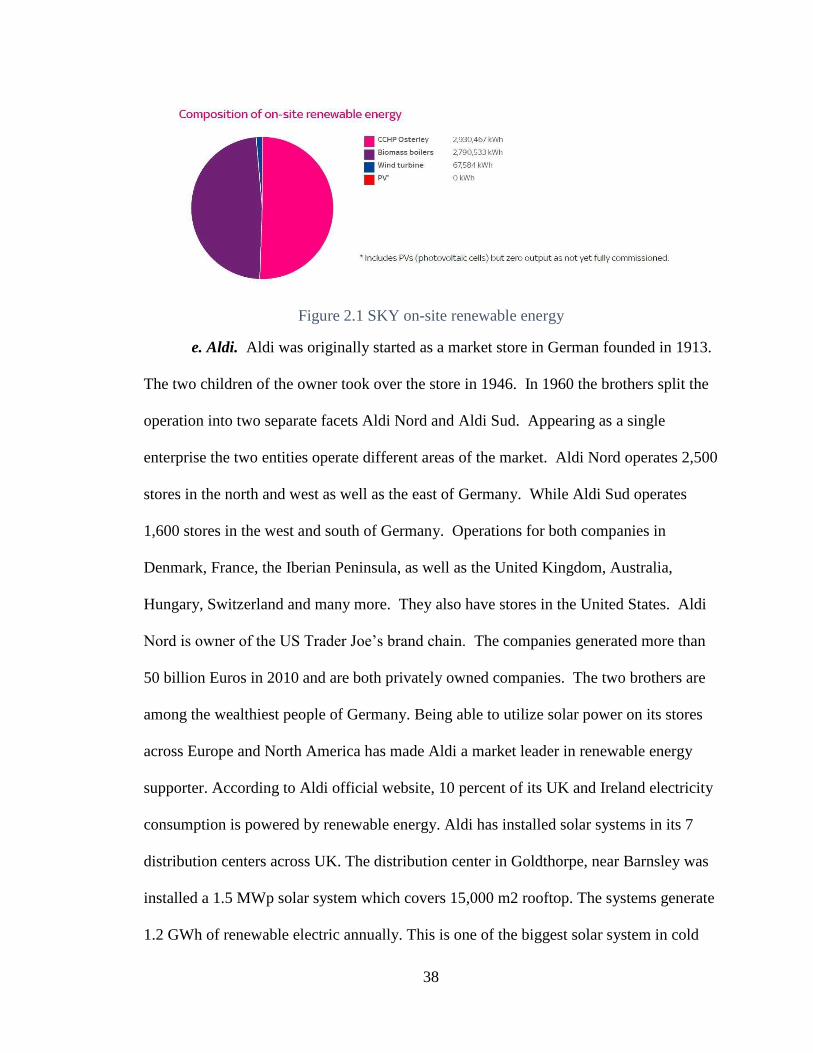
38
Figure 2.1 SKY on-site renewable energy
e. Aldi. Aldi was originally started as a market store in German founded in 1913.
The two children of the owner took over the store in 1946. In 1960 the brothers split the
operation into two separate facets Aldi Nord and Aldi Sud. Appearing as a single
enterprise the two entities operate different areas of the market. Aldi Nord operates 2,500
stores in the north and west as well as the east of Germany. While Aldi Sud operates
1,600 stores in the west and south of Germany. Operations for both companies in
Denmark, France, the Iberian Peninsula, as well as the United Kingdom, Australia,
Hungary, Switzerland and many more. They also have stores in the United States. Aldi
Nord is owner of the US Trader Joe’s brand chain. The companies generated more than
50 billion Euros in 2010 and are both privately owned companies. The two brothers are
among the wealthiest people of Germany. Being able to utilize solar power on its stores
across Europe and North America has made Aldi a market leader in renewable energy
supporter. According to Aldi official website, 10 percent of its UK and Ireland electricity
consumption is powered by renewable energy. Aldi has installed solar systems in its 7
distribution centers across UK. The distribution center in Goldthorpe, near Barnsley was
installed a 1.5 MWp solar system which covers 15,000 m2 rooftop. The systems generate
1.2 GWh of renewable electric annually. This is one of the biggest solar system in cold
39
store facility in UK in 2015. Furthermore, in 2015, Aldi installed a 2.1 MW solar panels
system on top of its regional distribution center in Boston, UK. This 8,240- panel system
generates approximately 1,746 MWh of renewable energy per year which can power six
time the electricity needed for the store annually. Early 2017, Aldi plans to install a 1.5
MWp system on its Cardiff distribution center which locates on the south coast of Wales.
Aldi stores in Germany has celebrate its 1000th PV systems installed on store rooftop.
The company states that renewable energy is used to cool the merchandise and for
lighting in more than half of its stores in western and southern Germany. The renewable
energy systems in Germany stores generates 95 million kWh which 85 percent is used to
supply cooling and lighting in the stores. The remaining 15 percent of renewable energy
is sent to the local grid.
f. M&S. M&S is the first retailer in the world that claims to have carbon neutral
operations. In 2009, M&S signed a contract with local renewable energy company to
supply its stores and offices in England and Wales by renewable energy for six years.
With the commitment to use 100 percent renewable energy for electricity demand, since
2012, all of its UK and Ireland stores, warehouse, offices are power by the renewable
energy came from green tariff renewable energy sources. 21 percent of its energy comes
from small scale generator such as wind farm and solar system by 2014. In 2015, M&S
joined RE 100 and targeted to use 100 percent of renewable energy globally and 50
percent from small scale renewable source by 2020. M&S also installed UK largest solar
panel array on its East Midlands distribution center in Castle Donington in 2014. The
solar system covers 900,000 sq. ft. roof and generate more than 5,000 MWh of renewable

40
energy annually. This system will provide 25 percent of energy needed by the distribution
center.
2.2.4 Service industry in Africa.
a. Woolworths. Woolworths is a national retailer located only in South Africa. It
was started in 1931 by Max Sonneberg and his son Richard. It famously made its debut
inside of the notable Royal Hotel. Since then it developed a business relation with Marks
& Spencer of London and shared a technology agreement that is still used today. Among
its products and services are food, clothing wear, financial services, and homeware. As
of 2016 it operated on 4billion US dollars and employed over 18,000 workers in South
Africa. Woolworths accomplished its sustainability goals for the 2007-2015 period and in
the process, could supply 10% or 254,369 kWh to its headquarters. Also, in 2014, it
purchased an amount of 200,000 kWh of Green Electricity certificates from the City of
Cape town. Throughout its stores it was able to reduce 40% of relative electricity used as
well as 31% in its corporate structures. It is currently planning on creating a 2MW solar
array at its Midrand distribution center that would have the capacity to power up to 34%
of the total energy needed annually. Woolworths in accordance with its commitment has
set new goals to reduce its current energy use by halve in 2020 and be completely energy
independent by 2030.
b. Massmart Holdings Limited. Massmart is one of South Africa’s biggest
retailer being the biggest wholesaler of basic food items as well as general merchandise.
It was started in 1990 with the acquisition of six Makro stores in the country and has
grown ever since. It operates under several divisions including a Masswarehouse and
Massbuild which includes Builders Warehouse and Makro. Walmart in 2010 acquired a

41
51% share in its stock and is now the parent company. As of 2014 it operated on a net
revenue of 3billion dollars US and employed more than 45,000 workers. Currently
Massmart has over shot their goal of being 10% energy efficient and reached 18.76%
energy efficiency throughout their operations. It is currently spearheading three
renewable resources the first which is a 150kva Photovoltaic source which will operate in
its Builders Warehouse store. It has a 700kva plant for one of its Makro stores and
520kva for another Makro store in Carnival Mall. Massmart is also a supporter of energy
efficiency initiatives sponsored by South Africa’s National Business Initiative.
c. Pick n Pay Stores Limited. Pick n Pay is an international supermarket store
centered in South Africa which was founded in 1967. The company underwent a
complete redesign which had been mostly unchanged since the 1970’s. The company
operates on revenue of 4 billion US dollars and employs 50,000 employees. Currently
Pick n Pay is under plans to install a 300kWp solar array at its distribution center in
Western Cape. It has already installed a 150kWp array in its Longsmeadow distribution
center and there is a 100kWp solar array at its Hurlingham store. Its energy per square
meter use has been reduced by 32% since 2008 and is now retrofitting one of its stores to
test the viability for further use throughout its operations.

42
III.WIND TURBINE AND PV CAPACITOR MODEL AND ELECTRIC
VEHICLE ENERGY INTENSITY
3.1. Wind Turbine Capacitor Factor
A wind turbine (WT) system possesses four operating phases depending on the
wind speed. Let Pw(v) be the instantaneous output of wind turbine at wind speed v. Then
the cubic power curve is given as (Thiringer and Linders, 1993).
=
srm
rcrm
sc
w
vvvP
vvvvvP
vvvv
vP 3)/(
,0
)( (3.1)
where vc, vr and vs stands for the cut-in speed, the rated speed, and the cut-off speed
respectively. Note Pm is the rated power capacity in a unit of either MW or KW
depending on the size of the wind turbine. Studies (Weekes and Tomlin 2014) have
shown that the wind speed in a particular location in general can be fitted with Weilbull
distribution. The probability density function (PDF) and cumulative distribution function
(CDF) are given below
kcv
k
w ec
v
c
kvf )/(
1
)( −
−
= , for v0 (3.2)
kcv
w evF )/()( −= , for v0 (3.3)
where c and k are the Weibull scale and shape parameters. Then the WT capacity factor,
denoted as w can be estimated as
( ))()()(1)]([ 3
3 rwsw
v
v
w
rm
ww vFvFdyyfy
vTP
TVPE r
c
−+=
= (3.4)
where T is the number of hours in a year. The value of w falls in the range of [0, 1]. An
example of Weibull wind speed distribution is in Figure 3.1
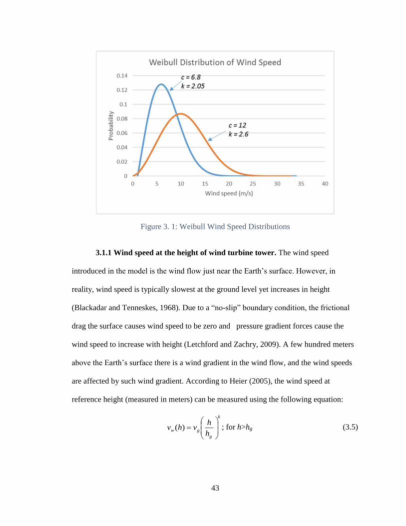
43
Figure 3. 1: Weibull Wind Speed Distributions
3.1.1 Wind speed at the height of wind turbine tower. The wind speed
introduced in the model is the wind flow just near the Earth’s surface. However, in
reality, wind speed is typically slowest at the ground level yet increases in height
(Blackadar and Tenneskes, 1968). Due to a “no-slip” boundary condition, the frictional
drag the surface causes wind speed to be zero and pressure gradient forces cause the
wind speed to increase with height (Letchford and Zachry, 2009). A few hundred meters
above the Earth’s surface there is a wind gradient in the wind flow, and the wind speeds
are affected by such wind gradient. According to Heier (2005), the wind speed at
reference height (measured in meters) can be measured using the following equation:
k
g
gwh
hvhv
=)( ; for h>hg (3.5)

44
Where vw(h) is the velocity of the wind (m/s) at height h. Velocity of the wind at
height hm (m) is denoted at vm (m/s). The parameter k is the Hellman exponent that
depends on the coastal location and the shape of the terrain on the ground, and the
stability of the air. Table 3.1 provides example values of the Hellmann exponent. This
research uses the unstable air above human inhabited areas k= 0.27.
Table 3. 1 Hellmann Exponent
Location k
Unstable air above open water surface 0.06
Neutral air above open water surface 0.1
Unstable air above flat open coast 0.11
Neutral air above flat open coast 0.16
Stable air above open water surface 0.27
Unstable air above human inhabited areas 0.27
Neutral air above human inhabited areas 0.34
Stable air above flat open coast 0.4
Stable air above human inhabited areas 0.6
3.2. Solar PV Capacitor Factor (in Northern Hemisphere)
The output power of a PV system depends on multiple factors that are
summarized in Table 3.2. Unless specified, the unit of all angles is radians (rad).

45
Table 3. 2: Key Parameters in Solar PV Power Generation
No. Factor Symbol Explanation
1 weather condition Wt random variable
2 PV size (m2) A PV module area
3 PV efficiency 10-20% for commercial PV
4 calendar date d d{1, 2, …, 365}
5 solar hour (rad) related to the local time
6 PV temperature (oC) To operating temperature
7 latitude (rad) depends on location
8 PV azimuth angle (rad) if facing south
9 PV tilt angle (rad) between PV and ground
10 Solar zenith angle (rad) between the zenith and the Sun’s ray
11 solar PV incident angle Between the norm to PV and the Sun’s ray
12 local hours t t=1, 2, …, 24
We present a three-step procedure to calculate the PV power output based on the
early studies in (Cai et al. 2010). These steps are summarized as follows
Step 1: For PV facing the south, the sunrise and sunset time in day d{1, 2, …, 365}
tan)tan()cos()cos( −−==− setrise (3.5)
with
+=
365
)284(2sin40928.0
d (3.6)

46
where, is the declination angle, rise and set are the sunrise and the sunset angles in day
d perceived from the PV panel. There is no power output before sunrise and after sunset.
Step 2: Computing the total solar irradiance incident on the PV surface at time t on date d
( )
−+
−+=
−
11.0cos365
)4(2cos034.017.01370
678.0)(cos dI t (3.7)
where
sinsincoscoscoscos += (3.8)
sinsinsincoscoscossinsincos
coscoscoscoscossincossincossinsincos
++
+−= (3.9)
In Equation 3.7, It is the solar irradiance (W/m2) received by the PV under a clear
sky condition and is the solar zenith angle given by Equation (3.8) and it is the angle
between the zenith and the center of the Sun. is the solar hour angle determined by
time t. For instance, =0 is the solar noon time. Starting from =-/2 at 6am, and doing
increases of 15 degrees every hour until reaching =/2 at 6pm. To maximize the energy
yield, the PV panel faces the South and its tilt angle shall equal the local latitude, namely
=0 and =, then equation (3.9) can be simplified as
coscoscos = (3.10)
Step 3: The actual output of a PV system considering the uncertain weather condition
can be estimated as
)25(005.01 −−= ottt TAIWP (3.11)
where Pt is the actual output power (unit: W) of the PV system at time t. Wt is a random
variable representing the stochastic weather at time t. It varies from 1 and 0 to mimic a
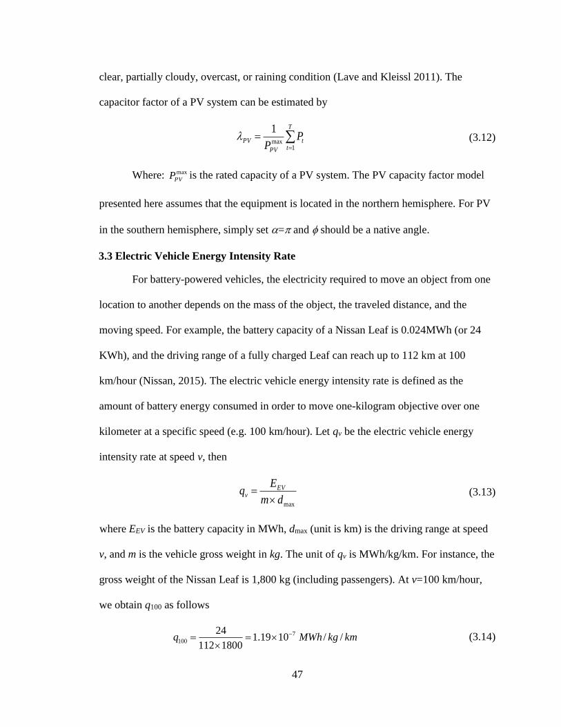
47
clear, partially cloudy, overcast, or raining condition (Lave and Kleissl 2011). The
capacitor factor of a PV system can be estimated by
=
=T
tt
PV
PV PP 1
max
1 (3.12)
Where: max
PVP is the rated capacity of a PV system. The PV capacity factor model
presented here assumes that the equipment is located in the northern hemisphere. For PV
in the southern hemisphere, simply set = and should be a native angle.
3.3 Electric Vehicle Energy Intensity Rate
For battery-powered vehicles, the electricity required to move an object from one
location to another depends on the mass of the object, the traveled distance, and the
moving speed. For example, the battery capacity of a Nissan Leaf is 0.024MWh (or 24
KWh), and the driving range of a fully charged Leaf can reach up to 112 km at 100
km/hour (Nissan, 2015). The electric vehicle energy intensity rate is defined as the
amount of battery energy consumed in order to move one-kilogram objective over one
kilometer at a specific speed (e.g. 100 km/hour). Let qv be the electric vehicle energy
intensity rate at speed v, then
maxdm
Eq EV
v
= (3.13)
where EEV is the battery capacity in MWh, dmax (unit is km) is the driving range at speed
v, and m is the vehicle gross weight in kg. The unit of qv is MWh/kg/km. For instance, the
gross weight of the Nissan Leaf is 1,800 kg (including passengers). At v=100 km/hour,
we obtain q100 as follows
kmkgMWhq //1019.11800112
24 7
100
−=
= (3.14)
48
For instance, to move a 4,000-kg object over 100 km at a speed of 100 km/hour,
the amount of electricity consumed is q100×4,000×100=0.04762 MWh. The driving
distance of fully charged electric truck is typically in a range between120 and 160 km
(Daclison-Dickey, 2013). Hence battery charging stations along the traveling route is
required to accommodate the e-truck transportations beyond the driving range.

49
IV. NET ZERO CARBON MANUFACTURING FOR SINGLE FACILITY PLUS
WAREHOUSE AND E-TRANSPORT -DETERMINISTIC DEMAND
4.1 Systems and Model Settings
4.1.1 Design setting. In this phase of the research, we consider a single
manufacturing site and a warehouse network with electric truck (e-truck) as a sole
transportation tool to ship products between two facilities. The energy needed to perform
regular operations for these two facilities are provided by the onsite renewable energy
generation systems. Two types of renewable generators are considered for this research
which include wind turbine (WT) and photovoltaic (PV). Furthermore, the e-vehicle also
use the onsite renewables to charge its battery. The goal of this study is to create the net
zero carbon emission manufacturing-warehouse zone.
Figure 4. 1: A single facility and warehouse setting with onsite generation
The ideal model is to produce enough energy using onsite generation to supply
the electricity demand for the facilities. However, the output of WT and PV will be
uncertain due to stochastic weather conditions thus will occasionally create energy
shortage and surplus. To meet the needs of the energy usage during the shortage period,
where the output of renewable energy is less than the demand, the plant will use the
energy imported from the main grid. On the other hand, in the scenario of surplus, where
50
the onsite energy generated is more than the consumption, it can be fed back to the main
grid. Net metering or feed-in-tariff are the current two mechanisms that faceplate the
onsite generation system to exchange the renewable energy with the main grid. This
practice will maintain the net zero carbon emission of the network as the shortage energy
borrowed from the grid is offset with the surplus energy sent to the main grid.
4.2 Optimization Algorithm
4.2.1. Production-inventory model. A production inventory model is considered
where multiple products are produced in a single factory over multiple periods. Each item
has a bill of materials described by its production cost, inventory cost, and backorder
cost. Based on the following notation, the mathematical model for a linear multiple
period production inventory model is formed.
xij : decision variable for quantity of product type i made in period j
yij : decision variable for inventory level of product type i in period j
zij : decision variable for backorder level of product type i in period j
oij : cost for producing a unit of product type i in period j
hij : cost for holding a unit of product type i in period j
bij : cost for backordering a unit of product type i in period j
Dij : demand rate of product type i in period j
vis : amount of resource s consumed for making a unit of product type i
wsj : total availability of resource s in period j
With the three decision variables xij, yij, and zij, the mathematical model is formed to
determine the optimal values of the production, inventory, and backorder level that meet
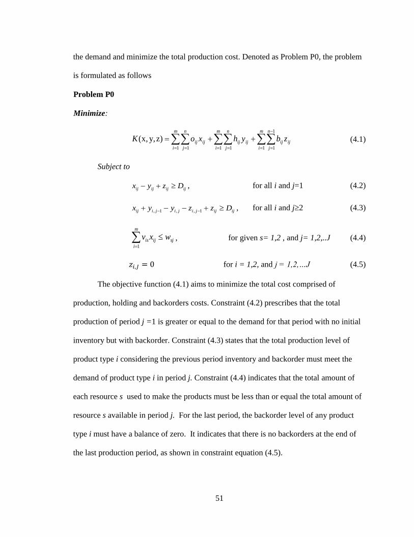
51
the demand and minimize the total production cost. Denoted as Problem P0, the problem
is formulated as follows
Problem P0
Minimize:
=
−
== == =
++=m
i
n
j
ijij
m
i
n
j
ijij
m
i
n
j
ijij zbyhxoK1
1
11 11 1
)z,y,x( (4.1)
Subject to
ijijijij Dzyx +− , for all i and j=1 (4.2)
ijijjijijiij Dzzyyx +−−+ −− 1,,1,, for all i and j2 (4.3)
sj
m
i
ijis wxv =1
, for given s= 1,2 , and j= 1,2,..J (4.4)
𝑧𝑖,𝐽 = 0 for i = 1,2, and j = 1,2,…J (4.5)
The objective function (4.1) aims to minimize the total cost comprised of
production, holding and backorders costs. Constraint (4.2) prescribes that the total
production of period j =1 is greater or equal to the demand for that period with no initial
inventory but with backorder. Constraint (4.3) states that the total production level of
product type i considering the previous period inventory and backorder must meet the
demand of product type i in period j. Constraint (4.4) indicates that the total amount of
each resource s used to make the products must be less than or equal the total amount of
resource s available in period j. For the last period, the backorder level of any product
type i must have a balance of zero. It indicates that there is no backorders at the end of
the last production period, as shown in constraint equation (4.5).

52
4.2.2. Cost model of onsite generation system.
a. Installation cost. Cin(Pc) stands for the annualized installation cost for the
onsite renewable energy distribution grid (DG) with Pcg is generation type g capacity
==
=−+
+=
G
g
c
gkg
G
g
c
ggn
nc
in PaPar
rC
111)1(
)1()P(
(4.6)
where ag is the capacity cost per MW of generation type g. The capital recovery
factor, , is given by where n is the number of years to pay
the equipment loan, and r is the interest rate, note that r = 0.05.
b. Operating and maintenance cost. As mentioned above, this research considers
two types of renewable energy: wind and solar power. Even though these natural
resources are accessible, the companies still incur in the following costs: (1) leasing land
to install the WT, PV, and accessory units; and (2) replacement or repair of worn out
components due to aging. Operation and maintenance (O&M) cost correlate with the cost
of equipment usage and system monitoring. Com(Pc) stands for the annual DG operating
and maintenance (O&M) cost which is given as follows.
= =
=J
j
G
g
c
gjkgjkgg
c
om PbC1 1
)P( (4.7)
where Pgjk is the actual output of generation type g during period j at location k, bg is the
average O&M cost in producing 1 MWh electricity by generation type g, and gjk is the
capacity factor of generation type g for the period j at location k. Let τg be the operation
hours per year for generation type g. Equation 4.7 assumes the sun is above the
horizontal 50 percent of the time for a standard year of 8760 hours. Thus, the maximum
daytime hours of sun will be 4380 hours for any point on Earth (τPV = 4,380 hours). On
]1)1/[(])1([ −++= nn rrr

53
the other hand, the maximum wind duration per year will be 8760 hours at any point on
Earth (τWT = 8760), though its speed varies.
c. Carbon credit. Various incentive programs are proposed by various
governments around the world to stimulate the investment in wind and solar energy.
Among the most popular ones are carbon credits and equipment subsidies. The last ones
are offered as one-time carbon credits to the renewable energy producer. Ccr(Pc)
represents the annual carbon credits for the manufacturing facility where
= =
=J
j
G
g
c
gjkgjkgg
c
cr PcC1 1
)P( (4.8)
Let cg be the carbon credits ($/MWh) for renewable energy type g. If the incentive
program or the subsidy policy for a specific generation type g has expired, this model can
be flexible by simply setting cg = 0 for that particular renewable technology.
4.2.3. Net zero carbon manufacturing for single factory plus warehouse and e-
transport. Based on the above production inventory model and generation system cost
model, a new mathematical model is formed to determine the appropriate system capacity
to install in the factory and warehouse location to meet the production demand as well as
minimize the annual total cost of operation. Problem’s notations are listed in table below.

54
Table 4. 1 The Notation for the Problem
Notation Explanation
P1kc wind turbine capacity at location k (k=1 is the manufacturing
facility and k=2 is the warehouse, decision variable
P2kc PV capacity at location k (k=1 is the manufacturing facility
and k=2 is the warehouse), decision variable
xij quantity of product i made in period j, decision variable
yij inventory of product i in period j, decision variable
zij backorder of product i in period j, decision variable
oij cost for producing unit i in period j
hij cost for holding unit i in period j
bij cost for backordering unit i in period j
ij transportation cost for unit i in period j
Dij demand for product i in period j
vis the amount of resource s consumed for making unit i
wsj total available resource of s in period j
q the electric transport energy intensity rate
wp the payload per trip between factory and warehouse
wv the vehicle self-weight per trip factory and warehouse
d the distance between factory and warehouse
n the number of yearly trips between factory and warehouse
number of hours in a year
ag capital cost for renewable energy type k
bg operation and Management cost for renewable energy type k
cg carbon credits for renewable energy type k
ʎgjk capacity factor of month j and renewable energy type g at
location k
ei energy consumed for each product type i
E energy consumed by the warehouse
h warehouse operation hours
CDG Total cost of the distributed generation system

55
Mathematical model
Problem P1
Minimize:
)P,x()()P,z,y,x(1
1
11 11 1
c
DG
m
i
n
j
ijij
m
i
n
j
ijij
m
i
n
j
ijiij
c Czbyhxuof ++++= =
−
== == =
(4.9)
Where = == ==
−+=J
j
G
g
c
gjkgjkgg
J
j
G
g
c
gjkgjkgg
G
g
c
gkgDG PcPbPaC1 11 11
(4.10)
Subject to:
ijijijij Dzyx +− , for all i and j=1 (4.11)
ijijjijijiij Dzzyyx +−−+ −− 1,,1,, for all i and j2 (4.12)
sj
m
i
ijis wxv =1
, for given s= 1,2 , and j= 1,2,..J (4.13)
𝑧𝑖,𝐽 = 0 for i = 1,2, and j = 1,2,…J (4.14)
====
=++G
g
c
gjgj
J
j
g
vpJ
j
iij
I
i
Pwwqndex1
,1,1
111
)(
(4.15)
hE + 𝑞𝑛𝑑(𝑤𝑣) = ==
G
g
c
gjgj
J
j
g P1
,2,2
1
(4.16)
.0c
gjkP , xij, yij, zij ≥ 0 (4.17)
In equation (4.9), it can be observed that if renewable energy is allowed to
increase, more compensation will return to the company. Constraint (4.15) indicates that
the total energy generated by the renewable energy system needs to be balanced with the
total energy consumed by the manufacturing and the electrical vehicle at each month j

56
and renewable energy type g . Let wv be the weight of empty vehicle while wp is the
weight of each product transported. In this constraint, q is the transport energy intensity
rate. Constraints (4.16) prescribes the total energy produced by onsite generation shall be
equal to the total energy consumed by the warehouse and the e-vehicles where h is the
yearly operation hours of the warehouse and E is power consumed by the warehouse. The
last constraint (4.17) states that all the decision variables are non-negative and the
production, inventory, and backorders variables are integer.
4.3. Climate Data
The generation WT and PV systems rely on the geographic location of the
facilities to sustain the energy required for operation. Since the weather is unpredictable
and impossible to control, the study of weather profile history is suggested to forecast the
future seasonal weather conditions of specific locations.
For accurate analysis of the weather pattern, a data range of eleven years is
utilized in the model. In order to demonstrate the varying types of climate conditions, the
weather profiles are divided into different categories such as clear day, scattered cloud
(SC), partially cloudy (PC), mostly cloudy(MC), overcast, rain, fog, storm/T-storm and
snow. The average daily wind velocity in m/s is also gathered for a period range of
eleven years. All the information about the weather conditions and wind speeds are
retrieved from Weather Underground web portal (WU 2017). To demonstrate the
previous conditions, two cities for each significant weather condition were selected due
to their relative location from each other and their dramatic weather conditions.
4.3.1 Large wind locations. Voted as the world windiest city, Wellington is the
best choice to test the model under large wind conditions. Wellington is the capital of

57
New Zealand with the second largest population in New Zealand. Located at the Roaring
Forties and receive the wind blow from Cook Strait, it made Wellington become the
windiest place in the world with the average wind speed of 7 m/s above the ground
surface. Figure 4.2 is the histogram of Wellington weather conditions in 2016. Figure 4.3
presents the wind speed data for this city at a height of 80 meters.
Figure 4. 2: Wellington Weather Condition in 2016
Figure 4. 3: Wellington Average Wind Speed at the Height of 80 Meters
12
144
16 17
165
4 2 0 3 20
20406080
100120140160180
DA
Y
WEAHTER CONDITION
Wellington Weather Condition
0
2
4
6
8
10
12
14
16
18
20
1 3 5 7 9 11 13 15 17 19 21 23 25 27 29 31 33 35 37 39 41 43 45 47 49 51
Win
d S
pee
d (
m/s
)
Week
Wellington Average Wind Speed

58
Christchurch is located at the South Island of New Zealand and it is the largest
city in the South. Located more than 500 kilometers south of Wellington, Christchurch is
the third largest city in New Zealand, behind Auckland and Wellington. Below is the
histogram of Christchurch weather conditions in 2016.
Figure 4. 4: Weather conditions of Christchurch in the 2016
4.3.2 Strong sun. The city of Aswan is an ideal location to test the model under
mostly sunny weather conditions. Aswan is a city located in the south of Egypt, on the
first bank of the Nile River. Aswan is known as one of the sunniest cities in the world.
Average high temperature is steadily about 40 degrees in Celsius (104 oF) where the
average low temperature is about 25 degrees in Celsius (77 oF)). Figures 4.5 and 4.6 are
the histograms demonstrating the weather conditions and wind speed of Aswan in the
year 2016, respectively.
36
66
1529
143
6
65
1 2 20
20406080
100120140160
DA
Y
WEATHER CONDITION
Christchurch Weahter Condition
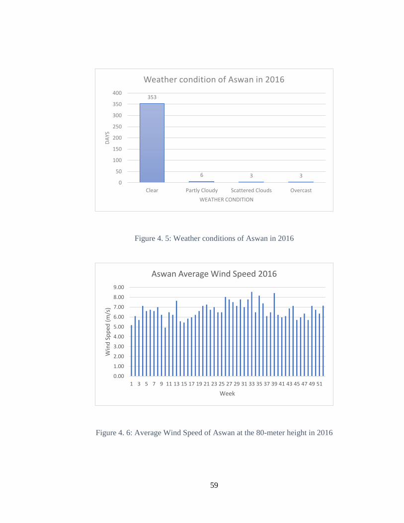
59
Figure 4. 5: Weather conditions of Aswan in 2016
Figure 4. 6: Average Wind Speed of Aswan at the 80-meter height in 2016
353
6 3 30
50
100
150
200
250
300
350
400
Clear Partly Cloudy Scattered Clouds Overcast
DA
YS
WEATHER CONDITION
Weather condition of Aswan in 2016
0.00
1.00
2.00
3.00
4.00
5.00
6.00
7.00
8.00
9.00
1 3 5 7 9 11 13 15 17 19 21 23 25 27 29 31 33 35 37 39 41 43 45 47 49 51
Win
d S
pp
ed (
m/s
)
Week
Aswan Average Wind Speed 2016

60
The city of Luxor in Egypt is chosen due to its convenient location in southern
Egypt (Upper Egypt) along the Nile river. Luxor is 239 km south of Asswan. Luxor has a
similar climate as Asswan as it is also one of the sunniest city in the world. The city is
one of the driest place on the Earth where rainfall does not occur very often. Average
temperature of Luxor is between 22 oC (72 oF) and 40 oC (104 oF). Figures 4.7 and 4.8
are the histograms demonstrating the weather conditions and wind speed profile of Luxor
in year 2016.
Figure 4. 7: Weather conditions of Luxor in 2016
333
18 9 2 30
50
100
150
200
250
300
350
Clear PartlyCloudy
ScatteredClouds
Rain Overcast
DA
YS
WEATHER CONDITION
Weather condition of Luxor in 2016

61
Figure 4. 8: Average Wind Speed of Luxor at the 80-meter height in 2016
4.3.3 Mix of large wind and strong sun. Yuma is located in the southwestern
part of Arizona state. The city is known for its extreme weather pattern which features a
hot desert climate. Yuma is the driest and sunniest city in the United States with annual
average possible sunshine of 90 percent according to National Oceanic and Atmospheric
Administration. The histogram graphs in Figures 4.9 and 4.10 illustrate the weather and
wind conditions of Yuma in the year of 2016, respectively.
0
1
2
3
4
5
6
7
8
1 3 5 7 9 11 13 15 17 19 21 23 25 27 29 31 33 35 37 39 41 43 45 47 49 51
Win
d S
pee
d (
m/s
)
Week
Luxor Average Wind Speed 2016

62
Figure 4. 9: Weather Condition of Yuma in 2016
Figure 4. 10: Average Wind Speed of Yuma at the 80-meter height in 2016
San Francisco is a popular tourist destination in the U.S. Located in the north end
of San Francisco Peninsula. It is known for its cool summers and diverse mix of
163
73
102
0
16
0 0 010
0
20
40
60
80
100
120
140
160
180
Clear PartlyCloudy
ScatteredClouds
MostlyCloudy
Rain Overcast Fog Snow Tstorm
Day
Weather Condition
Weather Condition in 2016
0
2
4
6
8
10
12
1 3 5 7 9 11 13 15 17 19 21 23 25 27 29 31 33 35 37 39 41 43 45 47 49 51
Win
d S
pee
d (
m/s
)
Week
Average Wind Speed in 2016

63
architecture and landmarks. The climate of San Francisco is classified as Mediterranean
Climate with dry, sunny, and warm summer while the weather condition in the winter is
mild, wet, and occasionally stormy. The weather and wind conditions of San Francisco in
2016 are demonstrated in the Figures 4.11 and 4.12 below.
Figure 4. 11: Weather Condition of San Francisco in 2016
14
162
100
14
70
0 4 0 10
20
40
60
80
100
120
140
160
180
DA
Y
WEATHER CONDITION
Weather Condition in 2016

64
Figure 4. 12: Average Wind Speed of San Francisco at the 80-meter height in 2016
Weather conditions and wind speed for each city are collected to obtain historical
data and capture a long range of climate conditions. In total, there are 4,015 daily wind
speed measurements for each city and an overall total of 32,120 wind speed samples will
be used to estimate the WT capacity factor for the model. Similarly, the daily weather
conditions for each city are also collected with total of 4,015 data points for each city and
a total of 32,120 observations for the time frame from 2006 to 2016 for the eight cities
that are used in the model. The size of the data set used for the model is 64,240 data
points. The average wind speed and weather conditions of six cities are demonstrated in
Table 4.2 below.
0
2
4
6
8
10
12
14
16
18
1 3 5 7 9 11 13 15 17 19 21 23 25 27 29 31 33 35 37 39 41 43 45 47 49 51
Win
d S
pee
d m
/s
Week
Average Wind of 2016

65
Table 4. 2: Average Wind Speed and Weather Conditions of Six Cities
Country New Zealand Egypt USA
City Wellington Christchurch Aswan Luxor Yuma San
Francisco
Latitude (Deg) 41.29 43.53 24.09 25.69 32.69 37.77
Ground AWS 6.71 3.84 5.93 1.44 2.97 4.05
Ground SWS 2.91 1.77 2.29 0.67 1.4 1.83
Clear days 6 20 356 337 165 28
Scattered Cloud 68 41 5 11 109 95
Partially Cloudy 109 98 3 14 65 136
Mostly Cloudy 5 11 0 0 0 13
Overcast 1 3 0 1 0 2
Rain 170 131 0 1 13 65
Fog 2 56 0 0 1 24
Storm/T-Storms 3 3 0 0 11 3
Snow 0 3 0 0 0 0
Note: AWS=average wind speed (m/s), SWS=standard deviation of wind speed (m/s).
As observed from the table, Wellington has strong wind velocity with AWS of
6.71 m/s, yet it only has 6 clear days. On the other hand, Luxor has 337 clear days but the
average wind speed (AWS) is only 1.44 m/s. San Francisco has medium wind speed with
AWS of 4.05 m/s and it has 28 clear days. Since the wind speeds and weather conditions
of eight cities are diverse, they can represent the areas where most of the human beings
reside.
4.3.4 Estimating capacity factor of wind turbine. Wind speed data shown in
Table 4.3 usually are recorded and provided by the Automated Surface Observing
Systems (ASOS) of the local airport which is often placed at 8-10 meters above the
ground. However, we need to consider the height of the wind turbine to accurately
calculate the turbine capacity factor. Using Hellmann exponent k=0.27 and the equation
to calculate wind speed at specific height, mentioned in Section 3.1 (Chapter 3), the wind

66
speed at h= 80 meter height would be vw(80)=vg(80/10)0.34=2.03vg. This is twice of the
wind speed at hg=10 m.
Table 4. 3: Wind Speed of Week 1 in Wellington (unit: m/s)
Day 2016 2015 2014 2013 2012 2011 2010 2009 2008 2007 2006
10-m
above
ground
1 2.7 5.8 8.5 8.9 7.6 5.4 9.4 8.5 2.7 11.6 3.6
2 4.0 5.8 8.5 12.5 6.7 8.9 11.6 8.5 7.2 11.6 10.7
3 7.6 6.3 12.5 9.8 5.4 8.9 8.1 9.8 11.1 8.9 9.8
4 11.6 6.3 9.4 4.0 6.3 8.1 9.4 4.5 6.3 3.6 10.2
5 2.7 10.2 8.9 3.6 11.1 5.8 5.4 7.6 4.5 8.9 5.4
6 4.0 6.7 7.6 5.8 8.1 5.8 10.7 10.7 8.5 12.5 4.5
7 8.9 4.9 10.2 7.6 6.3 10.7 12.0 11.1 8.9 5.4 7.6
80-m
tower
1 4.7 10.1 14.8 15.6 13.3 9.4 16.4 14.8 4.7 20.3 6.3
2 7.1 10.2 14.9 21.9 11.8 15.7 20.4 14.9 12.5 20.4 18.8
3 13.3 11.0 21.9 17.2 9.4 15.7 14.1 17.2 19.6 15.7 17.2
4 20.4 11.0 16.5 7.1 11.0 14.1 16.5 7.8 11.0 6.3 18.0
5 4.7 18.0 15.7 6.3 19.6 10.2 9.4 13.3 7.8 15.7 9.4
6 7.1 11.8 13.3 10.2 14.1 10.1 18.8 18.8 14.9 22.0 7.8
7 15.7 8.6 18.0 13.3 11.0 18.8 21.2 19.6 15.7 9.4 13.3
The wind speed data for the first week of Wellington city are used to demonstrate
how to estimate the capacity factor (CF) of WT. The first section of the table lists the
daily ground wind speed in Wellington between 2006 and 2016. Assuming k=0.27, the
corresponding wind speed in 80-m height is calculated and the results are shown in the
second section of the table. The typical height of a WT tower of 1.5 - 2.5 MW capacity is
80 meters. Figure 4.13 plots the weekly wind turbine CF for all the eight cities based on
the 2.5 MW WT installation.

67
Figure 4. 13: Weekly Wind Turbine Capacity Factor of Eight Cities
4.3.5 Estimating capacity factor of solar PV. The daily weather conditions
retrieved from the WU portal are broken down into eight states as clear, rain, partial
cloud, scatter cloud, mostly cloudy, fog/storm, overcast, and snow. For illustration
purposes, Table 4.4 lists the daily weather state of Week 1 in Wellington between 2006
and 2016.
Table 4. 4: Daily Weather Condition from 2006 to 2016 in Wellington
Day 2016 2015 2014 2013 2012 2011 2010 2009 2008 2007 2006
1 Clear PC Rain SC Rain PC SC SC SC Rain PC
2 Rain SC PC PC Rain SC PC Rain SC Rain Rain
3 Rain Rain Rain SC PC SC Rain Rain PC PC Rain
4 Rain PC Rain SC SC PC Rain SC PC SC Rain
5 Clear PC Rain Clear PC Fog SC SC SC PC Rain
6 PC MC PC PC PC Rain PC PC Rain PC Rain
7 PC Rain PC PC PC PC PC PC Rain PC PC
Based on the daily weather conditions, the number of days with a particular state can be
counted, and the results are summarized in the last row in Table 4.5. For instance, the
0.0
0.1
0.2
0.3
0.4
0.5
0.6
0.7
0.8
0.9
0 5 10 15 20 25 30 35 40 45 50
WT
Capacit
y F
acto
r
Week
Wellington Christchurch Aswan Luxor
Yuma San Francisco El Paso Phoenix

68
total number of “Clear” days for Week 1 in Wellington is 3 over eleven years, and the
total number of “Rain” days is 25. For a given day in that week, the probability of a
particular weather state now can be estimated. For instance, the probability of a “Clear”
day is 3/77=0.04, and the probability of “PC” is 31/77=0.4. These probabilities are used
to simulate the PV generation for Week 1 in Wellington.
Table 4. 5: The Probabilities of Weather States for Week 1 in Wellington
Day Clear SC PC MC OC Rain Fog/Storm Snow
1 1 4 3 0 0 3 0 0
2 0 3 3 0 0 5 0 0
3 0 2 3 0 0 6 0 0
4 0 4 3 0 0 4 0 0
5 2 3 3 0 0 2 1 0
6 0 0 7 1 0 3 0 0
7 0 0 9 0 0 2 0 0
Sum 3 16 31 1 0 25 1 0
Probability 0.04 0.21 0.40 0.01 0.00 0.32 0.01 0.00
Under the clear sky condition, the solar irradiance incident on PV surface,
denoted as It (W/m2), can be precisely estimated. The detailed steps to estimate It are
provided in Chapter 3. The random output of PV is primarily caused by the uncertain
weather states. To estimate the solar irradiance in different weather states, the weather
coefficient Wt is introduced to quantifying the actual amount of It incident on the PV
surface. For instance, if it is “Clear”, Wt=1, meaning the PV receives 100 percent of It. If
it is “PC,” then only 50 percent of It reaches the PV surface. In a snowy day, Wt=0
because the PV surface is likely to be covered by snows. The values of Wt corresponding
to different weather states are listed in Table 4.6. Now the actual PV generation can be
estimated based on the PV capacity formula in Section 3.2 (Chapter 3).
Table 4. 6: Weather Coefficients under Different States
No. 1 2 3 4 5 6 7 8
State Clear SC PC MC Overcast Rain Fog/Storm Snow
Wt 1 0.7 0.5 0.3 0.2 0.1 0.1 0
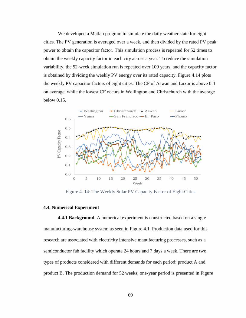
69
We developed a Matlab program to simulate the daily weather state for eight
cities. The PV generation is averaged over a week, and then divided by the rated PV peak
power to obtain the capacitor factor. This simulation process is repeated for 52 times to
obtain the weekly capacity factor in each city across a year. To reduce the simulation
variability, the 52-week simulation run is repeated over 100 years, and the capacity factor
is obtained by dividing the weekly PV energy over its rated capacity. Figure 4.14 plots
the weekly PV capacitor factors of eight cities. The CF of Aswan and Luxor is above 0.4
on average, while the lowest CF occurs in Wellington and Christchurch with the average
below 0.15.
Figure 4. 14: The Weekly Solar PV Capacity Factor of Eight Cities
4.4. Numerical Experiment
4.4.1 Background. A numerical experiment is constructed based on a single
manufacturing-warehouse system as seen in Figure 4.1. Production data used for this
research are associated with electricity intensive manufacturing processes, such as a
semiconductor fab facility which operate 24 hours and 7 days a week. There are two
types of products considered with different demands for each period: product A and
product B. The production demand for 52 weeks, one-year period is presented in Figure
0.0
0.1
0.2
0.3
0.4
0.5
0.6
0 5 10 15 20 25 30 35 40 45 50
PV
Cap
acit
y F
acto
r
Week
Wellington Christchurch Aswan Luxor
Yuma San Francisco El Paso Phonix

70
4.15. Parameters associated with production, inventory, backorder and transportation
logistics are shown in Table 4.7.
Figure 4. 15: Production Demand of Product A and Product B
Table 4. 7: Production, Inventory, Backorders, Logistics and Energy Data
Comments Notation
Product
A (i=1)
Product B
(i=2) Unit
Energy consumed ei 0.9 1.2 MWh/unit
Production cost (w.o.* energy) pi 400 600 $/unit
Holding cost hi 80 120 $/period/unit
Backlog cost bi 150 250 $/unit
Shipping cost (no EV recharge) i 10 15 $/unit
Shipping cost (with EV
recharge) i 14 19 $/unit
Labor hours/item vi1 16 24 hours/unit
Machine hours vi2 100 200 hours/unit
Weight (including package) mi 3 4 Kg/unit
Mean demand ijD 1000 600 units/period
Standard deviation ijD 120 50 units/period
*w.o.=without
0
200
400
600
800
1000
1200
1400
1 3 5 7 9 11 13 15 17 19 21 23 25 27 29 31 33 35 37 39 41 43 45 47 49 51
Qu
anti
ty
Week
Production Demand
Product A Product B

71
Table 4. 8: Machine and Labor Resources in the Factory
Week
Labor
Resource
(hours)
Machine or
Tool Resource
Hours
Week
Labor
Resource
(hours)
Machine or Tool
Resource (Hours)
1 38,516 278,847 27 37,860 279,542
2 34,429 244,299 28 39,153 281,016
3 33,472 239,044 29 32,345 237,514
4 34,210 248,699 30 34,562 249,292
5 36,680 261,478 31 36,814 263,851
6 36,660 269,935 32 35,001 251,627
7 34,063 249,447 33 32,159 239,152
8 35,786 261,961 34 37,138 269,049
9 36,243 261,441 35 36,784 267,032
10 36,989 268,359 36 30,487 223,362
11 33,739 240,138 37 31,639 226,421
12 35,560 263,343 38 28,497 208,141
13 36,920 262,138 39 33,601 241,714
14 37,695 268,946 40 33,727 249,509
15 33,051 240,437 41 35,735 259,884
16 38,113 276,789 42 32,750 237,912
17 33,914 241,252 43 35,657 257,745
18 33,569 243,591 44 32,635 240,033
19 38,010 274,606 45 34,452 249,525
20 37,688 270,170 46 33,684 244,778
21 40,853 291,900 47 37,094 267,545
22 38,946 283,740 48 30,751 226,419
23 28,867 215,059 49 38,739 270,781
24 34,891 248,255 50 34,252 250,829
25 31,466 230,446 51 40,363 292,169
26 30,652 219,114 52 32,078 230,129
As mentioned in the problem statement, e-trucks are used to transport finished
goods between the factory and the warehouse. The self-freight of the truck is wv= 5,000
kg, and the electric vehicle energy intensity rate is qv =1.19×10⁻⁷ MWh/kg/km (Section
3.3). The annual electricity demand of the warehouse is L = 7 MW on average and the
yearly operating hours is tw = 8,760 hours. Assume the truck will travel nk = 186 round

72
trips per year from factory to warehouse and back (i.e. once every two days). In this
model, the maximum driving range dmax = 150 km is assumed for the e-truck. Two
critical resources for the production are the labor hours and machine hours. Table 4.8
presents the available resources over a 52-week horizon in the factory. Since the actual
production resources are confidential to wafer fabs, these data are estimated based on the
working experience of one of the authors in the paper in Pham et al. (2017).
Data associated with installation, maintenance and carbon credits of WT and PV
systems are listed in Table 4.9. Though the actual values may vary, the presented values
are derived based on the studies by Freris and Infield (2008) and NREL report (2013).
Today the efficiency of most commercial PV panels can be =0.15. In the northern
hemisphere, the PV is usually oriented to the South, whth an azimuth angle =0 rad. It is
the opposite if the PV is located in the southern hemisphere. In addition, a lifetime ne=20
years are usually assumed for WT and PV. In this research, we consider the loan period
of WT and PV is ne = 20 years with the interest rate ie= 0.05. The unit for power and
energy are MW and MWh where 1 MW=103 kW=106 W, and 1 MWh=103 kWh=106 Wh.
Table 4. 9: Cost and Operation Parameters of WT and PV systems
WT PV
Symbol Value Unit Symbol Value Unit
ag 1.5106 $/MW ag 3106 $/MW
bgj 10 $/MWh bgj 8 $/MWh
cgj 0 $/MWh cgj 35 $MWh
τg 168 hour/period τg 84 hour/period
vc 3 m/s 0.15 N/A
vr 12 m/s To 45 oC
vs 25 m/s 0 rad
ne 20 Year ne 20 year
ie 0.05 n/a ie 0.05 n/a
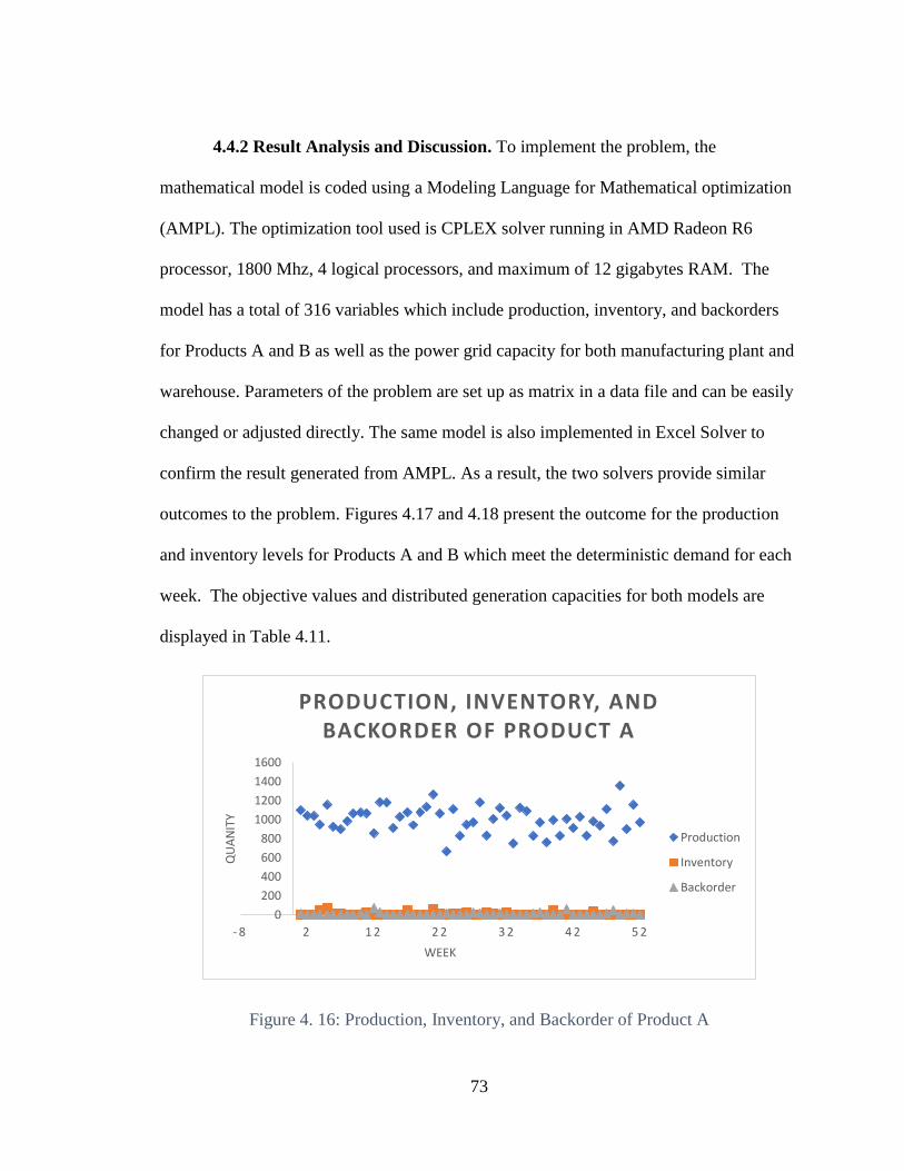
73
4.4.2 Result Analysis and Discussion. To implement the problem, the
mathematical model is coded using a Modeling Language for Mathematical optimization
(AMPL). The optimization tool used is CPLEX solver running in AMD Radeon R6
processor, 1800 Mhz, 4 logical processors, and maximum of 12 gigabytes RAM. The
model has a total of 316 variables which include production, inventory, and backorders
for Products A and B as well as the power grid capacity for both manufacturing plant and
warehouse. Parameters of the problem are set up as matrix in a data file and can be easily
changed or adjusted directly. The same model is also implemented in Excel Solver to
confirm the result generated from AMPL. As a result, the two solvers provide similar
outcomes to the problem. Figures 4.17 and 4.18 present the outcome for the production
and inventory levels for Products A and B which meet the deterministic demand for each
week. The objective values and distributed generation capacities for both models are
displayed in Table 4.11.
Figure 4. 16: Production, Inventory, and Backorder of Product A
0
200
400
600
800
1000
1200
1400
1600
- 8 2 1 2 2 2 3 2 4 2 5 2
QU
AN
ITY
WEEK
PRODUCTION, INVENTORY, AND BACKORDER OF PRODUCT A
Production
Inventory
Backorder
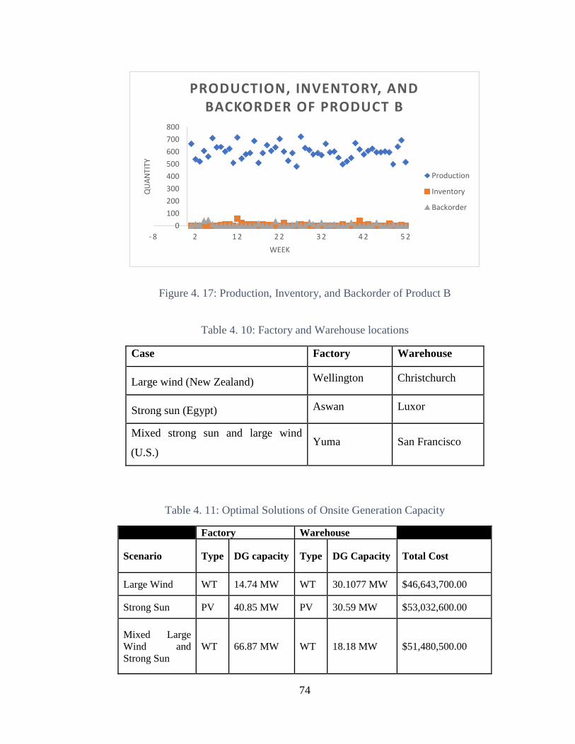
74
Figure 4. 17: Production, Inventory, and Backorder of Product B
Table 4. 10: Factory and Warehouse locations
Case Factory Warehouse
Large wind (New Zealand) Wellington Christchurch
Strong sun (Egypt) Aswan Luxor
Mixed strong sun and large wind
(U.S.) Yuma San Francisco
Table 4. 11: Optimal Solutions of Onsite Generation Capacity
Factory Warehouse
Scenario Type DG capacity Type DG Capacity Total Cost
Large Wind WT 14.74 MW WT 30.1077 MW $46,643,700.00
Strong Sun PV 40.85 MW PV 30.59 MW $53,032,600.00
Mixed Large
Wind and
Strong Sun
WT 66.87 MW WT 18.18 MW $51,480,500.00
0
100
200
300
400
500
600
700
800
- 8 2 1 2 2 2 3 2 4 2 5 2
QU
AN
TITY
WEEK
PRODUCTION, INVENTORY, AND BACKORDER OF PRODUCT B
Production
Inventory
Backorder

75
In the large wind case (Wellington and Christchurch) which has the highest levels
of WT capacity factors, we solve the mathematical model and the optimal cost is
$46,643,700.00. Given the carbon credit of $35/MWh for PV, the model chooses WT due
to the large wind condition in Wellington and Christchurch. Hence the resulting
aggregate installed capacity of WT in the factory is 14.74 MW and 30.11 MW for the
warehouse location.
The climate conditions in the strong sun location has low wind speed in both the
factory and warehouse sites. Even though WT installation cost is much lower than PV,
the model still chooses PV due to the given strong solar irradiance of Aswan and Luxor.
The installed capacity of PV in factory is 40.85 MW and at the warehouse is 30.59 MW.
The total annualized cost of the strong sun case is $53,032,600.
In the last case, mixed large wind and strong sun, the factory is located in Yuma,
Arizona with high solar irradiance, and the warehouse is in San Francisco with large
wind speed. In this mixed case, the model chooses WT for both the factory and
warehouse system. The outcome can be explained as follows. Even though Yuma has
strong sun, the model still chooses WT due to the low cost of WT system and the large
number of operation hours for the WT as it can generate power in 24/7. The resulting
aggregate installed capacity of WT in the factory is 66.87 MW and the capacity of WT in
the warehouse is 18.18 MW.
4.5 Conclusion
The study presented in this chapter was conducted at a practical level to represent
the operational conditions of real zero-carbon supply chains as much as possible. Wind
turbine (WT) and photovoltaic (PV) are alternative clean power sources which replace

76
traditional energy sources. Real data is collected in different cities, and a linear multi-
period production inventory model is used to find the minimum total cost (objective
function value) and the wind turbine (WT) capacity, photovoltaic (PV) capacity,
production, inventory, and backorders in each period (decision variables). This chapter
focused on chasing the most economic efficient way to replace traditional energy with
renewable energy to meet the factory and warehouse demands. The results from various
scenarios with data from different cities show that wind and PV generation is a proven
technology for manufacturing factories and warehousing activities to meet the electricity
consumption needs. As a result, the facilities can avoid borrowing electricity from main
grid when there is no wind or solar power available. In the next chapter, the model will
be extended to stochastic product demand under a multi-factory and single-warehouse
environment.

77
V. INTEGRATING MICROGRID POWER FOR NET-ZERO ENERGY
PRODUCTION-LOGISTICS WITH DEMAND UNCERTAINTY
5.1 Model Setting
In this chapter, the model setting is similar to Chapter 4 as e-trucks will be
employed to ship finished goods from factories to warehouse. The facilities and e-trucks
will be powered by the onsite microgrid system. Each microgrid system is comprised of
several WT units and (or) solar PV arrays. It is assumed that the distance between two
adjacent facilities is large enough so that wind profiles and weather conditions are not
correlated. In this chapter, we will also consider the adoption of a charging station on the
route between factories and warehouse. Assume the e-truck will charge its battery before
departing the facilities. If the maximum driving range is smaller than the distance
between two facilities, charging stations are available on route to recharge the vehicle
batteries. With this setting in mind, we aim at designing a net-zero carbon zone across
manufacturing, transportation, and warehousing facilities at minimum cost.
Figure 5. 1: Multi-Factory and One Distribution Center with Microgrid Generation

78
Since the daily wind speed and the weather conditions are stochastic, the output
power of the microgrid system at a random point in time may be above or below the
facility’s electricity load. If the output power is less than the load, the gap is fulfilled by
importing the electricity from the main grid. In order to attain net-zero energy criteria,
this “borrowed” electricity must be “returned” later on. This can be realized, for instance,
when large wind speed or strong sunshine prevails in certain days, making the microgrid
system to produce surplus energy. Feed-in-tariff and net-metering are the two market
schemes that enable the surplus electricity to be fed into the main grid. The production-
logistics system achieves the net-zero energy performance if the “borrowed” electricity is
offset by the surplus microgrid energy during the course of a year. Before presenting the
optimization model, the related notation is summarized in Table 5.1 below.
Table 5. 1: Model Parameters and Decision Variables
Notation Description
I =Total number of products
J =Total number of production periods
K =Total number of facilities where k=0 for the warehouse
G =number of renewable generation sources, for g=1, 2, .., G
R =number of resources required for producing the products, for r=1, 2, .., R
pijk =cost of making a unit of product i in period j in facility k ($/unit)
hij =unit holding cost of product i in period j ($/unit-period)
bij =unit backorder cost of product i in period j ($/unit)
ik =cost of shipping a unit of product i from facility k to the warehouse ($/unit)
viks =resource s consumed for making a unit of product i in facility k
wsjk =available resource of s in period j in facility k
qv =electric transport energy intensity rate (MWh/kg/km)
wp =the payload per trip between factory and warehouse (kg)

79
wv =vehicle self-weight (kg)
dk =distance between factory k and the warehouse (km)
Dij =demand for product i in period j
ijD =mean demand for product i in period j
ijD =standard deviation of demand for product i in period j
n =number of yearly trips between factory and warehouse
tw =annual operating hours of the warehouse (hours)
g =number of hours of generation g (hours) in each production period
ag =capacity cost for renewable generation g ($/MW)
bg =operation and maintenance cost for renewable generation g ($/MWh)
cg =carbon credits for renewable generation g ($/MWh)
jgk =capacity factor of renewable generator g in period j at location k
eik =energy consumed for producing one unit of product i (MWh/unit)
L =electricity demand (load) of the warehouse (MW)
=probability that the product demand is met
=capital recovery factor
wv =self-weight of the e-truck
=random wind profile and solar incidence on PV
Decision
Variable
Description
xijk =quantity of product i made in period j in facility k
yij =inventory of product i in period j in the warehouse
zij =backorder of product i in period j
Pcgk =capacity of generation source g in facility k
5.2 A Stochastic Optimization Model
We design a production-logistics system comprised of multiple factories and one
central warehouse which are powered entirely by onsite WT and PV systems. Each

80
factory will manufacture two types of product A and B. The finished goods from both
factories will then be shipped to the warehouse using e-truck. The objective of this study
is to determine the production quantity, inventory level, and backorders such that the
uncertain demands (stochastic demands) in each period are satisfied. Demand uncertainty
reflects uncertainty of customer demand for a product and it does not have stability. To
achieve the net zero energy target, the generation capacity of onsite microgrid systems is
also optimized so that the cost of the entire production-logistics system including energy
is minimized. Denote as Problem P2, the stochastic planning model formulated as follows
Problem P2:
Minimize:
( )
= = == =
=
−
== == = =
−++
+++=
G
g
K
k
J
j
gkgkggkgkg
G
g
K
k
c
gkg
I
i
J
j
ijij
I
i
J
j
ijij
I
i
J
j
K
k
ijkijkijk
c
PcPbEPa
zbyhxpf
1 0 11 0
1
1
11 11 1 1
)()(
)()P,z,y,x(
(5.1)
Subject to:
−
+−+=
1Pr 11,1,0,
1
1, iikikik
K
k
ik Dzyyx ; for j=1, and i (5.2)
−
+−−+ −−
=
1Pr ,1,1
1
ijijkkijijkkij
K
k
ijk Dzzyyx ; for j=2, 3, .., J-1, and i
(5.3)
−
−−+ −−
=
1Pr ,1,1
1
iJkiJiJkkiJ
K
k
iJk Dzyyx ; for j=J, and i (5.4)
jkrijk
I
iikr wxv
=1
, for j, r, and k =1, 2.., K (5.5)
= == =
=++J
j
G
g
gkgk
v
kkv
I
i
J
j
ijkikvik PEwdnqxmdqe1 11 1
)()( , for k=1, 2 …, K.
(5.6)
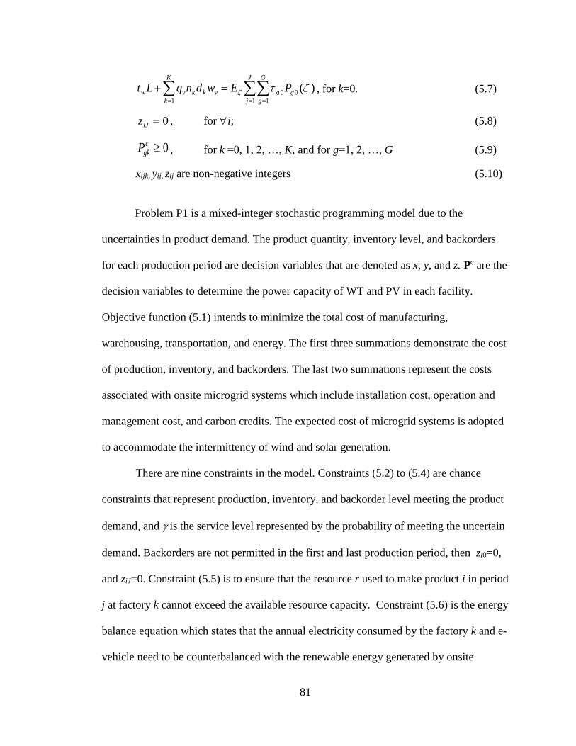
81
= ==
=+J
j
G
g
gg
K
k
vkkvw PEwdnqLt1 1
00
1
)( , for k=0. (5.7)
0=iJz , for i; (5.8)
0c
gkP , for k =0, 1, 2, …, K, and for g=1, 2, …, G (5.9)
xijk, yij, zij are non-negative integers (5.10)
Problem P1 is a mixed-integer stochastic programming model due to the
uncertainties in product demand. The product quantity, inventory level, and backorders
for each production period are decision variables that are denoted as x, y, and z. Pc are the
decision variables to determine the power capacity of WT and PV in each facility.
Objective function (5.1) intends to minimize the total cost of manufacturing,
warehousing, transportation, and energy. The first three summations demonstrate the cost
of production, inventory, and backorders. The last two summations represent the costs
associated with onsite microgrid systems which include installation cost, operation and
management cost, and carbon credits. The expected cost of microgrid systems is adopted
to accommodate the intermittency of wind and solar generation.
There are nine constraints in the model. Constraints (5.2) to (5.4) are chance
constraints that represent production, inventory, and backorder level meeting the product
demand, and is the service level represented by the probability of meeting the uncertain
demand. Backorders are not permitted in the first and last production period, then zi0=0,
and ziJ=0. Constraint (5.5) is to ensure that the resource r used to make product i in period
j at factory k cannot exceed the available resource capacity. Constraint (5.6) is the energy
balance equation which states that the annual electricity consumed by the factory k and e-
vehicle need to be counterbalanced with the renewable energy generated by onsite
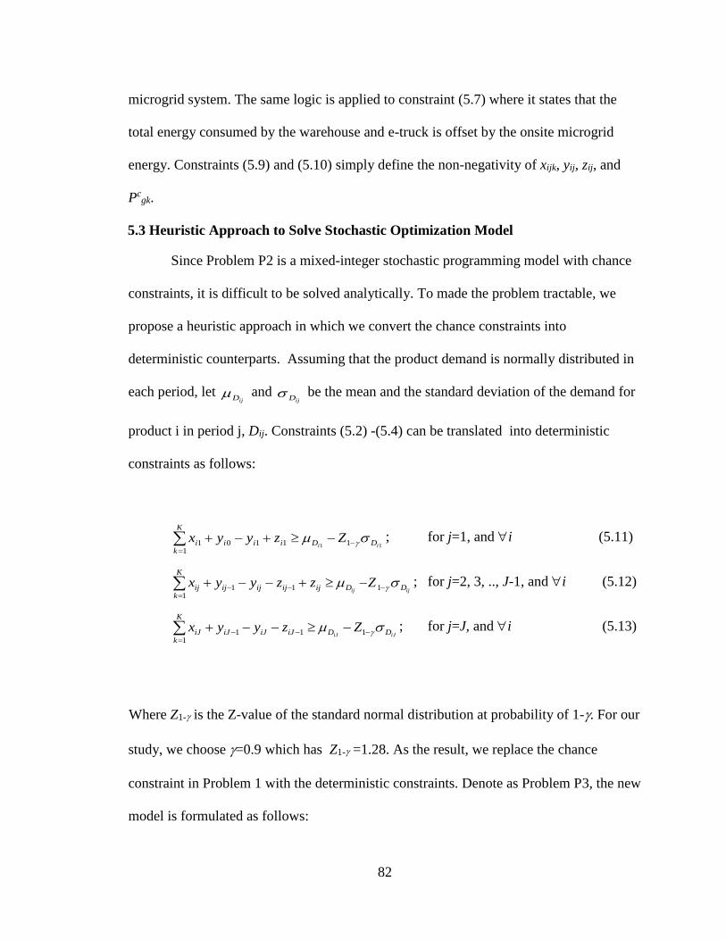
82
microgrid system. The same logic is applied to constraint (5.7) where it states that the
total energy consumed by the warehouse and e-truck is offset by the onsite microgrid
energy. Constraints (5.9) and (5.10) simply define the non-negativity of xijk, yij, zij, and
Pcgk.
5.3 Heuristic Approach to Solve Stochastic Optimization Model
Since Problem P2 is a mixed-integer stochastic programming model with chance
constraints, it is difficult to be solved analytically. To made the problem tractable, we
propose a heuristic approach in which we convert the chance constraints into
deterministic counterparts. Assuming that the product demand is normally distributed in
each period, let ijD and
ijD be the mean and the standard deviation of the demand for
product i in period j, Dij. Constraints (5.2) -(5.4) can be translated into deterministic
constraints as follows:
11 11101
1 ii DDiii
K
ki Zzyyx −
=
−+−+ ; for j=1, and i (5.11)
ijij DDijijijij
K
kij Zzzyyx −−−
=
−+−−+ 1111
; for j=2, 3, .., J-1, and i (5.12)
iJiJ DDiJiJiJ
K
kiJ Zzyyx −−−
=
−−−+ 1111
; for j=J, and i (5.13)
Where Z1- is the Z-value of the standard normal distribution at probability of 1-. For our
study, we choose =0.9 which has Z1- =1.28. As the result, we replace the chance
constraint in Problem 1 with the deterministic constraints. Denote as Problem P3, the new
model is formulated as follows:
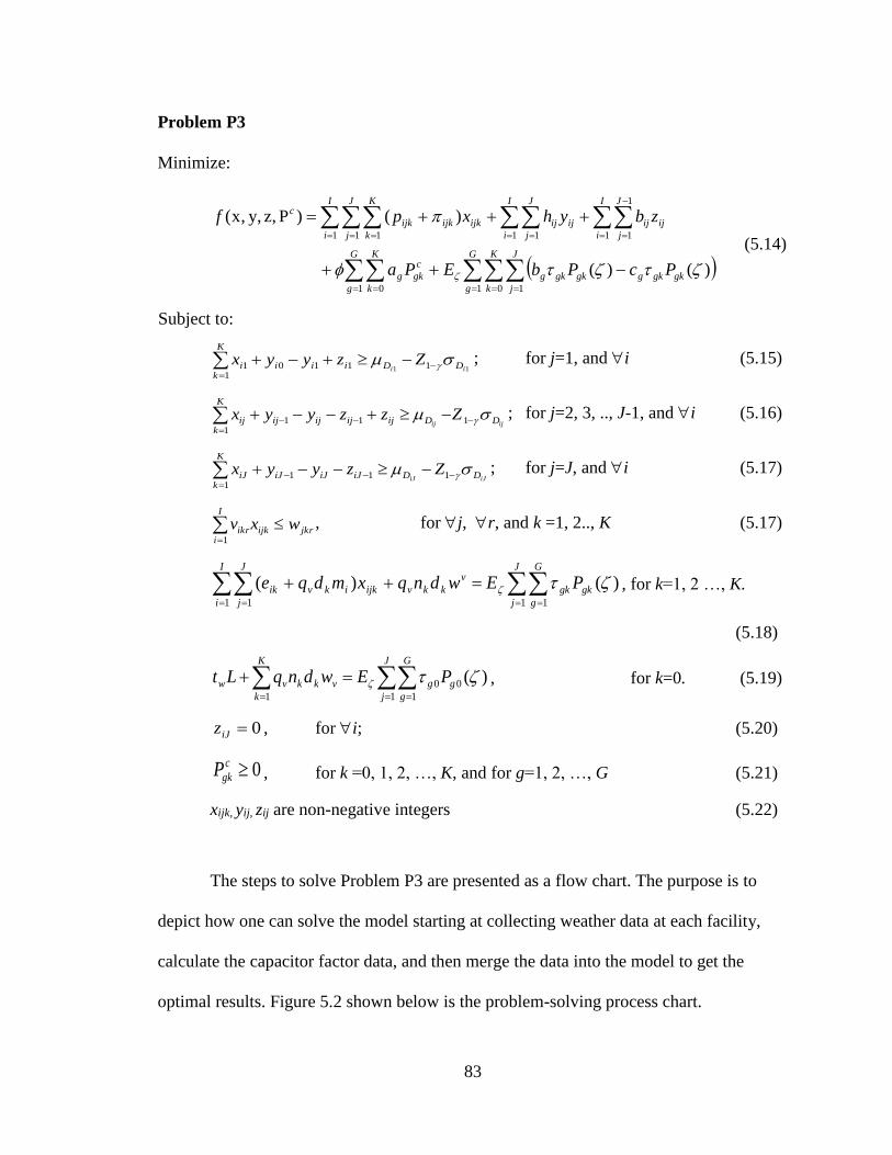
83
Problem P3
Minimize:
( )
= = == =
=
−
== == = =
−++
+++=
G
g
K
k
J
j
gkgkggkgkg
G
g
K
k
c
gkg
I
i
J
j
ijij
I
i
J
j
ijij
I
i
J
j
K
k
ijkijkijk
c
PcPbEPa
zbyhxpf
1 0 11 0
1
1
11 11 1 1
)()(
)()P,z,y,x(
(5.14)
Subject to:
11 11101
1 ii DDiii
K
ki Zzyyx −
=
−+−+ ; for j=1, and i (5.15)
ijij DDijijijij
K
kij Zzzyyx −−−
=
−+−−+ 1111
; for j=2, 3, .., J-1, and i (5.16)
iJiJ DDiJiJiJ
K
kiJ Zzyyx −−−
=
−−−+ 1111
; for j=J, and i (5.17)
jkrijk
I
iikr wxv
=1
, for j, r, and k =1, 2.., K (5.17)
= == =
=++J
j
G
g
gkgk
v
kkv
I
i
J
j
ijkikvik PEwdnqxmdqe1 11 1
)()( , for k=1, 2 …, K.
(5.18)
= ==
=+J
j
G
g
gg
K
k
vkkvw PEwdnqLt1 1
00
1
)( , for k=0. (5.19)
0=iJz , for i; (5.20)
0c
gkP , for k =0, 1, 2, …, K, and for g=1, 2, …, G (5.21)
xijk, yij, zij are non-negative integers (5.22)
The steps to solve Problem P3 are presented as a flow chart. The purpose is to
depict how one can solve the model starting at collecting weather data at each facility,
calculate the capacitor factor data, and then merge the data into the model to get the
optimal results. Figure 5.2 shown below is the problem-solving process chart.

84
Figure 5. 2: Process Chart to Solve the Model (Pham et al. 2017)
5.4 Numerical Experiment for Single Factory – Single Warehouse Model
5.4.1 Problem setting and data. We first implement P3 on a single factory and a
single warehouse setting. Similar to Chapter 4, the production data used for this
experiment are also associated with the wafer production facilities that operate in 24/7
mode. Two types of products are manufactured at the factory which are Product A and
Product B. The product demands for each week are uncertain but follow a normal
distribution. The mean demand for Product A per week is 1,000 units with the standard
deviation of 120 units. The mean demand for Product B per week is 600 units with
Collect climatic data from Unground Weather
Webpage portal for a particular location
Daily ground wind
speed
in a particular location
Daily sunshine pattern
in a particular location
extrapolate solar
irradiance distribution
for a production
period (e.g. one week)
Estimate the mean and
variance of wind speed
at WT tower height
Extrapolate wind speed
distribution for a
production period
• Estimate the capacity factor for WT system
• Estimate the capacity factor for PV system
Solve Problem P4-2
Find optimal Pc
Min: f2(Pc; x, y, z)
Solve Problem P4-1
Find optimal {x, y, x}
Min: f1(x, y, z)
Forecasting the product
demands, and estimating the
mean and variance for each
period
Transform the Chance
constraints into deterministic
constraints based on normality
Renewable Generation Analytics Two-Stage Optimization
Estimate the
maximum solar
irradiance sm
Net-Zero Energy Production-Logistics
Modeling and Planning
Solve Problem P3
Find optimal Pc
Min: f (Pc, x, y, z)
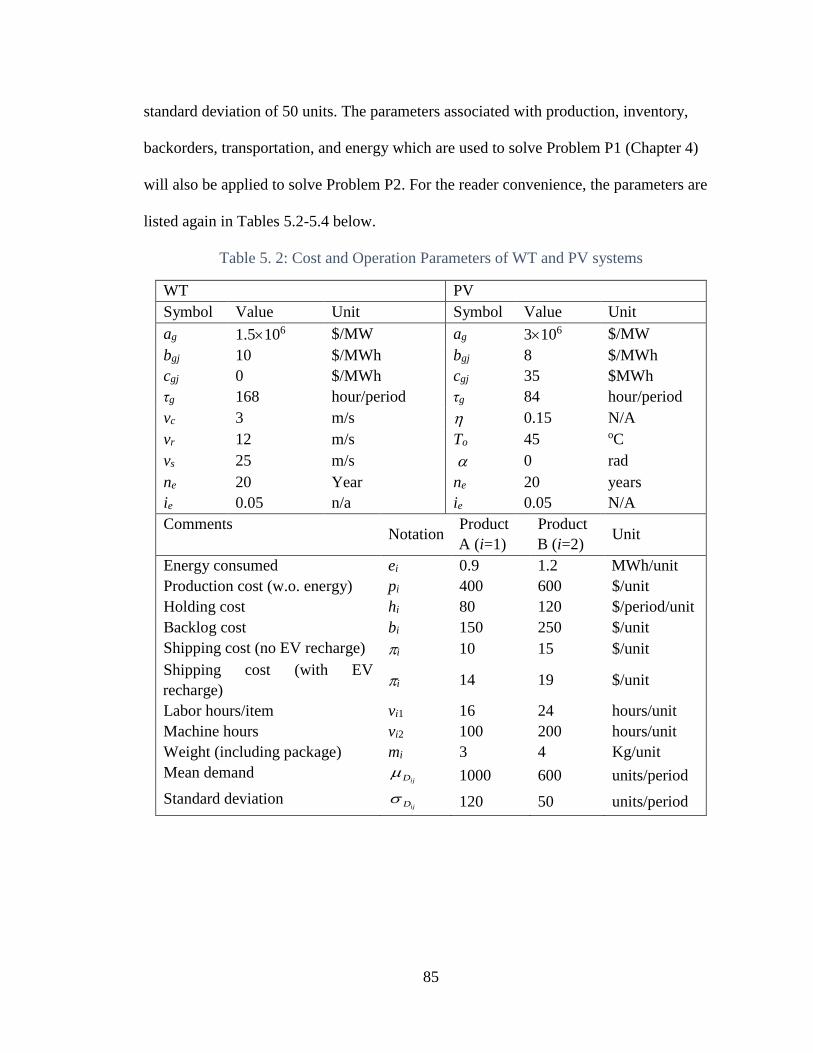
85
standard deviation of 50 units. The parameters associated with production, inventory,
backorders, transportation, and energy which are used to solve Problem P1 (Chapter 4)
will also be applied to solve Problem P2. For the reader convenience, the parameters are
listed again in Tables 5.2-5.4 below.
Table 5. 2: Cost and Operation Parameters of WT and PV systems
WT PV
Symbol Value Unit Symbol Value Unit
ag 1.5106 $/MW ag 3106 $/MW
bgj 10 $/MWh bgj 8 $/MWh
cgj 0 $/MWh cgj 35 $MWh
τg 168 hour/period τg 84 hour/period
vc 3 m/s 0.15 N/A
vr 12 m/s To 45 oC
vs 25 m/s 0 rad
ne 20 Year ne 20 years
ie 0.05 n/a ie 0.05 N/A
Comments Notation
Product
A (i=1)
Product
B (i=2) Unit
Energy consumed ei 0.9 1.2 MWh/unit
Production cost (w.o. energy) pi 400 600 $/unit
Holding cost hi 80 120 $/period/unit
Backlog cost bi 150 250 $/unit
Shipping cost (no EV recharge) i 10 15 $/unit
Shipping cost (with EV
recharge) i 14 19 $/unit
Labor hours/item vi1 16 24 hours/unit
Machine hours vi2 100 200 hours/unit
Weight (including package) mi 3 4 Kg/unit
Mean demand 1000 600 units/period
Standard deviation 120 50 units/period
ijD
ijD

86
Table 5. 3: Machine and Labor Resources in the Factory
Week
Labor
Resource
(hours)
Machine or
Tool Resource
(hours)
Week
Labor
Resource
(hours)
Machine or Tool
Resource (hours)
1 38,516 278,847 27 37,860 279,542
2 34,429 244,299 28 39,153 281,016
3 33,472 239,044 29 32,345 237,514
4 34,210 248,699 30 34,562 249,292
5 36,680 261,478 31 36,814 263,851
6 36,660 269,935 32 35,001 251,627
7 34,063 249,447 33 32,159 239,152
8 35,786 261,961 34 37,138 269,049
9 36,243 261,441 35 36,784 267,032
10 36,989 268,359 36 30,487 223,362
11 33,739 240,138 37 31,639 226,421
12 35,560 263,343 38 28,497 208,141
13 36,920 262,138 39 33,601 241,714
14 37,695 268,946 40 33,727 249,509
15 33,051 240,437 41 35,735 259,884
16 38,113 276,789 42 32,750 237,912
17 33,914 241,252 43 35,657 257,745
18 33,569 243,591 44 32,635 240,033
19 38,010 274,606 45 34,452 249,525
20 37,688 270,170 46 33,684 244,778
21 40,853 291,900 47 37,094 267,545
22 38,946 283,740 48 30,751 226,419
23 28,867 215,059 49 38,739 270,781
24 34,891 248,255 50 34,252 250,829
25 31,466 230,446 51 40,363 292,169
26 30,652 219,114 52 32,078 230,129

87
Table 5. 4: Cost and Operation Parameters of WT and PV systems
WT PV
Symbol Value Unit Symbol Value Unit
ag 1.5106 $/MW ag 3106 $/MW
bgj 10 $/MWh bgj 8 $/MWh
cgj 0 $/MWh cgj 35 $MWh
τg 168 hour/period τg 84 hour/period
vc 3 m/s 0.15 N/A
vr 12 m/s To 45 oC
vs 25 m/s 0 rad
ne 20 Year ne 20 years
ie 0.05 n/a ie 0.05 N/A
As mentioned in the problem station, transportation cost is added in this model to
accurately estimate the cost of operation. To estimate the transportation cost, two
scenarios are considered with dmax=150 km.
• Scenario 1: If an e-truck can travel from the factory to the warehouse without
recharging the battery (i.e. dk<dmax) on route, then 1 = $10 per unit and 2 =
$15 per unit.
• Scenario 2: If an e-truck requires the battery recharging because of dk>dmax,
then 1 = $14 per unit and 2 = $19 per unit. These larger costs vs. the ones in
scenario one are to include bills for recharging the vehicles and the e-truck
waiting time.
5.4.2 Result analysis and discussion. To test the model in different cities,
Problem P3 is coded using a Modeling Language for Mathematical Programing (AMPL)
software using the CPLEX solver running in the AMD Radeon R6 processor, which runs
at 1.8 GHz and contains 4 cores, and 12 GB DRAM. The current model has a total of 316
decision variables including production quantity, inventory, and backorders, and the
capacity of onsite WT and PV of each facility. Parameters of the problem are arranged as

88
a matrix in a data file and can be easily changed or adjusted to solve the problem varying
the values for the parameters. Figures 5.3 and 5.4 present the resulting production,
inventory, and backorders for Products A and B across 52 weeks. The model is solved
with =0.9 to meet the product demands.
Figure 5. 3: Decision on Product A for Model P2-1
Figure 5. 4: Decision on Product B for Model P2-1
0
200
400
600
800
1000
1200
1400
1600
0 10 20 30 40 50
Qu
anti
ty
Week
Production, Inventory and backorders for Product A
Production
Inventory
Backorders
0
100
200
300
400
500
600
700
800
900
0 10 20 30 40 50
Qu
anti
ty
Week
Production, Inventory and backorders for Product B
Production
Inventory
Backorders

89
Table 5. 5: Results of Three Different Production-Logistics Systems
Case 1 2 3
City Wellington Aswan Yuma
Facility Factory Factory Factory
Wind profile Strong wind Low wind Medium wind
Weather condition Weak sun Strong sun Strong sun
Generation type WT PV WT
Capacity (MW) 16.59 46.09 75.34
City Christchurch Luxor San Francisco
Facility Warehouse Warehouse Warehouse
Wind profile Strong wind Low wind Medium wind
Weather condition Weak sun Strong sun Medium sun
Generation type WT PV WT
Capacity (MW) 30.08 30.55 18.18
Travel distance (km) 439 238 1051
Annualized system cost $54,229,900 $61,257,100 $59,869,200
Case 1 represents the strong wind scenarios in the factory and the warehouse. For
Case 1, the model chooses WT generation type for both the factory and warehouse. Given
the carbon credit of $35/MWh for PV system, the model chooses WT system due to the
significant strong wind condition in both locations. The minimum total cost is
$54,229,900 which covers production-inventory cost, energy, and transportation cost.
The installed capacity for the factory is 16.5 MW while for the warehouse is 30.08 MW.
In Case 2, we consider the city of Aswan and Luxor with strong sun condition and
low wind speed profile. Opposite to Case 1, in this experiment, the model chooses to
install PV generation system for both the factory and the warehouse despite the
installation and maintenance cost for PV system is twice of the WT system. It is
predictable since both cities have strong sunshine throughout the year. The capacity
required for onsite PV generation is 46.12 MW for the factory and 30.57 MW for the
warehouse. The annual minimum operational cost is $61,265,100.

90
In Case 3, we study a mixed weather scenario in which the factory is located in Yuma,
AZ which has strong sun profile with medium wind speed, and the warehouse is located
in San Francisco, CA with medium wind speed and medium sunshine. In this experiment,
the model chooses WT for both the factory and the warehouse as optimal solutions. Even
though Yuma is known for its strong sun, the model still chooses wind generation despite
the PV carbon credit of $35/MWh. The installed WT capacity in the factory is 75.34 MW
and the WT capacity in the warehouse is 18.18 MW. The annualized system cost is
$59,869,200.
5.5 Multi-Factory Production and Logistics Systems
5.5.1 System setting and parameters. In this experiment, we will solve Problem
P3 under a two-factory and one-warehouse setting. The two factories will be located at
Yuma, Arizona and El Paso, Texas, and Phoenix, Arizona is chosen for the warehouse
site. The average weather conditions of the cities can be observed in Table 5.6 and the
average wind speeds for all the cities are shown in Figure 5.5.
Table 5. 6: Average weather condition of 4 cities
Country USA
City Yuma San
Francisco El Paso Phoenix
Latitude (Deg) 32.69 37.77 31.76 33.45
Ground AWS 2.97 4.05 2.8 3.76
Ground SWS 1.4 1.83 1.05 1.78
Clear days 165 28 61 66
Scattered Cloud 109 95 111 115
Partially Cloudy 65 136 108 133
Mostly Cloudy 0 13 5 4
Overcast 0 2 1 1
Rain 13 65 31 25
Fog 1 24 2 0
Storm/T-Storms 11 3 41 22
Snow 0 0 5 0

91
Figure 5. 5: The Weekly Solar PV Capacity Factor of Eight Cities
Two factories located in Yuma and San Francisco are capable of manufacturing
two types of products, namely A and B. All the finished goods will be shipped to the
warehouse located at Phoenix via e-truck. Assume the frequency between the factories
and the warehouse is nk = 186 trips/year. All the parameters and setting for this
experiment will be the same as Section 5.4. The available labor and machine hours for
each factory are listed in Table 5.7.
0.0
0.1
0.2
0.3
0.4
0.5
0.6
0 5 10 15 20 25 30 35 40 45 50
PV
Cap
acit
y F
acto
r
Week
Wellington Christchurch Aswan Luxor
Yuma San Francisco El Paso Phonix

92
Table 5. 7: Production demand for two factories
(Factory 1=Yuma, Factory 2=El Paso)
Week Labor Hours Machine Hours
Week Labor Hours Machine Hours
Factory
1
Factory
2
Factory
1
Factory
2
Factory
1
Factory
2
Factory
1
Factory
2
1 22,339 16,177 153,366 125,481 27 21,959 15,901 153,748 125,794
2 19,969 14,460 134,365 109,935 28 22,709 16,444 154,559 126,457
3 19,414 14,058 131,474 107,570 29 18,760 13,585 130,633 106,881
4 19,842 14,368 136,784 111,915 30 20,046 14,516 137,111 112,182
5 21,275 15,406 143,813 117,665 31 21,352 15,462 145,118 118,733
6 21,263 15,397 148,464 121,471 32 20,301 14,701 138,395 113,232
7 19,757 14,306 137,196 112,251 33 18,652 13,507 131,533 107,618
8 20,756 15,030 144,078 117,882 34 21,540 15,598 147,977 121,072
9 21,021 15,222 143,793 117,648 35 21,335 15,449 146,868 120,165
10 21,453 15,535 147,598 120,762 36 17,682 12,804 122,849 100,513
11 19,568 14,170 132,076 108,062 37 18,351 13,288 124,532 101,890
12 20,625 14,935 144,839 118,504 38 16,528 11,969 114,477 93,663
13 21,413 15,506 144,176 117,962 39 19,488 14,112 132,943 108,771
14 21,863 15,832 147,920 121,026 40 19,562 14,165 137,230 112,279
15 19,170 13,881 132,241 108,197 41 20,726 15,009 142,936 116,948
16 22,106 16,008 152,234 124,555 42 18,995 13,755 130,852 107,060
17 19,670 14,244 132,688 108,563 43 20,681 14,976 141,760 115,985
18 19,470 14,099 133,975 109,616 44 18,928 13,707 132,018 108,015
19 22,046 13,303 151,033 123,573 45 19,982 14,470 137,239 112,286
20 21,859 15,829 148,593 121,576 46 19,536 14,147 134,628 110,150
21 23,695 17,158 160,545 131,355 47 21,515 15,580 147,150 120,395
22 22,589 16,357 156,057 127,683 48 17,836 12,915 124,530 101,889
23 16,743 12,124 118,283 96,777 49 22,469 16,270 148,930 121,852
24 20,237 14,654 136,540 111,715 50 19,866 14,386 137,956 112,873
25 18,250 13,216 126,745 103,701 51 23,410 14,127 160,693 131,476
26 17,778 12,874 120,513 98,601 52 18,605 13,473 126,571 103,558
5.5.2 Results and discussion. The model outputs for the production-inventory
level that meet the stochastic demand weekly with 90% confidence level are
demonstrated in Figures 5.6 and 5.7. Figure 5.6 represents the production-inventory level
for Product A in both Factories 1 and 2 while Figure 5.7 displays the production-
inventory level for Product B in both factories. This model has total of 422 decision

93
variables which include production quantity of each factory, warehouse inventory, and
backorders as well as the onsite generation capacity of WT and PV in each facility.
Figure 5. 6: Results of Product A
Figure 5. 7: Results of Product A
0
200
400
600
800
1000
1200
0 10 20 30 40 50
Qu
anti
ty
Week
Multi-Facility Production Planning for Product A
Factory 1 (Yuma) Factory 2 (El Paso)
Inventory (Phoenix) Backorders
0
100
200
300
400
500
600
700
0 10 20 30 40 50
Quan
tity
Week
Multi-Facility Production Planning for Product B
Factory 1 (Yuma) Factory 2 (El Paso)
Inventory (Phoenix) Backorders

94
The results of the model are presented in three cases and summarized in Table
5.8. Case 4 is the baseline corresponding to the situation where the PV capacity cost is
$3M/MW and its carbon credit is $35/MWh. We solve Problem P3 and the annualized
system cost is $61,243,500. Despite the strong sunshine in Phoenix and the favorable
carbon credit of $35/MWh, the model chooses WT as the power generator. The same
results are observed in El Paso and Yuma where WT is more cost-effective than PV
regardless of strong sunshine in these sites.
Table 5. 8: Comparisons under Different PV Cost and Carbon Credits
Case 4 Case 5 Case 6
PV capacity Cost
($/MW) 3106 2106 1.5106
PC Carbon credit
($/MWh) 35 0 0
Type
Capacity
(MW) Type
Capacity
(MW) Type
Capacity
(MW)
Factory 1 (Yuma) WT 43.8 WT 43.8 PV 36.81
Factory 2 (El Paso) WT 18.56 WT 18.56 WT 18.56
Warehouse (Phoenix) WT 72.41 PV 52.95 PV 52.95
Annualized system cost $61,243,500 $60,903,800 $57,828,100
Cases 5 and 6 are designed for sensitivity analysis. In Case 5, the PV capacity
cost is reduced to $2M/MW with no carbon credit. The model chooses PV for Phoenix,
and WT for Yuma and El Paso with the cost of $60,908,800. This is slightly lower than
the cost in Case 4. In Case 6, the PV capacity cost goes down to $1.5M/MW which is the
same as the WT cost. The model shows that El Paso still chooses WT, but in Yuma PV
becomes more cost-effective than WT. The annualized cost is $57,828,100, which is
5.6% lower than Case4.

95
Finally, we compute the levelized energy cost (LEC) of each location, and
determine which site is cost-effective for large-scale microgrid generation. LEC is the net
present value of the unit-cost of electricity over the lifetime of a generating asset. Based
on the results in Table 5.9, using $70/MWh as the reference utility price, Wellington,
Christchurch, San Francisco and El Paso are cost-effective in harnessing onsite wind
generation. Phoenix is a city favorable for PV generation, but at the $3M/MW capacity
cost, its LEC is more than twice of current utility price. If we project the utility price in
20 years, the rate will reach $120/MWh under 3% annual increase. This means all the
eight cities except Phoenix are favorable to install WT, PV or both over the 20-year
horizon.
Table 5. 9: Levelized Cost of Renewable Energy
(H=high, M=medium, L=Low)
City
Annual Non-
Energy Cost
($)
Annual
Energy Cost
($)
Annual
Electricity
Use (MWh) $/MWh
Cost
Effective
Wellington 46,207,500 2,950,330 95,509 31 H
Christchurch 840,685 4,231,300 61,216 69 H
Aswan 46,207,500 8,513,820 95,509 89 M
Luxor 840,685 5,695,030 61,216 93 M
Yuma 46,207,500 10,019,800 95,509 105 M
San
Francisco 840,685 2,801,190
61,216 46
H
Yuma 25,008,900 5,824,760 55,562 105 M
El Paso 17,611,900 2,633,280 39,987 66 H
Phoenix 839,714 9,324,970 61,262 152 L
96
VI. NET ZERO CARBON SUPPLY CHAIN NETWORK UNDER
DETERMINISTIC AND STOCHASTIC DEMAND
6.1 Supply Chain with Microgrid Power and Deterministic Demand
6.1.1 Model setting. Figure 1 describes a supply chain comprised of multiple
manufacturers, warehouses, and stores, and e-trucks that are used to transport product
between different locations. Assume all the factories are capable of manufacture Products
A and B. Similar to the previous chapters, the energy needed to operate the entire supply
chain is provided by the onsite microgrid generations. Each microgrid will consider two
type of renewable energy which are wind turbine (WT) and photovoltaic (PV). The e-
vehicle fleet also use the onsite generated energy to charge their battery. If the driving
distance between two facilities is greater than the driving range of e-vehicle battery,
charging stations will be created within the route so the e-vehicles can recharge their
battery. With the use of onsite renewable energy generation for production and
transportation, our goal is to create a supply chain network with net zero carbon
emissions.
Net-metering will be considered also in the case of energy surplus or shortage. If
the energy output cannot meet the load demand of the facilities, conventional energy can
be borrowed to power the facilities. This amount of “borrowed” energy will be paid back
during a period when the energy generated by the onsite generation system exceeds the
amount required by the local facilities.

97
Figure 6. 1: Supply Chain with Microgrid Generation
6.1.2 Optimization Algorithm.
a. Mathematical model notations.
Notation Explanations
I number of product types
J number of production periods
M number of factories
K number of warehouses
S number of retail stores
G number of renewable generation sources
R number of resources required for production

98
pim cost of making a unit of product i at factory m ($/unit)
hik unit holding cost of product i at warehouse k ($/period)
bi unit backorder cost of product i ($/unit)
i cost of shipping a unit of product i ($/unit)
viml resource l consumed for making a unit of product i in factory m
wljm available resource of l in period j in factory m
qv electric transport energy intensity rate (MWh/kg/km)
mi the weight of product i (kg)
wv vehicle self-weight (kg)
dm distance between factory m and the warehouse (km)
ds distance between retail store s and the warehouse (km)
Dijs demand for product i in period j for retail store s
ijD mean demand for product i in period j
ijD standard deviation of demand for product i in period j
nmk number of yearly trips between factory m and warehouse k
njks number of yearly trips between warehouse k and retail store s
tw annual operating hours of the warehouse (hours)
ts annual operating hours of retail stores (hours)
g number of hours of generation g (hours) in each production period
ag capacity cost for renewable generation g ($/MW)
bg operation and maintenance cost for renewable generation g ($/MWh)
cg carbon credits for renewable generation g ($/MWh)
jgm capacity factor of renewable generator g in period j at factory m
jgk capacity factor of renewable generator g in period j at warehouse k
jgs capacity factor of renewable generator g in period j at retail store s
eim energy consumed for producing one unit of product i at factory m (MWh/unit)
Lw electricity demand (load) of the warehouse (MW)
Ls electricity demand (load) of the retail store (MW)
probability that the product demand is met
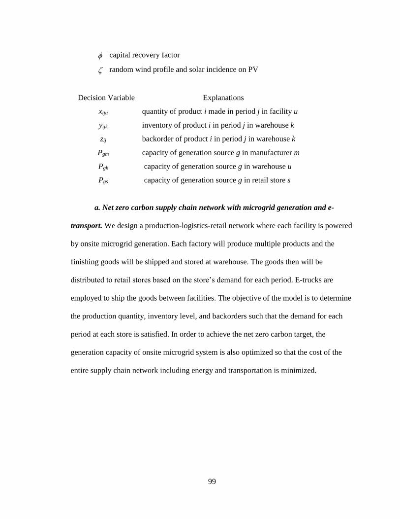
99
capital recovery factor
random wind profile and solar incidence on PV
Decision Variable Explanations
xiju quantity of product i made in period j in facility u
yijk inventory of product i in period j in warehouse k
zij backorder of product i in period j in warehouse k
Pgm capacity of generation source g in manufacturer m
Pgk capacity of generation source g in warehouse u
Pgs capacity of generation source g in retail store s
a. Net zero carbon supply chain network with microgrid generation and e-
transport. We design a production-logistics-retail network where each facility is powered
by onsite microgrid generation. Each factory will produce multiple products and the
finishing goods will be shipped and stored at warehouse. The goods then will be
distributed to retail stores based on the store’s demand for each period. E-trucks are
employed to ship the goods between facilities. The objective of the model is to determine
the production quantity, inventory level, and backorders such that the demand for each
period at each store is satisfied. In order to achieve the net zero carbon target, the
generation capacity of onsite microgrid system is also optimized so that the cost of the
entire supply chain network including energy and transportation is minimized.

100
Problem P4:
Minimize:
=
−
==
−
= == = =
+++=I
i
J
j
iji
I
i
J
j
K
k
ijkik
I
i
J
j
M
m
ijmiijm
c zbyhxpf1
1
11
1
1 11 1 1
)()P,z,y,x(
= = = =
+++G
g
M
m
K
k
S
s
c
gs
c
gk
c
gmg PPPa1 1 1 1
)(
( )= = = = =
++−+G
g
K
k
J
j
M
m
S
s
c
gsgjs
c
gkgjk
c
gmgjmggg PPPcb1 0 1 1 1
)(
(6.1)
Subject to:
ijs
S
s
ijkijk
M
m
K
k
ijm Dzyx == =
+−11 1
)( , j= 1 and i, k, u, s (6.2)
=
−−
= =
−+−+S
s
ijskjiijkijkkji
M
m
K
k
ijm Dzzyyx1
,1,,1,
1 1
)( ,
for j= 2,3,..,J-1 and i, k, u, s (6.3)
ljm
I
i
ijmilm wxv =1
, for i and j (6.4)
𝑧𝑖𝑘,𝐽 = 0 for i and k (6.5)
= == =
=++J
j
G
g
c
gmgjmg
v
mmkv
I
i
J
j
ijmimmkvim Pwdnqxmdnqe1 11 1
)( (6.6)
= == = ==
=+++J
j
G
g
c
gkgjkg
I
i
J
j
S
s
sjksv
v
ijsi
J
j
v
mmkvww PdnqwDmwdnqLt1 11 1 11
)( (6.7)
= ==
=+J
j
G
g
c
gsg
J
j
v
sjksvss PwdnqLt1 11
(6.8)
0,, c
gs
c
gk
c
gu PPP , for g, k, u, s (6.9)

101
xijm, yijk, zijk are non-negative integers (6.10)
Problem P4 is a mixed-integer linear programming model in which x, y, and z are
decision variables representing the production, inventory, and backorders in each period;
Pc is the decision variables for the power capacity of WT and PV in each facility.
Objective function (6.1) is to minimize the total cost comprised of manufacturing,
transportation, warehousing, and energy. The first three summations represent the
production (including shipping), inventory and backorder costs. The last two summations
capture the costs associated with microgrid installation, maintenance & operations, and
carbon credits. The expected cost of microgrid systems is adopted to accommodate the
intermittency of wind and solar generation.
Constraint (6.6) is the renewable energy balance equation, stating that the annual
electricity consumed by factory k and the forward logistics is fully offset by onsite
microgrid energy. qv is the electric vehicle energy intensity rate at speed v for which
calculation information can be found in chapter 3. Constraint (6.7) defines the energy
balance of the warehouse, stating that the total warehouse energy including the reverse
logistics to the factories and the forward logistics to retail stores is fully offset by the
onsite microgrid energy. njks is the number of weekly trips between warehouse k and
retail store s where 𝑛𝑗𝑘𝑠 = 𝐷𝑒𝑚𝑎𝑛𝑑 ×𝑝𝑟𝑜𝑑𝑢𝑐𝑡 𝑤𝑒𝑖𝑔ℎ𝑡
max 𝑤𝑒𝑖𝑔ℎ𝑡 𝑜𝑓 𝑔𝑜𝑜𝑑 𝑎𝑙𝑙𝑜𝑤 . Constraint (6.8) indicates that the
total energy used by the retail stores including the reverse logistics is fully offset by the
onsite microgrid energy. Constraints (6.9) and (6.10) simply define the non-negativity of
xijk, yij, zij, and Pc.

102
6.1.3 Renewable Generation Analytics.
a. Climate Data Collection. To demonstrate the feasibility of net-zero energy
supply chain operations, ten cities located in different regions of U.S. are selected to test
the model in P4. The latitude, average wind speed, and weather conditions of each city
are summarized in Table 6.1. Note that San Francisco, San Jose, Los Angeles,
Sacramento are in California, Tucson, Yuma, and Phoenix are in Arizona, Reno and Las
Vegas are in Nevada, and Salt Lake City is in Utah. The daily wind speed and the
weather patterns of these cities are retrieved from the Weather Underground web portal
(WeatherUnderground,2017). The weather conditions are classified into eight states,
namely, clear day, scattered cloud (SC), partially cloudy (PC), mostly cloudy (MC),
overcast, rain, fog, storm/T-storm and snow.
For each city, average wind speed and weather conditions over a range of eleven
years (from 2006 to 2016) are collected to accurately capture a long range of climate
conditions. There are 4,015 daily wind speed measurements collected for each city, and
these speed data will be used to estimate the WT capacity factors for ten cities. This also
applies for weather conditions where 4,015 data points are obtained from weather
underground website for the span of eleven years. There are total of 40,150 weather
conditions data collected between 2006 and 2016 for ten cities. The size of dataset for
this analytic method reaches 80,300 data points.
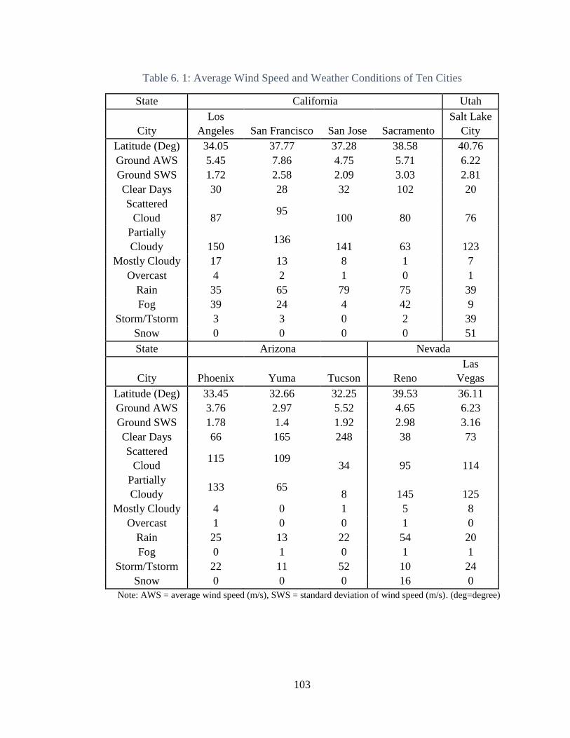
103
Table 6. 1: Average Wind Speed and Weather Conditions of Ten Cities
State California Utah
City
Los
Angeles San Francisco San Jose Sacramento
Salt Lake
City
Latitude (Deg) 34.05 37.77 37.28 38.58 40.76
Ground AWS 5.45 7.86 4.75 5.71 6.22
Ground SWS 1.72 2.58 2.09 3.03 2.81
Clear Days 30 28 32 102 20
Scattered
Cloud 87 95
100 80 76
Partially
Cloudy 150 136
141 63 123
Mostly Cloudy 17 13 8 1 7
Overcast 4 2 1 0 1
Rain 35 65 79 75 39
Fog 39 24 4 42 9
Storm/Tstorm 3 3 0 2 39
Snow 0 0 0 0 51
State Arizona Nevada
City Phoenix Yuma Tucson Reno
Las
Vegas
Latitude (Deg) 33.45 32.66 32.25 39.53 36.11
Ground AWS 3.76 2.97 5.52 4.65 6.23
Ground SWS 1.78 1.4 1.92 2.98 3.16
Clear Days 66 165 248 38 73
Scattered
Cloud 115 109
34 95 114
Partially
Cloudy 133 65
8 145 125
Mostly Cloudy 4 0 1 5 8
Overcast 1 0 0 1 0
Rain 25 13 22 54 20
Fog 0 1 0 1 1
Storm/Tstorm 22 11 52 10 24
Snow 0 0 0 16 0
Note: AWS = average wind speed (m/s), SWS = standard deviation of wind speed (m/s). (deg=degree)

104
b. Capacity Factor of Wind Turbine and Solar PV. The detailed information of
calculating capacity factor for Wind Turbine and Solar PV can be found in Section 3.1
and 3.2 of Chapter 3 and Section 4.3 of Chapter 4. Figure 6.2 plots the weekly capacity
factor values for all the ten cities. Figure 6.3 plots the weekly PV capacity factor for ten
cities.
Figure 6. 2: Weekly Wind Turbine Capacity Factor of Ten Cities
Figure 6. 3: Weekly Solar PV Capacity Factor of Ten Cities
0
0.1
0.2
0.3
0.4
0.5
0.6
0.7
0.8
0.9
0 10 20 30 40 50
Win
d C
apac
ity
Fact
or
Week
Las Vegas
Los Angeles
Reno
Salt Lake City
Sacramento
San Jose
San Francisco
Yuma
Phoenix
Tucson
0
0.1
0.2
0.3
0.4
0.5
0.6
0 10 20 30 40 50
Sun
PV
Cap
acit
y Fa
cto
r
Week
Las Vegas
Los Angeles
Reno
Salt Lake City
Sacramento
San Jose
San Francisco
Yuma
Phoenix
Tucson
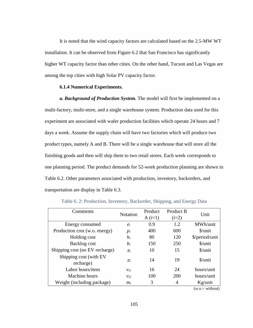
105
It is noted that the wind capacity factors are calculated based on the 2.5-MW WT
installation. It can be observed from Figure 6.2 that San Francisco has significantly
higher WT capacity factor than other cities. On the other hand, Tucson and Las Vegas are
among the top cities with high Solar PV capacity factor.
6.1.4 Numerical Experiments.
a. Background of Production System. The model will first be implemented on a
multi-factory, multi-store, and a single warehouse system. Production data used for this
experiment are associated with wafer production facilities which operate 24 hours and 7
days a week. Assume the supply chain will have two factories which will produce two
product types, namely A and B. There will be a single warehouse that will store all the
finishing goods and then will ship them to two retail stores. Each week corresponds to
one planning period. The product demands for 52-week production planning are shown in
Table 6.2. Other parameters associated with production, inventory, backorders, and
transportation are display in Table 6.3.
Table 6. 2: Production, Inventory, Backorder, Shipping, and Energy Data
Comments Notation
Product
A (i=1)
Product B
(i=2) Unit
Energy consumed ei 0.9 1.2 MWh/unit
Production cost (w.o. energy) pi 400 600 $/unit
Holding cost hi 80 120 $/period/unit
Backlog cost bi 150 250 $/unit
Shipping cost (no EV recharge) i 10 15 $/unit
Shipping cost (with EV
recharge) i 14 19 $/unit
Labor hours/item vi1 16 24 hours/unit
Machine hours vi2 100 200 hours/unit
Weight (including package) mi 3 4 Kg/unit
(w.o.= without)

106
Table 6. 3: Product demand for 52-week planning
Store 1 Store 2 Store 1 Store 2
Week A B A B Week A B A B
1 798 430 748 513 27 692 469 616 514
2 721 563 710 584 28 740 595 659 594
3 770 552 674 422 29 643 518 674 592
4 793 497 719 442 30 688 583 670 575
5 763 510 798 525 31 690 544 797 470
6 736 463 792 524 32 647 579 600 433
7 755 448 787 460 33 721 506 749 522
8 796 600 756 412 34 696 596 698 546
9 760 427 723 597 35 786 414 629 505
10 753 533 662 573 36 731 517 731 490
11 737 563 759 449 37 658 431 650 585
12 791 593 760 425 38 642 527 710 410
13 776 503 751 462 39 708 589 688 481
14 796 572 634 575 40 785 445 768 402
15 729 564 760 503 41 631 583 669 590
16 740 476 705 415 42 677 576 727 455
17 723 524 782 426 43 747 468 799 569
18 783 536 765 556 44 747 549 725 538
19 795 457 809 520 45 707 534 791 411
20 799 584 799 528 46 603 481 685 479
21 798 407 789 514 47 638 407 786 444
22 756 424 718 515 48 776 474 773 528
23 701 522 622 555 49 741 430 769 445
24 659 447 658 401 50 798 531 795 515
25 730 440 748 437 51 764 492 799 531
26 650 535 672 600 52 707 400 737 430
E-trucks are employed to transport finished goods between the factories, the
warehouse, and the retail stores. The self-weight of each vehicle wv = 5,000 kg, and the
electric vehicle energy intensity rate is qv =1.19×10⁻⁷ MWh/kg/km. The electric load for
warehouse is relatively stable with Lw = 9 MW and the electric load for each retail store
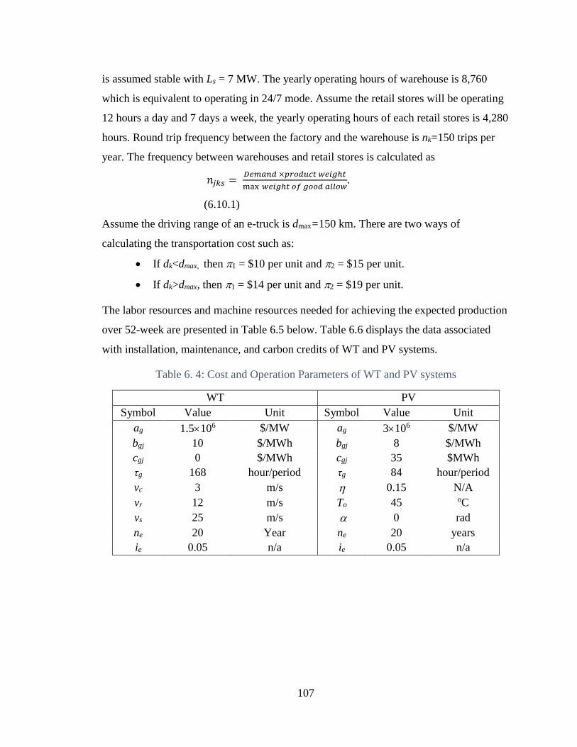
107
is assumed stable with Ls = 7 MW. The yearly operating hours of warehouse is 8,760
which is equivalent to operating in 24/7 mode. Assume the retail stores will be operating
12 hours a day and 7 days a week, the yearly operating hours of each retail stores is 4,280
hours. Round trip frequency between the factory and the warehouse is nk=150 trips per
year. The frequency between warehouses and retail stores is calculated as
𝑛𝑗𝑘𝑠 = 𝐷𝑒𝑚𝑎𝑛𝑑 ×𝑝𝑟𝑜𝑑𝑢𝑐𝑡 𝑤𝑒𝑖𝑔ℎ𝑡
max 𝑤𝑒𝑖𝑔ℎ𝑡 𝑜𝑓 𝑔𝑜𝑜𝑑 𝑎𝑙𝑙𝑜𝑤.
(6.10.1)
Assume the driving range of an e-truck is dmax=150 km. There are two ways of
calculating the transportation cost such as:
• If dk<dmax, then 1 = $10 per unit and 2 = $15 per unit.
• If dk>dmax, then 1 = $14 per unit and 2 = $19 per unit.
The labor resources and machine resources needed for achieving the expected production
over 52-week are presented in Table 6.5 below. Table 6.6 displays the data associated
with installation, maintenance, and carbon credits of WT and PV systems.
Table 6. 4: Cost and Operation Parameters of WT and PV systems
WT PV
Symbol Value Unit Symbol Value Unit
ag 1.5106 $/MW ag 3106 $/MW
bgj 10 $/MWh bgj 8 $/MWh
cgj 0 $/MWh cgj 35 $MWh
τg 168 hour/period τg 84 hour/period
vc 3 m/s 0.15 N/A
vr 12 m/s To 45 oC
vs 25 m/s 0 rad
ne 20 Year ne 20 years
ie 0.05 n/a ie 0.05 n/a

108
Table 6. 5: Labor and Machine Resources in the Factory
Labor Resource Machine Resource
Week Factory 1 Factory 2 Factory 1 Factory 2
1 31051 22486 213179 174419
2 27757 20099 186767 152810
3 26985 19541 182749 149522
4 27580 19972 190130 155562
5 29572 21414 199900 163554
6 26776 21402 206365 168845
7 27462 19885 190702 156029
8 28851 20892 200268 163856
9 29219 21159 199872 163531
10 29820 21594 205161 167859
11 27200 19696 183586 150206
12 28669 20760 201326 164721
13 28374 21553 200405 163967
14 29000 22006 205609 168226
15 26646 19295 183815 150394
16 27947 22251 211605 173131
17 27341 19799 198336 150903
18 27063 19598 200125 152366
19 24881 18491 196036 171766
20 30384 22002 206544 168991
21 30156 23850 209258 182583
22 31399 22736 216919 177479
23 23273 16852 164413 134520
24 28129 20369 189791 155284
25 25368 18370 176176 144144
26 24711 17895 167513 137055
27 30523 22102 213710 174854
28 28786 22857 214837 175775
29 26076 18883 181580 148565
30 27864 20177 190584 155933
31 29679 21492 201714 165039
32 28218 20434 192369 157392
33 25926 18775 182831 149589
34 29941 21681 205688 168290
35 29656 21474 204147 167029
36 24578 17798 170760 139713
37 25508 18470 173099 141627
38 22974 16637 159123 130192
39 27088 19616 184791 151192
40 27191 19689 190750 156068
41 26029 20863 182001 162558
42 26403 19119 181884 148813
43 28747 20817 197046 161219
44 26310 19053 183505 150141
45 27775 20113 190762 156078

109
b. Result Analysis and Discussion. AMPL optimization software was used to test
the model of P4. Using CPLEX solver running in AMD Radeon R6 processor, the model
is tested in different cities with different weather conditions. The production level at both
factories, inventory level, and backlogs for Products A and B in 52 weeks are shown in
Figures 6.4 and 6.5.
Figure 6. 4: Decision Variables Output of Product A
Figure 6. 5: Decision Variables Output of Product B
0
200
400
600
800
1000
1200
1400
1600
0 10 20 30 40 50
Qu
anti
ty
Week
Production, Inventory, Backlog for Product A
Factory 1
Factory 2
Inventory
Backlog
0
100
200
300
400
500
600
700
800
900
0 10 20 30 40 50 60
Axi
s Ti
tle
Axis Title
Production, Inventory, Backlog for Product B
Factory 1
Factory 2
Inventory
Backlog

110
There are two case scenarios which are set up to test the model. The cities chosen
to set up the factory facilities, warehouse, and stores are based on its weather conditions,
cost metrics, demand size, and logistic factors. Figures 6.6 and 6.7 show the layouts of
two scenarios with distances.
Figure 6. 6: Scenario I Supply Chain layout
Figure 6. 7: Scenario II layout
c. Scenarios with carbon credits. In these scenarios, the cost to install WT system
is $1.5M/MW and the cost to install PV system is $3M/MW. Due to the high PV

111
installation costs, carbon credits of $35/MWh are considered for PV system. Table 6.6
displays the result of Production-Logistics systems of two scenarios with carbon credits.
Table 6. 6: Results of Production-Logistics Systems -Two Scenarios
Scenario I Scenario II
Type
Capacity
(MW) Type
Capacity
(MW)
Factory 1 - Yuma WT 63.01 Factory 1 - Phoenix WT 92.47
Factory 2 - Tucson WT 48.01 Factory 2 - Reno WT 50.64
Warehouse - Los
Angeles WT 76.95
Warehouse - Las
Vegas WT 43.47
Store 1 -
Sacramento WT 20.36
Store 1 - Salt Lake
City WT 16.48
Store 2 - San
Francisco WT 7.01 Store 2 - San Jose WT 39.05
Annualized system
cost $86,868,199.16
Annualized system
cost $86,699,242.84
In scenario one, the minimum total cost of production, transportation, inventory,
and energy is $86,868,199. Even though Yuma and Tucson which are known for their
strong sun and medium wind speed are chosen for factory location, the model still
chooses to install WT systems despite the given carbon credit of $35/MWh for PV’s.
This can be explained because even if Yuma and Tucson have strong sun, it is still more
economical to install the wind turbine due to its low-cost in comparison to PV. Due to its
strong wind , the capacity of WT at San Francisco is lower if compared to other store
locations.
In scenario II, the minimum total cost of production, transportation, inventory,
and energy is $ 86,699,242. Given the carbon credit of $35 MWh, the model still chooses
to install WT systems in all locations. If Comparing all the factory locations, Tucson is

112
the best location to build the factory due to its lowest capacity requirement for WT
system. As for the warehouse locations, Las Vegas is the choice since it only requires
43.47 MW of WT system capacity which is significantly lower than Los Angeles. For
retail store locations, San Francisco is the best location with very low capacity
requirement for WT system dues to its strong wind.
d. Scenarios without carbon credits. Due to the driving forces of policy and
market, the price of solar energy has declined significantly to the point where solar
generation can compete with wind energy. In these scenarios, the installation price of
both WT and PV system will be set at $1.5M/MW. There will be no carbon credits
considered since the cost of PV system is low. Table 6.7 displays the result of
Production-Logistics systems of two scenarios under the new setting.
Table 6. 7: Results of Production-Logistics System without Carbon Credits
Scenario III Scenario IV
Type Capacity
(MW) Type
Capacity
(MW)
Factory 1 - Yuma PV 52.29 Factory 1 - Phoenix PV 67.75
Factory 2 - Tucson PV 37.13 Factory 2 - Reno WT 49.34
Warehouse - Los
Angeles WT 76.95
Warehouse - Las
Vegas WT 43.47
Store 1 - Sacramento WT 20.36 Store 1 - Salt Lake
City WT 16.48
Store 2 - San
Francisco WT 7.01 Store 2 - San Jose WT 39.05
Annualized system
cost $83,997,900.00
Annualized system
cost $83,407,400.00
For scenario III, the total minimum cost of production, inventory, transportation,
and energy is $83,997,900.00. Since the cost of WT system and PV system are set to be
the same, the model chooses PV system for both Yuma and Tucson. This result is

113
predictable since the two cities have strong sunshine. Then, the capacity required for
onsite system at Yuma and Tucson in this scenario is also smaller than scenario I. As for
other locations, the outputs are the same for all of them as the model choose WT systems.
The total cost of scenario III is lower than the total cost of scenario I because the capacity
required for the onsite system of both factories is lower in scenario III.
For scenario IV, the total minimum cost of production, inventory, transportation,
inventory, and energy is $83,407,400.00. With the same capacity cost for WT and PV
system, the model chooses PV system for the Phoenix factory and chooses WT for all
other locations. Since Phoenix has strong sun, it is understandable that the model chooses
PV as the onsite power unit. The total cost of scenario IV is slightly lower than the total
cost of scenario II because the capacity required for onsite system is lower than scenario
two.
6.1.5 Multi-Warehouse Supply Chain Systems
a. System Setting and Parameters. In this section Problem P4 is solved with
four-factories, two-warehouses, and four-retailers. In this setting, Phoenix, Reno, Yuma,
and Tucson are chosen for factory locations, and Los Angeles and Las Vegas are chosen
for the warehouse locations. Salt Lake City, San Jose, Sacramento, and San Francisco are
dedicated to retail store locations. The supply chain layout can be observed from Figure
6.8 which include the distances between sites.

114
Figure 6. 8: Supply Chain Layout with Distance for Travel
All four factories can produce Products A and B to meet the demand of four retail
stores and finished products are transported to warehouse in Las Vegas and Los Angeles
using e-trucks. The parameters of WT and PV remain the same as in Chapter 4 when
performing the numerical experiment. Table 6.8 shows the demand for four factories
where Factory 1 = Phoenix, Factory 2 = Reno, Factory 3= Yuma, and Factory 4= Tucson.
Table 6.9 shows the labor and machine resources available for four factories.

115
Table 6. 8: Product Demand for 52 Weeks
Store 1 Store 2 Store 3 Store 4
Week
Product
A
Product
B
Product
A
Product
B
Product
A
Product
B
Product
A
Product
B
1 698 430 748 513 723 490 724 484
2 791 563 710 584 714 443 684 469
3 670 552 674 422 760 587 639 599
4 753 497 619 442 613 595 726 482
5 763 510 748 525 615 444 664 575
6 656 463 642 524 800 467 629 409
7 715 448 647 460 751 571 771 548
8 636 600 606 412 721 469 642 488
9 660 427 723 597 665 440 645 410
10 703 533 662 573 777 531 622 572
11 737 563 759 449 692 503 706 513
12 791 593 760 425 785 538 758 421
13 726 503 751 462 663 557 680 420
14 796 572 634 575 650 446 767 460
15 729 564 800 503 748 581 635 546
16 740 476 605 415 681 464 660 447
17 773 524 782 426 622 565 646 481
18 623 536 705 556 606 583 790 541
19 795 457 799 520 656 558 646 580
20 749 584 609 528 782 534 618 501
21 778 407 749 514 724 566 637 451
22 706 424 758 515 687 593 790 574
23 701 522 622 555 689 519 602 521
24 659 447 658 401 795 507 761 590
25 730 440 748 437 794 592 667 404
26 650 535 672 600 625 474 629 557
27 672 469 616 514 781 494 689 408
28 740 595 689 594 602 445 753 466
29 643 518 674 592 693 416 662 419
30 628 583 670 575 798 525 667 477
31 690 544 797 470 681 547 739 421
32 647 579 600 433 614 424 754 593
33 721 506 749 522 757 583 670 501
34 606 596 718 546 755 494 765 544
35 786 414 629 505 694 512 772 578
36 731 517 731 490 650 597 754 450
37 658 431 650 585 661 493 667 514
38 642 527 710 410 796 563 718 588
39 708 589 688 481 613 439 653 568
40 795 445 768 402 783 437 742 466
41 631 583 669 590 703 583 688 588
42 677 576 727 455 615 513 718 589
43 747 468 799 569 756 528 708 567
44 747 549 725 538 703 491 745 480
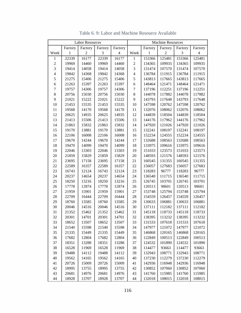
116
Table 6. 9: Labor and Machine Resource Available
Labor Resources Machine Resources
Week
Factory
1
Factory
2
Factory
3
Factory
4 Week
Factory
1
Factory
2
Factory
3
Factory
4
1 22339 16177 22339 16177 1 153366 125481 153366 125481
2 19969 14460 19969 14460 2 134365 109935 134365 109935
3 19414 14058 19414 14058 3 131474 107570 131474 107570
4 19842 14368 19842 14368 4 136784 111915 136784 111915
5 21275 15406 21275 15406 5 143813 117665 143813 117665
6 21263 15397 21263 15397 6 148464 121471 148464 121471
7 19757 14306 19757 14306 7 137196 112251 137196 112251
8 20756 15030 20756 15030 8 144078 117882 144078 117882
9 21021 15222 21021 15222 9 143793 117648 143793 117648
10 21453 15535 21453 15535 10 147598 120762 147598 120762
11 19568 14170 19568 14170 11 132076 108062 132076 108062
12 20625 14935 20625 14935 12 144839 118504 144839 118504
13 21413 15506 21413 15506 13 144176 117962 144176 117962
14 21863 15832 21863 15832 14 147920 121026 147920 121026
15 19170 13881 19170 13881 15 132241 108197 132241 108197
16 22106 16008 22106 16008 16 152234 124555 152234 124555
17 19670 14244 19670 14244 17 132688 108563 132688 108563
18 19470 14099 19470 14099 18 133975 109616 133975 109616
19 22046 13303 22046 13303 19 151033 123573 151033 123573
20 21859 15829 21859 15829 20 148593 121576 148593 121576
21 23695 17158 23695 17158 21 160545 131355 160545 131355
22 22589 16357 22589 16357 22 156057 127683 156057 127683
23 16743 12124 16743 12124 23 118283 96777 118283 96777
24 20237 14654 20237 14654 24 136540 111715 136540 111715
25 18250 13216 18250 13216 25 126745 103701 126745 103701
26 17778 12874 17778 12874 26 120513 98601 120513 98601
27 21959 15901 21959 15901 27 153748 125794 153748 125794
28 22709 16444 22709 16444 28 154559 126457 154559 126457
29 18760 13585 18760 13585 29 130633 106881 130633 106881
30 20046 14516 20046 14516 30 137111 112182 137111 112182
31 21352 15462 21352 15462 31 145118 118733 145118 118733
32 20301 14701 20301 14701 32 138395 113232 138395 113232
33 18652 13507 18652 13507 33 131533 107618 131533 107618
34 21540 15598 21540 15598 34 147977 121072 147977 121072
35 21335 15449 21335 15449 35 146868 120165 146868 120165
36 17682 12804 17682 12804 36 122849 100513 122849 100513
37 18351 13288 18351 13288 37 124532 101890 124532 101890
38 16528 11969 16528 11969 38 114477 93663 114477 93663
39 19488 14112 19488 14112 39 132943 108771 132943 108771
40 19562 14165 19562 14165 40 137230 112279 137230 112279
41 20726 15009 20726 15009 41 142936 116948 142936 116948
42 18995 13755 18995 13755 42 130852 107060 130852 107060
43 20681 14976 20681 14976 43 141760 115985 141760 115985
44 18928 13707 18928 13707 44 132018 108015 132018 108015

117
b. Results Analysis. The model has total of 848 decision variables which include
production level for each factory, inventory for each warehouse, and backorders as well
as the onsite power capacity of WT and PV in each facility. Figure 6.9 shows the results
of the production quantity of Product A at all factories that meet the deterministic
demand per week. Figure 6.10 displays the inventory-backorder level of Product A for all
warehouses. Figure 6.11 shows the result of the production quantity for Product B in all
the factories. Figure 6.12 displays the inventory backorder level of Product B for all
warehouses across 52 periods or weeks.
Figure 6. 9: Production Quantity of Product A
0
200
400
600
800
1000
1200
1400
0 1 0 2 0 3 0 4 0 5 0
QU
AN
TITY
WEEK
PRODUCTION QUANTITY OF PRODUCT A
Factory 1 Factory 2 Factory 3 Factory 4

118
Figure 6. 10: Inventory-Backorder Level of Product A
Figure 6. 11: Production Quantity of Product B
0
50
100
150
200
250
0 1 0 2 0 3 0 4 0 5 0
QU
AN
ITY
WEEK
INVENTORY-BACKORDER LEVEL FOR PRODUCT A
Inventory Warehouse 1 Inventory Warehouse 2 Backorder 1 Backorder 2
0
100
200
300
400
500
600
700
800
0 1 0 2 0 3 0 4 0 5 0 6 0
QU
AN
TITY
WEEK
PRODUCTION QUANTITY OF PRODUCT B
Factory 1 Factory 2 Factory 3 Facotry 4

119
Figure 6. 12: Inventory- Backorder Level of Product B
The results of the optimization of the onsite generation capacity are presented in
two cases and summarized in Table 6.10. In the first case, the installation cost of WT
system is set at $1.5M/MW and the installation cost of PV system is set at $3M/MW.
Since the cost of PV is high, carbon credits are considered. In the second case, the cost of
installation is the same as $1.5M/MW and there will be no carbon credits.
0
100
200
300
400
500
600
0 1 0 2 0 3 0 4 0 5 0
QU
AN
TITY
WEEK
INVENTORY-BACKORDER OF PRODUCT B
Inventory of Product 1 Inventory of Warehouse 2 Backorder 2 Backorder 2

120
Table 6. 10: Comparison under Different PV cost and Carbon Credits
Case 1 Case 2
PV Capacity Cost
($/MW) 3,000,000 1,500,000
WT Capacity Cost
($/MW) 1,500,000 1,500,500
PV Carbon Credits 35 0
Type
Capacity
(MW) Type
Capacity
(MW)
Factory 1 WT 129.92 PV 97.67
Facotry 2 WT 72.68 WT 68.17
Factory 3 WT 93.27 PV 78.84
Factory 4 WT 69.97 PV 52.74
Warehouse 1 WT 43.81 WT 43.81
Warehouse 2 WT 77.5 WT 77.5
Retail Store 1 WT 16.58 WT 16.58
Retial Store 2 WT 39.2 WT 39.2
Retial Store 3 WT 20.48 WT 20.48
Retail Store 4 WT 7.05 WT 7.05
Annualized total cost
$
165,438,000.00
$
156,577,000.00
In Case 1 where the PV system cost is higher than WT system, the model chooses
to install WT system for all facilities even though carbon credits are applied for PV. The
annualized total cost for Case 1 is $156,577,000.00. For the factory locations, Tucson has
the lowest capacity requirements of 69.97 MW due to its medium wind speed. On the
other hand, Phoenix has the highest capacity of 129.92 MW. For the retail store locations,
San Francisco has the lowest wind capacity requirement of 7.05 MW and San Jose has
the highest wind capacity requirement of 39.2 MW.
In Case 2 the installation cost of PV and WT is the same with no carbon credits, the
model returns a different result than Case 1. The model chooses to install PV system for
Phoenix, Yuma, and Tucson locations. Furthermore, the capacity requirement for the PV
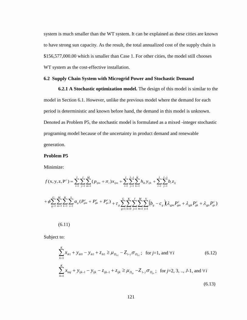
121
system is much smaller than the WT system. It can be explained as these cities are known
to have strong sun capacity. As the result, the total annualized cost of the supply chain is
$156,577,000.00 which is smaller than Case 1. For other cities, the model still chooses
WT system as the cost-effective installation.
6.2 Supply Chain System with Microgrid Power and Stochastic Demand
6.2.1 A Stochastic optimization model. The design of this model is similar to the
model in Section 6.1. However, unlike the previous model where the demand for each
period is deterministic and known before hand, the demand in this model is unknown.
Denoted as Problem P5, the stochastic model is formulated as a mixed -integer stochastic
programing model because of the uncertainty in product demand and renewable
generation.
Problem P5
Minimize:
=
−
==
−
= == = =
+++=I
i
J
j
iji
I
i
J
j
K
k
ijkik
I
i
J
j
M
m
ijmiijm
c zbyhxpf1
1
11
1
1 11 1 1
)()P,z,y,x(
= = = =
+++G
g
M
m
K
k
S
s
c
gs
c
gk
c
gmg PPPa1 1 1 1
)( ( )= = = = =
++−+G
g
K
k
J
j
M
m
S
s
c
gsgjs
c
gkgjk
c
gmgjmggg PPPcb1 0 1 1 1
)(
(6.11)
Subject to:
11 1110
1
1 isis DDikikik
K
k
ik Zzyyx −
=
−+−+ ; for j=1, and i (6.12)
ijsijs DDijkijkijkijk
K
k
imj Zzzyyx −−−
=
−+−−+ 111
1
; for j=2, 3, .., J-1, and i
(6.13)

122
iJiJ DDiJiJiJ
K
kiJ Zzyyx −−−
=
−−−+ 1111
; for j=J, and i (6.14)
ljm
I
i
ijmilm wxv =1
, for i and j (6.15)
𝑧𝑖𝑘,𝐽 = 0 for i and k (6.16)
= == =
=++J
j
G
g
c
gmgjmg
v
mmkv
I
i
J
j
ijmimmkvim Pwdnqxmdnqe1 11 1
)( (6.17)
= == = ==
=+++J
j
G
g
c
gkgjkg
I
i
J
j
S
s
sjksv
v
ijsi
J
j
v
mmkvww PdnqwDmwdnqLt1 11 1 11
)( (6.18)
= ==
=+J
j
G
g
c
gsg
J
j
v
sjksvss PwdnqLt1 11
(6.19)
0,, c
gs
c
gk
c
gu PPP , for g, k, u, s (6.20)
xijm, yijk, zijk are non-negative integers (6.21)
6.2.2 Numerical experiments.
a. Multi-factory, multi-store, and single warehouse model. First the supply chain
of the multi-factory, single warehouse, and multi-store network is implemented in the
model. The model will have the same setting as the one in Chapter 5 with two factories
producing two product types, namely product A and product B. The demand for each
product in each week is uncertain but given that they will follow the normal distribution.
The mean demands and standard deviations for each week in each factory are listed
below in Table 6.11. The other parameters associated with production, inventory, and
backorders, and transportation will be the same as the deterministic model.

123
Table 6. 11: Production Demand
Product 1 Product 2
Facility Mean Standard
Deviation Mean
Standard
Deviation
Store 1 706 56 508 60
Store 2 709 62 500 62
i. Result Analysis and Discussion. The production quantity, inventory level, and
backlogs for both Products A and B in 52 weeks for Case I are displayed in Figures 6.13
and 6.14. For Case II, the production-inventory results are shown by Figures 6.15 and
6.16. Notice that the model is solved with confidence level of =0.9 to meet the
production demands.
Figure 6. 13: Production Output of Product A for Case I
0
200
400
600
800
1000
1200
1400
1600
1800
0 1 0 2 0 3 0 4 0 5 0
QU
AN
TITY
WEEK
OUTPUT OF PRODUC A FOR CASE I
Factory 1 Factory 2 Inventory Backorder

124
Figure 6. 14: Production Output of Product B for Case I
Figure 6. 15: Production Output of Product A for Case I
0
200
400
600
800
1000
1200
1400
0 1 0 2 0 3 0 4 0 5 0 6 0
QU
AN
TITY
WEEK
OUTPUT OF PRODUCT B FOR CASE I
Factory 1 Factory 2 Inventory Backorder
0
200
400
600
800
1000
1200
1400
1600
1800
0 1 0 2 0 3 0 4 0 5 0
QU
AN
TITY
WEEK
OUTPUT OF PRODUCT A FOR CASE II
Factory 1
Factory 2
Inventory
Backorder

125
Figure 6. 16: Production Output of Product B for Case II
Two scenarios are considered to test the model in which the network layouts are
similar to the deterministic model (Section 6.1.4). In Case 1, Phoenix, Arizona and Reno,
Nevada are chosen to set up the manufacturing facilities while warehouse is located in
Las Vegas, NV. Retail stores will be located in Salt Lake City, UT and San Jose, CA.
Case 2 will have the factories located in Yuma, AZ and Tucson, AZ. The warehouse
location is in Los Angeles, CA while retail stores are located at Sacramento, CA and San
Francisco, CA. The layout of both cases and the travel distances can be observed in
Figures 6.17 and 6.18 below.
0
100
200
300
400
500
600
700
800
900
1000
0 1 0 2 0 3 0 4 0 5 0
QU
AN
TITY
WEEK
OUTPUT OF PRODUCT B FOR CASE II
Factory 1
Factory 2
Inventory
Backorder

126
Figure 6. 17: Case 1 Supply Chain Network
Figure 6. 18: Case 2 Supply Chain Network
ii. The Cases with Carbon Credits. For these runs, the cost of WT system
installation is $1.5M/MW and the cost of PV system installation is $3M/MW. Carbon
credits are also considered for PV system dues to its high installation cost. The output of
decision variables of two cases with carbon credits is displayed in Table 6.12.

127
Table 6. 12: Results of Production-Logistics Systems of Two Cases
Case I Case II
Type Capacity
(MW) Type
Capacity
(MW)
Factory 1 - Phoenix WT 98.81 Factory 1 - Yuma WT 72.76
Factory 2 - Reno WT 59.55 Factory 2 - Tucson WT 49.68
Warehouse - Las
Vegas WT 43.36
Warehouse - Los
Angeles WT 76.78
Store 1 - Salt Lake
City WT 16.45 Store 1 - Sacramento WT 20.35
Store 2 - San Jose WT 38.96 Store 2 - San Francisco WT 7
Annualized
system cost $92,295,600.00
Annualized
system cost $91,983,300.00
In Case I, the annualized total cost of production, transportation, inventory, and
energy is $92,295,600 and for Case II is $91,983,300. As expected, the model chooses to
install WT system for all its locations despite of carbon credits of $35/MWh being
applied to PV. Compared with deterministic model (see Table 6.7 of Section 6.1.4), it can
be seen that capacity requirements for all the locations in the stochastic model are very
similar to the deterministic model.
iii. The Cases without Carbon Credits. For this run, the installation cost for both
WT and PV systems are set at $1.5M/MW. Since the cost for both systems are low,
carbon credits will not be applied to PV. Table 6.13 shows the result of running the
model for the Production-Logistics system under two cases and without carbon credits.

128
Table 6. 13: Capacity Output of Two Cases without Carbon Credits
Case I Case II
Type Capacity
(MW) Type
Capacity
(MW)
Factory 1 - Phoenix PV 78.25 Factory 1 - Yuma PV 55.87
Factory 2 - Reno WT 51.05 Factory 2 - Tucson WT 42.91
Warehouse - Las Vegas WT 43.36 Warehouse - Los Angeles WT 76.78
Store 1 - Salt Lake City WT 16.45 Store 1 - Sacramento WT 20.35
Store 2 - San Jose WT 38.96 Store 2 - San Francisco WT 7
Annualized system cost $88,601,700.00 Annualized system cost $88,836,500.00
In this test, the model chooses to install PV system for facilities located in
Phoenix, Tucson, and Yuma. Since these cities have strong sun capability, the capacity
requirements for onsite generation system are much lesser compared to the WT system if
chosen. The PV capacity requirement is 21 percent less than the WT capacity
requirement for Phoenix, 23.21 percent in Yuma, and 13.63 percent in Tucson. As the
result, the annualized total costs are lower than the previous test. For Case 1, the
annualized total cost is $88,601,700, and for Case II, the annualized total cost is
$88,836,500.
b. Multi-warehouse supply chain system. Using the same setting, this
Section presents the results of solving Problem P5 for a multi-warehouse supply chain
system under deterministic demand. The supply chain network will include four-
factories, two-warehouses, and four-retail stores. Figure 6.19 shows the layout of the
supply chain network and the distance between destinations. Table 6.14 shows the mean
production demand and standard deviation of all the factories.

129
Figure 6. 19: Supply Chain Layout with Distance Travel
Table 6. 14: Mean and Standard Deviation of Demand for Product A and Product B
Facility Product A Product B
Mean Stdv Mean Stdv
Store 1 780 50 740 45
Store 2 809 51 760 60
Store 3 850 60 780 62
Store 4 810 62 700 55
i. Result Analysis. In this test, the model also has total of 848 decision variables
and more than 500 constraints. Figure 6.20 indicates the output of the production quantity
for product A at all factories that meet the uncertain demand of each week. Figure 6.21
displays the inventory-backorders level of product A for all warehouses. Figure 6.22
shows the result of the production quantity for Product B at all factories.

130
Figure 6. 20: Production Output for Product A
Figure 6. 21: Production Output for Product B
0
200
400
600
800
1000
1200
1400
0 1 0 2 0 3 0 4 0 5 0 6 0
QU
AN
TITY
WEEK
PRODUCTION OUTPUT OF PRODUCT A
Factory 1
Factory 2
Factory 3
Factory 4
0
100
200
300
400
500
600
700
800
900
0 1 0 2 0 3 0 4 0 5 0 6 0
QU
AN
TITY
WEEK
PRODUCTION OUTPUT OF PRODUCT B
Factory 1
Factory 2
Factory 3
Factory 4

131
Figure 6. 22: Inventory-Backorder level for Product B
The results of the optimization of onsite generation capacity are presented in two
cases and summarized in Table 6.16. In the first case, the installation cost of WT system
is set at $1.5M/MW and the installation cost of PV system is set at $3M/MW. Since the
cost of PV is high, carbon credits are considered. In Case 2, the cost of installation is the
same as $1.5M/MW and there will be no carbon credits.
0
50
100
150
200
250
300
350
400
0 10 20 30 40 50
Qu
anti
ty
Week
Inventory -Backorder for Product 2
Warehouse 1
Warehouse 2
Backorder 1
Backorder 2

132
Table 6. 15: Optimization of Onsite Generation Capacity
Case 1 Case 2
PV Capacity Cost
($/MW) 3,000,000 1,500,000
WT Capacity Cost
($/MW) 1,500,000 1,500,500
PV Carbon Credits 35 0
Type Capacity
(MW) Type
Capacity
(MW)
Factory 1 WT 119 PV 91.12
Factory 2 WT 72.57 WT 66.04
Factory 3 WT 93.35 PV 78.82
Factory 4 WT 69.89 PV 52.91
Warehouse 1 WT 43.42 WT 43.42
Warehouse 2 WT 46.91 WT 76.91
Retail Store 1 WT 16.45 WT 16.45
Retail Store 2 WT 38.96 WT 38.96
Retail Store 3 WT 20.35 WT 20.35
Retail Store 4 WT 7 WT 7
Annualized total cost $148,952,000.00 $140,476,000.00
It can be observed that the annualized total cost of Case 2 is lower than the cost of
Case 1 and the difference of the cost is 5.69 percent. In Case 1, since the cost of PV
system is twice as high of the WT system, the model chooses to install a WT system to
optimize the operation cost. However, in Case 2 where the capacity costs of WT and PV
system are the same, it is more economical to install PV system dues to the strong sun
capacity of the cities.
133
VII. CONCLUSIONS AND FUTURE WORK
Under the concept of inter-connected microgrid operation, this thesis proposes to
integrate onsite renewables into a multi-site production-logistics system for attaining net-
zero energy performance. The goal is to determine the production, inventory, backorders,
and renewables capacity in each facility such that the total cost is minimized. To tackle
the problem, we propose a renewable generation analytics framework in which over
80,000 meteorological data are collected, classified and analyzed to extrapolate the power
capacity factors under various climate conditions.
Our study contributes to the production and supply chain literature in two aspects.
First, we present a quantitative model to analyze the feasibility and cos-effectiveness of
realizing net-zero energy production-logistics operation using onsite renewable
generation. The thesis introduces two types of models: deterministic model and stochastic
model. The deterministic model can be applied in the industry where the demands are
known or relatively stable in each period while the stochastic model can be used in the
industry where the demands are uncertain or unpredictable. The proposed renewable
generation analytics methodology allows the planner to transform a complex stochastic
programming problem into a two-stage deterministic optimization model.
As the second contribution, manufacturing facilities have long been treated as
energy consumers. This thesis makes an early attempt to convert the manufacturers into a
“prosumer” who can produce and consume energy concurrently. Eighteen cities that
cover a wide range of wind and weather profiles are chosen to test and verify the
proposal model. The experiments show that achieving net-zero energy operation is
affordable in regions where the ground wind speed is above 5 m/s or the overcast days in

134
a year are less than 50%. The study also shows that PV can compete with wind
generation only if its capacity cost is down to $1.5M/MW or its power efficiency
increases to 30% (which is equivalent to reducing the cost by a half).
Future work can be expanded to a globalized production logistics supply chain
with different transportation modes, such as electric trains. Another extension of the
model can be incorporating battery storage systems into the microgrid system. An energy
storage system by which excess power produced by WT or PV system can be stored
locally to hedge against the periods when the wind profile and solar radiation are weak.
As a result, the facilities can avoid importing electricity from the main grid when there is
no wind or solar power available. Last, but not the least, with the growing deployment of
electric vehicle fleet, there exist plentiful opportunities for the inter-operation between
the electrical vehicles and the local microgrid systems through V2G and G2V operations
in transactive energy market mechanism. In conjunction with demand response, these
emerging technologies will be incorporated into the production and logistics model as the
future research.

135
APPENDIX SECTION
APPENDIX A Single Facility Plus Warehouse and E-Transport with Deterministic
Demand Optimization Programing
set TYPE; # WT or PV #set parameters param T > 0; param C > 0; param cap_fact {1..T, TYPE} >= 0; #factory location capacity param wh_cap {1..T, TYPE} >=0; #warehouse location capacity param demand_prod {i in 1..T, p in 1..C} >= 0; #production demand param labor_dem {1..T} >= 0; # labor resources param machi_dem {1..T} >= 0; #machine resources param cost_prod {1..C} >= 0; #production cost param cost_hold {1..C} >= 0; #holding cost param cost_back {1..C} >= 0; #backlog cost param res_labor {1..C} >=0; #labor hourly cost param res_mach {1..C} >=0; #machine hourly cost param ins_cost {TYPE}>= 0; #installation cost param om_cost{TYPE} >= 0; #operation and maintenance cost param carbon_credit{TYPE} >= 0; #carbon credit param eng_consume{1..C} >= 0; #energy consumed per product type param oper_hrs{TYPE} >= 0; #operation hours param cap_recover >= 0; #capital recovery param e_ware >= 0; #energy consumed by warehouse param inv0; #initial inventory level param back0; #initial backlog level param distance >=0; #distance travel param freq >= 0; #travel frequency param w_goods >= 0; #weight of goods param w_vehicle >= 0;#weight of vehicle param density >= 0; #Define variable var prod_month {1..T, 1..C} >= 0; #production level var hold_month { 0..T, 1..C} >= 0; #inventory level var back_month { 0..T, 1..C} >=0; #backlog level var capacity {j in TYPE}>=0; #factory capacity var wh_capacity{j in TYPE}>=0; # warehouse capacity #Calculate Production Cost var ProductionC= sum {i in 1..T, p in 1..C} cost_prod[p]*prod_month[i,p]; #calculate inventory cost var Inventory= sum {i in 1..T,p in 1..C} cost_hold[p] * hold_month[i,p]; #calaculate backorder cost var Backorder=

136
sum {i in 1..T, p in 1..C} cost_back[p] * back_month[i,p]; #calculate installation, operation and maintenance cost, and carbon credits for factory# var IntFact= sum {j in TYPE} capacity[j] * ins_cost[j]*cap_recover; var OmFact = sum {i in 1..T,j in TYPE } capacity[j] * om_cost[j] * cap_fact[i,j]*oper_hrs[j]; var Credit_fact= sum {i in 1..T, j in TYPE } capacity[j] * carbon_credit[j] * cap_fact[i,j]*oper_hrs[j]; #calculate installation, operation and maintenance cost, and carbon credits for factory# var IntWare = sum {j in TYPE} wh_capacity[j] * ins_cost[j]*cap_recover ; var OmWare = sum {i in 1..T, j in TYPE } wh_capacity[j] * om_cost[j] * wh_cap[i,j]*oper_hrs[j]; var Credit_ware = sum {i in 1..T, j in TYPE } wh_capacity[j] * carbon_credit[j] * wh_cap[i,j]*oper_hrs[j]; #Objective Function minimize total_cost: ProductionC + Inventory + Backorder + IntFact+OmFact - Credit_fact + IntWare + OmWare - Credit_ware; #Constraints #Energy balance for factory subject to Requirement : (sum {i in 1..T,p in 1..C} prod_month[i,p] * eng_consume[p])+ density*distance*freq*(w_goods+w_vehicle) = (sum{i in 1..T,j in TYPE} cap_fact[i,j]*capacity[j]*oper_hrs[j]); #Energy balance for warehouse subject to Warehouse: sum{i in 1..T,j in TYPE} wh_cap[i,j]*wh_capacity[j]*oper_hrs[j]= 8760*e_ware + density*distance*freq*(w_vehicle); #initial inventory and backlog subject to Init_hold{p in 1..C}: hold_month[0,p] = inv0; subject to Init_back{p in 1..C}: back_month[0,p] = back0; #production and demand equity subject to Production { i in 1..T, p in 1..C}: prod_month[i,p] + hold_month[i-1,p] + back_month[i,p] = demand_prod[i,p]+ hold_month[i,p] + back_month[i-1,p] ; #balancing labor resources subject to LaborDemand {i in 1..T}: sum{ p in 1..C} prod_month[i,p] * res_labor[p] <= labor_dem [i];
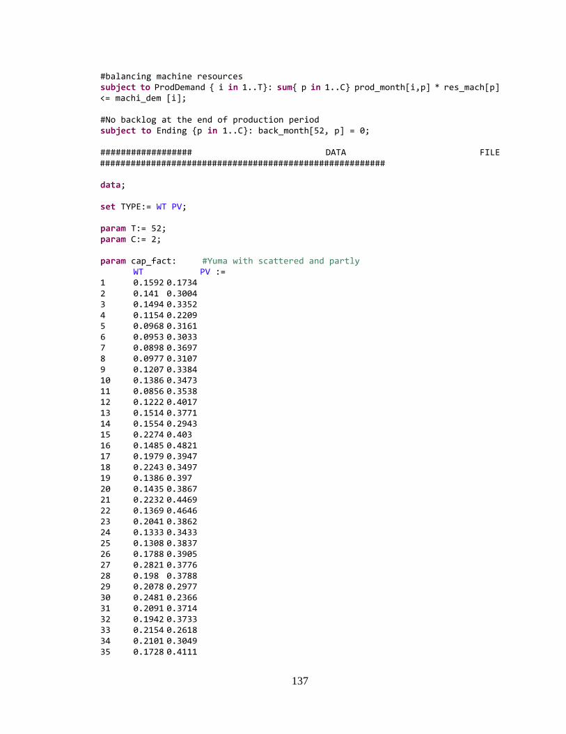
137
#balancing machine resources subject to ProdDemand { i in 1..T}: sum{ p in 1..C} prod_month[i,p] * res_mach[p] <= machi_dem [i]; #No backlog at the end of production period subject to Ending {p in 1..C}: back_month[52, p] = 0; ################## DATA FILE ######################################################## data; set TYPE:= WT PV; param T:= 52; param C:= 2; param cap_fact: #Yuma with scattered and partly WT PV := 1 0.1592 0.1734 2 0.141 0.3004 3 0.1494 0.3352 4 0.1154 0.2209 5 0.0968 0.3161 6 0.0953 0.3033 7 0.0898 0.3697 8 0.0977 0.3107 9 0.1207 0.3384 10 0.1386 0.3473 11 0.0856 0.3538 12 0.1222 0.4017 13 0.1514 0.3771 14 0.1554 0.2943 15 0.2274 0.403 16 0.1485 0.4821 17 0.1979 0.3947 18 0.2243 0.3497 19 0.1386 0.397 20 0.1435 0.3867 21 0.2232 0.4469 22 0.1369 0.4646 23 0.2041 0.3862 24 0.1333 0.3433 25 0.1308 0.3837 26 0.1788 0.3905 27 0.2821 0.3776 28 0.198 0.3788 29 0.2078 0.2977 30 0.2481 0.2366 31 0.2091 0.3714 32 0.1942 0.3733 33 0.2154 0.2618 34 0.2101 0.3049 35 0.1728 0.4111

138
36 0.1986 0.2471 37 0.1152 0.3361 38 0.0753 0.4437 39 0.0717 0.4028 40 0.1187 0.4093 41 0.0749 0.4392 42 0.0998 0.4089 43 0.1011 0.4154 44 0.0793 0.3426 45 0.1088 0.3427 46 0.1103 0.3324 47 0.0834 0.2952 48 0.088 0.2404 49 0.1346 0.2365 50 0.091 0.2857 51 0.1197 0.2588 52 0.137 0.2494 ; param wh_cap: #San Francisco WT PV := 1 0.1261 0.1399 2 0.118 0.1972 3 0.1286 0.1829 4 0.1407 0.0892 5 0.16 0.0813 6 0.2054 0.1935 7 0.2773 0.1129 8 0.2408 0.191 9 0.2961 0.2102 10 0.3447 0.2232 11 0.3757 0.1554 12 0.402 0.1851 13 0.4784 0.2091 14 0.4645 0.1622 15 0.5848 0.2483 16 0.4926 0.3127 17 0.615 0.2414 18 0.5643 0.2475 19 0.6652 0.2039 20 0.6212 0.2585 21 0.6948 0.2986 22 0.5806 0.1725 23 0.6561 0.2881 24 0.6406 0.2597 25 0.6303 0.3001 26 0.5577 0.2387 27 0.5641 0.2801 28 0.5813 0.2673 29 0.54 0.2409 30 0.5455 0.2421 31 0.5475 0.2016 32 0.5006 0.2583
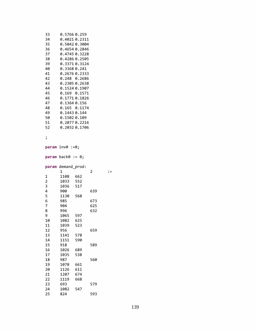
139
33 0.5766 0.259 34 0.4021 0.2311 35 0.5042 0.3004 36 0.4654 0.2846 37 0.4745 0.3228 38 0.4286 0.2505 39 0.3371 0.3124 40 0.3368 0.241 41 0.2676 0.2333 42 0.248 0.2686 43 0.2305 0.2638 44 0.1524 0.1907 45 0.169 0.1571 46 0.1771 0.1826 47 0.1364 0.156 48 0.165 0.1174 49 0.1443 0.144 50 0.1502 0.109 51 0.2077 0.2216 52 0.2032 0.1706 ; param inv0 :=0; param back0 := 0; param demand_prod: 1 2 := 1 1108 662 2 1033 552 3 1036 517 4 900 639 5 1130 568 6 985 673 7 904 625 8 996 632 9 1065 597 10 1082 625 11 1039 523 12 956 659 13 1141 578 14 1151 590 15 918 589 16 1026 689 17 1035 538 18 987 560 19 1078 661 20 1126 611 21 1207 674 22 1119 668 23 693 579 24 1082 547 25 824 593
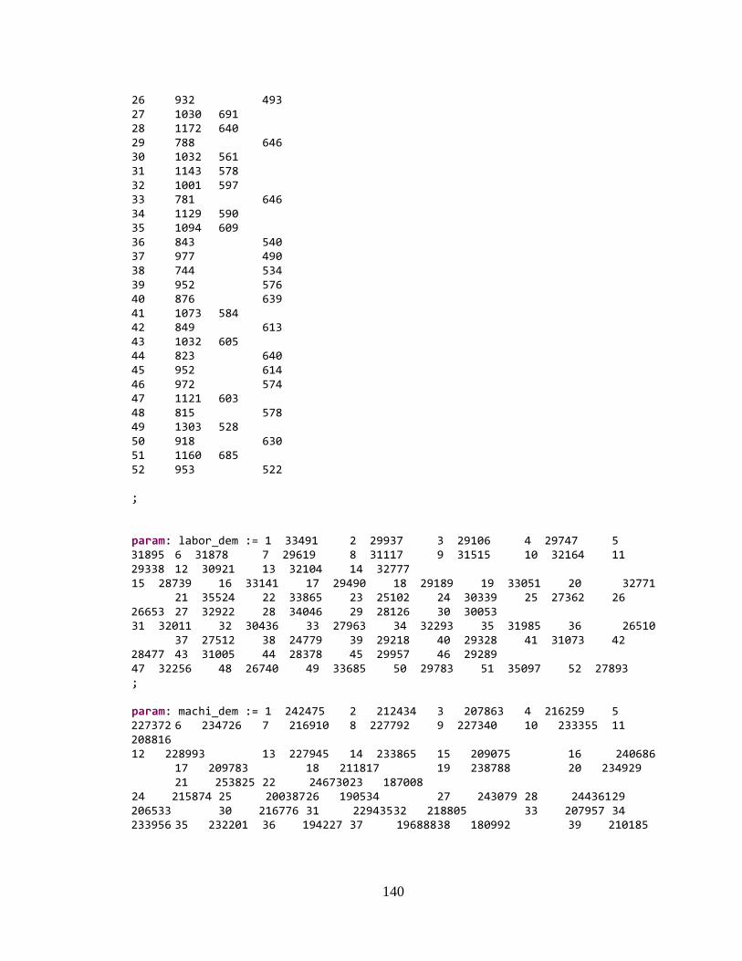
140
26 932 493 27 1030 691 28 1172 640 29 788 646 30 1032 561 31 1143 578 32 1001 597 33 781 646 34 1129 590 35 1094 609 36 843 540 37 977 490 38 744 534 39 952 576 40 876 639 41 1073 584 42 849 613 43 1032 605 44 823 640 45 952 614 46 972 574 47 1121 603 48 815 578 49 1303 528 50 918 630 51 1160 685 52 953 522 ; param: labor_dem := 1 33491 2 29937 3 29106 4 29747 5 31895 6 31878 7 29619 8 31117 9 31515 10 32164 11 29338 12 30921 13 32104 14 32777 15 28739 16 33141 17 29490 18 29189 19 33051 20 32771 21 35524 22 33865 23 25102 24 30339 25 27362 26 26653 27 32922 28 34046 29 28126 30 30053 31 32011 32 30436 33 27963 34 32293 35 31985 36 26510 37 27512 38 24779 39 29218 40 29328 41 31073 42 28477 43 31005 44 28378 45 29957 46 29289 47 32256 48 26740 49 33685 50 29783 51 35097 52 27893 ; param: machi_dem := 1 242475 2 212434 3 207863 4 216259 5 227372 6 234726 7 216910 8 227792 9 227340 10 233355 11 208816 12 228993 13 227945 14 233865 15 209075 16 240686 17 209783 18 211817 19 238788 20 234929 21 253825 22 246730 23 187008 24 215874 25 200387 26 190534 27 243079 28 244361 29 206533 30 216776 31 229435 32 218805 33 207957 34 233956 35 232201 36 194227 37 196888 38 180992 39 210185
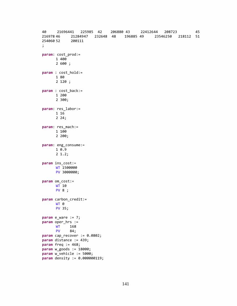
141
40 216964 41 225985 42 206880 43 224126 44 208723 45 216978 46 212849 47 232648 48 196885 49 235462 50 218112 51 254060 52 200111 ; param: cost_prod:= 1 400 2 600 ; param : cost_hold:= 1 80 2 120 ; param : cost_back:= 1 200 2 300; param: res_labor:= 1 16 2 24; param: res_mach:= 1 100 2 200; param: eng_consume:= 1 0.9 2 1.2; param ins_cost:= WT 1500000 PV 3000000; param om_cost:= WT 10 PV 8 ; param carbon_credit:= WT 0 PV 35; param e_ware := 7; param oper_hrs := WT 168 PV 84; param cap_recover := 0.0802; param distance := 439; param freq := 468; param w_goods := 18000; param w_vehicle := 5000; param density := 0.000000119;

142
APPENDIX B: Getting Wind Data from WeatherUnderground Using R Code
library(weatherData)
#get station airport code
getStationCode("Reno", region = "Nevada")
#get wind data for 11 year from 2006 to 2016
year2016<-getSummarizedWeather(station_id = 'KTUS', start_date = '2016-01-01',
end_date = '2016-12-31', station_type = "airportCode",opt_temperature_columns =
FALSE, opt_all_columns =FALSE, opt_custom_columns = TRUE, custom_columns =
c(18))
year2015<-getSummarizedWeather(station_id = 'KTUS', start_date = '2015-01-01',
end_date = '2015-12-31', station_type = "airportCode",opt_temperature_columns =
FALSE, opt_all_columns =FALSE, opt_custom_columns = TRUE, custom_columns =
c(18))
year2014<-getSummarizedWeather(station_id = 'KTUS', start_date = '2014-01-01',
end_date = '2014-12-31', station_type = "airportCode", opt_temperature_columns
= FALSE, opt_all_columns =FALSE, opt_custom_columns = TRUE, custom_columns =
c(18))
year2013<-getSummarizedWeather(station_id = 'KTUS', start_date = '2013-01-01',
end_date = '2013-12-31', station_type = "airportCode",opt_temperature_columns =
FALSE, opt_all_columns =FALSE, opt_custom_columns = TRUE, custom_columns =
c(18))
year2012<-getSummarizedWeather(station_id = 'KTUS', start_date = '2012-01-01',
end_date = '2012-12-31', station_type = "airportCode", opt_temperature_columns
= FALSE, opt_all_columns =FALSE, opt_custom_columns = TRUE, custom_columns =
c(18))
year2011<-getSummarizedWeather(station_id = 'KTUS', start_date = '2011-01-01',
end_date = '2011-12-31', station_type = "airportCode",opt_temperature_columns =
FALSE, opt_all_columns =FALSE, opt_custom_columns = TRUE, custom_columns =
c(18))
year2010<-getSummarizedWeather(station_id = 'KTUS', start_date = '2010-01-01',
end_date = '2010-12-31', station_type = "airportCode",opt_temperature_columns =
FALSE, opt_all_columns =FALSE, opt_custom_columns = TRUE, custom_columns =
c(18))
year2009<-getSummarizedWeather(station_id = 'KTUS', start_date = '2009-01-01',
end_date = '2009-12-31', station_type = "airportCode",opt_temperature_columns =
FALSE, opt_all_columns =FALSE, opt_custom_columns = TRUE, custom_columns =
c(18))
year2008<-getSummarizedWeather(station_id = 'KTUS', start_date = '2008-01-01',
end_date = '2008-12-31', station_type = "airportCode", opt_temperature_columns
= FALSE, opt_all_columns =FALSE, opt_custom_columns = TRUE, custom_columns =
c(18))
year2007<-getSummarizedWeather(station_id = 'KTUS', start_date = '2007-01-01',
end_date = '2007-12-31', station_type = "airportCode",opt_temperature_columns =
FALSE, opt_all_columns =FALSE, opt_custom_columns = TRUE, custom_columns =
c(18))
year2006<-getSummarizedWeather(station_id = 'KTUS', start_date = '2006-01-01',
end_date = '2006-12-31', station_type = "airportCode",opt_temperature_columns =

143
FALSE, opt_all_columns =FALSE, opt_custom_columns = TRUE, custom_columns =
c(18))
library(rowr)
weather <-cbind.fill(year2016, year2015, year2014, year2013, year2012, year2011,
year2010, year2009, year2008, year2007, year2006)
write.csv(weather, "Tucson.csv")
data <- read.csv("Tucson.csv")
#print(data)
data <- data[,!(colnames(data) %in%
c("Date","Date.1","Date.2","Date.3","Date.4","Date.5","Date.6","Date.7","Date.
8","Date.9","Date.10"))]
write.csv(data, "Tucson.csv")
library(xlsx)
#install.packages('plyr')
library(plyr)
dat<-read.csv("Tucson.csv")
y16 = xtabs(~ Week + Year2016, dat)
y15 = xtabs(~ Week + Year2015, dat)
y14 = xtabs(~ Week + Year2014, dat)
y13 = xtabs(~ Week + Year2013, dat)
y12 = xtabs(~ Week + Year2012, dat)
y11 = xtabs(~Week + Year2011, dat)
y10 = xtabs(~ Week + Year2010, dat)
y9 = xtabs(~ Week + Year2009, dat)
y8 = xtabs(~ Week + Year2008, dat)
y7 = xtabs(~ Week + Year2007, dat)
y6 = xtabs(~ Week + Year2006, dat)
weather<-cbind(y16,y15,y14,y13,y12,y11,y10,y9,y8,y7,y6)
write.csv (weather, "Tucson_sun.csv")
144
REFERENCES
A. Pham, T. Jin, C. Novoa, C. Temponia, “Minimizing levelized cost of distributed wind
and solar power: Toward zero carbon supply chain operations,” INFORMS, October 20-
25, 2017, Houston, TX.
Annual Report-REN21, (2016), “REN100 Annual Report 2016”. The Climate Group.
Media.virbcdn.com. Web. February 26, 2016. Available at http://www.ren21.net/ren21-
annual-report-2016/, (access on March 25, 2017).
Accordino, M. H., Rajagopal, D., (2015), “When a national cap-and-trade policy with a
carve-out provision may be Preferable to a national CO2 tax.” Energy Journal, vol. 36,
no. , pp. 189-207. Sustainability Reference Center Webpage. (accessed on 15 May 2016).
Armstong, A., (2015), “Clean energy in manufacturing: Gaining ground in the U.S.”
Renewable Energy World. Renewableenergyworld.com. November 2, 2015. (accessed on
February 25, 2016).
Ball, P.D., Evans, S., Ellison, D., (2009), “Zero carbon manufacturing facility:Towards
integrating material, energy and waste process flows,” Journal of Engineering
Manufacture, vol. 223, no. 9, Part B, pp. 1085-1096.
Binkley, D., Stephen Harsh, Christopher A. Wolf, Steven Safferman, Dana Kirk, (2013),
“Electricity purchase agreements and distributed energy policies for anaerobic digesters,”
Energy Policy, Volume 53, February 2013, Pages 341-352.
Blackadar, A. K., H. Tennekes, (1968), “Asymptotic similarity in neutral, barotropic,
atmospheric boundary layers,” Journal of Atmospheric Sciences, vol. 25, no. 11, pp.
10151020.
BMW. “Annual Account Press Conference 2015” (PDF). Retrieve 30 September 2016.
BMW. “Annual Report 2015” (PDF). Retrieved 2 October 2016.
BMW. “Sustainable Value Report 2015” (PDF).Retrieved 30 September 2016
Botsford, C. and A. Szczepanek., (2009) "Fast Charging Vs. Slow Charging: Pros and
Cons for the New Age of Electric Vehicles." 24Th International Battery, Hybrid and Fuel
Cell Electric Vehicle Symposium and Exhibition 2009, EVS 24, vol. 3, no. 24th

145
International Battery, Hybrid and Fuel Cell Electric Vehicle Symposium and Exhibition
2009, EVS 24, 01, p. 1811-1819.
Bouchery, Y., Ghaffari, A., Jemai, Z., Dallery, Y., (2012), “Including sustainability
criteria into inventory models,” European Journal of Operational Research, vol. 222, no.
2, pp. 229-240.
Cai, T., S. Duan, C. Chen, (2010), “Forecasting power output for photovoltaic grid
connected power systems without using solar radiation measurement,” in Proceedings of
Power Electronics for Distributed Generation Systems Symposium, pp. 773-777.
Cao, H., H. Li, (2014), “Simulation-based approach to modeling the carbon emissions
dynamic characteristics of manufacturing system considering disturbances,” Journal of
Cleaner Production, vol. 64, no. 2, pp. 572-580.
Daclison-Dickey, R., (2013), “100 electric vehicles begin their journey to save 126,000
gallons of fuel per year,” Longitudes, UPS, URL
http://blog.ups.com/2013/02/08/100electric-vehicles-begin-theirjourney-to-save-126000-
gallons-of-fuel-per-year/.
Davidson, C., D. Steinberg, and R. Margolis. (2016), "Exploring the Market For Third-
PartyOwned Residential Photovoltaic Systems: Insights From Lease And Power-
Purchase Agreement Contract Structures And Costs In California." Environmental
Research Letters 10.2 (2015): Scopus®. Web. 21 Sept. 2016.
Edge, P., (2015), "An Approximation of Counterparty Credit Risk in Long Term Power
Purchase Agreements (Ppas)."" International Conference on The European Energy
Market, EEM 2015-August.2015 12th International Conference on the European Energy
Market, EEM 2015 (2015): Scopus®. Web. 20 May 2016.
EPA, (2016), "Overview of Greenhouse Gas". United States Environmental Protection
Agency. Epa.gov. Web February 26, 2016. https://www.epa.gov/ghgemissions/overview-
greenhouse-gases, (accessed on May, 5 2017)
Federgruen, A., Zipkin, P., (1984), “Approximation of dynamic, multi-location
production and inventory problems,” Management Science, vol. 30, no. 1, pp. 69-84.
Forster, P., V. Ramaswamy, P. Artaxo, T. Berntsen, R. Betts, D.W. Fahey, J. Haywood,
J. Lean, D.C. Lowe, G. Myhre, J. Nganga, R. Prinn, G. Raga, M. Schulz and R. van
Dorland, (2007), “Changes in Atmospheric Constituents and in Radiative Forcing,” In:

146
Climate Change 2007: The Physical Science Basis. Contribution of Working Group I to
the Fourth Assessment Report of the Intergovernmental Panel on Climate Change
[Solomon, S., D. Qin, M. Manning, Z. Chen, M. Marquis, K.B. Averyt, M.Tignor and
H.L. Miller (eds.)].Cambridge University Press, Cambridge, United Kingdom and New
York, NY, USA.
Freris, L., Infield, D., (2008), “Renewable Energy in Power Systems”, Chapter 7, John
Wiley & Sons, West Sussex, UK.
Galluci, Maria and Flynn, Kerry, (2016), “How apple is taking the tech world’s love
affair with renewables to a new level”. Mashable. 09 August 2016. Web 01 October
2016.http://mashable.com/2016/08/09/apple-selling-renewable energy/#eG20J84PCZqq
General Motors, (2016), “GM’s Renewable Energy Use Fact Sheet” (PDF). Retrieved 27
September 2016.
General Motors, (2016), “GM 2015 Q4 Chart set, General Motors Company” (PDF).
Retrieved. 27 Sept 2016
General Motors, (2016), “Solar Array at Corvette Plants Drives GM to lead in Solar
Energy Use.” GM Corporate Newsroom. Web. 27 September 2016.
http://media.gm.com/media/us/en/gm/home.detail.html/content/Pages/news/us/en/2015/d
ec/1201-solar.html
Golari, M., Fan, F., Jin, T., (2017), “Multistage stochastic optimization for production
inventory planning with intermittent renewable energy,” Production and Operations
Management, vol. 26, no. 3, pp. 409-425.
Gong, X., Zhou, S.X., (2013), “Optimal production planning with emissions trading,”
Operations Research, vol. 61, no. 4, pp. 908-924.
Greenpeace Australia, Pacific, (2015), "Energy [R]Evolution: A Sustainable World
Energy Outlook 2015." BASE. Web. 15 Mar 2016
Haghifam, M.-R., M. Omidvar, (2006), “Wind farm modeling in reliability assessment of
power system,” in Proceedings of International Conference on Probabilistic Methods
Applied to Power Systems, pp. 1-5.

147
Hammami, R., Nouira, I., Frein, Y., (2015), “Carbon emissions in a multi-echelon
production-inventory model with lead time constraints,” International Journal of
Production Economics, vol. 164, no. 6, pp. 292-307.
Heier, S., (2005), “Grid Integration of Wind Energy: Onshore and Offshore Conversion
Systems”, 3rd Edition, page. 45, John Wiley & Sons, Chichester, UK.
Hickey, B., (2014), “Anheuser-Busch brewing up some wind, solar power,” KCRA News
Archive, August 14, 2014, available at http://www.kcra.com/article/anheuser-
buschbrewing-up-some-wind-solar-power/6416039, (accessed on March 16, 2017).
Higle, J., Kempf, K., (2001), “Production planning under supply and demand
uncertainty: A stochastic programming approach,” in: Stochastic Programming,
International Series in Operations Research & Management Science, Infanger, G. (ed.)
Springer, New York, pp. 297-315.
Hua, G., Cheng, T.C.E., Wang, S., (2011), “Managing carbon footprints in inventory
management,” International Journal of Production Economics, vol. 132, no. 2, pp.
178185.
Koenig, R., (2009), "Power Purchase Agreement Checklist for State and Local
Governments." (2009): SciTech Connect. Web. 1 June 2016.
Krass, Dmitry, Timur Nedorezov, and Anton Ovchinnikov, (2013), "Environmental
Taxes And The Choice Of Green Technology."" Production & Operations Management
22.5 (2013): 1035-1055. Business Source Complete. Web. 20 Sept. 2016.
Labrador, David, (2015), “Lockeed Martin Signs Its First Major Renewables Deal for 30
MW of Lockeed Martin.""Science of Citizenship."" Sustainability Report 2015.
Retrieved. 27 Sept 2016
Lave M., J. Kleissl, (2011), “Optimum fixed orientations and benefits of tracking for
capturing solar radiation,” Renewable Energy, vol. 36, no. 3, pp. 1145-1152.
Lee, H.L., Yano, C.A., (1988), “Production control in multistage systems with variable
yield losses,” Operations Research, vol. 36, no. 2, pp. 269-279.
Leonard, Annie. The Story of Cap & Trade: Annotated Script. The Story of Stuff.
[Online] 2009. [Cited: September 15, 2016.]
148
Letchford, C.W. and B.C. Zachry, (2009), "On Wind, Waves, and Surface Drag." 5Th
European and African Conference on Wind Engineering, EACWE 5, Proceedings, no.
5th European and African Conference on Wind Engineering, EACWE 5, Proceedings, 01
Jan. 2009, p. 32p.
Letmathe, P., Balakrishnan, N., (2005), “Environmental considerations on the optimal
product mix,” European Journal of Operational Research, vol. 167, no. 2, pp. 398-412.
Lever-Tracey, Constance, ed. Routledge International Handbooks: Routledged Handbook
of Climate Change and Society (1). Florence, US: Routledge, 2010. ProQuest ebrary.
Web
Li, Lin, et al. ""Optimal Production Scheduling For Energy Efficiency Improvement In
Biofuel Feedstock Preprocessing Considering Work-In-Process Particle Separation.""
Energy 96.(2016): 474-481. ScienceDirect. Web. 20 Sept. 2016.
Lohman, Larry. “Carry on Polluting”. New Scientist. 2006, 2580.
Lozanova, Sarah. “Walmart Leaps Toward 100% Renewable Energy with Wind Deal.”
Triple Pundit. Triple Pundit, 2015. Web 9 October 2015.
Makridou, Georgia, et al. ""A Two-Stage Approach for Energy Efficiency Analysis In
European Union Countries."" Energy Journal 36.2 (2015): 47-69. Sustainability
Reference Center. Web. 19 Sept. 2016.
Martí, Joana M. Comas, Jean-Sébastien Tancrez, and Ralf W. Seifert. "Carbon Footprint
And Responsiveness Trade-Offs in Supply Chain Network Design."" International
Journal of Production Economics 166. (2015): 129-142. ScienceDirect. Web. 21 Sept.
2016.
McKibben, B. "What We Know: The Reality, Risks and Response To Climate Change."
New York Review of Books 61.12 (n.d.): 46-48. Arts & Humanities Citation Index.
Web.30 Feb 2016.
Mekhilef, S., R. Saidur, and A. Safari. ""Review On Solar Energy Use In Industries.""
Renewable And Sustainable Energy Reviews 4 (2011): AGRIS. Web. 5 Dec. 2015.
Mian, Yang, and Yang Fuxia. "Energy-Efficiency Policies and Energy Productivity
Improvements: Evidence From China's Manufacturing Industry."" Emerging Markets
Finance & Trade 52.6 (2016): 1395-1404. Business Source Complete. Web. 14 Sept.
2016.

149
Ming Zeng, Yongqi Yang, Qiannan Fan, Yingxin Liu, Zhuojun Zou, “Coordination
between clean energy generation and thermal power generation under the policy of
“direct power-purchase for large users,” Utilities Policy, Volume 33, April 2015, Pages
10-22.
Mouzon, Gilles, Mehmet B. Yildirim, and Janet Twomey. ""Operational Methods For
Minimization Of Energy Consumption Of Manufacturing Equipment."" International
Journal Of Production Research 45.18/19 (2007): 4247-4271. Business Source Complete.
Web. 20 Sept. 2016.
Mula, J., Poler, R., Garca-Sabater, J.P., Lario, F.C. (2006), “Models for production
planning under uncertainty: A review,” International Journal of Production Economics,
vol. 103, no. 1, pp. 271-285.
NREL, “Distributed generation renewable energy estimate of costs,” National Renewable
Energy Laboratory report. ” 2013, Available at
http://www.nrel.gov/analysis/tech_lcoe_re_cost_est.html, (accessed on May 7, 2015).
Pechmann, A., I. Schöler, and S. Ernst. "Possibilities For CO2-Neutral Manufacturing
With Attractive Energy Costs." Journal Of Cleaner Production (2016): ScienceDirect.
Web. 18 Sept. 2016.
Pham, A., Jin, T., Zong, Z., Qin, J., (2017), “Production and Logistics Planning for Net-
Zero Energy Operation under Demand and Generation Uncertainty,” Texas State
University Working Paper.
Pless, S., Torcellini, P., (2010), “Net-zero energy buildings: A classification system
based on renewable energy supply options,” National Renewable Energy Laboratory
Report, http://netzerofoun,dation.org/docs/NREL, (accessed on March 3, 2017).
Proctor, R., B. Fox, and D. Flynn. "Reserve Trading Within Power Purchase
Agreements."" Proceedings of The DRPT2000. International Conference on Electric
Utility Deregulation & Restructuring & Power Technologies (Cat. No.00EX382) (2000):
137. Publisher Provided Full Text Searching File. Web. 6 Apr 2016.
Quaschining,Volker.Wiley-IEEE: Tenewable Energy and Climate Change (1).
Hobken,GB:Wiley, 2009. ProQuest ebrary Web 2 March 2016
Richard, M.G., (2015), “Tesla's Gigafactory will produce as much renewable energy as it
uses (net zero energy),” Energy/Renewable Energy, available at
http://www.treehugger.com/renewable-energy, (accessed on March 31, 2017).
150
Richard, Schmalensee, et al., (2013), “World Energy Consumption and Carbon Dioxide
Emissions: 1950–2050.” Massachusetts Institute of Technology, Mimeo.: BASE. Web.
30 Feb 2016.
Rogelj, J. (1,2), et al. "Zero Emission Targets as Long-Term Global Goals for Climate
Protection." Environmental Research Letters 10.10 (2015): Scopus®. Web. 28 May 2016.
Roy A., Kedare S.B. and Bandyopadhyay S., (2009), Design of wind power generation
system for industrial application incorporating resource uncertainty, Chemical
Engineering Transactions, 18, 647-652 DOI: 10.3303/CET0918105
Ryuto, Shigenobu, et al., (2016), "Optimal Operation and Management for Smart Grid
Subsumed High Penetration of Renewable Energy, Electric Vehicle, And Battery Energy
Storage System."" International Journal of Emerging Electric Power Systems 17.2
(2016): 173189. Academic Search Complete. Web. 6 May 2016.
Sewalk, Stephen, (2013), "Carbon Tax With Reinvestment Trumps Cap-And- Trade."
Pace Environmental Law Review 30.2 (2013): 580-624. Legal Source. Web. 6 June 2016.
Shafer, Bruce, (2009), "Electrical Wind Generation for Cement Manufacturing, A case
Study: Calportland Mojave Plant's 24 MW Wind Project." IEEE. Print 2009.
Smith, Brad, (2016), “Greener datacenters for a brighter future: Microsoft’s commitment
to renewable energy”. Microsoft Blogs. Microsoft, 2016, Web 19 May 2016.
Smith, Patricia, (2016), “Feeling the Heat”, New York Times, Up Front Magazine, p.
2016. Web. April 1, 2016.
Sverdlik, Yevgeniy, (2013), “Apple reaches 100% renewable energy across all data
centers.” Data Center Dynamics. 21 March 2013. Web 5 October 2016.
http://www.datacenterdynamics.com/content-tracks/design-build/apple-reaches-
100renewable-energy-across-all-data-centers/74708.fullarticle
Tang, L., Meng, Y., Wang, G., Chen, Z. L., Liu, J., Hu, G., Chen, L., Zhang, B., (2014),
“Operations Research transforms Baosteel’s operations. Interfaces,” vol. 44, no. 1, pp.
22-38
Thiringer, T., J. Linders, (1993), “Control by variable rotor speed of a fixed pitch wind
turbine operating in a wide speed range,” IEEE Transactions on Energy Conversion, vol.
8, no. 3, pp. 520-526.

151
Tongdan Jin, An Pham, Clara Novoa, Cecilia Temponi, “A net-zero carbon supply chain
model: Minimizing levelized cost of onsite renewable generation,” Supply Chain Forum:
An International Journal, vol. 18, no. 2, 2017, pp. 49-59.
T. Jin, A. Pham, C. Novoa, C. Temponi, “A net-zero carbon supply chain model:
Minimizing cost of onsite renewable energy,” in Proceedings of Information Systems,
Logistics and Supply Chain, June 1-4, 2016, Bordeaux, France, pp. 1-8.
Tredeau, F., Salameh, Z., (2009), “Evaluation of lithium ion phosphate batteries for
electric vehicles application,” in Proceedings of IEEE Vehicle Power and Propulsion
Conference, pp. 1266-1270.
"U.S Energy Information Administration. International Energy Outlook 2009: World
Energy and economic Outlook.” 2009, Available Online At
http://www.eia.doe.gov/oiaf/ieo/world.html,
http://www.eia.doe.gov/oiaf/ieo/highlights.html,http://www.eia.doe.gov/oiaf/ieo/industria
l.html, http://www.eia.doe.gov/emeu/aer/eh/total.html [Accessed 19.9.16]
Vallee, F., J. Lobry, O. Deblecker, (2007), “Impact of the wind geographical correlation
level for reliability studies,” IEEE Transactions on Power Systems, vol. 22, no. 4, pp.
22322239.
Verge, Jason. “Microsoft’s 175 MW Wind Farm Deal is its Biggest Power Purchase
Agreement to Date.” Data Center Knowledge. Data center knowledge, 2014. Web 15
May 2016.
Villarreal, S., Jimenez, J., Jin, T., Cabrera-Rios, M., (2013), “Designing a sustainable and
distributed generation system for semiconductor wafer fabs,” IEEE Transactions on
Automation Science and Engineering, vol. 10, no. 1, pp. 16-26.
Walmart, (2015), “Walmart’s Approach to Renewable Energy.” Walmart, 2015. Web 15
October 2015.
Wang, Y., Gerchak, Y., (1996), “Periodic review production models with variable
capacity, random yield, and uncertain demand,” Management Science, vol. 42, no. 1, pp.
130-137.
Weekes, S.M., A.S. Tomlin, (2014), “Comparison between the bivariate Weibull
probability approach and linear regression for assessment of the long-term wind energy
resource using MCP. Renewable Energy, vol. 68, no. 8, pp. 529-539.
152
Weekes, S.M., A.S. Tomlin, (2014), “Comparison between the bivariate Weibull
probability approach and linear regression for assessment of the long-term wind energy
resource using MCP. Renewable Energy, vol. 68, no. 8, pp. 529-539.
WU (Weather Underground), (2017), Available at http://www.wunderground.com/.
(Accessed on March 2, 2017).
Wu, C.C., Chang, N.B., (2004), “Corporate optimal production planning with varying
environmental costs: A grey compromise programming approach,” European Journal of
Operational Research, vol. 155, no. 1, pp. 68-95.
Yano, C.A., Lee, H.L. (1995). “Lot sizing with random yields: A review,” Operations
Research, vol. 43, no. 2, pp. 311-334.
Zhang, M., Küçükyavuz, S., Yaman, H., (2012), “A polyhedral study of multiechelon lot
sizing with intermediate demands,” Operations Research, vol. 60, no. 4, pp. 918-935.