modal analysis of mdof systems with proportional damping 8 prop damped modal analysis 2008.pdf ·...
TRANSCRIPT
MEEN 617 – HD 8 Modal Analysis with Proportional Damping. L. San Andrés © 2008 1
Handout 8 Modal Analysis of MDOF Systems with Proportional Damping
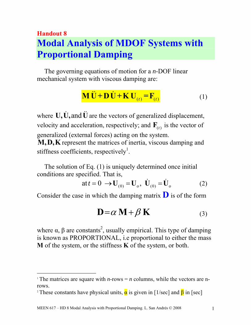
The governing equations of motion for a n-DOF linear mechanical system with viscous damping are:
( ) ( )t tM U + DU +K U =F (1) where andU,U, U are the vectors of generalized displacement, velocity and acceleration, respectively; and ( )tF is the vector of generalized (external forces) acting on the system. M,D,K represent the matrices of inertia, viscous damping and stiffness coefficients, respectively1.
The solution of Eq. (1) is uniquely determined once initial conditions are specified. That is,
(0) (0)at 0 ,o ot = → = =U U U U (2)
Consider the case in which the damping matrix D is of the form
α β= +D M K (3) where α, β are constants2, usually empirical. This type of damping is known as PROPORTIONAL, i.e proportional to either the mass M of the system, or the stiffness K of the system, or both.
1 The matrices are square with n-rows = n columns, while the vectors are n-rows. 2 These constants have physical units, α is given in [1/sec] and β in [sec]

MEEN 617 – HD 8 Modal Analysis with Proportional Damping. L. San Andrés © 2008 2
Proportional damping is rather unique, since only one or two parameters, α, β, appear to fully describe the complexity of damping, irrespective of the system number of DOFs, n. This is clearly not realistic. Hence, proportional damping is not a rule but rather the exception.
Nonetheless the approximation of proportional damping is
useful since, most times damping is quite an elusive phenomenon, i.e. difficult to model (predict) and hard to measure but for a few DOFs.
Next, consider one already has found the natural frequencies
and natural modes (eigenvectors) for the UNDAMPED case, i.e. given M U +K U =0 ,
( ) 1,2...
,i i i nω
=φ satisfying 2
( ) 1,...,i i i nω =⎡ ⎤−⎣ ⎦M +K φ =0 . (4)
with properties [ ] [ ];T TM K= =Φ MΦ Φ KΦ (5)
As in the undamped modal analysis, consider the modal
transformation ( ) ( )t t=U Φ q (6)
And with ( ) ( ) ( ) ( );t t t t= =U Φ q U Φ q , then EOM (1) becomes:
( )t+MΦq + DΦq KΦq =F (7) which offers no advantage in the analysis. However, premultiply the equation above by TΦ to obtain
( ) ( ) ( ) ( )T T T T
t+Φ MΦ q + Φ DΦ q Φ KΦ q =Φ F (8) And using the modal properties, Eq. (5), and
MEEN 617 – HD 8 Modal Analysis with Proportional Damping. L. San Andrés © 2008 3
( )T T T Tα β α β= + = +Φ DΦ Φ M K Φ Φ MΦ Φ KΦ
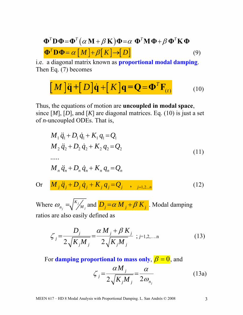
[ ] [ ] [ ]T M K Dα β= + →Φ DΦ (9) i.e. a diagonal matrix known as proportional modal damping. Then Eq. (7) becomes
[ ] [ ] [ ] ( )T
tM D K+ =q + q q =Q Φ F (10) Thus, the equations of motion are uncoupled in modal space, since [M], [D], and [K] are diagonal matrices. Eq. (10) is just a set of n-uncoupled ODEs. That is,
1 1 1 1 1 1 1
2 2 2 2 2 2 2
.....
n n n n n n n
M q D q K q QM q D q K q Q
M q D q K q Q
+ + =+ + =
+ + =
(11)
Or 1,2...,j j j j j j j j nM q D q K q Q =+ + = (12)
Where jjj
KMnω = and j j jD M Kα β= + . Modal damping
ratios are also easily defined as
2 2j j j
jj j j j
D M KK M K M
α βζ
+= = ; j=1,2,….n (13)
For damping proportional to mass only, 0β = , and
22j
jj
nj j
MK Mα αζ
ω= = (13a)

MEEN 617 – HD 8 Modal Analysis with Proportional Damping. L. San Andrés © 2008 4
i.e., the j-modal damping ratio decreases as the natural frequency increases.
For damping proportional to stiffness only, 0α = , (structural damping) and
22jnj
jj j
KK M
βωβζ = = (13b)
i.e., the j-modal damping ratio increases as the natural frequency increases. In other words, higher modes are more increasingly more damped than lower modes. The response for each modal coordinate satisfying the modal Eqn.
1,2...,j j j j j j j j nM q D q K q Q =+ + = proceeds in the same way as for a single DOF system (See Handout 2). First, find initial values in modal space ,
j jo oq q . These follow
from either 1 1;o o o o
− −= =q Φ U q Φ U (14) or
[ ][ ]
1
1
,To o
To o
M
M
−
−
=
=
q Φ M U
q Φ M U (15a)
( ) ( )( ) ( )1 1,
k k
T To k o o k o
k k
q qM M
= =φ M U φ M U (15b)
k=1,….n

MEEN 617 – HD 8 Modal Analysis with Proportional Damping. L. San Andrés © 2008 5
Free response in modal coordinates Without modal forces, Q=0, the modal EOM is
0j j jj H j H j H jM q D q K q Q+ + = = (16)
with solution, for an elastic underdamped mode 1jζ <
( ) ( )( )cos sinj d j
j j j
tH j d j dq e C t S t
ζ ωω ω
−= + if 0
jnω ≠ (17a)
where 21 , jjj j j
KMd n j nω ω ζ ω= − = and
; j j j
j
j
o j n oj o j
d
q qC q S
ζ ω
ω
+= = (17b)
See Handout (2a) for modal responses corresponding to overdamped and critically damped SDOF system. Forced response in modal coordinates
For step-loads, S jQ , the modal equations are
j j j j j j S jM q D q K q Q+ + = (18) with solution, for an elastic underdamped mode 1jζ <
( ) ( )( )cos sinj d j
j j j j
tj d j d Sq e C t S t q
ζ ωω ω
−= + + 0
jnω ≠ (19a)

MEEN 617 – HD 8 Modal Analysis with Proportional Damping. L. San Andrés © 2008 6
where 21 , jjj j j
KMd n j nω ω ζ ω= − = and
( ); ;j j j
j j j
j
S o j n jS j o S j
j d
Q q Cq C q q S
K
ζ ω
ω
+= = − = (19b)
See Handout (2a) for physical responses corresponding to overdamped and critically damped SDOF system. For periodic-loads, Consider the case of force excitation with frequency
jnωΩ ≠ and acting for very long times. The EOMs in physical space are
( )cos t+ ΩPM U + DU K U =F The modal equations are
cos( )
jj j j j j j PM q D q K q Q t+ + = Ω (20) with solutions for an elastic mode, 0
jnω ≠
( ) ( )( )( ) ( )
( )
cos sin
cos sin
j n j
j j
j j
j transient ss t
tj d j d
c s
q q q
e C t S t
C t C t
ζ ωω ω
−
= + =
+ +
Ω + Ω
(21)
The steady state or periodic response is of importance, since the transient response will disappear because of damping dissipative effects. Hence, the j-mode response is:
MEEN 617 – HD 8 Modal Analysis with Proportional Damping. L. San Andrés © 2008 7
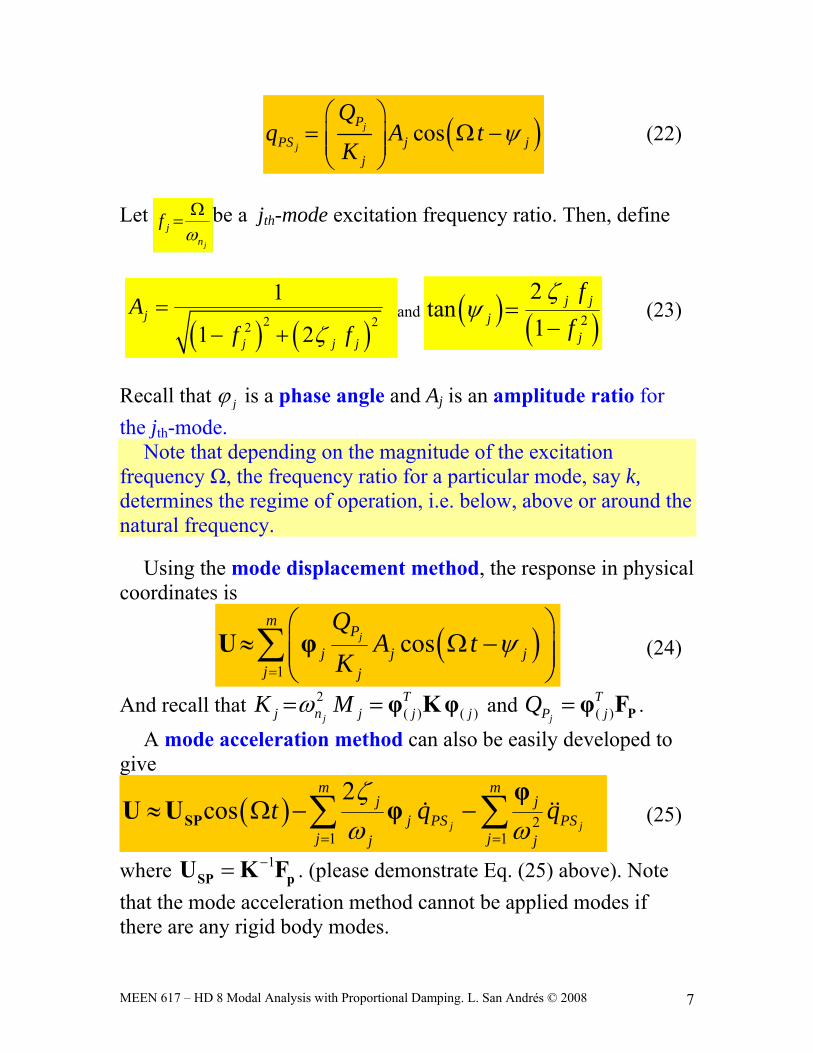
( )cosj
j
PPS j j
j
Qq A t
Kψ
⎛ ⎞= Ω −⎜ ⎟⎜ ⎟⎝ ⎠
(22)
Let
j
jn
fωΩ
= be a jth-mode excitation frequency ratio. Then, define
( ) ( )2 22
1
1 2 j
j j j
Af fζ
=− +
and ( ) ( )2
2tan
1j j
jj
ff
ζψ =
− (23)
Recall that jϕ is a phase angle and Aj is an amplitude ratio for the jth-mode.
Note that depending on the magnitude of the excitation frequency Ω, the frequency ratio for a particular mode, say k, determines the regime of operation, i.e. below, above or around the natural frequency.
Using the mode displacement method, the response in physical coordinates is
( )1
cosjm
Pj j j
j j
QA t
Kψ
=
⎛ ⎞≈ Ω −⎜ ⎟⎜ ⎟
⎝ ⎠∑U φ (24)
And recall that 2( ) ( )j
Tj n j j jK Mω= = φ Kφ and ( )j
TP jQ = Pφ F .
A mode acceleration method can also be easily developed to give
( ) 21 1
2cos
j j
m mj j
j PS PSj jj j
t q qζω ω= =
≈ Ω − −∑ ∑SP
φU U φ (25)
where 1−=SP pU K F . (please demonstrate Eq. (25) above). Note that the mode acceleration method cannot be applied modes if there are any rigid body modes.

MEEN 617 – HD 8 Modal Analysis with Proportional Damping. L. San Andrés © 2008 8
Frequency response functions for damped MDOF systems. The steady state or periodic modal response for j-mode is:
( )cosj
j
PPS j j
j
Qq A t
Kψ
⎛ ⎞= Ω −⎜ ⎟⎜ ⎟⎝ ⎠
(22)
Or, taking the real part of the following complex number expression
j
j
P i tPS j
j
Qq H e
KΩ
⎛ ⎞= ⎜ ⎟⎜ ⎟⎝ ⎠
(26)
where ( ) ( )2
11 2 j
j j j
Hf i fζ
=− +
(27)
with 1i = − is the imaginary unit, and where j
jn
fωΩ
= is the jth-
mode excitation frequency ratio. Then, recall from Eqs. (23)
( ) ( )2 22
1
1 2 j j
j j j
A Hf fζ
=− +
and ( )argj jHψ = (28)
Using the modal transformation, the periodic response UP in
physical coordinates is
( )1
cosjn
Pj j j
j j
QA t
Kψ
=
⎛ ⎞= Ω −⎜ ⎟⎜ ⎟
⎝ ⎠∑PU φ (24)
MEEN 617 – HD 8 Modal Analysis with Proportional Damping. L. San Andrés © 2008 9
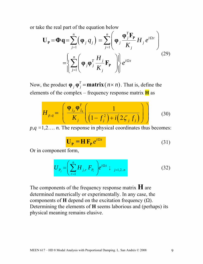
or take the real part of the equation below
( )1 1
1
Tn nj i t
j j j jj j j
njT i t
j jj j
q H eK
He
K
Ω
= =
Ω
=
⎛ ⎞= = = ⎜ ⎟⎜ ⎟
⎝ ⎠⎧ ⎫⎛ ⎞⎪ ⎪= ⎜ ⎟⎨ ⎬⎜ ⎟⎪ ⎪⎝ ⎠⎩ ⎭
∑ ∑
∑
PP
P
φ FU Φq φ φ
φ φ F(29)
Now, the product ( )T
j j n n= ×φ φ matrix . That is, define the elements of the complex – frequency response matrix H as
( ) ( ), 2
11 2
p q
Tj j
p qj j j j
HK f i fζ
⎛ ⎞⎛ ⎞= ⎜ ⎟⎜ ⎟⎜ ⎟⎜ ⎟− +⎝ ⎠⎝ ⎠
φ φ (30)
p,q =1,2…. n. The response in physical coordinates thus becomes:
i te ΩP PU = H F (31)
Or in component form,
, 1,2..1
;j r
ni t
P j r P j nr
U H F e Ω=
=
⎛ ⎞=⎜ ⎟⎝ ⎠∑ (32)
The components of the frequency response matrix H are determined numerically or experimentally. In any case, the components of H depend on the excitation frequency (Ω). Determining the elements of H seems laborious and (perhaps) its physical meaning remains elusive.
MEEN 617 – HD 8 Modal Analysis with Proportional Damping. L. San Andrés © 2008 10
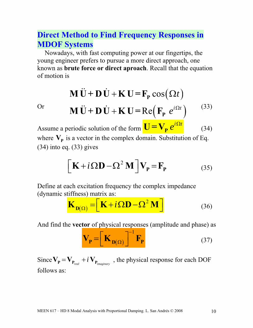
Direct Method to Find Frequency Responses in MDOF Systems
Nowadays, with fast computing power at our fingertips, the young engineer prefers to pursue a more direct approach, one known as brute force or direct aproach. Recall that the equation of motion is
Or
( )( )cos
Re i t
t
e Ω
+ Ω
+
P
P
M U + DU K U =F
M U + DU K U = F (33)
Assume a periodic solution of the form i te Ω
PU = V (34) where PV is a vector in the complex domain. Substitution of Eq. (34) into eq. (33) gives
2i⎡ ⎤+ Ω −Ω =⎣ ⎦ P PK D M V F (35) Define at each excitation frequency the complex impedance (dynamic stiffness) matrix as:
( )2iΩ ⎡ ⎤= + Ω −Ω⎣ ⎦DK K D M (36)
And find the vector of physical responses (amplitude and phase) as
( )
1−
Ω⎡ ⎤= ⎣ ⎦P PDV K F (37)
Since
real imaginaryi= +P P PV V V , the physical response for each DOF
follows as:
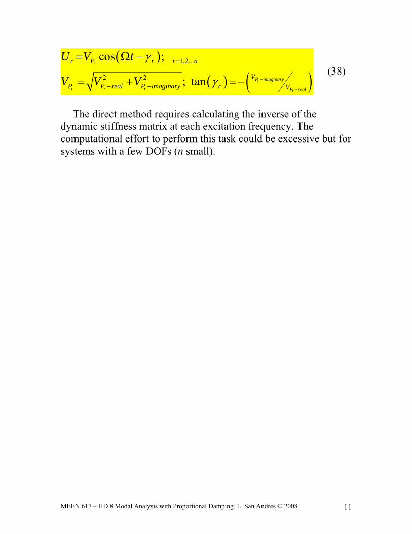
MEEN 617 – HD 8 Modal Analysis with Proportional Damping. L. San Andrés © 2008 11
( )
( ) ( )1,2...
2 2
cos ;
; tan
r
P imaginaryrr r r P realr
r P r r n
VP P real P imaginary r V
U V t
V V V
γ
γ −
−
=
− −
= Ω −
= + =− (38)
The direct method requires calculating the inverse of the
dynamic stiffness matrix at each excitation frequency. The computational effort to perform this task could be excessive but for systems with a few DOFs (n small).

# of DOF
Note M and K are symmetric matrices
example α 0.01s
⋅:= β .001 s⋅:=D α M⋅ β K⋅+:=
D2 103×
1− 103×
1− 103×
2 103×
⎛⎜⎝
⎞⎟⎠N
sm
⋅=
Xo0
0⎛⎜⎝
⎞⎟⎠
m⋅:= Vo0.0
0⎛⎜⎝
⎞⎟⎠
msec
⋅:=initial conditions
Applied force vector: Fo10000
5000−⎛⎜⎝
⎞⎟⎠
N⋅:=
l i
STEP FORCED RESPONSE of 2-DOF mechanical system with proportional damping
ORIGIN 1:=
Dr. Luis San Andres (c) MEEN 363, 617 February 2008
The equations of motion are: (1)M2t
Xdd
2⋅ D
tXd
d⋅+ K X⋅+ Fo=
where M,D, K are matrices of inertia, damping and stiffness coefficients; and X, V=dX/dt,
d2X/dt2 are the vectors of physical displacement, velocity and acceleration, respectively. The FORCED undamped response to the initial conditions, at t=0, Xo,Vo=dX/dt, follows:
For proportional damping, D = α M + β K, so the undamped mode analysis can be used. α & β are physical constants usually determined from measurements of modal damping.
============================================================================================
The equations of motion are:
M11
M21
M12
M22
⎛⎜⎝
⎞⎟⎠ 2t
x1
x2
⎛⎜⎝
⎞⎟⎠
dd
2⋅
D11
D21
D12
D22
⎛⎜⎝
⎞⎟⎠ t
x1
x2
⎛⎜⎝
⎞⎟⎠
dd⋅+
K11
K21
K12
K22
⎛⎜⎝
⎞⎟⎠
x1
x2
⎛⎜⎝
⎞⎟⎠
⋅+F1o
F2o
⎛⎜⎝
⎞⎟⎠
= (2)
1. Set elements of inertia, stiffness & damping matricesDATA FOR problem
M100
0
0
50⎛⎜⎝
⎞⎟⎠
kg⋅:= K2 106⋅
1− 106⋅
1− 106⋅
2 106⋅
⎛⎜⎝
⎞⎟⎠
Nm
⋅:=n 2:=

j 1 n..:=ω j λ j( ) .5:= ω
112.6
217.53⎛⎜⎝
⎞⎟⎠
radsec
= (4)f
ω
2 π⋅:=
f17.92
34.62⎛⎜⎝
⎞⎟⎠Hz=
Note that: Δ ω1( ) Δ ω2( )= 0=
For each eigenvalue, the eigenvectors (natural modes) are
j 1 n..:=Set arbitrarily first element of vector = 1
aj
1
K1 1, M1 1, λ j⋅−
K1 2, M1 2, λ j⋅−( )−
⎡⎢⎢⎢⎣
⎤⎥⎥⎥⎦
:=
a11
0.73⎛⎜⎝
⎞⎟⎠
= a21
2.73−⎛⎜⎝
⎞⎟⎠
= (5)MODAL matrix A j⟨ ⟩ aj:=
A is the matrix of eigenvectors (undampedmodal matrix): each column corresponds to an eigenvector
A1
0.73
1
2.73−⎛⎜⎝
⎞⎟⎠
=
analysis
2. Find eigenvalues (undamped natural frequencies) and eigenvectors
Set determinant of system of eqns = 0
Δ K11 M11 ω2⋅−( ) K22 M22 ω2⋅−( )⋅ K12 M12 ω2⋅−( ) K21 M21 ω2⋅−( )⋅−⎡⎣ ⎤⎦= 0= (2a)
(2b)Δ a ω4⋅ b ω2⋅+ c+= a λ2⋅ b λ⋅+ c+( )= 0= with λ ω2=
where thecoefficientsare:
a M1 1, M2 2,⋅ M1 2, M2 1,⋅−:=(2c)b K1 2, M2 1,⋅ K1 1, M2 2,⋅− K2 2, M1 1,⋅− K2 1, M1 2,⋅+:=
c K1 1, K2 2,⋅ K1 2, K2 1,⋅−:=
The roots of equation (2b) are:
(3)λ1b− b2 4 a⋅ c⋅−( ) .5−⎡⎣ ⎤⎦
2 a⋅:= λ2
b− b2 4 a⋅ c⋅−( ) .5+⎡⎣ ⎤⎦2 a⋅
:=
also known as eigenvalues. The natural frequencies follow as:
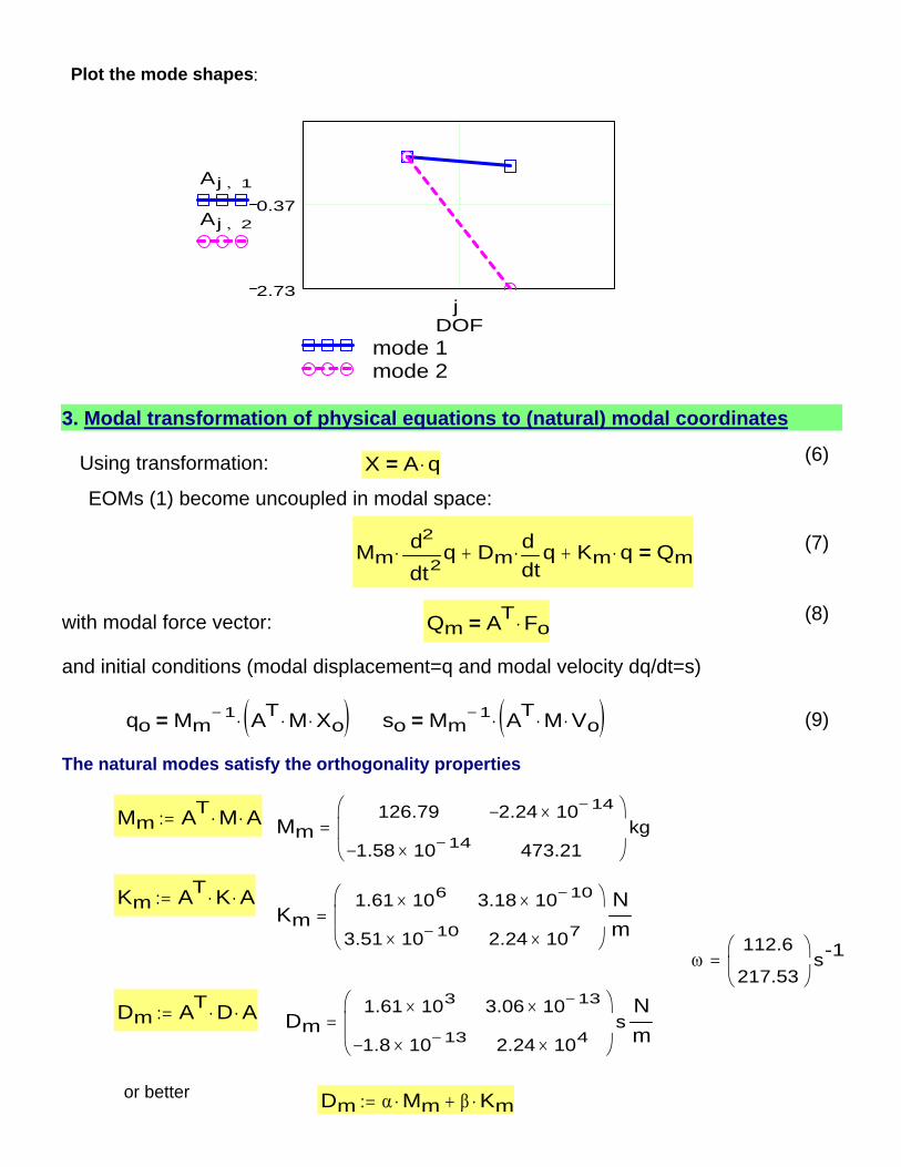
Dm α Mm⋅ β Km⋅+:=or better
Dm1.61 103×
1.8− 10 13−×
3.06 10 13−×
2.24 104×
⎛⎜⎝
⎞⎟⎠s
Nm
=Dm AT D⋅ A⋅:=
ω112.6
217.53⎛⎜⎝
⎞⎟⎠s-1=
Km1.61 106×
3.51 10 10−×
3.18 10 10−×
2.24 107×
⎛⎜⎝
⎞⎟⎠
Nm
=Km AT K⋅ A⋅:=
Mm126.79
1.58− 10 14−×
2.24− 10 14−×
473.21
⎛⎜⎝
⎞⎟⎠kg=Mm AT M⋅ A⋅:=
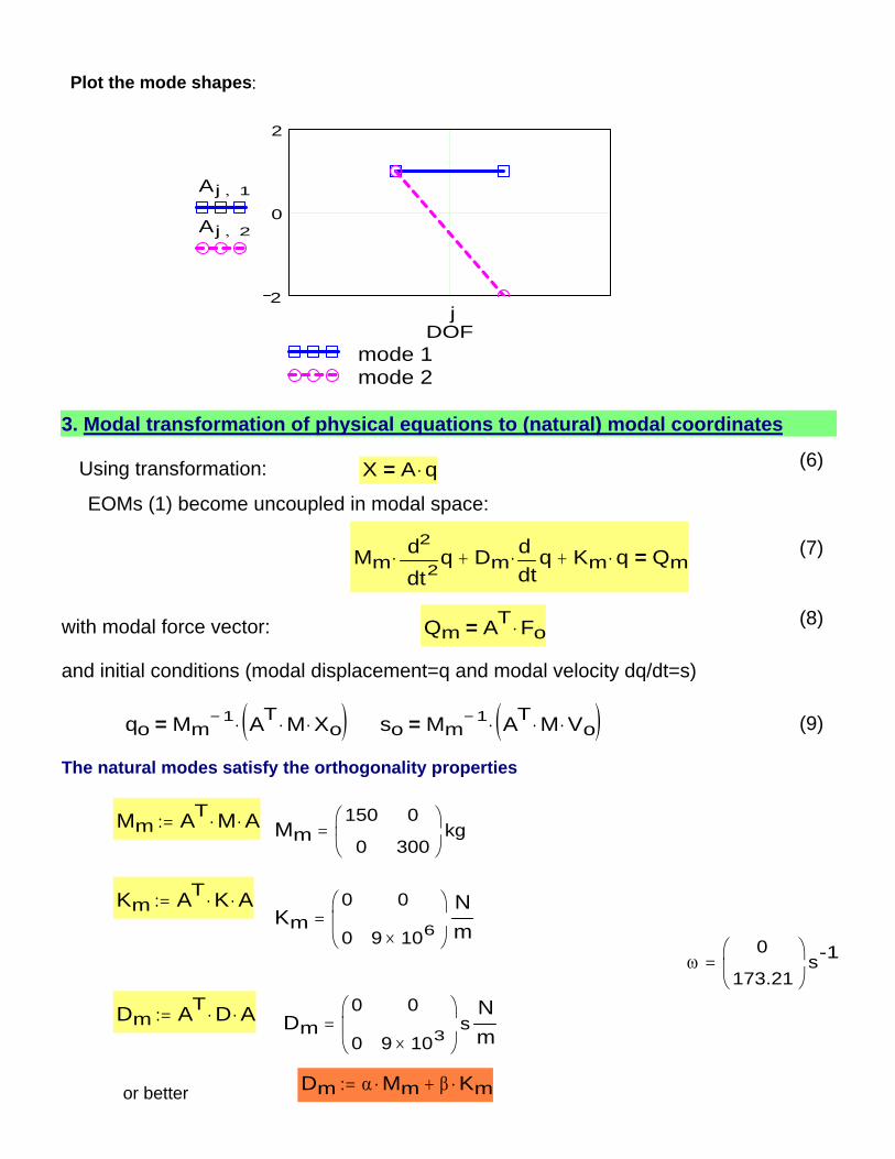
The natural modes satisfy the orthogonality properties
(9)so Mm1− AT M⋅ Vo⋅( )⋅=qo Mm
1− AT M⋅ Xo⋅( )⋅=
and initial conditions (modal displacement=q and modal velocity dq/dt=s)
Qm AT Fo⋅=with modal force vector: (8)
Mm 2tqd
d
2⋅ Dm
tqd
d⋅+ Km q⋅+ Qm= (7)
EOMs (1) become uncoupled in modal space:
X A q⋅=Using transformation: (6)
3. Modal transformation of physical equations to (natural) modal coordinates
2.73
0.37
mode 1mode 2
DOF
Aj 1,
Aj 2,
j
Plot the mode shapes:
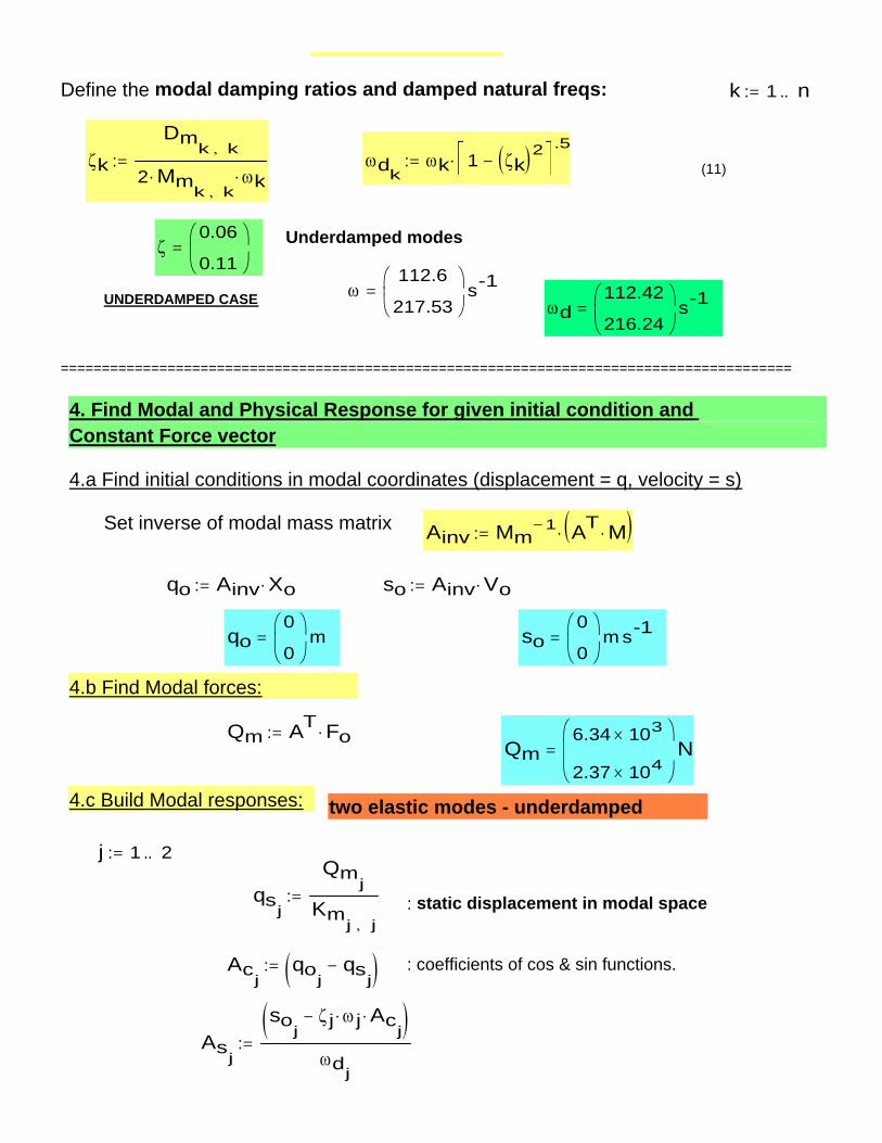
Asj
soj
ζ j ω j⋅ Acj
⋅−( )ωdj
:=
: coefficients of cos & sin functions.Acj
qoj
qsj
−( ):=
: static displacement in modal spaceqsj
Qmj
Kmj j,
:=
j 1 2..:=
two elastic modes - underdamped4.c Build Modal responses:
Qm6.34 103×
2.37 104×
⎛⎜⎝
⎞⎟⎠N=
Qm AT Fo⋅:=
4.b Find Modal forces:
so0
0⎛⎜⎝
⎞⎟⎠m s-1=qo
0
0⎛⎜⎝
⎞⎟⎠m=
so Ainv Vo⋅:=qo Ainv Xo⋅:=
Ainv Mm1− AT M⋅( )⋅:=Set inverse of modal mass matrix
4.a Find initial conditions in modal coordinates (displacement = q, velocity = s)
4. Find Modal and Physical Response for given initial condition and Constant Force vector
=========================================================================================
ωd112.42
216.24⎛⎜⎝
⎞⎟⎠s-1=UNDERDAMPED CASE ω
112.6
217.53⎛⎜⎝
⎞⎟⎠s-1=
ζ0.06
0.11⎛⎜⎝
⎞⎟⎠
= Underdamped modes
(11)ωdkωk 1 ζk( )2−⎡⎣ ⎤⎦
.5⋅:=ζk
Dmk k,
2 Mmk k,
⋅ ωk⋅:=
k 1 n..:=Define the modal damping ratios and damped natural freqs:

q1 t( ) e ζ1− ω1⋅ t⋅ Ac1
cos ωd1
t⋅( )⋅ As1
sin ωd1
t⋅( )⋅+( )⋅ qs1
+:=
q2 t( ) e ζ2− ω2⋅ t⋅ Ac2
cos ωd2
t⋅( )⋅ As2
sin ωd2
t⋅( )⋅+( )⋅ qs2
+:=
for plots:
4.d Build Physical responses: X t( ) a1 q1 t( )⋅ a2 q2 t( )⋅+:= Tplot6f1
:=
4.e Graphs of Modal and Physical responses:analysis
0 0.056 0.11 0.17 0.22 0.28 0.330
0.005
0.01
q1q2
Response in modal coordinates
time (s)
0 0.056 0.11 0.17 0.22 0.28 0.330.005
0
0.005
0.01
x1x2
Response in physical coordinates
time (s)
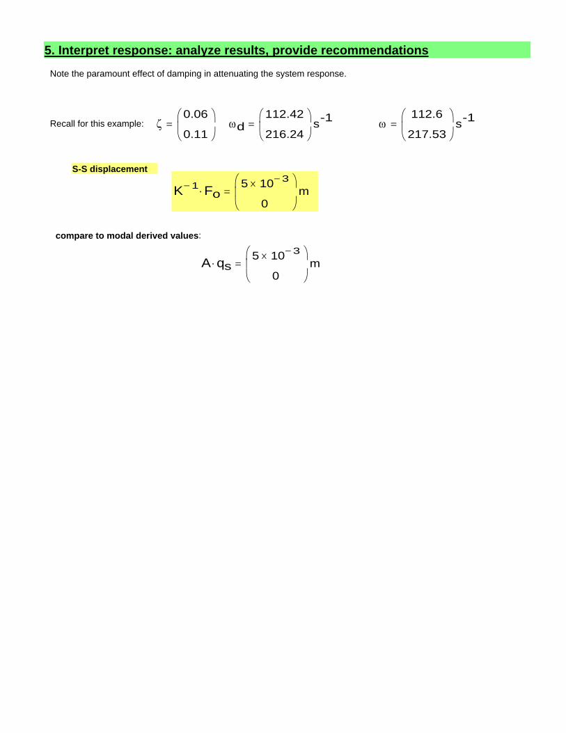
5. Interpret response: analyze results, provide recommendations
Note the paramount effect of damping in attenuating the system response.
Recall for this example: ζ0.06
0.11⎛⎜⎝
⎞⎟⎠
= ωd112.42
216.24⎛⎜⎝
⎞⎟⎠s-1= ω
112.6
217.53⎛⎜⎝
⎞⎟⎠s-1=
S-S displacement
K 1− Fo⋅5 10 3−×
0
⎛⎜⎝
⎞⎟⎠m=
compare to modal derived values:
A qs⋅5 10 3−×
0
⎛⎜⎝
⎞⎟⎠m=

Note M and K are symmetric matrices with a RIGID BODY MODE
example α 0.01s
⋅:= β .001 s⋅:=D α M⋅ β K⋅+:=
D1 103×
1− 103×
1− 103×
1 103×
⎛⎜⎝
⎞⎟⎠N
sm
⋅=
Xo0
0⎛⎜⎝
⎞⎟⎠
m⋅:= Vo0.0
0⎛⎜⎝
⎞⎟⎠
msec
⋅:=initial conditions
Applied force vector: Fo1000
980−⎛⎜⎝
⎞⎟⎠
N⋅:=
l i
STEP FORCED RESPONSE of 2-DOF mechanical system with proportional damping
ORIGIN 1:=
Dr. Luis San Andres (c) MEEN 363, 617 February 2008
The equations of motion are: (1)M2t
Xdd
2⋅ D
tXd
d⋅+ K X⋅+ Fo=
where M,D, K are matrices of inertia, damping and stiffness coefficients; and X, V=dX/dt,
d2X/dt2 are the vectors of physical displacement, velocity and acceleration, respectively. The FORCED undamped response to the initial conditions, at t=0, Xo,Vo=dX/dt, follows:
For proportional damping, D = α M + β K, so the undamped mode analysis can be used. α & β are physical constants usually determined from measurements of modal damping.
============================================================================================
The equations of motion are:
M11
M21
M12
M22
⎛⎜⎝
⎞⎟⎠ 2t
x1
x2
⎛⎜⎝
⎞⎟⎠
dd
2⋅
D11
D21
D12
D22
⎛⎜⎝
⎞⎟⎠ t
x1
x2
⎛⎜⎝
⎞⎟⎠
dd⋅+
K11
K21
K12
K22
⎛⎜⎝
⎞⎟⎠
x1
x2
⎛⎜⎝
⎞⎟⎠
⋅+F1o
F2o
⎛⎜⎝
⎞⎟⎠
= (2)
1. Set elements of inertia, stiffness & damping matricesDATA FOR problem
M100
0
0
50⎛⎜⎝
⎞⎟⎠
kg⋅:= K1 106⋅
1− 106⋅
1− 106⋅
1 106⋅
⎛⎜⎝
⎞⎟⎠
Nm
⋅:=n 2:= # of DOF

j 1 n..:=ω j λ j( ) .5:= ω
0
173.21⎛⎜⎝
⎞⎟⎠
radsec
= (4)f
ω
2 π⋅:=
f0
27.57⎛⎜⎝
⎞⎟⎠Hz=
Note that: Δ ω1( ) Δ ω2( )= 0=
For each eigenvalue, the eigenvectors (natural modes) are
j 1 n..:=Set arbitrarily first element of vector = 1
aj
1
K1 1, M1 1, λ j⋅−
K1 2, M1 2, λ j⋅−( )−
⎡⎢⎢⎢⎣
⎤⎥⎥⎥⎦
:=
a11
1⎛⎜⎝
⎞⎟⎠
= a21
2−⎛⎜⎝
⎞⎟⎠
= (5)MODAL matrix A j⟨ ⟩ aj:=
A is the matrix of eigenvectors (undampedmodal matrix): each column corresponds to an eigenvector
A1
1
1
2−⎛⎜⎝
⎞⎟⎠
=
analysis
2. Find eigenvalues (undamped natural frequencies) and eigenvectors
Set determinant of system of eqns = 0
Δ K11 M11 ω2⋅−( ) K22 M22 ω2⋅−( )⋅ K12 M12 ω2⋅−( ) K21 M21 ω2⋅−( )⋅−⎡⎣ ⎤⎦= 0= (2a)
(2b)Δ a ω4⋅ b ω2⋅+ c+= a λ2⋅ b λ⋅+ c+( )= 0= with λ ω2=
where thecoefficientsare:
a M1 1, M2 2,⋅ M1 2, M2 1,⋅−:=(2c)b K1 2, M2 1,⋅ K1 1, M2 2,⋅− K2 2, M1 1,⋅− K2 1, M1 2,⋅+:=
c K1 1, K2 2,⋅ K1 2, K2 1,⋅−:=
The roots of equation (2b) are:
(3)λ1b− b2 4 a⋅ c⋅−( ) .5−⎡⎣ ⎤⎦
2 a⋅:= λ2
b− b2 4 a⋅ c⋅−( ) .5+⎡⎣ ⎤⎦2 a⋅
:=
also known as eigenvalues. The natural frequencies follow as:
or better Dm α Mm⋅ β Km⋅+:=
Dm0
0
0
9 103×
⎛⎜⎝
⎞⎟⎠s
Nm
=Dm AT D⋅ A⋅:=
ω0
173.21⎛⎜⎝
⎞⎟⎠s-1=
Km0
0
0
9 106×
⎛⎜⎝
⎞⎟⎠
Nm
=Km AT K⋅ A⋅:=
Mm150
0
0
300⎛⎜⎝
⎞⎟⎠kg=Mm AT M⋅ A⋅:=
The natural modes satisfy the orthogonality properties
(9)so Mm1− AT M⋅ Vo⋅( )⋅=qo Mm
1− AT M⋅ Xo⋅( )⋅=
and initial conditions (modal displacement=q and modal velocity dq/dt=s)
Qm AT Fo⋅=with modal force vector: (8)
Mm 2tqd
d
2⋅ Dm
tqd
d⋅+ Km q⋅+ Qm= (7)
EOMs (1) become uncoupled in modal space:
X A q⋅=Using transformation: (6)
3. Modal transformation of physical equations to (natural) modal coordinates
2
0
2
mode 1mode 2
DOF
Aj 1,
Aj 2,
j
Plot the mode shapes:

: static displacement in modal spaceqsj
Qmj
Kmj j,
:=j 2:=
elastic mode - UNDERDAMPED
q1 t( ) qo1
so1
t⋅+Qm
1
Mm1 1,
t2
2⋅+:=
rigid body mode - NO DAMPING
4.c Build Modal responses:
Qm20
2.96 103×
⎛⎜⎝
⎞⎟⎠N=
Qm AT Fo⋅:=
4.b Find Modal forces:
so0
0⎛⎜⎝
⎞⎟⎠m s-1=qo
0
0⎛⎜⎝
⎞⎟⎠m=
so Ainv Vo⋅:=qo Ainv Xo⋅:=
Ainv Mm1− AT M⋅( )⋅:=Set inverse of modal mass matrix
4.a Find initial conditions in modal coordinates (displacement = q, velocity = s)
4. Find Modal and Physical Response for given initial condition and Constant Force vector
=========================================================================================
ωd0
172.55⎛⎜⎝
⎞⎟⎠s-1=UNDERDAMPED CASE ω
0
173.21⎛⎜⎝
⎞⎟⎠s-1=
ζ0
0.09⎛⎜⎝
⎞⎟⎠
= ONE RIGID BODY mode with null modal damping
(11)ωdkωk 1 ζk( )2−⎡⎣ ⎤⎦
.5⋅:=ζk
Dmk k,
2 Mmk k,
⋅ ωk⋅:=
k 1 n..:=Define the modal damping ratios and damped natural freqs:
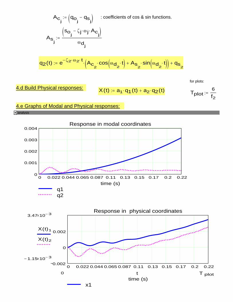
Acj
qoj
qsj
−( ):= : coefficients of cos & sin functions.
Asj
soj
ζ j ω j⋅ Acj
⋅−( )ωdj
:=
q2 t( ) e ζ2− ω2⋅ t⋅ Ac2
cos ωd2
t⋅( )⋅ As2
sin ωd2
t⋅( )⋅+( )⋅ qs2
+:=
for plots:
4.d Build Physical responses: X t( ) a1 q1 t( )⋅ a2 q2 t( )⋅+:= Tplot6f2
:=
4.e Graphs of Modal and Physical responses:analysis
0 0.022 0.044 0.065 0.087 0.11 0.13 0.15 0.17 0.2 0.220
0.001
0.002
0.003
0.004
q1q2
Response in modal coordinates
time (s)
0 0.022 0.044 0.065 0.087 0.11 0.13 0.15 0.17 0.2 0.220.002
0
0.002
x1
Response in physical coordinates
time (s)
3.47 10 3−×
1.15− 10 3−×
X t( )1
X t( )2
T plot0 t

x2
5. Interpret response: analyze results, provide recommendations
Note the paramount effect of damping in attenuating the system response.
Recall for this example: ζ0
0.09⎛⎜⎝
⎞⎟⎠
= ωd0
172.55⎛⎜⎝
⎞⎟⎠s-1= ω
0
173.21⎛⎜⎝
⎞⎟⎠s-1=
i.e., Modal damping ratios of 9% for elastic mode.