evaluation of damping estimates in the presence of closely ... · evaluation of damping estimates...
TRANSCRIPT

General rights Copyright and moral rights for the publications made accessible in the public portal are retained by the authors and/or other copyright owners and it is a condition of accessing publications that users recognise and abide by the legal requirements associated with these rights.
Users may download and print one copy of any publication from the public portal for the purpose of private study or research.
You may not further distribute the material or use it for any profit-making activity or commercial gain
You may freely distribute the URL identifying the publication in the public portal If you believe that this document breaches copyright please contact us providing details, and we will remove access to the work immediately and investigate your claim.
Downloaded from orbit.dtu.dk on: Dec 28, 2019
Evaluation of damping estimates in the presence of closely spaced modes usingoperational modal analysis techniques
Bajric, Anela; Brincker, Rune; Thöns, Sebastian
Published in:Proceedings of the 6th International Operational Modal Analysis Conference
Publication date:2015
Link back to DTU Orbit
Citation (APA):Bajric, A., Brincker, R., & Thöns, S. (2015). Evaluation of damping estimates in the presence of closely spacedmodes using operational modal analysis techniques. In Proceedings of the 6th International Operational ModalAnalysis Conference

EVALUATION OF DAMPING ESTIMATES IN THE PRES-ENCE OF CLOSELY SPACED MODES USING OPERATIONALMODAL ANALYSIS TECHNIQUES
Anela Bajric 1, Rune Brincker 2, Sebastian Thons 3
1 PhD Student, Department of Civil Engineering, Technical University of Denmark, [email protected] Professor, Department of Engineering, Aarhus University, [email protected] Associate Professor, Department of Civil Engineering, Technical University of Denmark, [email protected].
ABSTRACTThe Operational Modal Analysis (OMA) techniques provide in most cases reasonably accurate estimates
of structural frequencies and mode shapes. They are however known to produce erroneous structural
damping estimates, which are presumably thought to be due to inherent random- or bias errors that have
varying significance for different techniques. This paper evaluates the sensitivity of damping estimates
of closely spaced modes for two existing OMA techniques derived in the time and frequency domain;
namely Eigensystem Realization Algorithm (ERA) and Frequency Domain Decomposition (FDD). The
evaluation is based on identification using random response from white noise loading of a three degree-
of-freedom (3DOF) system numerically established from specified modal parameters for a range of nat-
ural frequencies. The numerical model provides comparisons of the effectiveness of damping estimation
for a variety of damping levels, signal noise and the sensitivity to closely spaced modes. It is shown that
FDD has a tendency to overestimate damping due to leakage in the estimated spectral density function
and it is a more sensitive technique to system changes than the ERA. The accuracy of damping estimates
converges with increased frequency of the system, which is mainly a result of the problematic regions in
the correlation function estimation. These regions cause amplification of the damping estimation errors
at higher levels of damping. This emphasizes the importance of correctly estimating the correlation func-
tion and spectral density as bias will potentially result in large errors in the estimation of highly damped
systems. It is concluded that damping estimated are sensitive to closely spaced modes. In addition, it is
found that two closely spaced modes will also disturb the estimation of damping of the remaining modes
in the system.
Keywords: Operational Modal Analysis, structural damping, Eigensystem Realization Algorithm, Fre-quency Domain Decomposition, closely spaced modes.

1. INTRODUCTION
The Operational Modal Analysis (OMA) techniques provide reasonably accurate estimates of struc-
tural frequencies and mode shapes. In contrast though, they are known to produce erroneous structural
damping estimates due to bias and random errors, reducing the reliability of structural design for dy-
namic effects. Potential factors influencing the estimation of damping include test procedure and quality
of measurements. Additionally, significant dispersion of random and bias error of damping estimates
for various mechanisms has been reported using available OMA techniques. Inconsistent estimates of
aerodynamic damping from full-scale monitoring of the bridge cables on the Oresund Brige, using the
Eigensystem Realization Algorithm (ERA)[2] and the Stochastic Subspace Identification (SSI) [3], was
reported in 2011 by Georgakis et al. [1], . Similarly, dispersion of lateral damping estimates was iden-
tified using the Enhanced Frequency Domain Decomposition (EFDD) [4] and SSI for 10 instrumented
bridges in California from ground motion data, Ortiz et al. [5]. Sensistivity studies of damping estimates
have also been studied to render the effects of crack development on energy dissipation using SSI and
Random Decrement (RD) [6] for the application of identifying structural damage through changes in
damping, Gutenbrunner et al. [7]. Further examples on the quality of the damping estimates using OMA
techniques can be found in [8], [9], [10].
The clear distinction between OMA techniques is the domain of implementation. The covariance-drive
or data-driven techniques are referred to as time domain techniques, and the methods based on the spec-
tral density function are referred to as frequency domain techniques. In this paper a time domain and a
frequency domain technique are compared, the ERA and FDD respectively. These were demonstrated
as two effective techniques from a numerical study of the reliability and accuracy of damping estimates
comparing selected OMA techniques, Bajric et al. [11], [12].
This paper focuses on the quality of damping estimates in the presence of closely spaced modes and
addresses the challenge in estimating damping in the transition region between moderately- and closely
spaced modes. The evaluation of the techniques as damping estimators is based on the performance of
a numerically established three degree-of-freedom (3DOF) system. The systems’ response is random,
with varying levels of signal noise, and varying levels of damping. Parameter values are chosen to be
representative of those associated with large civil engineering structures.Closely spaced modes are often
encountered for very flexible structures, characterized by low natural frequencies and damping ratios.
The proximity of natural frequencies reduces the quality of the mode shapes [13],[14], however it is
unknown how this is reflected in the estimation of damping.
2. IDENTIFICATION ALGORITHMS
The two existing techniques implemented are based on identification of modal parameters in the time-
and frequency domain using the OMA toolbox [15].
2.1. Eigensystem Realization Algorithm
The idea of ERA, is to interpret the auto-correlation functions (CF) of the structural response as free
decays. The ERA technique is formulated as in the original version by Juang and Pappa [2]. The first
step is to place the free decays in two Hankel matrices. The observability and controllability matrices
are then estimated preforming a singular value decomposition (SVD) of the Hankel matrix, and from
these the discrete time system matrix is estimated. The modal parameters are estimated by performing
an eigenvalue decomposition of the estimated discrete time system matrix.
2.2. Frequency Domain Decomposition
The frequency domain identification techniques make use of the ability to estimate modal parameters
from the spectral density function (SD). In the classical frequency domain approach the natural fre-
quency is estimated from the location of the peak in the power spectral density (PSD) matrix, where the
mode shapes correspond to the rows or columns in the PSD matrix and the damping is proportional to

the width of the peaks, Bendat and Piersol [16]. The accuracy of the classical frequency domain method
breaks down in the occurrence of closely spaced modes. The FDD, introduced Brincker et al. [17], per-
mits identification of modal parameters in the presence of closely spaced modes. The method is based
on the decomposition of the spectral matrix into auto-spectral density functions. The decomposition is
performed by taking the SVD of the SD matrix at each frequency. The maximum singular values are
directly related to the natural frequencies squared and the corresponding singular vectors are related to
to the mode shapes.
Typically in the FDD the natural frequency and damping are estimated by using the information around
the peak of the SD for the SDOF system, and transforming it back to time domain by inverse Fast Fourier
Transformation (FFT) to obtain the auto correlation function [18]. This provides an opportunity to esti-
mate the natural frequencies and damping from the zero crossing times and the logarithmic decrement of
the CF for a SDOF systems. The damping in this paper, is estimated using the CF of the SDOF system,
obtained from an FDD, as an input to the Single-Input-Multiple-Output (SIMO) version of the Ibrahim
Time Domain (ITD) technique, Ibrahim [19].
2.3. Identifying and separating close modes
In the case of repeated natural frequencies, the properties of two modes become one shared property
and hence a challenge to firstly identify and then separate two closely spaced modes. Mode paring can
be preformed based on the estimated natural frequency, the estimated damping or the mode shape. For
the later the estimate can be evaluated through the widely used Modal Assurance Criterion (MAC). The
MAC value indicates the degree of coherence between an identified mode and the ideal counterpart from
an i.e. FE model, Allemang and Brown 1982 [20]. It has however been found that the mode shapes are
highly sensitive when the frequency difference of two modes tend to zero and the MAC value is in that
case not a meaningful measure. The subspace spanned by the two mode shapes is stable in comparison
to the sensitive mode shapes, and has emerged as the preferred method for mode paring, [14],[21]. It is
not only damping estimates that are inaccurate using OMA techniques, but also modeling of damping
is at this stage not developed to reveal accurate characteristics of the energy dissipation and it becomes
challenging to compare the estimated and modeled damping. In this paper mode paring of closely spaced
modes is solemnly based on mode paring according to the predefined frequency of the numerical system.
3. NUMMERICAL SIMMULATIONS AND RESULTS
A schematic illustration of the main numerical procedure is illustrated in Figure 1. The steps are as
follows; specification of parameters of the system, computation of the random response to white noise
loading, signal processing to estimate the CF and SD estimates as input for the two system identificationtechniques, ERA and FDD, modal parameter extraction and finally a statistical analysis of the damping
estimates. The identification was automated and repeated 100 times for varying levels of damping ra-
tios, separated and closely spaced modes and signal noise levels, which led to eight tested configurations
listed in Table 3. Details of the main steps in the numerical procedure are described in the following.
The system is a 3DOF system with specified natural frequencies fa,i, random normal mode shapes φa,i
and the equivalent level of damping, ζa,i, for all three modes, where the index a refers to the assigned
value and i refers to the mode number. The damping is presented as a percentage of the critical damp-
ing. The first- and third natural frequency of the system were constant, with the values fa,1=1Hz and
fa,3=3Hz, and the second was varied through a range, such that fa,2=[0.5:3.5]Hz. For the sake of sim-
plicity the second mode will be refereed to as the second mode.
The response of the system to random excitation is computed using FFT of the Frequency Response
Function (FRF) of a 1DOF system. Random excitation was simulated as white noise and the signal noise
level was simulated as white noise with unit variance based on the root mean square (RMS). The limited
time series length and frequency resolution is known to give rise to identification problems in OMA.
Therefore a criterion was set to ensure reasonable estimates of the CF and SD, such that the estimated
damping includes minimal influence from bias. The optimal time series length is thus inversely propor-

tional to the structural damping ratio times the minimum natural frequency of interest [18]. The time
step dt was set to 0.05 sec and was held constant throughout all simulations, and the total number of data
points in the time series was adjusted according to the mentioned criterion.
The input for the ERA technique was the direct unbiased estimate of the CF from the response matrix,
Persol and Bendat [16]. The length of the time lag vector denoted τ , is equal to the number of data points
in the time series. For each CF the first cycle was neglected to avoid the influence of signal noise. The
portion of the CF characterized by a large amplitude was selected, which results in removal of the tail.
The truncation point was at an amplitude of 20% of the maximum amplitude.
Figure 1: Schematic illustration of the numerical procedure. The systems natural frequencies, fa,i, mode shapes
φa,i and damping ratios ζa,i are specified. The system identification is preformed with the Eigensystem Realization
Algorithm (ERA) and two versions of the Frequency Domain Decomposition (FDD). FDD 1 is the original version.
FDD 2 excludes specific regions in the correlation function. The estimated parameters are the damping ratios,
ζ1i , ..., ζNi for the i-th mode and N repeated simulations.
For identification using FDD the input was the half spectral density function, which was computed using
zero padded direct CF estimates and transformed back to the time domain using Inverse FFT (IFFT).
Before preforming the IFFT a flat-triangular window was multiplied with the CF to suppress side lobe
noise. The side lobe noise is always present due to the noise tail on the CF, which prevents the CF from
decaying to zero inside the considered time interval.In the boundaries of the time interval, when the
window approaches zero, the application of a triangular window amplifies the noise tail. Therefore two
versions of the FDD identification are carried out. The first, referred to as FDD 1, applies the full CF
as input for the ITD, as described in section 2.2. The second version, referred to as FDD 2, applies the
innermost part of the adjusted CF as described above for the ERA input. It should be noted that in the
FDD the user decides where the natural frequency is placed. In these simulations the assigned natural
frequencies of the system was used in the decision making of the peak in the SVD plot.
Mode paring was preformed with a simplified algorithm, which sorts the modes according to the prior
knowledge of the natural frequency. In these simulations the level of damping is equal on all modes, and
in the presence of identical frequencies for two modes the assigned mode was not considered to be of
high significance.
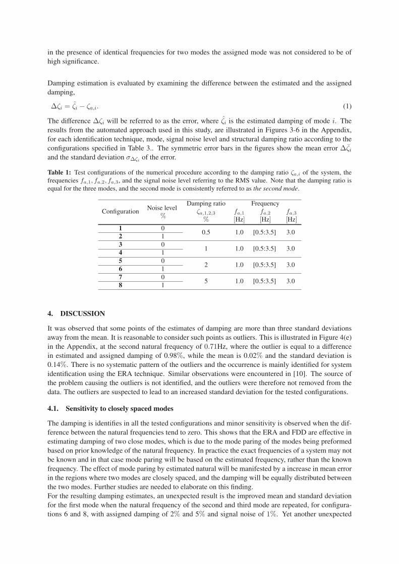
Damping estimation is evaluated by examining the difference between the estimated and the assigned
damping,
Δζi = ζi − ζa,i. (1)
The difference Δζi will be referred to as the error, where ζi is the estimated damping of mode i. The
results from the automated approach used in this study, are illustrated in Figures 3-6 in the Appendix,
for each identification technique, mode, signal noise level and structural damping ratio according to the
configurations specified in Table 3.. The symmetric error bars in the figures show the mean error Δζiand the standard deviation σΔζi of the error.
Table 1: Test configurations of the numerical procedure according to the damping ratio ζa,i of the system, the
frequencies fa,1, fa,2, fa,3, and the signal noise level referring to the RMS value. Note that the damping ratio is
equal for the three modes, and the second mode is consistently referred to as the second mode.
ConfigurationNoise level
%
Damping ratio Frequency
ζa,1,2,3 fa,1 fa,2 fa,3% [Hz] [Hz] [Hz]
1 00.5 1.0 [0.5:3.5] 3.02 1
3 01 1.0 [0.5:3.5] 3.04 1
5 02 1.0 [0.5:3.5] 3.06 1
7 05 1.0 [0.5:3.5] 3.08 1
4. DISCUSSION
It was observed that some points of the estimates of damping are more than three standard deviations
away from the mean. It is reasonable to consider such points as outliers. This is illustrated in Figure 4(e)
in the Appendix, at the second natural frequency of 0.71Hz, where the outlier is equal to a difference
in estimated and assigned damping of 0.98%, while the mean is 0.02% and the standard deviation is
0.14%. There is no systematic pattern of the outliers and the occurrence is mainly identified for system
identification using the ERA technique. Similar observations were encountered in [10]. The source of
the problem causing the outliers is not identified, and the outliers were therefore not removed from the
data. The outliers are suspected to lead to an increased standard deviation for the tested configurations.
4.1. Sensitivity to closely spaced modes
The damping is identifies in all the tested configurations and minor sensitivity is observed when the dif-
ference between the natural frequencies tend to zero. This shows that the ERA and FDD are effective in
estimating damping of two close modes, which is due to the mode paring of the modes being preformed
based on prior knowledge of the natural frequency. In practice the exact frequencies of a system may not
be known and in that case mode paring will be based on the estimated frequency, rather than the known
frequency. The effect of mode paring by estimated natural will be manifested by a increase in mean error
in the regions where two modes are closely spaced, and the damping will be equally distributed between
the two modes. Further studies are needed to elaborate on this finding.
For the resulting damping estimates, an unexpected result is the improved mean and standard deviation
for the first mode when the natural frequency of the second and third mode are repeated, for configura-
tions 6 and 8, with assigned damping of 2% and 5% and signal noise of 1%. Yet another unexpected

result is the increased mean and standard deviation for the third mode, in particular for FDD 1 and FDD
2, when the first and second natural frequency is repeated. In conclusion, closely spaced modes will not
only affect the modes with closely spaced natural frequencies but the damping estimates of the whole
system.
4.2. Comparison of estimation techniques
Figures 3-6 in the Appendix, show a significant decrease in mean and standard deviation of the damping
estimation error using the correlation-driven realizations with the ERA techniques compared to the FDD
1 and FDD 2. The identification procedure consists of steps, and it is the authors’ understanding that the
main estimation errors are introduced in the step denoted signal processing. This step contains estimation
of the CF and estimation of the SD. The estimation of the CF is mainly dependent of the time lag. There
are however several errors introduced in the estimation of the SD: 1) the bias error caused by frequency
resolution and the length of the time series, 2) the variance error caused by averaging the SD, and 3)
aliasing associated with sampling. The assessment of the damping estimation errors will in the following
be attributed to the above mentioned estimation errors.
4.3. Overestimation of damping in the frequency domain
The most dominant difference between the domains of identification is the overestimation of damping in
the frequency domain, which can lead to unrealistically larger damping ratio estimates. This condition
is related to the power of the signal ’leaking’ out to neighboring frequencies, well known as spectral
leakage [22]. This phenomenon occurs due to FFT’s assumed periodicity within the finite measurement
time with N samples of the signal. The modal peaks of the SD functions will become wider as a result
of leakage. Each modal peak is proportional to the damping, hence damping will be overestimated. This
effect is emphasized in estimation of damping using methods outside of OMA, which are also dependent
on the SD [23],[24]. In principle an unbiased estimate of modal parameters in the frequency domain can
only be obtained by means of infinite records. The length of the record is crucial for reliable damping
estimates. Overestimation of damping in the frequency domain cannot be regarded as a consistent final
conclusion. In a special case with a high level of damping, see Figure 6(f) in the Appendix, damping will
be underestimated for higher modes and further amplification of underestimation occurs in the presence
of signal noise. The attributes to this result are discussed in section 4.6.
4.4. Problematic regions in the correlation function.
An additional dominant difference between the techniques is the decrease in mean and standard deviation
between the results obtained with the FDD 1 and FDD 2 techniques. The observed decrease in the
estimation error when using the FDD2, is an effect of excluding the problematic regions of the CF.
Namely the first cycle and the so called noise tail. When the noise tail is included the decay of the CF at
higher time lags will tend to represent the correlation of the signal noise, rather than the physical system,
and the decay will never reach zero. A careful selection of the CF is therefore essential.
4.5. Convergence of damping estimates for higher modes
A common characteristic for the techniques is the converging error of mean and standard deviation of
damping estimation for increased frequencies of the system. The trend is clear for identification of
damping for the second mode with natural frequencies ranging from 0.5Hz to 3.5Hz, Figures 3-6 (c) and
(d) in the Appendix. This convergence of error is mainly due to the inadequate amount of information of
the decaying CF at lower frequencies of the system. It is observed that the convergence rate of the error
is dependent on the time step. Figure 2 shows the estimation errors of the second mode with variable
sampling resolutions and constant time window. The convergence rate of the standard deviation is in
particular dependent on the time step for higher modes. For these modes the sampled data does not
recognize the frequency component adequately if the time step is too large. The accuracy of damping for
the lower modes will not decrease when the time step is adjusted, simply because the error is due to the
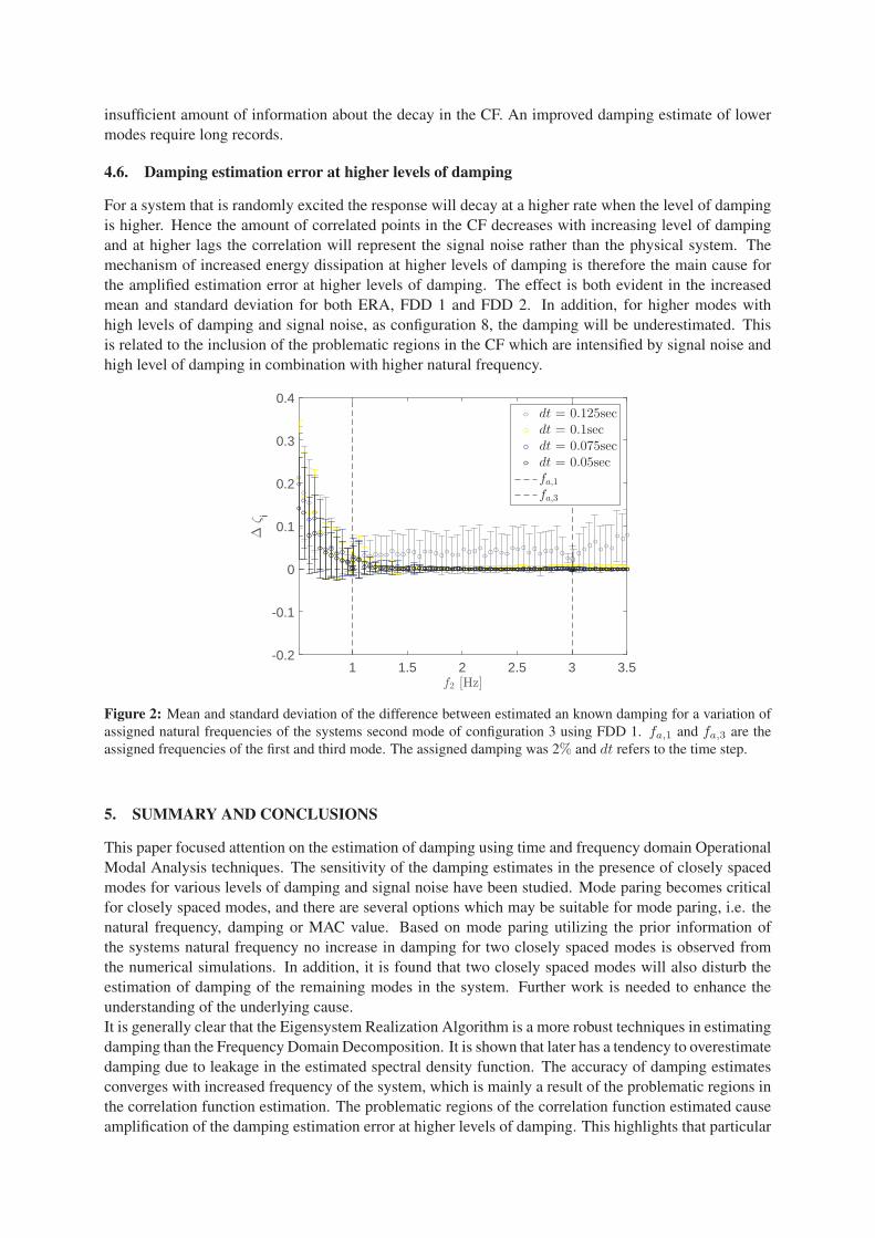
insufficient amount of information about the decay in the CF. An improved damping estimate of lower
modes require long records.
4.6. Damping estimation error at higher levels of damping
For a system that is randomly excited the response will decay at a higher rate when the level of damping
is higher. Hence the amount of correlated points in the CF decreases with increasing level of damping
and at higher lags the correlation will represent the signal noise rather than the physical system. The
mechanism of increased energy dissipation at higher levels of damping is therefore the main cause for
the amplified estimation error at higher levels of damping. The effect is both evident in the increased
mean and standard deviation for both ERA, FDD 1 and FDD 2. In addition, for higher modes with
high levels of damping and signal noise, as configuration 8, the damping will be underestimated. This
is related to the inclusion of the problematic regions in the CF which are intensified by signal noise and
high level of damping in combination with higher natural frequency.
f2 [Hz]1 1.5 2 2.5 3 3.5
Δζ
i
-0.2
-0.1
0
0.1
0.2
0.3
0.4dt = 0.125secdt = 0.1secdt = 0.075secdt = 0.05secfa,1
fa,3
Figure 2: Mean and standard deviation of the difference between estimated an known damping for a variation of
assigned natural frequencies of the systems second mode of configuration 3 using FDD 1. fa,1 and fa,3 are the
assigned frequencies of the first and third mode. The assigned damping was 2% and dt refers to the time step.
5. SUMMARY AND CONCLUSIONS
This paper focused attention on the estimation of damping using time and frequency domain Operational
Modal Analysis techniques. The sensitivity of the damping estimates in the presence of closely spaced
modes for various levels of damping and signal noise have been studied. Mode paring becomes critical
for closely spaced modes, and there are several options which may be suitable for mode paring, i.e. the
natural frequency, damping or MAC value. Based on mode paring utilizing the prior information of
the systems natural frequency no increase in damping for two closely spaced modes is observed from
the numerical simulations. In addition, it is found that two closely spaced modes will also disturb the
estimation of damping of the remaining modes in the system. Further work is needed to enhance the
understanding of the underlying cause.
It is generally clear that the Eigensystem Realization Algorithm is a more robust techniques in estimating
damping than the Frequency Domain Decomposition. It is shown that later has a tendency to overestimate
damping due to leakage in the estimated spectral density function. The accuracy of damping estimates
converges with increased frequency of the system, which is mainly a result of the problematic regions in
the correlation function estimation. The problematic regions of the correlation function estimated cause
amplification of the damping estimation error at higher levels of damping. This highlights that particular
attention is needed in estimating the correlation function and spectral density as the introduced bias will
potentially result in large errors in the estimation of highly damped systems.
It is important to note that the evaluation of damping estimates was limited to a linear time-invariant
system with normal modes, proportional damping of equal level on all modes and white noise excitation.
Due to the non-proportional nature of damping and the possible presence of non-linearities, the modal
damping ratio identification should be examined in future for complex modes. Excitation of real struc-
tures differ from white noise loading and can potentially lead to further scattering in the estimation of
damping.
REFERENCES
[1] Georgakis, C.T. and Acampora, A. (2011) Determination of the aerodynamic damping of dry and
wet bridge cables from full-scale monitoring. In: Proc. 9th Int. Symposium on Cable Dynamics(pp. 242-250). Shanghai, China.
[2] Juang, J.N. and Pappa, R.S. (1985) An eigen system realization algorithm for modal parameter
identification and modal reduction. Journal of Guidance, Control, and Dynamics, 8(5), 620-627.
[3] Overschee, P.V. and De Moor, B. (1996) Subspace Identification for Linear Systems. Kluwer
Academic Publishers.
[4] Brincker, R.,Ventura, C. and Andersen, P. (2001) Damping estimation by frequency domain de-
composition. In: Proc. 19th Int. Modal Analysis Conference (pp. 101-110). Kissimmee, Florida,
USA.
[5] Ortiz, A.R.,Ventura, C. and Catacoli, S.S. (2013) Sensitivity Analysis of the Lateral Damping of
Bridges for Low Levels of Vibration. In: Proc. 131st Int. Modal Analysis Conference (pp. 101-110).
San Antonio, Texas, USA.
[6] Cole, H. (1973) On-Line Failure Detection and Damping Measurement of Aerospace Structures byRandom Decrement Signatures . NASA CR-2205.
[7] Guttenbrunner, G.,Savov, K. and Wenzel, H. (2007) Sensitivity studies on damping estimation. In:
Proc. 2nd Int. Conference on Experimental Vibration Analysis for Civil Engineering Structures.
Porto, Portugal.
[8] Tamura, Y.,Yoshida, A.,Zhang L.,Ito, T.,Nakata, S. and Sato, K. (2005) Examples of modal identi-
fication of structures in Japan by FDD and MRD techniques. In: Proc. 1st Int. Operational ModalAnalysis Conference. Copenhagen, Denmark.
[9] Magalhes, F.,Cunha, A,Caetano, E. and Brincker, R. (2010) Damping estimation using free decays
and ambient vibration tests. Journal of Mechanical Systems and Signal Processing, 24 (5), 1274-
1290.
[10] Pridham, B.A. and Wilson, J.C. (2003) A study on errors in correlation-driven stochastic realization
using short data sets. Probabilistic Engineering Mechanics 18(1), 61-77.
[11] Bajric, A.,Brincker, R. and Georgakis, C.T. (2014) Evaluation of damping using time domain
Operational Modal Analysis techniques. In: Prestented at, 2014 Society of Experimental MechanicsConference and International Symposium on Intensive Loading and its Effects. Beijing, China.
[12] Bajric, A.,Georgakis, C.T. and Brincker, R. (2015) Evaluation of damping using frequency domain
Operational Modal Analysis techniques. In: Proc. 33rd Int. Modal Analysis Conference. Orlando,
Florida, USA.
[13] Malekjafarian, A.,Brincker, R.,Ashory, M.R., and Khitibi, M.M. (2010) Identification of closely
spaced modes using Ibrahim Time Domain method. In: Proc. 4th Int. Operational Modal AnalysisConference. Istanbul, Turkey.
[14] Brincker, R. (2015) Mode shape sensitivity of two closely spaced eigenvalues. Journal of Soundand Vibration 334, 377-387.
[15] Brincker, R.,Ventura, C. (2015) Introduction to Operational Modal Analysis. Wiley.
[16] Bendat, J.S. and Piersol, A.G. (1993) Engineering applications of correlation and spectral analysis.
2nd edition, John Wiley & Sons.
[17] Brincker, R.,Zhang, L. and Andersen, P. (2000) Modal identification from ambient responses using
frequency domain decomposition. In: Proc. 18th Int. Modal Analysis Conference (pp. 625-630).
San Antonio, Texas, USA.
[18] Brincker, R. (2014) Some Elements of Operational Modal Analysis. Journal of Shock and Vibra-tion, 2014.
[19] Ibrahim, S.R. and Milkulcik, E.C. (1977) A method for direct identification of vibration parameters
from the free response. The Shock and Vibration Bulletin, 47, 183-196.
[20] Allemang, R.J. and Brown, D.L. (1982) A correlation coefficient for modal vector analysis. In:
Proc. 1st Int. Modal Analysis Conference. Orlando, Florida, USA.
[21] Brincker, R. (2014) A local correspondence principle for mode shapes in structural dynamics.
Journal of Mechanical Systems and Signal Processing, 45(1), 91-104.
[22] Brandt, A.(2011) Noise and vibration analysis: signal analysis and experimental procedures.. John
Wiley & Sons.
[23] Jeary, A.P. (1986) Damping in tall buildings a mechanism and a predictor.. In: Earthquakeengineering & structural dynamics 14(5), 733-750.
[24] Tamura, Y.,Zhang L.M.,Yoshida A.,Nakata, S. and Itoh, T. (2002) Ambient vibration tests and
modal identification of structures by FDD and 2DOF-RD technique. In: Proc. of the structuralengineers world congress . Yokohama, Japan.
APPENDIX
f2 [Hz]0.5 1 1.5 2 2.5 3 3.5
Δζ i
-0.2
-0.1
0
0.1
0.2
0.3
0.4FDD 1FDD 2ERAfa,1
fa,3
(a) Mode 1, ζa,1 = 0.5%, signal noise 0%.
f2 [Hz]0.5 1 1.5 2 2.5 3 3.5
Δζ i
-0.2
-0.1
0
0.1
0.2
0.3
0.4
(b) Mode 1, ζa,1 = 1%, signal noise 0%.
f2 [Hz]0.5 1 1.5 2 2.5 3 3.5
Δζ i
-0.2
-0.1
0
0.1
0.2
0.3
0.4
(c) Mode 2, ζa,2 = 0.5%, signal noise 0%.
f2 [Hz]0.5 1 1.5 2 2.5 3 3.5
Δζ i
-0.2
-0.1
0
0.1
0.2
0.3
0.4
(d) Mode 2, ζa,2 = 1%, signal noise 0%.
f2 [Hz]0.5 1 1.5 2 2.5 3 3.5
Δζ i
-0.2
-0.1
0
0.1
0.2
0.3
0.4
(e) Mode 3, ζa,3 = 0.5%, signal noise 0%.
f2 [Hz]0.5 1 1.5 2 2.5 3 3.5
Δζ i
-0.2
-0.1
0
0.1
0.2
0.3
0.4
(f) Mode 3, ζa,3 = 1%, signal noise 0%.
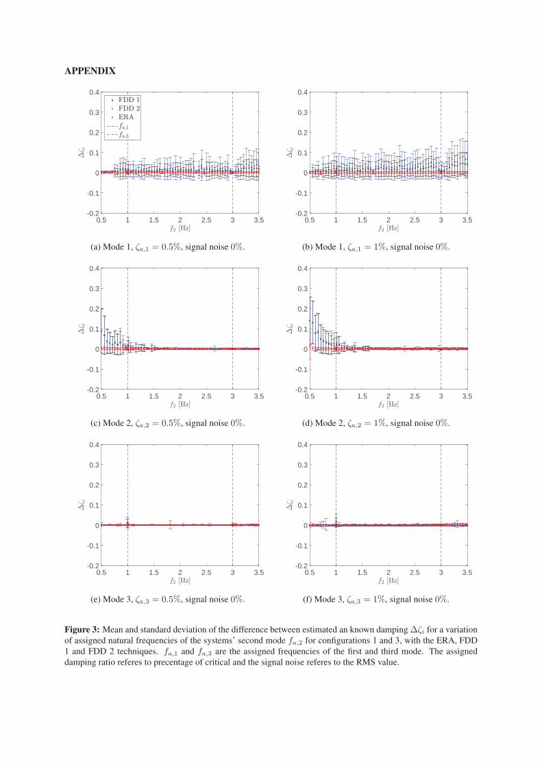
Figure 3: Mean and standard deviation of the difference between estimated an known damping Δζi for a variation
of assigned natural frequencies of the systems’ second mode fa,2 for configurations 1 and 3, with the ERA, FDD
1 and FDD 2 techniques. fa,1 and fa,3 are the assigned frequencies of the first and third mode. The assigned
damping ratio referes to precentage of critical and the signal noise referes to the RMS value.

f2 [Hz]0.5 1 1.5 2 2.5 3 3.5
Δζ i
-0.2
-0.1
0
0.1
0.2
0.3
0.4FDD 1FDD 2ERAfa,1
fa,3
(a) Mode 1, ζa,1 = 2%, signal noise 0%.
f2 [Hz]0.5 1 1.5 2 2.5 3 3.5
Δζ i
-0.2
-0.1
0
0.1
0.2
0.3
0.4
(b) Mode 1, ζa,1 = 5%, signal noise 0%.
f2 [Hz]0.5 1 1.5 2 2.5 3 3.5
Δζ i
-0.2
-0.1
0
0.1
0.2
0.3
0.4
(c) Mode 2, ζa,2 = 2%, signal noise 0%.
f2 [Hz]0.5 1 1.5 2 2.5 3 3.5
Δζ i
-0.2
-0.1
0
0.1
0.2
0.3
0.4
(d) Mode 2, ζa,2 = 5%, signal noise 0%.
f2 [Hz]0.5 1 1.5 2 2.5 3 3.5
Δζ i
-0.2
-0.1
0
0.1
0.2
0.3
0.4
(e) Mode 3, ζa,3 = 2%, signal noise 0%.
f2 [Hz]0.5 1 1.5 2 2.5 3 3.5
Δζ i
-0.2
-0.1
0
0.1
0.2
0.3
0.4
(f) Mode 3, ζa,3 = 5%, signal noise 0%.
Figure 4: Mean and standard deviation of the difference between estimated an known damping Δζi for a variation
of assigned natural frequencies of the systems’ second mode fa,2 for configurations 5 and 7, with the ERA, FDD
1 and FDD 2 techniques. fa,1 and fa,3 are the assigned frequencies of the first and third mode. The assigned
damping ratio referes to precentage of critical and the signal noise referes to the RMS value.
f2 [Hz]0.5 1 1.5 2 2.5 3 3.5
Δζ i
-0.2
-0.1
0
0.1
0.2
0.3
0.4FDD 1FDD 2ERAfa,1
fa,3
(a) Mode 1, ζa,1 = 0.5%, signal noise 1%.
f2 [Hz]0.5 1 1.5 2 2.5 3 3.5
Δζ i
-0.2
-0.1
0
0.1
0.2
0.3
0.4
(b) Mode 1, ζa,1 = 1%, signal noise 1%.
f2 [Hz]0.5 1 1.5 2 2.5 3 3.5
Δζ i
-0.2
-0.1
0
0.1
0.2
0.3
0.4
(c) Mode 2, ζa,2 = 0.5%, signal noise 1%.
f2 [Hz]0.5 1 1.5 2 2.5 3 3.5
Δζ i
-0.2
-0.1
0
0.1
0.2
0.3
0.4
(d) Mode 2, ζa,2 = 1%, signal noise 1%.
f2 [Hz]0.5 1 1.5 2 2.5 3 3.5
Δζ i
-0.2
-0.1
0
0.1
0.2
0.3
0.4
(e) Mode 3, ζa,3 = 0.5%, signal noise 1%.
f2 [Hz]0.5 1 1.5 2 2.5 3 3.5
Δζ i
-0.2
-0.1
0
0.1
0.2
0.3
0.4
(f) Mode 3, ζa,3 = 1%, signal noise 1%.
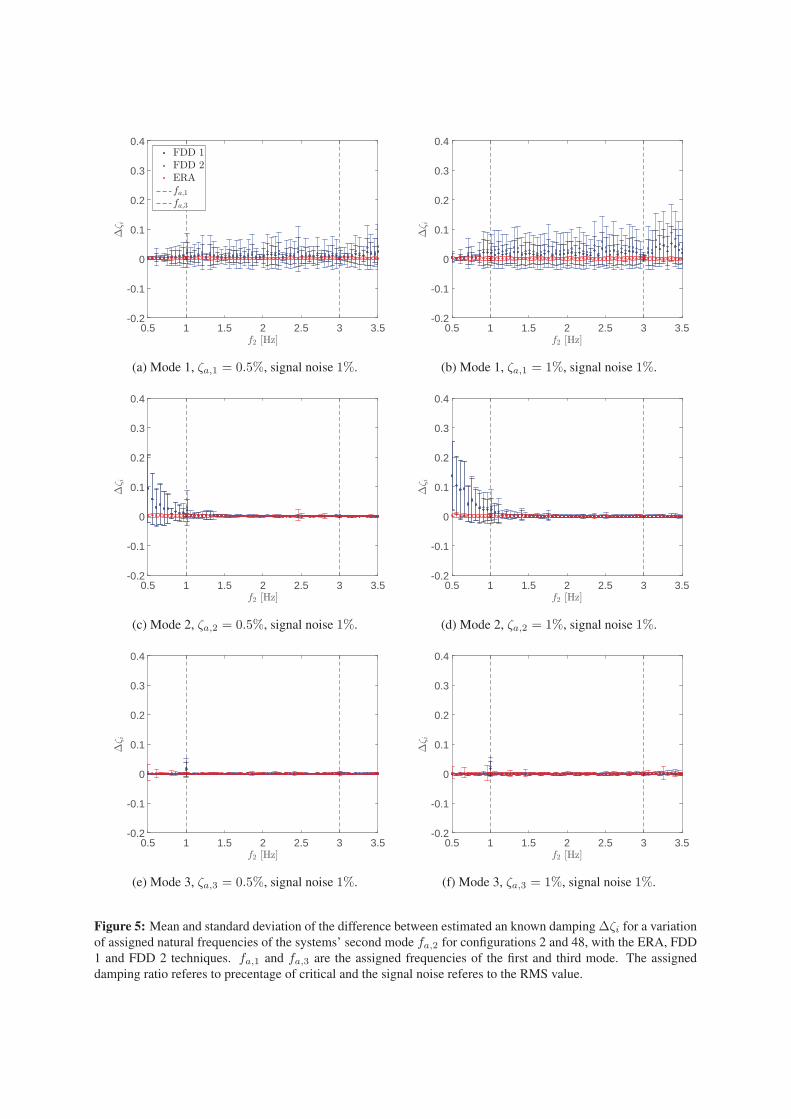
Figure 5: Mean and standard deviation of the difference between estimated an known damping Δζi for a variation
of assigned natural frequencies of the systems’ second mode fa,2 for configurations 2 and 48, with the ERA, FDD
1 and FDD 2 techniques. fa,1 and fa,3 are the assigned frequencies of the first and third mode. The assigned
damping ratio referes to precentage of critical and the signal noise referes to the RMS value.

f2 [Hz]0.5 1 1.5 2 2.5 3 3.5
Δζ i
-0.2
-0.1
0
0.1
0.2
0.3
0.4FDD 1FDD 2ERAfa,1
fa,3
(a) Mode 1, ζa,3 = 2%, signal noise 1%.
f2 [Hz]0.5 1 1.5 2 2.5 3 3.5
Δζ i
-0.2
-0.1
0
0.1
0.2
0.3
0.4
(b) Mode 1, ζa,3 = 5%, signal noise 1%.
f2 [Hz]0.5 1 1.5 2 2.5 3 3.5
Δζ i
-0.2
-0.1
0
0.1
0.2
0.3
0.4
(c) Mode 2, ζa,3 = 2%, signal noise 1% .
f2 [Hz]0.5 1 1.5 2 2.5 3 3.5
Δζ i
-0.2
-0.1
0
0.1
0.2
0.3
0.4
(d) Mode 2, ζa,3 = 5%, signal noise 1%.
f2 [Hz]0.5 1 1.5 2 2.5 3 3.5
Δζ i
-0.2
-0.1
0
0.1
0.2
0.3
0.4
(e) Mode 3, ζa,3 = 2%, signal noise 1% .
f2 [Hz]0.5 1 1.5 2 2.5 3 3.5
Δζ i
-0.2
-0.1
0
0.1
0.2
0.3
0.4
(f) Mode 3, ζa,3 = 5%, signal noise 1%.
Figure 6: Mean and standard deviation of the difference between estimated an known damping Δζi for a variation
of assigned natural frequencies of the systems’ second mode fa,2 for configurations 6 and 8, with the ERA, FDD
1 and FDD 2 techniques. fa,1 and fa,3 are the assigned frequencies of the first and third mode. The assigned
damping ratio referes to precentage of critical and the signal noise referes to the RMS value.