Ferrite (N87) core materials are an oxide made from Fe (iron), Mn (manganese), and Zn (zinc), which are commonly referred to as manganese zinc ferrites. They exhibit good magnetic properties (high permeability and saturation induction) below the Curie temperature and have a rather high electrical resistivity. These materials can be used up to very high frequencies (up to 3 MHz) without laminating, as is the normal requirement for magnetic materials to reduce eddy current losses. Because of their comparatively low losses at high frequencies, they form an essential part of inductors and transformers used in today’s main application areas of telecommunications, power conversion, and interference suppression. They are produced in a variety of shapes, including toroids, E-cores, U-cores, I-cores, and pot cores.

Date: September 2018Revision 0.1

© U.S. Department of Energy - National Energy Technology Laboratory

Fig. 2: Illustration of core dimensions

Dimensions

Table 1: Core dimensions

Description Symbol Finished dimension (mm)

Width of core A 141

Height of core B 157

Depth of core (or cast width) D 30

Thickness or build E 41

Width of core window F 50

Height of core window G 67

Gap width HMinimum

(cut surface to cut surface)

This technical effort was performed in support of the National Energy Technology Laboratory’s ongoing research in DOE’s The Offi ce of Electricity’s (OE) Transformer Resilience and Advanced Components (TRAC) program under the RES contract DE-FE0004000.

Acknowledgement

This project was funded by the Department of Energy, National Energy Technology Laboratory, an agency of the United States Government, through a support contract with AECOM. Neither the United States Government nor any agency thereof, nor any of their employees, nor AECOM, nor any of their employees, makes any warranty, expressed or implied, or assumes any legal liability or responsibility for the accuracy, completeness, or usefulness of any information, apparatus, product, or process disclosed, or represents that its use would not infringe privately owned rights. Reference herein to any specifi c commercial product, process, or service by trade name, trademark, manufacturer, or otherwise, does not necessarily constitute or imply its endorsement, recommendation, or favoring by the United States Government or any agency thereof. The views and opinions of authors expressed herein do not necessarily state or refl ect those of the United States Government or any agency thereof.

Disclaimer

Fig. 1: Core under test (Ferrite core)

MnZ

n Fe

rrite

(N87

) cor

e

MnZn Ferrite Material(EPCOS N87)datasheet

2

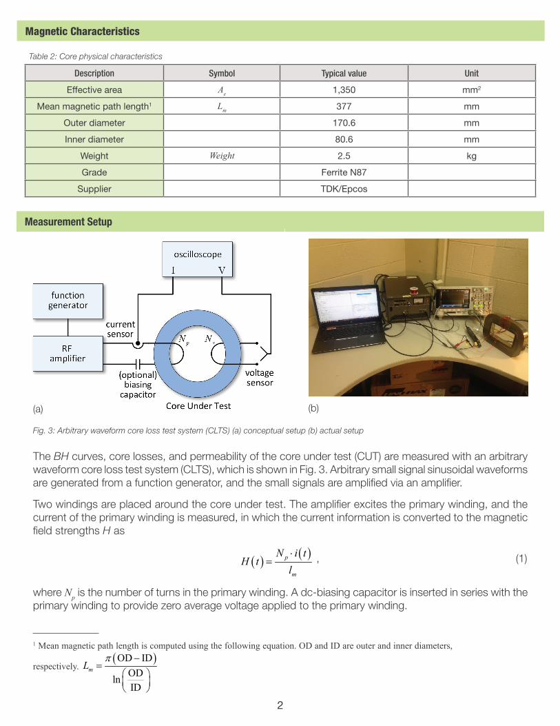
Table 2: Core physical characteristics

Description Symbol Typical value Unit

Effective area Ae 1,350 mm2

Mean magnetic path length1 Lm 377 mm

Outer diameter 170.6 mm

Inner diameter 80.6 mm

Weight Weight 2.5 kg

Grade Ferrite N87

Supplier TDK/Epcos

Measurement Setup

Fig. 3: Arbitrary waveform core loss test system (CLTS) (a) conceptual setup (b) actual setup

(a) (b)

The BH curves, core losses, and permeability of the core under test (CUT) are measured with an arbitrary waveform core loss test system (CLTS), which is shown in Fig. 3. Arbitrary small signal sinusoidal waveforms are generated from a function generator, and the small signals are amplifi ed via an amplifi er.

Two windings are placed around the core under test. The amplifi er excites the primary winding, and the current of the primary winding is measured, in which the current information is converted to the magnetic fi eld strengths H as

( ) ( )p

m

N i tH t

l⋅

= , (1)

where Np is the number of turns in the primary winding. A dc-biasing capacitor is inserted in series with the primary winding to provide zero average voltage applied to the primary winding.

Magnetic Characteristics

1 Mean magnetic path length is computed using the following equation. OD and ID are outer and inner diameters,

respectively. ( )OD ID

ODlnID

mLπ −

=

3

The secondary winding is open, and the voltage across the secondary winding is measured, in which the voltage information is integrated to derive the flux density B as

( ) ( )0

1 T

s e

B t v dN A

τ τ=⋅ ∫ , (2)

where Ns is the number of turns in the secondary winding, and T is the period of the excitation waveform.

Fig. 4 illustrates three different excitation voltage waveforms and corresponding flux density waveforms. When the excitation voltage is sinusoidal as shown in Fig. 4(a), the flux is also a sinusoidal shape. When the excitation voltage is a two-level square waveform as shown in Fig. 4(b), the flux is a sawtooth shape. The average excitation voltage is adjusted to be zero via the dc-biasing capacitor, and thus, the average flux is also zero. When the excitation voltage is a three-level square voltage as shown in Fig. 4(b), the flux is a trapezoidal shape. The duty cycle is defined as the ratio between the applied high voltage time and the period. In the sawtooth flux, the duty cycle can range from 0% to 100%. In the trapezoidal flux, the duty cycle range from 0% to 50%. At 50% duty cycles, both the sawtooth and trapezoidal waveforms become identical.

It should be noted that only limited ranges of the core loss measurements are executed due to the limitations of the amplifier, such ±75V & ±6A peak ratings and 400V/µs slew rate. The amplifier model number is HSA4014 from NF Corporation. For example, it is difficult to excite the core to high saturation level at high frequency due to limited voltage and current rating of the amplifier. Therefore, the ranges of the experimental results are limited.

Additionally, the core temperature is not closely monitored; however, the core temperature can be assumed to be near room temperature.

Fig. 4: Excitation voltage waveforms and corresponding flux density waveforms (a) Sinusoidal flux, (b) Sawtooth flux, and (c) Trapezoidal flux

4

Similarly, the anhysteretic BH curves can be computed as a function of fl ux density B using the follow formula.

( ) ( )( )

( ) ( )

0

1

( )

1

ln1

1, ,1 1

k

k k

k k k k

B

B

KBr

k k k kkr

kk k k

k

B B Hr B

Br B

r B B e

ee e

β

β γ

β γ β γ

µ

µ µ

µ α δ ε ζµ

αδ ε ζβ

−

=

−

− −

=

=−

= + + +−

= = =+ +

∑ (4)

Table 3 and Table 4 lists the anhysteretic curve coeffi cients for eqs. (3) and (4), respectively.

The core anhysteretic characteristic models in eqs. (3) and (4) are based on the following references.

Scott D. Sudhoff, “Magnetics and Magnetic Equivalent Circuits,” in Power Magnetic Devices: A Multi-Objective Design Approach, 1, Wiley-IEEE Press, 2014, pp.488-

G. M. Shane and S. D. Sudhoff, “Refi nements in Anhysteretic Characterization and Permeability Modeling,” in IEEE Transactions on Magnetics, vol. 46, no. 11, pp. 3834-3843, Nov. 2010.

The estimation of the anhysteretic characteristic is performed using a genetic optimization program, which can be found in the following websites:

https://engineering.purdue.edu/ECE/Research/Areas/PEDS/go_system_engineering_toolbox

Table 3: Anhysteretic curve coeffi cients for B as a function of H

k 1 2 3 4

mk 0.616043844651630 -0.112194382351634 0.187132470680515 0.320513717783709

hk 176.000246482166 62.8368237823821 234.277066144063 85.2674214364020

nk 1 1.14154517453573 2.19358702117813 2.40337698688833

Anhysteritic BH Curves

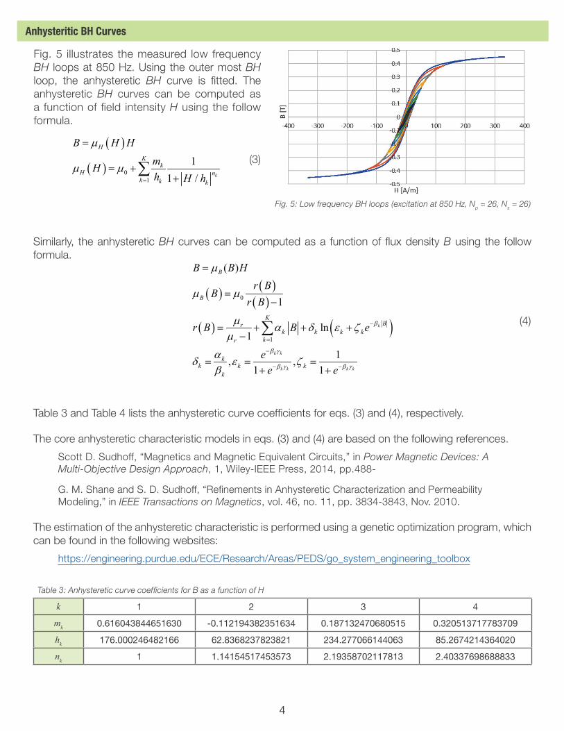
Fig. 5 illustrates the measured low frequency BH loops at 850 Hz. Using the outer most BH loop, the anhysteretic BH curve is fi tted. The anhysteretic BH curves can be computed as a function of fi eld intensity H using the follow formula.

( )

( ) 01

11 / k

H

Kk

H nk k k

B H H

mHh H h

µ

µ µ=

=

= ++

∑

(3)

Fig. 5: Low frequency BH loops (excitation at 850 Hz, Np = 26, Ns = 26)

5

Fig. 6: Measured BH curve and fitted anhysteretic BH curve as functions of H and B

Fig. 7: Absolute relative permeability as function of field strength H

Fig. 8: Absolute relative permeability as function of flux density B

Fig. 9: Incremental relative permeability

Table 4: Anhysteretic curve coefficients for H as a function of B

k 1 2 3 4

μr 4969.05302728848

αk 0.776705242579855 0.109358164860025 0.00203334753153070 0.00203305399615861

βk 91.3631569616114 44.8969014203013 2.33887224273526 16.8800685290068

γk 0.551317873846688 0.488944023866976 2.84756007202195 0.351511963614134

δk 0.00850129601920617 0.00243576196575954 0.000869370927739407 0.000120441098486359

εk 1.33206530923337e-22 2.92641841118830e-10 0.00127940591585760 0.00264207257489038

ζk 1 0.999999999707358 0.998720594084142 0.997357927425110

Fig. 6 illustrates the measured BH curve and fitted anhysteretic BH curves as functions of H and B using the coefficients from Table 3 and Table 4. Fig. 7 and Fig. 8 illustrates the absolute relative permeability as functions of field strength H and flux density B, respectively. Fig. 9 illustrates the incremental relative permeability.

6

Fig. 10 illustrates the measured BH curve at different frequencies. The fi eld strength H is kept near constant for all frequency. At 20 kHz and 50 kHz excitations, the BH curve is similar, which indicates that the hysteretic losses are the dominant factor at frequencies below 20 Hz. As frequency increases, the BHcurves become thicker, which indicates that the eddy current and anomalous losses are becoming larger.

Fig. 10: BH curve as a function of frequency (Np = 4, Ns = 4, Ip = 9.4A)

Table 5 lists the Steinmetz coeffi cients at different excitation conditions, and Fig. 11 illustrates the core loss measurements and estimations via Steinmetz equation.

Table 5: Steinmetz coeffi cients

kw α βsine 3.47816153320305e-05 1.63492941721237 2.25271092818147

Sawtooth/Trapezoidal 50% duty 8.13979798102726e-06 1.72243554136948 2.09754521642878

Sawtooth 30% duty 1.13104862883072e-06 1.92376545280231 2.17340478889587

Sawtooth 10% duty 4.97375006995659e-07 1.97641534854932 1.82644558576619

Trapezoidal 30% duty 3.64533125546679e-05 1.65673246622839 2.24624216591967

Trapezoidal 10% duty 5.07821755958067e-07 2.00147824690342 1.84219570683647

Core Losses

Core losses at various frequencies and induction levels are measured using various excitation waveforms. Based on measurements, the coefficients of the Steinmetz’s equation are estimated. The Steinmetz’s equation is given as

( ) ( )0 0/ /w wP k f f B Bα β= ⋅ ⋅ (5)

where PW is the core loss per unit weight, f0 is the base frequency, B0 is the base fl ux density, and kw, α, and β are the Steinmetz coeffi cients from empirical data. In the computation of Pw, the weight in Table 2 is used, the base frequency f0 is 1 Hz, and the base fl ux density B0 is 1 Tesla.

7

Fig. 11: Core loss measurements and estimations via Steinmetz equation: (a) Sine (b) Sawtooth/Trapezoidal 50% duty (c) Sawtooth 30% duty (d) Sawtooth 10% duty (e) Trapezoidal 30% duty (f) Trapezoidal 10% duty

8

Core Permeability

The permeability of the core is measured as functions of fl ux density and frequency. Fig. 12 illustrates the measured absolute relative permeability µr values, which is defi ned as

0

peakr

peak

BH

µµ

=⋅

(6)

where Bpeak and Hpeak are the maximum fl ux density and fi eld strength at each measurement point.

Fig. 12: Relative permeability as a function of fl ux density and frequency: (a) Sine (b) Sawtooth/Trapezoidal 50% duty (c) Sawtooth 30% duty (d) Sawtooth 10% duty (e) Trapezoidal 30% duty (f) Trapezoidal 10% duty