mining association rules in large databases. association rule mining given a set of transactions,...
Post on 18-Dec-2015
221 views
TRANSCRIPT

Mining Association Rules in Large
Databases
Association Rule Mining
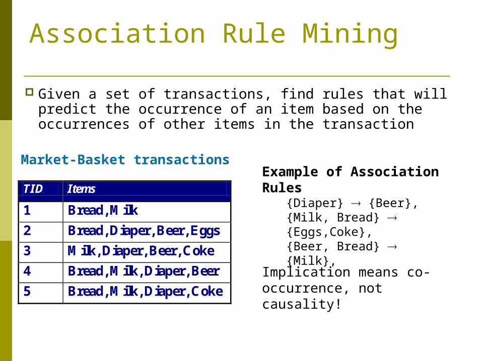
Given a set of transactions, find rules that will predict the occurrence of an item based on the occurrences of other items in the transaction
Market-Basket transactions
TID Items
1 Bread, Milk
2 Bread, Diaper, Beer, Eggs
3 Milk, Diaper, Beer, Coke
4 Bread, Milk, Diaper, Beer
5 Bread, Milk, Diaper, Coke
Example of Association Rules
{Diaper} {Beer},{Milk, Bread} {Eggs,Coke},{Beer, Bread} {Milk},
Implication means co-occurrence, not causality!
Definition: Frequent Itemset Itemset
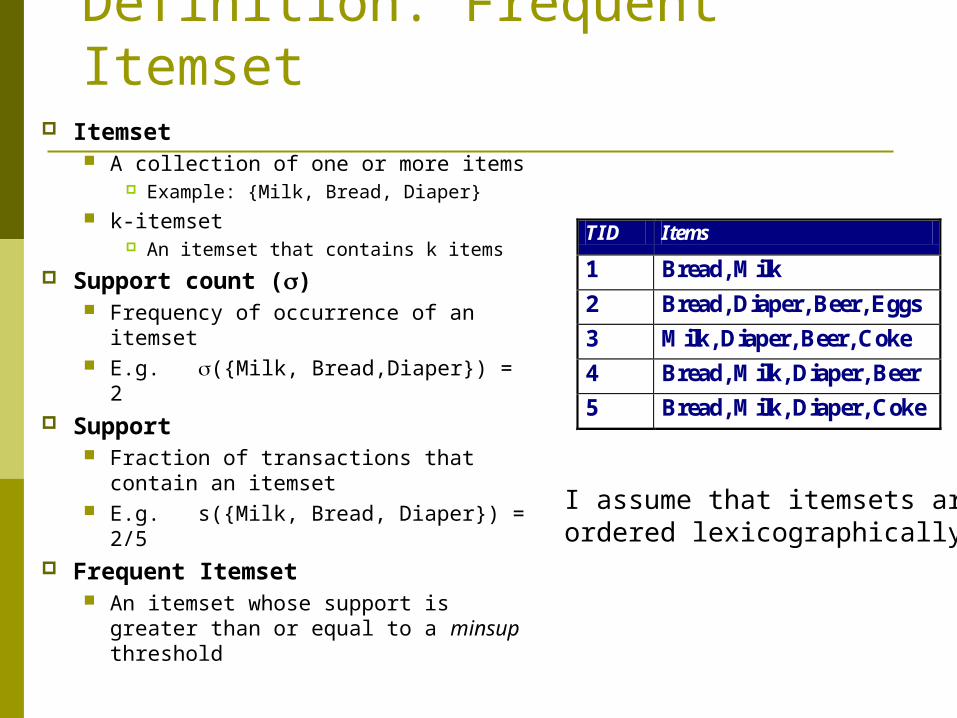
A collection of one or more items Example: {Milk, Bread, Diaper}
k-itemset An itemset that contains k items
Support count () Frequency of occurrence of an
itemset E.g. ({Milk, Bread,Diaper}) = 2
Support Fraction of transactions that
contain an itemset E.g. s({Milk, Bread, Diaper}) = 2/5
Frequent Itemset An itemset whose support is
greater than or equal to a minsup threshold
TID Items
1 Bread, Milk
2 Bread, Diaper, Beer, Eggs
3 Milk, Diaper, Beer, Coke
4 Bread, Milk, Diaper, Beer
5 Bread, Milk, Diaper, Coke
I assume that itemsets are ordered lexicographically
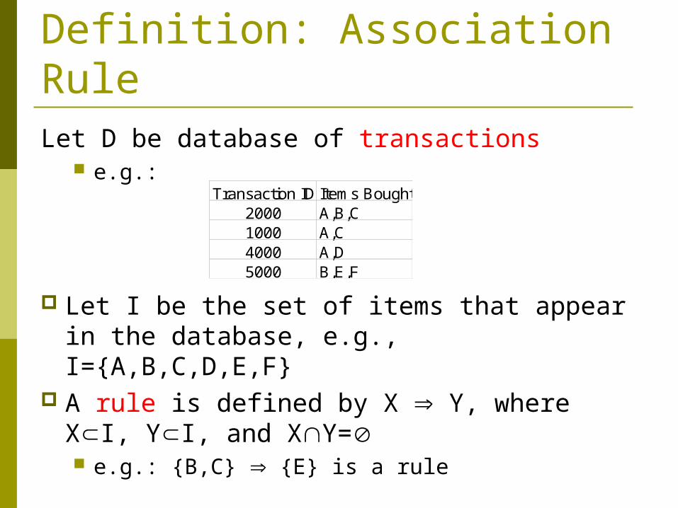
Definition: Association RuleLet D be database of transactions e.g.:
Let I be the set of items that appear in the database, e.g., I={A,B,C,D,E,F}
A rule is defined by X Y, where XI, YI, and XY= e.g.: {B,C} {E} is a rule
Transaction ID Items Bought2000 A,B,C1000 A,C4000 A,D5000 B,E,F
Definition: Association Rule
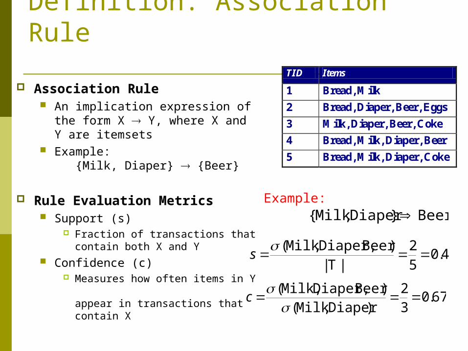
Example:Beer}Diaper,Milk{
4.052
|T|)BeerDiaper,,Milk( s
67.032
)Diaper,Milk()BeerDiaper,Milk,(
c
Association Rule An implication expression of the
form X Y, where X and Y are itemsets
Example: {Milk, Diaper} {Beer}
Rule Evaluation Metrics Support (s)
Fraction of transactions that contain both X and Y
Confidence (c) Measures how often items in Y
appear in transactions thatcontain X
TID Items
1 Bread, Milk
2 Bread, Diaper, Beer, Eggs
3 Milk, Diaper, Beer, Coke
4 Bread, Milk, Diaper, Beer
5 Bread, Milk, Diaper, Coke
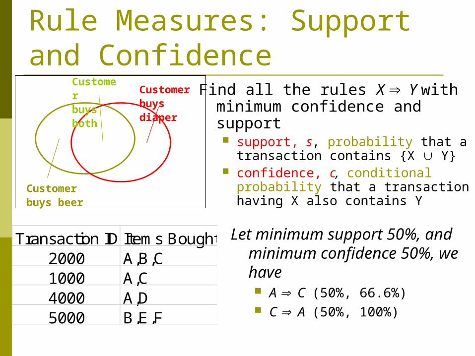
Rule Measures: Support and Confidence
Find all the rules X Y with minimum confidence and support support, s, probability that a
transaction contains {X Y} confidence, c, conditional
probability that a transaction having X also contains Y
Transaction ID Items Bought2000 A,B,C1000 A,C4000 A,D5000 B,E,F
Let minimum support 50%, and minimum confidence 50%, we have A C (50%, 66.6%) C A (50%, 100%)
Customerbuys diaper
Customerbuys both
Customerbuys beer
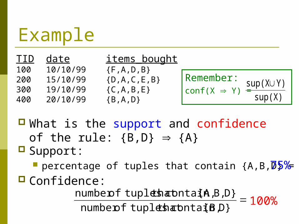
TID date items_bought100 10/10/99 {F,A,D,B}200 15/10/99 {D,A,C,E,B}300 19/10/99 {C,A,B,E}400 20/10/99 {B,A,D}
Example
What is the support and confidence of the rule: {B,D} {A}
Support: percentage of tuples that contain {A,B,D} =
Confidence:
D}{B,contain that tuplesofnumber
D}B,{A,contain that tuplesofnumber
75%
100%
Remember:conf(X Y) =
sup(X)
Y) sup(X

Association Rule Mining TaskGiven a set of transactions T, the goal of
association rule mining is to find all rules having support ≥ minsup threshold confidence ≥ minconf threshold
Brute-force approach: List all possible association rules Compute the support and confidence for each
rule Prune rules that fail the minsup and minconf
thresholds Computationally prohibitive!
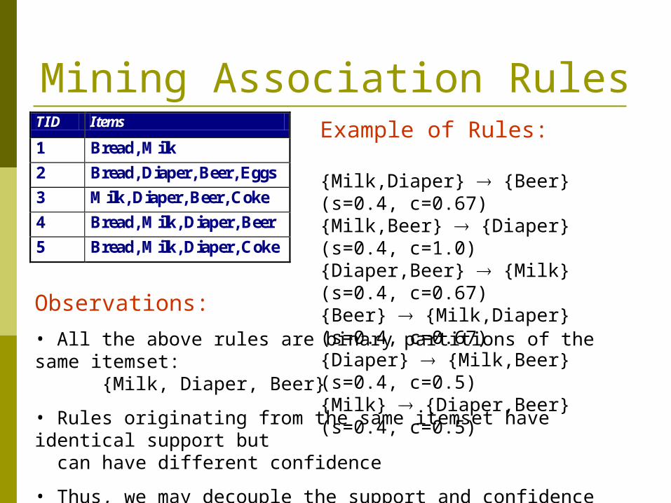
Mining Association RulesExample of Rules:
{Milk,Diaper} {Beer} (s=0.4, c=0.67){Milk,Beer} {Diaper} (s=0.4, c=1.0){Diaper,Beer} {Milk} (s=0.4, c=0.67){Beer} {Milk,Diaper} (s=0.4, c=0.67) {Diaper} {Milk,Beer} (s=0.4, c=0.5) {Milk} {Diaper,Beer} (s=0.4, c=0.5)
TID Items
1 Bread, Milk
2 Bread, Diaper, Beer, Eggs
3 Milk, Diaper, Beer, Coke
4 Bread, Milk, Diaper, Beer
5 Bread, Milk, Diaper, Coke
Observations:
• All the above rules are binary partitions of the same itemset: {Milk, Diaper, Beer}
• Rules originating from the same itemset have identical support but can have different confidence
• Thus, we may decouple the support and confidence requirements

Mining Association Rules Two-step approach:
1. Frequent Itemset Generation– Generate all itemsets whose support minsup
2. Rule Generation– Generate high confidence rules from each frequent
itemset, where each rule is a binary partitioning of a frequent itemset
Frequent itemset generation is still computationally expensive
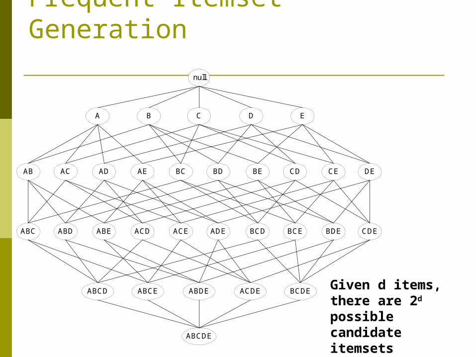
Frequent Itemset Generation
null
AB AC AD AE BC BD BE CD CE DE
A B C D E
ABC ABD ABE ACD ACE ADE BCD BCE BDE CDE
ABCD ABCE ABDE ACDE BCDE
ABCDE
Given d items, there are 2d possible candidate itemsets
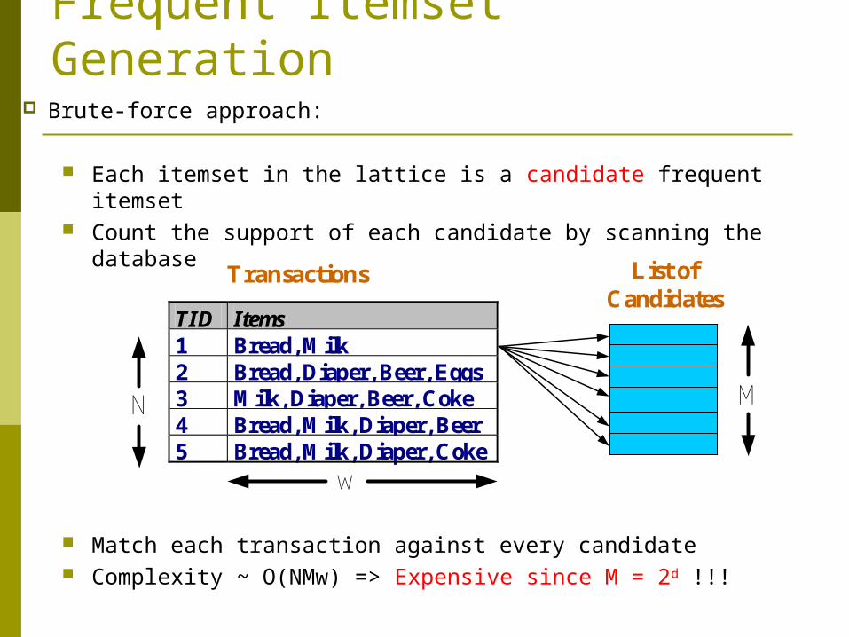
Frequent Itemset Generation Brute-force approach:
Each itemset in the lattice is a candidate frequent itemset Count the support of each candidate by scanning the
database
Match each transaction against every candidate Complexity ~ O(NMw) => Expensive since M = 2d !!!
TID Items 1 Bread, Milk 2 Bread, Diaper, Beer, Eggs 3 Milk, Diaper, Beer, Coke 4 Bread, Milk, Diaper, Beer 5 Bread, Milk, Diaper, Coke
N
Transactions List ofCandidates
M
w

Computational ComplexityGiven d unique items: Total number of itemsets = 2d
Total number of possible association rules:
123 1
1
1 1
dd
d
k
kd
j j
kd
k
dR
If d=6, R = 602 rules
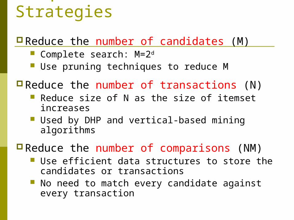
Frequent Itemset Generation Strategies
Reduce the number of candidates (M) Complete search: M=2d
Use pruning techniques to reduce M
Reduce the number of transactions (N) Reduce size of N as the size of itemset increases Used by DHP and vertical-based mining
algorithms
Reduce the number of comparisons (NM) Use efficient data structures to store the
candidates or transactions No need to match every candidate against every
transaction

Reducing Number of Candidates
Apriori principle: If an itemset is frequent, then all of its subsets
must also be frequent
Apriori principle holds due to the following property of the support measure:
Support of an itemset never exceeds the support of its subsets
This is known as the anti-monotone property of support
)()()(:, YsXsYXYX

Example
TID Items
1 Bread, Milk
2 Bread, Diaper, Beer, Eggs
3 Milk, Diaper, Beer, Coke
4 Bread, Milk, Diaper, Beer
5 Bread, Milk, Diaper, Coke
s(Bread) > s(Bread, Beer)
s(Milk) > s(Bread, Milk)
s(Diaper, Beer) > s(Diaper, Beer, Coke)
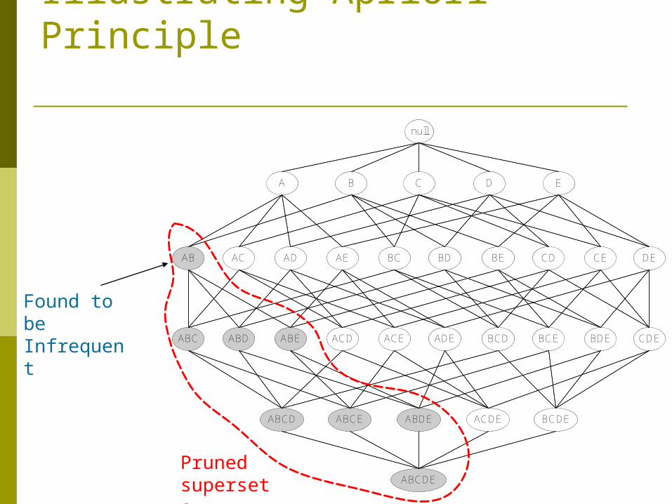
Found to be Infrequent
null
AB AC AD AE BC BD BE CD CE DE
A B C D E
ABC ABD ABE ACD ACE ADE BCD BCE BDE CDE
ABCD ABCE ABDE ACDE BCDE
ABCDE
Illustrating Apriori Principle
null
AB AC AD AE BC BD BE CD CE DE
A B C D E
ABC ABD ABE ACD ACE ADE BCD BCE BDE CDE
ABCD ABCE ABDE ACDE BCDE
ABCDEPruned supersets
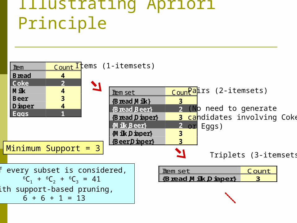
Illustrating Apriori Principle
Item CountBread 4Coke 2Milk 4Beer 3Diaper 4Eggs 1
Itemset Count{Bread,Milk} 3{Bread,Beer} 2{Bread,Diaper} 3{Milk,Beer} 2{Milk,Diaper} 3{Beer,Diaper} 3
Itemset Count {Bread,Milk,Diaper} 3
Items (1-itemsets)
Pairs (2-itemsets)
(No need to generatecandidates involving Cokeor Eggs)
Triplets (3-itemsets)Minimum Support = 3
If every subset is considered, 6C1 + 6C2 + 6C3 = 41
With support-based pruning,6 + 6 + 1 = 13

The Apriori Algorithm (the general idea)
1. Find frequent 1-items and put them to Lk (k=1)
2. Use Lk to generate a collection of candidate itemsets Ck+1 with size (k+1)
3. Scan the database to find which itemsets in Ck+1 are frequent and put them into Lk+1
4. If Lk+1 is not empty k=k+1 GOTO 2
R. Agrawal, R. Srikant: "Fast Algorithms for Mining Association Rules",
Proc. of the 20th Int'l Conference on Very Large Databases, Santiago, Chile, Sept. 1994.
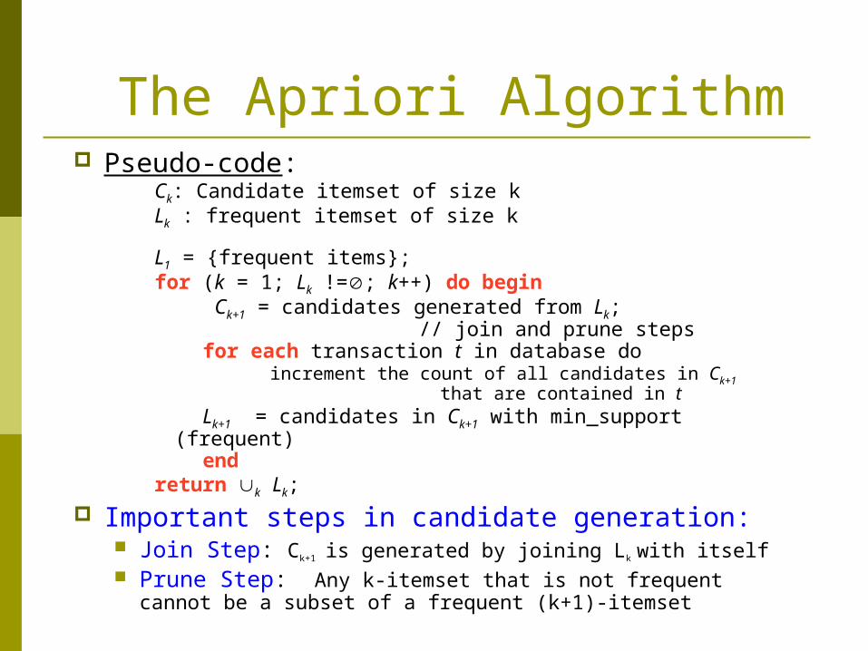
The Apriori Algorithm Pseudo-code:
Ck: Candidate itemset of size kLk : frequent itemset of size k
L1 = {frequent items};for (k = 1; Lk !=; k++) do begin Ck+1 = candidates generated from Lk; // join and prune steps for each transaction t in database do
increment the count of all candidates in Ck+1 that are contained in t
Lk+1 = candidates in Ck+1 with min_support (frequent) endreturn k Lk;
Important steps in candidate generation: Join Step: Ck+1 is generated by joining Lk with itself Prune Step: Any k-itemset that is not frequent cannot be
a subset of a frequent (k+1)-itemset
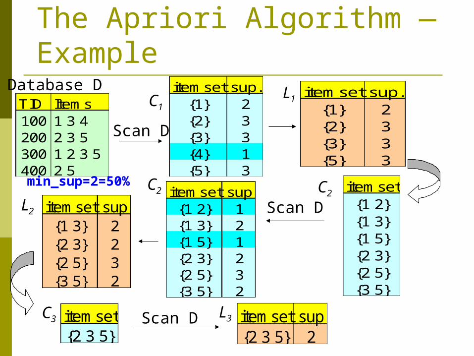
The Apriori Algorithm — Example
TID Items100 1 3 4200 2 3 5300 1 2 3 5400 2 5
Database D itemset sup.{1} 2{2} 3{3} 3{4} 1{5} 3
itemset sup.{1} 2{2} 3{3} 3{5} 3
Scan D
C1L1
itemset{1 2}{1 3}{1 5}{2 3}{2 5}{3 5}
itemset sup{1 2} 1{1 3} 2{1 5} 1{2 3} 2{2 5} 3{3 5} 2
itemset sup{1 3} 2{2 3} 2{2 5} 3{3 5} 2
L2
C2 C2
Scan D
C3 L3itemset{2 3 5}
Scan D itemset sup{2 3 5} 2
min_sup=2=50%
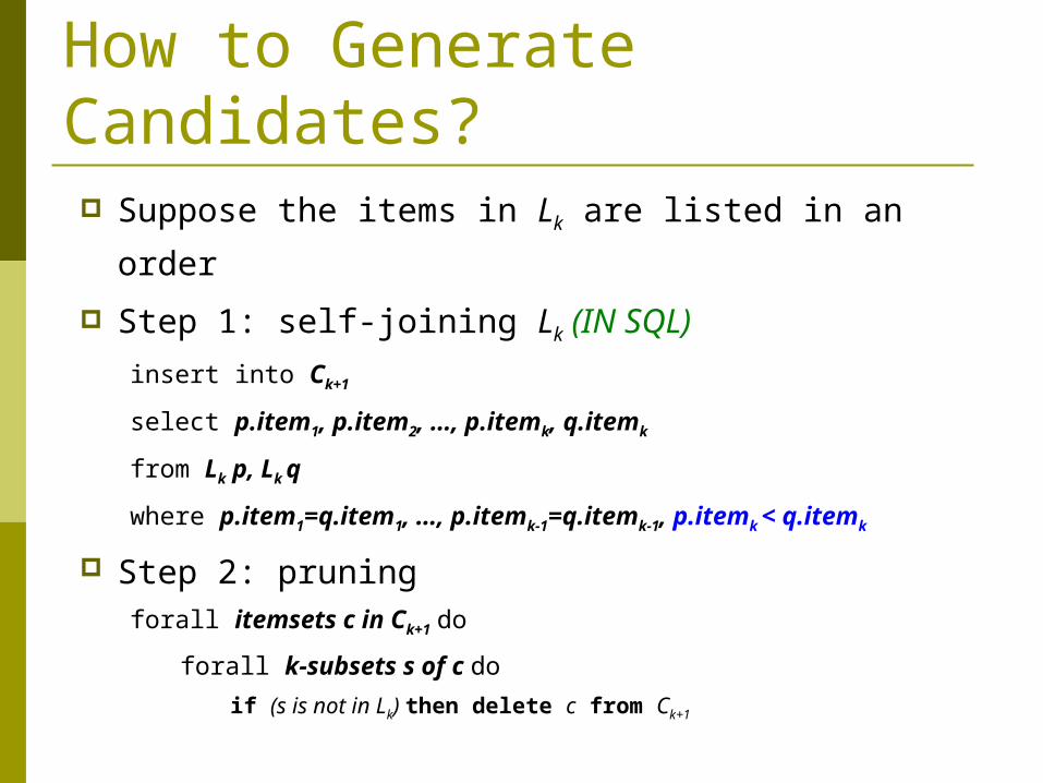
How to Generate Candidates? Suppose the items in Lk are listed in an order
Step 1: self-joining Lk (IN SQL)
insert into Ck+1
select p.item1, p.item2, …, p.itemk, q.itemk
from Lk p, Lk q
where p.item1=q.item1, …, p.itemk-1=q.itemk-1, p.itemk <
q.itemk
Step 2: pruningforall itemsets c in Ck+1 do
forall k-subsets s of c do
if (s is not in Lk) then delete c from Ck+1
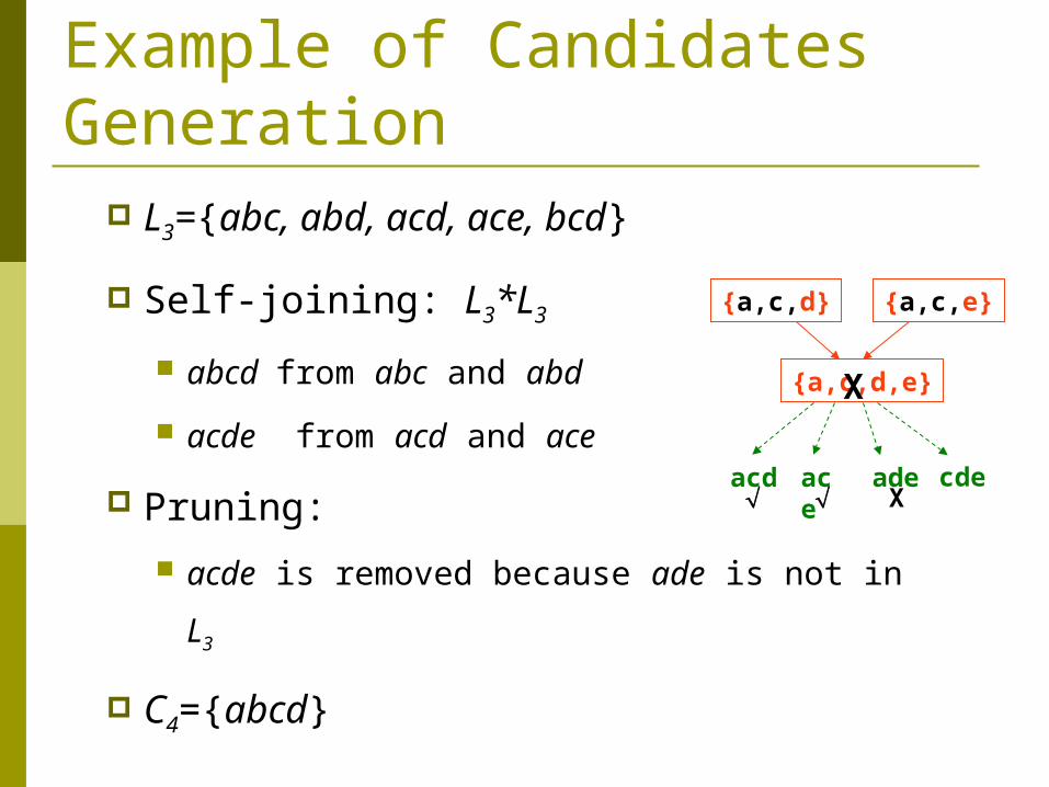
Example of Candidates Generation L3={abc, abd, acd, ace, bcd}
Self-joining: L3*L3
abcd from abc and abd
acde from acd and ace
Pruning:
acde is removed because ade is not in L3
C4={abcd}
{a,c,d} {a,c,e}
{a,c,d,e}
acd ace
ade cde X
X
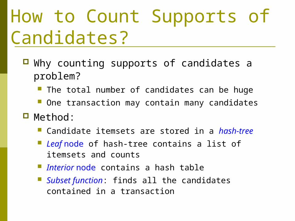
How to Count Supports of Candidates? Why counting supports of candidates a problem?
The total number of candidates can be huge One transaction may contain many candidates
Method: Candidate itemsets are stored in a hash-tree Leaf node of hash-tree contains a list of itemsets and
counts Interior node contains a hash table Subset function: finds all the candidates contained in a
transaction
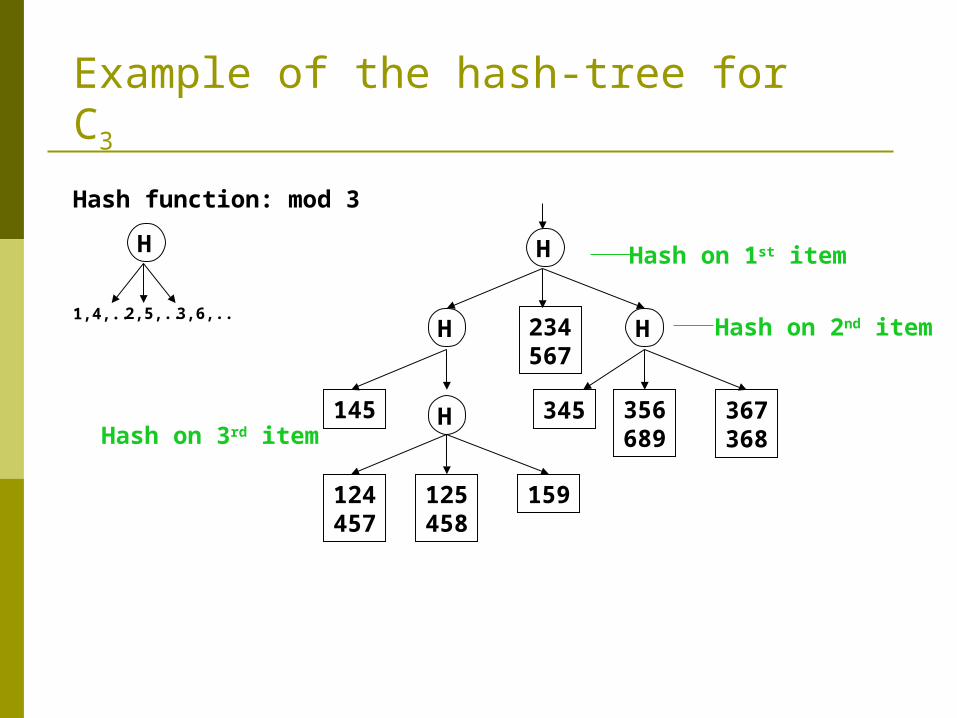
Example of the hash-tree for C3
Hash function: mod 3
H
1,4,.. 2,5,.. 3,6,..
H Hash on 1st item
H H234567
H145
124457
125458
159
345 356689
367368
Hash on 2nd item
Hash on 3rd item

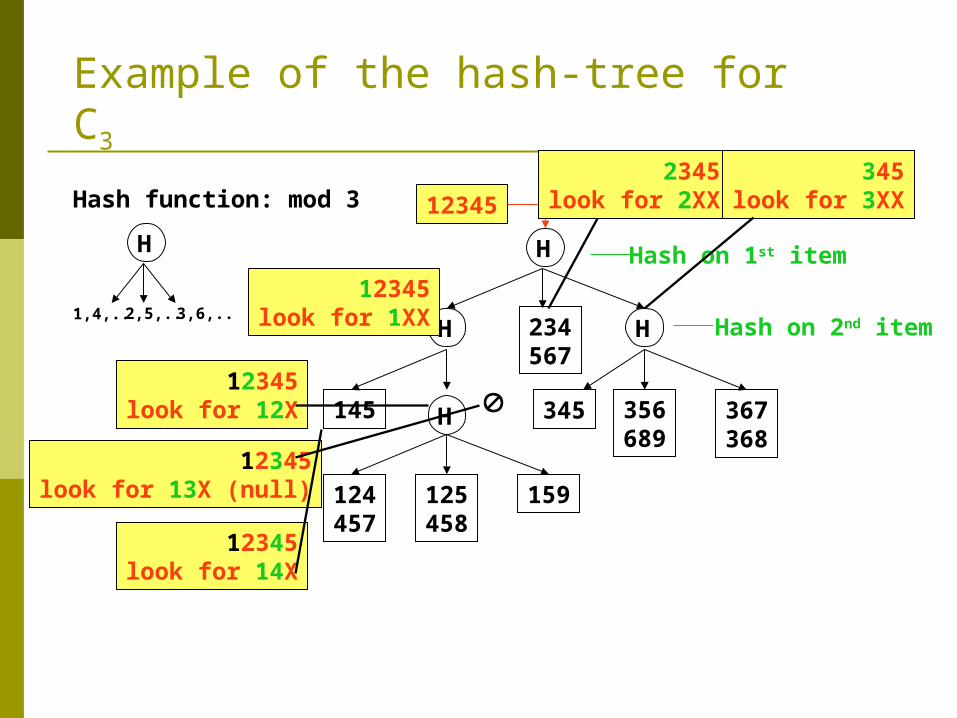
Example of the hash-tree for C3
Hash function: mod 3
H
1,4,.. 2,5,.. 3,6,..
H Hash on 1st item
H H234567
H145
124457
125458
159
345 356689
367368
Hash on 2nd item
Hash on 3rd item
12345
12345look for 1XX
2345look for 2XX
345look for 3XX
Example of the hash-tree for C3
Hash function: mod 3
H
1,4,.. 2,5,.. 3,6,..
H Hash on 1st item
H H234567
H145
124457
125458
159
345 356689
367368
Hash on 2nd item
12345
12345look for 1XX
2345look for 2XX
345look for 3XX
12345look for 12X
12345look for 13X (null)
12345look for 14X
AprioriTid: Use D only for first pass The database is not used after the 1st pass. Instead, the set Ck’ is used for each step, Ck’ =
<TID, {Xk}> : each Xk is a potentially frequent itemset in transaction with id=TID.
At each step Ck’ is generated from Ck-1’ at the pruning step of constructing Ck and used to compute Lk.
For small values of k, Ck’ could be larger than the database!
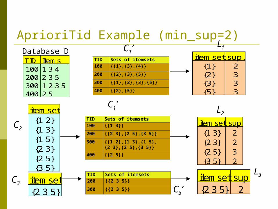
AprioriTid Example (min_sup=2)
TID Items100 1 3 4200 2 3 5300 1 2 3 5400 2 5
Database Ditemset sup.
{1} 2{2} 3{3} 3{5} 3
L1
itemset{1 2}{1 3}{1 5}{2 3}{2 5}{3 5}
itemset sup{1 3} 2{2 3} 2{2 5} 3{3 5} 2
L2
C2
C3’itemset{2 3 5}
itemset sup{2 3 5} 2
TID Sets of itemsets100 {{1},{3},{4}}
200 {{2},{3},{5}}
300 {{1},{2},{3},{5}}
400 {{2},{5}}
C1’
TID Sets of itemsets100 {{1 3}}
200 {{2 3},{2 5},{3 5}}
300 {{1 2},{1 3},{1 5}, {2 3},{2 5},{3 5}}
400 {{2 5}}
C1’
C3
TID Sets of itemsets200 {{2 3 5}}
300 {{2 3 5}}
L3
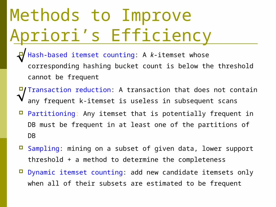
Methods to Improve Apriori’s Efficiency Hash-based itemset counting: A k-itemset whose
corresponding hashing bucket count is below the threshold
cannot be frequent
Transaction reduction: A transaction that does not contain
any frequent k-itemset is useless in subsequent scans
Partitioning: Any itemset that is potentially frequent in DB
must be frequent in at least one of the partitions of DB
Sampling: mining on a subset of given data, lower support
threshold + a method to determine the completeness
Dynamic itemset counting: add new candidate itemsets
only when all of their subsets are estimated to be frequent

Maximal Frequent Itemset
null
AB AC AD AE BC BD BE CD CE DE
A B C D E
ABC ABD ABE ACD ACE ADE BCD BCE BDE CDE
ABCD ABCE ABDE ACDE BCDE
ABCDE
Border
Infrequent Itemsets
Maximal Itemsets
An itemset is maximal frequent if none of its immediate supersets is frequent
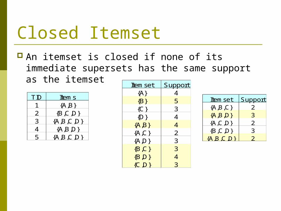
Closed Itemset An itemset is closed if none of its immediate
supersets has the same support as the itemset
TID Items1 {A,B}2 {B,C,D}3 {A,B,C,D}4 {A,B,D}5 {A,B,C,D}
Itemset Support{A} 4{B} 5{C} 3{D} 4
{A,B} 4{A,C} 2{A,D} 3{B,C} 3{B,D} 4{C,D} 3
Itemset Support{A,B,C} 2{A,B,D} 3{A,C,D} 2{B,C,D} 3
{A,B,C,D} 2
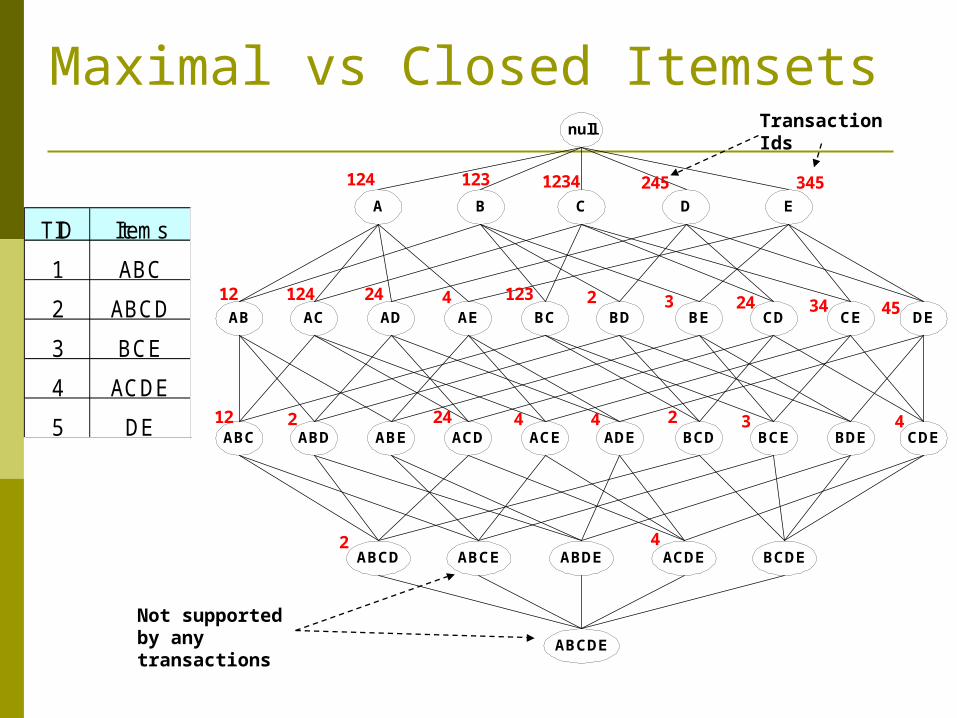
Maximal vs Closed Itemsets
TID Items
1 ABC
2 ABCD
3 BCE
4 ACDE
5 DE
null
AB AC AD AE BC BD BE CD CE DE
A B C D E
ABC ABD ABE ACD ACE ADE BCD BCE BDE CDE
ABCD ABCE ABDE ACDE BCDE
ABCDE
124 123 1234 245 345
12 124 24 4 123 2 3 24 34 45
12 2 24 4 4 2 3 4
2 4
Transaction Ids
Not supported by any transactions
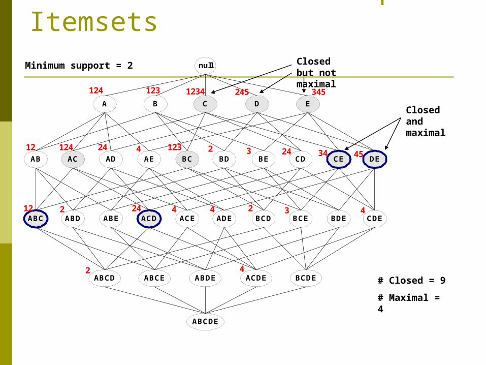
Maximal vs Closed Frequent Itemsets
null
AB AC AD AE BC BD BE CD CE DE
A B C D E
ABC ABD ABE ACD ACE ADE BCD BCE BDE CDE
ABCD ABCE ABDE ACDE BCDE
ABCDE
124 123 1234 245 345
12 124 24 4 123 2 3 24 34 45
12 2 24 4 4 2 3 4
2 4
Minimum support = 2
# Closed = 9
# Maximal = 4
Closed and maximal
Closed but not maximal

Maximal vs Closed Itemsets
FrequentItemsets
ClosedFrequentItemsets
MaximalFrequentItemsets

Factors Affecting Complexity Choice of minimum support threshold
lowering support threshold results in more frequent itemsets
this may increase number of candidates and max length of frequent itemsets
Dimensionality (number of items) of the data set more space is needed to store support count of each item if number of frequent items also increases, both
computation and I/O costs may also increase Size of database
since Apriori makes multiple passes, run time of algorithm may increase with number of transactions
Average transaction width transaction width increases with denser data sets This may increase max length of frequent itemsets and
traversals of hash tree (number of subsets in a transaction increases with its width)
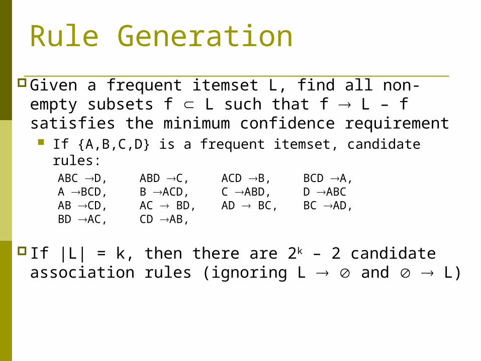
Rule Generation
Given a frequent itemset L, find all non-empty subsets f L such that f L – f satisfies the minimum confidence requirement If {A,B,C,D} is a frequent itemset, candidate rules:
ABC D, ABD C, ACD B, BCD A, A BCD, B ACD, C ABD, D ABCAB CD, AC BD, AD BC, BC AD, BD AC, CD AB,
If |L| = k, then there are 2k – 2 candidate association rules (ignoring L and L)

Rule GenerationHow to efficiently generate rules from frequent
itemsets? In general, confidence does not have an anti-
monotone propertyc(ABC D) can be larger or smaller than c(AB D)
But confidence of rules generated from the same itemset has an anti-monotone property
e.g., L = {A,B,C,D}:
c(ABC D) c(AB CD) c(A BCD) Confidence is anti-monotone w.r.t. number of items on the RHS of the rule
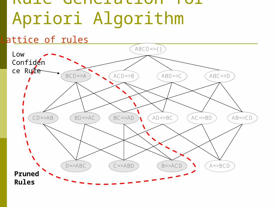
Rule Generation for Apriori Algorithm
ABCD=>{ }
BCD=>A ACD=>B ABD=>C ABC=>D
BC=>ADBD=>ACCD=>AB AD=>BC AC=>BD AB=>CD
D=>ABC C=>ABD B=>ACD A=>BCD
Lattice of rulesABCD=>{ }
BCD=>A ACD=>B ABD=>C ABC=>D
BC=>ADBD=>ACCD=>AB AD=>BC AC=>BD AB=>CD
D=>ABC C=>ABD B=>ACD A=>BCD
Pruned Rules
Low Confidence Rule

Rule Generation for Apriori AlgorithmCandidate rule is generated by merging two
rules that share the same prefixin the rule consequent
join(CD=>AB,BD=>AC)would produce the candidaterule D => ABC
Prune rule D=>ABC if itssubset AD=>BC does not havehigh confidence
BD=>ACCD=>AB
D=>ABC

Is Apriori Fast Enough? — Performance Bottlenecks
The core of the Apriori algorithm: Use frequent (k – 1)-itemsets to generate candidate frequent k-
itemsets Use database scan and pattern matching to collect counts for
the candidate itemsets
The bottleneck of Apriori: candidate generation Huge candidate sets:
104 frequent 1-itemset will generate 107 candidate 2-itemsets
To discover a frequent pattern of size 100, e.g., {a1, a2, …, a100}, one needs to generate 2100 1030 candidates.
Multiple scans of database: Needs (n +1 ) scans, n is the length of the longest pattern

FP-growth: Mining Frequent Patterns Without Candidate Generation
Compress a large database into a compact, Frequent-Pattern tree (FP-tree) structure highly condensed, but complete for frequent pattern
mining avoid costly database scans
Develop an efficient, FP-tree-based frequent pattern mining method A divide-and-conquer methodology: decompose mining
tasks into smaller ones Avoid candidate generation: sub-database test only!
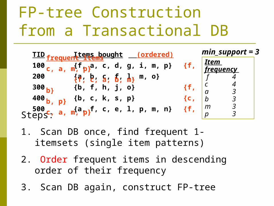
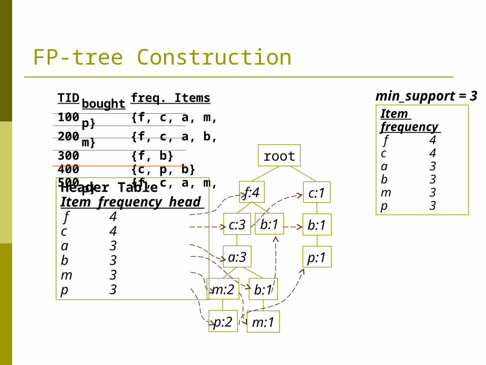
FP-tree Construction from a Transactional DB
Item frequency f 4c 4a 3b 3m 3p 3
min_support = 3TID Items bought (ordered) frequent items100 {f, a, c, d, g, i, m, p} {f, c, a, m, p}200 {a, b, c, f, l, m, o} {f, c, a, b, m}300 {b, f, h, j, o} {f, b}400 {b, c, k, s, p} {c, b, p}500 {a, f, c, e, l, p, m, n} {f, c, a, m, p}
Steps:
1. Scan DB once, find frequent 1-itemsets (single item patterns)
2. Order frequent items in descending order of their frequency
3. Scan DB again, construct FP-tree

FP-tree Construction
root
TID freq. Items bought100 {f, c, a, m, p}200 {f, c, a, b, m}300 {f, b}400 {c, p, b}500 {f, c, a, m, p}
Item frequency f 4c 4a 3b 3m 3p 3
min_support = 3
f:1
c:1
a:1
m:1
p:1

FP-tree Construction
root
Item frequency f 4c 4a 3b 3m 3p 3
min_support = 3
f:2
c:2
a:2
m:1
p:1
b:1
m:1
TID freq. Items bought100 {f, c, a, m, p}200 {f, c, a, b, m}300 {f, b}400 {c, p, b}500 {f, c, a, m, p}

FP-tree Construction
root
Item frequency f 4c 4a 3b 3m 3p 3
min_support = 3
f:3
c:2
a:2
m:1
p:1
b:1
m:1
b:1
TID freq. Items bought100 {f, c, a, m, p}200 {f, c, a, b, m}300 {f, b}400 {c, p, b}500 {f, c, a, m, p}
c:1
b:1
p:1
FP-tree Construction
root
Item frequency f 4c 4a 3b 3m 3p 3
min_support = 3
f:4
c:3
a:3
m:2
p:2
b:1
m:1
b:1
TID freq. Items bought100 {f, c, a, m, p}200 {f, c, a, b, m}300 {f, b}400 {c, p, b}500 {f, c, a, m, p}
c:1
b:1
p:1
Header TableItem frequency head f 4c 4a 3b 3m 3p 3
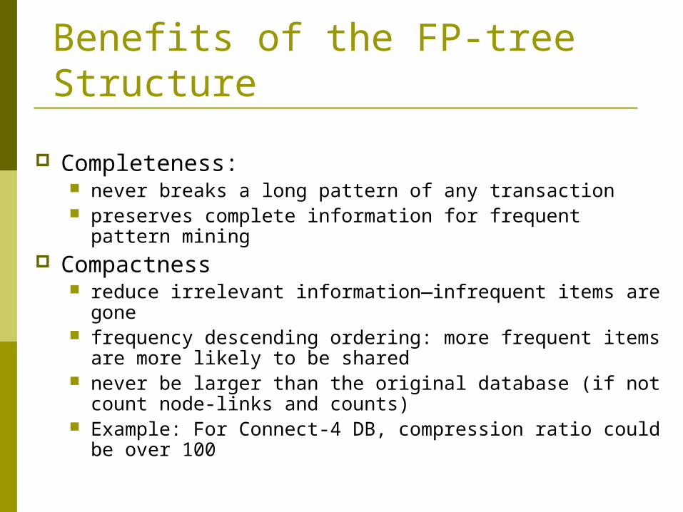
Benefits of the FP-tree Structure
Completeness: never breaks a long pattern of any transaction preserves complete information for frequent pattern mining
Compactness reduce irrelevant information—infrequent items are gone frequency descending ordering: more frequent items are
more likely to be shared never be larger than the original database (if not count
node-links and counts) Example: For Connect-4 DB, compression ratio could be
over 100
Mining Frequent Patterns Using FP-tree
General idea (divide-and-conquer) Recursively grow frequent pattern path using the FP-tree
Method For each item, construct its conditional pattern-base, and
then its conditional FP-tree Repeat the process on each newly created conditional FP-
tree Until the resulting FP-tree is empty, or it contains only
one path (single path will generate all the combinations of its sub-paths, each of which is a frequent pattern)
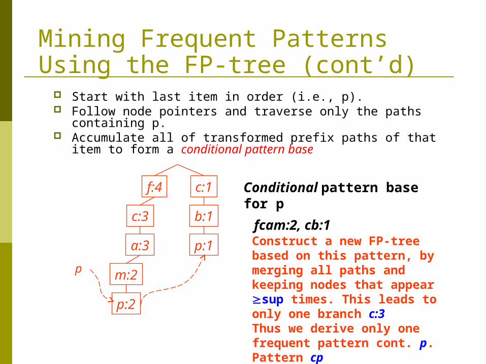
Mining Frequent Patterns Using the FP-tree (cont’d) Start with last item in order (i.e., p). Follow node pointers and traverse only the paths containing p. Accumulate all of transformed prefix paths of that item to form
a conditional pattern base
Conditional pattern base for p
fcam:2, cb:1
f:4
c:3
a:3
m:2
p:2
c:1
b:1
p:1
p
Construct a new FP-tree based on this pattern, by merging all paths and keeping nodes that appear sup times. This leads to only one branch c:3Thus we derive only one frequent pattern cont. p. Pattern cp
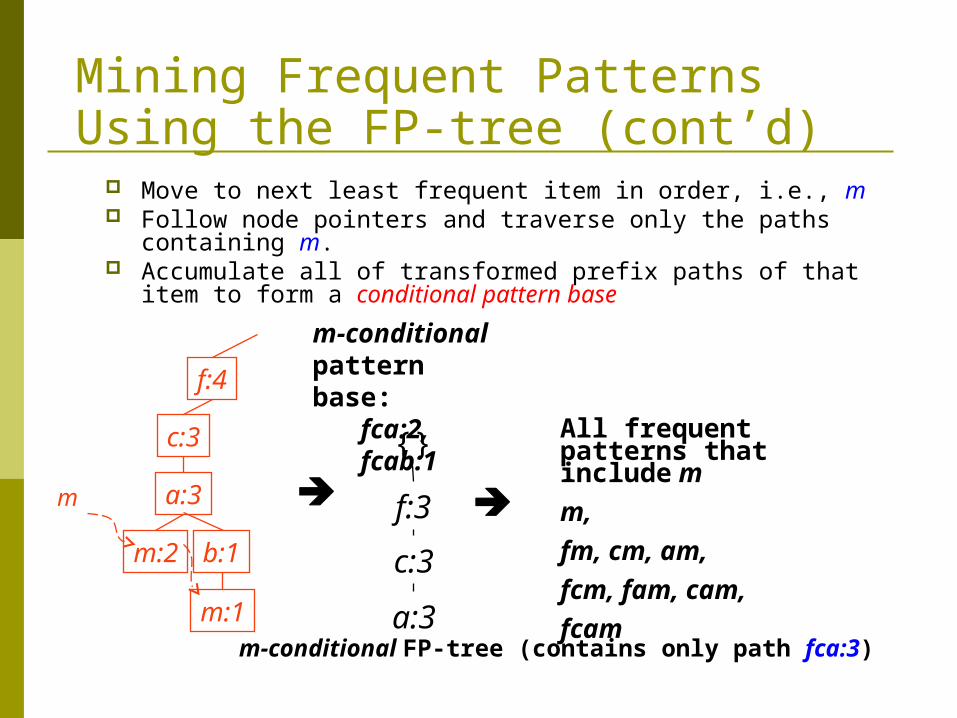
Mining Frequent Patterns Using the FP-tree (cont’d) Move to next least frequent item in order, i.e., m Follow node pointers and traverse only the paths containing m. Accumulate all of transformed prefix paths of that item to form
a conditional pattern base
f:4
c:3
a:3
m:2
m
m:1
b:1
m-conditional pattern base:
fca:2, fcab:1
{}
f:3
c:3
a:3m-conditional FP-tree (contains only path fca:3)
All frequent patterns that include m
m,
fm, cm, am,
fcm, fam, cam,
fcam

Properties of FP-tree for Conditional Pattern Base Construction
Node-link property For any frequent item ai, all the possible frequent patterns
that contain ai can be obtained by following ai's node-links,
starting from ai's head in the FP-tree header
Prefix path property To calculate the frequent patterns for a node ai in a path P,
only the prefix sub-path of ai in P need to be accumulated,
and its frequency count should carry the same count as
node ai.

Conditional Pattern-Bases for the example
EmptyEmptyf
{(f:3)}|c{(f:3)}c
{(f:3, c:3)}|a{(fc:3)}a
Empty{(fca:1), (f:1), (c:1)}b
{(f:3, c:3, a:3)}|m{(fca:2), (fcab:1)}m
{(c:3)}|p{(fcam:2), (cb:1)}p
Conditional FP-treeConditional pattern-baseItem
Why Is Frequent Pattern Growth Fast?
Performance studies show FP-growth is an order of magnitude faster than Apriori,
and is also faster than tree-projection
Reasoning No candidate generation, no candidate test
Uses compact data structure
Eliminates repeated database scan
Basic operation is counting and FP-tree building
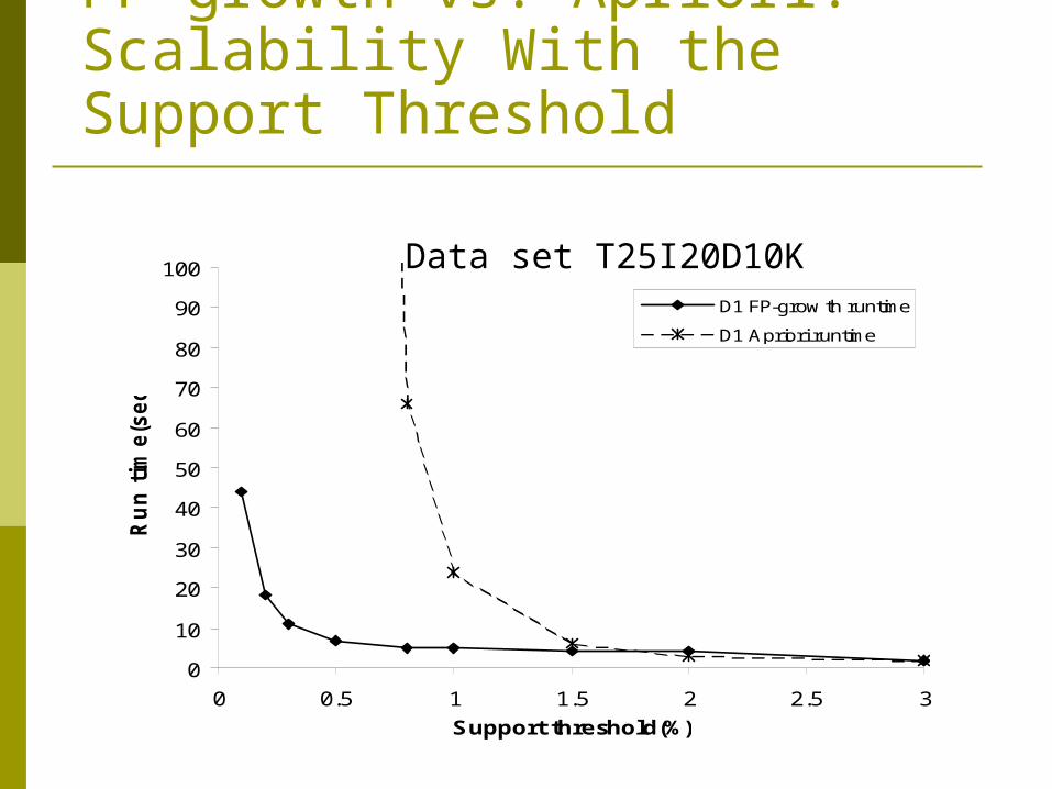
FP-growth vs. Apriori: Scalability With the Support Threshold
0
10
20
30
40
50
60
70
80
90
100
0 0.5 1 1.5 2 2.5 3
Support threshold(%)
Ru
n t
ime(s
ec.)
D1 FP-grow th runtime
D1 Apriori runtime
Data set T25I20D10K