advanced topics in data mining: association rules
TRANSCRIPT

Advanced Topics in Data Mining:
Association Rules
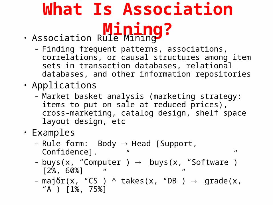
What Is Association Mining?• Association Rule Mining
– Finding frequent patterns, associations, correlations, or causal structures among item sets in transaction databases, relational databases, and other information repositories
• Applications– Market basket analysis (marketing strategy: items to put
on sale at reduced prices), cross-marketing, catalog design, shelf space layout design, etc
• Examples– Rule form: Body ead [Support, Confidence].– buys(x, “Computer”) buys(x, “Software”) [2%, 60%]– major(x, “CS”) ^ takes(x, “DB”) grade(x, “A”) [1%,
75%]
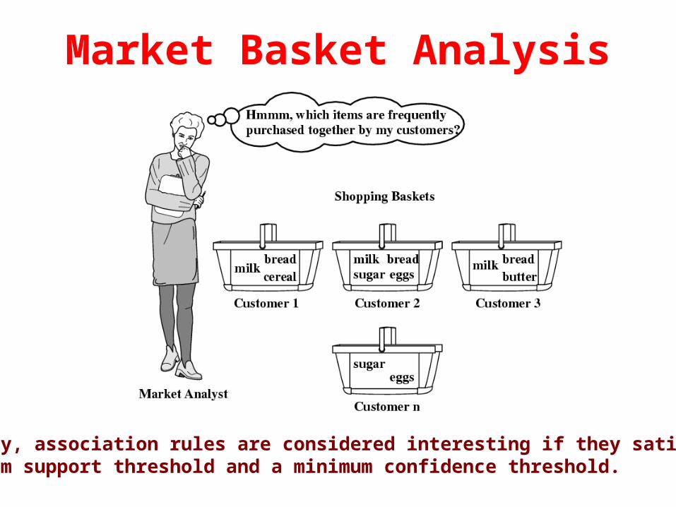
Market Basket Analysis
Typically, association rules are considered interesting if they satisfy both a minimum support threshold and a minimum confidence threshold.

Rule Measures: Support and Confidence
• Let minimum support 50%, and minimum confidence 50%, we have– A C [50%, 66.6%]
– C A [50%, 100%]
Transaction ID Items Bought1000 A,B,C2000 A,C3000 A,D4000 B,E,F

Support & Confidence

Association Rule: Basic Concepts
• Given– (1) database of transactions, – (2) each transaction is a list of items
(purchased by a customer in a visit)
• Find all rules that correlate the presence of one set of items with that of another set of items
• Find all the rules A B with minimum confidence and support– support, s, P(A B)– confidence, c, P(B|A)
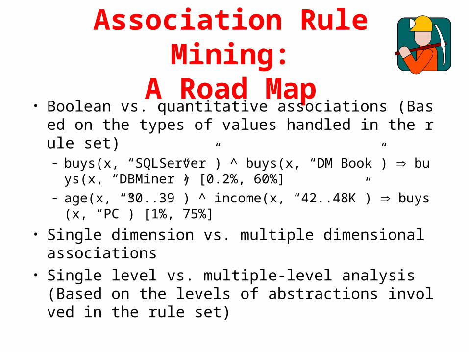
Association Rule Mining:A Road Map
• Boolean vs. quantitative associations (Based on the types of values handled in the rule set)– buys(x, “SQLServer”) ^ buys(x, “DM Book”) buys(x, “
DBMiner”) [0.2%, 60%]– age(x, “30..39”) ^ income(x, “42..48K”) buys(x, “PC”)
[1%, 75%]
• Single dimension vs. multiple dimensional associations
• Single level vs. multiple-level analysis (Based on the levels of abstractions involved in the rule set)
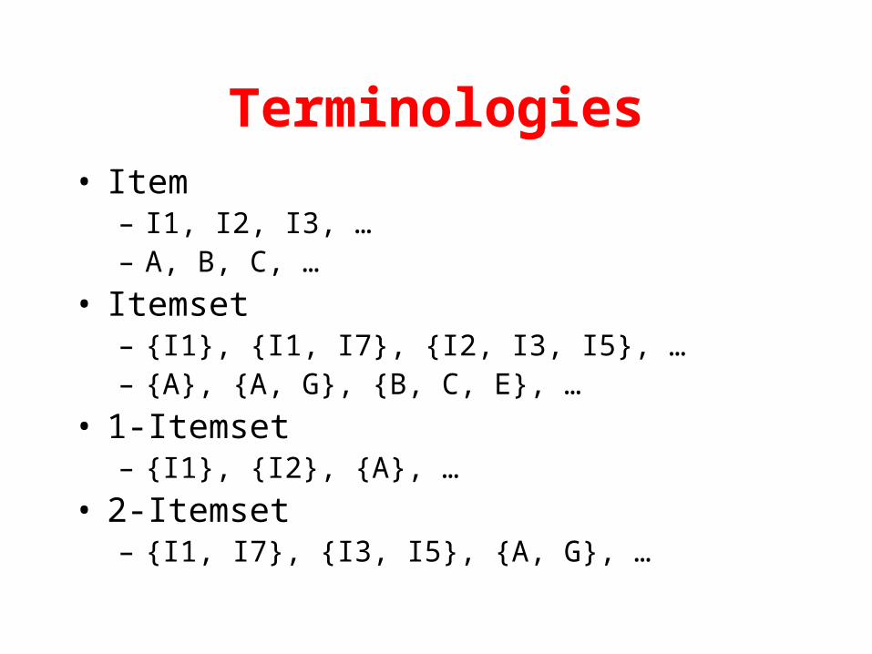
Terminologies• Item
– I1, I2, I3, …– A, B, C, …
• Itemset– {I1}, {I1, I7}, {I2, I3, I5}, …– {A}, {A, G}, {B, C, E}, …
• 1-Itemset– {I1}, {I2}, {A}, …
• 2-Itemset– {I1, I7}, {I3, I5}, {A, G}, …
Terminologies
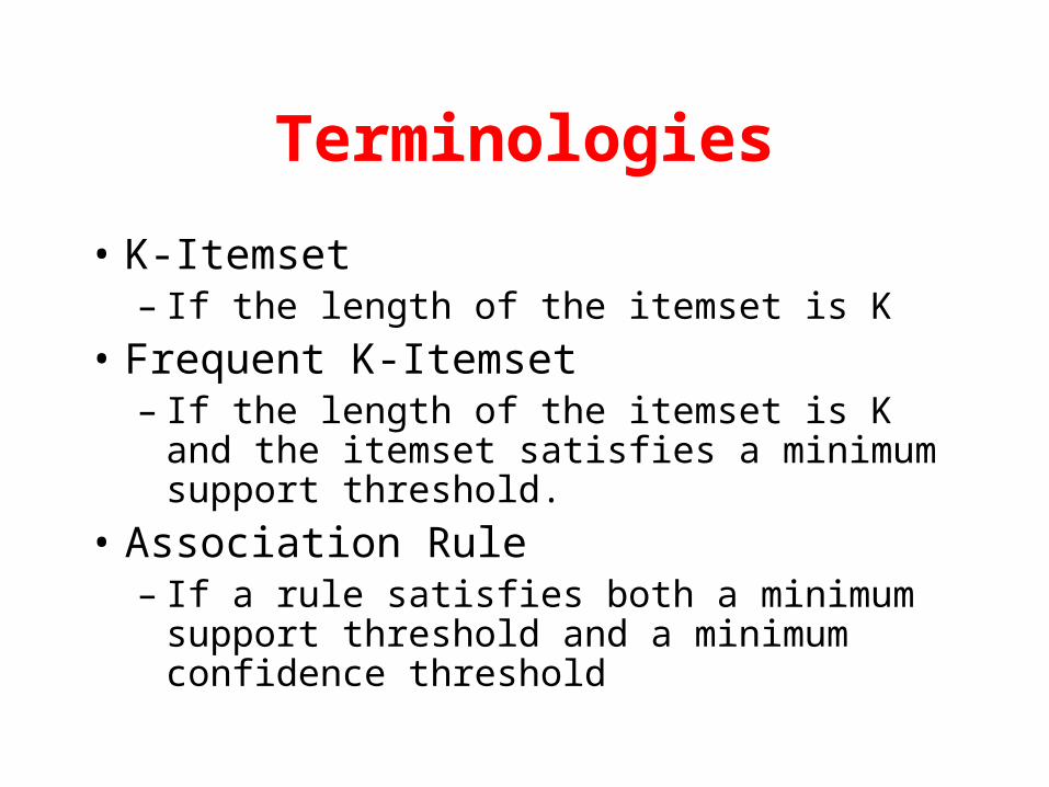
• K-Itemset– If the length of the itemset is K
• Frequent K-Itemset– If the length of the itemset is K and the itemset
satisfies a minimum support threshold.
• Association Rule– If a rule satisfies both a minimum support
threshold and a minimum confidence threshold

Analysis• The number of itemsets of a given cardinality
tends to grow exponentially

Mining Association Rules: Apriori Principle
• For rule A C:– support = support({A C}) = 50%– confidence = support({A C})/support({A}) = 66.6%
• The Apriori principle:– Any subset of a frequent itemset must be frequent
Transaction ID Items Bought1000 A,B,C2000 A,C3000 A,D4000 B,E,F
Frequent Itemset Support{A} 75%{B} 50%{C} 50%
{A,C} 50%
Min. support 50%Min. confidence 50%
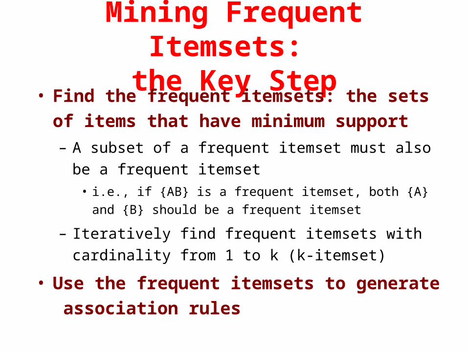
Mining Frequent Itemsets: the Key Step
• Find the frequent itemsets: the sets of items that
have minimum support
– A subset of a frequent itemset must also be a frequent
itemset
• i.e., if {AB} is a frequent itemset, both {A} and {B} should be a
frequent itemset
– Iteratively find frequent itemsets with cardinality from 1 to
k (k-itemset)
• Use the frequent itemsets to generate
association rules

Example
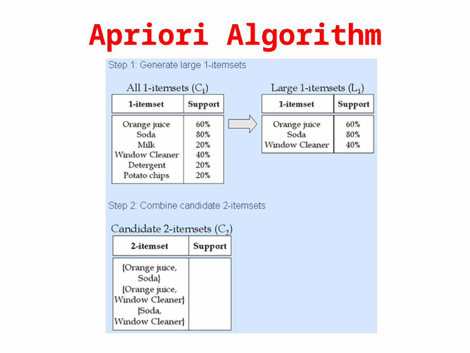
Apriori Algorithm

Apriori Algorithm

Apriori Algorithm
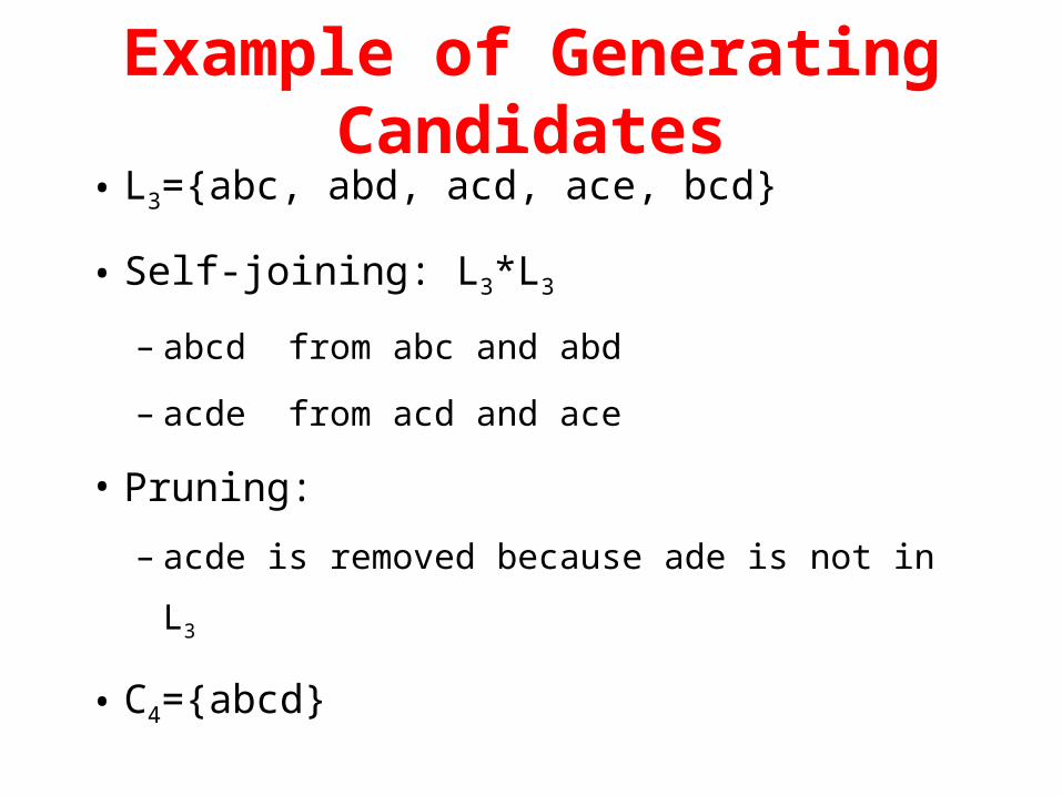
Example of Generating Candidates
• L3={abc, abd, acd, ace, bcd}
• Self-joining: L3*L3
– abcd from abc and abd
– acde from acd and ace
• Pruning:
– acde is removed because ade is not in L3
• C4={abcd}
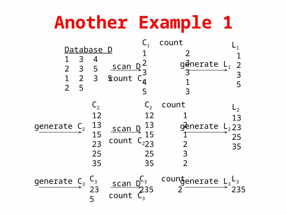
Another Example 1Database D1 3 42 3 51 2 3 52 5
scan D
count C1
C1 count1 22 33 34 15 3
generate L1
L1
1 2 3 5
scan D
count C2
C2 count12 113 215 123 225 335 2
generate L2
L2
13232535
C2
121315232535
generate C2
scan D
count C3
C3 count235 2
generate L3L3
235C3
235generate C3
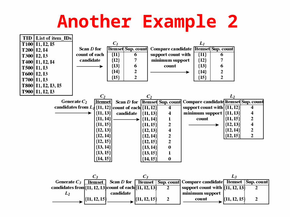
Another Example 2
Is Apriori Fast Enough? — Performance Bottlenecks
• The core of the Apriori algorithm:– Use frequent (k–1)-itemsets to generate candidate frequent k-
itemsets
– Use database scan to collect counts for the candidate itemsets
• The bottleneck of Apriori:– Huge candidate sets:
• 104 frequent 1-itemset will generate 107 candidate 2-itemsets
• To discover a frequent pattern of size 100, e.g., {a1, a2, …, a100}, one needs to generate 2100 1030 candidates.
– Multiple scans of database: • Needs (n +1) scans, n is the length of the longest pattern

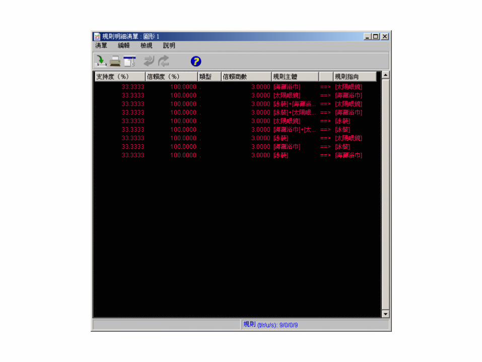
Demo-IBM Intelligent Minner

Demo Database


Methods to Improve Apriori’s Efficiency
• Hash-based itemset counting: A k-itemset whose
corresponding hashing bucket count is below the threshold
cannot be frequent
• Transaction reduction: A transaction that does not contain
any frequent k-itemset is useless in subsequent scans
• Partitioning: Any itemset that is potentially frequent in DB
must be frequent in at least one of the partitions of DB
• Sampling: mining on a subset of given data, lower support
threshold + a method to determine the completeness

Partitioning
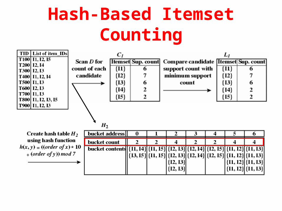
Hash-Based Itemset Counting
= *+

Compare Apriori & DHP (Direct Hash & Pruning)
Apriori
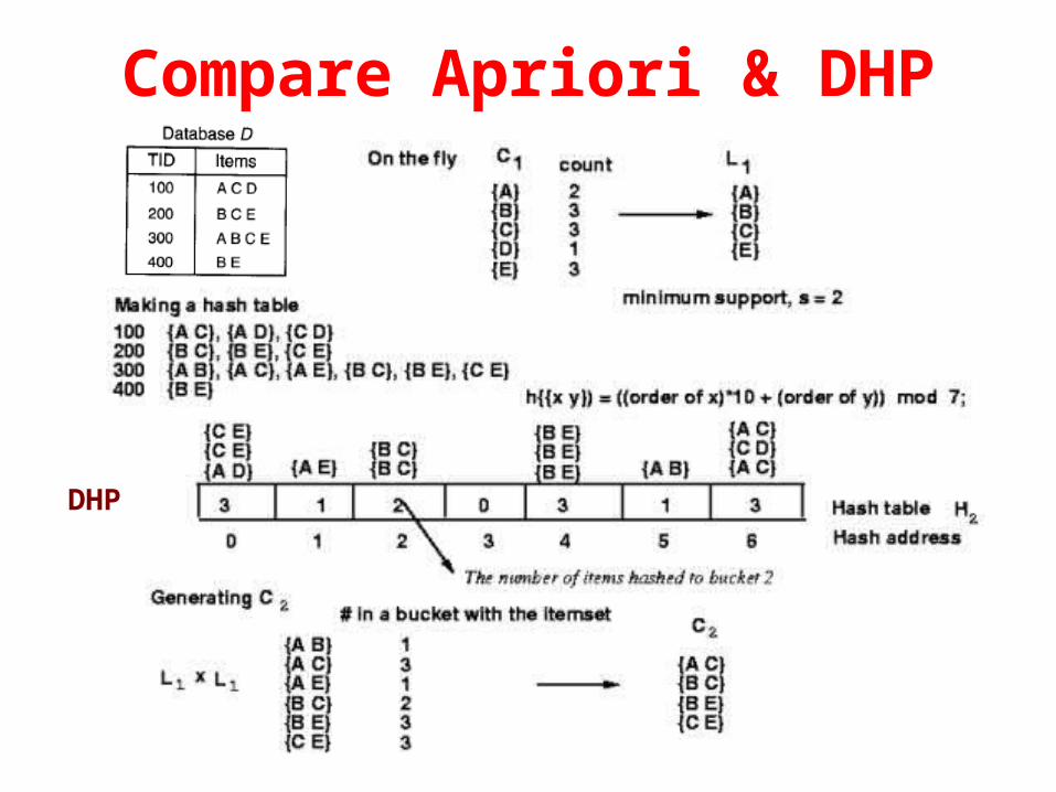
Compare Apriori & DHP
DHP
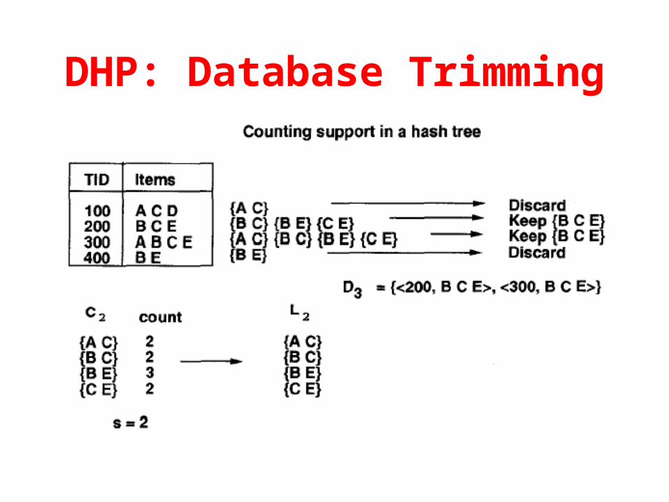
DHP: Database Trimming

DHP (Direct Hash & Pruning)
• A database has four transactions• Let min_sup = 50%
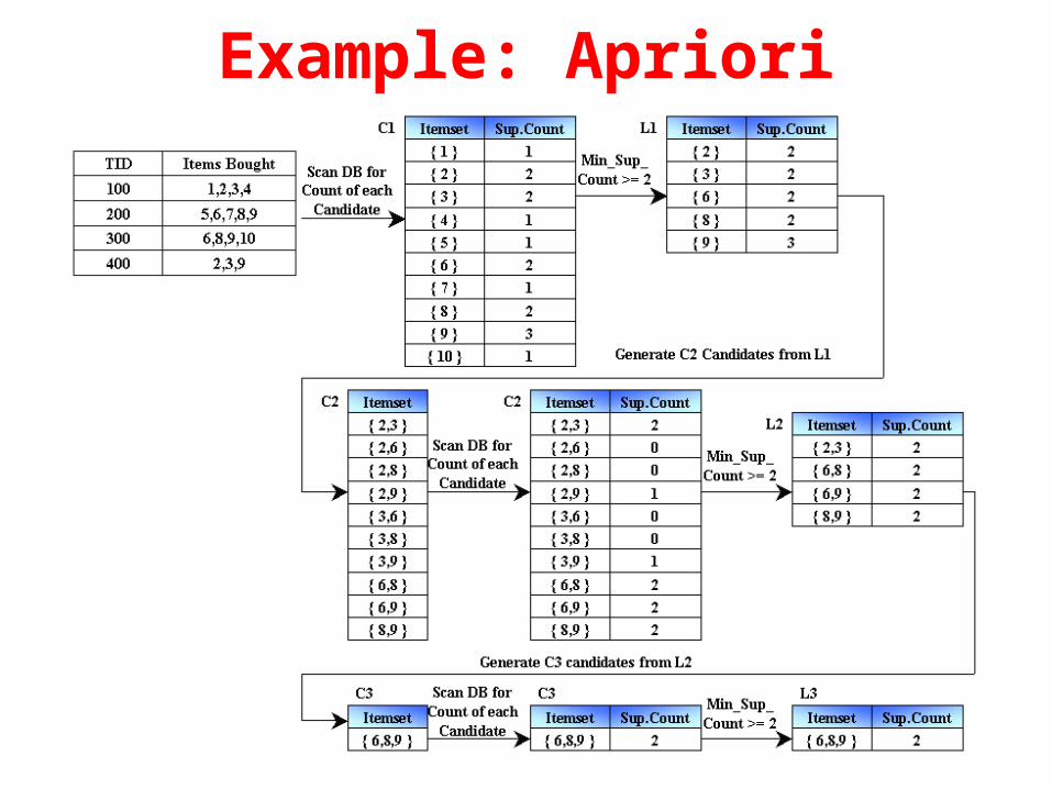
Example: Apriori
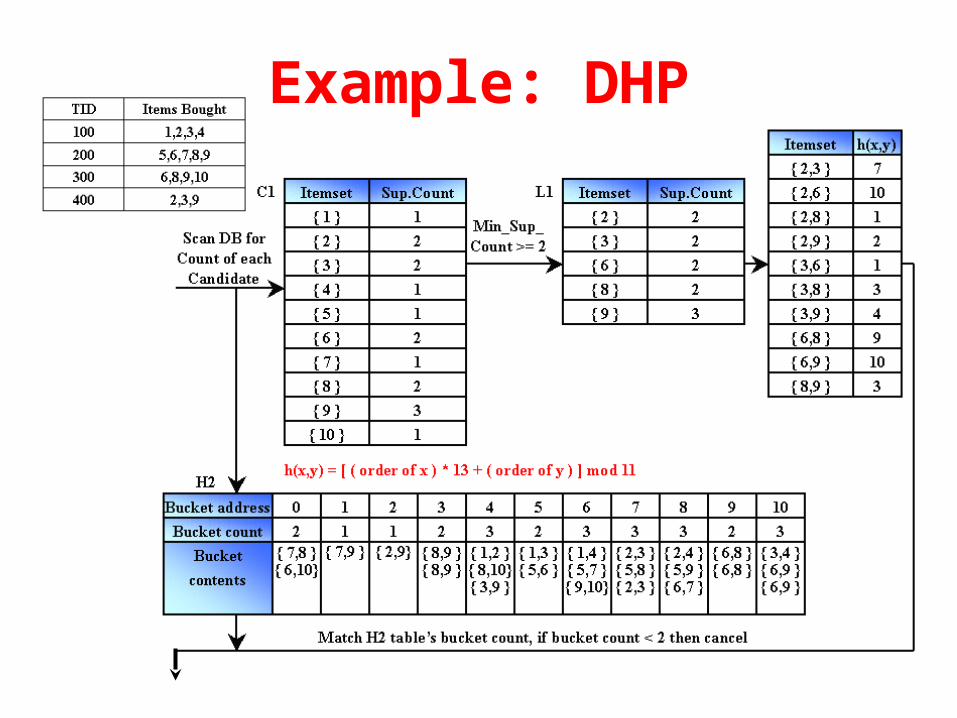
Example: DHP
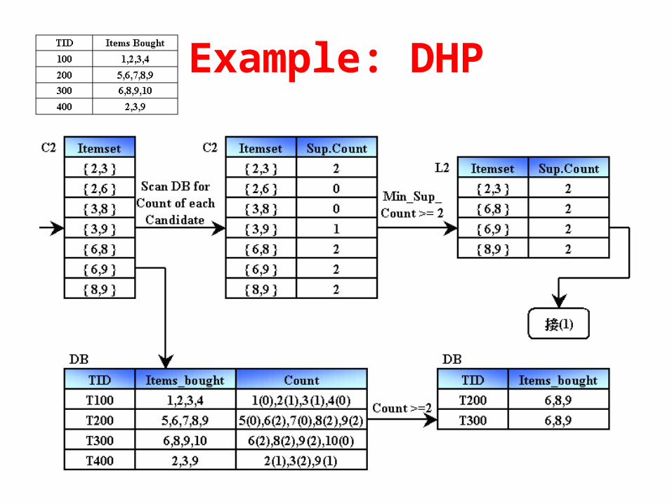
Example: DHP

Example: DHP

Mining Frequent Patterns Without Candidate Generation
• Compress a large database into a compact, Frequent-Pattern tree (FP-tree) structure– highly condensed, but complete for frequent pattern mining
– avoid costly database scans
• Develop an efficient, FP-tree-based frequent pattern mining method– A divide-and-conquer methodology: decompose mining
tasks into smaller ones
– Avoid candidate generation & sub-database test only!

Construct FP-tree from a Transaction DB
Construction Steps
• Scan DB once, find frequent 1-itemset (single item pattern)
• Order frequent items in frequency descending order
• Sorting DB according to the frequency descending order
• Scan DB again, construct FP-tree

Benefits of the FP-Tree Structure
• Completeness– never breaks a long pattern of any transaction– preserves complete information for frequent pattern
mining
• Compactness– reduce irrelevant information—infrequent items are
gone– frequency descending ordering: more frequent items
are more likely to be shared– never be larger than the original database (if not count
node-links and counts)– Compression ratio could be over 100

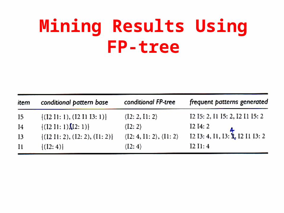
Frequent Pattern Growth
• For I5– {I1, I5}, {I2, I5}, {I2, I1, I5}
• For I4– {I2, I4}
• For I3– {I1, I3}, {I2, I3}, {I2, I1, I3}
• For I1– {I2, I1}
Order frequent items in frequency descending order

Frequent Pattern Growth• For I5
– {I1, I5}, {I2, I5}, {I2, I1, I5}
• For I4– {I2, I4}
• For I3– {I1, I3}, {I2, I3}, {I2, I1, I3}
• For I1– {I2, I1}
SubDB
SubDB
SubDB
SubDB
TrimmingDatabases
FP-tree
Conditional FP-tree from Conditional Pattern-Base
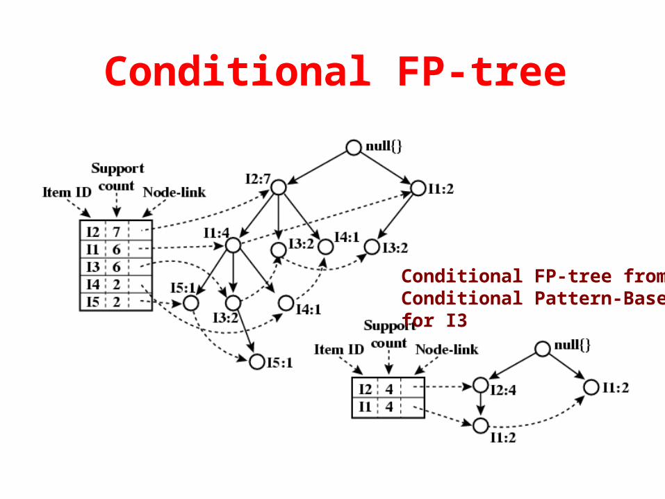
Conditional FP-tree
Conditional FP-tree fromConditional Pattern-Basefor I3

Mining Results Using FP-tree
• For I5 (不產生 NULL)– Conditional Pattern Base
• {(I2I1:1), (I2I1I3:1)}
– Conditional FP-tree
– Generate Frequent Itemsets• I2:2 Rule: I2I5:2
• I1:2 Rule: I1I5:2
• I2I1:2 Rule: I2I1I5:2
Item ID
Support
count
Node
Link
I2 2
I1 2
◎ “I2”: 2
◎ “I1”: 2
◎ NULL: 2

Mining Results Using FP-tree
• For I4
– Conditional Pattern Base• {(I2I1:1), (I2:1)}
– Conditional FP-tree
– Generate Frequent Itemsets• I2:2 Rule: I2I4:2
Item ID
Support
count
Node
Link
I2 2 ◎ “I2”: 2
◎ NULL: 2

Mining Results Using FP-tree
• For I3
– Conditional Pattern Base• {(I2I1:2), (I2:2), (I1:2)}
– Conditional FP-tree
Item ID
Support
count
Node
Link
I2 4
I1 4
◎ “I2”: 4
◎ “I1”: 2
◎ NULL: 4
◎ “I1”: 2
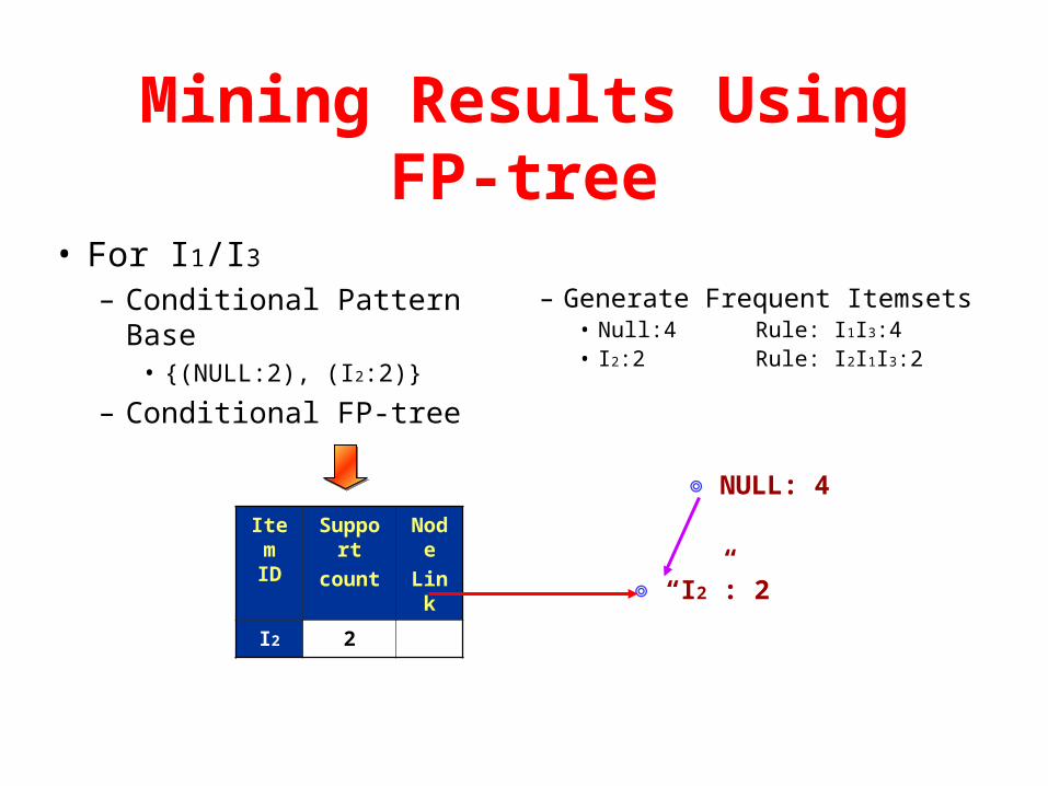
Mining Results Using FP-tree
• For I1/I3
– Conditional Pattern Base• {(NULL:2), (I2:2)}
– Conditional FP-tree
Item ID
Support
count
Node
Link
I2 2 ◎ “I2”: 2
◎ NULL: 4
– Generate Frequent Itemsets• Null:4 Rule: I1I3:4• I2:2 Rule:
I2I1I3:2

Mining Results Using FP-tree
• For I2/I3
– Conditional Pattern Base• {(NULL:4)}
– Conditional FP-tree
◎ NULL: 4
– Generate Frequent Itemsets• Null Rule: I2I3:4

Mining Results Using FP-tree
• For I1
– Conditional Pattern Base• {(NULL:2), (I2:4)}
– Conditional FP-tree
– Generate Frequent Itemsets• I2:4 Rule: I2I1:4
Item ID
Support
count
Node
Link
I2 4 ◎ “I2”: 4
◎ NULL: 6
Mining Results Using FP-tree

Mining Frequent PatternsUsing FP-tree
• General idea (divide-and-conquer)– Recursively grow frequent pattern path using the FP-tree
• Method – For each item, construct its conditional pattern-base, and
then its conditional FP-tree
– Repeat the process on each newly created conditional FP-tree
– Until the resulting FP-tree is empty, or it contains only one path (single path will generate all the combinations of its sub-paths, each of which is a frequent pattern)

Major Steps to Mine FP-tree
• Construct conditional pattern base for each
item in the FP-tree
• Construct conditional FP-tree from each
conditional pattern-base
• Recursively mine conditional FP-trees and
grow frequent patterns obtained so far If the conditional FP-tree contains a single path,
simply enumerate all the patterns
Virtual Items in Association Mining• Different region exhibit different selling patterns. Thus,
including as virtual item the information on the location or the type of stores (existing or new) where the purchase was made will enable the comparisons between locations or types within a single chain
• Virtual item may include information on whether the purchase was made with cash, a credit card or check. The inclusion of such virtual item allows to analyze the association between the payment method and items purchased.
• Virtual item may include information on the day of the week or the time of the day the transaction occurred. The inclusion of such virtual item allows to analyze the association between the transaction time and items purchased
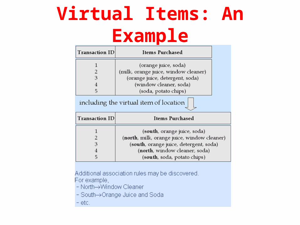
Virtual Items: An Example
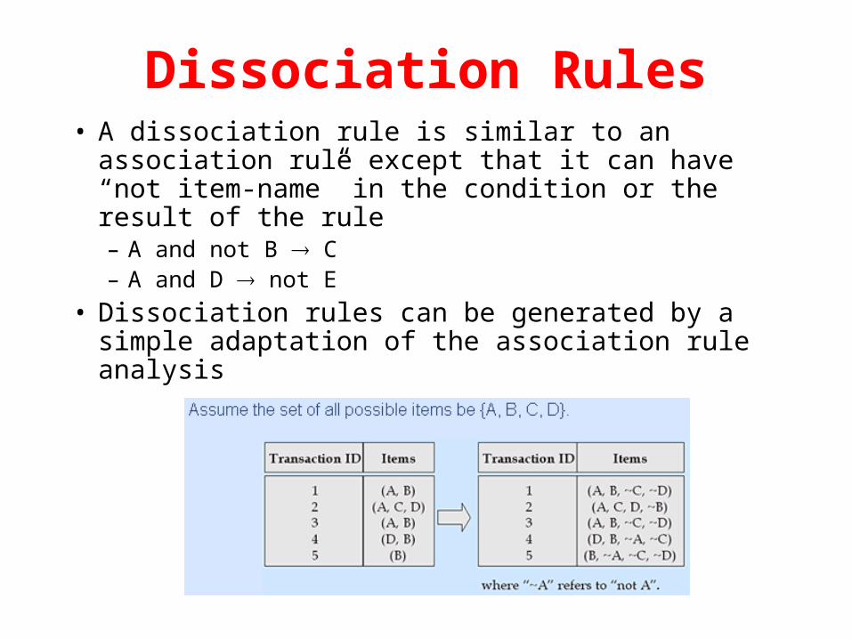
Dissociation Rules• A dissociation rule is similar to an association rule
except that it can have “not item-name” in the condition or the result of the rule– A and not B C – A and D not E
• Dissociation rules can be generated by a simple adaptation of the association rule analysis
Discussions• The size of a typical transaction grows because it now
includes inverted items• The total number of items used in the analysis doubles
– Since the amount of computation grows exponentially with the number of items, doubling the number of items seriously degrades performance
• The frequency of the inverted items tends to be much larger than the frequency of the original items. So, it tends to produce rules in which all items are inverted. These rules are less likely to be actionable. – not A and not B not C
• It is useful to invert only the most frequent items in the set used for analysis. It is also useful to invert some items whose inverses are of interest.

Interestingness Measurements
• Subjective Measures – A rule (pattern) is interesting if
• it is unexpected (surprising to the user)
• actionable (the user can do something with it)
• Objective Measures– Two popular measurements:
• Support
• confidence

Criticism to Support and Confidence
• Example 1– Among 5000 students
• 3000 play basketball• 3750 eat cereal• 2000 both play basket ball and eat cereal
– play basketball eat cereal [40%, 66.7%] is misleading because the overall percentage of students eating cereal is 75% which is higher than 66.7%.
basketball not basketball sum (row)cereal 2000 1750 3750
not cereal 1000 250 1250sum (col.) 3000 2000 5000
Criticism to Support and Confidence
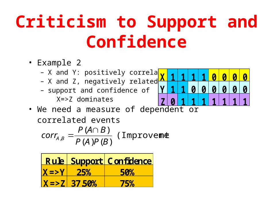
• Example 2– X and Y: positively correlated,– X and Z, negatively related– support and confidence of X=>Z dominates
• We need a measure of dependent or correlated events
X 1 1 1 1 0 0 0 0Y 1 1 0 0 0 0 0 0Z 0 1 1 1 1 1 1 1
nt)(Improveme )()(
)(, BPAP
BAPcorr BA
Rule Support ConfidenceX=>Y 25% 50%X=>Z 37.50% 75%

Criticism to Support and Confidence
• Improvement (Correlation)– Taking both P(A) and P(B) in consideration
– P(A^B)=P(B)*P(A), if A and B are independent events
– A and B negatively correlated, if the value is less than 1
otherwise A and B positively correlated
– When improvement is less than 1, negating the result produces a better
rule
• X => NOT Z
X 1 1 1 1 0 0 0 0Y 1 1 0 0 0 0 0 0Z 0 1 1 1 1 1 1 1
)()(
)(, BPAP
BAPcorr BA
Itemset Support ImprovementX,Y 25% 2X,Z 37.50% 0.9Y,Z 12.50% 0.57
Multiple-Level Association Rules
• Items often form hierarchy• Items at the lower level are expected to
have lower support• Rules regarding itemsets at appropriate
levels could be quite useful• Transaction database can be encoded based
on dimensions and levels• We can explore multi-level mining
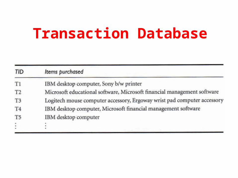
Transaction Database

Concept Hierarchy

Mining Multi-Level Associations
• A top_down, progressive deepening approach– First find high-level strong rules
milk bread [20%, 60%]
– Then find their lower-level “weaker” rules2% milk wheat bread [6%, 50%]
• Variations at mining multiple-level association rules.– Cross-level association rules (Generalized Asso. Rules)
2% milk Wonder wheat bread
– Association rules with multiple, alternative hierarchies2% milk Wonder bread

Multi-level Association: Uniform Support vs. Reduced Support
• Uniform Support: the same minimum support for all levels– One minimum support threshold is needed.– Lower level items do not occur as frequently. If support threshold
• too high miss low level associations• too low generate too many high level associations
• Reduced Support: reduced minimum support at lower levels– There are 4 search strategies:
• Level-by-level independent• Level-cross filtering by k-itemset• Level-cross filtering by single item• Controlled level-cross filtering by single item
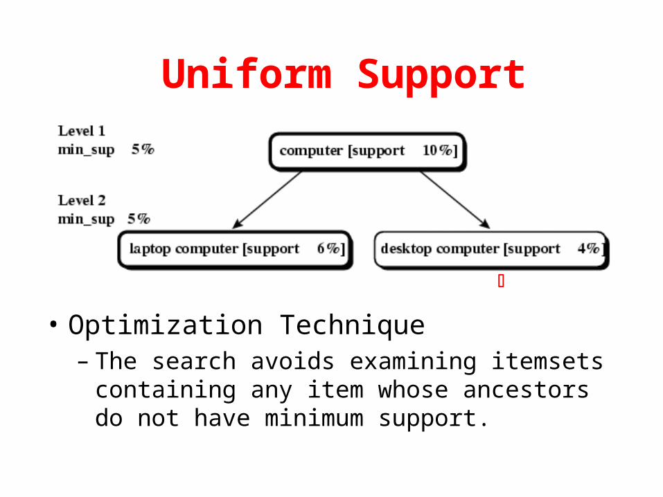
Uniform Support
• Optimization Technique– The search avoids examining itemsets containing
any item whose ancestors do not have minimum support.
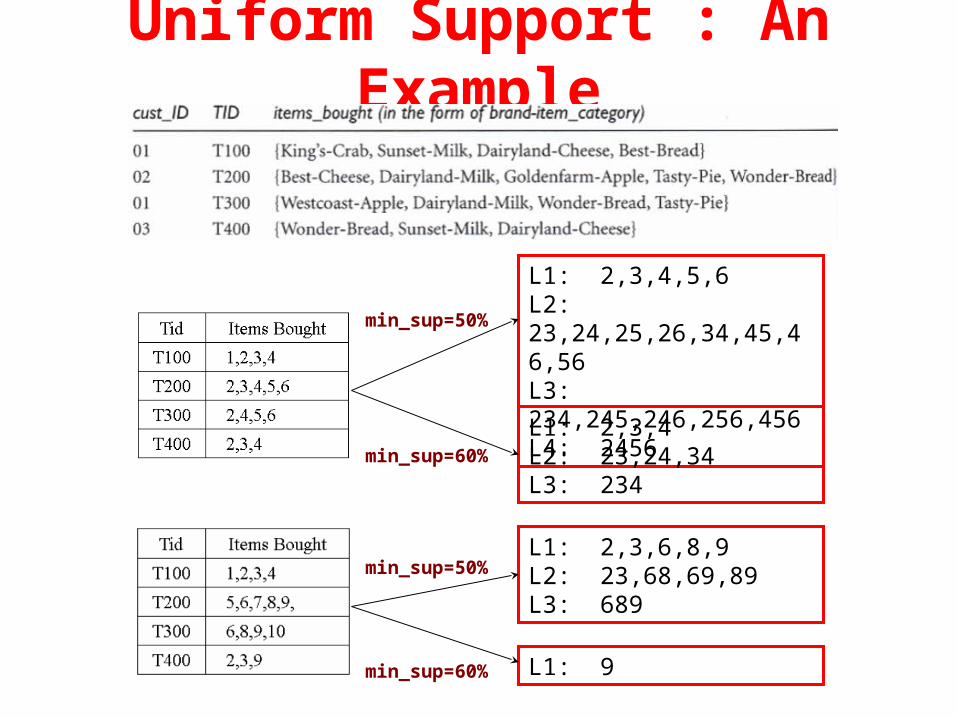
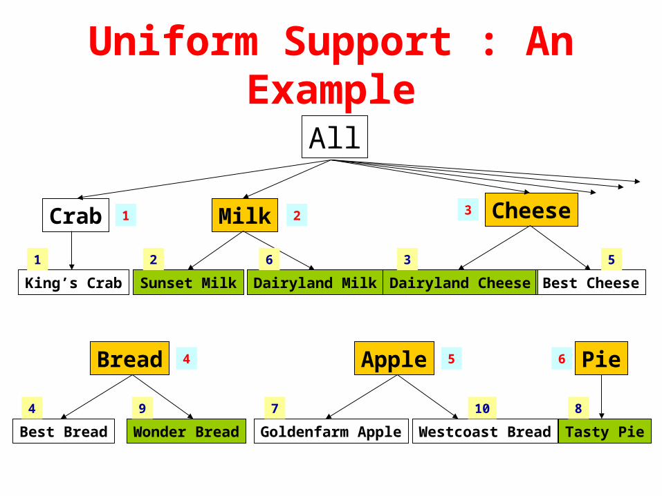
Uniform Support : An Example
L1: 2,3,4,5,6L2: 23,24,25,26,34,45,46,56L3: 234,245,246,256,456L4: 2456
L1: 2,3,6,8,9L2: 23,68,69,89L3: 689
L1: 2,3,4L2: 23,24,34L3: 234
L1: 9
min_sup=50%
min_sup=60%
min_sup=50%
min_sup=60%
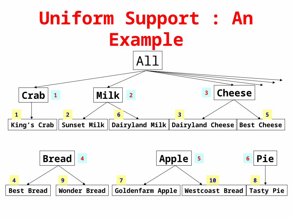
Uniform Support : An Example
Crab
King’s Crab Sunset Milk Dairyland Milk Dairyland Cheese Best Cheese
Milk Cheese
All
Best Bread Wonder Bread
Bread
Goldenfarm Apple Westcoast Bread
Apple Pie
Tasty Pie
1 2 3
4 5 6
1 2 6 3 5
4 9 7 10 8

Uniform Support : An Example
L1: 2,3,4,5,6L2: 23,24,25,26,34,45,46,56L3: 234,245,246,256,456L4: 2456
L2: 23,68,69,89L3: 689
min_sup=50%
min_sup=50%
L1: 2,3,6,8,9min_sup=50%
C2: 23,36,29,69,28,68,39,89C3: 239,369,289,689
Scan DB
Scan DB
(1) (2)
(3)
Apriori/DHPFP Growth
Uniform Support : An Example
Crab
King’s Crab Sunset Milk Dairyland Milk Dairyland Cheese Best Cheese
Milk Cheese
All
Best Bread Wonder Bread
Bread
Goldenfarm Apple Westcoast Bread
Apple Pie
Tasty Pie
1 2 3
4 5 6
1 2 6 3 5
4 9 7 10 8

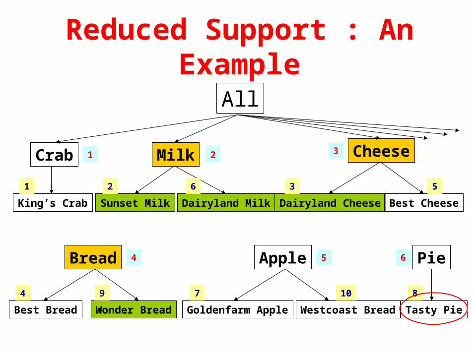
Reduced Support
• Each level of abstraction has its own minimum support threshold.
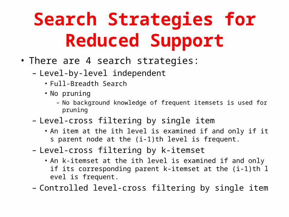
Search Strategies forReduced Support
• There are 4 search strategies:– Level-by-level independent
• Full-Breadth Search
• No pruning– No background knowledge of frequent itemsets is used for pruning
– Level-cross filtering by single item• An item at the ith level is examined if and only if its parent node
at the (i-1)th level is frequent.
– Level-cross filtering by k-itemset• An k-itemset at the ith level is examined if and only if its corresp
onding parent k-itemset at the (i-1)th level is frequent.
– Controlled level-cross filtering by single item

Level-Cross Filtering by Single Item
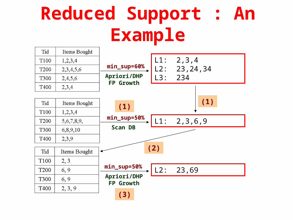
Reduced Support : An Example
L2: 23,69
min_sup=60%
min_sup=50%
L1: 2,3,6,9min_sup=50%
Scan DB
Apriori/DHPFP Growth
(1)
(2)
(3)
(1)
L1: 2,3,4L2: 23,24,34L3: 234Apriori/DHP
FP Growth

Reduced Support : An Example
Crab
King’s Crab Sunset Milk Dairyland Milk Dairyland Cheese Best Cheese
Milk Cheese
All
Best Bread Wonder Bread
Bread
Goldenfarm Apple Westcoast Bread
Apple Pie
Tasty Pie
1 2 3
4 5 6
1 2 6 3 5
4 9 7 10 8

Level-Cross Filtering by K-Itemset
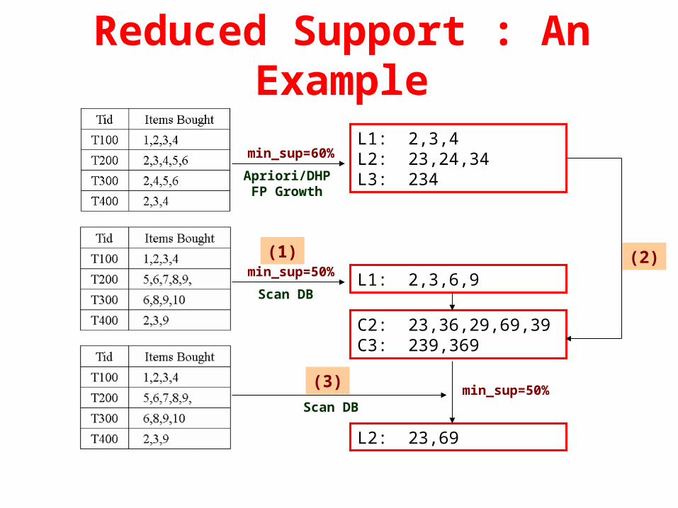
Reduced Support : An Example
L2: 23,69
min_sup=60%
min_sup=50%
L1: 2,3,6,9min_sup=50%
C2: 23,36,29,69,39C3: 239,369
Scan DB
Scan DB
(1) (2)
(3)
Apriori/DHPFP Growth
L1: 2,3,4L2: 23,24,34L3: 234
Reduced Support : An Example
Crab
King’s Crab Sunset Milk Dairyland Milk Dairyland Cheese Best Cheese
Milk Cheese
All
Best Bread Wonder Bread
Bread
Goldenfarm Apple Westcoast Bread
Apple Pie
Tasty Pie
1 2 3
4 5 6
1 2 6 3 5
4 9 7 10 8

Reduced Support• Level-by-level independent
– It is very relaxed in that it may lead to examining numerous infrequent items at low levels, finding associations between items of little importance.
• Level-cross filtering by k-itemset– It allows the mining system to examine only the children of frequent
k-itemsets.– This restriction is very strong in that there usually are not many k-
itemsets.– Many valuable patterns may be filtered out.
• Level-cross filtering by single item– A compromise between the above two approaches– This method may miss associations between low level items that are
frequent based on a reduced minimum support, but whose ancestors do not satisfy minimum support.
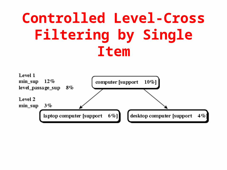
Controlled Level-Cross Filtering by Single Item

Reduced Support : An Example
min_sup=60%
min_sup=50%
L1: 2,3,6,8,9min_sup=50%
Scan DB
Apriori/DHPFP Growth
(1)
(2)
(3)
(1)
L1: 2,3,4L2: 23,24,34L3: 234Apriori/DHP
FP Growth
level_passage_sup=50%L1: 2,3,4,5,6
L2: 23,68,69,89L3: 689

Reduced Support : An Example
Crab
King’s Crab Sunset Milk Dairyland Milk Dairyland Cheese Best Cheese
Milk Cheese
All
Best Bread Wonder Bread
Bread
Goldenfarm Apple Westcoast Bread
Apple Pie
Tasty Pie
1 2 3
4 5 6
1 2 6 3 5
4 9 7 10 8
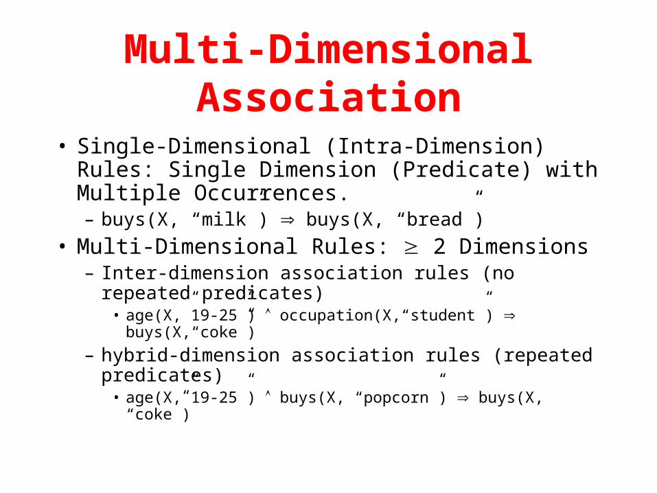
Multi-Dimensional Association
• Single-Dimensional (Intra-Dimension) Rules: Single Dimension (Predicate) with Multiple Occurrences.– buys(X, “milk”) buys(X, “bread”)
• Multi-Dimensional Rules: 2 Dimensions– Inter-dimension association rules (no repeated
predicates)• age(X,”19-25”) occupation(X,“student”) buys(X,“coke”)
– hybrid-dimension association rules (repeated predicates)
• age(X,”19-25”) buys(X, “popcorn”) buys(X, “coke”)

Summary• Association rule mining
– Probably the most significant contribution from the database community in KDD
– A large number of papers have been published
• Some Important Issues– Generalized Association Rules
– Multiple-Level Association Rules
– Association Analysis in Other Types of Data• Spatial Data, Multimedia Data, Time Series Data, etc.
– Weighted Association Rules
– Quantitative Association Rules

Weighted Association Rules
• Why Weighted Association Analysis? – In previous work, all items in a transactional database
are treated uniformly
– Items are given weights to reflect their importance to the user
– The weights may correspond to special promotions on some products, or the profitability of different items
• Some products may be under promotion and hence are more interesting, or some products are more profitable and hence rules concerning them are of greater values
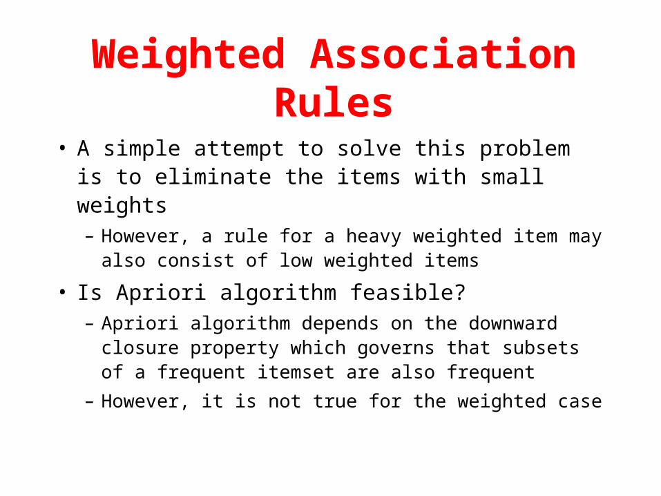
Weighted Association Rules
• A simple attempt to solve this problem is to eliminate the items with small weights– However, a rule for a heavy weighted item may also
consist of low weighted items
• Is Apriori algorithm feasible?– Apriori algorithm depends on the downward closure
property which governs that subsets of a frequent itemset are also frequent
– However, it is not true for the weighted case

Weighted Association Rules:An Example
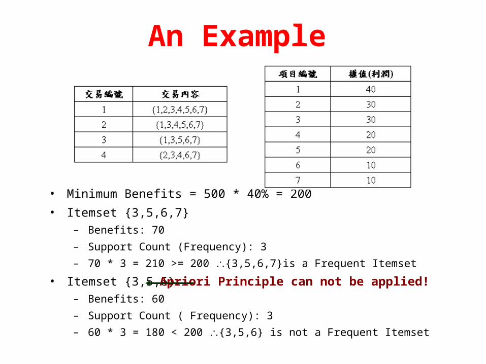
• Total Benefits: 500– Benefits for the First Transaction: (40+30+30+20+20+10+ 10)=160
– Benefits for the Second Transaction: (40+30+20+ 20+10+10)=130
– Benefits for the Third Transaction: (40+30+20+10+10)= 110
– Benefits for the Fourth Transaction: (30+30+20+10+10)=100
• Suppose Weighted_Min_Sup = 40%– Minimum Benefits = 500 * 40% = 200
An Example
• Minimum Benefits = 500 * 40% = 200
• Itemset {3,5,6,7}– Benefits: 70
– Support Count (Frequency): 3
– 70 * 3 = 210 >= 200 {3,5,6,7}is a Frequent Itemset
• Itemset {3,5,6}– Benefits: 60
– Support Count ( Frequency): 3
– 60 * 3 = 180 < 200 {3,5,6} is not a Frequent Itemset
Apriori Principle can not be applied!

K-Support Bound• If Y is a frequent q-itemset
– Support_Count(Y) (Weighted_Min_Sup * Total_Benefits) / Benefits(Y)
• Example– {3,5,6,7} is a Frequent 4-Itemset
• Support_Count({3,5,6,7}) = 3 (40% * 500) / Benefits({3,5,6,7}) = (40% * 500) / 70 = 2.857
• If X is a frequent k-itemset containing q-itemset Y– Minimum_Support_Count(X)
(Weighted_Min_Sup * Total_Benefits) / (Benefits(Y) + (k-q) Maximum Remaining Weights)
• Example– X is a Frequent 5-Itemset containing {3,5,6,7}
• Minimum_Support_Count(X) (40% * 500) / (70 + 40) = 1.81
K-Support Bound
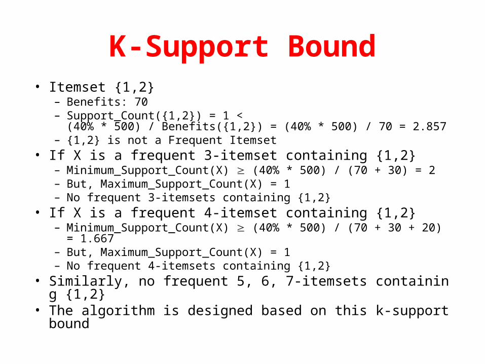
K-Support Bound• Itemset {1,2}
– Benefits: 70– Support_Count({1,2}) = 1 <
(40% * 500) / Benefits({1,2}) = (40% * 500) / 70 = 2.857– {1,2} is not a Frequent Itemset
• If X is a frequent 3-itemset containing {1,2}– Minimum_Support_Count(X) (40% * 500) / (70 + 30) = 2– But, Maximum_Support_Count(X) = 1– No frequent 3-itemsets containing {1,2}
• If X is a frequent 4-itemset containing {1,2}– Minimum_Support_Count(X) (40% * 500) / (70 + 30 + 20) = 1.667– But, Maximum_Support_Count(X) = 1– No frequent 4-itemsets containing {1,2}
• Similarly, no frequent 5, 6, 7-itemsets containing {1,2}• The algorithm is designed based on this k-support bound

MINWAL Algorithm

Step by Step
• Input: Product & Transactional Databases
Total Profits: 1380
Weighted_Min_Sup = 50%

Step 2, 7
• Search(D)– This subroutine finds out the maximum transaction size in
that transactional database D• Size = 4 in this case
• Counting(D, w)– This subroutine cumulates the support counts of the 1-ite
msets– The k-support bounds of each 1-itemset will be calculated,
and the 1-itemsets with support counts greater than any of the k-support bounds will be kept in C1

Step 7
K-Support Bound (50% * 1380) / (10 + 90) = 6.9
Step 11
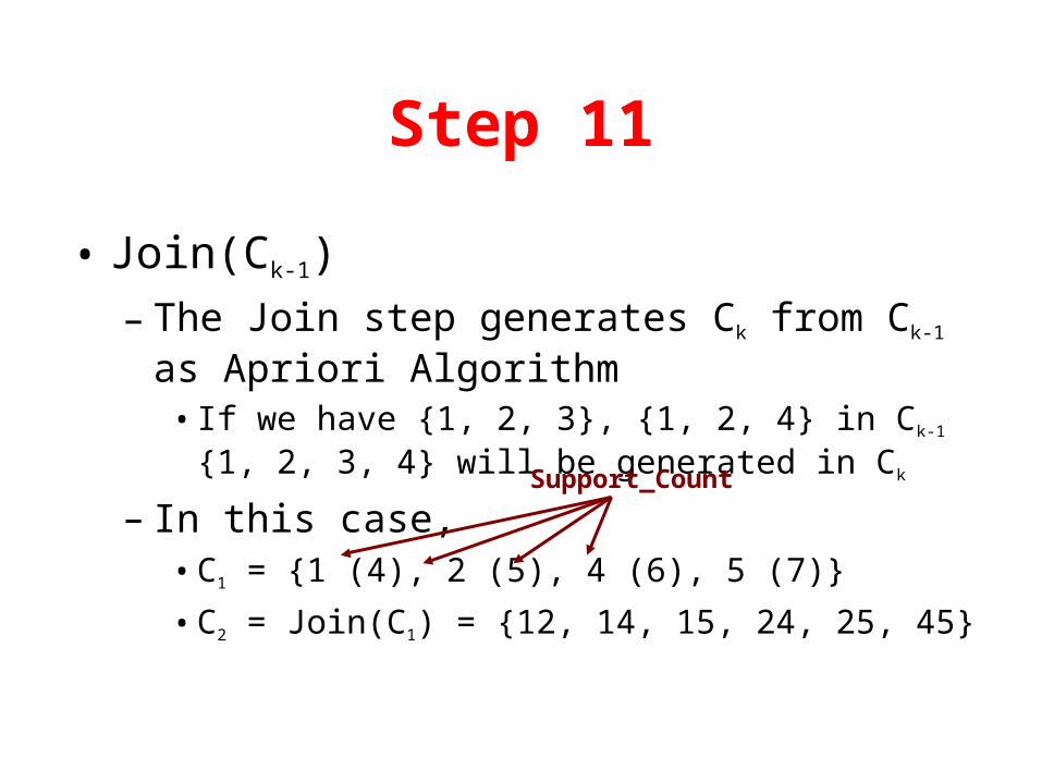
• Join(Ck-1)
– The Join step generates Ck from Ck-1 as Apriori Algorithm
• If we have {1, 2, 3}, {1, 2, 4} in Ck-1 {1, 2, 3, 4} will be generated in Ck
– In this case,• C1 = {1 (4), 2 (5), 4 (6), 5 (7)}
• C2 = Join(C1) = {12, 14, 15, 24, 25, 45}
Support_Count

Step 12• Prune(Ck)
– The itemset will be pruned in either of the following cases• A subset of the candidate itemset in Ck does not exist in Ck-1
• Estimate an upper bound on the support count (SC) of the joined itemset X, which is the minimum support count among the k different (k-1)-subsets of X in Ck-1. If the estimated upper bound on the support count shows that the itemset X cannot be a subset of any large itemset in the coming passes (from the calculation of k-support bounds for all itemsets), that itemset will be pruned
– In this case,• C2 = Prune(C2) = {12 (4), 14 (4), 15 (4), 24 (5), 25 (5), 45 (6)}
• Using K-Support-Bound
Estimated_Support_Count

Step 12• Prune(Ck)
– Using K-Support-Bound (No one is pruned)
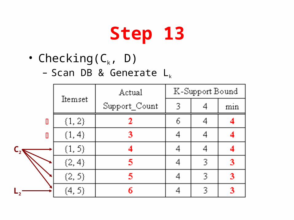
Step 13• Checking(Ck, D)
– Scan DB & Generate Lk
L2
C2
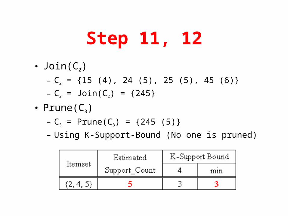
Step 11, 12
• Join(C2)– C2 = {15 (4), 24 (5), 25 (5), 45 (6)}
– C3 = Join(C2) = {245}
• Prune(C3)– C3 = Prune(C3) = {245 (5)}
– Using K-Support-Bound (No one is pruned)

Step 13
• Checking(C3, D): Scan DB
• C3 = L3 = {245}
• Finally, L = {45, 245}
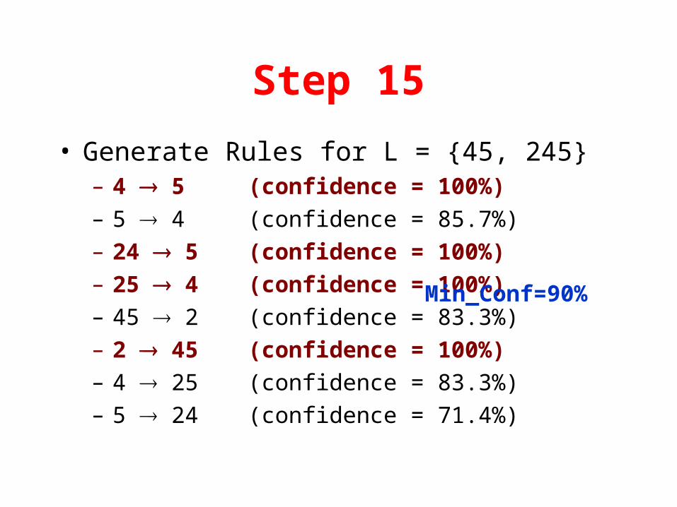
Step 15
• Generate Rules for L = {45, 245}– 4 5 (confidence = 100%)
– 5 4 (confidence = 85.7%)
– 24 5 (confidence = 100%)
– 25 4 (confidence = 100%)
– 45 2 (confidence = 83.3%)
– 2 45 (confidence = 100%)
– 4 25 (confidence = 83.3%)
– 5 24 (confidence = 71.4%)
Min_Conf=90%
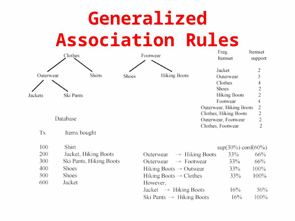
Generalized Association Rules
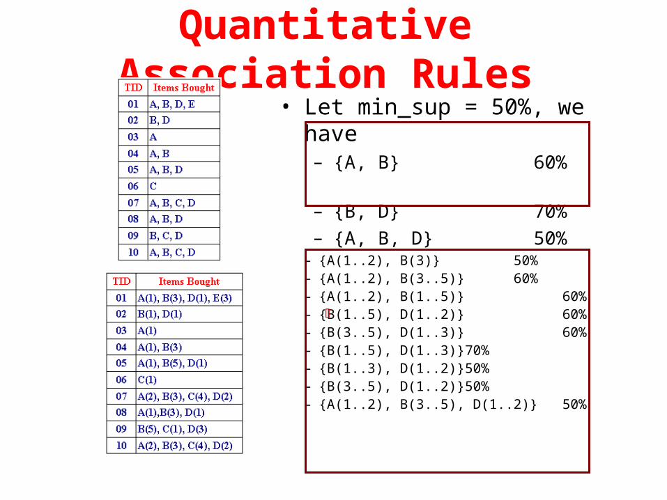
Quantitative Association Rules
– {A(1..2), B(3)} 50%– {A(1..2), B(3..5)} 60%– {A(1..2), B(1..5)} 60%– {B(1..5), D(1..2)} 60%– {B(3..5), D(1..3)} 60%– {B(1..5), D(1..3)} 70%– {B(1..3), D(1..2)} 50%– {B(3..5), D(1..2)} 50%– {A(1..2), B(3..5), D(1..2)} 50%
• Let min_sup = 50%, we have– {A, B} 60%
– {B, D} 70%
– {A, B, D} 50%