minicourse on femlab

Minicourse on FEMLAB

This minicourse is an introduction to working with FEMsolution of a large class of partial differential equations (physics. The program has been written in a way that makengineer who is unaccustomed to PDE´s, as well a

The object of the course is to present three examplusing FEMLAB modeling. If you are new to FEMLAstart with exercise 1.

You need to download comp.dxf. Also, answers to files eldet.m,comp.m and difflow.m

ContentsFEMLAB

FEMLAB Structural Mechanics

FEMLAB Electromagnetics

FEMLAB in Simulink

Exercise 1: An electronic Detector

Exercise 2: Mechanical Component Model

Exercise 3: Chemical Engineering

1

LAB, a program for the PDE) from different fields of es it easy to use, both for the s for the specialist in PDE´s.

es that will get the user started in B, it is recommended that you

the exercises are provided in the

FEMLAB

FEMLABFEMLAB solves Partial Differential Equations (PDE) that arise in engineering and scientific applications, using the finite element method.

Areas of physics where FEMLAB could be applied are e.g.

• electromagnetics

• heat flow

• chemistry

• diffusion

• fluid mechanics

• structural mechanics

• general physics

• wave propagation

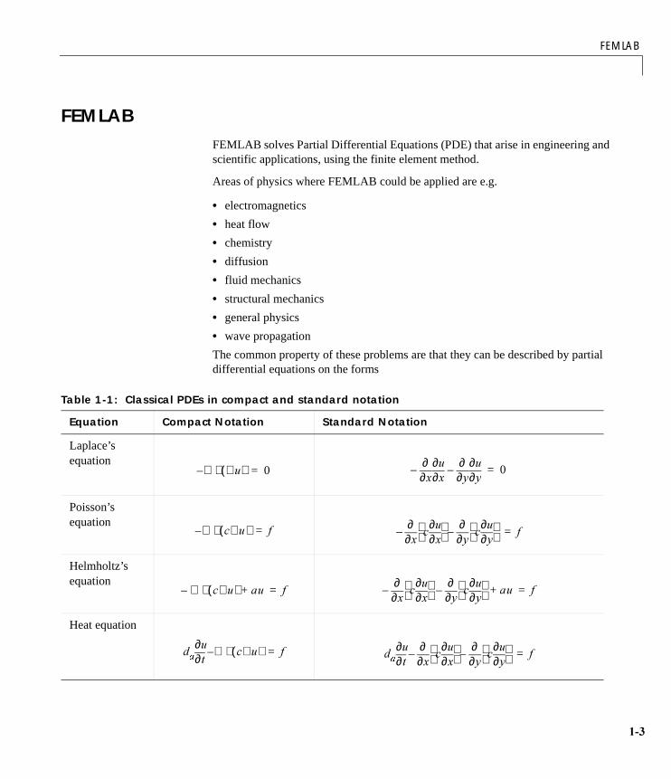
The common property of these problems are that they can be described by partial differential equations on the forms

Table 1-1: Classical PDEs in compact and standard notation

Equation Compact Notation Standard Notation

Laplace’s equation

Poisson’s equation

Helmholtz’s equation

Heat equation

∇ X∇( )⋅– 0=[∂

∂[∂

∂X–

\∂∂

\∂∂X

– 0=

∇ F X∇( )⋅– I=[∂

∂F

[∂∂X

\∂∂

F\∂

∂X –– I=

∇ F X∇( )⋅– DX+ I=[∂

∂F

[∂∂X

\∂∂

F\∂

∂X –– DX+ I=

GD W∂∂X ∇ F X∇( )⋅– I= GD W∂

∂X[∂

∂ F[∂

∂X

\∂∂ F

\∂∂X

–– I=

1

s of and inner

the n of

cial

e set ics

uited

These PDE´s are solved in two dimensions. The boundary conditions on edgedomains are prescribed values of the solution and its derivatives, i. e. DirichletGeneralized Neumann conditions. Boundary conditions can also be applied to edges. An additional feature is the possibility to specify periodic boundary conditions.

To facilitate for the user, different physics modes have been created. In thesePDE and the boundary conditions are formulated in a way that is customary indifferent scientific areas. There are still modes for the mathematical formulatioPDE´s.

It is possible to solve coupled systems of PDE´s. Actually, FEMLAB has a spefeature to make this easy and intuitive, which is called PXOWLSK\VLFV. Using this, different modes can be added in the GUI and FEMLAB automatically sets up thof coupled PDE´s. In the third exercise you will learn how to use the multiphysfeature to set up a coupled system of PDE.

Most problems are solved in a way, where the basic PDE´s are put on a form, sfor linear or almost linear problems. We call this the FRHIILFLHQWIRUP. For strongly non-linear PDE´s, however, it is better to use a formulation, called the JHQHUDOIRUP. You will encounter this latter formulation in the last exercise.

Wave equation

Schrödinger equation

Convection- reaction equation

Table 1-1: Classical PDEs in compact and standard notation

Equation Compact Notation Standard Notation

GDW2

2

∂

∂ X ∇ F X∇( )⋅– I= GDW2

2

∂

∂ X[∂

∂F

[∂∂X

\∂∂

F\∂

∂X –– I=

∇ F X∇( )⋅– DX+ λX= [∂∂ F

[∂∂X

\∂∂ F

\∂∂X

–– DX+ λX=

GD W∂∂X ∇ F X∇( )⋅– β X∇⋅+ I= GD W∂

∂X[∂

∂F

[∂∂X

\∂∂

F\∂

∂X –– +

β[ [∂∂X β\ \∂

∂X+ I=

FEMLAB

des,

The finite element mesh is generated using a Delaunay algorithm in order to ensure compatibility with the geometry, while still keeping the finite element angles as large as possible. This increases accuracy and the speed of the adaptive solver. You can control the parameter of the mesh directly. Adjustable parameter are e.g. the global element size and the element size on an edge.

Using the adaptive mesh solver, the mesh is refined during the solution in areas where some error estimate is too large. The different solvers can handle linear, nonlinear, as well as eigenfrequency problems.

The logic of modelling in FEMLAB follows the natural steps for solving PDE´s,using the finite element method.

• Draw the domain geometry

• Specify boundary conditions

• Define the PDE´s, either by specifying physical parameters in the physics moor by inserting coefficients in mathematical PDE formulations.

• Generate a mesh

• Discretize the equations and solve on the mesh.

In the Graphical User Interface (GUI), FEMLAB lets you navigate easily back and forth among these steps. A set of CAD tools are provided to draw the geometry of the model, and a set of postprocessing functions offer a wide range of possibilities to analyze the results. Apart from plotting the results over the geometry, data can be obtained along curves. Integrals, both over the geometry and along lines, can also be computed.You will get acquainted to modeling in the GUI by doing the exercises below.

When modeling in the GUI, it is still possible to use matlab functions, by inserting their names in e.g. the fields for the specification of PDE coefficients.

It is also possible to use FEMLAB directly in the Matlab environment, using the special FEMLAB commands. This is not covered in this minicourse. But if you save your model as an m-file, you can see the different commands used for creating and solving the model. Command line modelling allows the user to do parameter studies on their model as Matlab programs. The $3,, furthermore, makes it possible for the user to customize the GUI, to incorporate this parameter study. For all this, we refer to the FEMLAB manuals

1

FEMLAB Structural MechanicsStructural mechanics can be modeled in the basic FEMLAB program. FEMLAB Structural Mechanics1, however, extends the capability of FEMLAB in this area. It provides several additional features of importance. Application modes are

• Plane stress problems

• Plane strain problems

• Axial symmetric problems

• Kirchhoff plate problems

• Mindlin plate problems

The first three types of application modes are basically two-dimensional. All displacements and loads are in the geometrical plane. The two plate modes, on the other hand, allows for the specification of some three-dimensional properties in a two-dimensional model. For these modes, it is possible to specify torsion and load directed out of the plane.

For the above modes, the models can be static or time-dependent. Analysis of eigenfrequency and frequency response can be made, using the corresponding solvers.

Bars and beams can be modeled together with two-dimensional objects in the plane stress mode and in the plate modes. A beam type element is a combination of a bending element and a bar element.

To create a beam, draw a straight line in the 'UDZ mode and then open the 6SHFLI\(OHPHQWdialog box, in the (OHPHQWV menu. Check the (GJHV radio button and select the appropriate beam element type. In the example below, a beam is to be attached to a rectangle. By default, the beam is fixed to another geometry object.

1. In the navigator, denoted Structural Mechanics Module.


However, you can disconnect one or several degrees of freedom, using the 'LVFRQQHFW(GJHV dialog box, also found in the (OHPHQWVmenu.

1

For the two-dimensional subdomain, you can specify different types of finite elements. Higher order elements, like 8-node quadrilaterals and 6-node triangles are available.

In FEMLAB Structural Mechanics you can use a local coordinate system when setting loads and constraints


Using this property, it is easy to set a normal load on an edge with a complex shape.

Other valuable properties of FEMLAB Structural Mechanics are

• The material library

• The possibility of specifying models with plasticity

• The possibility of modeling dynamic problems with damping.

1

FEMLAB ElectromagneticsFEMLAB Electromagnetics2 is a collection of application modes, customized for engineers and physicists working within the field of electromagnetics.

The types of problem that can be solved, can be classified into

• In-plane quasi-statics

• Axisymmetric quasi-static

• In-plane waves

• Axisymmetric waves

• Perpendicular waves

For these problems, static, time-harmonic and time-dependent models can be specified.

Of the above, the first two types use similar approaches for simulating electromagnetic phenomena. They only differ in the coordinate system used for describing the geometric structures. In the same manner the last three types form a group with common simulation strategies. The last type describes 3-D problems with a harmonic propagation in one direction. These can be simplified to 2-D simulations.

The difference between the two groups is that the design of the modes depend on the HOHFWULFDOVL]H of the structure. The electrical size is a dimension-less measure given as the ratio between the largest distance between two points in the structure divided by the wavelength of the electromagnetic fields. This distinction is based on whether the retarded field3 has to be taken into account or not. The latter case is often referred to as the TXDVLVWDWLFDSSUR[LPDWLRQ.

Quasi-static modes are suitable for simulations of structures with electrical sizes of up to 1/10.

When the variations in time of the sources of the electromagnetic fields are more rapid, the full Maxwell modes have to be used. These modes are appropriate for structures of electrical size 1/100 and larger. This means that there is an overlapping range where quasi-static or full Maxwell modes can be used equally well.

For analysis of electro-mechanical devices, such as linear and rotary motors, the computation of the forces and force distribution is important. It turns out that the

2. In the navigator, denoted Electromagnetics Module.

3. Cheng, D. K. )LHOGDQG:DYH(OHFWURPDJQHWLF 1989, Addison-Wesley, Reading.

FEMLAB Electromagnetics

latter is difficult. To enable the calculation of force distribution, FEMLAB Electromagnetics has a special function, based on the principle of virtual work for magnetic energy.

FEMLAB Electromagnetics can handle

• Inhomogeneous materials

• Anisotropic materials

• Nonlinear materials

• Frequency dispersive materials.

1

FEMLAB in Simulink6LPXOLQN is a Matlab product for simulation of dynamical systems. It provides you with a graphical user interface, enabling the building of models from a number of connected blocks, each representing an operation performed on a data flow. Simulink is used, e. g., for validation of control systems, signal processing and optimization.

A FEMLAB model can be exported as a )(0/$%6LPXOLQNVWUXFWXUH. This structure provides an interface between Simulink and FEMLAB. Thus, the model can be incorporated as a block in a Simulink model.

It should always be considered, whether the FEMLAB model makes it possible to use a FEMLAB Simulink structure, that does not call FEMLAB during the simulation. Thus, a faster Simulink model can be obtained for a linear FEMLAB model, if the FEMLAB model has been exported as a VWDWHVSDFH model. Also, if the time-scale of the FEMLAB model is significantly shorter than the time scale of the Simulink model, a VWDWLF model of FEMLAB should be exported.

The input data to the FEMLAB Simulink structure is passed using variables. These variables are the ones specified in the $GG(GLW9DULDEOHV dialog box, and not the dependent variables. Simulink cannot handle dirichlet boundary conditions that depends on input variables from Simulink.

Output data can be on different forms, all derived from dependent variables.

• The solution or solution component at a given node in the mesh.

• An expression evaluated at a given node.

• A user defined Matlab function

• A linear functional of the solution

Exercise 1: An Electronic Detector

Exercise 1: An Electronic DetectorIn this example you will calculate the electric field in a part of an electronic detector. The part of the detector that we will model consists of an array of electrodes (cathodes) between two electrodes at 100 V. This is described in more detail on the web site http://hsbpc1.ikf.physik.uni-frankfurt.de/detektor/Hand1/hand1.htm. Due to the symmetry property of the problem, we will only model a domain with three electrodes.

Start FEMLAB from the Matlab command window by typing

IHPODE

The 0RGHO1DYLJDWRU now appears. If not, go to the)LOH menu and select 1HZ. Select 3K\VLFVPRGHV and double click. Then choose (OHFWURVWDWLFV and /LQHDUVWDWLRQDU\. Then press 2..

1

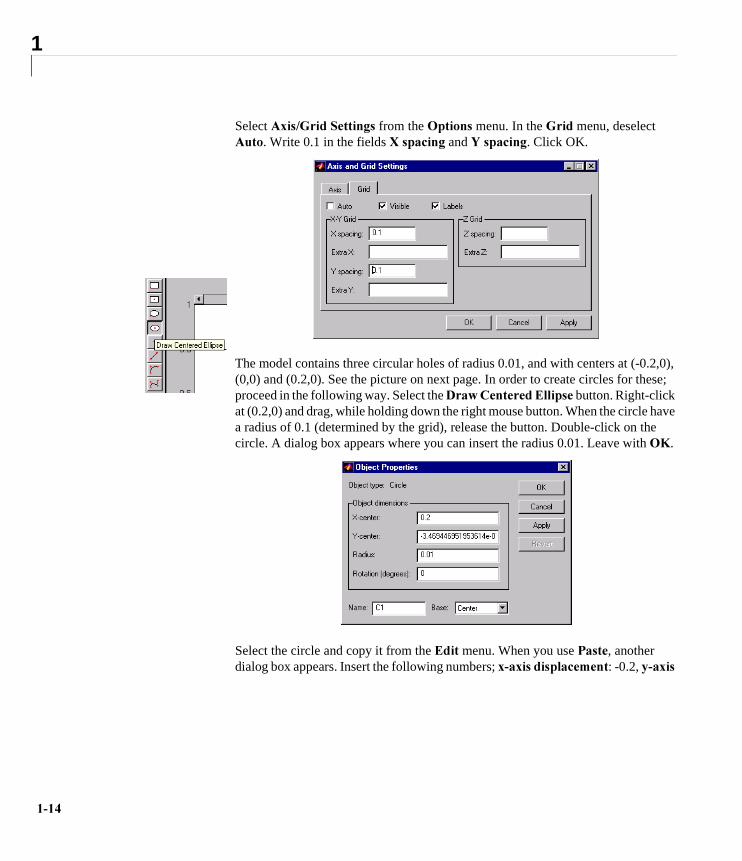
Select $[LV*ULG6HWWLQJV from the 2SWLRQV menu. In the *ULG menu, deselect $XWR. Write 0.1 in the fields ;VSDFLQJ and <VSDFLQJ. Click OK.

The model contains three circular holes of radius 0.01, and with centers at (-0.2,0), (0,0) and (0.2,0). See the picture on next page. In order to create circles for these; proceed in the following way. Select the 'UDZ&HQWHUHG(OOLSVH button. Right-click at (0.2,0) and drag, while holding down the right mouse button. When the circle have a radius of 0.1 (determined by the grid), release the button. Double-click on the circle. A dialog box appears where you can insert the radius 0.01. Leave with 2..

Select the circle and copy it from the (GLW menu. When you use 3DVWH, another dialog box appears. Insert the following numbers; [D[LVGLVSODFHPHQW: -0.2, \D[LV


GLVSODFHPHQW: 0 and QXPEHURIUHSHDWV: 2. Use the zooming possibility provided

by buttons on the main (upper) toolbar to inspect the result closer. The three circles will now appear in the places where the holes in the figure on next page are situated.

Draw a rectangle by pressing the 'UDZ5HFWDQJOH button (top), then clicking with the mouse on (-0.4, -1), dragging to (0.4,1), and finally releasing the button.

Select all objects (ctrl-a) and subtract the circles from the rectangle, using the difference button to the left (move the mouse over the buttons to inspect their functions).

1

You should now have obtained the following geometry.

Enlarged part of the geometry

The small circles are three anodes at zero potential, while the upper and lower sides of the rectangle are electrodes held at a potential of 100V. On the vertical edges symmetry conditions are applied, since the real detector consists of an array of many electrodes. The space charge due to secondary electrons is totally insignificant. With this information we can specify the boundary conditions and the material properties in the PDE specification.

Press the %RXQGDU\&RQGLWLRQ button δΩ on the upper toolbar. The boundaries are visible as arrows. Their default value is zero voltage, i.e. a Dirichlet condition, which is marked by solid arrows. Neumann- or Generalized Neumann conditions are shown as dashed arrows.

Open the 6SHFLI\%RXQGDU\&RQGLWLRQV dialog box from the %RXQGDU\ menu. Select among the numbers in the left table. When you select a number, the corresponding boundary becomes colored. You can select several boundaries simultaneously. You can also select boundaries in the dialog box, by selecting edges in the main GUI.


The three cathodes are already grounded by default. However, the upper and lower electrodes must be set to 100 V. The vertical edges should be set to LQVXODWLRQV\PPHWU\. Notice that the boundary lines become dashed when this boundary condition is selected. This indicates that they are Neumann conditions.

Press 2..

Next, open the 3'(6SHFLILFDWLRQ dialog box in the 3'( menu. Select domain 1 in the left table. We have vacuum and the electrons can be disregarded. Thus the space charge density is zero and the dielectric constant of no interest. Change 6SDFHFKDUJHGHQVLW\ to zero.

Press the 0HVK0RGHbutton to enter the mesh mode. A mesh is automatically generated. This initial mesh is the same as the one generated by the triangle button on the upper toolbar. If we would have wanted to refine the mesh, this could have

1

been done by pressing the 5HILQH0HVK button. In our case, however, an adaptive mesh solver will be used to refine the mesh selectively during the solution.

Change the solver parameters by pressing the 6ROYHU3DUDPHWHUV button. Alternatively, this can be done by selecting 3DUDPHWHUV in the 6ROYHU menu. Check


the $GDSWLRQ box in the general page, and then solve the problem (the equality sign button).

1

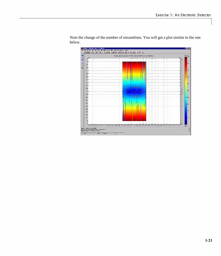
In order to see the field lines in the plot, press the 3ORW3DUDPHWHUV button (a question mark on top of a Matlab symbol). Check the )ORZSORW check box on the )ORZ page. Then select electric field in the following way.


Note the change of the number of streamlines. You will get a plot similar to the one below.


Exercise 2: Mechanical Component ModelFor this example you need the file comp.dxf, which can be downloaded together with the rest of the course material.

In this exercise a plane stress model is created in the Structural Mechanics Engineering Module (SME). You can read more about this module in the introduction. We are going to look at different possibilities to analyse the properties of the model. These include static analysis, as well as eigen frequency and frequency response analysis.

Static Analysis• Choose 3ODQH6WUHVV/LQHDU6WDWLFin 6WUXFWXUDO0HFKDQLFV0RGXOH in the 0RGHO1DYLJDWRU (select 1HZfromthe)LOH menu).

Options and Settings

You do not need any settings in this problem.

1

Draw Mode

• Import the DXF file comp.dxf using ,QVHUWIURP)LOH';)ILOH on the )LOHmenu.

The DXF file is located in your course directory.

• First you should solidify the circles. Select all curve objects on a circle. This can be done, either by using the ctrl-key while clicking on each of the curve elements with the mouse, or by holding down the left mouse button and dragging it over the circle. Be sure that you only select curve objects of the circle. Coerce the selected object to a solid by pressing the &RHUFHWR6ROLG button on the 'UDZ toolbar (left, third from the bottom). Do this for both circles.

• Select all outer edge curve objects and coerce to a solid.

• You should now have three objects. Select them all (ctrl-a).

• Remove the circles by pressing the 'LIIHUHQFH button on the 'UDZ toolbar.

Elements Mode

The imported component is drawn using meter as length scale so we use SI units for the material data.

• Specify elements according to the following table, using 6SHFLI\(OHPHQWV from the (OHPHQWVmenu.:

• Enter material data according to the following table, using 6SHFLI\0DWHULDO from the (OHPHQWVmenu.:

Subdomain 1

Element Plane stress, 3-node triangle

Subdomain 1

E 2.1e11

nu 0.3

t 4e-3

rho 7.85e3


Load Mode

Open the 6SHFLI\/RDGVDQG&RQVWUDLQWVdialog box under the /RDGmenu. Edge 12 should have the load 15e6 in the x-direction. Notice the arrows that denote the load. Constrain edge 1 in the x- and y- directions, by checking 5[ and 5\ for edge 1. Leave the dialog box, using OK.

Mesh Mode

• Select 3DUDPHWHUV from the 0HVK menu.

• Enter 3e-3 as 0D[HGJHVL]HJHQHUDO in the 0HVK3DUDPHWHUV dialog box.

• Select ,QLWLDOL]HPHVK, using e.g. the triangle button in the upper toolbar.

Solve Mode

• Solve the problem by pressing the equal sign button.

Plot Mode

Plot the von Mises stresses and the deformed shape.

• Check 'HIRUPHGVKDSHand 6XUIDFH in the *HQHUDO page in the 3ORW3DUDPHWHUV dialog box.

Edge all

t 4e-3

1

• Select von Mises stress (vonmises)as 6XUIDFHH[SUHVVLRQ, in the 6XUIDFH page.

Eigenfrequency AnalysisLet us now study the eigenfrequencies of the component.

• Select 6ROYHU3DUDPHWHUV from the 6ROYHmenu and choose (LJHQIUHTXHQF\ as $QDO\VLVon the general page.

• Solve the problem once more.

Go to the 3ORW3DUDPHWHUV dialog box and select the second eigenfrequency, at 1.4 kHz.


Frequency ResponseIn a frequency response analysis, the steady state response from harmonic loading of the model, is studied. The loads can be described as

where the amplitude and phase can be functions of the excitation frequency I.

In the SME module, modal decomposition is used, and the user can specify the eigenfrequency to be used in the frequency response analysis. The damping can be specified individually.

The excitation frequency can be specified in a number of ways. In this example we will use the default settings, which means that we excite with frequencies spread around the eigenfrequencies.

• Open 6ROYHU3DUDPHWHUV.

) W( ) $ I( ) 2πI γ I( )+( )sin=

1

• Select )UHTXHQF\5HVSRQVH as $QDO\VLVon the *HQHUDOpage.

• Solve once more

Let us plot the result from an excitation with a frequency equal to the second eigenfrequency.

• Go to 3ORW3DUDPHWHUV and select the frequency 1.4 kHz.

Finally, we would like to view the deformation as a function of frequency in a x-y plot.

• First select /DEHOV, 6KRZ3RLQW/DEHOV in the 2SWLRQV menu. We will study the x-deformation where the load is applied (point 27).

• Go to 3ORW3DUDPHWHUV and select the 1RGH page. Insert 27 as the 1RGHQXPEHUWRSORW and press the 1RGH3ORW button. The amplitude of the response is shown in the figure below.

As expected, there is a peak in the displacement around the eigenfrequency, but the response is damped for higher frequencies.

1


Diffusion in Isothermal Laminar Flow Along a Flat Plate

IntroductionIn the transport of chemical species in laminar flow, the flux time scale for diffusion compared to convection differs, in most cases, by several orders of magnitude. This can instructively be visualized by modeling these transports mechanisms in the simplest possible geometry. This is neatly shown in [1], where the diffusion in laminar flow along a soluble flat plate is treated analytically. However, the analytical solution requires a fairly large degree of simplification, where even this does not provide a straight-forward solution.

In this example, we will treat the same type of problem with a minimum of simplification. This simple model serves as an introduction to the modeling of systems where a mass balances is coupled to a momentum balance, and where the flux of dissolved species in a fluid is given by diffusion and convection.

We will study the concentration and flow distributions along a flat plate in a parallel channel. We will assume that a constant flux of a dissolved species, perpendicular to the surface, is generated along the flat plate. The solution will generate the developing structures of the viscous and diffusion layers in the parallel channel.

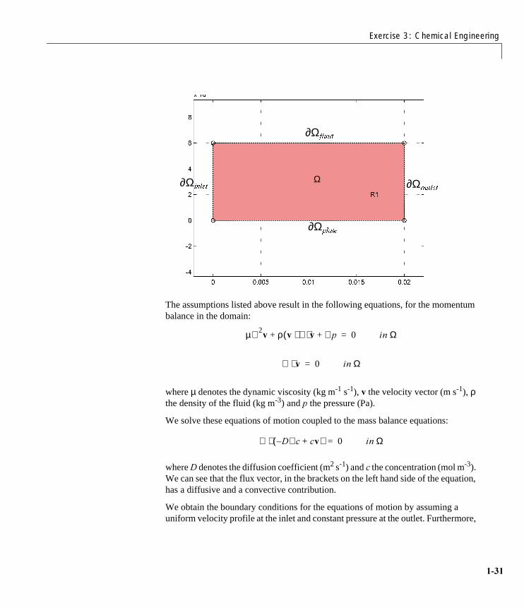
Definition of the problemWe treat the problem with one diffusing species, dissolved in water at room temperature. The geometry of the domain in this model is the simplest possible; a rectangle of 6 times 20 mm, see the below figure. The fluid inlet to our system is situated at the left boundary and the outlet at the right. The plate is represented by the lower boundary and symmetry is assumed at the top. The diffusing species is produced at the surface of the plate.

We use the Navier-Stokes equations, in combination with the continuity equation and a mass balance equation, for one dissolved chemical species. The transport of this species takes place by diffusion and convection. We further assume that the production of the diffusing species, at the surface of the plate, does not influence the viscosity and density of the fluid.


The assumptions listed above result in the following equations, for the momentum balance in the domain:

where µ denotes the dynamic viscosity (kg m-1 s-1), Y the velocity vector (m s-1), ρ the density of the fluid (kg m-3) and S the pressure (Pa).

We solve these equations of motion coupled to the mass balance equations:

where ' denotes the diffusion coefficient (m2 s-1) and F the concentration (mol m-3). We can see that the flux vector, in the brackets on the left hand side of the equation, has a diffusive and a convective contribution.

We obtain the boundary conditions for the equations of motion by assuming a uniform velocity profile at the inlet and constant pressure at the outlet. Furthermore,

Ω

∂ΩSODWH

∂ΩIOXLG

∂ΩRXWOHW∂ΩLQOHW

µ∇2Y ρ Y ∇⋅( )Y ∇S+ + 0= LQ Ω

∇ Y⋅ 0= LQ Ω

∇ ' F FY+∇–( )⋅ 0= LQ Ω

1

we assume symmetry along the boundary towards the free fluid. These assumptions give the following boundary conditions for the equations of motion:

We additionally obtain the corresponding boundary conditions, for the mass balance equations, by assuming that the concentration is known at the inlet and at the symmetry boundaries. We also know the production rate of the diffusing species at the surface of the plate, and assume that the dominating transport process in the direction of the flow, at the outlet, is transport by convection. This can be formulated by the following equations:

The condition that determines the concentration at the symmetry boundary is only valid in the case when the diffusion layer does not reach this boundary. This assumption will be validated or falsified in the solution.

Y Q⋅ Y0= DW ∂ΩLQOHW

Y Q⋅ 0= DW ∂ΩI OXLG

Y 0 0,( )= DW ∂ΩSODWH

S 0= DW ∂ΩRXWOHW

F F0= DW ∂ΩLQOHW

F F0= DW ∂ΩIOXLG

' F FY+∇–( ) Q⋅ N= DW ∂ΩSODWH

' F FY+∇–( ) Q⋅ FY( ) Q⋅= DW ∂ΩRXWOHW


Solving the problem using the Graphical User InterfaceSelect ,QFRPSUHVVLEOH1DYLHU6WRNHV, from the 0XOWLSK\VLFV menu in the 0RGHO1DYLJDWRU, and add it as an application mode by moving it to the right field with the arrow button. Press 2..

Options and Settings

• Open $[LV*ULG6HWWLQJV in the 2SWLRQV menu. Unselect $[HV(TXDO and set the axis settings according to the table below: Then, go to the *ULGdialog box and set the grid values according to the table. You have to uncheck the $XWRcheckbox. Press 2..

• Enter the following variable names, for later use, in the $GG(GLW9DULDEOHV window, in the 2SWLRQV menu. Then press 2.

Axis Grid

X min -0.001 X spacing 0.005

X max 0.021

Y min -0.002 Y spacing 0.002

Y max 0.008

Name Expression

rho 1e3

miu 1e-3

D1 5e-9

flux 5.2e-2

vo 0.01

c1o 0

1

Draw Mode

• Press the 'UDZ5HFWDQJOH button in the 'UDZtoolbar. Press the left mouse button at the position (0,0) and draw to (0.02,0.006). Then release the mouse button.You have made a rectangle with the name R1.

Boundary Mode

• Select 6SHFLI\%RXQGDU\&RQGLWLRQV from the %RXQGDU\ menu. Enter boundary coefficients according to the following table. Then press 2.

Boundary 1 2 3 4

Type Inflow No-slip Slip Outflow

u vo

v 0

p 0


PDE Mode

We can start by defining the coefficients for the Navier-Stokes equations, which are the density and viscosity of the fluid, in this case water.

• Select 3'(6SHFLILFDWLRQVfrom the 3'( menu. Enter the PDE coefficients, in subdomain 1, according to the following table. Then press 2.

We are now ready to define the mass transport equations for the diffusing species that is being produced at the surface of the plate. We do this by adding a new model equation in the 0XOWLSK\VLFV0RGH.

Multiphysics Mode

• Select $GG(GLW0RGHVin the 0XOWLSK\VLFV menu. Choose3'(JHQHUDOIRUP, label your application mode with the name, massbal, and your Dependent variable, c1. This is done in the two bottom fields, before moving the selected mode to the right.

Subdomain 1

ρ rho

η miu

1

• Add the new application by moving it to the right field with the arrow button. Press 2.. You should now be in the YDULDEOHJHQHUDOIRUP3'(PDVVEDOPRGH, as you can see at the top of the main GUI window. Check this by selecting the 0XOWLSK\VLFV menu.

Boundary Mode

• Enter boundary coefficients according to the following table. Press 2..

PDE Mode

We define the flux vector, in the 3'(0RGH, as an expression that consists of a diffusion and a convection term.

• Enter the PDE coefficients according to the following table. Note that Γ is a vector. Thus, there is a space in the middle of the expression. Press 2..

Mesh Mode

This example requires a fairly dense mesh since the Reynolds number is relatively high. For that purpose, we define a maximum element size for the edge that represents the flat plate. This requires that we identify the edge number of our geometry. Select 2SWLRQ, /DEHOV6KRZ(GJH/DEHOV in Draw Mode. In 0HVK0RGH:

• Choose 3DUDPHWHUV and press the button labeled 0RUH.

Boundary 1,3 2 4

G 0 flux -c1.*u

R -c1+c1o 0 0

Subdomain 1

Γ -D1.*c1x+c1.*u -D1.*c1y+c1.*v

F 0

da 0


• In the field 0D[HOHPHQWVL]HIRUHGJHV, set the maximum element size for edge 2 to 1e-4. This done by inserting “2 1e-4” in the field.

• Press 5HPHVK and then 2..

• Refine the mesh once, using the 5HILQH0HVK, button on the main toolbar, or by selecting 5HILQH0HVK in the 0HVK menu.

Solve Mode

• Select 6ROYHU3DUDPHWHUV on the main toolbar or in the 6ROYH menu. Check that the 6WDWLRQDU\QRQOLQHDUVROYHU is used. 6WUHDPOLQHGLIIXVLRQ should be off.

1

• Set the 7ROHUDQFH to 1e-8. This is done by selecting the dialog box 1RQOLQHDU, and inserting 1e-8 instead of 1e-4 in the bottom field. Solve the problem by pressing the 6ROYH button. The solution takes a couple of minutes.

Plot Mode

The default plot shows the concentration of the reacting species in the solution (in mole m-3). The most interesting result from this simulation is a comparison between the thickness of the viscous layer and of the diffusion boundary layer, which is often given in the Schmidt number (Sc). We can obtain a notion of this relation by plotting the results in a 3-D surface plot. To do this, choose to plot the velocity field as


6XUIDFHH[SUHVVLRQ, and the concentration as +HLJKWH[SUHVVLRQ in the 3ORW3DUDPHWHUVdialog window. After rotating we obtain the resulting plot:

The difference between the viscous and diffusion layers can be clearly seen, in the figure above, by the amount that they extend into the fluid. This difference can be seen even more clearly if we reverse the plotting instructions. In order to do this, plot

1

the concentration as 6XUIDFHH[SUHVVLRQ and the velocity field as +HLJKWH[SUHVVLRQ in the 3ORW3DUDPHWHUV dialog window. Rotate freely to generate a suitable view.

In addition, we can see in the above figure that we have almost a fully developed laminar flow, at the outlet of the domain, which supports our assumption of a constant pressure along this boundary.

References [1] R. Bird, W. Stewart and E. Lightfoot, ³7UDQVSRUW3KHQRPHQD´, John Wiley & Sons, New York, 1960.

minicourse on femlab

Documents