femlab introductory
TRANSCRIPT

How to contact COMSOL:
BeneluxCOMSOL BVRöntgenlaan 192719 DX ZoetermeerThe [email protected]
DenmarkCOMSOL A/SRosenkæret 11CDK-2860 SøborgPhone: +45 39 66 56 50Fax: +45 39 66 56 [email protected]
FinlandCOMSOL OYLauttasaarentie 52FIN-00200 HelsinkiPhone: +358 9 2510 400Fax: +358 9 2510 [email protected]
FranceCOMSOL France19 rue des bergersF-38000 GrenoblePhone: +33 (0)4 76 46 49 01Fax: +33 (0)4 76 46 07 [email protected]
GermanyFEMLAB GmbHBerliner Str. 4D-37073 GöttingenPhone: +49-551-99721-0Fax: [email protected]
NorwayCOMSOL ASVerftsgata 4NO-7485 TrondheimPhone: +47 73 84 24 00Fax: +47 73 84 24 [email protected]
SwedenCOMSOL ABTegnérgatan 23SE-111 40 StockholmPhone: +46 8 412 95 00Fax: +46 8 412 95 [email protected]
SwitzerlandCOMSOL ABRepräsentationsbüro SchweizTechnoparkstrasse 1CH-8005 ZürichPhone: +41 (0)44 445 2140Fax: +41 (0)44 445 [email protected]
United KingdomCOMSOL Ltd.Studio G8 Shepherds Building Rockley RoadLondon W14 0DAPhone:+44-(0)-20 7348 9000Fax: +44-(0)-20 7348 [email protected]
United States COMSOL, Inc.1 New England Executive ParkSuite 350Burlington, MA 01803Phone: +1-781-273-3322Fax: [email protected]
COMSOL, Inc.1100 Glendon Avenue17th FloorLos Angeles, CA 90024Phone: +1-310-689-7250Fax: [email protected]
COMSOL, Inc.744 Cowper StreetPalo Alto, CA 94301Phone: +1-650-324-9935Email: [email protected]
For more representatives, see www.comsol.com/contactCompany home pagewww.comsol.comProduct [email protected]
FEMLAB user forumswww.comsol.com/support/forums
FEMLAB MEMS Modeling Course COPYRIGHT 1994–2005 by COMSOL AB. All rights reserved
Patent pending
The software described in this document is furnished under a license agreement. The software may be used or copied only under the terms of the license agreement. No part of this manual may be photocopied or reproduced in any form without prior written consent from COMSOL AB.
FEMLAB is a registered trademark of COMSOL AB.
Other product or brand names are trademarks or registered trademarks of their respective holders.
Version: 3.1, May 2005 FEMLAB 3.1i


i | C O N T E N T S
C O N T E N T S
Preface 2
Tube in Current 3
Introduction to the Lesson . . . . . . . . . . . . . . . . . . . 3
Key Instructive Elements . . . . . . . . . . . . . . . . . . . . 3
Currents in Aluminum Deposit 20
Model Description . . . . . . . . . . . . . . . . . . . . . . 21
Current Balance and Heat Balances in a Two-dimensional cross section . . 22
Using the Graphical User Interface . . . . . . . . . . . . . . . . 23
Convergence analysis (optional) . . . . . . . . . . . . . . . . . 37
The Three-Dimensional Current and Heat Balances . . . . . . . . . 39
Creating the 3D Model Geometry . . . . . . . . . . . . . . . . 40
Summary of Equations . . . . . . . . . . . . . . . . . . . . . 47

C O N T E N T S | ii

| 1
1
F E M L A B I n t r o d u c t o r y C o u r s e

2 | C H A P T E R 1 : F E M L A B I N T R O D U C T O R Y C O U R S E
P r e f a c e
Mathematical modeling has become a very important part of the research and development work in engineering and science. Competitive edge requires speed on the path between idea and prototype, and mathematical modeling and simulation provides a valuable shortcut for understanding both qualitative and quantitative aspects of scientific and engineering design. To your assistance, FEMLAB 3 offers state-of-the art performance, being built from the foundation with Java3D interface and C/C++ solvers.
This course gives you an introduction to modeling in FEMLAB 3 and takes you through all the steps of the modeling process, from drawing or geometry import, to parametric analysis.
The exercises do not require any prior expertise in mathematical modeling or FEMLAB use to be rewarding.
Enjoy your modeling!
3 | C H A P T E R 1 : F E M L A B I N T R O D U C T O R Y C O U R S E
T ub e i n C u r r en t
Introduction to the Lesson
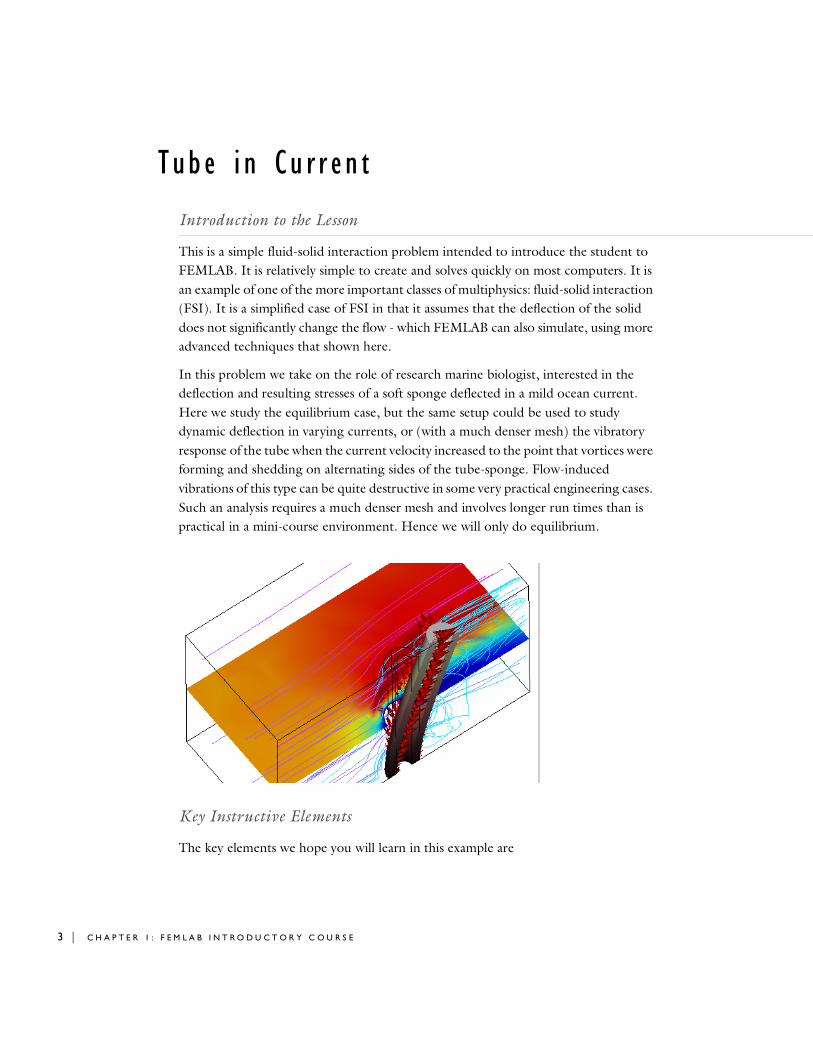
This is a simple fluid-solid interaction problem intended to introduce the student to FEMLAB. It is relatively simple to create and solves quickly on most computers. It is an example of one of the more important classes of multiphysics: fluid-solid interaction (FSI). It is a simplified case of FSI in that it assumes that the deflection of the solid does not significantly change the flow - which FEMLAB can also simulate, using more advanced techniques that shown here.
In this problem we take on the role of research marine biologist, interested in the deflection and resulting stresses of a soft sponge deflected in a mild ocean current. Here we study the equilibrium case, but the same setup could be used to study dynamic deflection in varying currents, or (with a much denser mesh) the vibratory response of the tube when the current velocity increased to the point that vortices were forming and shedding on alternating sides of the tube-sponge. Flow-induced vibrations of this type can be quite destructive in some very practical engineering cases. Such an analysis requires a much denser mesh and involves longer run times than is practical in a mini-course environment. Hence we will only do equilibrium.
Key Instructive Elements
The key elements we hope you will learn in this example are

TU B E I N C U R R E N T | 4
1 How to create and manipulate simple 3D geometries in FEMLAB
2 Find geometric symmetry planes to reduce the model size.
3 Practice simulating flow and structural analyses
4 How to define materials, set boundary conditions, and link sets of physics together
5 Use of the parametric solver to plot both system and user-created functions vs. parameter
6 Demonstrating a variety of FEMLAB’s postprocessing capabilities including animations
P H Y S I C S
In this problem seawater is flowing over and around a single branch tubular sponge - which is deflected by this flow. The two key physics involved are incompressible fluid flow (for the seawater) and 3-D static structural analysis. We might also represent the tube with structural shells, but in this case the wall thickness of the tube is relatively thick compared to the diameter. The flow over the tube creates forces on the surface due to pressure and shear stress. These forces load the tube structurally and deflects it. The sponge walls are quite elastic and bend relatively easily in these mild currents. The problem is assumed to be symmetric down the center plane - eliminating the possibility of simulating side-to-side vibrations. Finally, the velocity profile of the ocean current this close to the bottom has been found to typically follow a variety of relations, depending on the up-current profile of the bottom. We will simulate the problem with one such profile.
P R O B L E M S E T U P
1 Start FEMLAB by double clicking on the FEMLAB icon on your screen. The FEMLAB Model Navigator will launch.
2 Select 3D as the Space Dimension
3 Then in the list of Physical Models select FEMLAB > Fluid Dynamics > Incompressible
Navier Stokes. To be sure you have the right application mode, the Application mode
5 | C H A P T E R 1 : F E M L A B I N T R O D U C T O R Y C O U R S E
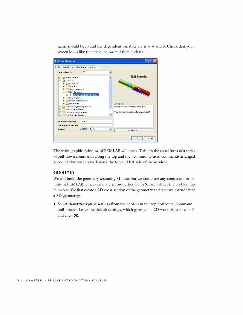
name should be ns and the dependent variables are u v w and p. Check that your screen looks like the image below and then click OK.
The main graphics window of FEMLAB will open. This has the usual form of a series of pull-down commands along the top and then commonly-used commands arranged as toolbar buttons arrayed along the top and left side of the window.
G E O M E T R Y
We will build the geometry assuming SI units but we could use any consistent set of units in FEMLAB. Since our material properties are in SI, we will set the problem up in meters. We first create a 2D cross-section of the geometry and later we extrude it to a 3D geometry:
1 Select Draw>Workplane settings from the choices in the top horizontal command pull-downs. Leave the default settings, which gives you a 2D work plane at z = 0 and click OK.

TU B E I N C U R R E N T | 6
62 Select Draw > Specify Objects > Circle and enter 0.001 in the Radius field. Leave the other fields at their default values and click OK to create the circle.
3 Select the Zoom Extents button (the one with the Red Cross) in the top horizontal toolbar.
We will create the hollow center by creating another circle and then subtracting it from the first one.
4 Select Draw > Specify Objects > Circle and enter 5e-4 in the Radius field. Leave the other fields at their default values and select OK to create the circle.
5 To subtract the inside from the outside choose Edit > Select All and then the Difference button on the left vertical toolbar (just above the +-/x button).
Since the problem is symmetric, we can cut the tube (so far the circle before extruding it to 3D) in half.
6 Select Draw > Specify Objects > Rectangle and enter Width = 0.016 and Height = 0.008. Leave the Base Position to be the Corner and enter x = -0.008. Click OK.

7 | C H A P T E R 1 : F E M L A B I N T R O D U C T O R Y C O U R S E
7 Select the Zoom Extents button (the one with the Red Cross) in the top horizontal toolbar.
8 With the rectangle still highlighted, select Edit > Copy (or select Ctrl-c). Then, select Edit > Select all and click the Intersection tool button on the left vertical toolbar.
You should see half of the hollow circle cut vertically on the symmetry plane.
9 Paste the rectangle back in by selecting Edit > Paste and leave the Displacements to zero. Last of all we remove the inner semi-circle from the rectangle.
10 Select Draw > Specify Objects > Circle and enter 0.001 in the Radius edit field. Leave the other fields at their default values and click OK to create the circle.
11 Select Draw > Create Composite Object and enter R1-C1 in the Set Formula edit field. Click OK.

TU B E I N C U R R E N T | 8
12 Select Draw > Extrude and select both CO2 and CO3. Enter 0.01 in the Distance edit field and click OK.
13 To see the geometry in a shaded mode, select the Headlight button on the left vertical toolbar.
Your geometry should look like what is shown below. If you had trouble, you can load a completed geometry at this point. To do so, select File > New and load the file: Tube_in_Current_GEOM.fl Only do this if your geometry does not look like that below.

9 | C H A P T E R 1 : F E M L A B I N T R O D U C T O R Y C O U R S E
We have defined the geometry and created introduced the flow physics to the problem. We next need to define the material properties and boundary conditions for the flow problem and then introduce and do the same for the structural part of the problem.
M A T E R I A L P R O P E R T I E S - F L OW
We first assign material properties for the flow, under the Physics pull-down commands
TU B E I N C U R R E N T | 10
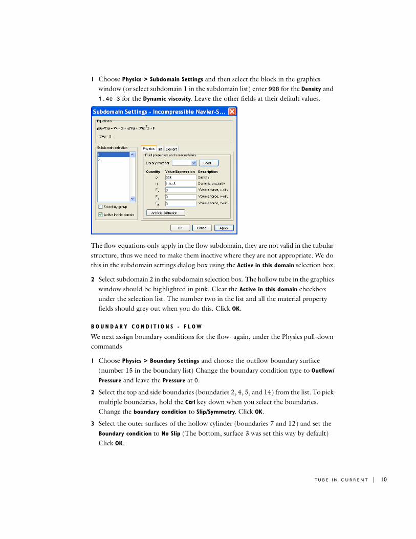
1 Choose Physics > Subdomain Settings and then select the block in the graphics window (or select subdomain 1 in the subdomain list) enter 998 for the Density and 1.4e-3 for the Dynamic viscosity. Leave the other fields at their default values.
The flow equations only apply in the flow subdomain, they are not valid in the tubular structure, thus we need to make them inactive where they are not appropriate. We do this in the subdomain settings dialog box using the Active in this domain selection box.
2 Select subdomain 2 in the subdomain selection box. The hollow tube in the graphics window should be highlighted in pink. Clear the Active in this domain checkbox under the selection list. The number two in the list and all the material property fields should grey out when you do this. Click OK.
B O U N D A R Y C O N D I T I O N S - F L O W
We next assign boundary conditions for the flow- again, under the Physics pull-down commands
1 Choose Physics > Boundary Settings and choose the outflow boundary surface (number 15 in the boundary list) Change the boundary condition type to Outflow/
Pressure and leave the Pressure at 0.
2 Select the top and side boundaries (boundaries 2, 4, 5, and 14) from the list. To pick multiple boundaries, hold the Ctrl key down when you select the boundaries. Change the boundary condition to Slip/Symmetry. Click OK.
3 Select the outer surfaces of the hollow cylinder (boundaries 7 and 12) and set the Boundary condition to No Slip (The bottom, surface 3 was set this way by default) Click OK.

11 | C H A P T E R 1 : F E M L A B I N T R O D U C T O R Y C O U R S E
4 Finally, choose the inflow boundary (boundary 1). Here we specify the inflow velocity. Change the boundary condition type to Inflow/outflow velocity.
Normally we would just enter numerical values for the velocity. In FEMLAB, anywhere you can enter a number you can also enter an equation. For this problem the velocity follows a known profile that is a function of the vertical depth - thus a function of z in our coordinate system. In this case, we will let the velocity vary with the fifth-root of the depth as Vin(z/0.01)(1/5). Additionally, we would like to change this velocity parametrically. Thus we will write the profile as a function of z and of a (yet to be defined) constant V_in. V_in will be the magnitude of the velocity at the top of our domain, which we will eventually vary from 1 to 5 cm per second.
5 To finish specifying the inlet velocity boundary: Enter V_in*(z/.01)^0.2 in the u0 field and leave the other two components as zero. Click OK and close the window.
6 To define the constant: Select Options > Constants and enter V_in as the Name and 0.03 as the Expression. Click OK. Be sure you get the right number of decimal places here! Similarly, you might want to double check the boundary expression in the previous step. If you inadvertently enter too large a velocity, the character of the flow may change from steady to unsteady and there simply is not a stationary solution for the solver to find. It, of course, does not know this and continues iterating until it reaches its maximum iteration limit and gives up.
At this point we could either introduce the structural equations and their corresponding material properties and boundary conditions or we could check if the flow part is set up as planned. In multiphysics problems it is always wise to check them on each major step. This makes debugging the problem later easier if you made mistakes along the way. Lets be prudent and check what we have thus far.

TU B E I N C U R R E N T | 12
M E S H A N D S O L V E F O R F L O W
FEMLAB has a very sophisticated mesh algorithm which meshes the problem based on the geometry you have defined. Because this is a class problem and not a true research problem we would like the problem to be as small as possible, so that each solution will converge quickly and so that we do not inadvertently define a problem that is too large for classroom computers.
Thus we will first change the default mesh parameters that FEMLAB uses to mesh the problem.
1 Select Mesh > Mesh Parameters and change the Predefined mesh sizes pull-down field at the top of the window to Extra Coarse. Click Remesh and OK. You should get around 2500 elements.
FEMLAB also sets up the solver parameters based on the problem you have defined. This is a 3D flow problem, which in general, could be quite large. Thus FEMLAB selects the solver expecting large system matrices and large memory demands. For this particular geometry, the problem is quite small and we can save ourselves quite a bit of time if we select a direct solver instead of the predefined iterative one.
1 Select Solve > Solver Parameters and change the Linear System Solver (in the upper left side of the menu) to Direct (UMFPACK). Leave everything else at its default. Click OK.
2 Select Solve > Solve Problem. After a short time you should see the figure on the right: (You can toggle off the headlight to remove shading and thus brighten the image)
13 | C H A P T E R 1 : F E M L A B I N T R O D U C T O R Y C O U R S E
1 Select Postprocessing > Plot Parameters and pick the Slice tab at the top. In the Slice subwindow change the x-levels to 3, the y-levels to 0, and the z-levels to 1. Click Apply.
2 While still in the postprocessing window, select the Arrow tab at the top. In the Arrow subwindow, set the x-points to 15, the y-points to 10 and the z-points to 7. Change to Arrow type to 3D arrow. Clear the Auto scale factor checkbox and enter the Scale factor to be 1.3. Finally, select the Arrow plot checkbox in the upper left corner of the window. (Don’t click Apply yet!)
Before you add the 3D arrows to the result plot, you may want to save your model. Sometimes the graphics cards on seminar computers do not have much memory in them. Arrow plots, particularly 3D arrow plots, call for extra memory on this card. If the graphics card has a small memory, the computer sometimes can crash and your model (if not previously saved) will be gone! If this is a new computer to you - I suggest you save your model now (File > Save).
3 Select Apply to add the arrows to your plot.
4 Select the Streamline tab and change the Number of streamlines to 40. Select the Streamline checkbox in the upper left corner. In the Streamline color box, select the Use expression to color streamlines radio button and then select the Color Expression button. Leave the Expression as U_ns but change the Colormap to cool. Clear the Colorscale checkbox and click OK to close the color expression window. Then click OK to close the Plot parameters window.
5 To turn off the coordinate system grid on the screen, select the Options > Axis/Grid
Settings and clear the Visible checkbox in the Axis window. Click OK.
You should see the plot below. You can toggle between orientations by selecting the XY-View button and the Default View button (both located on the left vertical toolbar).

TU B E I N C U R R E N T | 14
We would like to see the fluid-loading on the post. FEMLAB calculates this for us for all surfaces in the model. Graphically we only want to see the post loading. To set this up we can define a variable for the surface loading that only is defined on the post.
1 Pick Options > Expressions > Boundary Expressions and select the outer surface of the post (boundaries 7 and 12). Enter P_Post as the Name and T_x_ns for the Expression. Click OK.
2 Select Solve > Update Model to evaluate this variable without recalculating the solution.
3 Select Postprocessing > Plot Parameters and pick the Boundary tab. Enter -P_Post in the Expression field (remember the negative!) and select the Boundary checkbox. Click the General tab and clear both the Arrow plot and Slice plot types. Click OK. Reorient the view to see the x-component of the drag per unit area on the post.
S E T U P S T R U C T U R A L P R O B L E M
1 Select Multiphysics > Model Navigator. In the list of Physical Models select FEMLAB >
Structural Mechanics > Solid, Stress-Strain > Static Analysis. To be sure you have the right application mode, the Application mode name should be solid3 and the

15 | C H A P T E R 1 : F E M L A B I N T R O D U C T O R Y C O U R S E
Dependent variables are u2 v2, and w2. Select Add (at the top right side), then click OK to close the window.
2 Select Physics > Subdomain Settings and choose subdomain 1 (the flow volume). The structural equations are not applied in this subdomain and thus need to be inactivated. Clear the Active in this domain checkbox to turn them off. Click Apply.
3 Select subdomain 2 (the hollow cylinder) to define it’s material properties. Enter 2e3 for Young’s Modulus, 0.3 for the Poisson’s ratio and 1004 for the Density. Click OK.
4 Select Physics > Boundary Settings and enter the boundary conditions as follows (Notice the negative signs on the forces!) Once done, click OK.
The three surface stresses, T_x_ns, T_y_ns and T_z_ns are application variables that are internally calculated by the Navier Stokes equation mode. They are the total fluid force per unit area on a given surface pushing back on the fluid. Using them as surface
BOUNDARIES LOCATION BOUNDARY CONDITION VARIABLE EXPRESSION
7, 12 Click Load Tab Fx
Fy
Fz
-T_x_ns
-T_y_ns
-T_z_ns
8 Constraints: Select all three: Rx, Ry, Rz Rx
Ry
Rz
0
0
0
6, 13 Constraints: Select only Ry Ry 0

TU B E I N C U R R E N T | 16
force boundary conditions in the structural mechanics equations links the flow to the deformation. Again, remember to set the surface force as the negative of the fluid surface stress!
S O L V E F L O W - I N D U C E D D E F O R M A T I O N P R O B L E M
The coupled problem is now completely set up. In this case the two physics (flow and structures) is only linked one way: The deformation depends on the fluid drag force and thus the flow distribution, but the flow (in our model) does not depend on the deformation. This is an example of one-way coupling between the equations. We could reduce the problem size and solve first for flow and then use that solution to solve a second structural deformation solution.
By default, FEMLAB solves everything simultaneously - as if all physics depend on one another. FEMLAB has a solver manager to enable sequential solution of some of the equations in the system. The solver manager is used to manage overall problem size and allow sequential solutions of loosely coupled physics. Again, we will simply solve everything simultaneously here, as if there was bidirectional coupling.
As an aside, this problem could be set up with bidirectional coupling. If the deformation is large the flow clearly depends on the deformation. We can do this in FEMLAB but it involves an advanced technique of setting up and using a governable mesh in the flow subdomain that moves with the bending of the hollow tube. Such a problem has three sets of “physics” that are solved simultaneously: The flow, the structural deformation, and the deformation of the mesh.
1 Click the Solve button (the one with the equals sign) on the top horizontal toolbar.
2 Select Postprocessing > Plot Parameters and select the Arrow tab. Change the Plot
Arrows on selection list (top right) to Boundaries. Change the Predefined quantities to Global Force (solid3). This is the total face load on the cylindrical structure. Select the Arrow plot checkbox in the upper left corner. Click Apply.
3 Click the Slice tab and change the x-slices from 3 to 0. Select the Slice plot checkbox in the upper left corner. Click Apply
4 Select the Boundary tab and change the Predefined quantities to Total displacement
(solid3) and change the Colormap to Pink. Select the Boundary plot checkbox in the upper left corner. Click Apply
5 Finally, select the Deform tab. Clear the Subdomain checkbox under Domain types to deform. Click the Boundary tab in the Deformation Data area and change the Predefined quantities to Displacement (solid3). Clear the Auto scale checkbox and

17 | C H A P T E R 1 : F E M L A B I N T R O D U C T O R Y C O U R S E
change the scale factor to 1. Finally, select the Deformed shape plot checkbox in the upper left and click OK.
P A R A M E T R I C S O L V E R - E F F E C T O F V A R Y I N G F L OW V E L O C I T Y
1 We first define a new variable which is the integral of the x-component of fluid pressure on the cylinder. Select Options > Integration Coupling Variables > Boundary
Integration and select boundaries 7 and 12 (the outer surface of the cylinder). Enter Drag as the Name and enter -T_x_ns as the Expression. (Remember the negative sign!) Click OK.
2 Next, we set up the solver to automatically sweep through a series of parametric values. Go to Solver > Solver Parameters and select Parametric nonlinear in the Solver
TU B E I N C U R R E N T | 18
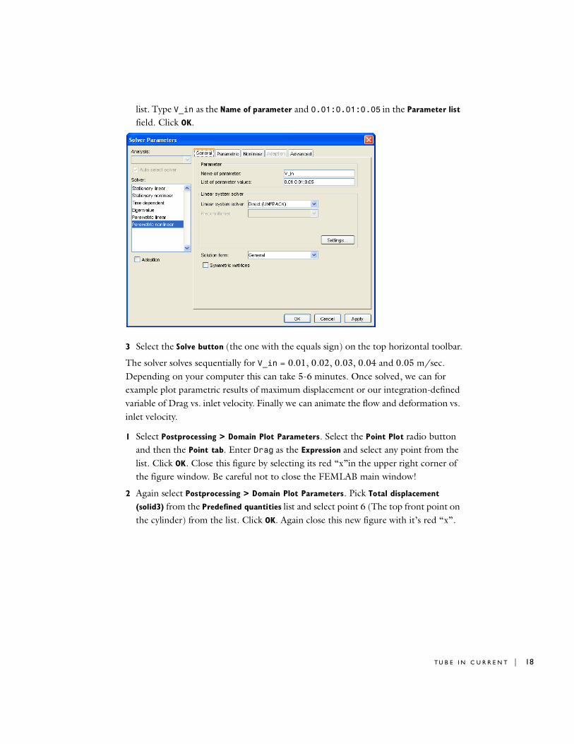
list. Type V_in as the Name of parameter and 0.01:0.01:0.05 in the Parameter list field. Click OK.
3 Select the Solve button (the one with the equals sign) on the top horizontal toolbar.
The solver solves sequentially for V_in = 0.01, 0.02, 0.03, 0.04 and 0.05 m/sec. Depending on your computer this can take 5-6 minutes. Once solved, we can for example plot parametric results of maximum displacement or our integration-defined variable of Drag vs. inlet velocity. Finally we can animate the flow and deformation vs. inlet velocity.
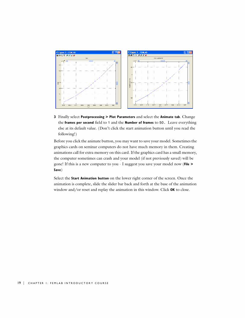
1 Select Postprocessing > Domain Plot Parameters. Select the Point Plot radio button and then the Point tab. Enter Drag as the Expression and select any point from the list. Click OK. Close this figure by selecting its red “x”in the upper right corner of the figure window. Be careful not to close the FEMLAB main window!
2 Again select Postprocessing > Domain Plot Parameters. Pick Total displacement
(solid3) from the Predefined quantities list and select point 6 (The top front point on the cylinder) from the list. Click OK. Again close this new figure with it’s red “x”.
19 | C H A P T E R 1 : F E M L A B I N T R O D U C T O R Y C O U R S E
3 Finally select Postprocessing > Plot Parameters and select the Animate tab. Change the frames per second field to 1 and the Number of frames to 50. Leave everything else at its default value. (Don’t click the start animation button until you read the following!)
Before you click the animate button, you may want to save your model. Sometimes the graphics cards on seminar computers do not have much memory in them. Creating animations call for extra memory on this card. If the graphics card has a small memory, the computer sometimes can crash and your model (if not previously saved) will be gone! If this is a new computer to you - I suggest you save your model now (File >
Save)
Select the Start Animation button on the lower right corner of the screen. Once the animation is complete, slide the slider bar back and forth at the base of the animation window and/or reset and replay the animation in this window. Click OK to close.

C U R R E N T S I N A L U M I N U M D E P O S I T | 20
Cu r r e n t s i n A l um i num Depo s i t
This model treats current conduction and heat generation in an aluminum film deposited on a silicon substrate. The purpose of the model is to investigate the temperature in the device after the current is applied. The model was submitted by M.S. Cohen at Aegis Semiconductors.
The model exemplifies several steps that can be important in the modeling process. It also gives a quick review of the features available for advanced modeling in FEMLAB’s graphical user interface. We will address the following important FEMLAB features:
• The use of predefined physics.
• The definition of a multiphysics problem.
• The expression feature to define physical properties that depend on the solution itself.
• The extraction of design numbers using the postprocessing tools.
• The parametric solver feature that provides fast and efficient parameter screening as well as smooth convergence for highly nonlinear problems.
In addition to the FEMLAB features, several modeling methods are exemplified in the exercise, among them:
• Reduction of the dimension of parts of the problem from three to two dimensions.
• Scaling of the mesh due to large differences in the dimensions of the geometry.
• Control of the obtained results to estimate the validity of the solution.
Apart from theses highlights, we will go through the typical modeling steps, which include:
1 Definition of the geometry.
2 Definition of the physics in the volume and at the boundaries.
3 Meshing.
4 Solving.
5 Postprocessing.
6 Parametric studies.
21 | C H A P T E R 1 : F E M L A B I N T R O D U C T O R Y C O U R S E
Model Description
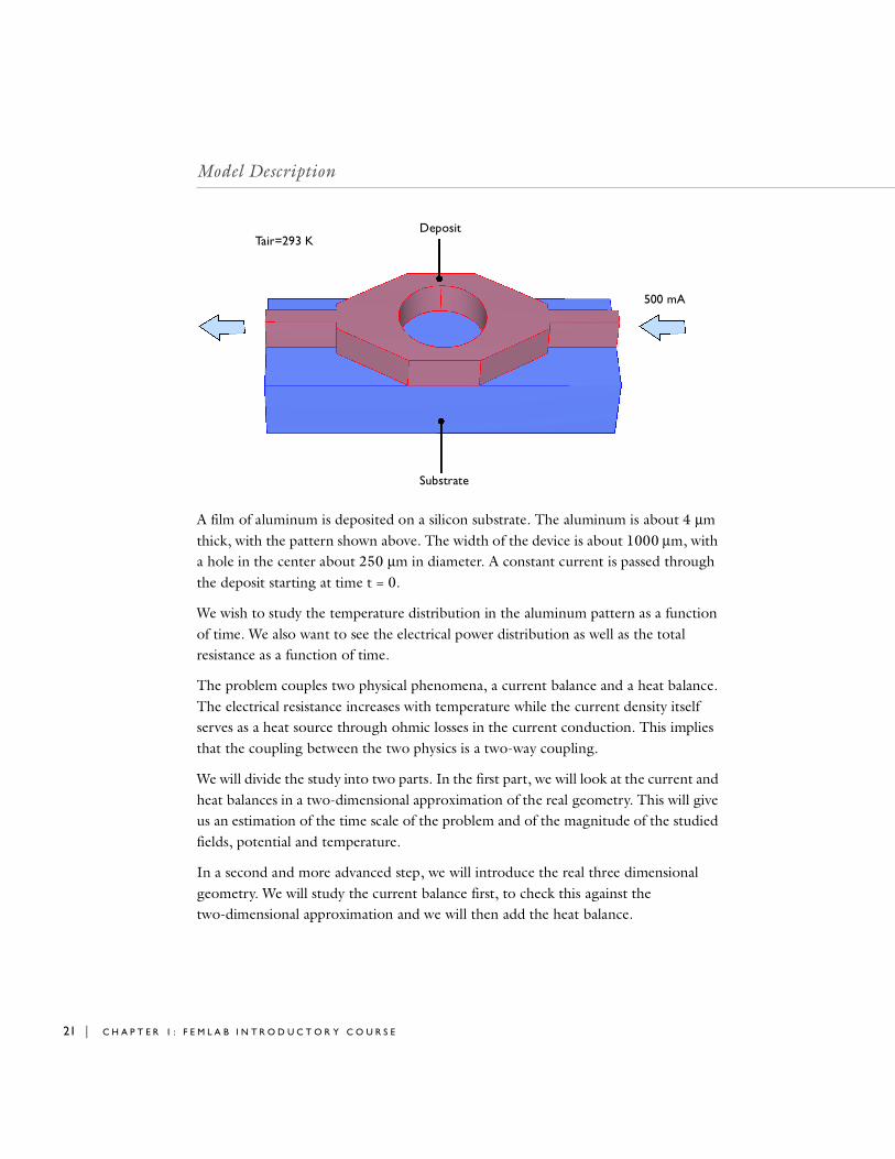
A film of aluminum is deposited on a silicon substrate. The aluminum is about 4 µm thick, with the pattern shown above. The width of the device is about 1000 µm, with a hole in the center about 250 µm in diameter. A constant current is passed through the deposit starting at time t = 0.
We wish to study the temperature distribution in the aluminum pattern as a function of time. We also want to see the electrical power distribution as well as the total resistance as a function of time.
The problem couples two physical phenomena, a current balance and a heat balance. The electrical resistance increases with temperature while the current density itself serves as a heat source through ohmic losses in the current conduction. This implies that the coupling between the two physics is a two-way coupling.
We will divide the study into two parts. In the first part, we will look at the current and heat balances in a two-dimensional approximation of the real geometry. This will give us an estimation of the time scale of the problem and of the magnitude of the studied fields, potential and temperature.
In a second and more advanced step, we will introduce the real three dimensional geometry. We will study the current balance first, to check this against the two-dimensional approximation and we will then add the heat balance.
Tair=293 KDeposit
Substrate
500 mA
C U R R E N T S I N A L U M I N U M D E P O S I T | 22
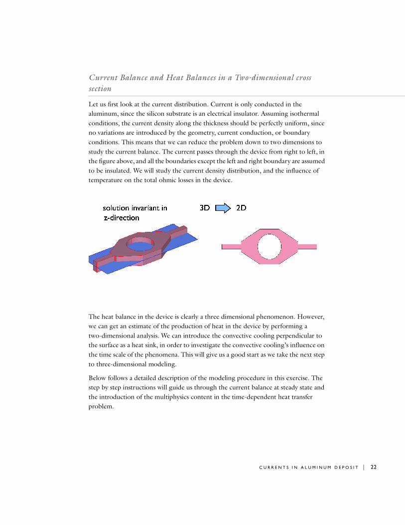
Current Balance and Heat Balances in a Two-dimensional cross section
Let us first look at the current distribution. Current is only conducted in the aluminum, since the silicon substrate is an electrical insulator. Assuming isothermal conditions, the current density along the thickness should be perfectly uniform, since no variations are introduced by the geometry, current conduction, or boundary conditions. This means that we can reduce the problem down to two dimensions to study the current balance. The current passes through the device from right to left, in the figure above, and all the boundaries except the left and right boundary are assumed to be insulated. We will study the current density distribution, and the influence of temperature on the total ohmic losses in the device.
The heat balance in the device is clearly a three dimensional phenomenon. However, we can get an estimate of the production of heat in the device by performing a two-dimensional analysis. We can introduce the convective cooling perpendicular to the surface as a heat sink, in order to investigate the convective cooling’s influence on the time scale of the phenomena. This will give us a good start as we take the next step to three-dimensional modeling.
Below follows a detailed description of the modeling procedure in this exercise. The step by step instructions will guide us through the current balance at steady state and the introduction of the multiphysics content in the time-dependent heat transfer problem.

23 | C H A P T E R 1 : F E M L A B I N T R O D U C T O R Y C O U R S E
Using the Graphical User Interface
1 Start FEMLAB.
2 In the Model Navigator, set Space dimension to 2D and then select FEMLAB>Electromagnetics>Conductive Media DC in the list of available application modes.
Note: Before proceeding, make sure that you have not selected the Electromagnetics
Module branch in the model navigator tree. It should be the FEMLAB branch like described in item 2 above.
3 Click OK.
G E O M E T R Y M O D E L I N G
The second step in the modeling process is to create or import the model geometry. FEMLAB is able to read and repair DXF and IGES files from other solid modeling packages. However, the geometry of the aluminum deposit is very easily created in FEMLAB’s built-in solid modeling tool.
1 Select Axes/Grid Settings in the Options menu.
2 Clear the Axis equal checkbox.

C U R R E N T S I N A L U M I N U M D E P O S I T | 24
3 Type -5.5e-5 in the x min and 1.05e-3 in the x max edit field,
Type -3.5e-4 in the y min and 3.5e-4 in the y max edit field.
4 Click on the Grid tab.
5 Clear the Auto checkbox.
6 Type 1e-4 in the x spacing and y spacing edit fields.
7 Insert extra grid lines by typing -2.5e-5 2.5e-5 5e-5 1.25e-4 1.75e-4 in the Extra y edit field and click OK.
This gives a proper grid spacing for the drawing of the device. You can now start drawing the geometry. The geometry can be created using solid primitive objects or line and curve tools. We will use the line tool to create the main part of the device.
8 Click the Line tool button.
Note: In the following process, you can see the location of the pointer in the bottom left corner of the FEMLAB window.
9 Click on the coordinates tabulated below to create the thick part of the device.
X COORDINATES Y COORDINATES
2e-4 0
2e-4 0.5e-4
4e-4 1.75e-4

25 | C H A P T E R 1 : F E M L A B I N T R O D U C T O R Y C O U R S E
10 Click the right mouse button to create a solid object denoted CO1, composite object 1.
11 Click the Mirror button and specify the reflection line as shown below. Click OK.
6e-4 1.75e-4
8e-4 0.5e-4
8e-4 0
X COORDINATES Y COORDINATES

C U R R E N T S I N A L U M I N U M D E P O S I T | 26
You have created the geometry objects CO1 and CO2 and can continue with FEMLAB’s Create Composite Object button to unify these objects.
12 Select CO1 and CO2 by using the key combination Ctrl+A and click the Create
Composite Object button.
13 Clear the Keep interior boundaries box and click OK.
We will now draw the contact strips to the main body of the device.
14 Click the Rectangle/Square button (top button on the vertical toolbar).
15 Hold down the left mouse button and drag the pointer between the coordinates (0, -0.25e-4) and (1e-3, 0.25e-4) to create a rectangle.
16 Select the rectangle R1 and the composite CO1 (Ctrl+A) and unify them by using the Create Composite Object tool. The Keep interior boundaries box should be cleared.
17 Click OK.
To complete the geometry, create the circle in the middle and drill the hole in the structure.
18 Click the Ellipse/Circle (Centered) button.
19 Using the right mouse button, create a circle by clicking in the center of the geometry (5e-4,0) and dragging upwards until the top of the circle snaps to y=1.25⋅10-4.

27 | C H A P T E R 1 : F E M L A B I N T R O D U C T O R Y C O U R S E
20 Select all the objects by using the key combination Ctrl+A and click the Difference button (seventh button from the bottom on the vertical toolbar).
21 The geometry of the aluminum deposit is completed. This is a good time to go to File, Save As to save your work.
O P T I O N S - C O N S T A N T S
1 Select Constants in the Options menu.
2 Define the constants tabulated below in the corresponding edit fields. sig is a constant that you will use later on to define the electrical conductivity of the material.
3 Click OK.
NAME EXPRESSION DESCRIPTION
iin 0.5 Current (A)
thick 4e-6 Thickness (m)
side 50e-6 Width (m)
sig 3.54e7 Conductivity (Ω-1 m-1)

C U R R E N T S I N A L U M I N U M D E P O S I T | 28
B O U N D A R Y S E T T I N G S
1 Click the Boundary Mode button on the main toolbar.
2 Select all boundaries by using the key combination Ctrl+A.
3 Select Boundary Settings in the Physics menu.
4 Set Electric insulation conditions at all boundaries. Click OK.
5 Double click the rightmost side boundary, boundary 16, and select the Inward
current flow condition from the drop-down list. Type the expressioniin/thick/side in the Jn edit field.
6 Select the left hand side boundary, number 1, and set the Ground boundary condition.
7 Click OK.
This defines the boundary conditions for the current balance. Proceed to the subdomain mode.
S U B D O M A I N S E T T I N G S
1 Click the Subdomain Mode button in the main toolbar.
2 Double-click on the geometry or open Subdomain Settings from the Physics menu and select 1 from the Subdomain Selection list.
3 Type sig in the σ (isotropic) Conductivity edit field.
4 Leave the other fields at the default values (0).
5 Click OK.
The constant sig corresponds to the conductivity, in Ω-1 m-1, at 293 K.
M E S H

29 | C H A P T E R 1 : F E M L A B I N T R O D U C T O R Y C O U R S E
Click the Mesh Mode button in the main toolbar to create the mesh.
C O M P U T I N G T H E S O L U T I O N S
Solve the problem by clicking the Solve button (=) in the main toolbar.
P O S T P R O C E S S I N G
The graphical user interface automatically selects the Postprocessing Mode once the problem is solved. The default plot shows the electric potential in the aluminum deposit.
You can toggle between a number of visualization options by clicking the quick buttons in the Post Mode.
1 Click the Plot Parameters button in the main toolbar.
2 Clear the Surface checkbox and check the Contour checkbox.
3 Select the Contour tab.
Postprocessing modequick buttons
C U R R E N T S I N A L U M I N U M D E P O S I T | 30
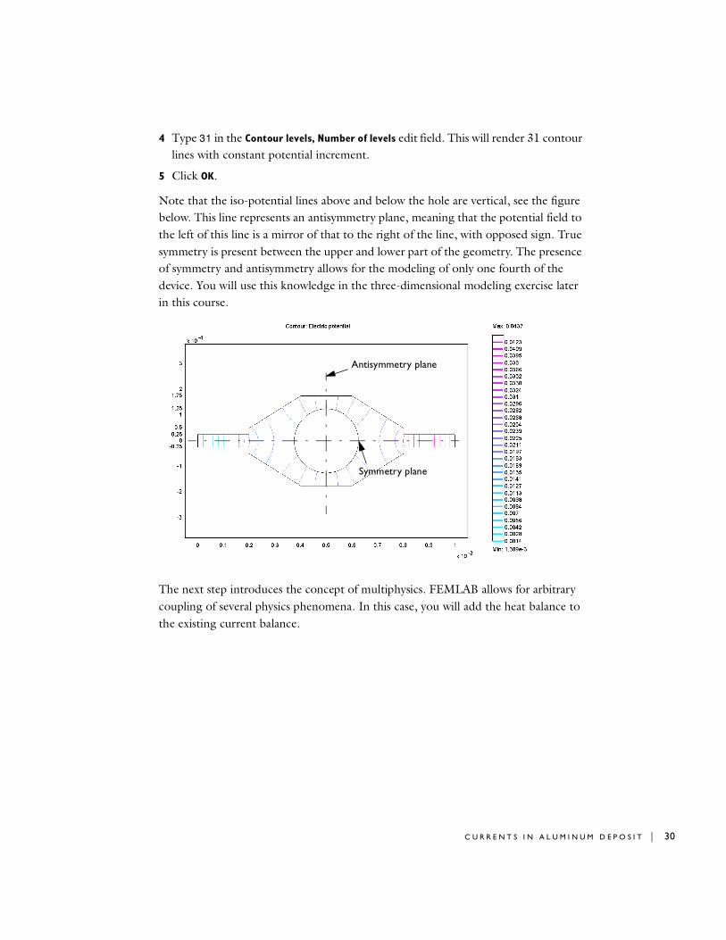
4 Type 31 in the Contour levels, Number of levels edit field. This will render 31 contour lines with constant potential increment.
5 Click OK.
Note that the iso-potential lines above and below the hole are vertical, see the figure below. This line represents an antisymmetry plane, meaning that the potential field to the left of this line is a mirror of that to the right of the line, with opposed sign. True symmetry is present between the upper and lower part of the geometry. The presence of symmetry and antisymmetry allows for the modeling of only one fourth of the device. You will use this knowledge in the three-dimensional modeling exercise later in this course.
The next step introduces the concept of multiphysics. FEMLAB allows for arbitrary coupling of several physics phenomena. In this case, you will add the heat balance to the existing current balance.
Antisymmetry plane
Symmetry plane

31 | C H A P T E R 1 : F E M L A B I N T R O D U C T O R Y C O U R S E
M O D E L N A V I G A T O R
1 Select Model Navigator from the Multiphysics menu.
2 Select FEMLAB>Heat Transfer>Conduction.
3 Click the Add button.
4 Click OK.
Define a few constants, in the temporary data base, for later use.
5 From the Options menu, select Constants.
6 Add to the existing list the constants below.
7 Click OK.
In addition to constants, you can define expressions that are functions of the dependent variables in the model, in this case voltage, V, and temperature T. You can also make expressions of the independent variables x and y, as well as other geometric variables. In the following secti on we will define the expressions described in “Summary of Equations” on page 31.
CONSTANT EXPRESSION DESCRIPTION
ro1 2.7e3 Density (kg m-3)
cp1 900 Heat capacity (J kg-1 K-1)
k1 240 Thermal conductivity (W m-1 K-1)
h1 5 Heat transfer coefficient (W m-2 K-1)
Tinf 293 Reference temperature (K)

C U R R E N T S I N A L U M I N U M D E P O S I T | 32
1 Select Expressions/Scalar Expressions in the Options menu.
2 Define the following expression for the resistivity (Ω m).
Make sure that you do not leave spaces when you enter the expression. FEMLAB interprets spaces as separation between the components of a vector.
3 Click OK.
B O U N D A R Y S E T T I N G S
1 Click the Boundary Mode button.
2 Select all boundaries by pressing Ctrl+A.
3 Select Boundary Settings in the Physics menu.
4 Select Heat flux from the Boundary condition drop down list.
5 Type h1 in the Heat transfer coefficient edit field.
6 Type Tinf in the External temperature edit field.
7 In the boundary selection list, make sure that only boundaries 1 and 16 are highlighted. You can do this by holding down the Ctrl key and pointing directly on the boundaries in the drawing of the device.
8 Select Temperature from the Boundary condition drop down list and type Tinf in the Temperature edit field.
9 Click OK.
You will now continue by defining the domain physics for the heat transfer mode.
NAME EXPRESSION
res 2.824e-8*(1+3.9e-5*(T-Tinf))

33 | C H A P T E R 1 : F E M L A B I N T R O D U C T O R Y C O U R S E
S U B D O M A I N S E T T I N G S
1 Click the Subdomain Mode button.
2 Double-click on the domain drawing.
3 Define the Subdomain Settings according to the table below.
Q_dc is called a postprocessing variable and is predefined in the conductive media application mode as the resistive heating (W m-3). You can check the definition of Q_dc by selecting the menu Physics/Equation System/Subdomain Settings, Variables tab. This way you can verify that it represents σ|∇V|2, see “Summary of Equations” on page 31.
4 Click the Init tab and type Tinf in the Initial value edit field.
5 Click OK.
6 Select Conductive Media DC (dc) in the Multiphysics menu.
DESCRIPTION VALUE
Thermal conductivity k1
Density ro1
Heat capacity cp1
Heat source Q_dc
Convective heat transfer coefficient h1/thick
External temperature Tinf

C U R R E N T S I N A L U M I N U M D E P O S I T | 34
7 Select Subdomain Settings in the Physics menu.
8 Replace sig with 1/res in the Conductivity edit field.
9 Click OK.
Note that the heat transfer through convection on the surface of the aluminum deposit is introduced as a source or sink. Since symmetry along the thickness of the device implies that the model is defined per unit length perpendicular to the paper, the heat transfer coefficient has to be divided by the thickness of the deposit. This gives the correct value of the cooling per unit volume of aluminum. The coupling between the heat balance and the current balance is here present in the expression for the resistivity, denoted res, and the source term, which depends on the gradients of the potential, terms denoted Vx and Vy.
In order to make a two-way coupling between the heat and current balances, you have to introduce the expression for the resistivity, res, in the conductive media application.
Heat transfer is a phenomenon that takes place in a much greater time scale than current transfer. In comparing the two phenomena, current density can be assumed to respond immediately to a change in potential. You can therefore assume that the current balance is always a steady-state problem, while the heat balance remains a transient problem.
C O M P U T I N G T H E S O L U T I O N
1 Select Solver Parameters in the Solve menu.
2 Select Solver: Time dependent in the left list on the General tab.

35 | C H A P T E R 1 : F E M L A B I N T R O D U C T O R Y C O U R S E
3 Type 0:0.001:0.03 in the Times edit field.
4 Select Solution form: General and click OK.
5 Click the Solve button.
The vector expression for the output times gives the solution from 0 to 0.03 seconds with 0.001 second increments. The time stepping algorithm has built-in step length control and the output time only defines the steps that should be saved for post processing.
You have already solved the potential field at 293 K, which corresponds to the initial condition on the temperature. If we now assign this calculated potential field as the initial condition for the time dependent problem, there is perfect consistency in the initial conditions, which gives an excellent start for the time dependent solver. Well posed initial conditions are very important in coupled systems of stationary and time dependent problems (DAE-systems). FEMLAB provides a fully automatic procedure to get consistent initial conditions for a DAE systems. This is accomplished by setting Consistent initialization of DAE systems: On on the Timestepping page of the Solver
Parameters dialog box. This will generate perturbed initial solution (t=0) of the stationary equation (potential field), but the problem will be well-posed.
C U R R E N T S I N A L U M I N U M D E P O S I T | 36
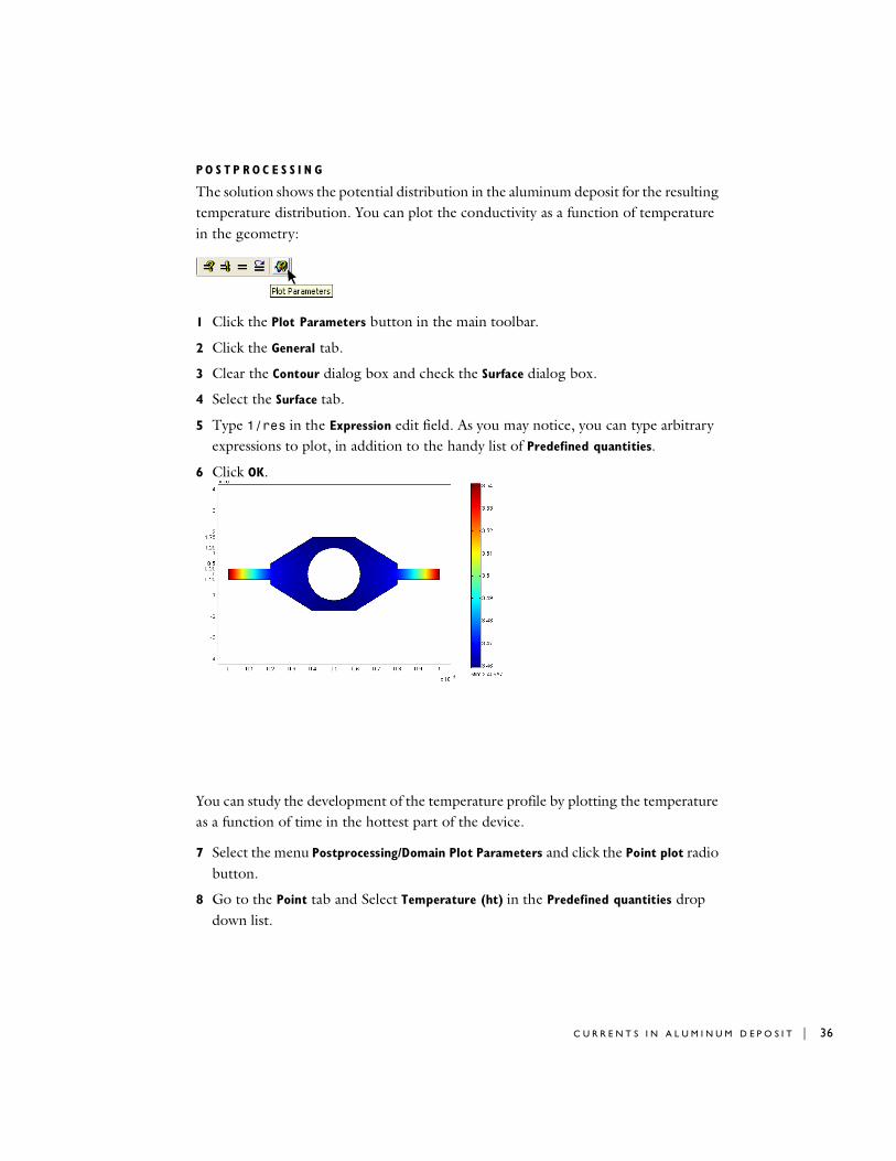
P O S T P R O C E S S I N G
The solution shows the potential distribution in the aluminum deposit for the resulting temperature distribution. You can plot the conductivity as a function of temperature in the geometry:
1 Click the Plot Parameters button in the main toolbar.
2 Click the General tab.
3 Clear the Contour dialog box and check the Surface dialog box.
4 Select the Surface tab.
5 Type 1/res in the Expression edit field. As you may notice, you can type arbitrary expressions to plot, in addition to the handy list of Predefined quantities.
6 Click OK.
You can study the development of the temperature profile by plotting the temperature as a function of time in the hottest part of the device.
7 Select the menu Postprocessing/Domain Plot Parameters and click the Point plot radio button.
8 Go to the Point tab and Select Temperature (ht) in the Predefined quantities drop down list.

37 | C H A P T E R 1 : F E M L A B I N T R O D U C T O R Y C O U R S E
9 Select point 11 from the Point selection list and Click OK.
Figure 1-1: Time evolution of the temperature at a point.
The resulting plot shows that the problem has reached steady-state after 0.02 seconds. You can continue visualizing the current density, potential, and current density distribution by combining cross sectional, surface, contours, and flow plots.
10 You can save that data in a text file by clicking the ASCII button in the separate figure window.
More advanced data export is possible to do in the main GUI as well as by selecting the File/Export/Postprocessing Data menu item.
Convergence analysis (optional)
To check the numerical accuracy of the solutions, we need to examine the sensitivity of the values to the mesh density. We will look at a key number in the solution at the

C U R R E N T S I N A L U M I N U M D E P O S I T | 38
end time and compare them at different mesh densities. The integral mean temperature can be defined as
and we will look at this quantity during the convergence analysis.
1 Change to a stationary problem by selecting the Solve/Solver Parameters menu and select Solver to Stationary nonlinear. Click OK to close the dialog box.
2 Create two scalar coupling variables by selecting the menu Options/Integration
Coupling Variables/Subdomain Variables. Select subdomain 1 and define the list according to the table below. Click OK.
3 Solve the problem by clicking the = button.
4 To evaluate the mean temperature, click the Plot Parameters button and enter Tint/A1 in the expression field of the Surface tab. Click OK. You can see the numerical value in the status field by clicking inside the domain on the drawing board.
5 Repeat the above point for different mesh sizes. For each mesh size in the table below, open the menu item Mesh/Mesh Parameters. Go to the Subdomain tab and enter the mesh size in the Maximum element size dialog box. Click OK and the Initialize Mesh button to see the new mesh. Solve and plot. Fill out the mean temperature values in the table.
You will see that the mean value of the temperature will eventually converge toward a certain value. When you are satisfied with the relative deviation between two refinements, you have a mesh that is sufficiently fine. Bear in mind that there might be other quantities you will want to check, for example a total flux or heat balance.
NAME EXPRESSION INTEGRATION ORDER DESTINATION
Tint T 4 global
A1 1 4 global
MAXIMUM MESH ELEMENT SIZE <T>
3e-5 326.138
1.5e-5 326.219
0.75e-5 326.254
T⟨ ⟩ T A A⁄d∫=

39 | C H A P T E R 1 : F E M L A B I N T R O D U C T O R Y C O U R S E
The Three-Dimensional Current and Heat Balances
The real device is actually three-dimensional where the heating introduces three-dimensional effects. Current heats the aluminum where heat is then dissipated to the adjacent air and to the silicon substrate. For this reason, there will be a temperature gradient along the thickness of the aluminum plate, which impedes us from reducing the problem to two space dimensions. In this study, we will make use of the symmetry and antisymmetry in the problem to reduce the geometry to one fourth of the original description. We will only solve the stationary problem.
The boundary conditions and the expression for the conductivity are identical in the 2D and 3D problems for current conduction. This implies electrical insulation everywhere except for the edges on the right and left.
The heat balance is a little more difficult to define. Temperature is fixed on the right and left edges of the device. On the base of the silicon substrate and at the vertical boundaries of the substrate, we assume thermal insulation. At all other surfaces, we define convective heat dissipation using the film theory, where tabulated values for the heat transfer coefficient are used. At the boundary between the aluminum film and the substrate, FEMLAB automatically gives the continuity in temperature and heat flux.
The next step is to define the heat balance in the device. In the silicon substrate, only conduction and the accumulation of heat takes place. This is also the case for the aluminum film, where heat generation is also introduced by the conduction of current, which is proportional to the square of the current density.

C U R R E N T S I N A L U M I N U M D E P O S I T | 40
The thickness and length of the device geometry differ by several orders of magnitude. This implies that a large number of elements would be required if we treated the problem without any type of scaling, since the smallest length would determine the edge size of the elements. Therefore, we will use an anisotropic mesh by scaling the geometry in the thickness direction prior to meshing. FEMLAB will automatically scale it back for viewing.
Creating the 3D Model Geometry
Save the 2D model in a file such as, intro2d.fl. Now, do Save as...intro3d.fl.
Let us start by creating the three dimensional geometry by using the existing geometry as starting point.
1 Remove the left and the lower half of the geometry by drawing suitable rectangles and subtracting them from the geometry by using the Create Composite Object button. Start by clicking the Draw Mode button. To draw the rectangles, press Ctrl+A and click the Create Composite Object to perform the suitable operations.
2 Click the Zoom Extents button.
The cross-sectional geometry is now one fourth of the original. Create the rectangular cross-section of the substrate.
3 Click the Rectangle/Square button.
41 | C H A P T E R 1 : F E M L A B I N T R O D U C T O R Y C O U R S E
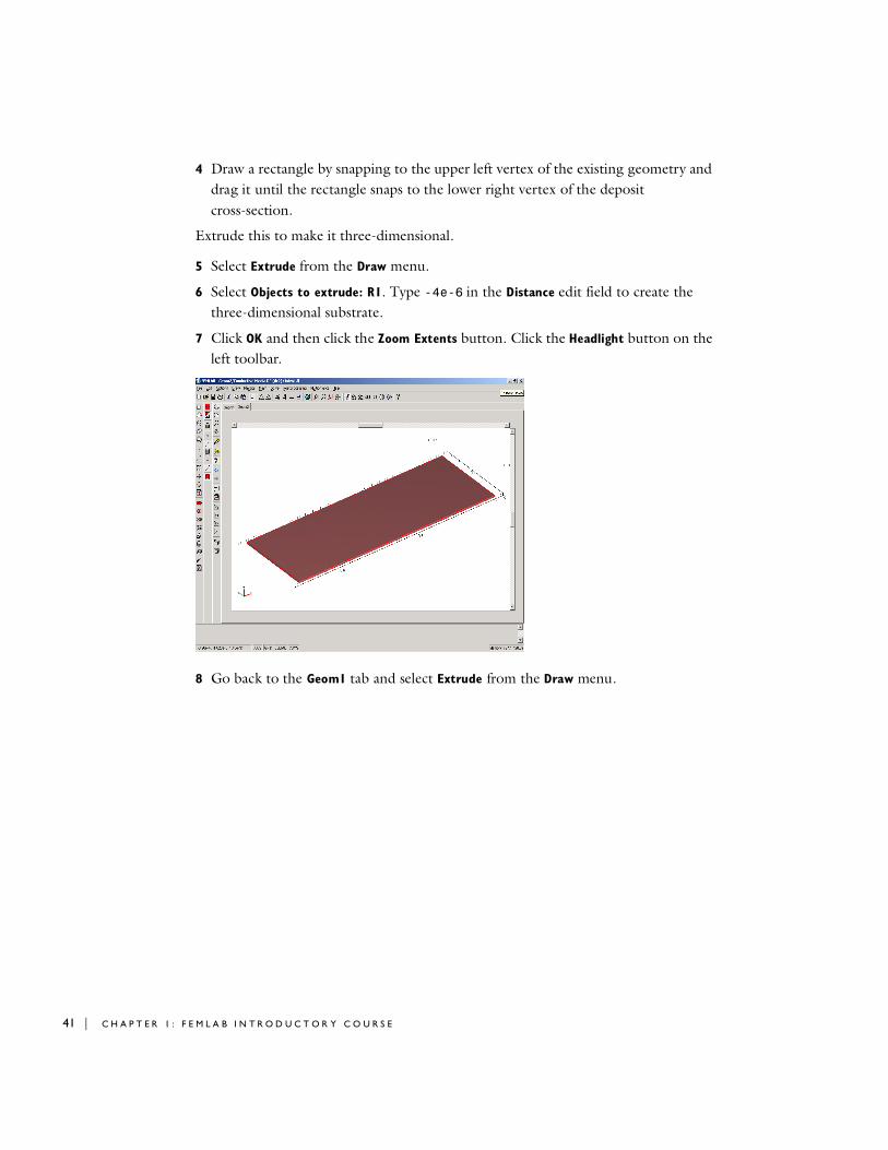
4 Draw a rectangle by snapping to the upper left vertex of the existing geometry and drag it until the rectangle snaps to the lower right vertex of the deposit cross-section.
Extrude this to make it three-dimensional.
5 Select Extrude from the Draw menu.
6 Select Objects to extrude: R1. Type -4e-6 in the Distance edit field to create the three-dimensional substrate.
7 Click OK and then click the Zoom Extents button. Click the Headlight button on the left toolbar.
8 Go back to the Geom1 tab and select Extrude from the Draw menu.

C U R R E N T S I N A L U M I N U M D E P O S I T | 42
9 Select Objects to extrude: CO1. Type 3e-6 in the Distance edit field, click OK.
O P T I O N S
1 Select Constants from the Options menu and add additional input data to the existing table. See the table below:
2 Click OK.
S U B D O M A I N S E T T I N G S
1 Select the Model Navigator item from the Multiphysics menu. Highlight Geom2 in the right pane. Select FEMLAB>Electromagnetics>Conductive Media DC in the left pane and click Add.
2 Select FEMLAB>Heat Transfer>Conduction and click Add. Click OK.
3 Select Geom2: Conductive Media DC (dc2) in the Multiphysics Menu.
4 Select the menu Options>Constants and remove the entry sig and its expression in the constant list. Click OK. The empty row should now have disappeared.
CONSTANT NAME EXPRESSION
L 0.05
cp2 778
k2 84
ro2 2330
43 | C H A P T E R 1 : F E M L A B I N T R O D U C T O R Y C O U R S E
5 Select Expressions/Scalar Expressions from the Options menu and add the following expressions.
6 Click OK.
You can now define the current balance.
7 Select Multiphysics/ 3 Geom2: Conductive Media DC (dc2). Select Subdomain Settings in the Physics menu.
8 Select subdomain 1, corresponding to the substrate, and clear the Active in this
domain checkbox.
This deactivates the current balance in the substrate, since the substrate does not conduct current.
9 Select subdomain 2 and type sig in σ (isotropic) Conductivity edit field. Use the default 0 in the Current source and External current density edit fields.
10 Click OK.
Toggle to the Heat Transfer by Conduction (ht2) application mode to define the subdomain settings.
11 Select Geom2: Heat Transfer by Conduction (ht2) in the Multiphysics menu.
12 Select subdomain 1 and define the Subdomain Settings according to following table.
13 Under the Init tab, set the initial condition to Tinf.
14 Select subdomain 2 and define the Subdomain Settings according to the table below:
VARIABLES DEFINITION
res 2.824e-8*(1+3.9e-5*(T2-293))
sig 1/res
DESCRIPTION VALUE
Thermal conductivity (isotropic) k2
Density ro2
Heat capacity cp2
Heat source 0
DESCRIPTION VALUE
Thermal conductivity (isotropic) k1
Density ro1
C U R R E N T S I N A L U M I N U M D E P O S I T | 44
15 Under the Init tab, set the initial condition to Tinf.
16 Click OK.
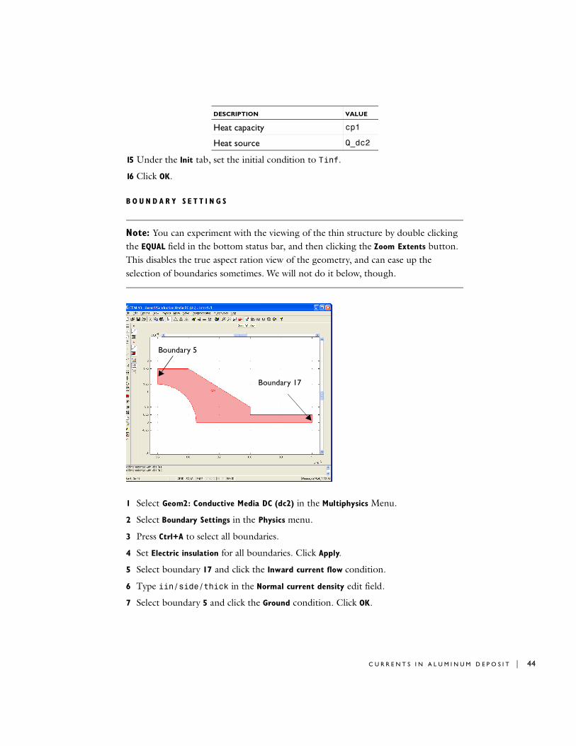
B O U N D A R Y S E T T I N G S
Note: You can experiment with the viewing of the thin structure by double clicking the EQUAL field in the bottom status bar, and then clicking the Zoom Extents button. This disables the true aspect ration view of the geometry, and can ease up the selection of boundaries sometimes. We will not do it below, though.
1 Select Geom2: Conductive Media DC (dc2) in the Multiphysics Menu.
2 Select Boundary Settings in the Physics menu.
3 Press Ctrl+A to select all boundaries.
4 Set Electric insulation for all boundaries. Click Apply.
5 Select boundary 17 and click the Inward current flow condition.
6 Type iin/side/thick in the Normal current density edit field.
7 Select boundary 5 and click the Ground condition. Click OK.
Heat capacity cp1
Heat source Q_dc2
DESCRIPTION VALUE
Boundary 5
Boundary 17

45 | C H A P T E R 1 : F E M L A B I N T R O D U C T O R Y C O U R S E
8 Select Geom2: Heat Transfer by Conduction (ht2) in the Multiphysics Menu.
9 Select Boundary Settings in the Physics menu.
10 Click Ctrl+A to select all boundaries.
11 Set Thermal insulation for all boundaries.
12 Select boundaries 4, 6, 8, 10, 11, 12, 14, and 15. You can select the boundaries by clicking once on a boundary to color it red. Then right-click to lock the selection (the boundary turns blue). Then select the next boundary.
13 Set Heat flux for the boundaries and type h1 in the Heat transfer coefficient edit field and Tinf in the External temperature edit field.
14 Select boundary 17 (far end of coating).
15 Select the Temperature condition and type Tinf in the corresponding edit field.
16 Click OK.
C R E A T I N G T H E M E S H
1 Open the Mesh Parameters window from the Mesh menu.
2 Click the Advanced tab.
3 Set z-direction scale factor to 7. Let the scale factors in the x and y directions remain default 1.
4 Press the Remesh button. Close the window by pressing OK.
C O M P U T I N G T H E S O L U T I O N
1 Click the Solver Manager button.

C U R R E N T S I N A L U M I N U M D E P O S I T | 46
2 Go to the Solve For tab and select only the Geom2 equations (Ctrl- click). See figure below. Click OK.
3 Click the Solver Parameters button. On the General tab, select the Solver: Stationary
nonlinear, as well as the Solution form: General option. Click OK.
4 Click the Solve button.
T I M E D E P E N D E N T S I M U L A T I O N
5 Click the Solver Parameters button. On the General tab, select the Solver: Time
dependent. Click OK.
6 Click the Solve button.
P O S T P R O C E S S I N G
1 Click the Plot Parameters button.
2 Check the Isosurface and Boundary and Geometry edges checkboxes and select the Isosurface tab.
3 Select Temperature (ht2) from the Predefined quantities list. Enter 20 in the Number
of levels field. Finally, select Colormap: jet.
4 Go to the Boundary tab and select Temperature (ht2) as the Predefined quantity. Select Colormap: gray. Click OK.

47 | C H A P T E R 1 : F E M L A B I N T R O D U C T O R Y C O U R S E
5 Select menu Options/Suppress/Suppress Boundaries. Ctrl-click boundaries 4, 8 and 12. Click OK.
6 Click the Postprocessing Mode button.
7 Click the Headlight button to switch of the lighting.
Continue experimenting with the postprocessing variables to study he distribution of the source, conductivity, current distribution with time, etc. Work with the Domain plot parameters and cross section plots.
Summary of Equations
The equations in this example would be very useful in completely defining our problem mathematically. But by using FEMLAB they are not required in our exercise and they are definitely not required to understand the physics in our problem. The mathematical equations express the problem in a precise and compact way. It would be tedious to have to explain the equations in words but in the mathematical language they can be written in a few lines.
The current balance in the aluminum deposit is given by:

C U R R E N T S I N A L U M I N U M D E P O S I T | 48
where σ is a function of temperature according to:
The boundary conditions for the current balance are insulating conditions except for the right and left boundaries of the aluminum deposit. The insulating boundaries are expressed by:
At the inlet of the current, the boundary condition reads:
while the outlet is defined by:
The heat transfer equations are also based on flux balances but this time the time dependence is introduced:
In the silicon substrate, the following equation is valid:
The convective boundary conditions are given by the expression below for both aluminum and substrate:
The insulating conditions are obtained through
and the temperature conditions are set by
∇ σ V∇–( )⋅ 0=
σ 1a 1 b T T0–( )+( )-------------------------------------------=
σ V∇–( ) n⋅ 0=
σ V∇–( ) n⋅ j0=
V V0=
ρCp∂T∂t------- ∇+ k T∇–( )⋅ σ V∇ 2
=
ρCp∂T∂t------- ∇+ k T∇–( )⋅ 0=
k T∇–( ) n⋅ h T T0–( )=
k T∇–( ) n⋅ 0=
T T0=

49 | C H A P T E R 1 : F E M L A B I N T R O D U C T O R Y C O U R S E
The thermal conductivity, k, density, ρ, and heat capacity, Cp, have different values in the deposit and the substrate.