MIDAS in gretl

Allin Cottrell, Jack Lucchetti

September 19, 2017

These notes describes the state of play with regard to MIDAS (Mixed Data Sampling—see Ghy-sels et al., 2004; Ghysels, 2015; Armesto et al., 2010) in gretl as of the 2017a release (March2017). The points covered in these notes are not yet elaborated in the formal gretl docu-mentation, but the relevant new commands and functions are described in the current GretlCommand Reference.

1 Handling data of more than one frequency

The essential move in MIDAS is estimation of models including one or more independentvariables observed at a higher frequency than the dependent variable. Since a gretl datasetformally handles only a single data frequency it may seem that we have a problem. However,we have adopted a straightforward solution: a higher frequency series xH is represented by aset of m series, each holding the value of xH in a sub-period of the “base” (lower-frequency)period (where m is the ratio of the higher frequency to the lower).

This is most easily understood by means of an example. Suppose our base frequency is quar-terly and we wish to include a monthly series in the analysis. Then a relevant fragment of thegretl dataset might look as shown in Table 1. Here, gdpc96 is a quarterly series while indprois monthly, so m = 12/4 = 3 and the per-month values of indpro are identified by the suffix_mn, n = 3,2,1.

gdpc96 indpro_m3 indpro_m2 indpro_m1

1947:1 1934.47 14.3650 14.2811 14.19731947:2 1932.28 14.3091 14.3091 14.25321947:3 1930.31 14.4209 14.3091 14.22531947:4 1960.70 14.8121 14.7562 14.56061948:1 1989.54 14.7563 14.9240 14.89601948:2 2021.85 15.2313 15.0357 14.7842

Table 1: A slice of MIDAS data

To recover the actual monthly time series for indpro one must read the three relevant seriesright-to-left by row. At first glance this may seem perverse, but in fact it is the most convenientsetup for MIDAS analysis. In such models, the high-frequency variables are represented bylists of lags, and of course in econometrics it is standard to give the most recent lag first(xt−1, xt−2, . . .).

One can construct such a dataset manually from “raw” sources using hansl’s matrix-handlingmethods or the join command (see Appendix A for illustrations), but we have added native

1

support for the common cases shown below.

base frequency higher frequency

annual quarterly or monthly

quarterly monthly or daily

monthly daily

The examples below mostly pertain to the case of quarterly plus monthly data. Appendix Bhas details on our handling of daily data.

The new native methods support creation of a MIDAS-ready dataset in either of two ways:by selective importation of series from a database, or by creating two datasets of differentfrequencies then merging them.

Importation from a database

Here’s a simple example, in which we draw from the fedstl (St Louis Fed) database which issupplied in the gretl distribution:

clearopen fedstl.bindata gdpc96data indpro --compact=spreadstore gdp_indpro.gdt

Since gdpc96 is a quarterly series, its importation via the data command establishes a quar-terly dataset. Then the MIDAS work is done by the option --compact=spread for the secondinvocation of data. This “spreads” the series indpro—which is monthly at source—into threequarterly series, exactly as shown in Table 1.

Merging two datasets

In this case we consider an Excel file provided by Eric Ghysels in his MIDAS Matlab Toolbox,1

namely mydata.xlsx. This contains quarterly real GDP in Sheet1 and monthly non-farm pay-roll employment in Sheet2. A hansl script to build a MIDAS-style file named gdp_midas.gdtis shown in Listing 1.

Note that both series are simply named VALUE in the source file, so we use gretl’s renamecommand to set distinct and meaningful names. The heavy lifting is done here by the line

dataset compact 4 spread

which tells gretl to compact an entire dataset (in this case, as it happens, just containing oneseries) to quarterly frequency using the “spread” method. Once this is done, it is straightfor-ward to append the compacted data to the quarterly GDP dataset.

We will put this dataset to use in subsequent sections. Note that it is provided in the gretlpackage (gdp_midas, which you can find under the Gretl tab in the practice datafiles windowin the gretl GUI).

1See http://www.unc.edu/~eghysels/ for links.

2

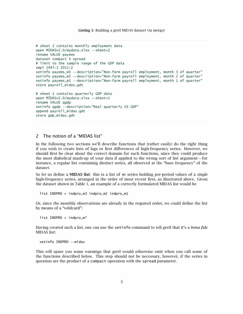
Listing 1: Building a gretl MIDAS dataset via merger

# sheet 2 contains monthly employment dataopen MIDASv2.0/mydata.xlsx --sheet=2rename VALUE payemsdataset compact 4 spread# limit to the sample range of the GDP datasmpl 1947:1 2011:2setinfo payems_m3 --description="Non-farm payroll employment, month 3 of quarter"setinfo payems_m2 --description="Non-farm payroll employment, month 2 of quarter"setinfo payems_m1 --description="Non-farm payroll employment, month 1 of quarter"store payroll_midas.gdt

# sheet 1 contains quarterly GDP dataopen MIDASv2.0/mydata.xlsx --sheet=1rename VALUE qgdpsetinfo qgdp --description="Real quarterly US GDP"append payroll_midas.gdtstore gdp_midas.gdt

2 The notion of a “MIDAS list”

In the following two sections we’ll describe functions that (rather easily) do the right thingif you wish to create lists of lags or first differences of high-frequency series. However, weshould first be clear about the correct domain for such functions, since they could producethe most diabolical mash-up of your data if applied to the wrong sort of list argument—forinstance, a regular list containing distinct series, all observed at the “base frequency” of thedataset.

So let us define a MIDAS list: this is a list of m series holding per-period values of a singlehigh-frequency series, arranged in the order of most recent first, as illustrated above. Giventhe dataset shown in Table 1, an example of a correctly formulated MIDAS list would be

list INDPRO = indpro_m3 indpro_m2 indpro_m1

Or, since the monthly observations are already in the required order, we could define the listby means of a “wildcard”:

list INDPRO = indpro_m*

Having created such a list, one can use the setinfo command to tell gretl that it’s a bona fideMIDAS list:

setinfo INDPRO --midas

This will spare you some warnings that gretl would otherwise emit when you call some ofthe functions described below. This step should not be necessary, however, if the series inquestion are the product of a compact operation with the spread parameter.

3

Inspecting high-frequency data

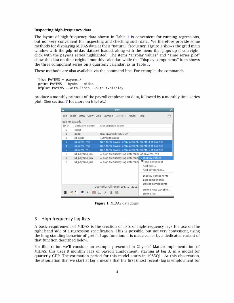
The layout of high-frequency data shown in Table 1 is convenient for running regressions,but not very convenient for inspecting and checking such data. We therefore provide somemethods for displaying MIDAS data at their “natural” frequency. Figure 1 shows the gretl mainwindow with the gdp_midas dataset loaded, along with the menu that pops up if you right-click with the payems series highlighted. The items “Display values” and “Time series plot”show the data on their original monthly calendar, while the “Display components” item showsthe three component series on a quarterly calendar, as in Table 1.

These methods are also available via the command line. For example, the commands

list PAYEMS = payems_*print PAYEMS --byobs --midashfplot PAYEMS --with-lines --output=display

produce a monthly printout of the payroll employment data, followed by a monthly time-seriesplot. (See section 7 for more on hfplot.)

Figure 1: MIDAS data menu

3 High-frequency lag lists

A basic requirement of MIDAS is the creation of lists of high-frequency lags for use on theright-hand side of a regression specification. This is possible, but not very convenient, usingthe long-standing behavior of gretl’s lags function; it is made easier by a dedicated variant ofthat function described below.

For illustration we’ll consider an example presented in Ghysels’ Matlab implementation ofMIDAS: this uses 9 monthly lags of payroll employment, starting at lag 3, in a model forquarterly GDP. The estimation period for this model starts in 1985Q1. At this observation,the stipulation that we start at lag 3 means that the first (most recent) lag is employment for

4

October 1984,2 and the 9-lag window means that we need to include monthly lags back toFebruary 1984. Let the per-month employment series be called x_m3, x_m2 and x_m1, and let(quarterly) lags be represented by (-1), (-2) and so on. Then the terms we want are (readingleft-to-right by row):

. . x_m1(-1)

x_m3(-2) x_m2(-2) x_m1(-2)

x_m3(-3) x_m2(-3) x_m1(-3)

x_m3(-4) x_m2(-4) .

We could construct such a list in gretl using the following standard syntax. (Note that the thirdargument of 1 to lags below tells gretl that we want the terms ordered “by lag” rather than“by variable”; this is required to respect the order of the terms shown above.)

list X = x_m*# create lags for 4 quarters, "by lag"list XL = lags(4,X,1)# convert the list to a matrixmatrix tmp = XL# trim off the first two elements, and the lasttmp = tmp[3:11]# and convert back to a listXL = tmp

However, the following specialized syntax is more convenient:

list X = x_m*setinfo X --midas# create high-frequency lags 3 to 11list XL = hflags(3, 11, X)

In the case of hflags the length of the list given as the third argument defines the “compactionratio” (m = 3 in this example); we can (in fact, must) specify the lags we want in high-frequencyterms; and ordering of the generated series by lag is automatic.

Word to the wise: do not use hflags on anything other than a MIDAS list as defined insection 2, unless perhaps you have some special project in mind and really know what you aredoing.

Leads and nowcasting

Before leaving the topic of lags, it is worth commenting on the question of leads and so-called“nowcasting”—that is, prediction of the current value of a lower-frequency variable before itsmeasurement becomes available.

In a regular dataset where all series are of the same frequency, lag 1 means the observationfrom the previous period, lag 0 is equivalent to the current observation, and lag −1 (or lead 1)is the observation for the next period into the relative future.

When considering high-frequency lags in the MIDAS context, however, there is no uniquely de-termined high-frequency sub-period which is temporally coincident with a given low-frequency

2That is what Ghysels means, but see the sub-section on “Leads and nowcasting” below for a possible ambiguityin this regard.

5

period. The placement of high-frequency lag 0 therefore has to be a matter of convention. Un-fortunately, there are two incompatible conventions in currently available MIDAS software, asfollows.

• High-frequency lag 0 corresponds to the first sub-period within the current low-frequencyperiod. This is what we find in Eric Ghysels’ MIDAS Matlab Toolbox; it’s also clearly statedand explained in Armesto et al. (2010).

• High-frequency lag 0 corresponds to the last sub-period in the current low-frequencyperiod. This convention is employed in the midasr package for R.3

Consider, for example, the quarterly/monthly case. In Matlab, high-frequency (HF) lag 0 is thefirst month of the current quarter, HF lag 1 is the last month of the prior quarter, and so on. Inmidasr, however, HF lag 0 is the last month of the current quarter, HF lag 1 the middle monthof the quarter, and HF lag 3 is the first one to take you “back in time” relative to the start ofthe current quarter, namely to the last month of the prior quarter.

In gretl we have chosen to employ the first of these conventions. So Lag 1 points to the mostrecent sub-period in the previous base-frequency period, lag 0 points to the first sub-period inthe current period, and lag −1 to the second sub-period within the current period. Continuingwith the quarterly/monthly case, monthly observations for lags 0 and −1 are likely to becomeavailable before a measurement for the quarterly variable is published (possibly also a monthlyvalue for lag −2). The first “truly future” lead does not occur until lag −3.

The hflags function supports negative lags. Suppose one wanted to use 9 lags of a high-frequency variable, −1,0,1, . . . ,7, for nowcasting. Given a suitable MIDAS list, X, the followingwould do the job:

list XLnow = hflags(-1, 7, X)

This means that one could generate a forecast for the current low-frequency period (which isnot yet completed and for which no observation is available) using data from two sub-periodsinto the low-frequency period (e.g. the first two months of the quarter).

4 High-frequency first differences

When working with non-stationary data one may wish to take first differences, and in theMIDAS context that probably means high-frequency differences of the high-frequency data.Note that the ordinary gretl functions diff and ldiff will not do what is wanted for seriessuch as indpro, as shown in Table 1: these functions will give per-month quarterly differencesof the data (month 3 of the current quarter minus month 3 of the previous quarter, and so on).

To get the desired result one could create the differences before compacting the high-frequencydata but this may not be convenient, and it’s not compatible with the method of constructinga MIDAS dataset shown in section 1. The alternative is to employ the specialized differencingfunction hfdiff. This takes one required argument, a MIDAS list as defined in section 2. Asecond, optional argument is a scalar multiplier (with default value 1.0); this permits scalingthe output series by a constant. There’s also an hfldiff function for creating high-frequencylog differences; this has the same syntax as hfdiff.

So for example, the following creates a list of high-frequency percentage changes (100 timeslog-difference) then a list of high-frequency lags of the changes.

3See http://cran.r-project.org/web/packages/midasr/, and for documentation https://github.com/mpiktas/midasr-user-guide/raw/master/midasr-user-guide.pdf.

6

list X = indpro_*setinfo X --midaslist dX = hfldiff(X, 100)list dXL = hflags(3, 11, dX)

If you only need the series in the list dXL, however, you can nest these two function calls:

list dXL = hflags(3, 11, hfldiff(X, 100))

5 Parsimonious parameterizations

The simplest MIDAS regression specification—known as “unrestricted MIDAS” or U-MIDAS—simply includes p lags of a high-frequency regressor, each with its own parameter to be es-timated (which can be done via OLS). It is more common, however, to enforce parsimony bymaking the individual coefficients on lagged high-frequency terms a function of a relativelysmall number of hyperparameters. This presents a couple of computational questions: howto calculate the per-lag coefficients given the values of the hyperparameters, and how best toestimate the value of the hyperparameters?

Hansl is functional enough to allow a savvy user to address these questions from scratch,but of course it’s helpful to have some built-in high-level functionality. At present gretl canhandle natively four commonly used parameterizations: normalized exponential Almon, nor-malized beta (with or without a zero last coefficient) and plain (non-normalized) Almon poly-nomial. The Almon variants take one or more parameters (two being a common choice), andthe beta takes either two or three parameters.4 All are handled by the functions mweights andmgradient. These functions work as follows.

• mweights takes three arguments: the number of lags required (p), the k-vector of hy-perparameters (θ), and an integer code or string indicating the method (see Table 2). Itreturns a p-vector containing the coefficients.

• mgradient takes three arguments, just like mweights. However, this function returns ap×kmatrix holding the (analytical) gradient of the p coefficients or weights with respectto the k elements of θ.

Parameterization code string

Normalized exponential Almon 1 "nealmon"

Normalized beta, zero last lag 2 "beta0"

Normalized beta, non-zero last lag 3 "betan"

Almon polynomial 4 "almonp"

Table 2: MIDAS parameterizations

An additional function is provided for convenience: it is named mlincomb and it combinesmweights with the long-standing lincomb function, which takes a list (of series) argumentfollowed by a vector of coefficients and produces a series result, namely a linear combinationof the elements of the list. If we have a suitable list L available, we can do, for example,

series foo = mlincomb(L, theta, "beta0")

4Two is the standard case; see Appendix C for details.

7

This is equivalent to

series foo = lincomb(L, mweights(nelem(L), theta, "beta0"))

but saves a little typing and some CPU cycles.

6 Estimating MIDAS models

Gretl offers a dedicated command, midasreg, for estimation of MIDAS models. (There’s acorresponding item, MIDAS, under the Time series section of the Model menu in the gretl GUI.)We begin by discussing that, then move on to possibilities for defining your own estimator.

The syntax of midasreg looks like this:

midasreg depvar xlist ; midas-terms [ options ]

The depvar slot takes the name (or series ID number) of the dependent variable, and xlist isthe list of regressors that are observed at the same frequency as the dependent variable; thislist may contain lags of the dependent variable. The midas-terms slot accepts one or morespecification(s) for high-frequency terms. Each of these specifications must conform to one orother of the following patterns:

1 mds(mlist, minlag, maxlag, type, theta)

2 mdsl(llist, type, theta)

In case 1 mlist must be a MIDAS list, as defined above, which contains a full set of per-periodseries (but no lags). Lags will be generated automatically, governed by the minlag and maxlag(integer) arguments, which may be given as numerical values or the names of predefined scalarvariables. The integer (or string) type argument represents the type of parameterization; inaddition to the values 1 to 4 defined in Table 2 a value of 0 (or the string "umidas") indicatesunrestricted MIDAS.

In case 2 llist is assumed to be a list that already contains the required set of high-frequencylags—as may be obtained via the hflags function described in section 3—hence minlag andmaxlag are not wanted.

The final theta argument is optional in most cases (implying an automatic initialization of thehyperparameters). If this argument is given it must take one of the following forms:

1. The name of a matrix (vector) holding initial values for the hyperparameters, or a simpleexpression which defines a matrix using scalars, such as {1, 5}.

2. The keyword null, indicating that an automatic initialization should be used (as happenswhen this argument is omitted).

3. An integer value (in numerical form), indicating how many hyperparameters should beused (which again calls for automatic initialization).

The third of these forms is required if you want automatic initialization in the Almon poly-nomial case, since we need to know how many terms you wish to include. (In the normalizedexponential Almon case we default to the usual two hyperparameters if theta is omitted orgiven as null.)

The midasreg syntax allows the user to specify multiple high-frequency predictors, if wanted:these can have different lag specifications, different parameterizations and/or different fre-quencies.

8

The options accepted by midasreg include --quiet (suppress printed output), --verbose(show detail of iterations, if applicable) and --robust (use a HAC estimator of the Newey–West type in computing standard errors). Two additional specialized options are describedbelow.

Examples of usage

Suppose we have a dependent variable named dy and a MIDAS list named dX, and we wish torun a MIDAS regression using one lag of the dependent variable and high-frequency lags 1 to10 of the series in dX. The following will produce U-MIDAS estimates:

midasreg dy const dy(-1) ; mds(dX, 1, 10, 0)

The next lines will produce estimates for the normalized exponential Almon parameterizationwith two coefficients, both initialized to zero:

midasreg dy const dy(-1) ; mds(dX, 1, 10, "nealmon", {0,0})

In the examples above, the required lags will be added to the dataset automatically then deletedafter use. If you are estimating several models using a single set of MIDAS lags it is more effi-cient to create the lags once and use the mdsl specifier. For example, the following estimatesthree variant parameterizations (exponential Almon, beta with zero last lag, and beta withnon-zero last lag) on the same data:

list dXL = hflags(1, 10, dX)midasreg dy 0 dy(-1) ; mdsl(dXL, "nealmon", {0,0})midasreg dy 0 dy(-1) ; mdsl(dXL, "beta0", {1,5})midasreg dy 0 dy(-1) ; mdsl(dXL, "betan", {1,1,0})

Any additional MIDAS terms should be separated by spaces, as in

midasreg dy const dy(-1) ; mds(dX,1,9,1,theta1) mds(Z,1,6,3,theta2)

Replication exercise

We give a substantive illustration of midasreg in Listing 2. This replicates the first practicalexample discussed by Ghysels in the user’s guide titled MIDAS Matlab Toolbox,5 The dependentvariable is the quarterly log-difference of real GDP, named dy in our script. The independentvariables are the first lag of dy and monthly lags 3 to 11 of the monthly log-difference ofnon-farm payroll employment (named dXL in our script). Formally, the model may be writtenas

yt = α+ βyt−1 + γW(xτ−3, xτ−4, . . . , xτ−11;θ)+ εtwhere W(·) is the weighting function associated with a given MIDAS specification, θ is a vec-tor of hyperparameters, and τ represents “high-frequency time.” In the case of the non-normalized Almon polynomial the γ coefficient is identically 1.0 and is omitted; and in theU-MIDAS case the model comes down to

yt = α+ βyt−1 +9∑i=1

δixτ−i−2 + εt

5See Ghysels (2015). This document announces itself as Version 2.0 of the guide and is dated November 1, 2015.The example we’re looking at appears on pages 24–26; the associated Matlab code can be found in the programappADLMIDAS1.m.

9

The script exercises all five of the parameterizations mentioned above,6 and in each case theresults of 9 pseudo-out-of-sample forecasts are recorded so that their Root Mean Square Errorscan be compared.

The data file used in the replication, gdp_midas.gdt, was contructed as described in section 1(and as noted there, it is included in the current gretl package). Part of the output from thereplication script is shown in Listing 3. The γ coefficient is labeled HF_slope in the gretloutput.

For reference, output from Matlab (version R2016a for Linux) is available at http://gretl.sourceforge.net/midas/matlab_output.txt. For the most part (in respect of regressioncoefficients and auxiliary statistics such as R2 and forecast RMSEs), gretl’s output agrees withthat of Matlab to the extent that one can reasonably expect on nonlinear problems—that is, toat least 4 significant digits in all but a few instances.7 Standard errors are not quite so closeacross the two programs, particularly for the hyperparameters of the beta and exponentialAlmon functions. We show these in Table 3.

2-param beta 3-param beta Exp Almon

Matlab gretl Matlab gretl Matlab gretl

const 0.135 0.140 0.143 0.146 0.135 0.140

dy(-1) 0.116 0.118 0.116 0.119 0.116 0.119

HF slope 0.559 0.575 0.566 0.582 0.562 0.575

θ1 0.067 0.106 0.022 0.027 2.695 6.263

θ2 9.662 17.140 1.884 2.934 0.586 1.655

θ3 0.022 0.027

Table 3: Comparison of standard errors from MIDAS regressions

Differences of this order are not unexpected, however, when different methods are used tocalculate the covariance matrix for a nonlinear regression. The Matlab standard errors arebased on a numerical approximation to the Hessian at convergence, while those produced bygretl are based on a Gauss–Newton Regression, as discussed and recommended in Davidsonand MacKinnon (2004, chapter 6).

Underlying methods

The midasreg command calls one of several possible estimation methods in the background,depending on the MIDAS specification(s). As shown in Listing 3, this is flagged in a line ofoutput immediately preceding the “Dependent variable” line. If the only specification typeis U-MIDAS, the method is OLS. Otherwise it is one of three variants of Nonlinear Least Squares.

• Levenberg–Marquardt. This is the back-end for gretl’s nls command.

• L-BFGS-B with conditional OLS. L-BFGS is a “limited memory” version of the BFGS opti-mizer and the trailing “-B” means that it supports bounds on the parameters, which isuseful for reasons given below.

• Golden Section search with conditional OLS. This is a line search method, used only whenthere is a just a single hyperparameter to estimate.

6The Matlab program includes an additional parameterization not supported by gretl, namely a step-function.7Nonlinear results, even for a given software package, are subject to slight variation depending on the compiler

used and the exact versions of supporting numerical libraries.

10

Listing 2: Script to replicate results given by Ghysels

set verbose offopen gdp_midas.gdt --quiet

# form the dependent variableseries dy = 100 * ldiff(qgdp)# form list of high-frequency lagged log differenceslist X = payems*list dXL = hflags(3, 11, hfldiff(X, 100))# initialize matrix to collect forecastsmatrix FC = {}

# estimation samplesmpl 1985:1 2009:1

print "=== unrestricted MIDAS (umidas) ==="midasreg dy 0 dy(-1) ; mdsl(dXL, 0)fcast --out-of-sample --static --quietFC ~= $fcast

print "=== normalized beta with zero last lag (beta0) ==="midasreg dy 0 dy(-1) ; mdsl(dXL, 2, {1,5})fcast --out-of-sample --static --quietFC ~= $fcast

print "=== normalized beta, non-zero last lag (betan) ==="midasreg dy 0 dy(-1) ; mdsl(dXL, 3, {1,1,0})fcast --out-of-sample --static --quietFC ~= $fcast

print "=== normalized exponential Almon (nealmon) ==="midasreg dy 0 dy(-1) ; mdsl(dXL, 1, {0,0})fcast --out-of-sample --static --quietFC ~= $fcast

print "=== Almon polynomial (almonp) ==="midasreg dy 0 dy(-1) ; mdsl(dXL, 4, 4)fcast --out-of-sample --static --quietFC ~= $fcast

smpl 2009:2 2011:2matrix my = {dy}print "Forecast RMSEs:"printf " umidas %.4f\n", fcstats(my, FC[,1])[2]printf " beta0 %.4f\n", fcstats(my, FC[,2])[2]printf " betan %.4f\n", fcstats(my, FC[,3])[2]printf " nealmon %.4f\n", fcstats(my, FC[,4])[2]printf " almonp %.4f\n", fcstats(my, FC[,5])[2]

11

Listing 3: Replication of Ghysels’ results, partial output

=== normalized beta, non-zero last lag (betan) ===Model 3: MIDAS (NLS), using observations 1985:1-2009:1 (T = 97)Using L-BFGS-B with conditional OLSDependent variable: dy

estimate std. error t-ratio p-value-------------------------------------------------------const 0.748578 0.146404 5.113 1.74e-06 ***dy_1 0.248055 0.118903 2.086 0.0398 **

MIDAS list dXL, high-frequency lags 3 to 11

HF_slope 1.72167 0.582076 2.958 0.0039 ***Beta1 0.998501 0.0269479 37.05 1.10e-56 ***Beta2 2.95148 2.93404 1.006 0.3171Beta3 -0.0743143 0.0271273 -2.739 0.0074 ***

Sum squared resid 28.78262 S.E. of regression 0.562399R-squared 0.356376 Adjusted R-squared 0.321012Log-likelihood -78.71248 Akaike criterion 169.4250Schwarz criterion 184.8732 Hannan-Quinn 175.6715

=== Almon polynomial (almonp) ===Model 5: MIDAS (NLS), using observations 1985:1-2009:1 (T = 97)Using Levenberg-Marquardt algorithmDependent variable: dy

estimate std. error t-ratio p-value-------------------------------------------------------const 0.741403 0.146433 5.063 2.14e-06 ***dy_1 0.255099 0.119139 2.141 0.0349 **

MIDAS list dXL, high-frequency lags 3 to 11

Almon0 1.06035 1.53491 0.6908 0.4914Almon1 0.193615 1.30812 0.1480 0.8827Almon2 -0.140466 0.299446 -0.4691 0.6401Almon3 0.0116034 0.0198686 0.5840 0.5607

Sum squared resid 28.66623 S.E. of regression 0.561261R-squared 0.358979 Adjusted R-squared 0.323758Log-likelihood -78.51596 Akaike criterion 169.0319Schwarz criterion 184.4802 Hannan-Quinn 175.2784

Forecast RMSEs:umidas 0.5424beta0 0.5650betan 0.5210nealmon 0.5642almonp 0.5329

12

Levenberg–Marquardt is the default NLS method, but if the MIDAS specifications include anyof the beta variants or normalized exponential Almon we switch to L-BFGS-B, unless the usergives the --levenberg option. The ability to set bounds on the hyperparameters via L-BFGS-Bis helpful, first because the beta parameters (other than the third one, if applicable) must benon-negative but also because one is liable to run into numerical problems (in calculating theweights and/or gradient) if their values become too extreme. For example, we have found ituseful to place bounds of −2 and +2 on the exponential Almon parameters.

Here’s what we mean by “conditional OLS” in the context of L-BFGS-B and line search: thesearch algorithm itself is only responsible for optimizing the MIDAS hyperparameters, andwhen the algorithm calls for calculation of the sum of squared residuals given a certain hy-perparameter vector we optimize the remaining parameters (coefficients on base-frequencyregressors, slopes with respect to MIDAS terms) via OLS.

Other specialized options

We mentioned above the standard options that are supported by the midasreg command,plus the --levenberg option; here we explain two additional options, --clamp-beta and--breaktest.

First, a case can be made for a variant of the normalized beta parameterization that is evenmore parsimonious than those discussed above: we take as a basis the two-parameter case(which implies a zero coefficient on the last lag) and “clamp” the first parameter, θ1, at 1.0;the second parameter is then optimized, subject to the constraint θ2 ≥ 1.0. This variantallows for a wide range of patterns of declining weights while arguably avoiding over-fittingof the weighting function to the estimation sample. Although it is bound to fit somewhat lesswell than the more general beta specifications in-sample it may be more effective in out-of-sample forecasting (Ghysels and Qian, 2016). This is supported under midasreg as follows:you specify the two-parameter beta option (type = 2, see section 5) but add the option flag--clamp-beta. At present this option is valid only if the regression contains a single MIDASspecification.

Second, the --breaktest option can be used to carry out the Quandt Likelihood Ratio (QLR)test for a structural break at the stage of running the final Gauss–Newton regression (to checkfor convergence and calculate the covariance matrix of the parameter estimates). This can bea useful aid to diagnosis, since non-homogeneity of the data over the estimation period canlead to numerical problems in nonlinear estimation, besides compromising the forecastingcapacity of the resulting equation. For example, when this option is given with the commandto estimate the “BetaNZ” model shown in Listing 3, the following result is appended to thestandard output:

QLR test for structural break -Null hypothesis: no structural breakTest statistic: chi-square(6) = 35.1745 at observation 2005:2with asymptotic p-value = 0.000127727

Despite the strong evidence for a structural break, in this case the nonlinear estimator appearsto converge successfully, but one might wonder if a shorter estimation period could providebetter out-of-sample forecasts.

Defining your own MIDAS estimator

As explained above, the midasreg command is in effect a “wrapper” for various underlyingmethods. Some users may wish to undo the wrapping. (This would be required if you wish to

13

introduce any nonlinearity other than that associated with the stock MIDAS parameterizations,or to define your own MIDAS parameterization).

Anyone with ambitions in this direction will presumably be quite familiar with the commandsand functions available in hansl, gretl’s scripting language, so we will not say much here be-yond presenting a couple of examples. First we show how the nls command can be used,along with the MIDAS-related functions described in section 5, to estimate a model with theexponential Almon specification.

open gdp_midas.gdt --quietseries dy = 100 * ldiff(qgdp)series dy1 = dy(-1)list X = payems*list dXL = hflags(3, 11, hfldiff(X, 100))

smpl 1985:1 2009:1

# initialization via OLSseries mdX = mean(dXL)ols dy 0 dy1 mdX --quietmatrix b = $coeff | {0,0}’scalar p = nelem(dXL)

# convenience matrix for computing gradientmatrix mdXL = {dXL}

# normalized exponential Almon via nlsnls dy = b[1] + b[2]*dy1 + b[3]*mdxseries mdx = mlincomb(dXL, b[4:], 1)matrix grad = mgradient(p, b[4:], 1)deriv b = {const, dy1, mdx} ~ (b[3] * mdXL * grad)param_names "const dy(-1) HF_slope Almon1 Almon2"

end nls

Listing 4 presents a more ambitious example: we use GSSmin (Golden Section minimizer) to es-timate a MIDAS model with the “one-parameter beta” specification (that is, the two-parameterbeta with θ1 clamped at 1). Note that while the function named beta1_SSR is specializedto the given parameterization, midas_GNR is a fairly general means of calculating the Gauss–Newton regression for an ADL(1) MIDAS model, and it could be generalized further withoutmuch difficulty.

7 MIDAS-related plots

In the context of MIDAS analysis one may wish to produce time-series plots which show high-and low-frequency data in correct registration (as in Figures 1 and 2 in Armesto et al., 2010).This can be done using the hfplot command, which has the following syntax:

hfplot midas-list [; lflist ] options

The required argument is a MIDAS list, as defined above. Optionally, one or more lower-frequency series (lflist) can be added to the plot following a semicolon. Supported options are--with-lines, --time-series and --output. These have the same effects as with the gretl’sgnuplot command.

An example based on Figure 1 in Armesto et al. (2010) is shown in Listing 5 and Figure 2.

14

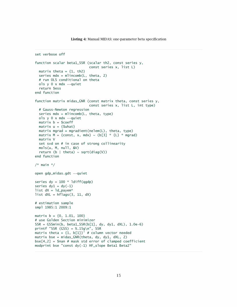
Listing 4: Manual MIDAS: one-parameter beta specification

set verbose off

function scalar beta1_SSR (scalar th2, const series y,const series x, list L)

matrix theta = {1, th2}series mdx = mlincomb(L, theta, 2)# run OLS conditional on thetaols y 0 x mdx --quietreturn $ess

end function

function matrix midas_GNR (const matrix theta, const series y,const series x, list L, int type)

# Gauss-Newton regressionseries mdx = mlincomb(L, theta, type)ols y 0 x mdx --quietmatrix b = $coeffmatrix u = {$uhat}matrix mgrad = mgradient(nelem(L), theta, type)matrix M = {const, x, mdx} ~ (b[3] * {L} * mgrad)matrix Vset svd on # in case of strong collinearitymols(u, M, null, &V)return (b | theta) ~ sqrt(diag(V))

end function

/* main */

open gdp_midas.gdt --quiet

series dy = 100 * ldiff(qgdp)series dy1 = dy(-1)list dX = ld_payem*list dXL = hflags(3, 11, dX)

# estimation samplesmpl 1985:1 2009:1

matrix b = {0, 1.01, 100}# use Golden Section minimizerSSR = GSSmin(b, beta1_SSR(b[1], dy, dy1, dXL), 1.0e-6)printf "SSR (GSS) = %.15g\n", SSRmatrix theta = {1, b[1]}’ # column vector neededmatrix bse = midas_GNR(theta, dy, dy1, dXL, 2)bse[4,2] = $nan # mask std error of clamped coefficientmodprint bse "const dy(-1) HF_slope Beta1 Beta2"

15

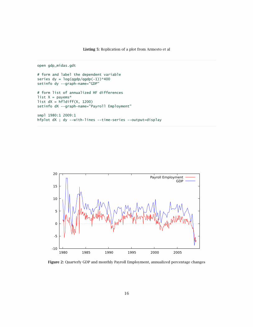
Listing 5: Replication of a plot from Armesto et al

open gdp_midas.gdt

# form and label the dependent variableseries dy = log(qgdp/qgdp(-1))*400setinfo dy --graph-name="GDP"

# form list of annualized HF differenceslist X = payems*list dX = hfldiff(X, 1200)setinfo dX --graph-name="Payroll Employment"

smpl 1980:1 2009:1hfplot dX ; dy --with-lines --time-series --output=display

-10

-5

0

5

10

15

20

1980 1985 1990 1995 2000 2005

Payroll EmploymentGDP

Figure 2: Quarterly GDP and monthly Payroll Employment, annualized percentage changes

16

Another sort of plot which may be useful shows the “gross” coefficients on the lags of thehigh-frequency series in a MIDAS regression—that is, the normalized weights multiplied bythe HF_slope coefficient. After estimation of a MIDAS model in the gretl GUI this is availablevia the item MIDAS coefficients under the Graphs menu in the model window. It is also easilygenerated via script, since the $model bundle that becomes available following the midasregcommand contains a matrix, midas_coeffs, holding these coefficients. So the following issufficient to display the plot:

matrix m = $model.midas_coeffsgnuplot --matrix=m --with-lp --fit=none --output=display \{ set title "MIDAS coefficients"; set ylabel ’’; }

Caveat: this feature is at present available only for models with a single MIDAS specification.

References

Armesto, M. T., K. Engemann and M. Owyang (2010) ‘Forecasting with mixed frequencies’, Fed-eral Reserve Bank of St. Louis Review 92(6): 521–536. URL http://research.stlouisfed.org/publications/review/10/11/Armesto.pdf.

Davidson, R. and J. G. MacKinnon (2004) Econometric Theory and Methods, New York: OxfordUniversity Press.

Ghysels, E. (2015) ‘MIDAS Matlab Toolbox’. University of North Carolina, Chapel Hill. URLhttp://www.unc.edu/~eghysels/papers/MIDAS_Usersguide_V1.0.pdf.

Ghysels, E. and H. Qian (2016) ‘Estimating MIDAS regressions via OLS with polynomial pa-rameter profiling’. University of North Carolina, Chapel Hill, and MathWorks. URL http://dx.doi.org/10.2139/ssrn.2837798.

Ghysels, E., P. Santa-Clara and R. Valkanov (2004) ‘The MIDAS touch: Mixed data samplingregression models’. Série Scientifique, CIRANO, Montréal. URL http://www.cirano.qc.ca/files/publications/2004s-20.pdf.

17

Appendix A: alternative MIDAS data methods

Importation via a column vector

Listing 6 illustrates how one can construct via hansl a “midas list” from a matrix (column vec-tor) holding data of a higher frequency than the given dataset. In practice one would probablyread high frequency data from file using the mread function, but here we just construct anartificial sequential vector.

Note the check in the high_freq_list function: we determine the current sample size, T, andinsist that the input matrix is suitably dimensioned, with a single column of length equal to Ttimes the compaction factor (here 3, for monthly to quarterly).

Listing 6: Create a midas list from a matrix

function list high_freq_list (const matrix x, int compfac, string vname)list ret = nullscalar T = $nobsif rows(x) != compfac*T || cols(x) != 1

funcerr "Invalid x matrix"endifmatrix m = mreverse(mshape(x, compfac, T))’loop i=1..compfac --quietscalar k = compfac + 1 - iret += genseries(sprintf("%s%d", vname, k), m[,i])

endloopsetinfo ret --midasreturn ret

end function

# construct a little "quarterly" datasetnulldata 12setobs 4 1980:1

# generate "monthly" data, 1,2,...,36matrix x = seq(1,3*$nobs)’print x# turn into midas listlist H = high_freq_list(x, 3, "test_m")print H --byobs

The final command in the script should produce

test_m3 test_m2 test_m1

1980:1 3 2 11980:2 6 5 41980:3 9 8 7...

This functionality is available in the built-in function hflist, which has the same signature asthe hansl prototype above.

18

Importation via join

Listing 7 illustrates how join can be used to pull higher-frequency data (in this example,quarterly) into a lower frequency (annual) dataset. The example is artificial, in that we have noactual annual data in view; consider it just as “proof of concept.”

We begin by opening the Area-Wide Model (AWM) quarterly dataset and writing three series to aCSV file: the year, the quarter, and the associated value of STN (short-term interest rate).

We then establish an annual dataset with the same temporal span as the AWM data, and usejoin to create four series from the CSV file, Eurorate_q4 to Eurorate_q1, matching rowsvia join’s tkey apparatus and filtering on the respective quarters. Partial output is shownbeneath the script.

At this point we’d be ready to append an actual annual series that’s of interest as a depen-dent variable, and estimate a model in which the quarterly interest-rate series figure as high-frequency independent variables.

Listing 7: Create a MIDAS dataset via join

open AWM --quietseries yr = $obsmajorseries qtr = $obsminor# STN = short-term interest ratestore @dotdir/tmp.csv yr qtr STN

# 116 quarters = 29 annual observationsnulldata 29# Annual data starting in 1970setobs 1 1970list ER = nullloop for (q=4; q>0; q--) --quietvname = sprintf("Eurorate_q%d", q)flt = sprintf("qtr==%d", q)join "@dotdir/tmp.csv" @vname --data=STN --tkey=",%YQ%q" --filter="@flt"ER += @vname

endloopsetinfo ER --midasprint ER -o

Eurorate_q4 Eurorate_q3 Eurorate_q2 Eurorate_q1

1970 7.1892 7.5600 7.8705 7.90321971 5.9811 6.2442 5.8679 6.27731972 6.3387 4.6302 4.6883 4.93611973 10.9720 9.9925 8.1424 6.75411974 10.6747 11.3925 11.0187 11.1175...

19

Appendix B: daily data

Daily data (commonly financial-market data) are often used in practical applications of theMIDAS methodology. It’s therefore important that gretl support use of such data, but thereare special issues arising from the fact that the number of days in a month, quarter or year isnot a constant. Here we describe the state of things as of September 19, 2017.

It seems to us that it’s necessary to stipulate a fixed, conventional number of days per lower-frequency period (that is, in practice, per month or quarter, since for the moment we’re ignor-ing the week as a basic temporal unit and we’re not yet attempting to support the combinationof annual and daily data). But matters are further complicated by the fact that daily data comein (at least) three sorts: 5 days per week (as in financial-market data), 6-day (some commercialdata which skip Sunday) and 7-day.

That said, we currently support—via compact=spread, as described in section 1—the follow-ing conversions:

• Daily to monthly: If the daily data are 5-days per week, we impose 22 days per month.This is the median, and also the mode, of weekdays per month, although some monthshave as few as 20 weekdays and some have 23. If the daily data are 6-day we impose 26days per month, and in the 7-day case, 30 days per month.

• Daily to quarterly: In this case the stipulated days per quarter are simply 3 times thedays-per-month values specified above.

So, given a daily dataset, you can say

dataset compact 12 spread

to convert MIDAS-wise to monthly (or substitute 4 for 12 for a quarterly target). And this issupposed to work whether the number of days per week is 5, 6 or 7.

That leaves the question of how we handle cases where the actual number of days in thecalendar month or quarter falls short of, or exceeds, the stipulated number. We’ll talk thisthrough with reference to the conversion of 5-day daily data to monthly; all other cases areessentially the same, mutatis mutandis.8

We start at “day 1,” namely the first relevant daily date within the calendar period (so thefirst weekday, with 5-day data). From that point on we fill up to 22 slots with relevant dailyobservations (including, not skipping, NAs due to holidays or whatever). If at the end we havedaily observations left over, we ignore them. If we’re short we fill the empty slots with thearithmetic mean of the valid, used observations;9 and we fill in any missing values in the sameway.

This means that lags 1 to 22 of 5-day daily data in a monthly dataset are always observa-tions from days within the prior month (or in some cases “padding” that substitutes for suchobservations); lag 23 takes you back to the most recent day in the month before that.

Clearly, we could get a good deal fancier in our handling of daily data: for example, lettingthe user determine the number of days per month or quarter, and/or offering more elaboratemeans of filling in missing and non-existent daily values. It’s not clear that this would beworthwhile, but it’s open to discussion.

A little daily-to-monthly example is shown in Listing 8 and Figure 3. The example exercises thehfplot command (see section 7).

8Or should be! We’re not ready to guarantee that just yet.9This is the procedure followed in some example programs in the MIDAS Matlab Toolbox.

20

Listing 8: Monthly plus daily data

# open a daily datasetopen djclose.gdt

# spread the data to monthlydataset compact 12 spreadlist DJ = djc*

# import an actual monthly seriesopen fedstl.bindata indpro

# high-frequency plothfplot DJ ; indpro --with-lines --output=daily.pdf \{set key top left;}

500

1000

1500

2000

2500

3000

1980 1982 1984 1986 1988 1990 48

50

52

54

56

58

60

62

64

66djclose (left)

indpro (right)

Figure 3: Monthly industrial production and daily Dow Jones close

21

Appendix C: parameterization functions

Here we give some more detail of the MIDAS parameterizations supported by gretl.

In general the normalized coefficient or weight i (i = 1, . . . , p) is given by

wi =f(i, θ)∑pi=1 f(i, θ)

(1)

such that the coefficients sum to unity.

In the normalized exponential Almon case with k parameters the function f(·) is

f(i, θ) = exp

k∑j=1

θjij (2)

So in the usual two-parameter case we have

wi =exp

(θ1i+ θ2i2

)∑pi=1 exp (θ1i+ θ2i2)

and equal weighting is obtained when θ1 = θ2 = 0.

In the standard, two-parameter normalized beta case we have

f(i, θ) = (i−/p−)θ1−1 · (1− i−/p−)θ2−1 (3)

where p− = p − 1, and i− = i − 1 except at the end-points, i = 1 and i = p, where we addand subtract, respectively, machine epsilon to avoid numerical problems. This formulationconstrains the coefficient on the last lag to be zero—provided that the weights are decliningat higher lags, a condition that is ensured if θ2 is greater than θ1 by a sufficient margin. Thespecial case of θ1 = θ2 = 1 yields equal weights at all lags. A third parameter can be usedto allow a non-zero final weight, even in the case of declining weights. Let wi denote thenormalized weight obtained by using (3) in (1). Then the modified variant with additionalparameter θ3 can be written as

w(3)i = wi + θ3

1+ pθ3

That is, we add θ3 to each weight then renormalize so that the w(3)i values again sum to unity.

In Eric Ghysels’ Matlab code the two beta variants are labeled “normalized beta density with azero last lag” and “normalized beta density with a non-zero last lag” respectively. Note thatwhile the two basic beta parameters must be positive, the third additive parameter may bepositive, negative or zero.

In the case of the plain Almon polynomial, coefficient i is given by

wi =k∑j=1

θjij−1

Note that no normalization is applied in this case, so no additional coefficient should be placedbefore the MIDAS lags term in the context of a regression.

22

Analytical gradients

Here we set out the expressions for the analytical gradients produced by the mgradient func-tion, and also used internally by the midasreg command. In these expressions f(i, θ) shouldbe understood as referring back to the specific forms noted above for the exponential Almonand beta distributions.

For the normalized exponential Almon case, the gradient is

dwidθj

= f(i, θ)ij∑i f(i, θ)

− f(i, θ)[∑i f(i, θ)

]2 ∑i

[f(i, θ)ij

]

= wi

ij − ∑i[f(i, θ)ij

]∑i f(i, θ)

For the two-parameter normalized beta case it is

dwidθ1

= f(i, θ) log(i−/p−)∑i f(i, θ)

− f(i, θ)[∑i f(i, θ)

]2 ∑i

[f(i, θ) log(i−/p−)

]

= wi(

log(i−/p−)−∑i[f(i, θ) log(i−/p−)

]∑i f(i, θ)

)

dwidθ2

= f(i, θ) log(1− i−/p−)∑i f(i, θ)

− f(i, θ)[∑i f(i, θ)

]2 ∑i

[f(i, θ) log(1− i−/p−)

]

= wi(

log(1− i−/p−)−∑i[f(i, θ) log(1− i−/p−)

]∑i f(i, θ)

)

And for the three-parameter beta, we have

dw(3)idθ1

= 11+ pθ3

dwidθ1

dw(3)idθ2

= 11+ pθ3

dwidθ2

dw(3)idθ3

= 11+ pθ3

− p(wi + θ3)(1+ pθ3)2

For the (non-normalized) Almon polynomial the gradient is simply

dwidθj

= ij−1

23