Gretl TutorialGretl Tutorial I: The Basics

Gretl Tutorial II: OLS Regression

Gretl Tutorial III: Diagnostics – “He’s dead, Jim”

Gretl Tutorial IV: Seasonal Dummies

Gretl Tutorial I: The Basics

Following on from this post, I'm going to use Malaysian export/import data (as in my trade posts e.g. here) to illustrate how to use Gretl to create a simple trade forecast model, essentially recreating the two forecast models I've been using previously.

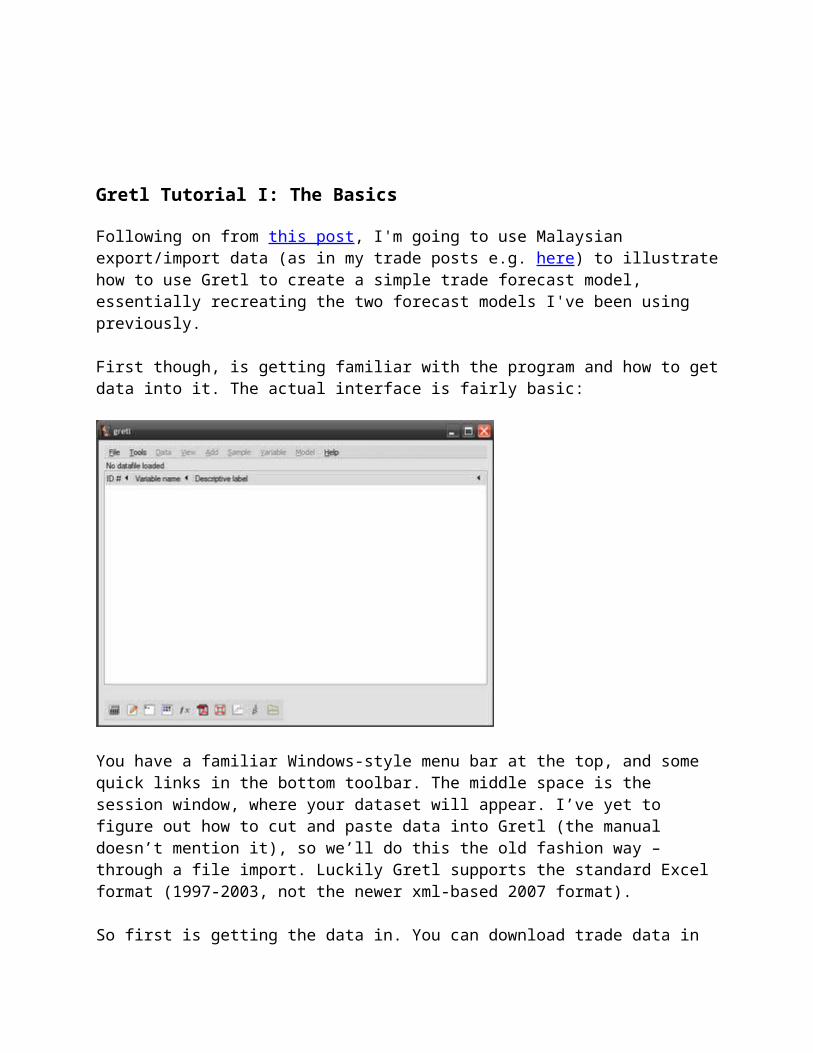
First though, is getting familiar with the program and how to get data into it. The actual interface is fairly basic:

You have a familiar Windows-style menu bar at the top, and some quick links in the bottom toolbar. The middle space is the session window, where your dataset will appear. I’ve yet to figure out how to cut and paste data into Gretl (the manual doesn’t mention it), so we’ll do this the old fashion way – through a file import. Luckily Gretl supports the standard Excel format (1997-2003, not the newer xml-based 2007 format).

So first is getting the data in. You can download trade data in Excel format from Bank Negara’s Monthly Statistical Bulletin (the June 2009 edition):

…which should give you this:

Unfortunately, the data is not in flat file format but more a representation of the actual printed copy, so some manipulation is in order here. First is expanding the whole spreadsheet to fully expose the data-points. Select the entire spreadsheet by left-clicking on the top-leftmost cell header (left of the “A” column header), then right click on any of the row headers and select “Unhide”:

Scrolling down, you should now see the full spreadsheet, with annual data from 1975, quarterly data from 1996, and monthly data from 1996. Select the monthly data for exports and imports from 1996 to 2009:

…and copy it to a new Excel book, then type “Exports” for the first data column and “Imports” for the second data column. You should get this:

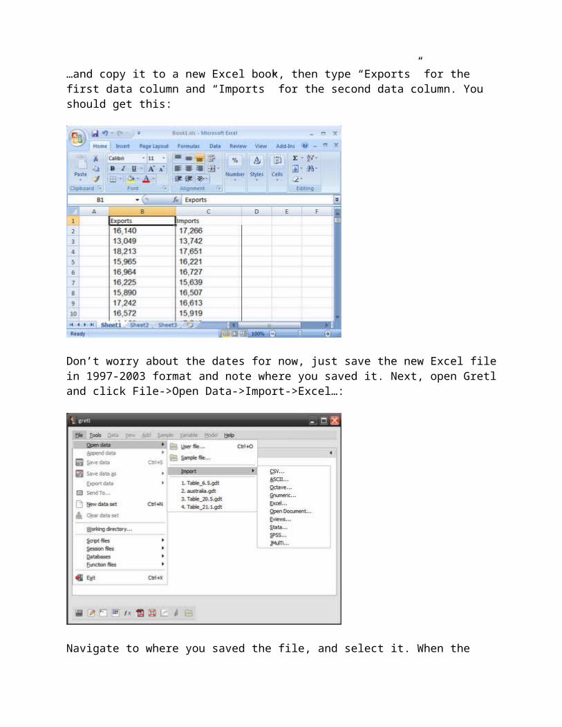
Don’t worry about the dates for now, just save the new Excel file in 1997-2003 format and note where you saved it. Next, open Gretl and click File->Open Data->Import->Excel…:

Navigate to where you saved the file, and select it. When the file opens, select "Ok" then “Yes”:

…click “Time Series”, then “Forward”:

…click “Monthly”, then “Forward”:

Since our dataset begins in January 1996, change the value to “1996:01”, then “Forward”:

…Click “Apply”:

…and you should now have an “Export” variable and “Import” variable in your session window. To confirm, you can right click on any of the variables and select “Display values”, which should give you something like this:

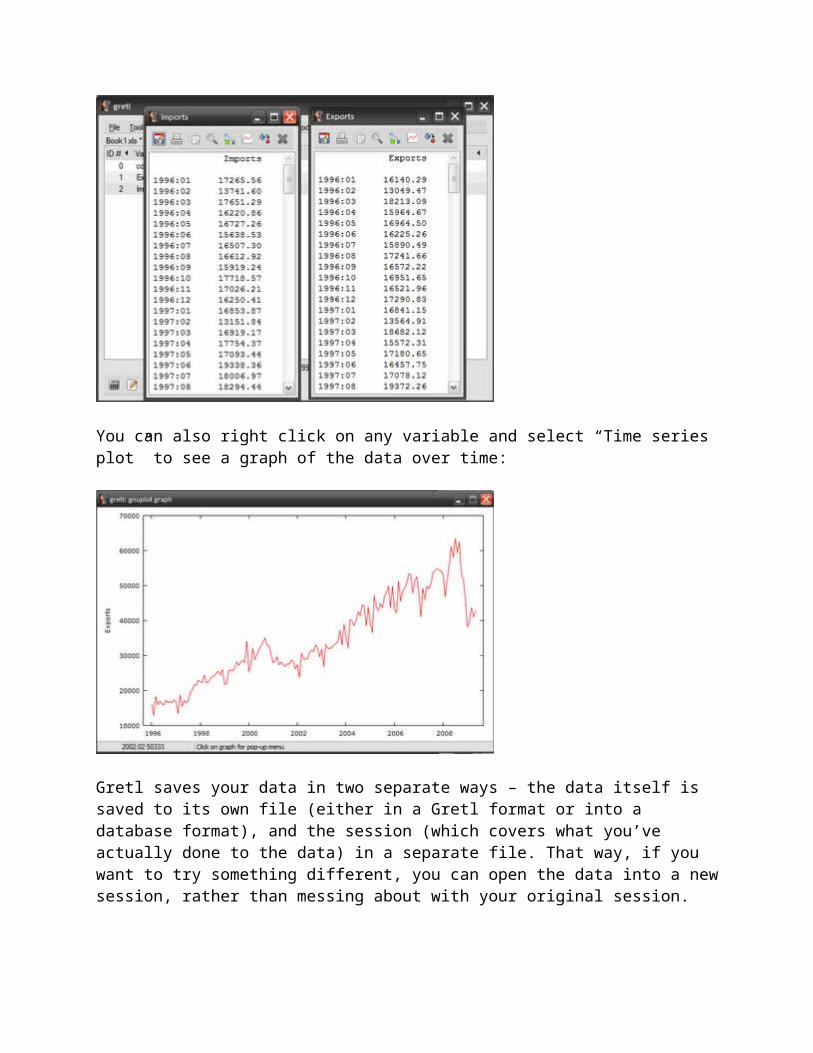
You can also right click on any variable and select “Time series plot” to see a graph of the data over time:

Gretl saves your data in two separate ways – the data itself is saved to its own file (either in a Gretl format or into a database format), and the session (which covers what you’ve actually done to the data) in a separate file. That way, if you want to try something different, you can open the data into a new session, rather than messing about with your original session.

The next tutorial will cover regression estimation based on the trade data you’ve loaded into the program.

Gretl Tutorial II: OLS Regression

Gretl Tutorial I

Now that we have a dataset to play with, what can we do with it?

I based my simple trade models on the assumption that Malaysian imports and exports are cointegrated i.e. that there is a long term relationship between the two variables.

Intuitively, since 70%+ of imports are composed of intermediate goods, which are goods used as inputs into making other goods (including exports), we would expect a statistically significant relationship between exports and imports. For instance, exporters would have certain expectations of demand (advance orders) and order inputs based on that demand. After processing, the finished goods would then be exported.

In such a case, imports of inputs would lead exports by a time factor, depending on the length of time engaged in processing. This is something we can actually test, but I’ll leave that for later and just assume a lag of 1 month. Since imports are based on expected future export demand, we can then use imports to actually forecast exports.

There are some problems with making such a simplistic assumption of course (e.g. how do we account for exports with no foreign inputs), but since this is a demonstration of regression analysis and not an econometric examination of the structure of Malaysian trade, we’ll ignore it for now. In any case, for forecasting purposes, structure (economically accurate modeling) is less important than a usable and timely forecast.

If you’ve gone through the previous post, you’ll have export and import data loaded into Gretl and ready to go. The first step is to transform the data to natural logs. Select both variables (Ctrl-click), then go to the menubar and click Add->Logs of selected variables:

You’ll now have two additional variables called l_imports and l_exports:

The reasons we transform into natural log form is twofold: most economic time series are characteristically exponential with respect to time, and a log transformation changes the vertical scale to linear. Log transformations also make elasticity calculations easier, as the estimated coefficients are approximate to percentage changes in the variables.

To estimate the regression, click Model->Ordinary least squares…:

…which will give the model specification screen:

Select l_exports then click on the “Choose” button, which sets the log of exports as the dependent variable. Then select l_imports and click the “Add” button, which sets the log of imports as the explanatory variable. At this stage, you should note that the “lags…” button turns from greyed out to normal. Click on this, which brings up the lag screen:

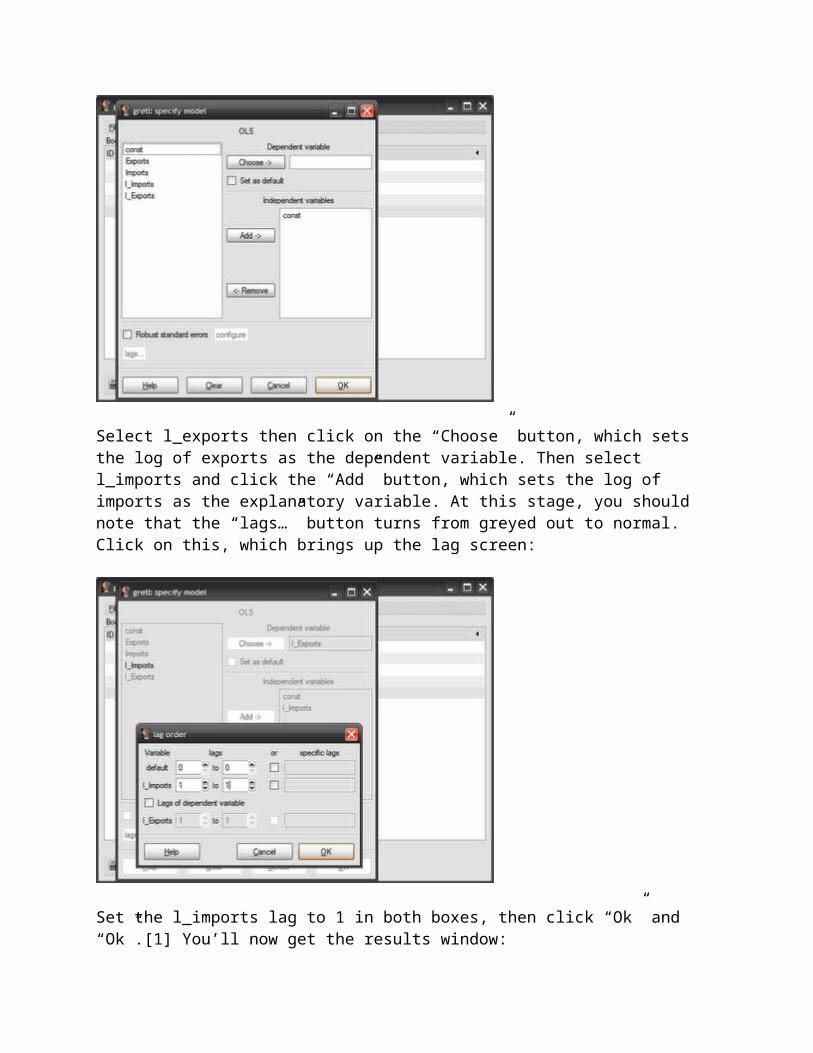
Set the l_imports lag to 1 in both boxes, then click “Ok” and “Ok”.[1] You’ll now get the results window:

Don’t worry if the results window looks complicated, there’s only a few numbers that you really have to deal with...for now. First are the results of the estimation itself:

(l_exports)=-0.551950+1.07273(l_imports(-1))

The interpretation here is that a 1% rise in last month's imports causes a 1.07% rise in this month's exports. To have a look at your work, click Graphs->Fitted, actual plot->Against time, in the results window:

You should see this:

The red line displays actual values of l_exports, while the blue line represents the values from your estimated equation. Note that before 2000 the forecast errors are fairly large compared to after 2000, both under- and over-estimating exports. On the whole however, the results of the equation looks good, and seems to be a fairly accurate forecast model for exports.

Now, that wasn't so hard was it?

But we still have to be sure that this is a statistically significant relationship. Ordinarily, this involves a hypothesis test of the coefficients (null hypothesis=0), which involves using the standard errors to calculate a T-ratio, which is then evaluated against the critical values in a Student's T table.[2]

Since busy people can’t be bothered with stuff like that, Gretl very nicely lets you skip all those steps – all you have to pay attention to is the p-value. I could give a technical explanation for what it is, but all you have to know is that [1-(p-value) x 100] gives the confidence level. So if the p-value is 0.05, then you are 95% confident that the estimated coefficient is statistically significantly different from zero (statistically significant for short).

You can skip even this step, and just look at the stars Gretl appends on the right side of the p-value. One * means a 90% confidence level, ** means a 95% confidence level, and *** means a 99% confidence level. Just like hotels and restaurants, the more stars the better.

In the case of this estimation, we are 93.5% confident that the constant is statistically significant and 99.999% confident that the coefficient for l_imports is statistically significant.

You now have what appears to be a decent model for estimating future exports, at least for a 1-month ahead forecast. But since forecasting can’t be obviously so simple, we’ll look at some of the necessary tests to do to confirm we have a econometrically solid model to rely on.

[1] You can skip this step by directly specifying the lagged data series in the session screen. Select the variable you want then click Add->Lags of selected variables, then select the number of lags you want. Then in the model screen, select the lagged variable as the explanatory variable, rather than the original explanatory variable. Whether you take this step or the one I explained above, a lagged data series will be added to your dataset.

[2] You can do this manually within Gretl if you’re masochistic. The critical values can be accessed in the session screen, by clicking Tools->Statistical Tables, then selecting “t” from the tabs. Put value 160 in the “df” (“degrees of freedom”) box, and 0.025 in the “right-tail probability” box which corresponds to a two-tail 95% confidence level test. You should get a critical value of 1.9749. Since the constant has a t-ratio of -1.856, it is not statistically significant, but the coefficient for l_imports has a t-ratio of 36.36 which means it is at the 95% confidence level. You can vary the value for the “right-tail probability” box to obtain the critical values for other confidence levels.

Gretl Tutorial III: Diagnostics – “He’s dead, Jim”

Gretl Tutorial I

Gretl Tutorial II

Now that we have a decent regression that seemingly outlines a plausible relationship between exports and lagged imports, we have to test from a statistical perspective whether we can make inferences from the resulting equation. That will determine whether we can actually make statistically reliable forecasts. So what are the potential problems we can encounter?

Papering over an academic discussion of the properties of estimators, from a simplistic perspective what we are trying to achieve is a model where coefficient estimates are unbiased, efficient, linear and consistent. This is actually best achieved not by looking at the estimators themselves but by looking at the residuals, which is the difference between the actual data and the estimated relationship. You can get view the residuals in Gretl by looking at the results screen, selecting Graphs->Residual plot->Against time:

A cursory examination of the residuals is revealing. As I noted earlier, there’s a discontinuity between our results and the actual data for the period before 2000. Also there’s a marked seasonal pattern in the residuals, which means seasonality is a factor as well. But I’m leaving that for the next post, which will deal with dummy variables. For now, I want to look at some of the standard diagnostic tests that are typically used to make sure our model is a valid one.

The two main problems with times series deal with the requirement that residuals must be independent and normally distributed:

1. Serial correlation – which means residuals are not independent over time, and are in fact correlated;

2. Heteroscedasticity – which means variance (and standard errors) are not constant, and thus residuals are not normally distributed.

There are a number of standard statistical tests that can be performed to find out whether either of these two conditions hold; if they do, then we have to rethink our model.

The most common method to test for serial correlation is one you don’t have to perform; both Gretl (and EViews) report the Durbin-Watson statistic as part of the estimation results. In the Gretl results screen, it is the last number reported in the right column, with a value of 1.807829. The actual test statistic requires some calculation but essentially a value of 2 means no serial correlation, while a value of 4 or 0 mean perfect positive or negative correlation. As a short cut, in the results screen you can select Tests->Durbin-Watson p-value which gives a p-value of 0.097161, indicating that at the 95% confidence level you cannot reject the null hypothesis of no serial correlation:

Unfortunately the DW stat has a weakness in that it is only a valid test for serial correlation over 1 lag. For multiple lags, you need to use a different test. The Breusch-Godfrey test allows for this and can be reached at Tests->Autocorrelation (I’m using 12 lags here):

As you can see, while the BG test echoes the DW stat for the first lag, there is serial correlation at lags 2, 3, 5, 10, 11, and 12 (check the stars). All the test statistics (at the bottom of the test results page) show very small p-values, indicating a rejection of the null hypothesis of no serial correlation. Note that any tests you do are automatically added to the results page, below the estimation results – a nice touch.

To test for heteroscedasticity, select Tests->heteroskedasticity (sic)->White’s test:

The p-value is 0.000003, which means you have to reject the null hypothesis that there is no heteroscedasticity.

As an additional test, you can directly test whether the residuals are normally distributed (select Tests-> Normality of residual):

The p-value of 0.06723 means that it's a close run thing - you would accept the null hypothesis of normality at the 95% confidence level, but reject it at the 90% confidence level.

Lastly, I almost always test for ARCH (select Tests->ARCH):

Which suggests that ARCH is present as well. ARCH is a special form of heteroscedasticity – it’s an acronym that means auto-regressive conditional heteroscedasticity, and is especially common in financial markets. It’s also a rather fancy way of saying that volatility clumps together, as illustrated by this chart of daily log returns on the KLCI:

Going back to our trade model, we have some very obvious problems. With both heteroscedasticity and serial correlation present, I’d be very wary of relying on the model as it stands. To solve this, we need to relook the model specification – the pattern of residuals provides the main clue. We have to deal with seasonality, and we have to deal with a potential change in the relationship between exports and imports post-2000.

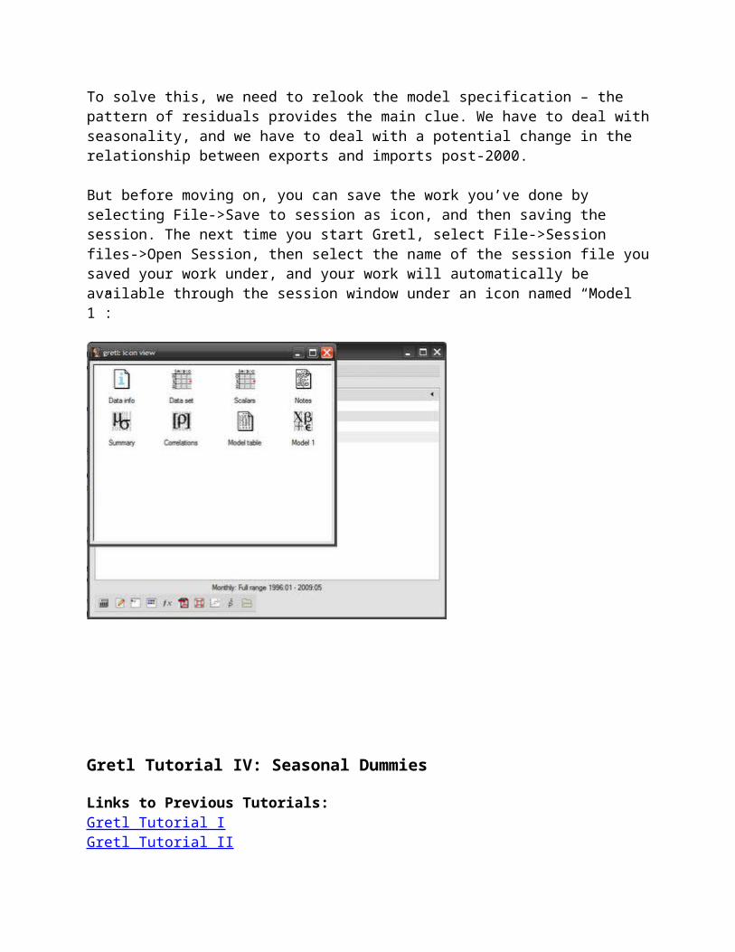
But before moving on, you can save the work you’ve done by selecting File->Save to session as

icon, and then saving the session. The next time you start Gretl, select File->Session files->Open Session, then select the name of the session file you saved your work under, and your work will automatically be available through the session window under an icon named “Model 1”:

Gretl Tutorial IV: Seasonal Dummies

Links to Previous Tutorials:Gretl Tutorial IGretl Tutorial IIGretl Tutorial III

No, this isn’t about intelligence-challenged seasonal heretics. In my last few posts, I’ve pointed out the big difference in the picture presented by the raw economic numbers and that shown after seasonal adjustment – which neatly leads me to the purpose of the tutorial today. In my last post on using Gretl, the basic export forecast model I created showed some problems in the diagnostics, with both heteroscedasticity (time-varying variance) and serial correlation (non-independent error terms) present in the model. I identified two potential areas in the model specification that may require looking into: seasonal variation and a structural break. I’ll deal with modeling the seasonal variation first and structural breaks later.

First some concepts: to model seasonality as well as structural breaks, we use what are called dummy variables which take the value of 1 or 0. For instance, a January dummy would have the

value of 1 for every January, and 0 for every other date. A structural break would have a value of 1 for every date before or after the date you think there is a break in the model, and 0 in every other date. Intuitively, the modeling procedure for seasonal dummies is that you are assuming that the trend is intact for the overall series, but that there are different intercepts for each month. For example, in the simple regression model:

Y = a + bX

we are assuming that there is a different value of a for every month. Structural breaks are harder, because you have the potential for a change in both the intercept as well as the slope, in other words both a and b could be different before and after the break. I’ll cover this in the next tutorial.

The actual procedure in Gretl is ridiculously easy. Load up the saved session from the past tutorials I covered (see top of this post), then select Add->Periodic dummies. Gretl automatically defines the variables for you in the session window:

Just to be sure, double-click on the dm1 dummy, and verify that the values for January (denoted as :01) are all 1, and the values for other months are 0:

To create a new model using these new variables, open up the model specification screen by selecting from the session window Model -> Ordinary least squares:

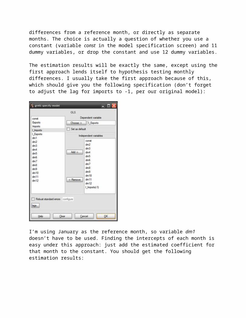
You now a choice to make – you can model seasonal variation as differences from a reference month, or directly as separate months. The choice is actually a question of whether you use a constant (variable const in the model specification screen) and 11 dummy variables, or drop the constant and use 12 dummy variables.

The estimation results will be exactly the same, except using the first approach lends itself to hypothesis testing monthly differences. I usually take the first approach because of this, which should give you the following specification (don’t forget to adjust the lag for imports to -1, per our original model):

I’m using January as the reference month, so variable dm1 doesn’t have to be used. Finding the intercepts of each month is easy under this approach: just add the estimated coefficient for that month to the constant. You should get the following estimation results:

Looking at the p-values and stars on the right hand side (see this post for definitions), both the constant and the log of imports are statistically significant at the 99% level. Compare this with our original model:

The intercept (the const variable) has fallen, while the slope (the coefficient for l_imports_1) has steepened. The R-squared number (the third row in the column of numbers below the results) measures how good a fit the model is with the data, with a value of 1 meaning a perfect match. R-squared in model2 has increased to 0.93 from 0.89 in model 1 – so our new model is a closer fit to the data, though not much more. Looking at the residuals (differences between the model and the actual data), our model 2 has gotten rid of some of the sharper spikes in the data, and the

graph more closely approximates random noise (model 1 in red, model2 in blue):

Running through the diagnostics (see this post), it looks like I still have serial correlation and heteroscedasticity, but the distribution of the residuals is more “normal”:

So the problems haven’t been solved by modeling seasonal variation, but we’ll leave that here to move on to seasonal adjustment.

The whole rigmarole of going through the above process is to illustrate some key concepts of seasonal adjustment mechanisms. By estimating the intercepts of each month, you can now construct a seasonal “index” – how different each month is to each other. A simple way to do this is to calculate each monthly intercept as a percentage of the average of all of them together. The resulting percentages can then be applied back to the data – you multiply each monthly data point by the index percentage for that month. Voila! You’ve now seasonally adjusted your data.

In practice, geometric averaging is preferred, and there’s also some modeling of business cycles which don’t necessarily follow a seasonal pattern. And since Gretl is a software package, it has the ability to do the whole thing for you although it does require you to add a separate third-party package.

Go back to the Gretl homepage, and you’ll see some downloads available as optional extras. The one’s you want are X-12-ARIMA and TRAMO/SEATS, which are used respectively in the US and Europe. Download and install either (or both), then save and restart the Gretl program. In the session screen, select the Exports series in the window, then select from the menubar Variable->X-12-ARIMA analysis (I found this to be really buggy, so save your session before and after you get the results):

Click on the Save data: Seasonally adjusted series box and select Ok:

And you’ll get this nice graph:

But more importantly, you get a new variable called Expo_d11 which is the seasonally adjusted series for Exports. You can do the same thing for imports, and rerun the models or just compare the series to see how different they are. To do the latter, just select any two series (like the export series), right click and select Time series plot:

Choose your graph preference:

Which yields:

That’s it for today. Next up – breakdancing. Posted by hishamh at 10:45 AM Email This BlogThis! Share to Twitter Share to Facebook Share to Google Buzz Labels: exports, external trade, Gretl, imports, seasonal adjustment, seasonal effects Reactions: 

3 comments:

nickboafo said...

Hi,

I am new in this system here, and I was follwing the Gretl very closely. Now I am trying to use it for Cointegration and ECM. Any suggestion on how to go about them? I need help on these please.

Nick

January 20, 2011 6:46 PM

hishamh said...

Hi Nick,

The best I can do for you is to advise you to beg, borrow or steal this book. It's an almost step by step guide to cointegration - expensive and technical in parts, but worth every penny.

Second best thing I can do is the basic steps:

1. Test variables for stationarity (unit root tests - ADF and/or PP). Variables I(1) or higher should be treated as endogenous, I(0) as exogenous;2. Estimate an unrestricted VAR(x), where x is the number of lags (chosen or tested);2. Do cointegration testing based on VAR(x-1) - Gretl has the correct tests available;3. Based on the results, specify VECM(x-1) (restricted VAR) based on the number of cointegrating equations found;4. Normalise the error correction terms - i.e. rank the endogenous variables based on significance in the error correction terms;5. Test each variable for weak exogeneity (statistical significance). If any variables are not statistically significant than zero, the VECM should be re-estimated with these variables restricted to zero (both in error correction terms and in the cointegrating equations).6. Analysis

Also, depending on the nature of your data, you might need to test for structural breaks and insert dummy variables (treated as exogenous) in the VECM.

You might have to repeat all the steps depending on your data - I find it helps to have multiple proxies of the variables you're interested in, in case the final VECM doesn't make sense (potential omitted variable bias, wrong signs, non-significance when you expect significance or vice-versa).

Good Luck!