microscopic momentum balance equation (navier-stokes)fmorriso/cm310/lectures/2019... ·...

Fluids Lecture 5 Morrison CM3110 11/3/2019

1

© Faith A. Morrison, Michigan Tech U.

CM3110 Transport IPart I: Fluid Mechanics

Professor Faith Morrison

Department of Chemical EngineeringMichigan Technological University

1

Microscopic Momentum Balance Equation (Navier-Stokes)

Microscopic Balances


We have been doing a microscopic control volume balance; these are specific to whatever problem we are solving.

dx

dy

dz

We seek equations for microscopic mass, momentum (and energy) balances that are general.

•equations must not depend on the choice of the control volume,

•equations must capture the appropriate balance

2

Microscopic Momentum Balance Equation (Navier‐Stokes)


2

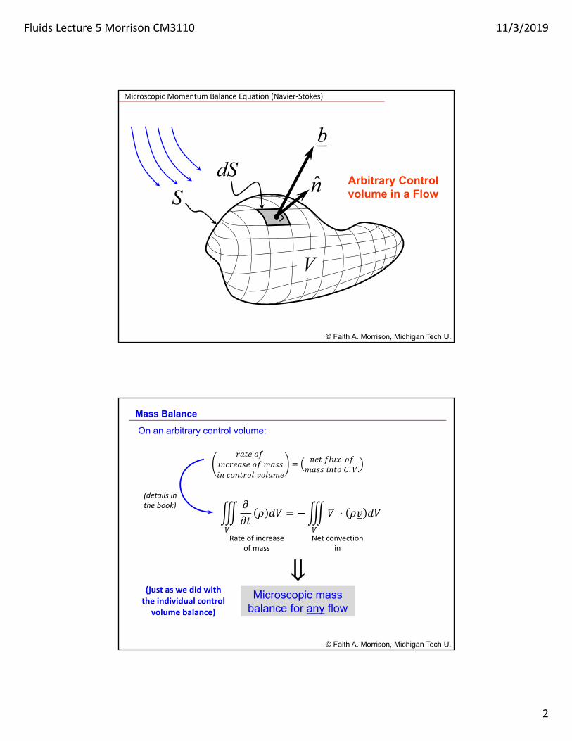
Arbitrary Control volume in a Flow


V

nS

b

dS``


Mass Balance


On an arbitrary control volume:

Microscopic mass balance for any flow

Rate of increase of mass

Net convection in

⇒

(just as we did with the individual control volume balance)

𝑟𝑎𝑡𝑒 𝑜𝑓 𝑖𝑛𝑐𝑟𝑒𝑎𝑠𝑒 𝑜𝑓 𝑚𝑎𝑠𝑠𝑖𝑛 𝑐𝑜𝑛𝑡𝑟𝑜𝑙 𝑣𝑜𝑙𝑢𝑚𝑒

𝑛𝑒𝑡 𝑓𝑙𝑢𝑥 𝑜𝑓𝑚𝑎𝑠𝑠 𝑖𝑛𝑡𝑜 𝐶.𝑉.

𝜕𝜕𝑡

𝜌 𝑑𝑉 𝛻 ⋅ 𝜌𝑣 𝑑𝑉

(details in the book)


3

Continuity Equation

V

ndSS

Microscopic mass balance written on an arbitrarily shaped control volume, V, enclosed by a surface, S

z

v

y

v

x

v

zv

yv

xv

tzyx

zyx

Gibbs notation:

© Faith A. Morrison, Michigan Tech U.5

Microscopic mass balance is a scalar equation.

𝜕𝜌𝜕𝑡

𝑣 ⋅ 𝛻𝜌 𝜌 𝛻 ⋅ 𝑣

Momentum Balance


On an arbitrary control volume:

Microscopic momentum balance

for any flow

Rate of increase of momentum

Net convection in

Force due to gravity

Viscous forces and pressure

forces ⇒

𝑟𝑎𝑡𝑒 𝑜𝑓 𝑖𝑛𝑐𝑟𝑒𝑎𝑠𝑒𝑜𝑓 𝑚𝑜𝑚𝑒𝑛𝑡𝑢𝑚

𝑖𝑛 𝐶.𝑉.

𝑛𝑒𝑡 𝑓𝑙𝑢𝑥 𝑜𝑓𝑚𝑜𝑚𝑒𝑛𝑡𝑢𝑚 𝑖𝑛𝑡𝑜 𝐶.𝑉.

𝑠𝑢𝑚 𝑜𝑓 𝑓𝑜𝑟𝑐𝑒𝑠𝑜𝑛 𝐶.𝑉.

(just as we did with the individual control volume balance)

(details in the book)

𝜕𝜕𝑡

𝜌𝑣 𝑑𝑉 𝛻 ⋅ 𝜌𝑣𝑣 𝑑𝑉 𝜌𝑔 𝑑𝑉 𝛻 ⋅ Π 𝑑𝑉


4

Equation of Motion

V

ndSS

Microscopic momentumbalance written on an arbitrarily shaped control volume, V, enclosed by a surface, S

Gibbs notation: general fluid

Gibbs notation:Newtonian fluid

Navier‐Stokes Equation


Microscopic momentum balance is a vector equation.

𝜌𝜕𝑣𝜕𝑡

𝑣 ⋅ 𝛻𝑣 𝛻𝑝 𝛻 ⋅ �� 𝜌𝑔


𝑣 ⋅ 𝛻𝑣 𝛻𝑝 𝜇𝛻 𝑣 𝜌𝑔


© Faith A. Morrison, Michigan

8

www.chem.mtu.edu/~fmorriso/cm310/Navier.pdf

Continuity Equation (And Non‐Newtonian Equation) on the

The one with “𝝉” is for non‐

Newtonian fluids

𝜕𝜌𝜕𝑡

𝑣 ⋅ 𝛻𝜌 𝜌 𝛻 ⋅ 𝑣


5


9


Navier‐Stokes (Newtonian Fluids Only) is on the :

There are no “𝝉”`s on this side


𝑣 ⋅ 𝛻𝑣 𝛻𝑝 𝜇𝛻 𝑣 𝜌𝑔

Problem‐Solving Procedure – solving for velocity and stress fields

1. sketch system

2. choose coordinate system

3. simplify the continuity equation (mass balance)

4. simplify the 3 components of the equation of motion (momentum balance) (note that for a Newtonian fluid, the equation of motion is the Navier‐Stokes equation)

5. solve the differential equations for velocity and pressure (if applicable)

6. apply boundary conditions

7. calculate any engineering values of interest (flow rate, average velocity, force on wall)


amended: when using the microscopic balances

�� 𝜇 𝛻𝑣 𝛻𝑣 )


6

x

EXAMPLE I: Flow of a Newtonian fluid down an inclined plane

Revisited

g

z

xz

fluid

xvz

air

cos

0

sin

g

g

g

g

g

g

z

y

x

singgx

cosggz


H

EXAMPLE I: Flow of a Newtonian fluid down an inclined plane

Revisited


(see hand notes)


7

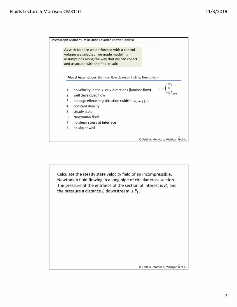
Model Assumptions: (laminar flow down an incline, Newtonian)

1. no velocity in the x‐ or y‐directions (laminar flow)

2. well developed flow

3. no edge effects in y‐direction (width)

4. constant density

5. steady state

6. Newtonian fluid

7. no shear stress at interface

8. no slip at wall


As with balance we performed with a control volume we selected, we made modelling assumptions along the way that we can collect and associate with the final result:

𝑣00𝑣

𝑣 𝑓 𝑦



Calculate the steady state velocity field of an incompressible, Newtonian fluid flowing in a long pipe of circular cross section. The pressure at the entrance of the section of interest is 𝑃 and the pressure a distance 𝐿 downstream is 𝑃 .


8

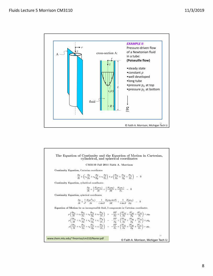
cross-section A:A

r z

r

z

L vz(r)

Rfluid

EXAMPLE II: Pressure‐driven flow of a Newtonian fluid in a tube: (Poiseuille flow)

•steady state•constant 𝜌•well developed•long tube•pressure 𝑝 at top•pressure 𝑝 at bottom

g



16



9


17


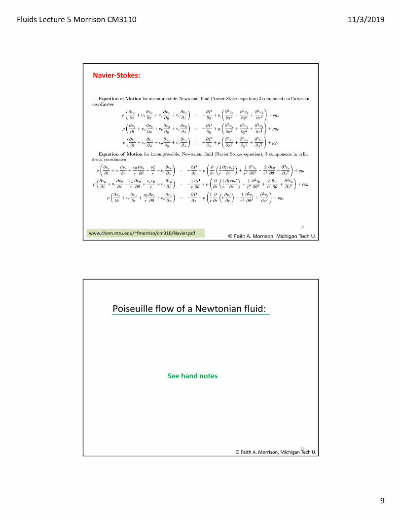
Navier‐Stokes:

Poiseuille flow of a Newtonian fluid:


See hand notes


10


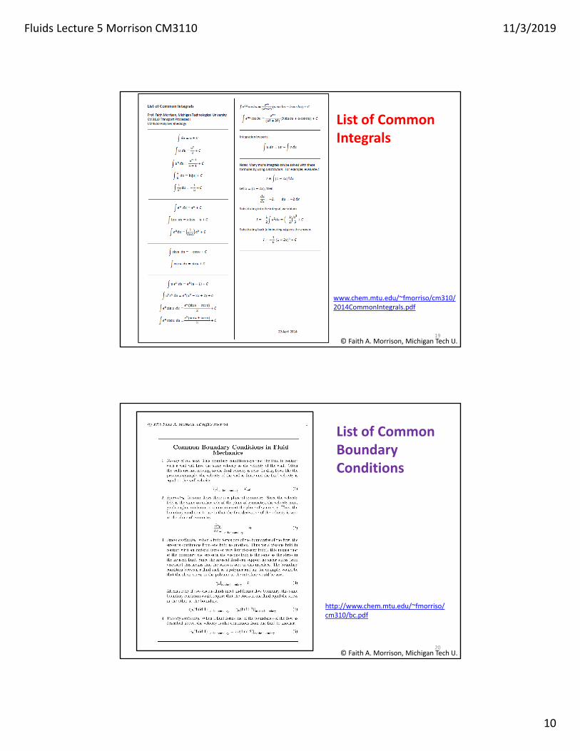
www.chem.mtu.edu/~fmorriso/cm310/2014CommonIntegrals.pdf

List of Common Integrals


http://www.chem.mtu.edu/~fmorriso/cm310/bc.pdf

List of Common Boundary Conditions


11

�� 𝑎𝑟𝑒𝑎



What is the force on the walls in this flow?cross-section A:

r

z

L vz(r)

Rfluid

forcearea

𝑎𝑟𝑒𝑎

Total wetted area

Inside surface of tube

? ?

y zstress on a y-surface in the z-direction

in the y-direction flux of z-momentum

2 //yz

kg m sforce kg m s

area area s area Momentum

Flux


9 stresses at a point in space

A surface whose unit

normal is in the y-direction

ye

f

22

yz

(See discussion of sign convention of stress; this is the tension-positive convention, �� )

𝑓 𝐴 ��


12



What is the shear stress in this flow?

�� 𝜇𝜕𝑣𝜕𝑟

Stress on an r surface in the z direction

cross-section A:

r

z

L vz(r)

Rfluid



See hand notes

Force on the walls:


13



𝑝 𝑧𝑝 𝑝𝐿

𝑧 𝑝

�� 𝑟𝜌𝑔𝐿 𝑝 𝑝

2𝐿𝑟

𝑣 𝑟𝑅 𝜌𝑔𝐿 𝑝 𝑝

4𝜇𝐿1

𝑟𝑅

average velocity

volumetric flow rate

z‐component of force on the wall


Engineering Quantities of Interest(tube flow)

26

Must work these out for each problem in the coordinate system in use; see inside back cover of book.

⟨𝑣 ⟩𝑣 𝑟𝑑𝑟𝑑𝜃

𝑟𝑑𝑟𝑑𝜃

𝑄⟩ 𝑣 𝑟𝑑𝑟𝑑𝜃 𝜋𝑅 ⟨𝑣 ⟩

𝐹 �� 𝑅𝑑𝜃𝑑𝑧


14

average velocity


𝑧‐component of force on the wall


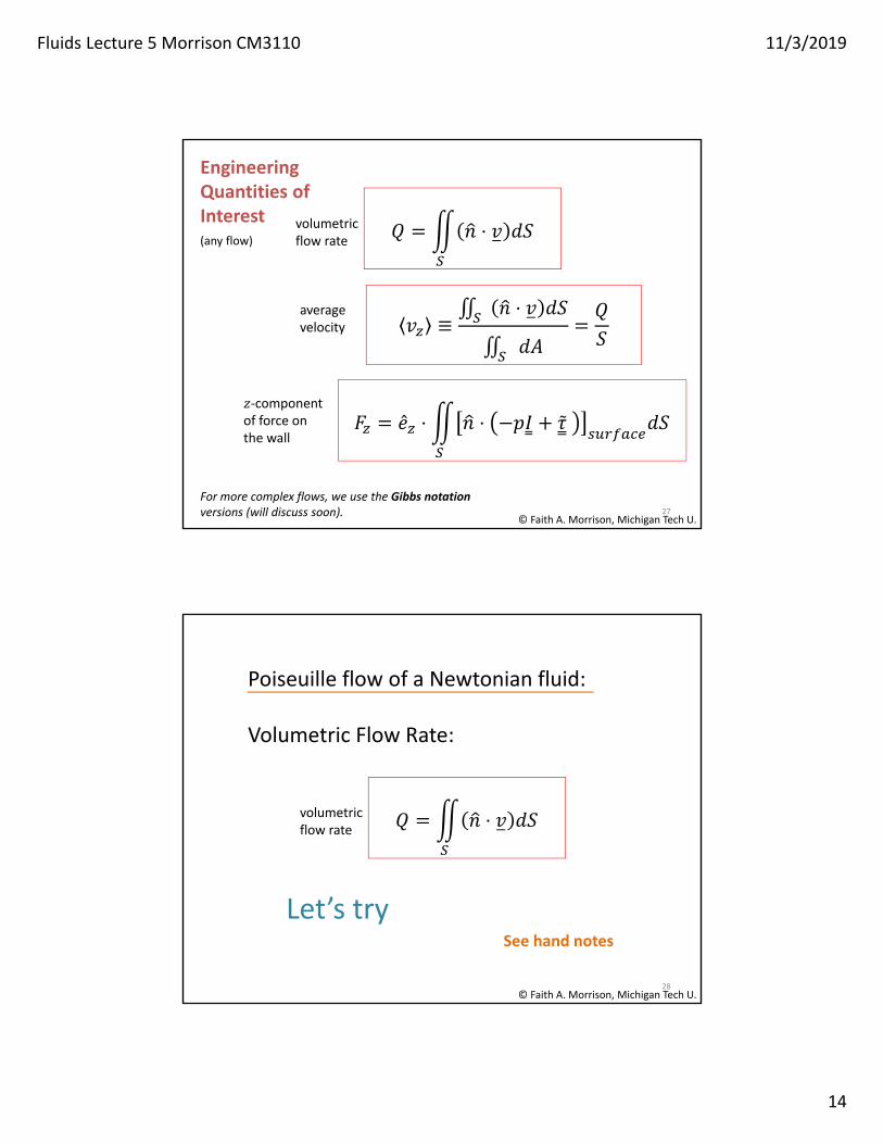
Engineering Quantities of Interest(any flow)

27

𝑣 ≡∬ 𝑛 ⋅ 𝑣 𝑑𝑆

∬ 𝑑𝐴

𝑄𝑆

𝑄 𝑛 ⋅ 𝑣 𝑑𝑆

𝐹 �� ⋅ 𝑛 ⋅ 𝑝�� 𝑑𝑆

For more complex flows, we use the Gibbs notation versions (will discuss soon).



See hand notes

Volumetric Flow Rate:


𝑄 𝑛 ⋅ 𝑣 𝑑𝑆

Let’s try


15



Hagen‐Poiseuille Equation**

29

𝑄𝜋𝑅 𝜌𝑔𝐿 𝑝 𝑝

8𝜇𝐿

𝑄 𝑣 𝑟 𝑟𝑑𝑟𝑑𝜃

𝑅 𝜌𝑔𝐿 𝑝 𝑝

4𝜇𝐿1

𝑟

𝑅𝑟𝑑𝑟𝑑𝜃

2

8

14

max,

2

2

0 0

22

2

0 0

z

Lo

RLo

R

zav

v

L

PPgLR

rdrdR

r

L

PPgLR

rdrdrvv




16


0

0.5

1

1.5

2

0 0.25 0.5 0.75 1

R

r

av

z

v

v

-1

-0.5

0

0 0.25 0.5 0.75 1L

z

Lpp

pp

0

0

31

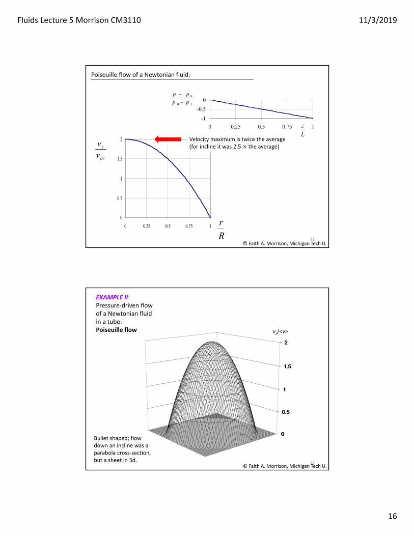
Velocity maximum is twice the average (for incline it was 2.5 the average)



vz/<v>

EXAMPLE II: Pressure‐driven flow of a Newtonian fluid in a tube: Poiseuille flow

32

Bullet shaped; flow down an incline was a parabola cross‐section, but a sheet in 3d.


17

A

xy

cross-section A:

z

xvz(x,y) H

Example III: Pressure-driven flow of a Newtonian fluid in a rectangular duct: Poiseuille flow


33

What is the steady state velocity profile for laminar flow of an incompressible Newtonian fluid flowing down a long duct of rectangular cross section? The duct height is 2𝐻 and the width is 2𝑊.The pressure at an upstream position is 𝑝 and a distance 𝐿 downstream the pressure is 𝑝 . What is the force on the walls?

See hand notes

(Example 7.11, p549)


Can this modeling method work for complex flows?

Answer: yes. (with some qualifiers)

microscopic momentum balance equation (navier-stokes)fmorriso/cm310/lectures/2019... ·...

Documents