Enhancing the Material Balance Equation for Shale Gas Reservoirs

Tyler Zymroz

April 23, 2015

AgendaPersonal Background

Introduction

Research1. Material Balance Equation

2. Enhancing the MBE

3. Results

Project Findings

Questions

Final Conclusion

Personal Background

Project IntroductionObjective: Increase the effectiveness of the material balance equation (MBE) for shale gas reservoirs.

– Quick and easy method to evaluate:

• Initial adsorbed gas in place, Ga

• Initial free gas in place, Gf

– Create an equation that generates a linear-line

Work FlowPerformed a

Literature Analysis

Performed a Literature Analysis

Examined Material Balance Equation practices

Examined Material Balance Equation practices

Applied current practices to data set to

identify problem

Applied current practices to data set to

identify problem

Created new method to account for desorption

Created new method to account for desorption

Tested method with data set and output

results

Tested method with data set and output

results

Material Balance Equation

The MBE is an equation based on:

– Fluid Production = Δreservoir volume due to drive mechanisms

Volumetric Gas MBE

– Underground Removal = Gas Expansion Drive

– GpBg = G(Bg-Bgi)

By replacing Bg and rearranging:

– p

Z=piZi(1-

Gp

G)

Volumetric p/Z vs. GpA graph can be generated by plotting p/Z vs. Gp.

G = Gp when p/Z = 0, therefore G = (2217/149.8) ≈ 14.8 MMMscf

y = -149.8x + 2217R² = 0.996

0

500

1000

1500

2000

2500

0 0.96 2.12 3.21 3.92

pi/

Z i(p

sia)

Cumulative Gas Produced (MMMscf)

Volumetric Gas Reservoir

p/Z vs. Gp ErrorThe p/Z vs. Gp plot is ineffective for shale res.

– Data displays linear trend initially (blue points)

– Over time data trends upward (red points)

y = -0.511x + 1705R² = 0.96621

0

200

400

600

800

1000

1200

1400

1600

1800

0 1000 2000 3000 4000 5000 6000 7000

p/Z

(p

sia)

Gp (MMscf)

OGIP Error due to Early Interpretation

Gp ≠ G

Adsorption/DesorptionAdsorption is the adhesion of gas to the face of the shale.

Desorption is the release of gas from the face of the shale.

– Deviation from trend line during the p/Z vs. Gp

– The Langmuir Isotherm

Langmuir Isotherm

Assumptions:

– Monolayer of gas on shale surface

– Equilibrium established between the free gas and adsorbed gas for a given temperature and pressure

Reasoning:

– Mathematically easy to calculate

– Desorption estimates will be conservative

Langmuir Isotherm cont.

pL

(1/2)*VL

V (p) =VL (p

p+ pL)

VL is Langmuir’s volume, max gas volume at infinite pressurepL is Langmuir’s pressure, pressure corresponding to one-half VL

V(p) is the volume of gas adsorbed per unit mass (scf/ton)

Desorption

0

50

100

150

200

250

300

350

400

0 200 400 600 800 1000 1200

Ad

sorb

ed

Gas

(sc

f/to

n)

Pressure (psi)

Gas Desorption

Gas released is equal toV(1000 - 600) = 340 - 280V(1000 - 600) = 60 scf/ton

V (pi - p) =VL (pi

pi + pL-

p

p+ pL)

Shale Gas MBEOriginal Havlena-Odeh Gas MBE

My approach:

Production terms = reservoir drive mechanisms

Desorption

Nomenclature for drives

GpBg +WpBw =G(Bg -Bgi )+GBgiSwicw + cf1- Swi

Dp

Desorption DriveEach drive mechanism = reservoir barrels (rb)

Starting point: rb (scf/ton) x ?

Reservoir bbls = desorption (scf/ton) * bulk density (ton/ft3) * bulk volume (ft3)*Gas FVF (rb/scf)

*Ga = initial adsorbed gas in place (scf)Gc = initial adsorbed gas content (scf/ton)

VL (pi

pi + pL-

p

p+ pL) 0.0312144rb

Ga0.0312144rbGc

Bg

Reservoir barrels due to desorption:

In simplified form:

Desorption Drive cont.

rb =VL (pi

pi + pL-

p

p+ pL)0.0312144rb

Ga0.0312144rbGc

Bg

rb =GaBgVLGc(pi

pi + pL-

p

p+ pL)

*Ga = initial adsorbed gas in place (scf)Gc = initial adsorbed gas content (scf/ton)

Reservoir Drive Alterations

Gas Expansion Drive

– Changed G to Gf

G(Bg-Bgi) Gf(Bg-Bgi)

Pore Compaction/Water Expansion Drive

– Changed G to Gf for water exp./pore compaction

GBgiSwicw + cf

1- SwiDp Gf Bgi

Swicw + cf

1- SwiDp

*Gf = initial free gas in place (scf)

Proposed Shale Gas MBE

Reformatted using Havlena-Odeh nomenclature:

F = (rb); net production

Eg = Bg-Bgi (rb/scf); gas expansion

Ef,w = (rb/scf); pore & water

exp.

Ed = (rb/scf); desorption

GpBg +WpBw =Gf (Bg - Bgi )+Gf BgiSwicw + cf

1- SwiDp+GaBg

VLGc(pi

pi + pL-

p

p+ pL)

GpBg +WpBw

Gf BgiSwicw + cf

1- SwiDp

BgVLGc(pi

pi + pL-

p

p+ pL)

Proposed Shale Gas MBE cont.

The equation can be rewritten in the format:

F = GfEg + GfEf,w + GaEd

Simplified

F = Gf(Eg+Ef,w) +GaEd

Dividing (Eg+Ef,w) to create:

F

Eg +Ef ,w=Ga (

EdEg +Ef ,w

)+Gf

A straight line can be generated by graphing:

vs.

Straight Line Interpretation

F

Eg +Ef ,w(

EdEg +Ef ,w

)

F /(

E g+

E f,w

) sc

f

Ed/(Eg + Ef,w) unitless

m = Ga

b = Gf

y = mx + b

Coal Bed Methane Analogy

Assumptions:

– Similar Reservoir drive mechanisms

– Geological characteristics not a factor

– High water production does not affect analysis

Desorption is present in both reservoirs!

Example Plot Using CBM data

• Graph: Ga = 12,657 MMscf and Gf = 69,243 Mscf• Volumetric: Ga = 12,763 MMscf and Gf = 37,189 Mscf

y = 12,657,083,257.54x + 69,243,440.46R² = 1.00

0

500000000

1E+09

1.5E+09

2E+09

2.5E+09

3E+09

3.5E+09

4E+09

4.5E+09

5E+09

0 0.05 0.1 0.15 0.2 0.25 0.3 0.35 0.4

F/(E

g+E f,

w)

(scf

)

Ed/(Eg+Ef,w)

Plot Using CBM Data

Project FindingsResults

• Created MBE analysis

• Was not able to estimate Gf

• Method appropriate for dry and wet gas

• Increase accuracy of reserve estimates

Recommendations• Apply method to

Marcellus/Utica dry or wet gas reservoir

• Determine effect of pore compaction/water expansion drive for shale reservoirs

• Attempt to Generate adsorption isotherm

Questions?

ConclusionMaterial Balance Equation

Errors Associated with p/Z method

Adsorption/Desorption

New method to estimate reserves

Recommendations for moving forward

Thank You!

Rearranging for p/ZInitial: GpBg = G(Bg-Bgi)

Gp = G (Bg-Bgi)/Bg

Substitute:

Gp = G - GpZi/(piZ)

Multiply Each side by pi/Zi

Gppi/Zi =Gpi/Zi – Gp/Z

Gp/Z = pi/Zi(G-Gp)

Divide out G

p/Z = pi/Zi(1-Gp/G)

Final:

Bg = 0.02827TZ

p

p

Z=piZi(1-

Gp

G)

Approximating Langmuir Volume and Pressure

y = -307.21x + 521.78 R² = 0.99981

0

100

200

300

400

500

0 0.2 0.4 0.6 0.8 1 1.2 1.4

Me

than

e A

dso

rpo

n (

scf/

ton

)

V/p (Adsorbed Methane per Pressure, scf/ton/psia)

VL and pL Approxima on

y = -307.21x + 521.78 R² = 0.99981

0

100

200

300

400

500

0 0.2 0.4 0.6 0.8 1 1.2 1.4

Me

than

e A

dso

rpo

n (

scf/

ton

)

V/p (Adsorbed Methane per Pressure, scf/ton/psia)

VL and pL Approxima on

VL = b = 521.78 scf/tonpL = -m = 307.21 psia

Bulk Volume Calculation

Start: Ga= 1359.7AhρbGc

Where

CF = 0.0312144 (ton/ft3) per (g/cc)

Gc = initial adsorbed gas content (scf/ton)

ρb = bulk density (g/cc)

1359.7 = 43560*0.0312144

End: 43560Ah (ft3) = Ga/(0.0312144ρbGc)

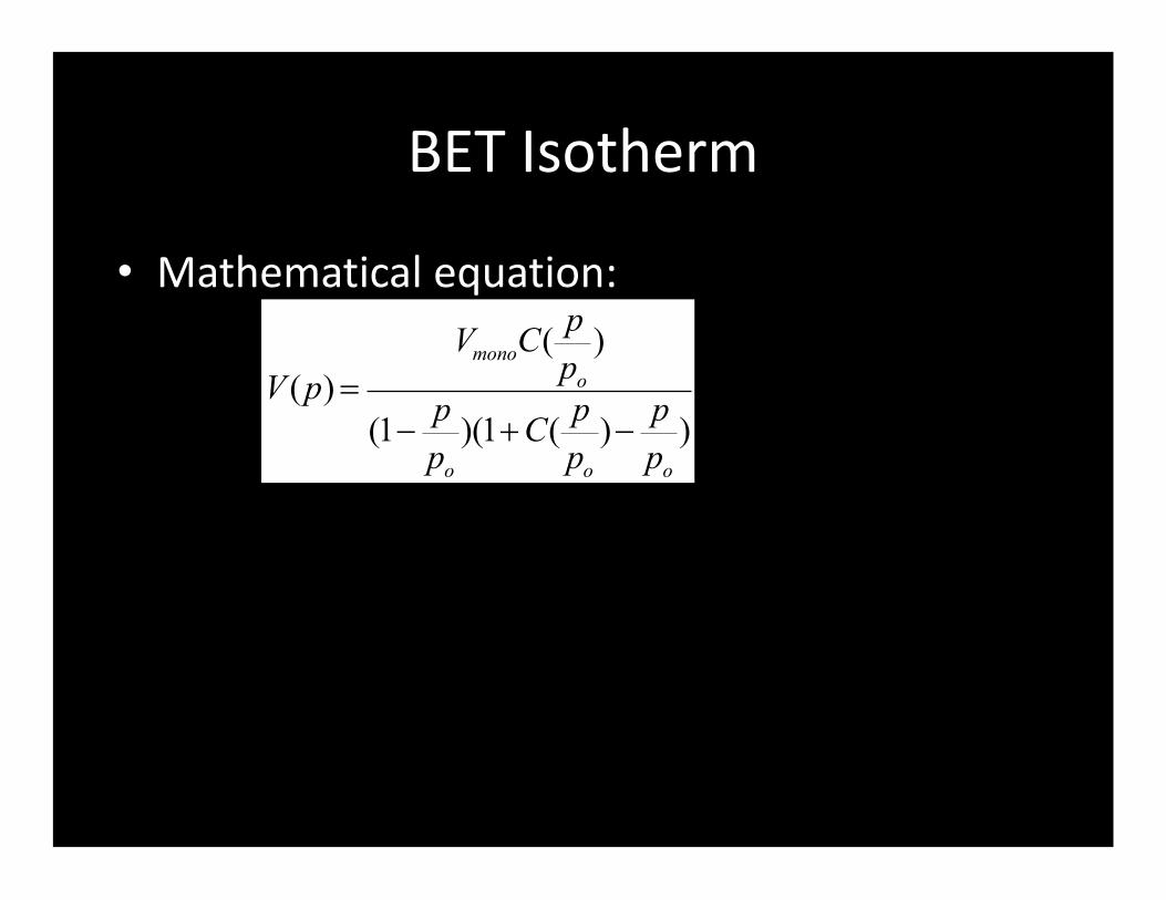
BET Isotherm

• Mathematical equation:

V (p) =

VmonoC(p

po)

(1-p

po)(1+C(

p

po)-p

po)