Final Report

Michigan Great Lakes Protection Fund Project

Grant Agreement Number 000530

Micrometeorological Measurements of Air-Water Exchange Rates of Persistent Bioaccumulative Toxicants in Lake Superior

September 2000 – June 2004

Judith Perlinger, Principal Investigator

Submitted 6/28/2004

Revised 9/14/04 Accepted 9/22/04

2

Abstract

Many persistent bioaccumulative toxicants (PBTs) have been shown to enter the Great Lakes primarily

through wet and dry deposition, where dry deposition is composed of gaseous- and particulate-phase

deposition. Aqueous PBTs are also capable of undergoing volatilization from lakes. Air-water exchange

has been shown to be the major component of this atmospheric component of the mass balances for many

PBTs. This component is typically estimated using the Whitman two-film model and appropriate

parameterizations. In this project, we developed a novel micrometeorological method for direct

measurement of air-water exchange of PBTs. The method utilizes diffusion denuders to rapidly collect

gas-phase PBTs upstream of a filter, where particulate PBTs are collected. PBTs collected in diffusion

denuders are transferred in carrier gas by thermal desorption to the cooled inlet of a high-resolution gas

chromatograph equipped with micro-electron capture detection for analysis. This analytical approach

presents advantages in terms of both performance and cost, and enables direct air-water exchange flux

measurements to be carried out on a time scale of three hours in Lake Superior. Results of concurrent

modified Bowen ratio measurements and Whitman two-film estimates of fluxes of selected PBTs in 2002

and 2003 in Lake Superior are presented and compared. Measured sensible heat fluxes were close to

mean monthly estimates from Lofgren & Zhu (1999). Gaseous concentrations of

α−hexachlorocyclohexane (α−HCH) and hexachlorobenzene (HCB) were frequently found at

concentrations greater than their respective method detection limits when samples were collected for two

or three hours, while those of the other target analytes typically were not. Recoveries of the surrogate

compound in field samples averaged 86 ± 24 % (RSD). The PBT concentration gradient at two heights

above the water surface, needed to compute the flux using the modified Bowen ratio, was great enough to

compute a flux using the modified Bowen ratio in 62 and 75 % of the cases for α−HCH and HCB,

respectively. High-volume air and water samples collected and analyzed by us contained concentrations

of PBTs were generally lower than those reported by the Integrated Atmospheric Deposition Network

(IADN) for Eagle Harbor, MI and Lake Superior, respectively. Whitman two-film flux estimates

computed from these concentrations also followed trends in Whitman two-film flux estimates reported by

the IADN Project. Diffusion denuder and high-volume gaseous concentrations were similar to one

another, although, not surprisingly, differences were observed during a 24-hour sampling experiment on

the R/V Lake Guardian between the (integrated) high-volume measurements and the (ca. 2- or 3-hour)

diffusion denuder measurements. The modified Bowen ratio flux results that were generated in this study

demonstrate that this novel micrometeorological approach is useful to determine the value of the fluxes

directly, with greater certainty and spatiotemporal resolution, and at lower cost than possible with the

Whitman two-film approach.

3

Introduction Since its inception in 1990, the Integrated Atmospheric Deposition Network (IADN) Project, as well as numerous other research projects, have utilized shore-based high-volume air sampling to measure gas- and particulate-phase PBT concentrations to estimate air-water exchange and depositional fluxes, respectively, of the chemicals. Air-water exchange represents a major source of some of the chemicals to the Great Lakes (or from them through volatilization), and the IADN project presently estimates the magnitude and direction of this flux using the Whitman Two-film Model (W2F Model) (Whitman 1923). Through funding of this project September 2000 – June 2004 by the Michigan Great Lakes Protection Fund (MI GLPF), technology developed by the Principal Investigator’s group provides an accurate, more rapid and inexpensive means by which to measure gas and particulate phase concentrations of PBTs and a direct, micrometeorological method for gaseous PBT flux quantification to/from surfaces including water (as opposed to an estimation). The specific objectives of this project were to (1) develop a modified Bowen ratio technique to measure air-water exchange rates of PBTs in Lake Superior; (2) compare direct measurements of air-water exchange rates with those estimated by the W2F Model; and (3) evaluate air-water exchange models by assessing the influence of meteorological (e.g., stability/instability of the atmospheric boundary layer) parameters on the exchange rates of PBTs in Lake Superior. This final project report documents the technology developed and the results generated to meet the project objectives.

Background Aqueous concentrations of PBTs continue to decrease in the Great Lakes, but concentrations in fish remain high enough to warrant fish consumption advisories. PBTs have strong sources from outside a Great Lake's watershed via atmospheric long-range transport and deposition, often by gas-phase deposition. For example, the 2000 LaMP for Lake Superior states that an estimated 82 - 95 % of polychlorinated biphenyl compound (PCB) loading and 80 - 100 % of dioxin/furan loadings occur via atmospheric deposition. The USEPA currently estimates fluxes and loadings of PBTs to the Great Lakes by monitoring atmospheric concentrations at IADN Master and Satellite stations located across the Great Lakes and computing PBT fluxes using the W2F Model. According to this model, the flux is estimated as:

−=

'HC

CkFlux Exchange Water-Air PBT awol (1)

where kol represents the overall mass transfer coefficient, Cw the aqueous PBT concentration, Ca the gas-phase PBT concentration, and H’ the dimensionless Henry’s law constant. The overall mass transfer coefficient kol is defined as the inverse sum of the partial mass transfer coefficient on the air side (ka) and the partial mass transfer coefficient on the water side (kw):

a

aa z

Dk ≡

w

ww z

Dk ≡ [cm/s] (2)

'111Hkkk awol

+= (3)

The value of the CO2 mass transfer coefficient (cm/h) has been parameterized by the following empirical equation: (Schwarzenbach et al. 1993)

64.110, 45.0

2uk COw = (4)

4

where 10u = wind speed (m/s) at 10 meters above the water surface. The mass transfer coefficient of chemical x is correlated to

2,COwk by: 5.0

,,2

2

−

=

CO

xCOwxw Sc

Sckk (5)

where Scx = Schmidt number of the chemical x. Because the Schmidt number is defined as the ratio of the kinematic viscosity to diffusivity, and the kinematic viscosity is dependent only on solvent, the ratio of diffusivities is found by cancellation of kinematic viscosity:

( )( ) x

CO

CO

s

CO

x

DD

DD

ScSc 2

22//

==νν

(6)

where ν = kinematic viscosity (cm2/s). The Wilke-Chang method, (Poling et al. 2000)is an empirical modification of the Stokes-Einstein relation, and is employed to determine the molecular diffusion coefficient as

( )

6.0

5.08104.7

mVTMsD

µφ−×

= (7)

where D = molecular diffusion coefficient of solute x in solvent S (cm2/s); φ = association factor of solvent S;

Ms = molecular weight of solvent S (g/mol); T = water temperature (K); µ = dynamic viscosity of solvent S (cP); Vm = molar volume of solute at its normal boiling temperature (cm3/mol). Considering the same solvent, S, for diffusion of substance x and the reference substance CO2, all terms except Vm can be cancelled. The Schmidt number ratio of x and CO2 can be expressed as below given the molar volume of CO2 is 29.6 cm3/mol (Poling et al., 2000).

6.0.,

6.292

2

== xm

x

CO

CO

x VD

DScSc

(8)

Substituting Equation (8) into Equation (5), the mass transfer coefficient kw,x (cm/h) for the diffusing substance x can be related to Vm,x and u10:

3.0,64.1

10

5.06.0,64.1

10

5.0

,, 6.2945.0

6.2945.0

2

2

−−−

=

=

= xmxm

CO

xCOwxw

Vu

Vu

ScSc

kk (9)

On the air side, the mass transfer coefficient of water, OHak2, (cm/s), can be described empirically as

(Schwarzenbach et al., 1993):

3.02.0 10, 2+= uk OHa (10)

and the mass transfer coefficient of diffusion of substance x, ka,x, is related to OHak2,

61.0

,

,,,

2

2

=

OHa

xaOHaxa D

Dkk (11)

where Da,x = molecular diffusion coefficient of compound x in air (cm2/s);

5

OHaD2, = molecular diffusion coefficient of water in air (cm2/s).

Fuller et al. modified an equation to describe the diffusion coefficient of solute x in solvent S, which is employed as:

( ) ( )[ ]23/13/15.0

75.100143.0

SdxdxS VVPM

TDΣ+Σ

= (12)

where T = water temperature (K); P = pressure (bar); Mx,S = inverse weighted average mass of solute x and solvent S = 2(Mx

-1 + MS-1)-1 (g/mol);

( )dVΣ = sum of diffusion molar volumes for compound constituents (cm3/mol).

In the ratio

OHa

xa

DD

2,

, , many terms cancel out,

( ) ( )[ ]( ) ( )[ ]23/13/15.0

,

23/13/15.0,

,

, 22

2 airdxdairx

airdOHdairOH

OHa

xa

VVM

VVMDD

Σ+Σ

Σ+Σ= (13)

According to the values from Poling et al. (2000),

( )airdVΣ = 19.7 cm3/mol and ( ) OHdV2

Σ = 13.1 cm3/mol

Mair = 29 g/mol and MH2O = 18 g/mol, and Equation (13) can be simplified as:

( ) ( )( ) ( )[ ]

( )( )[ ]23/13/1

5.0

23/13/15.0

23/13/15.0

,

,

7.19

29/1/13.85

7.1929/118/1

7.191.1329/1/1

2 +Σ

+=

+Σ+

++=

xd

x

xd

x

OHa

xa

V

M

V

MDD

(14)

Substituting Equation (14) into Equation (11), the mass transfer coefficient on the air side can be expressed in cm/s as:

( ) ( )( )( )

61.0

23/13/1

5.0

10,

,,

7.19

29/1/13.02.01561.0

2

+Σ

++=

=

xd

x

OHa

xaxa

V

Mu

DD

k (15)

In summary, with values for molecular mass and molar volumes for the compounds of interest, meteorological data such as water temperature (T) and wind speed (u10), and values for the concentrations of the compound in the air (Ca) and water (Cw), the flux of compound across the air-water interface is estimated. How representative are concentrations measured at the IADN Master Stations of over-water concentrations has been questioned by each peer review panel for the IADN (1997 and 2002), and the need for over-water measurements was emphasized. A key action of the Great Lakes Strategy of 2002 is to integrate the IADN with new regional, national, and international monitoring efforts and to evaluate the expansion of the IADN network to include new urban sites in order to determine urban sources. The 2000 LaMP for Lake Superior identifies three data gaps related to the research proposed here. Ambient monitoring data for pollutants of concern often lack the appropriate spatial and temporal scales to be able to quantify loadings to all water bodies and to calibrate and validate atmospheric transport and deposition models. The research proposed here allows relatively high spatial and temporal atmospheric sampling to be carried out. The LaMP recommends development of new techniques for direct air-water exchange measurements. The Lake Superior LaMP also states a need to collect concurrent air and water samples

6

for PBTs for W2F Model estimations of fluxes. However, because the direct method does not require aqueous-phase concentrations for flux determinations, this need is obviated. Conventional methods for PBT concentration and flux determination have additional limitations that cause uncertainty and bias, and the methods employed in the Principal Investigator’s group are not subjected to these limitations. The accuracy of W2F Model estimates of PBT fluxes has not been ascertained previously because a direct method for measurement of semi-volatile organic chemical (SVOC) fluxes to/from water has not been available. The known uncertainty of W2F Model estimates has been reported to be 50 – 7400 % (Hoff 1994, Hoff et al. 1994, Hornbuckle et al. 1994, Hoff et al. 1996, Bruhn et al. 2003). However, blow-on/blow-off of vapor-phase PBTs onto/from filters (and associated particulates) anterior to sorbent traps may cause bias in concentrations detected in the gas and particulate phases (McDow 1999). Because high-volume sampling is typically carried out for 24 hours, re-partitioning of collected gas phase PBTs and particulate-associated PBTs due to diurnal temperature and humidity variations may occur. These biases and uncertainties are minimized using the diffusion denuders for sample collection because filters are located posterior to diffusion denuders, and gas phase PBTs are rapidly (residence time = 0.05 seconds) stripped from the aerosol (defined as gas and particulate phases) in the diffusion denuder, and particles and their associated PBTs are trapped on the filter. In addition, using the diffusion denuder sample collection and analytical approach, adequate analyte mass is obtained in minutes to hours such that effects of temperature and humidity variations on re-partitioning during sampling can be minimized. In addition to the potential bias in concentrations measured in the vapor and particulate phases using conventional high-volume sampling, there are a number of limitations in the use of the W2F Model that are avoided by utilizing micrometeorological approaches for PBT flux measurement. First, the temperature-dependent Henry's law constant, a critical physicochemical property for estimating air-water exchange, is frequently not known as accurately as needed to estimate the small fluxes that are observed in the Great Lakes and elsewhere (e.g., Totten et al. 2002, Bruhn et al. 2003). This parameter is not needed for the micrometeorological flux measurement technique. Second, mass transfer coefficients of the PBTs in air and water are estimated empirically, and the parameterization used may or may not accurately account for important influences on the coefficients. For example, the parameterizations for mass transfer coefficients currently utilized by the IADN project do not account for impacts of surface films, bubbles, or sea spray, or reported increases at high wind speed (greater than ~10 m s-1) (Wanninkhof and McGillis 1999). The mass transfer coefficient parameterization utilized by the IADN project also assumes that an infinite and completely mixed mixing volume of air exists over the lake; the parameterization does not account for the effect of atmospheric stability in the surface layer. When the surface layer is stable, eddy diffusivity of air over the lake may drop two orders of magnitude within a few kilometers of the lakeshore (Lyons 1975), and this process may cause a significant decrease in the actual flux as compared to the flux estimated by the IADN (Honrath et al. 1997). Micrometeorological flux measurement techniques directly quantify effects of atmospheric surface layer resistances and high wind speeds, as well as those of surface films, bubbles and sea spray. Furthermore, meteorological and limnological conditions, the driving forces for mass transfer, can vary greatly over the time and space scales of measurements utilized in the W2F Model to estimate fluxes to lakes, and these scales are poorly represented in the current approach. For example, the IADN Project estimates air-water exchange fluxes based on concentration measurements of gas samples collected at an on-shore monitoring site on each lake and water samples collected off-shore. Often, these sample types are collected at different times/places, and water sampling frequency is typically much lower than air sampling frequency (e.g., annual or multi-annual vs. ca. two times monthly). Not only is it unlikely that on-shore measurements represent over-lake conditions due to the effects of atmospheric stability and turbulence (Honrath et al. 1997), aqueous concentrations may vary considerably in the interims in which measured concentrations are unavailable. In lakes and oceans, micrometeorological flux measurements

7

are carried out in situ in research vessels, on buoys, or on in-water towers. Also, because aqueous concentration measurements are unnecessary in micrometeorological flux measurement, error in flux estimation due to differences in air and water sampling frequency are avoided. In this project we developed analytical techniques to and a micrometeorological method for determining air-water exchange rates of PBTs, and carried out concurrent micrometeorological measurements and high-volume air and water sampling and analysis for PBT fluxes estimated using the W2F Model. Diffusion denuders were designed after those of Krieger and Hites (1992, 1993, 1994), fabricated, tested, and used to collect seven vapor-phase target PBTs in Lake Superior (Perlinger et al. 2004). The diffusion denuders are an integral part of a two-platform system designed to measure fluxes of PBTs to Lake Superior using the modified Bowen ratio approach (Perlinger et al. 2001, Doskey et al. 2002, Tobias et al. 2003). Gas-phase PBTs are collected in capillary tubes in diffusion denuders because they diffuse to the capillary walls rapidly under laminar flow conditions, where they sorb to the stationary coating inside the capillaries. Particles, which have much lower diffusivities, do not reach the capillary walls before exiting the denuder. A filter placed after a diffusion denuder in the flowpath can be used to collect particulate-phase PBTs, but the focus of the current project has been on collection and analysis of gas-phase PBTs. The multicapillary diffusion denuder consists of ca. 289 sections of commercially-available fused-silica capillaries sections in a Silcosteel-coated stainless steel tube. The capillaries are fused to one another and to the outer tube using polyimide resin, the same resin that is used to coat the outside of most commercial fused silica capillary columns. Thus, unlike the diffusion denuder design of Krieger and Hites, who used an epoxy to fuse the column sections together that cracked when heated, this diffusion denuder can withstand the same temperature conditions as the fused-silica capillary columns from which it is constructed.

Methods Chemicals. Individual target analytes were purchased from Accustandard (New Haven, CT) in concentrations of 100 µg/mL in isooctane (PCB Congeners 18, 30, 44, 52, 65, 101, 204) or methanol α-HCH, γ-HCH, HCB). Multiple component standards were then created using 99.9% pure hexane (Burdick & Jackson, Muskegon, MI) for trace analysis at or below the part-per-billion level as the solvent. PCB congener 65 was used as the surrogate standard, and PCB congeners 30 and 204 were used for internal standards. Diffusion Denuder Fabrication. Diffusion denuders consisted of a 5/8-in. OD × 25.5-cm stainless steel tube treated with Silcosteel® (Restek, Bellefonte, PA) containing 285 – 289 25-cm sections of 30 m × 0.53 mm × 5 µm film thickness Zebron ZB-1 100 % dimethylpolysiloxane capillary columns. Prior to cutting into sections, the 30-m capillary columns were conditioned at 330 °C for 4 hours with nitrogen carrier gas flow in a HRGC. PI2525 Pyralin® Polyimide Coating (HD Microsystems, Parlin, NJ) was used to cement the capillary columns together in the stainless steel tube. Following diffusion denuder assembly, the polyimide resin inside the diffusion denuder was hardened using a detailed curing process recommended by HD Microsystems. The intent of the curing process was to avoid blistering and creation of voids in the polyimide resin during hardening while protecting the stationary phase within the capillary columns from oxidation. Thermal desorption of the diffusion denuders immediately following the curing procedure demonstrated that the diffusion denuders emitted compounds that were electron-capture sensitive. The addition of a post-cure procedure to immediately reduce the liberation of these compounds resulted in clean chromatogram runs of the fabricated diffusion denuders. Analytical System. Analyses were performed on an Agilent Technologies 6890A Plus Series HRGC-microECD. The 6890A HRGC is equipped with a Programmable Temperature Vaporization (PTV) inlet with liquid nitrogen cryogenic capability made by Gerstel, Inc. (Baltimore, MD) and purchased from

8

Agilent with the HRGC. The analytical column used for separation of target analytes is a DB-XLB, 60 m × 0.25-mm ID × 0.25-µm film thickness (Agilent Technologies-J&W Scientific, Folsom, CA) capillary HRGC column. The carrier gas was helium at a flow rate of approximately 2.1 mL min-1, which yielded a linear velocity of 36 cm sec-1 in constant flow mode. Nitrogen at a flow rate of 60 mL min-1 was the makeup gas for the microECD. Direct thermal desorption of analytes into the HRGC was carried out after modifying the 6890A HRGC and fabricating a thermal desorption unit (TDU) and a hot gas spike apparatus as described below. Modification of the 6890A HRGC for Thermal Desorption of Analytes from Diffusion Denuders. Modification of the 6890A HRGC carrier gas lines was necessary prior to interfacing with a TDU because the PTV Inlet was factory-equipped with a septum head for liquid injections. The septum purge line and carrier gas supply line were cut from the original septum head weldment on the HRGC, and the weldment was removed. The septum purge outlet was capped and the septum purge line was joined to the carrier gas supply line. Combining the septum purge and carrier gas lines resulted in approximately 5 mL min-1 higher total carrier gas flow than indicated by the HRGC’s electronic pressure control system, but did not negatively affect the operation of the instrument. The carrier gas line was then routed into the thermal desorption unit. A direct interface unit (Gerstel, Baltimore, MD) provided transfer of analytes through a heated transfer line from the diffusion denuder fitting in the thermal desorption chamber of the TDU to the PTV Inlet. This modification of the carrier gas lines allows both TDU and HRGC flow to be controlled by the 6890A HRGC EPC system. Thermal Desorption Unit. A thermal desorption unit was designed by us and constructed by CDS Analytical (Oxford, PA). The unit consists of an insulated tube heater connected to a controller that enables precise temperature regulation. Carrier gas flow through the unit is connected directly to the Gerstel direct interface. The transfer line that connects the thermal deosrption chamber to the Gerstel direct interface consists of a 0.53-mm ID, 0.70-mm OD deactivated fused silica capillary that extends through the Vespule ferrule into the PTV Inlet. The transfer line heater was designed and constructed so that it rests inside the recess at the top of the PTV Inlet rather than covering the entire surface, and consists of a 6-inch section of ½-inch OD, 3/8-in. ID stainless steel tubing. The tubing is wrapped with heat tape, and a thermocouple (THERMOCOAX, Alpharetta, GA) is used to monitor the temperature of the transfer line. The temperature of the heat tape was controlled using a variable transformer. Second, modifications were made to the top cover of the PTV Inlet to provide circulation for cooling air through the internal area of the cover of the inlet while the transfer line heater is at elevated temperatures. A 1/16-inch cooling airline was installed through a hole drilled in the top of the inlet, while a second hole was drilled to provide a route for the cooling air to circulate within and out of the cover. Hot Gas Spike Apparatus Fabrication and Use. The hot gas spike apparatus consists of 1/8- and 1/16-inch Silcosteel tubing connected to a 1/16-in. tee fitted with a septum injector nut (VICI Valco, Houston, TX), a two-way valve for nitrogen carrier gas, and a metering valve. The tubing and tee were wrapped first with glass tape and then with heat tape controlled by a variable transformer. The diffusion denuder to be spiked is connected to the apparatus with a Swagelok fitting downstream of the heated zone, and is enclosed in a cooling jacket consisting of 3/16-inch copper tubing with cold tap water flowing through it. All heated zones and fittings received Silcosteel treatment prior to use. To optimize standard transfer to the diffusion denuder, the apparatus was designed with sufficient volume to avoid expansion of the carrier solvent hexane into the dead volume in the tee upon vaporization. The injection point within the tubing is located far enough downstream of the tee that expansion of solvent occurred in the tubing volume only, not in the dead volume of the tee. In this way, carry-over of standards from spike to spike is prevented.

9

Diffusion denuders are spiked in a fume hood as follows. Standards in ca. 3 µL hexane are spiked with a long-needle 10-µL syringe (Hamilton, Reno, NV) into the Hot Gas Spike Apparatus heated to 260 °C at a nitrogen gas flow rate of 500 mL min-1. The volume of solvent delivered is determined from solvent density and the difference in weight of the syringe containing standard and that after the standard has been spiked into the apparatus. During spiking, diffusion denuder temperature is held at 13 - 15 °C. On one occasion, a second diffusion denuder was connected in series with a diffusion denuder being spiked. Upon thermal desorption, the second diffusion denuder contained no detectable standard. Analyte Desorption from Diffusion Denuder and HRGC Analysis. Pfannkoch and Whitecavage (2000) employed stopped-flow techniques for thermal desorption of sorbent tubes packed with Tenax-TA and tubes containing fresh peppers. Stopped-flow thermal desorption involves the reduction of column flow to the lowest value possible during thermal desorption to reduce the amount of water transmitted to the capillary column. For a thermal desorption run, a Tenax-TA-packed inlet liner is used in the PTV Inlet. The diffusion denuder is oriented in the TDU oven such that it is back-flushed during thermal desorption, and is connected at the top of the TDU oven with a Cajun fitting using Teflon ferrules and at the bottom of the TDU oven with a custom 5/8- to 1/16-inch reducing fitting. The following procedure describes the steps required for a 101-min analysis of a diffusion denuder using a detector temperature of 300 °C, transfer line temperature of 260 °C, a PTV Inlet temperature of 5 °C, and a desorption flow rate of 750 mL min-1 followed by a typical analytical run. Initial conditions: HRGC oven temperature = 100 °C; inlet mode = split, 500 mL min-1; PTV Inlet temperature = 200 °C; (1) heat TDU oven to 70 °C, set column flow to 0.8 mL min-1 and total flow to 500 mL min-1 to purge water from the diffusion denuder; (2) after 10 minutes, cool the PTV Inlet to 5 °C; (3) initiate thermal desorption by increasing the TDU oven temperature to 230 °C; (4) when TDU oven temperature reaches 230 °C, set total flow to 750 mL min-1; (5) after 18 minutes, turn off the TDU oven and transfer line heaters, set total flow to 6.0 mL min-1; (6) set PTV Inlet temperature to 10 °C and increase by 5 °C every 30 sec to 105 °C; at 105 °C set column flow to 2.1 mL min-1 and hold for 10 minutes to purge the HRGC column(s) of water; (7) begin HRGC analysis. The HRGC method used for analysis is: inlet temperature = 320 °C for duration of run; inlet mode = splitless; split flow = 30 mL min-1 after 6 min; column flow mode = constant flow, 2.1 mL min-1; HRGC oven temperature: 100 °C for 6 min, 1 °C min-1 to 240 °C, 10 °C min-1 to 280 °C, hold at 280 °C for 20 min; detector temperature = 300 °C; detector makeup gas = nitrogen, 60 mL min-1. Calibration Using Internal Standards. Calibration of the HRGC for diffusion denuder was carried out by plotting the ratio:

IS

ISA

AMA

y×

= (16)

where AA = area of analyte peak, MIS = mass of the internal standard injected into the gas chromatograph, and AIS = area of the internal standard peak versus x, where x = MA, the mass of analyte in the standard injected into the gas chromatograph. In analysis of PBTs in diffusion denuders, the mass of standard injected corresponds to that injected into the diffusion denuder using the hot gas spike apparatus. A second-order polynomial fit of the plot of y vs. x of the following form was used to describe the non-linear variation in detector response with analyte mass at low mass:

10

cbxaxy ++= 2 (17) Calculation of Analyte Mass in Sample. The mass of analyte in a sample (MA) was calculated from the calibration curve. For a given response of analyte and internal standard in the sample, the corresponding mass in the sample was computed by finding the x root values of the second-order polynomial according to the following expression. One of the two values is the useful value.

aycabb

x2

)(42 −−±−= (18)

For analysis of solvent extracts, a similar approach was used except a power equation was used to fit y vs. x of the form y = mxb. This approach differs from the standard approach in which response factor values are computed from linear regressions of analyte area vs. mass. However, the approach used is warranted given the non-linear response of our ECDs in the concentration range of interest, and provides more accurate values of analyte mass. Micrometeorological Measurement of Fluxes. We have fabricated, tested, and utilized energy balance sampling platforms for large and small research vessels to directly measure fluxes of the target PBTs in Lake Superior. The micrometeorological principle we utilize in the flux measurement is expressed in the modified Bowen ratio equation (Wesely 1988), which assumes that the mass transfer coefficient of any two scalar quantities between two heights in the atmospheric surface layer is identical. This assumption has not been disproven within the precision of simultaneous measurements of two scalars (Panofsky and Dutton 1984). In this case, sensible heat flux is the scalar whose flux is measured by direct covariance. The modified Bowen ratio is the product of the sensible heat flux and the ratio of the difference in PBT concentrations measured at two heights above the air-water interface divided by the difference in temperature at the two heights.

PBT Air-Water Exchange Flux =T

PBTc

H

p

s

∆∆ ][

ρ (19)

where Hs is sensible heat flux, measured as the average of the product of the variances in temperature and vertical wind speed measured at 20 Hz, ρ is air density, cp is the specific heat capacity of air at constant pressure, T is air temperature, and ∆ symbolizes the difference in measured PBT concentrations at two heights above the water surface. Ship movement during sampling induces artificial winds at the sonic anemometer that is corrected for according to methods developed by Edson et al. (1998). We have carried out flux measurements on the R/V Lake Guardian and Michigan Tech’s research vessel R/V Agassiz in Lake Superior on eight occasions. Micrometeorological sampling was carried out onboard the R/V Lake Guardian on three occasions utilizing our upper and lower energy balance platforms for large research vessels (Figure 2). On the R/V Lake Guardian, the upper platform is attached to the mast in the ship’s bow using a steel collar and bolts that tighten the collar at a height of approx. 5.0 m above the hotel deck (approx. 8.5 m above the water surface). At this location, mean flow tilt angles are expected to be approximately 5 °, which has been considered to be acceptable for similar work (Edson et al. 1991, Oost et al. 1994, Fairall et al. 1997). The lower platform consists of a hollow aluminum 3” × 3” × 6 m pole that is guided towards the water surface in an L-shaped steel guide that can be bolted to the ship’s bow. The pole is fastened to the steel guide during sampling and retrieved to change diffusion denuders. Sampling was also carried out on Michigan Tech’s 36-foot R/V Agassiz using a 10-m telescoping mast donated by KSTP Weather Station

11

(Minneapolis, MN) and refurbished by us and utilizing our upper and lower energy balance platforms for small research vessels. A diffusion denuder spiked with surrogate standard PCB 65 for PCB and pesticide analytes and loaded into an aspirated sampler housing was installed on the upper platform for sampling on either vessel. A second diffusion denuder in an aspirated sampler housing and spiked with surrogate standard was installed on the lower platform located approximately at approx. 1 m above the water surface. Micrometeorological PBT flux measurements were carried out at various locations as shown in Table 1 and Figure 3. For these measurements, PBT sampling was carried out at an average flow rate of 13 L min-1 for two or three hours. The difference in concentration of target PBTs in Eqn. (18) is computed utilizing the concentrations measured in the diffusion denuders on these platforms. The difference in temperature in Eqn. (18) is computed from temperature measurements at the upper and lower platforms. These temperature measurements are carried out using Model ASPTC thermocouples in aspirated sampler housings (Campbell Scientific, Inc., Logan, UT). The signals from these thermocouples are recorded by the CR5000 data logger. In Eqn. (19), the sensible heat flux, Hs, is computed as:

''TwcH ps ρ= (20) where ρ is air density, cp is the specific heat capacity of air at constant pressure, w’ is the variance in vertical wind speed measured at 20 Hz, T’ is the variance in air temperature measured at 20 Hz, and the overbar indicates the average of the product of the variances over the measurement period. Windspeed and temperature are measured using a Model CSAT3 (Campbell Scientific, Inc., Logan, UT) sonic anemometer and a finewire thermocouple (FW05, Campbell Scientific, Inc., Logan, UT) for the determination of sensible heat flux. All signals (three-dimensional (3-D) windspeed, thermocouple signal, internal sonic anemometer temperature) are recorded on the CR5000 data logger. These signals are corrected for axial acceleration using an attitude and reference system (Edson et al. 1998). Model AHRS300CB, Crossbow Technology, Inc. (San Jose, CA) accelerometer, which measures and transmits roll, pitch, and heading (azimuth) angles to the CR5000 datalogger. The accelerometer is completely enclosed inside a plastic container and fastened to the arm of the sonic anemometer. High-volume Gaseous and Aqueous Concentration Measurements. We utilized or modified existing procedures to determine gaseous and aqueous concentrations of the target analytes. For the gas-phase concentration measurements, we utilized the IADN Project procedures (Basu 1995, 2000, USEPA and Canada 2001) with specific procedures as described in detail by Zhu (2003). For aqueous-phase concentration measurements, we utilized procedures of the IADN Project (Basu 2000) with specific procedures as described in detail by Zhu (2003). High-volume air sampling was carried out for 24 hours at an average flow rate of 600 L min-1 (Table 1). Water samples were collected from the upper 5 m of water in the locations shown in Table 1. Volumes of 150 L and 220 L were collected in the Fall 2002 and Spring 2003 samples, respectively.

Results and Discussion Functioning and Cost of Diffusion Denuders and Thermal Desorption Technique. The diffusion denuders and thermal desorption method developed in this project proved useful in collection, storage, and analysis of two of the seven target analytes shown in Table 1, and if breakthrough is not a problem, the samplers and methods developed here will be useful for determination of concentration of many more PBTs such as the additional PCB congeners not analyzed in this project and polybrominated diphenyl ethers. The

12

diffusion denuders exhibited no cracking or leakage even though they have been utilized in hot gas spiking and sample collection repeatedly over the course of the project. Of the 28 diffusion denuder samples collected in the field (Table 1), the average recovery of the surrogate standard PCB 65 was 80 ± 21 % (RSD). These samples were stored refrigerated from 6 – 27 months. Higher recovery (86 ± 24 % (RSD)) was observed in samples after storage for six months or less, suggesting that the target analytes are subject to degradation processes within diffusion denuders during storage. However, the procedure for spiking was carried out by different individuals in the two sample sets, suggesting that a different spiking procedure may have been followed for the first set of samples as compared to the second set of samples. The effect of storage time over a one-year period is under evaluation at this time. The adequate average recovery indicates that, at least for the surrogate injected into diffusion denuders prior to sample collection, out-competition by water or other organic compounds for sites on the polydimethylsiloxane coating inside the capillaries is not a problem. We estimate that cost savings of 70 % can be obtained using diffusion denuder sampling and thermal desorption analysis as compared to conventional sampling/analysis methods based on a per-sample cost of $1,200 for high-volume air samples (I. Basu, IADN Project, personal communication). If the chromatography columns used to fabricate diffusion denuders can be purchased in bulk at reduced rate, the cost savings will be greater. For example, for a portion of the diffusion denuders we fabricated, we were able to obtain 50 chromatography columns at a savings of 50 % from Phenomenex, Inc. Sampling time was reduced from 24 hours using high-volume sampling to 3 hours over Lake Superior for the analytes detected. Because no sample processing is required prior to sample analysis, turn-around time on such analyses is significantly lower. For example, to process a batch of six high-volume air or water samples requires 12 – 15 days. This processing time is eliminated using thermal desorption extraction of analytes into the gas chromatograph. Furthermore, since no XAD resin or solvents are used, there is no waste generated through PBT measurement. The diffusion denuders are re-useable. As of this time, we do not know the lifetime of our diffusion denuders as they have exhibited no sign of failure. Field Sampling. As shown in Table 1 and Figure 3, our field sampling was carried out in Summer and Fall in 2002 and Spring 2003 on or near the Keweenaw Peninsula. Sampling on the Keweenaw Peninsula was carried out at the IADN site in Eagle Harbor, MI. When possible, this sampling was carried out on dates corresponding to sample collection dates of the IADN Project. High-volume air samples were also collected at HN050 during the April 25th-27th event on the R/V Lake Guardian. Micrometeorogical PBT flux measurements were carried out at SU17, HN050, and EH050. Water samples were collected at HN050 and EH050. Sensible Heat Fluxes. Sensible heat fluxes required for PBT flux determination (Eqn. 19) should be corrected for platform motion, but could not be for these data due to lack of availability of required input data, as indicated in Table 1 (Notes 1 and 3). For the April 25th-27th cruise, all necessary data were available to carry out motion correction, but the sonic anemometer malfunctioned during part of the sampling event such that some of the sensible heat flux data had to be omitted from the calculation. The remaining data exhibited greater scatter than that obtained during other sampling events, and these data were not corrected for platform motion. In general, platform motion less than that in oceanic measurement of trace gas fluxes, so the corrections can be expected to be of less benefit relative to the error that is introduced in platform motion correction. Values of sensible heat fluxes averaged for each of the individual sampling events and not corrected for platform motion (Table 11) are compared with mean monthly averages of sensible heat flux estimated by Lofgren & Zhu (1999, 2000) in Figure 4. The estimates of mean monthly sensible heat flux are based on AVHRR data and meteorological data from locations surrounding Lake Superior. The agreement between the measured and estimated sensible heat fluxes gives validity to each approach for determining the values, at least for the Spring, Summer, and Fall seasons in which they are compared in the figure.

13

Instrument Detection Limit (IDL) and Method Detection Limit (MDL) Values. IDL and MDL values were determined for analysis of PBTs in high-volume air and water samples and for analysis of PBTs in diffusion denuders. For high-volume air and water samples, IDL values were computed as two times the relative standard deviation in five replicates of the lowest standard containing all analytes that produced signals greater than two times the peak-to-peak noise level of the baseline. MDL values for high-volume air and water sampling were computed as two times the relative standard deviation in four spikes of surrogate PCB 65 in lab blanks for air and water. In Table 3, IDL and MDL values are presented as picograms in the volume of hexane injected into the gas chromatograph, and converted to their concentrations in typical volumes of air and water collected. For PBTs collected using diffusion denuders, MDL values were computed as 3.365 times the relative standard deviation in three hot-gas spike standards of target PBTs containing masses equal to approximately five times their IDL values. Ideally, MDL values would have been computed from masses in five replicate samples of ambient air such that effects of the sample matrix (water content, organic compound content) could be taken into account. Setting up five parallel sample trains in order to obtain five replicate samples of ambient air is a major on-taking and will be undertaken in the future. Although the MDL values presented in Table 3 for high-volume air, water, and diffusion denuder sampling were computed slightly differently as described above, they can be compared in order to understand gross similarities and differences. On a per-picogram basis, MDL values for high-volume air and water sampling are similar to diffusion denuder sampling. On a concentration basis, however, because larger volumes of air are collected in the former case, MDL values are lower by one to two orders of magnitude for them than for sampling using diffusion denuders. When the MDL values for diffusion denuder sampling (on a concentration basis; last column in Table 3) are compared with concentrations of the target analytes measured in air using high-volume sampling in Fall 2002 and Spring 2003 (Tables 4 and 5), it becomes apparent that some target analytes were present at concentrations too low to be detected using the diffusion denuder sampling and analysis technique. Two compounds, α-hexachlorocyclohexane (α-HCH) and hexachlorobenzene (HCB) would be expected to be detected in diffusion denuder samples based on the concentrations determined using high-volume sampling. These two compounds were indeed most frequently detected in diffusion denuder samples (Tables 8 and 9), supporting the same conclusion as found for the surrogate PCB 65, that water or additional background organics do not outcompete target analytes for the polydimethylsiloxane coating in the capillaries. The compounds that were expected to be detected were detected, whereas the compounds that were not expected to be detected were not. Because α-HCH and HCB were most frequently detected in diffusion denuder samples, they will be discussed in more depth than the other analytes in the following. Complete analysis of all high-volume air and water results, including comparison with available IADN Project results, can be found in the thesis of Zhu (2003). Gaseous Concentrations Determined by High-volume Sampling. Gaseous concentrations measured by high-volume air sampling in Fall 2002 and Spring 2003 are reported in Tables 4 and 5, respectively. It should be pointed out that during Fall 2002 of this project, high-volume gaseous concentrations of target analytes were carried out over land at the IADN site in Eagle Harbor, whereas in Spring 2003 these concentrations were measured over water. Gaseous concentrations for α-HCH and HCB are lower in Spring 2003 than in Fall 2002 while those of γ-HCH and four PCB congeners are higher in Spring 2003 than in Fall 2002. For the comparison of gaseous concentrations of α- and γ-HCH, HCB, and PCB 18, 44, 52, and 101 measured in this project with historical data, we acquired the seasonal data for the IADN Eagle Harbor

14

site from 1990 to 2000 from data manager C. Audette of the IADN Project. Gaseous concentrations of α-HCH and HCB from 1990 through Fall 2002 and Spring 2003 are shown in Figures 5 and 6, respectively. It should be pointed out that the average seasonal concentrations shown in Figures 5 and 6 for Spring 2003 are based on four measurements carried out at two locations in Lake Superior during one 48-hour sampling event (Table 1). Concentrations of α-HCH in samples collected at SU17 on 4-25-03 were higher than those collected on 4-26-03 at HN050. This may be due to a change in air mass sampled at the two locations and times, as suggested by the order of magnitude increase in the temperature gradient being measured simultaneously by the micrometeorological system (Table 11) and a change in wind direction from north-northwest to southerly. After 22.5 hours had passed since the beginning of sampling on 4-25-03, this temperature gradient jumped, and as discussed later, this temperature gradient jump was accompanied by changes in the concentration profiles of α-HCH and HCB measured using diffusion denuders. The averaged Spring 2003 high-volume gaseous concentrations may therefore be biased because they do not account for inter-season variability. Over-land measurements carried out by the IADN Project at Eagle Harbor, MI demonstrate that in spring, α-HCH increased to 400 pg/m3 in 1992 and declined thereafter to approximately 50 pg/m3 in 2000 (Figure 5). The declining trend in α-HCH concentration is likely due to the ban of technical HCH in 1978 (Buehler et al. 2002). Similar to the spring season, the fall α-HCH concentrations appear to decrease to approximately 50 pg/m3 in 2000, but the range of the decrease is not as marked as that of the spring concentrations. From our over-lake measurements, α-HCH in Spring 2003 was slightly lower at 18 pg/m3 compared to 23 pg/m3 over-land in Fall 2002. Eagle Harbor γ-HCH concentrations in spring exhibited a similar increase in concentration as α-HCH to 150 pg/m3 in 1992 and then decreased dramatically the following year and remained roughly constant at 25 pg/m3 through 2000. However, there is a notably greater range in the seasonal concentrations of γ-HCH as compared to both the spring and fall α-HCH concentrations (data not shown). Our over-land measurements of γ-HCH concentration in Fall 2002 and our over-lake Spring 2003 measurements also exhibit similar concentrations as the most recent IADN data, having values of 14 pg/m3 in Fall 2002 and 33 pg/m3 in Spring 2003. The gaseous concentrations of HCB at Eagle Harbor show no decreasing trend during 1990-2000 and varied between 50 and 150 pg/m3 (Figure 6). Our over-land measurements in Fall 2002 and over-lake measurements in Spring 2003 are in agreement with or are lower than this concentration range at approximately 50 pg/m3 and 28 pg/m3, respectively. The Eagle Harbor gaseous concentration for the four PCB congeners maintained concentrations between 1 and 30 pg/m3 during the past decade. Our over-land and over-lake PCB measurements are of the same magnitude as the historical data. It is interesting that some of these semi-volatile organic chemicals exhibit higher concentration in one season than in the other. Whether or not these differences actually can be concluded from the data depends on whether concentrations are statistically different given the variability in the concentrations measured and their uncertainties. For the IADN Project data, these factors are presently not available. Minimum/maximum values are the only surrogate measures of uncertainty available for the IADN data. They should represent maximal uncertainty. Ignoring the maximum/minimum values as a means of distinguishing differences for the moment, the IADN Project data show that, for eight out of ten years the gaseous concentration of α-HCH was higher in fall at Eagle Harbor than in spring. The over-land average concentration in Fall 2002 was also slightly higher than our over-water measurement in Spring 2003. The gaseous concentrations of γ-HCH were higher in spring than in fall in all ten years. Our over-land measurements in Fall 2002 were lower than those in Spring 2003 for γ-HCH. For six out of ten years of the IADN Project dataset, the HCB concentration in fall were higher than those in spring. For seven out of ten years of the IADN Project dataset, the gaseous concentration of PCB 44 was higher in spring than in fall. For six out of ten years for PCB 18 and PCB 52 and for five of ten years for PCB 101, the gaseous

15

concentrations in spring were higher than those in fall. In our measurements, the gaseous concentrations for all four PCB congeners were higher in Spring 2003 than those in Fall 2002. High concentrations in Spring were also reported by Hornbuckle et al. (1994) in 1992 at Eagle Harbor and on the southeastern shore of Lake Superior near Sault Ste. Marie by Monosmith (1993). There are numerous possible explanations for seasonal differences in concentrations and for differences observed between our data and the IADN Project data. For all compounds, differences observed between our measurements and IADN Project measurements for α-HCH may be the result of different analytical labs having carried out the measurements. However, the agreement between our Fall 2002 Eagle Harbor measurements of γ-HCH and HCB concentration with the previous data suggest this is not the case for any of the analytes, especially considering that α-HCH is lower in Fall 2002 than in Spring 2003 in our measurements but that the IADN Project data exhibits a similar decreasing trend whereas the other analytes do not. Buehler et al. (2002) reported a half-life of 3.5 years for α-HCH based on the same 8 years of IADN data. Based on this half-life, a concentration of 34 pg/m3 should have been measured by us in Fall 2002. This is slightly higher than the range measured by us (avg. = 23; range = 15 - 30 pg/m3). However, the air that was sampled at the second station during the 48-hour sampling event in Spring 2003 may have been depleted of α-HCH as discussed in further detail with respect to atmospheric stability below. Previously, an effect called the “Early Spring Pulse” (Hornbuckle et al., 1994; Gouin et al. 2002) has been hypothesized to explain seasonal variations in concentration in terrestrial environments. The phenomenon has been hypothesized to occur when there is accumulation of PBTs in snowfall during the winter. As the snow melts in spring, PBTs volatilize and/or are transported from regions where they are volatilized from snow. After budding of leaves occurs in the forest, the leaves rapidly take up the PBTs, diminishing the local gaseous concentrations, creating the tail of the pulse. Trends with temperature are not statistically significant when errors are too large, however. Wania et al. (1998) noted that in all studies of α-HCH with a large number of samples, temperature explained none or a very minor fraction of the variability in the gaseous concentration, while the gaseous concentrations of γ-HCH were more strongly correlated with atmospheric temperature with a correlation coefficient (R2) of 0.11-0.75. Some researchers (Eisenreich et al. 1983, Hillery et al. 1997) noted that gaseous concentrations of PCBs are lower in the colder winter months and higher in the warmer summer months. Hillery et al. considered atmospheric temperature to be the predominant effect on gaseous concentrations of PCBs compared to wind speed, wind direction, and time (yearly variation). By comparing the gaseous concentration of ΣPCB, Buehler et al. (2001) also found that atmospheric temperature controlled most of the variability at two sites studied. This temperature domination was explained thermodynamically using the Clausius-

Clapeyron equation: constRT

HP +

∆−

=ln , where P is the partial pressure in bar, T is the atmospheric

temperature, K, ∆H is the heat of vaporization in J/mol, and R is the gas constant. In the region where our samples were collected, atmospheric temperature in fall is generally higher than in spring. However, although α-HCH and HCB gaseous concentrations were higher in fall than in spring in most years as might be expected according to the Clausius-Clapeyron expression, for some PCB congeners and for γ-HCH, the opposite concentration trend was observed, suggesting that temperature may not control concentrations for these species. A different factor likely explains the observed higher concentration in spring for γ-HCH. This compound is one of the top ten insecticides currently used in central Canada for the protection of livestock, crop seed, and poultry. It is likely higher in concentration in spring rather than fall in the Lake Superior airshed due to transport from central Canada, as supported by the recent analyses of Li et al. (2003), Ma et al. (2003, 2004a, 2004b), Shen et al. (2004), and Buehler et al. (2004). Ma et al. (2004b) reported a strong association of spring average air concentrations of HCHs, HCB, and two low-molecular weight PCBs around the Great Lakes with the North Atlantic

16

Oscillation (NAO). The authors explain the association by noting that, in the 1990s, western and northwestern North America experienced warmer-than-normal springs, enhancing volatilization of the compounds from reservoirs accumulated during past and present use. Atmospheric flows associated with the NAO then transported the compounds from source regions to downwind locations including the Great Lakes. Inter-annual fluctuations of the concentrations of the POPs correlated significantly with the 1000-500 hPa thickness of the atmospheric surface layer (ca. lowest 5 km) to the west of the Great Lakes and changes in zonal wind over the western United States. Additional factors besides temperature, chemical usage, or the NAO may partially explain why our over-water values of (α-HCH and) HCB concentration are lower and γ-HCH and PCB concentration are higher in Spring 2003 than the most recent measurements of concentration at Eagle Harbor in Fall 2002 by us. Because the concentration values are averages of two duplicate measurements carried out during only one 48-hour over-lake sampling event, the difference observed may be a result of over-land vs. over-lake measurements and an affect of atmospheric stability. As mentioned earlier, a large over-water temperature gradient was observed during a part of the collection of the second duplicate samples at HN050 (Table 11) indicating that during that period, a stable atmosphere was sampled, which may have been low in concentration of (α-HCH and) HCB and high in concentration of γ-HCH and the PCBs compared to the previous fall. Especially in spring, advective transport across water surfaces may cause development of an internal boundary layer due to the temperature difference between the lake and the atmosphere that may either promote or hinder air-water exchange depending on the extent of disequilibrium between this layer and the surface water. The surface water may furthermore be subject to additional sources of PBTs or be depleted of them through upwelling, another source of potential disequilibrium. As a result, analyses and models that do not account for stability of the atmospheric and water surface layers such as those presented by Ma et al. (2004a, 2004b) will not be able to accurately predict air-water exchange within these layers. This approach describes stability in the lowest ~5 km of the atmosphere, whereas effects of a cool lake surface on atmospheric stability occur in the lowest ~1 km or less of the atmosphere (Lyons, 1975). Aqueous Concentrations of PBTs. Historical data of aqueous concentrations of the seven target PBTs were obtained from IADN reports from 1996 to 1998. Specifically, in 1996, the aqueous concentrations of α- and γ-HCH and HCB in Lake Superior were collected by the USEPA R/V Lake Guardian cruise of 1996 and analyzed by USEPA GLNPO; CCGV Limnos cruise of spring and summer, 1996 and analyzed by EC NWRI, CCGV Limnos cruise of spring and summer 1996 and analyzed by EC EHD. The aqueous concentrations of PCBs 18, 44, 52, and 101 in Lake Superior were collected by the USEPA R/V Lake Guardian cruise of 1996 and analyzed by US EPA GLNPO. In 1997, the aqueous concentrations of α- and γ-HCH, HCB in Lake Superior were from EHD cruise (CCGV Limnos) for Spring and Summer 1997 and analyzed by NLET, under contract to Maxxam Analytics, CCGV Limnos cruise of spring and summer 1997 and analyzed by MSC, USEPA R/V Lake Guardian cruise of 1997 and analyzed by USEPA GLNPO, CCGV Limnos cruise of spring and summer, 1997 and analyzed by NWRI. The aqueous concentrations of PCBs 18, 44, 52, and 101 in Lake Superior were collected by theUSEPA R/V Lake Guardian cruise of 1997 and analyzed by the USEPA GLNPO. The historical data for the annual aqueous concentration in 1996 and 1997 and our measurements in Fall 2002 and Spring 2003 for the target analytes are presented in Tables 6 and 7 and shown in Figures 7 and 8. Unlike historical data for gaseous concentrations, the IADN data present neither the variability in the concentrations measured and their uncertainties nor minimum/maximum values. From Figure 7, it can be seen that the aqueous concentrations for α-HCH decreased approximately five times from approximately 2 ng/L to 0.38 ng/L from 1996 until 2003. Similarly, the aqueous concentrations for γ-HCH decreased approximately four times from 0.44 ng/L to 0.11 ng/L from 1996 until 2003. Some fraction of these decreases may be to due spatial variability in concentration. Although 90-95% of γ-HCH can be removed by microbial action within 12 weeks in the presence of sediment and river water (Rapaport and Eisenreich

17

1988), its aqueous concentration is still high, and α-HCH can be formed from metabolism of γ-HCH (Rapaport and Eisenreich 1988). Compared to α- and γ-HCH, Figure 8 shows that the aqueous concentrations of HCB and each of the four PCBs increased compared to seven years ago. The aqueous concentrations of HCB and four PCBs are lower than α- and γ-HCH which have concentrations of approximately 3.5 to 30.7 pg/L, respectively. Though PCBs were banned from production and use in the early 1970s, as HCB and PCBs volatilized into air for years, the bulk air may serve as a buffer zone sending them back to water (Hornbuckle et al. 1994, Simcik et al. 2000). Some researchers (Eisenreich et al. 1983, Hornbuckle et al. 1994) noted that the aqueous concentrations of PCBs in Lake Superior were higher in winter than in summer, and suggested that these higher concentrations likely resulted from increased resuspension from the sediment and snow inputs along with decreased PCB volatility under ice cover and colder water temperatures. However, no comparisons have previously been made concerning the difference between spring and fall concentrations, although the surface water temperature is different in the two seasons. Again, some fraction of these decreases may be to due spatial variability in concentration. Gaseous Concentrations Determined Using Diffusion Denuders. As mentioned earlier, α-HCH and HCB were most frequently detected in diffusion denuder samples collected in Summer and Fall 2002 (Table 8) and Spring 2003 (Table 9). Concentrations of α-HCH vary more with season than do those of HCB over the lake (cf. Figures 9 and 10). The α-HCH concentration was lower by a factor of approximately four to six in late fall 2002 and early spring 2003 as compared to mid-summer 2002 and late spring 2003. This trend is in agreement with the results discussed above for high-volume sampling, and with the expectation that concentration of the analytes can be expected to be higher at higher temperature. R/V Lake Guardian Sampling Event April 25th – 27th, 2003. An intensive sampling event was conducted on the R/V Lake Guardian on April 25th – 27th, 2003. During this event, duplicate high-volume air and water samples were collected at USEPA site SU17, and then in 24 hours at HN050, duplicate high-volume sampling, water sampling, and micrometeorological flux measurements were carried out at HN050. Gaseous concentrations of α-HCH and HCB measured using high-volume methods and diffusion denuder methods are compared in Figures 11 and 12, respectively. The high-volume measurements can be expected to be averages, with respect to both height-related concentration variations (the high-volume samplers are located approximately 5 m above water whereas the upper and lower platforms are located at approximately 8.5 and 1 m, respectively) and temporal variations over 24 hours of the 3-hour diffusion denuder samples. This average concentration behavior was observed as shown in Figures 11 and 12. Note that approximately 1 hour was allowed between diffusion denuder sample collection to change samplers as indicated in Table 1. From the figures, the spatiotemporal variability in concentrations is apparent. For α-HCH, the high-volume samples exhibited up to a factor of approximately three in spatial variability in concentration at the two sites where samples were collected (SU17 and HN050; Figure 11). The diffusion denuder samples exhibited up to a factor of approximately six in temporal variability in HCB concentration over the 24-hour period at HN050 (see the lower denuder measurements for HCB in Figure 12). These results indicate the greater degree of temporal and spatial resolution that can be obtained using diffusion denuder sampling as compared to high-volume sampling. A portion of the variability observed using diffusion denuder sampling in Figures 11 and 12 may have been the result of sampling different air masses during the 24-hour intensive sampling event. As mentioned earlier, the temperature gradient measured by the micrometeorological system (upper temperature – lower temperature) increased from approx. 0.2 ˚C to approx. 2 ˚C during sampling at HN050 after 1700 on 4-26-04 (Table 11; after 7 hours of the 24-hour intensive) and the wind direction switched from north-northwest to southerly. The increase in the temperature gradient accompanied a decrease in the concentrations of α-HCH and HCB measured in air collected at the lower platform. The α-HCH concentrations measured in air collected at the lower platform dropped by a factor of approx. 4.5

18

while those measured in air collected at the upper platform increased by a factor of only 2.2 on average. Similarly, the concentrations of HCB determined in air collected at the lower platform dropped by a factor of approx. 5.7 on average while those measured in air collected at the upper platform increased by a factor of only 1.3 on average (Table 9; Figures 11 and 12). These results suggest that (a) heating at the upper platform caused the height of the atmospheric surface layer to decrease, in effect trapping air in this layer undergoing air-water exchange next to the surface and/or (b) water surface layer up-welling of low-concentration water may have occurred simultaneously with the increase in temperature gradient, causing a disequilibrium in the surface layer of α-HCH and HCB concentration, leading to air-water exchange and dilution of the α-HCH and HCB concentrations in air collected at the lower platform. The latter explanation can not be verified by examining the aqueous concentrations of α-HCH and HCB collected on 4-26-04 (Table 7) because the samples in which they were determined were collected for processing through the XAD-2 resin onboard the ship prior to the increase in the temperature gradient. Flux Comparisons. Fluxes estimated using the W2F Model in Eqn. (1) (Table 10) can be compared with those determined using the modified Bowen ratio in Eqn. (19) (Table 11). In carrying out the flux calculations, samples in which the recovery of the surrogate was 75 % < recovery > 125 % were omitted from W2F flux estimations and noted in Table 11 for modified Bowen ratio determination of fluxes. Seasonal averages of W2F fluxes in Table 10 were determined by first averaging PBT concentrations measured in the air and water phases over the entire season. Water temperature, air temperature, and windspeed values were also averaged over the entire season before utilization in computing air- and water-phase exchange coefficients in Eqn. (1) (Zhu 2003). In a few cases, 24-hour fluxes were also computed as the smallest time interval during which a W2F Model flux estimation could be compared with a modified Bowen ratio flux measurement. These estimates are indicated in parentheses in Table 11. Modified Bowen ratio determinations were carried out only in cases in which the relative difference in concentration of a PBT was greater than twice the relative standard deviation in replicate determinations of the analytes in hot gas spikes of 7 – 9 % (Morrow 2003). In these cases, gradients in concentration, and thus fluxes, can be distinguished from zero with certainty. Figures 13 and 14 compare, for α-HCH and HCB, respectively, W2F estimates of seasonal average fluxes carried out by the IADN Project since 1990, by us in Fall 2002 and Spring 2003 using the W2F estimation method, and measured by us in Summer and Fall 2002 and Spring 2003. In these figures, estimates are presented based on Henry’s law constants used by the IADN Project, as well as using the newest-available Henry’s law constants from the references given in Table 2. Fluxes of α-HCH appear to have decreased in magnitude since 1998, whereas those of HCB appear to have increased in magnitude in that time period (Figures 13 and 14). For our target analytes, it is worth mentioning that only the HCHs are air-film resistance controlled in diffusion transfer across the air-water interface. HCB and the PCBs are mixed air- and water-film resistance controlled. This difference in resistance may partially explain the different trend in fluxes with time observed. The α-HCH fluxes would be expected to respond to changes in atmospheric concentrations less readily. As shown in Figure 13, these fluxes have decreased over this time period. The flux changes sign (direction) over time from negative (out of the atmosphere), to close to zero or positive (into the atmosphere), as might be expected by its decreasing atmospheric concentration and increasing aqueous concentration over the time period. In the case of HCB and the PCBs, we determined that aqueous concentrations were higher than those measured in 1997, whereas gas-phase concentrations have remained nearly constant over this time period. The increase in aqueous concentration (and the fact that these compounds are air- and water-film controlled) results in the higher fluxes determined for HCB recently as compared to previous years. The seasonal average W2F Model estimates of fluxes in Fall 2002 and Spring 2003 are similar in magnitude and direction to the modified Bowen ratio values for both α-HCH and HCB as shown in these

19

figures. As shown in Table 11 for α-HCH and HCB, however, order of magnitude differences exist between W2F estimates of fluxes over the 24-hour period in which the measurement was carried out compared to the modified Bowen ratio measurements, suggesting that processes occur that are not accounted for in W2F Model flux estimation. As described in the Background section, these processes include effects of atmospheric stability, surface films, bubbles, sea spray. The low modified Bowen ratio fluxes of α-HCH (Figure 13) and the high modified Bowen ratio fluxes of HCB (Figure 14) observed during the Spring 2003 intensive as compared to fluxes reported in previous years using the W2F Model may in part reflect the greater degree of spatiotemporal resolution in this type of flux measurement, and suggest that atmospheric stability is an important determinant in the magnitude of air-water exchange. W2F Model and Modified Bowen Ratio Flux Uncertainties. It is desirable to minimize the uncertainty in flux determinations. The uncertainty in W2F Model fluxes can only be stated in terms of the precision of the estimates, as these fluxes are based on parameterizations. As stated earlier, various researchers have estimated the uncertainties to be in the range of 50 – 7400 % for the W2F Model fluxes. In contrast, the W2F seasonal average flux estimations we carried out according to the method in The Handbook of Chemical Property Estimation Methods by Lyman et al. (1990) are lower in value, from 18 – 36 % (Table 11). The reason that these values are lower is that there are a large number of temperatures and windspeeds used in computing the transfer coefficient, and these large numbers lead to a lower value in the propagated error in the seasonal average flux values (Zhu 2003). Such an approach could be used by the IADN to lower the computed known uncertainties (imprecision) of seasonal average flux estimates. The uncertainty, in terms of accuracy and precision, in fluxes determined using gradient approaches can be determined using the approach described by Wesely et al. (1987). The difference in PBT concentration at two heights above the water surface is determined by the PBT flux F, the average PBT concentration in the gas phase between two heights, von Kármán’s constant (k), frication velocity (u*), the heights above the water surface (z) of the upper (1) and lower (2) platforms, and atmospheric stability function (ψ) at the two heights.

Ψ−Ψ+

−=

∆21

2

1ln][][

][zz

kuPBTF

PBTPBT

avgavg

(21)

When the left-hand side of this expression is placed in the denominator of the following expression, the uncertainty in the flux measurements can be determined as:

%100

][][

int ×∆

=

avgPBTPBT

RSDyUncerta (22)

where RSD is the uncertainty in the determination of PBT concentration, 7 – 9 % in this case. Using Eqn. (22), uncertainties in the measured fluxes can be determined for different compounds (different compounds have different transfer velocities = vd = F/[PBT]avg), friction velocities, and atmospheric stability conditions. These uncertainties range from 500 % under extremely unstable conditions to 10 % under stable conditions (Figure 15). These uncertainties are significantly lower than those of W2F estimates in most cases. Again, because micrometeorological measurements account for all resistance to exchange, not only those in the air-water interface, they are superior. Evaluation of Air-Water Exchange Models by Assessing the Influence of Meteorological Parameters on Exchange Rates. Research to meet Objective (3), evaluate air-water exchange models by assessing the influence of meteorological (e.g., stability/instability of the atmospheric boundary layer) parameters on

20

the exchange rates of PBTs in Lake Superior, was carried out during this project. The primary activity carried out during this project to meet the objective was the successful determination of flux values for two target analytes (Table 11). Our results suggest that the low over-lake concentrations determined in Spring 2003 for α-HCH and HCB, and the higher γ-HCH and PCB congener concentrations may indicate an effect of a stable atmosphere as indicated by the high temperature gradient experienced during the event as discussed previously. Trends in average monthly sensible heat flux similar to those determined for Lake Superior in Figure 4 were shown by Lofgren & Zhu (1999) to be obtained for all of the Great Lakes. The low values in summer were explained to be due to a stable atmospheric surface layer over the Lake(s). The authors did not account for ice cover on the Lakes in winter, however, so the sensible heat flux estimated for winter is likely over-estimated for all of the Lakes. If the assumption of the modified Bowen ratio that scalar components have identical transfer velocities is true, and if PBTs are assumed to behave identically to sensible heat flux (not always a valid assumption), then Figure 4 suggests that maximal capacity for air-water exchange occurs during unstable atmospheric conditions in winter (in the absence of ice; unstable atmospheric conditions), spring, and fall. The actual extent of air-water exchange, however, depends on the disequilibrium between the atmospheric surface layer in contact with the surface layer of the lake, something not well known for PBT air-water exchange in the lakes in winter due to the difficulties in sample collection during this time period. However, the few flux determinations made during this project do not provide an adequate dataset with which to evaluate air-water exchange models by assessing the influence of meteorological parameters on air-water exchange. The measurements reported in Table 11 will be utilized with future flux measurements to evaluate air-water exchange models by assessing the influence of meteorological parameters on exchange rates. Additional activities that were carried out to meet the objective were: (1) the literature was studied to gain an understanding of possible effects of atmospheric stability on air-water exchange; (2) two models describing an effect of atmospheric stability on air-water exchange were reviewed; (3) buoy and lighthouse temperature data collected in Lake Superior were utilized to quantify the establishment of an atmospheric surface layer and its periodic degradation due to weather; (4) four proposals have been submitted that included a component to document the influence of atmospheric stability on air-water exchange by providing funding to make additional flux measurements; (5) for educational purposes, a simulation was designed and paid for with the PI’s incentive funds illustrating the impact of atmospheric stability on offshore transport of a tracer compound in air.

Conclusions The specific objectives of this project were to (1) develop a modified Bowen ratio technique to measure the air-water exchange rate of PBTs in Lake Superior; (2) compare direct measurements of air-water exchange rates with those estimated by the W2F Model; and (3) evaluate air-water exchange models by assessing the influence of meteorological (e.g., stability/instability of the atmospheric boundary layer) parameters on the exchange rates of PBTs in Lake Superior. We developed a novel modified Bowen ratio technique to measure air-water exchange rates of PBTs in Lake Superior, and carried out these measurements in two field seasons. The PBT concentration measurement method decreases the cost, time, and materials demands of these measurements considerably. Replicate thermal desorption analyses of hot gas spike standards had relative standard deviations from 7 – 9 %. The recovery of the surrogate standard PCB 65 in diffusion denuder field samples was 80 ± 21 % (RSD) for this study, and increased to 86 ± 24 % (RSD) if the calculation is based on measurements carried out within six months of the analysis date only. Although only α-HCH and HCB were consistently detected of our seven target analytes, in locations having higher concentrations, other analyte concentrations will be able to be determined. Also, breakthrough experiments may reveal that sampling times longer than 3 hours are feasible, allowing more volume to be collected and thus

21

greater mass of PBTs. Although sampling for longer times is not reasonable for micrometeorological flux measurement due to violation of the assumption of stationarity, longer sampling times may be desirable if the only objective of the measurement is to determine concentration. We presently have grant funding to develop a high-flow multi-capillary collection device that will achieve similar flowrates as those obtained using high-volume air sampling and utilize the thermal desorption technique. Using these devices we expect to be able to detect numerous PBTs and measure fluxes in remote or urban locations. The methods presented here have never been utilized to measure air-surface exchange rates previously. They can be utilized to compute lake-wide loadings of PBTs to the Great Lakes in a manner similar to the IADN Project with the potential to better account for spatial variability in fluxes. As described earlier, the loadings computed by the IADN are based on on-shore gaseous concentration measurements made at one point every 12 days, aqueous concentrations measured in samples collected less frequently at one location, and parameterizations. Using the modified Bowen ratio, the methods described by Lofgren & Zhu (1999) to determine sensible heat flux, and temperature and PBT concentration gradient measurements at as many locations as feasible, lake-wide loadings could be determined with greater certainty. The comparability of our over-lake sensible heat flux values with the monthly average values reported by Lofgren & Zhu (1999; Figure 4) suggests that this approach may be valid. The temperature and PBT concentration gradient measurements could be made utilizing platforms such as lighthouses, buoys, and/or, for example, in Lake Superior, onboard the Ranger III passenger vessel that travels biweekly May through August between the Keweenaw Peninsula and Isle Royale. Other best practices, such as duplicate PBT samplers on both the upper and lower platforms, minimization of sonic anemometer malfunction in rain through modification of the equipment and software, and minimization of sample storage time now that a working analytical method is available, and further improvements to the analytical method are being considered or implemented. The micrometeorological flux measurement technique employed was a gradient technique, and that gradient was greater than twice the RSD in our analytical procedure in 62 % and 75 % of the samples in which we had upper and lower concentration measurements with which to compute the difference for α-HCH and HCB, respectively. In order to achieve a higher concentration difference, other micrometeorological techniques such as relaxed eddy accumulation, hyperbolic eddy accumulation, or disjunct eddy accumulation can be employed, and we are exploring their application for this work. Evenso, we predict that under the conditions in which it was employed for this study, the method had a range in uncertainty that is approximately an order of magnitude less than W2F Model flux uncertainties measured in the Great Lakes and reported in the literature. Using the technique we were able to measure fluxes of α-HCH and HCB in Lake Superior using our research platforms for both large and small vessels. Although fluxes determined using the W2F Model and the gradient approach were similar to within approximately one order of magnitude of one another, the order of magnitude differences observed under conditions in which they might be expected to be identical highlights the influence of processes on air-water exchange not accounted for using the W2F Model. The micrometeorological flux results presented here are few, however. Future work will provide a larger dataset that can be used to examine the importance of meteorological and water-column processes on air-water exchange and to evaluate air-water exchange models.

Acknowledgements Funding for this project, “Micrometeorological Measuements of Air-Water Exchange Rates of Persistent Bioaccumulative Toxicants in Lake Superior”, was made available through a grant from the Office of the Great Lakes, Michigan Great Lakes Protection Fund. The Principal Investigator thanks all those who assisted in the execution of this project. Paul Doskey collaborated in this project through Argonne National Laboratory Subcontract No. 85L92 (Michigan Tech Nos. PM105518 and PO050626). Patrick

22

Morrow, Beibei Zhu, and David Tobias served as research assistants on this project during graduate studies. Dave Perram provided technical support. Rebecca Dugopolski, Sara Schooley, Ashley Parks, Katie Rohrbacher, Joe Terry, Louis Pignotti, and Mike Stevens served as undergraduate laboratory technicians on this project. Additional funding to fabricate and purchase equipment utilized in this project was granted from the Michigan Research Excellence Fund and the Century II Campaign Endowed Equipment Fund of Michigan Tech. KSTP weather station in Minneapolis, MN donated the telescoping mast utilized in meteorological measurements onboard the R/V Agassiz. Professor Keri Hornbuckle’s group at Univ. Iowa loaned her high-volume air sampler for use in Fall, 2002, and XAD cartridges for air sampling in Spring 2003. Numerous IADN Project personnel contributed to various aspects of this project. Illora Basu (Univ. Indiana) and Celine Audette (Environment Canada) provided data from the IADN Project. Illora Basu hosted a visit from members of the PI’s research group in 2001 that helped us to learn the methods utilized by the IADN Project for high-volume air and water sample analysis. Don Keith (Site Manager, Eagle Harbor IADN Site) assisted us in getting access to the IADN site. Thanks to the USEPA for allowing us to collect samples during three R/V Lake Guardian cruises in Lake Superior. The Captain and crew of the R/V Lake Guardian are thanked for accommodating sampling needs to the extent feasible and for their skilled assistance during these sampling events. Marvin Wesely (deceased) provided helpful input into the design of the micrometeorological measurement method. Chris Fairall (NOAA) and Jeff Hare (CIRES) provided algorithms for platform motion correction, as well as numerous helpful discussions during a sabbatical visit over the 2003 – 2004 academic year.

References Bamford, H. A., D. L. Poster, and J. E. Baker. 2000. Henry's law constants for the polychlorinated

biphenyl congeners and their variation with temperature. J. Chem. Eng. Data 45:1069-1074. Basu, I. 1995. Sample preparation procedure: analysis of PCBs, pesticides, and PAHs in air and

precipitation samples. Indiana University, Bloomington, IN. Basu, I. 2000. Analysis of PCBs, pesticides, and PAHs in Air and Precipitation Samples. Pages 45 in.

School of Public and Environmental Affairs, Indiana University, Bloomington, IN. Bruhn, R., S. Lakaschus, and M. S. McLachlan. 2003. Air/sea gas exchange of PCBs in the southern

Baltic Sea. Atmos. Environ. 37:3445-3454. Buehler, S. S., I. Basu, and R. A. Hites. 2001. A comparison of PAH, PCB, and pesticide concentrations

in air at two rural sites on Lake Superior. Environ. Sci. Technol. 35:2417-2422. Buehler, S. S., I. Basu, and R. A. Hites. 2002. Gas-Phase Polychlorinated Biphenyl and

Hexachlorocyclohexane Concentrations near the Great Lakes: A Historical Perspective. Environ. Sci. Technol. 36:5051-5056.

Buehler, S. S., I. Basu, and R. A. Hites. 2004. Causes of variability in pesticide and PCB concentrations in air near the Great Lakes. Environ. Sci. Technol. 38:414-422.

Doskey, P. V., P. S. Morrow, D. E. Tobias, D. L. Perram, and J. A. Perlinger. 2002. Micrometeorological measurements of air-surface exchange rates in the Great Lakes region. Pages 89 in Preprints of Abstracts, 45th Annual Conference of the International Association for Great Lakes Research, June 2nd-6th, University of Manitoba, Winnipeg, Manitoba, Canada.

Edson, J. B., C. W. Fairall, P. G. Mestayer, and S. E. Larsen. 1991. A study of the inertial-dissipation method for ocmputing air-sea fluxes. J. Geophys. Res. 96:10689-10711.

Edson, J. B., A. A. Hinton, K. E. Prada, J. E. Hare, and C. W. Fairall. 1998. Direct covariance flux estimates from mobile platforms at sea. J. Atmos. Oceanic Technol. 15:547-562.

Eisenreich, S. J., B. B. Looney, and G. J. Hollod. 1983. PCBs in the Lake Superior Atmosphere. Pages 115-125 in D. P. Mackay, S. Paterson, and S. J. Eisenreich, editors. Physical Chemical Behavior of PCBs in the Great Lakes. Ann Arbor Sci., Ann Arbor, MI.

Environmental Sciences Section, O. C. U. 1996. Sample Collection: PCBs and Pesticides in Surface Water by XAD-2 Resin Extraction. Wisconsin State Lab of Hygiene, Madison, Wisconsin.

23

Fairall, C. W., A. B. White, J. B. Edson, and J. E. Hare. 1997. Integrated shipboard measurements of the marine boundary layer. J. Atmos. Oceanic Technol. 14:338-359.

Franz, T. P. 1990. PCBs in Rural Minnesota Precipitation. Master's. University of Minnesota. Gouin, T., G. O. Thomas, I. Cousins, J. Barber, D. Mackay, and K. C. Jones. 2002. Air-surface exchange

of polybrominated diphenyl ethers and polychlorinated biphenyls. Environ. Sci. Technol. 36:1426-1434.

Hillery, B. R., I. Basu, C. I. Sweet, and R. A. Hites. 1997. Temporal and spatial trends in a long-term study of gas-phase PCB concentrations near the Great Lakes. Environ. Sci. Technol. 31:1811-1861.

Hoff, R. M. 1994. An error budget for the determination of the atmospheric mass loading of toxic chemicals in the Great Lakes. Great Lakes Res. 20:229-239.

Hoff, R. M., W. M. J. Strachan, C. W. Sweet, C. H. Chan, M. Shackleton, T. F. Bidleman, K. A. Brice, D. A. Burniston, S. Cussion, D. F. Gatz, K. Harlin, and W. H. Schroeder. 1994. Atmospheric Deposition of Toxic Chemicals to the Great Lakes: A Review of Data through 1994.

Hoff, R. M., W. M. J. Strachan, C. W. Sweet, C. H. Chan, M. Shackleton, T. F. Bidleman, K. A. Brice, D. A. Burniston, S. Cussion, D. F. Gatz, K. Harlin, and W. H. Schroeder. 1996. Atmospheric deposition of toxic chemicals to the Great Lakes: a review of data through 1994. Atmos. Environ. 20:3505-3527.

Honrath, R. E., C. I. Sweet, and C. J. Plouff. 1997. Surface exchange and transport processes governing atmospheric PCB levels over Lake Superior. Environ. Sci. Technol. 31:842-852.

Hornbuckle, K. C., J. D. Jeremaiason, C. W. Sweet, and S. J. Eisenreich. 1994. Seasonal variations in air-water exchange of polychlorinated biphenyls in Lake Superior. Environ. Sci. Technol. 28:1491-1501.

Jantunen, L. M., and T. F. Bidleman. 2002. Temperature dependent Henry's law constants for several components of technical chlordane, HCB, and p,p'-DDE. in preparation.

Krieger, M. S. 1993. A Diffusion Denuder for the Measurement of Semivolatile Organic Compounds in Ambient Air. Ph.D. Indiana University.

Krieger, M. S., and R. A. Hites. 1992. Diffusion denuder for the collection of semivolatille organic compounds. Environ. Sci. Technol. 26:1551-1555.

Krieger, M. S., and R. A. Hites. 1994. Measurement of polychrolinated biphenyls and polycyclic aromatic hydrocarbons in air with a diffusion denuder. Environ. Sci. Technol. 28:1129-1133.

Li, Y.-F., M. T. Sholtz, and B. J. van Hyst. 2003. Global gridded emissions inventories for ß-hexachlorocyclohexane. Environ. Sci. Technol. 37:3493-3498.

Lofgren, B. M., and Y. Zhu. 1999. Seasonal Climatology of Surface Energy Fluxes on the Great Lakes. ERL GLERL-112, NOAA.

Lofgren, B. M., and Y. Zhu. 2000. Surface energy fluxes on the Great Lakes based on satellite-observed surface temperatures 1992 to 1995. J. Great Lakes Res. 26:305-314.

Lyman, W. J., W. F. Reehl, and D. H. Rosenblatt. 1990. Handbook of Chemical Property Estimation Methods. American Chemical Society, Wash. D.C.

Lyons, W. A. 1975. Turbulent diffusion and pollutant transport in shoreline environments. Pages 136-208 in D. A. Haugen, editor. Lectures on Air Pollution and Environmental Impact Analysis, Boston.

Ma, J., S. Daggapaty, T. Harner, and Y.-F. Li. 2003. Impacts of lindane usage on the Great Lakes ecosystem. 1. Coupled atmospheric transport model and modeled concentrations in air and soil. Environ. Sci. Technol. 37:3774-3781.

Ma, J., H. Hung, and P. Blanchard. 2004a. How do climate fluctuations affect persistent organic pollutant distribution in North America? Evidence from a decade of air monitoring. Environ. Sci. Technol. 38:2538-2543.

Ma. J., Z. Cao, and H. Hung. 2004b. North Atlantic Oscillation signatures in the atmospheric concentrations of persistent organic pollutants: An analysis using Integrated Atmospheric Deposition Network–Great Lakes monitoring data, J. Geophys. Res. 109:D12305.

24

McDow, S. R. 1999. Sampling artifact errors in gas/particle partitioning measurements. Pages 105-126 in D. A. Lane, editor. Gas and Particle Phase Measurements of Atmospheric Organic Compounds. Gordon and Breach Science Publishers, The Netherlands.

Monosmith, C. Atmospheric Monitoring of Toxic Pollutants of Concern in the Great Lakes Ecosystm. Final report to the Michigan Great Lakes Protection Fund; Michigan Department of Natural Resources Air Quality Division, Lansing, MI. July 12, 1993.

Morrow, P. S. 2003. Development of Diffusion Denuder Methodology for the Measurement of Vapor-Phase SVOC Concentrations. M.S. Thesis, Michigan Technological University, Houghton.

Oost, W. A., C. W. Fairall, J. B. Edson, S. D. Smith, R. J. Anderson, J. A. B. Wills, K. B. Katsaros, and J. DeCosmo. 1994. Flow distortion calculations and their application in HEXMAX. J. Atmos. Ocean. Technol. 11:366-386.

Panofsky, H. A., and J. A. Dutton. 1984. Atmospheric Turbulence: Models and Methods for Engineering Applications. John Wiley and Sons, New York, NY.

Perlinger, J. A., P. V. Doskey, D. E. Tobias, and D. L. Perram. 2001. Proceedings, Micrometeorological measurements of air-surface exchange rates in the Great Lakes region. Pages 588-589 in D. L. Swackhamer and K. Hornbuckle, editors. 222nd American Chemical Society National Meeting Symposium on Emerging Issues in the Great Lakes Region. ACS Division of Environmental Chemistry, Chicago, IL.

Perlinger, J. A., P. S. Morrow, P. V. Doskey, D. L. Perram, and D. E. Tobias. 2004. The trapping and thermal desorption of semivolatile organic chemicals in diffusion denuders for trace concentration measurement. J. Sep. Sci. in prep.

Peters, A. J., D. A. Lane, L. A. Gundel, G. L. Northcott, and K. C. Jones. 2000. A comparison of high volume and diffusion denuder samplers for measuring semivolatile organic compounds in the atmosphere. Environ. Sci. Technol. 34:5001-5006.

Pfannkoch, E., and J. Whitecavage. 2000. Analysis of wet samples by direct thermal desorption GC. Gerstel, Inc., Baltimore, MD.

Poling, B. E., J. M. Prausnitz, and J. P. O'Connell. 2000. The Properties of Gases and Liquids, 5th ed. edition. McGraw-Hill, Inc., New York, NY.

Rapaport, R. A., and S. J. Eisenreich. 1988. Historical atmospheric inputs of high molecular weight chlorinated hydrocarbons to eastern North America. Environ. Sci. Technol. 22:931-941.

Sahsuvar, L., P. A. Helm, L. M. Jantunen, and T. F. Bidleman. 2003. Henry's law constants for alpha-, beta-, and gamma-hexachlorochlorcyclohexanes (HCHs) as a function of temperature and revised estimates of gas exchange in Arctic regions. Atmos. Environ. 37:983-992.

Schwarzenbach, R. P., P. Gschwend, and D. M. Imboden. 1993. Environmental Organic Chemistry. Wiley Interscience, New York.

Shen, L., F. Wania, Y. D. Lei, C. Teixeira, and T. F. Bidleman. 2004. Hexachlorocyclohexanes in the North American atmosphere. Environ. Sci. Technol. 38:965-975.

Simcik, M. F., R. M. Hoff, W. M. J. Strachan, C. W. Sweet, I. Basu, and R. A. Hites. 2000. Temporal trends of semivolatile organic contaminants in Great Lakes precipitation. Environ. Sci. Technol. 34:361-367.

Tobias, D. E., J. A. Perlinger, P. S. Morrow, and P. V. Doskey. 2003. Micrometeorological method for PBT flux measurement in Lake Superior. in M. Hulting and T. Nettesheim, editors. 46th Annual Conference of the International Association for Great Lakes Research, DePaul University, Chicago, IL.

Totten, L. A., S. J. Eisenreich, and P. A. Brunciak. 2002. Evidence for destruction of PCBs by the OH radical in urban atmospheres. Chemosphere 47:735-746.

USEPA, and E. Canada. 2001. Integrated Atmospheric Deposition Network Quality Assurance Project Plan. Chicago IL.

Wania, F., J.-E. Haugen, Y. D. Lei, and D. Mackay. 1998. The temperature dependence of atmospheric concentrations of semivolatile organic compounds. Environ. Sci. Technol. 32:1013-1021.

25

Wanninkhof, R., and W. R. McGillis. 1999. A cubic relationship between air-sea CO2 exchange and wind speed. Geophys. Res. Lett. 26:1889-1892.

Wesely, M. L. 1988. Use of variance techniques to measure dry air-surface exchange rates. Boundary-Layer Meteorol. 44:13-31.

Wesely, M. L., D. H. Lenschow, and O. T. Denmead. 1987. Flux measurement techniques. Pages 31-45 in D. H. Lenschow and B. B. Hicks, editors. Measurements of surface exchange and flux divergence of chemical species in the global atmosphere, Columbia University.

Whitman, W. G. 1923. The two-film theory of gas absorption. Chem. Metal Eng. 29:146-148. Zhu, B. 2003. Recent Air- and Water-Phase Concentrations and Fluxes for Selected PCBs and Pesticides

in Lake Superior. M.S. Thesis, Michigan Technological University, Houghton, MI.

Table 1. Sampling Events

Date Time Location Position (deg min)

Sampling Vessel Sample Typea

Notes

8-18-01 1104-1224 SU20 46 49.998 90 16.9998

R/V Lake Guardian M 1

8-18-01 1615-1715 SU17 47 09.86 89 39.72

R/V Lake Guardian M 1

7-7-02 2038-2238 R/V Lake Guardian M 1

7-8-02 0010-0210 R/V Lake Guardian M 1

7-8-02 0756-1004 R/V Lake Guardian M 1

7-8-02 1355-1555

HN050

47 17.23 88 36.87

R/V Lake Guardian M 1

9-10-02 0830-0830 EH 47 28.46 88 07.98

H

9-17-02 1342-1542 HN050

88 36.96 47 17.10

R/V Agassiz MW 2

9-20-02 1312-1348 HN050 88 36.96 47 17.10

MW 2

9-29-02 0830-0830 EH 47 28.46 88 07.98

H

10-3-02 1320-1523 HN050 47 17.62 88 38.27

R/V Agassiz M 2

10-05-02 0830-0830 EH, EH050 47 28.46 88 07.98

H, W

10-17-02 0830-0830 EH 47 28.46 88 07.98

H

27

Table 1. Sampling Events (continued) Date Time Location Position

(deg min) Sampling Vessel Sample

Typea Notes

10-23-02 HN050 47 17.62 88 38.27

R/V Agassiz W

10-29-02 0830-0830 EH 47 28.46 88 07.98

H

11-10-02 0830-0830 EH 47 28.46 88 07.98

H

11-22-02 0830-0830 EH 47 28.46 88 07.98

H

4-25-03 2030-0830 SU17 47 09,86 89 39.72

R/V Lake Guardian HW

4-25-03 2030-0830 SU17 47 09.86 89 39.72

R/V Lake Guardian HW

4-26-03 1010-1315 R/V Lake Guardian HMW

4-26-03 1337-1642 R/V Lake Guardian HMW

4-26-03 1700-2001 R/V Lake Guardian HMW

4-26-03 2056-0002 R/V Lake Guardian HMW

4-27-03 0107-0409 R/V Lake Guardian HMW

4-27-03 0621-0954

HN050

47 17.23 88 36.87

R/V Lake Guardian HMW

5-25-03 0851-1154 EH050 47 30.48 88 08.59

R/V Agassiz MW 2

aH – 24-hour high-volume air sample; M – micrometeorological PBT flux measurement; W – water sample 1No motion correction data 2No heading, wind direction, or water temperature data collected during cruise

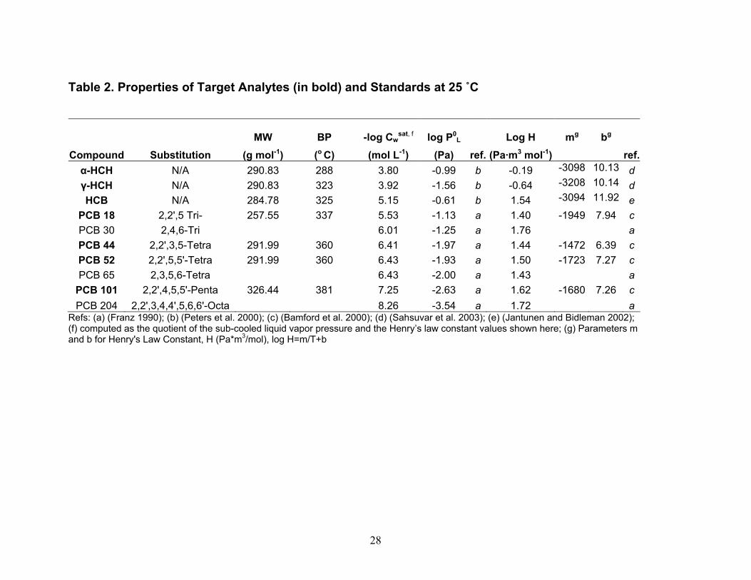
28

Table 2. Properties of Target Analytes (in bold) and Standards at 25 ˚C

MW

BP -log Cwsat, f log P0

L Log H

mg

bg

Compound Substitution (g mol-1) (o C) (mol L-1) (Pa) ref. (Pa·m3 mol-1) ref.α-HCH N/A 290.83 288 3.80 -0.99 b -0.19 -3098 10.13 dγ-HCH N/A 290.83 323 3.92 -1.56 b -0.64 -3208 10.14 dHCB N/A 284.78 325 5.15 -0.61 b 1.54 -3094 11.92 e

PCB 18 2,2',5 Tri- 257.55 337 5.53 -1.13 a 1.40 -1949 7.94 c PCB 30 2,4,6-Tri 6.01 -1.25 a 1.76 aPCB 44 2,2',3,5-Tetra 291.99 360 6.41 -1.97 a 1.44 -1472 6.39 c PCB 52 2,2',5,5'-Tetra 291.99 360 6.43 -1.93 a 1.50 -1723 7.27 c PCB 65 2,3,5,6-Tetra 6.43 -2.00 a 1.43 a

PCB 101 2,2',4,5,5'-Penta 326.44 381 7.25 -2.63 a 1.62 -1680 7.26 c PCB 204 2,2',3,4,4',5,6,6'-Octa 8.26 -3.54 a 1.72 a

Refs: (a) (Franz 1990); (b) (Peters et al. 2000); (c) (Bamford et al. 2000); (d) (Sahsuvar et al. 2003); (e) (Jantunen and Bidleman 2002); (f) computed as the quotient of the sub-cooled liquid vapor pressure and the Henry’s law constant values shown here; (g) Parameters m and b for Henry's Law Constant, H (Pa*m3/mol), log H=m/T+b

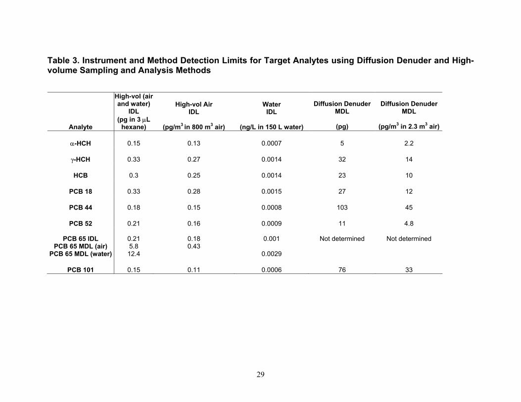
29

Table 3. Instrument and Method Detection Limits for Target Analytes using Diffusion Denuder and High-volume Sampling and Analysis Methods

Analyte

High-vol (air and water)

IDL (pg in 3 µL

hexane)

High-vol Air IDL

(pg/m3 in 800 m3 air)

Water IDL

(ng/L in 150 L water)

Diffusion Denuder

MDL

(pg)

Diffusion Denuder

MDL

(pg/m3 in 2.3 m3 air)

α-HCH 0.15 0.13 0.0007 5 2.2

γ-HCH 0.33 0.27 0.0014 32 14

HCB 0.3 0.25 0.0014 23 10

PCB 18 0.33 0.28 0.0015 27 12

PCB 44 0.18 0.15 0.0008 103 45

PCB 52 0.21 0.16 0.0009 11 4.8

PCB 65 IDL PCB 65 MDL (air)

PCB 65 MDL (water)

0.21 5.8 12.4

0.18 0.43

0.001

0.0029

Not determined

Not determined

PCB 101 0.15 0.11 0.0006 76 33

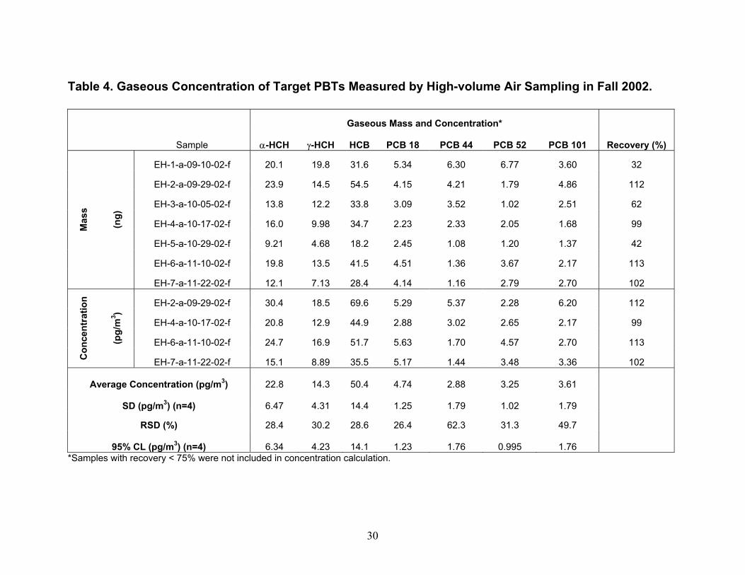
30

Table 4. Gaseous Concentration of Target PBTs Measured by High-volume Air Sampling in Fall 2002.

Gaseous Mass and Concentration*

Sample α-HCH γ-HCH HCB PCB 18 PCB 44 PCB 52 PCB 101 Recovery (%)

EH-1-a-09-10-02-f 20.1 19.8 31.6 5.34 6.30 6.77 3.60 32

EH-2-a-09-29-02-f 23.9 14.5 54.5 4.15 4.21 1.79 4.86 112

EH-3-a-10-05-02-f 13.8 12.2 33.8 3.09 3.52 1.02 2.51 62

EH-4-a-10-17-02-f 16.0 9.98 34.7 2.23 2.33 2.05 1.68 99

EH-5-a-10-29-02-f 9.21 4.68 18.2 2.45 1.08 1.20 1.37 42

EH-6-a-11-10-02-f 19.8 13.5 41.5 4.51 1.36 3.67 2.17 113

Mas

s

(ng)

EH-7-a-11-22-02-f 12.1 7.13 28.4 4.14 1.16 2.79 2.70 102

EH-2-a-09-29-02-f 30.4 18.5 69.6 5.29 5.37 2.28 6.20 112

EH-4-a-10-17-02-f 20.8 12.9 44.9 2.88 3.02 2.65 2.17 99

EH-6-a-11-10-02-f 24.7 16.9 51.7 5.63 1.70 4.57 2.70 113

Con

cent

ratio

n

(pg/

m3 )

EH-7-a-11-22-02-f 15.1 8.89 35.5 5.17 1.44 3.48 3.36 102

Average Concentration (pg/m3) 22.8 14.3 50.4 4.74 2.88 3.25 3.61

SD (pg/m3) (n=4) 6.47 4.31 14.4 1.25 1.79 1.02 1.79

RSD (%) 28.4 30.2 28.6 26.4 62.3 31.3 49.7

95% CL (pg/m3) (n=4) 6.34 4.23 14.1 1.23 1.76 0.995 1.76 *Samples with recovery < 75% were not included in concentration calculation.

31

Table 5. Gaseous Concentration of Target PBTs Measured by High-volume Air Sampling in Spring 2003.

Gaseous Mass and Concentration*

Sample α-HCH γ-HCH HCB PCB 18 PCB 44 PCB 52 PCB 101 Recovery (%)

SU-1-a-04-25-03-f 15.4 32.4 14.2 6.07 5.02 4.18 3.05 101

SU-2-a-04-25-03-f 10.8 11.7 9.29 7.68 3.95 8.63 4.95 92

EH-3-a-04-26-03-f 9.40 29.8 27.4 3.00 6.23 3.66 7.59 101

EH-4-a-04-26-03-f 9.98 12.5 31.7 4.08 2.99 1.31 4.83 108

Mas

s

(ng)

EH-5-a-05-22-03-f 16.1 22.1 20.6 12.3 7.68 3.31 6.06 61

SU-1-a-04-25-03-f 31.2 65.9 28.8 12.3 10.2 8.50 6.19 101

SU-2-a-04-25-03-f 20.0 21.6 17.2 14.2 7.29 15.9 9.13 92

EH-3-a-04-26-03-f 9.50 30.1 27.7 3.03 6.30 3.70 7.67 101

Con

cent

ratio

n

(pg

/m3 )

EH-4-a-04-26-03-f 12.6 15.8 40.2 5.16 3.78 1.66 6.12 108

Average Concentration (pg/m3) 18.4 33.4 28.5 8.67 6.89 7.45 7.28

SD (pg/m3) (n=4) 9.65 22.4 9.44 5.41 2.65 6.34 1.43

RSD (%) 52.6 67.3 33.2 62.3 38.4 85.1 19.6

95% CL (pg/m3) (n=4) 9.17 21.3 8.97 5.14 2.51 6.02 1.36 *Samples with recovery < 75% were not included in concentration calculation.

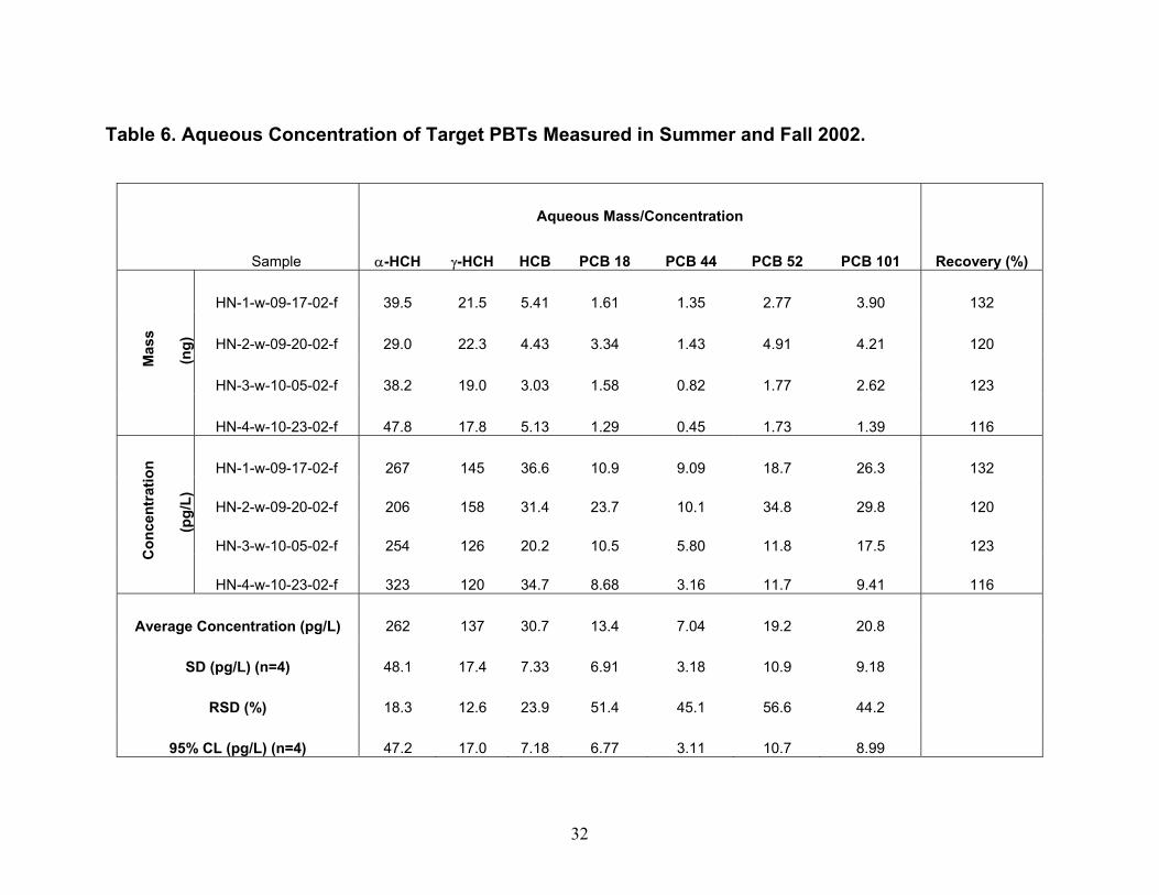
32

Table 6. Aqueous Concentration of Target PBTs Measured in Summer and Fall 2002.

Aqueous Mass/Concentration

Sample α-HCH γ-HCH HCB PCB 18 PCB 44 PCB 52 PCB 101 Recovery (%)

HN-1-w-09-17-02-f 39.5 21.5 5.41 1.61 1.35 2.77 3.90 132

HN-2-w-09-20-02-f 29.0 22.3 4.43 3.34 1.43 4.91 4.21 120

HN-3-w-10-05-02-f 38.2 19.0 3.03 1.58 0.82 1.77 2.62 123

Mas

s

(ng)

HN-4-w-10-23-02-f 47.8 17.8 5.13 1.29 0.45 1.73 1.39 116

HN-1-w-09-17-02-f 267 145 36.6 10.9 9.09 18.7 26.3 132

HN-2-w-09-20-02-f 206 158 31.4 23.7 10.1 34.8 29.8 120

HN-3-w-10-05-02-f 254 126 20.2 10.5 5.80 11.8 17.5 123

Con

cent

ratio

n

(pg/

L)

HN-4-w-10-23-02-f 323 120 34.7 8.68 3.16 11.7 9.41 116

Average Concentration (pg/L) 262 137 30.7 13.4 7.04 19.2 20.8

SD (pg/L) (n=4) 48.1 17.4 7.33 6.91 3.18 10.9 9.18

RSD (%) 18.3 12.6 23.9 51.4 45.1 56.6 44.2

95% CL (pg/L) (n=4) 47.2 17.0 7.18 6.77 3.11 10.7 8.99

33

Table 7. Aqueous Concentration of Target PBTs Measured in Spring 2003.

Aqueous Mass/Concentration

Sample α-HCH γ-HCH HCB PCB 18 PCB 44 PCB 52 PCB 101 Recovery (%)

SU-1-w-04-25-03-f 96.6 27.1 3.70 0.935 0.759 2.18 1.17 102

EH-2-w-04-26-03-f 104 29.3 3.31 1.48 0.729 1.63 0.688 107

EH-3-w-04-26-03-f 102 27.7 3.82 0.842 0.795 1.55 0.812 116

Mas

s

(ng)

EH-4-w-05-25-03-f 25.5 10.2 2.45 0.749 0.604 1.38 1.70 112

SU-1-w-04-25-03-f 421 118 16.1 4.08 3.31 9.51 5.12 102

EH-2-w-04-26-03-f 450 127 14.3 6.42 3.16 7.05 2.98 107

EH-3-w-04-26-03-f 480 131 18.0 3.98 3.75 7.30 3.83 116

Con

cent

ratio

n

(pg

/L)

EH-4-w-05-25-03-f 159 63.7 15.3 4.68 3.78 8.64 10.6 112

Average Concentration (pg/L) 378 110 16.0 4.79 3.50 8.12 5.64

SD (pg/L) (n=4) 148 31.3 1.56 1.13 0.31 1.16 3.44

RSD (%) 39.1 28.4 9.79 23.6 8.9 14.2 61.0

95% CL (pg/L) (n=4) 145 30.6 1.53 1.11 0.307 1.13 3.37

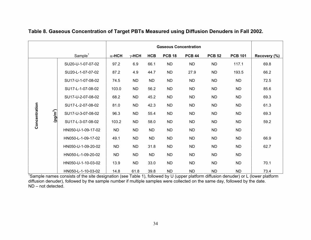
34

Table 8. Gaseous Concentration of Target PBTs Measured using Diffusion Denuders in Fall 2002.

Gaseous Concentration

Sample1 α-HCH γ-HCH HCB PCB 18 PCB 44 PCB 52 PCB 101 Recovery (%)

SU20-U-1-07-07-02 97.2 6.9 66.1 ND ND ND 117.1 69.8

SU20-L-1-07-07-02 87.2 4.9 44.7 ND 27.9 ND 193.5 66.2

SU17-U-1-07-08-02 74.5 ND ND ND ND ND ND 72.5

SU17-L-1-07-08-02 103.0 ND 56.2 ND ND ND ND 85.6

SU17-U-2-07-08-02 68.2 ND 45.2 ND ND ND ND 69.3

SU17-L-2-07-08-02 81.0 ND 42.3 ND ND ND ND 61.3

SU17-U-3-07-08-02 96.3 ND 55.4 ND ND ND ND 69.3

SU17-L-3-07-08-02 103.2 ND 58.0 ND ND ND ND 59.2

HN050-U-1-09-17-02 ND ND ND ND ND ND ND

HN050-L-1-09-17-02 49.1 ND ND ND ND ND ND 66.9

HN050-U-1-09-20-02 ND ND 31.8 ND ND ND ND 62.7

HN050-L-1-09-20-02 ND ND ND ND ND ND ND

HN050-U-1-10-03-02 13.9 ND 33.0 ND ND ND ND 70.1

Con

cent

ratio

n

(pg/

m3 )

HN050-L-1-10-03-02 14.8 61.8 39.8 ND ND ND ND 73.4 1Sample names consists of the site designation (see Table 1), followed by U (upper platform diffusion denuder) or L (lower platform diffusion denuder), followed by the sample number if multiple samples were collected on the same day, followed by the date. ND – not detected.

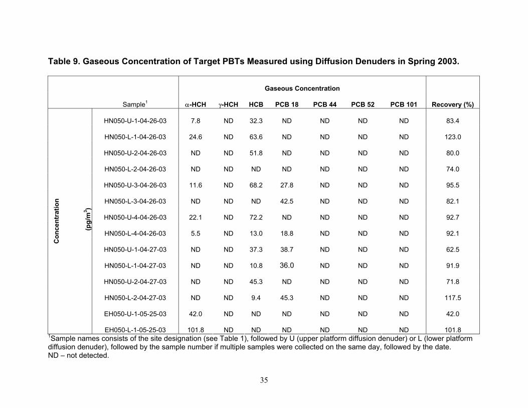
35

Table 9. Gaseous Concentration of Target PBTs Measured using Diffusion Denuders in Spring 2003.

Gaseous Concentration

Sample1 α-HCH γ-HCH HCB PCB 18 PCB 44 PCB 52 PCB 101 Recovery (%)

HN050-U-1-04-26-03 7.8 ND 32.3 ND ND ND ND 83.4

HN050-L-1-04-26-03 24.6 ND 63.6 ND ND ND ND 123.0

HN050-U-2-04-26-03 ND ND 51.8 ND ND ND ND 80.0

HN050-L-2-04-26-03 ND ND ND ND ND ND ND 74.0

HN050-U-3-04-26-03 11.6 ND 68.2 27.8 ND ND ND 95.5

HN050-L-3-04-26-03 ND ND ND 42.5 ND ND ND 82.1

HN050-U-4-04-26-03 22.1 ND 72.2 ND ND ND ND 92.7

HN050-L-4-04-26-03 5.5 ND 13.0 18.8 ND ND ND 92.1

HN050-U-1-04-27-03 ND ND 37.3 38.7 ND ND ND 62.5

HN050-L-1-04-27-03 ND ND 10.8 36.0 ND ND ND 91.9

HN050-U-2-04-27-03 ND ND 45.3 ND ND ND ND 71.8

HN050-L-2-04-27-03 ND ND 9.4 45.3 ND ND ND 117.5

EH050-U-1-05-25-03 42.0 ND ND ND ND ND ND 42.0

Con

cent

ratio

n

(pg

/m3 )

EH050-L-1-05-25-03 101.8 ND ND ND ND ND ND 101.8 1Sample names consists of the site designation (see Table 1), followed by U (upper platform diffusion denuder) or L (lower platform diffusion denuder), followed by the sample number if multiple samples were collected on the same day, followed by the date. ND – not detected.

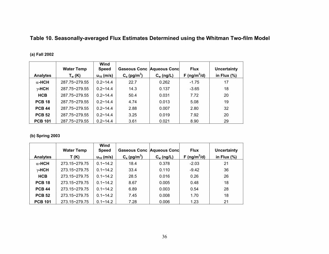
36

Table 10. Seasonally-averaged Flux Estimates Determined using the Whitman Two-film Model

(a) Fall 2002

Water Temp Wind

Speed Gaseous Conc Aqueous Conc Flux Uncertainty Analytes Tw (K) u10 (m/s) Ca (pg/m3) Cw (ng/L) F (ng/m2/d) in Flux (%)

α-HCH 287.75~279.55 0.2~14.4 22.7 0.262 -1.75 17 γ-HCH 287.75~279.55 0.2~14.4 14.3 0.137 -3.65 18 HCB 287.75~279.55 0.2~14.4 50.4 0.031 7.72 20

PCB 18 287.75~279.55 0.2~14.4 4.74 0.013 5.08 19 PCB 44 287.75~279.55 0.2~14.4 2.88 0.007 2.80 32 PCB 52 287.75~279.55 0.2~14.4 3.25 0.019 7.92 20 PCB 101 287.75~279.55 0.2~14.4 3.61 0.021 8.90 29

(b) Spring 2003

Water Temp Wind

Speed Gaseous Conc Aqueous Conc Flux Uncertainty Analytes T (K) u10 (m/s) Ca (pg/m3) Cw (ng/L) F (ng/m2/d) in Flux (%)

α-HCH 273.15~279.75 0.1~14.2 18.4 0.378 -2.03 21 γ-HCH 273.15~279.75 0.1~14.2 33.4 0.110 -9.42 36 HCB 273.15~279.75 0.1~14.2 28.5 0.016 0.26 26

PCB 18 273.15~279.75 0.1~14.2 8.67 0.005 0.48 18 PCB 44 273.15~279.75 0.1~14.2 6.89 0.003 0.54 28 PCB 52 273.15~279.75 0.1~14.2 7.45 0.008 1.70 18 PCB 101 273.15~279.75 0.1~14.2 7.28 0.006 1.23 21

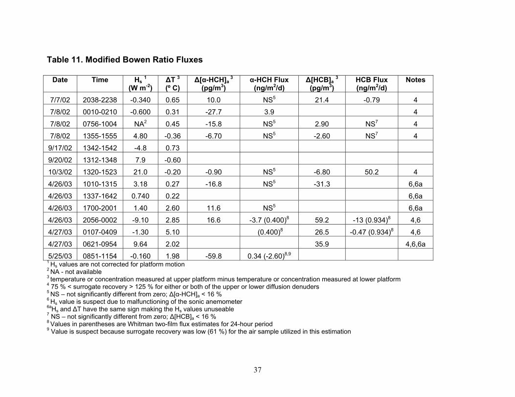
37

Table 11. Modified Bowen Ratio Fluxes

Date Time Hs 1

(W m-2) ∆T 3

(º C) ∆[α-HCH]a

3 (pg/m3)

α-HCH Flux (ng/m2/d)

∆[HCB]a 3

(pg/m3) HCB Flux (ng/m2/d)

Notes

7/7/02 2038-2238 -0.340 0.65 10.0 NS5 21.4 -0.79 4

7/8/02 0010-0210 -0.600 0.31 -27.7 3.9 4

7/8/02 0756-1004 NA2 0.45 -15.8 NS5 2.90 NS7 4

7/8/02 1355-1555 4.80 -0.36 -6.70 NS5 -2.60 NS7 4

9/17/02 1342-1542 -4.8 0.73

9/20/02 1312-1348 7.9 -0.60

10/3/02 1320-1523 21.0 -0.20 -0.90 NS5 -6.80 50.2 4

4/26/03 1010-1315 3.18 0.27 -16.8 NS5 -31.3 6,6a

4/26/03 1337-1642 0.740 0.22 6,6a

4/26/03 1700-2001 1.40 2.60 11.6 NS5 6,6a

4/26/03 2056-0002 -9.10 2.85 16.6 -3.7 (0.400)8 59.2 -13 (0.934)8 4,6

4/27/03 0107-0409 -1.30 5.10 (0.400)8 26.5 -0.47 (0.934)8 4,6

4/27/03 0621-0954 9.64 2.02 35.9 4,6,6a

5/25/03 0851-1154 -0.160 1.98 -59.8 0.34 (-2.60)8,9 1 Hs values are not corrected for platform motion 2 NA - not available 3 temperature or concentration measured at upper platform minus temperature or concentration measured at lower platform 4 75 % < surrogate recovery > 125 % for either or both of the upper or lower diffusion denuders 5 NS – not significantly different from zero; ∆[α-HCH]a < 16 % 6 Hs value is suspect due to malfunctioning of the sonic anemometer 6aHs and ∆T have the same sign making the Hs values unuseable 7 NS – not significantly different from zero; ∆[HCB]a < 16 % 8 Values in parentheses are Whitman two-film flux estimates for 24-hour period 9 Value is suspect because surrogate recovery was low (61 %) for the air sample utilized in this estimation

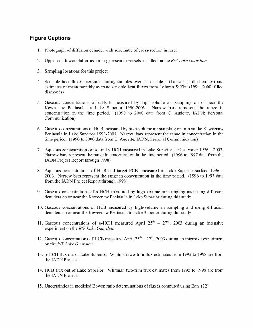
Figure Captions

1. Photograph of diffusion denuder with schematic of cross-section in inset 2. Upper and lower platforms for large research vessels installed on the R/V Lake Guardian

3. Sampling locations for this project 4. Sensible heat fluxes measured during samples events in Table 1 (Table 11; filled circles) and

estimates of mean monthly average sensible heat fluxes from Lofgren & Zhu (1999, 2000; filled diamonds)

5. Gaseous concentrations of α-HCH measured by high-volume air sampling on or near the

Keweenaw Peninsula in Lake Superior 1990-2003. Narrow bars represent the range in concentration in the time period. (1990 to 2000 data from C. Audette, IADN; Personal Communication)

6. Gaseous concentrations of HCB measured by high-volume air sampling on or near the Keweenaw

Peninsula in Lake Superior 1990-2003. Narrow bars represent the range in concentration in the time period. (1990 to 2000 data from C. Audette, IADN; Personal Communication)

7. Aqueous concentrations of α- and γ-HCH measured in Lake Superior surface water 1996 – 2003.

Narrow bars represent the range in concentration in the time period. (1996 to 1997 data from the IADN Project Report through 1998)

8. Aqueous concentrations of HCB and target PCBs measured in Lake Superior surface 1996 –

2003. Narrow bars represent the range in concentration in the time period. (1996 to 1997 data from the IADN Project Report through 1998)

9. Gaseous concentrations of α-HCH measured by high-volume air sampling and using diffusion

denuders on or near the Keweenaw Peninsula in Lake Superior during this study

10. Gaseous concentrations of HCB measured by high-volume air sampling and using diffusion denuders on or near the Keweenaw Peninsula in Lake Superior during this study

11. Gaseous concentrations of α-HCH measured April 25th – 27th, 2003 during an intensive

experiment on the R/V Lake Guardian

12. Gaseous concentrations of HCB measured April 25th – 27th, 2003 during an intensive experiment on the R/V Lake Guardian

13. α-HCH flux out of Lake Superior. Whitman two-film flux estimates from 1995 to 1998 are from

the IADN Project.

14. HCB flux out of Lake Superior. Whitman two-film flux estimates from 1995 to 1998 are from the IADN Project.

15. Uncertainties in modified Bowen ratio determinations of fluxes computed using Eqn. (22)

39

Diffusion Denuder

Figure 1

40

Figure 2

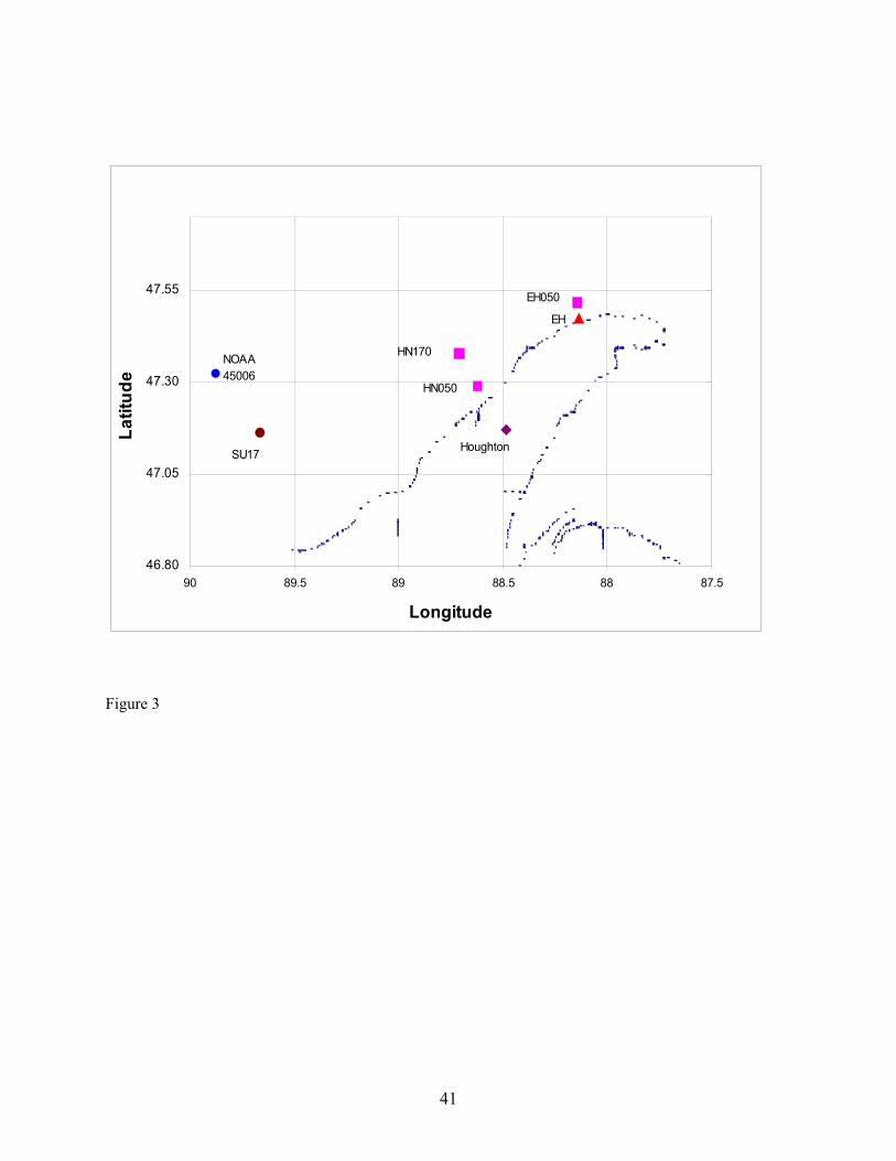
41

Figure 3

46.80

47.05

47.30

47.55

87.58888.58989.590

Longitude

Latit

ude

EH

HN050

HN170NOAA 45006

HoughtonSU17

EH050

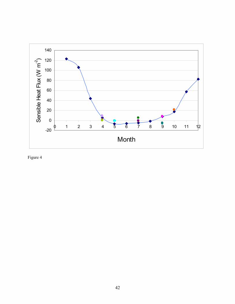
42

Figure 4

-20

0

20

40

60

80

100

120

140

0 1 2 3 4 5 6 7 8 9 10 11 12

Month

Sens

ible

Hea

t Flu

x (W

m-2

)

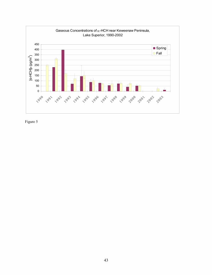
43

Figure 5

Gaseous Concentrations of α-HCH near Keweenaw Peninsula, Lake Superior, 1990-2002

0

50

100

150

200

250

300

350

400

450

1990

1991

1992

1993

1994

1995

1996

1997

1998

1999

2000

2001

2002

2003

[α-H

CH

]a (p

g/m

3 )

SpringFall

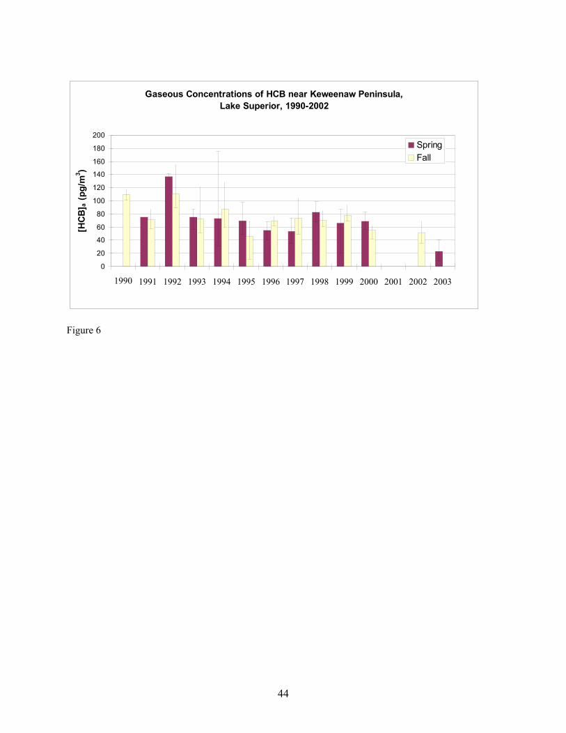
44

Figure 6

Gaseous Concentrations of HCB near Keweenaw Peninsula, Lake Superior, 1990-2002

0

20

40

60

80

100

120

140

160

180

200

1990 1991 1992 1993 1994 1995 1996 1997 1998 1999 2000 2001 2002 2003

[HC

B] a

(pg/

m3 )

SpringFall

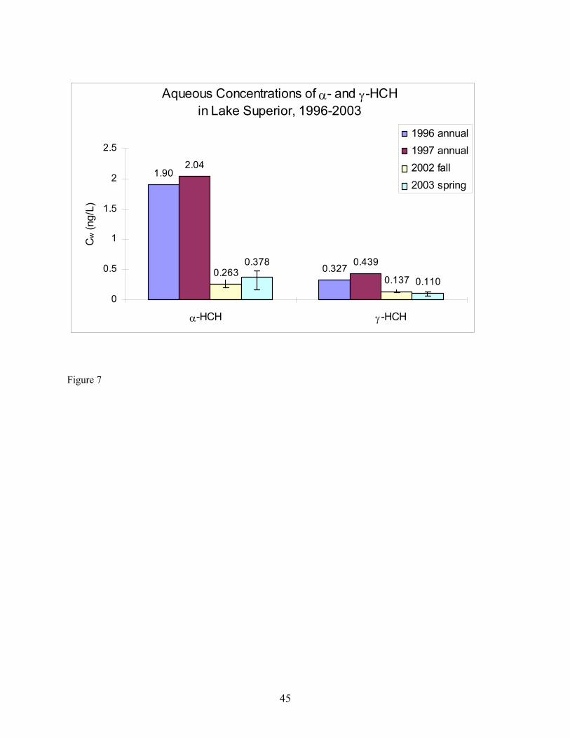
45

Figure 7

Aqueous Concentrations of α- and γ-HCH in Lake Superior, 1996-2003

1.90

0.327

2.04

0.4390.263

0.137

0.378

0.110

0

0.5

1

1.5

2

2.5

Cw (n

g/L)

1996 annual1997 annual2002 fall2003 spring

γ -HCHα-HCH

46

Figure 8

Aqueous Concentrations of HCB and PCBs in Lake Superior, 1996-2003

0

0.005

0.01

0.015

0.02

0.025

0.03

0.035

0.04

Cw (n

g/L)

1996 annual1997 annual2002 fall2003 spring

PCB 101HCB PCB 18 PCB 44 PCB 52

47

0

20

40

60

80

100

120

7/7/20

02

7/8/20

02

9/17/2

002

9/29/2

002

10/17

/2002

11/22

/2002

4/25/2

003

4/26/2

003

4/26/2

003

4/26/2

003

4/27/2

003

5/22/2

003

[α-H

CH

] a (p

g m

-3)

upper denuder

lower denuder

High-vol

Figure 9

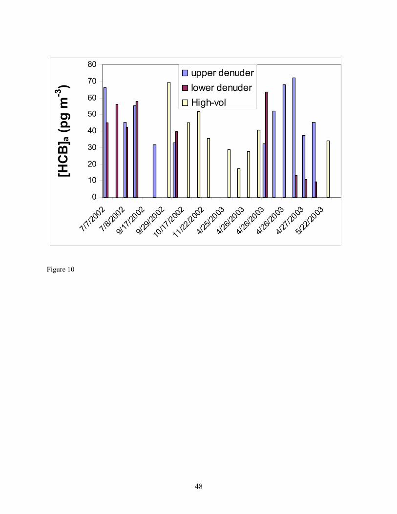
48

0

10

20

30

40

50

60

70

80

7/7/20

02

7/8/20

02

9/17/2

002

9/29/2

002

10/17

/2002

11/22

/2002

4/25/2

003

4/26/2

003

4/26/2

003

4/26/2

003

4/27/2

003

5/22/2

003

[HC

B] a

(pg

m-3

)upper denuderlower denuderHigh-vol

Figure 10

49

31.2

9.5

20

12.6

7.8

11.6

22.124.6

5.5

0

5

10

15

20

25

30

35

0.0 13.7 17.1 20.5 24.4

Initiation of Sampling after T0 (hrs)

[α-H

CH

] a (p

g m

-3)

High-vol 1, 4.8 m AW

High-vol 2, 4.8 m AW

upper denuder, 8.5 m AW

lower denuder, 1 m AW

Figure 11

50

65.9

30.1

21.615.8

32.3

51.8

68.272.2

37.3

45.3

63.6

13 10.8 9.4

0

10

20

30

40

50

60

70

0 13.7 17.1 20.5 24.4 27.6 32.9

Initiation of Sampling after T0 (hrs)

[HC

B] a

(pg

m-3

)

High-vol 1, 4.8 m AW

High-vol 2, 4.8 m AW

upper denuder 8.5 mAW

lower denuder 1 m AW

Figure 12

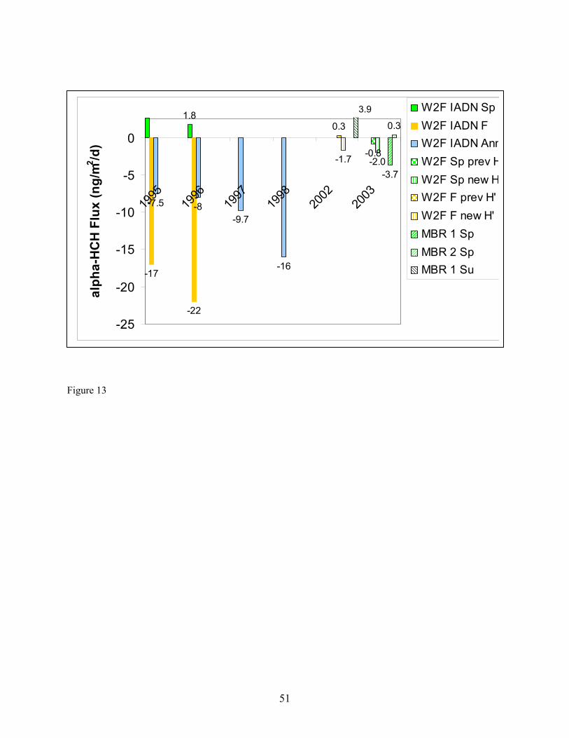
51

Figure 13

1.8

-17

-22

-7.5 -8-9.7

-16

-0.8-2.0

0.3

-1.7-3.7

0.3

-25

-20

-15

-10

-5

0

1995

1996

1997

1998

2002

2003

alph

a-H

CH

Flu

x (n

g/m

2 /d)

W2F IADN SpW2F IADN FW2F IADN AnnW2F Sp prev HW2F Sp new HW2F F prev H'W2F F new H'MBR 1 SpMBR 2 SpMBR 1 Su

3.9

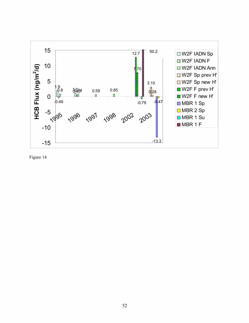
52

1.9 1.1

-0.49

0.450.8 0.74 0.59 0.85

3.10

0.28

12.7

7.70

-13.3

-0.47-0.79

-15

-10

-5

0

5

10

15

19951996

19971998

20022003H

CB

Flu

x (n

g/m

2 /d)

W2F IADN SpW2F IADN FW2F IADN AnnW2F Sp prev H'W2F Sp new H'W2F F prev H'W2F F new H'MBR 1 SpMBR 2 SpMBR 1 SuMBR 1 F

Figure 14

50.2

53

Figure 15

Predicted Uncertainty in Measured Fluxes

-1.0

0.0

1.0

2.0

3.0

4.0

0.1 0.5 1 0.1 0.5 1 0.1 0.5 1

F/[PBT]avg (cm/s)

log(

Unc

erta

inty

, %)

u* = 10 cm/su* = 30 cm/su* = 100 cm/s

UNSTABLE NEUTRAL STABLE