San Jose State UniversitySJSU ScholarWorks

Master's Theses Master's Theses and Graduate Research

Summer 2018

Micrometeorological Observations of Fire-Atmosphere Interactions and Fire Behavior on aSimple SlopeJonathan Marc ContezacSan Jose State University

Follow this and additional works at: https://scholarworks.sjsu.edu/etd_theses

This Thesis is brought to you for free and open access by the Master's Theses and Graduate Research at SJSU ScholarWorks. It has been accepted forinclusion in Master's Theses by an authorized administrator of SJSU ScholarWorks. For more information, please contact scholarworks@sjsu.edu.

Recommended CitationContezac, Jonathan Marc, "Micrometeorological Observations of Fire-Atmosphere Interactions and Fire Behavior on a Simple Slope"(2018). Master's Theses. 4934.DOI: https://doi.org/10.31979/etd.d7nc-77e4https://scholarworks.sjsu.edu/etd_theses/4934

MICROMETEOROLOGICAL OBSERVATIONS OF FIRE-ATMOSPHERE INTERACTIONS AND FIRE BEHAVIOR ON A SIMPLE SLOPE

A Thesis

Presented to

The Faculty of the Department of Meteorology and Climate Science

San José State University

In Partial Fulfillment

of the Requirements for the Degree

Master of Science

by

Jonathan M. Contezac

August 2018

© 2018

Jonathan M. Contezac

ALL RIGHTS RESERVED

The Designated Thesis Committee Approves the Thesis Titled

MICROMETEOROLOGICAL OBSERVATIONS OF FIRE-ATMOSPHERE INTERACTIONS AND FIRE BEHAVIOR ON A SIMPLE SLOPE

by

Jonathan M. Contezac

APPROVED FOR THE DEPARTMENT OF METEOROLOGY AND

CLIMATE SCIENCE

SAN JOSÉ STATE UNIVERSITY

August 2018

Dr. Craig B. Clements Department of Meteorology and Climate Science

Dr. Sen Chiao Department of Meteorology and Climate Science

Dr. Neil Lareau Department of Meteorology and Climate Science

ABSTRACT

by Jonathan M. Contezac

An experiment was designed to capture micrometeorological observations

during a fire spread on a simple slope. Three towers equipped with a variety of

instrumentation, an array of fire-sensing packages, and a Doppler lidar was

deployed to measure various aspects of the fire. Pressure and temperature

perturbations were analyzed for each of the grid packages to determine if the fire

intensity could be observed in the covariance of the two variables. While two of

the packages measured a covariance less than -15 °C hPa, there was no clear

trend across the grid. The fire front passage at each of the three towers on the

slope yielded extreme swings in observed turbulent kinetic energy and sensible

heat flux. Vertical velocity turbulence spectra showed that the high-intensity fire

front passage at the bottom tower was 2 to 3 orders of magnitude larger than the

low-intensity fire front passages at the top two towers. Opposing wind regimes on

the slope caused a unique L-shaped pattern to form in the fire front. A vorticity

estimation from the sonic anemometers showed that vorticity reached a

maximum just as a fire whirl formed in the bend of the L-shaped fire front, leading

to a rapid increase in fire spread.

v

ACKNOWLEDGEMENTS

I would like to thank Dr. Craig Clements for all the opportunities he provided

me during my time at San Jose State University. The skills I learned while

tinkering and building in the Fire Lab have aided me greater than any class has.

And I wouldn’t be where I am without his knowledge, wisdom, and patience.

I’d also like to thank Drs. Sen Chiao and Neil Lareau for serving on my thesis

committee at the eleventh hour. This would not be possible without their support.

Thanks also must go to Dianne Hall and Braniff Davis for providing a few of

the GIS maps.

Additionally, the Fort Hunter Liggett Fire Department is thanked for their help

in logistics, executing, and managing all fire operations for our project.

Lastly, I wanted to thank all the faculty, staff, and students in the meteorology

department, as well as my family and friends. It was a lot of hard work and effort

to get through the program and I probably would not have succeeded without

everyone’s support.

Funding of this research was provided by the National Institute of

Standards Fire Research Grants Program Award #60NANB11D189.

vi

TABLE OF CONTENTS

List of Tables……………………………………………………………… vii

List of Figures…………………………………………………………….. viii

Chapter 1: Introduction…………………………………………………... 1

Chapter 2: Experimental Design………………………………………… 9 2.1 Site Selection and Characteristics……………………………… 9 2.2 Field Experimental Design………………………………………. 12 2.3 Micrometeorological Measurements………………………….... 13 2.4 Ambient Meteorological Measurements.………………………. 18 2.5 Synoptic Overview……………………………………………….. 21

Chapter 3: Temperature Pressure Perturbations……………………… 22 3.1 Introduction……………………………………………………….. 22 3.2 Methods and Data Processing………………………………….. 24 3.3 Results and Discussion………………………………………….. 27 3.4 Conclusion………………………………………………………… 35

Chapter 4: Micrometeorology……………………………………………. 36 4.1 Introduction……………………………………………………….. 36 4.2 Data Processing………………………………………………….. 38 4.3 Fire Front Passage………………………………………………. 40 4.4 Summary………………………………………………………….. 56

Chapter 5: Vorticity Estimation and Fire Whirls……………………….. 57 5.1 Introduction……………………………………………………….. 57 5.2 Data Processing………………………………………………….. 58 5.3 Description of Event……………………………………………… 59 5.4 Results…………………………………………………………….. 61 5.5 Summary and Conclusion……………………………………….. 68

Chapter 6: Summary and Conclusion………………………………….. 68

References………………………………………………………………… 71

vii

LIST OF TABLES

Table 1. Uniform sensors per tower………………………………….. 15

Table 2. FSP IDs and offsets made to each dataset……………….. 25

viii

LIST OF FIGURES

Figure 1. County map of California showing the names and areas of the 10 largest wildfires in California up to July 2013………………………………………………………….

3

Figure 2. Percent of area burned for a given slope angle for each of California’s largest wildfires…………………………….

4

Figure 3. Regional road map of west central California…………...

9

Figure 4. Map of experimentation site……………………………….

10

Figure 5. 3D satellite image of the burn plot generated from elevation data. Elevation contours are plotted across the slope…………………………………………………….

10

Figure 6. Detailed map of the burn area…………………………….

11

Figure 7. Photo of the burn area, pre-burn………………………….

14

Figure 8. Aerial imagery of the (a) ignition line and fire front passage at the (b) bottom, (c) middle, and (d) top towers………………………………………………………..

18

Figure 9. Photo of Doppler SODAR (left) and CSU-MAPS tower (right)…………………………………………………………

19

Figure 10. Photo of Doppler LIDAR…………………………………...

20

Figure 11. The 12Z 500 hPa analysis from 20 June 2012………….

21

Figure 12. The 12Z 850 hPa analysis from 20 June 2012………….

22

Figure 13. The 12Z surface analysis from 20 June 2012…………..

23

Figure 14. Temperature time series from each of the FSPs in the grid…………………………………………………………...

28

Figure 15. Estimated rate of spread through sensor grid…………..

29

Figure 16. An aerial photo of the fire………………………………….

30

ix

Figure 17. Temperature and pressure time series with covariance plots for the duration of the fire front passage for each FSP (a-v)…………………………………………………….

31,32,33

Figure 18. Slope-valley wind coordinate system…………………….

38

Figure 19. Time series of u, v, and w velocities, as well as sonic temperature for the bottom tower (blue), middle tower (red), and top tower (magenta)……………………………

41

Figure 20. Five minute averaged two meter wind speed at RAWS located in the valley (red) and ridge (black)……………..

42

Figure 21. Radiative heat flux measured at the bottom (blue) and middle (red) towers…………………………………………

43

Figure 22. (a) shows the TKE and Hs observed at the bottom tower during FFP. (b) shows the velocity variances at the bottom tower during the same time frame…………..

44

Figure 23. (a) is a RHI scan performed by the Doppler lidar during the FFP at the bottom tower. (b) is a corresponding aerial photograph…………………………………………..

46

Figure 24. (a) shows the TKE and Hs observed at the middle tower during FFP. (b) shows the velocity variances at the middle tower during the same time frame…………..

47

Figure 25. (a) is a RHI scan from the Doppler lidar taken during FFP at the middle tower. (b) is a corresponding aerial photograph…………………………………………………..

49

Figure 26. (a) shows the TKE and Hs observed at the top tower during FFP. (b) shows the velocity variances at the top tower during the same time frame………………………..

50

Figure 27. Four photos taken in 1-minute intervals depicting the downslope wind dispersing the smoke down the slope..

51

Figure 28. Perturbation time series of sonic temperature (a) and vertical velocity (b) from the top tower during a downslope wind…………………………………………….

52

x

Figure 29. Momentum flux time series for (a) horizontal winds, (b) slope winds, and (c) cross-slope winds……………...

53

Figure 30. Normalized power spectra during fire front passage at

each tower for (a) u, (b) v, and (c) w wind velocities, as well as (d) sonic temperature. The bottom tower is in blue, middle in red, top in magenta………………………

55

Figure 31. 10-minute averaged sodar wind profile observed near the valley center…………………………………………….

59

Figure 32. A series of photos depicting an L-shaped fireline, a fire whirl, and the resulting rapid increase in the rate of spread……………………………………………………….

60

Figure 33. A map of 1-minute interval fireline locations georeferenced from aerial photography………………….

61

Figure 34. Lidar RHI scan taken during the northeasterly wind……

62

Figure 35. Time series of estimated horizontal vorticity during the time of increased fire spread……………………………...

63

Figure 36. A lidar PPI scan of alternating inbound and outbound winds over the valley……………………………………….

64

Figure 37. A series of lidar PPI scans depicting a velocity couplet forming near the ridge and propagating downslope and across the valley……………………………………………

65

Figure 38. A photo of a whirl lifting ash into the air in the wake of the fire………………………………………………………..

66

1

Chapter 1 - Introduction

The interactions between wildland fires and the atmosphere are complex and

dynamic (Jenkins et al., 2001; Potter 2014a; 2014b). On the large scale, long-

term global oscillations have been shown to have a strong correlation with high

fire activity (Kitzberger et al. 2007). Although, debate does remain as to the link

between changing climate and increased fire activity (Westering et al. 2006).

Fluctuations in fire activity have a direct impact on local ecosystems and

economies, as management of wildfires still remains imperfect (Bowman et al.

2009). Despite this flaw, our knowledge of critical weather patterns leading to

increased fire activity has greatly improved (Werth 2011).

Over the past century, research in the area of fire meteorology has identified

synoptic scale patterns associated with increased fire activity. It was Beals

(1914) who first identified the pressure, temperature, and wind patterns

associated with large fires. Later, Schroeder et al. (1964) produced a complete

analysis of fire weather patterns over the continental United States. It was shown

that, for states bordering the Pacific Ocean, synoptic patterns producing offshore

flow, or foehn winds, favored wildfire development (Werth 2011).

Schroeder et al. (1964) proposed that offshore flow in California is produced

by an upper level northwest to southeast pressure gradient. Typically, this setup

occurs when sea level pressure is elevated in the Great Basin region (Conil and

Hall 2006; Raphael 2003). This area of high pressure forces the thermally

2

induced low within the Central Valley offshore, creating a strong pressure

gradient over California. This pressure gradient is the source of the föhn winds.

Several additional studies have indicated links between synoptic scale

conditions and warm, dry, terrain driven winds (Durran 1990; Smith 1979, 1985;

Klemp and Lilly 1975). Huang et al. (2009) performed an analysis of the synoptic

and mesoscale conditions that favor Santa Ana wind development. He

summarized the coupling between these scales into three stages. First, dry air is

brought down from the mid-troposphere by subsidence from the ageostrophic

circulation that exists within a jet exit region. The subsidence causes adiabatic

warming of dry air and is strengthened as the jet curvature becomes more

anticyclonic. Stationary atmospheric waves breaking over the mountain range

become coupled with the subsidence upstream, bringing the warm dry air into the

boundary layer and down to the surface.

Because terrain plays a key role in developing the atmospheric conditions

leading to increased wildfire danger in California, it is often the case that major

wildfires occur in areas of complex terrain. Fig. 1 shows a map of the ten largest

wildfires by area in California, for which perimeter data exist. Fig. 1 was compiled

before the 2013 Rim Fire. It can be seen that many of the largest wildfires in

California tend to occur in roughly the same areas, with the exception of the

McNally Fire. Still, when compared to topographic maps, it can be seen that all of

these wildfires occurred in mountainous areas.

3

ZACA

DAY

CEDAR

WITCH

MATILIJA

LAGUNA

STATION

MCNALLY

MARBLE-CONE

BASIN COMPLEX

Top 10 California WildfiresNames and Areas

Fig. 1. County map of California showing the names and areas of the 10 largest wildfires in California up to July 2013.

4

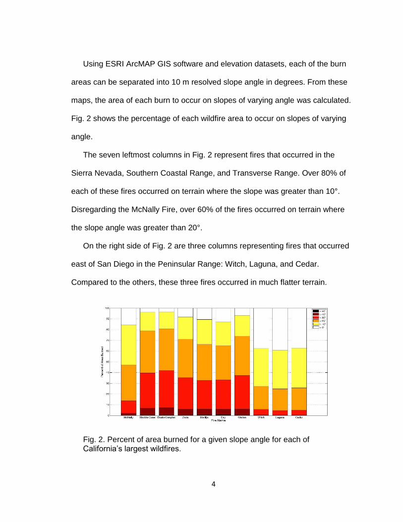
Using ESRI ArcMAP GIS software and elevation datasets, each of the burn

areas can be separated into 10 m resolved slope angle in degrees. From these

maps, the area of each burn to occur on slopes of varying angle was calculated.

Fig. 2 shows the percentage of each wildfire area to occur on slopes of varying

angle.

The seven leftmost columns in Fig. 2 represent fires that occurred in the

Sierra Nevada, Southern Coastal Range, and Transverse Range. Over 80% of

each of these fires occurred on terrain where the slope was greater than 10°.

Disregarding the McNally Fire, over 60% of the fires occurred on terrain where

the slope angle was greater than 20°.

On the right side of Fig. 2 are three columns representing fires that occurred

east of San Diego in the Peninsular Range: Witch, Laguna, and Cedar.

Compared to the others, these three fires occurred in much flatter terrain.

Fig. 2. Percent of area burned for a given slope angle for each of California’s largest wildfires.

5

Nevertheless, over 25% of these burns occurred on slopes greater than 20°.

Therefore, in California, the largest wildfires are linked to complex terrain.

While it remains mostly unchanging, terrain has a considerable, and often

unpredictable, effect on the atmosphere, the most variable and important

parameter in fire behavior. Therefore it is critical that research be performed to

understand how the atmosphere and terrain interact and how this interaction

affects fire spread.

With the use of computer models and laboratory experiments, significant

progress in fire science research has been made. Rothermel (1972) proposed

and published a mathematical model for the spread of fire by wind and slope. His

attempt was based on a simple empirical model with both wind and slope aligned

in the same direction. Albini and Baughman (1979) used the Rothermel model to

study the relationship between wind speeds and forest canopies. Their research

concluded by listing several limitations of the model, including that there was no

accounting for the interactions between the atmosphere and the fire. Later, a

vector form of the model would allow for non-uniform winds and slopes to be

used (Rothermel 1983). Many fire spread models today still rely on Rothermel’s

model, including BEHAVE (Andrews 1986) and FARSITE (Finney 1998). These

models rely heavily on statistics for predicting fire behavior, but can still be a

good tool for quickly predicting the movement of the fire under simple wind

regimes.

6

Current research in fire spread is focused on using models that couple the fire

and atmosphere and collecting observations to help evaluate the models.

Clements et al. (2007) collected the first high temporal, in situ, observational

dataset of meteorological conditions during a grass fire in flat terrain. An array of

instrumentation mounted on a 42 m tower captured 1 to 20 Hz data as a wind-

driven head fire moved through the tower. Among the variables measured were

three-dimensional winds, fuel and plume temperatures, and net radiation.

Turbulence characteristics were calculated from the three-dimensional winds

(Clements et al. 2008). The turbulence kinetic energy was found to have

increased during the passage of the fire front to five times above ambient

conditions. Also, increased spectral densities in the lower frequencies of the w-

component of the wind were found. This indicated that fire induced horizontal

eddies contributed a large amount to turbulence generation.

This dataset has been used to evaluate the output from many coupled fire-

atmosphere numerical models (Kochanski et al. 2013, Filippi et al. 2013).

Clements et al. (2008) also showed that the observed surface winds in and

around the fire front fit well with the numerical simulations of Cunningham and

Linn (2007). Kochanski et al. (2013) also performed a comparative analysis using

numerical output from the WRF-SFIRE model. After making small adjustments to

the model, he concluded that there was overall agreement on spread rates,

temperature profiles, and horizontal and vertical winds. Kochanski et al. stressed

7

that care should be taken when comparing single point observations to gridded

model data.

Several studies have focused on fire spreading on slopes using numerical

models. Linn et al. (2007) used HIGRAD/FIRETEC to run ten simulated wildfires

in various terrain types. It was found that fire behavior in varying complex terrain

is strongly linked to the coupling between the atmosphere and the terrain. In a

following paper, Linn et al. (2010) compared fire spread on flat terrain to sloped

terrain in varying fuel types with ideal atmospheric conditions. From these

simulations, several conclusions were reached. In addition to the faster spread

rates, the shape of the head fire was more pointed on the sloped terrain. It was

also noted that the effect of the slope is compounded as a head fire moves uphill.

This was the result of an increasingly pointed fireline. As the point of the fireline

increased on the slope, the angle between the slope and fire decreased, limiting

air entrainment from upslope and increasing the entrainment from downslope.

This caused a feedback in which the head of the fire tilted further, increasing

entrainment from downslope, and allowing the head of the fire to spread faster.

Additionally, fire spread rate on the sloped terrain varied greatly with changes in

fuel type.

Laboratory experiments have shown that fire occurring on a slope can spread

multidirectionally and can be adequately explained using wind and slope vectors

(Viegas 2004). Viegas also noted that wind began to affect the spread of the fire

more than the slope 40 seconds after ignition. This suggested that feedback from

8

the fire-atmosphere interactions had begun to influence fire spread more than the

terrain. Simpson et al. (2013) explored atypical fire spread on a leeward slope

with varying fuels using WRF-Fire. He proposed that interactions between pyro-

convection and terrain-modified winds produce updrafts and downdrafts, which

propagate back and forth across the fire front. As they cross the fire front,

vorticity driven circulations coupled with the updrafts and downdrafts, increasing

lateral fire spread across the slope. These simulations were performed under

idealized conditions.

To date, there have been essentially no comprehensive meteorological

measurements made of fire-atmosphere over slopes with the exception of

Clements and Seto (2015) which was a simple exploratory experiment with

limited measurements. Further field measurements will support model

improvements and aid in verifying theory in the area of wildfire micrometeorology.

This thesis presents new observations and the results of a field campaign in

which fire behavior was observed in complex terrain during an experimental fire.

In Chapter 2, the overall experimental design, site characteristics, and the

meteorological instrumentation layouts are described. Chapter 3 presents

measurements of temperature-pressure perturbations at the fire front. While in

Chapter 4, the micrometeorological observations, including heat flux and

turbulence, are analyzed. And Chapter 5 describes the generation of vorticity

observed during the fire. Finally, the conclusions and summary are presented in

Chapter 6.

9

Chapter 2 - Experimental Design

2.1 Site Selection and Characteristics

The field experiment was conducted southwest of King City, CA, at the United

States Army Garrison Fort Hunter Liggett (Fig. 3). This region of California is part

of the Coastal Range, a mountain range extending for much of the Pacific

coastline. A benefit of conducting an experiment at Fort Hunter Liggett was that it

contains much mountainous terrain, thus providing many options for

experimental sites. Several sites were surveyed at Fort Hunter Liggett and two

were selected for experimentation.

The first selected site (Fig. 4) was on a southwestern facing slope within

Stony Valley. This site had grass fuels that were the most uniform. Fig. 5

contains a three- dimensional satellite image of the burn plot generated from

elevation data and displays the uniformity of the slope at the site. The plot had a

Fig. 3. Regional road map of west central California. Inset shows satellite view with road overlay of United States Army Garrison Fort Hunter Ligget (Google Maps, 2016). First and second sites marked and labeled in inset.

10

Fig. 4. Map of experimentation site. The orange circle marks the location of the Doppler lidar. The green and red circles mark the miniature sodar and CSU-MAPS tower respectively. The red star shows the general location of the helicopter. Figure produced by Braniff Davis and used with permission.

Fig. 5. 3D image of the burn plot generated from elevation data. Elevation contours are plotted across the slope. The location of the three towers on the slope is shown. Towers are not to scale. Camera locations are marked by red dots. Overlaid satellite image provided by Google Maps (2015). Figure produced by Braniff Davis and used with permission.

11

slope angle of 20° and an area of 6.0x104 m2. The burn plot, detailed in Fig. 6,

was located on an isolated low ridge and with shallow drainage channels.

A second experiment site was selected within Stony Valley. This site was on

a taller mountain, with less uniform terrain and fuels. As a result, this site was not

as heavily instrumented as the first site. This thesis will primarily focus on data

and results from the first site.

The Stony Valley and surrounding lands of the garrison are an active

bombing range, making the region highly prone to accidental munitions ignitions.

Fig. 6. Detailed map of the burn area. The burn plot area is shaded by diagonal red lines. The red triangles represent tower locations. Purple circles mark the location of each of the fire sensor packages. The blue circles are the location of the RAWS stations. And the green squares show the location of the cameras. Figure produced by Braniff Davis and used with permission.

12

For this reason, the garrison is managed by prescribed fire, typically occurring

during late spring to early summer.

2.2 Field Experimental Design

The field experiment was designed to capture phenomena pertaining to the

interactions between the fire front and atmosphere on a simple and constant

slope in uniform fuels. These conditions would be the most ideal for comparing

numerical modeling with field observations. Fire-atmosphere interactions include,

but are not limited to, fire induced heat fluxes, plume circulations, temperature

and pressure perturbations due to the fire, vorticity generation, and fire-induced

circulations (Potter 2012a, 2012b).

There are two forms of measurement, direct and remote sensing. Direct

measurements of the propagating fire front were conducted by in situ instruments

along the slope from steel tower platforms. These sensor are required to be

capable of vertical and horizontal measurements and have a high temporal

resolution in order to capture fine-scale meteorological phenomena. Additionally,

they must be highly resistant to extreme heat.

Remote sensing measurements refer to instruments that are capable of

measuring at a distance. Instruments capable of this form of measurement

generally operate by measuring a portion of the electromagnetic spectrum. This

type of instrumentation can conduct higher spatial and temporal resolution

measurements in locations that cannot otherwise be reached. These

measurements can target meteorological phenomena, the ambient atmospheric

13

conditions, or any unique flow features associated with the local terrain and

environment. In this experiment, remote sensing instrumentation made

measurements of the smoke plume, the atmosphere surrounding the burn plot,

and the ambient atmospheric conditions. Additionally, video and photographic

observations were made from ground-based and aerial platforms to capture fire

behavior properties and rates of spread.

2.3 Micrometeorological Measurements

Three 10 m guyed steel towers were constructed on the burn plot along the

fall line of the slope (Fig. 5) to measure both meteorological and fire behavior

properties during the fire front passage (FFP). Each tower is referred to by the

position it had on the slope: bottom, middle, and top, which are referenced in Fig.

7. The bottom tower was placed on a flat section near the boundary where the

terrain transitions from flat to a 20° slope, approximately 40 m from the ignition

line. The bottom tower had an elevation of 436.5 m above mean sea level (MSL).

The middle tower was placed 71.2 m up the slope from the bottom tower and had

an elevation of 458.8 m MSL, a difference in height of 22.3 m from the bottom

tower. The top tower was placed 27.7 m upslope from the middle tower and had

an elevation of 468.1 m MSL, a difference in elevation of 9.3 m from the middle

tower.

Each of the three towers was equipped with an array of instrumentation

designed to measure several aspects of fire-atmosphere interactions. Table 1

details the sensor model numbers used on each tower. The three-dimensional

14

wind components were measured using 3D sonic anemometers (Applied

Technologies, Inc., Sx-probe) (Fig 7). Radiative heat fluxes were measured with

heat flux radiometers (Medtherm Corp, Model 64), also seen in Fig. 7. Near-

surface thermodynamic profiles were recorded utilizing an array of fine-wire

thermocouples mounted in 1 m increments on each tower. Atmospheric surface

pressure was measured at each tower using a barometer (R. M. Young, 61302)

mounted at two heights (3 and 9 m AGL) on the bottom and middle towers and at

one level, 3 m AGL, on the top tower.

Data were collected and stored on a Campbell Scientific Inc. (CSI) CR3000

datalogger. The clock on each datalogger was synchronized using a GPS sensor

Fig. 7. Photo of the burn area, pre-burn. Towers and instrumentation labeled. Pressure-temperature sensor locations indicated by red circles.

15

Table 1. Uniform sensors per tower

(Garmin, GPS16X), which received timestamps from satellite for each record.

Power was supplied by a pair of 12V deep cycle batteries wired in parallel. All of

this equipment was mounted near the base of the tower and required protection

from the fire. A fire resistant material, which resists emitted radiation, was

wrapped around the base of each tower, including the datalogger and battery

enclosures.

The 3D sonic anemometers were mounted on each tower to measure three-

dimensional wind and turbulence characteristics before, during, and after the

FFP. Sonic anemometers utilize transducer pairs, which measure the time

needed for sonic pulses to reach one another. The wind moving through the

sensor affects the speed of the sonic pulse, allowing for the quantification of u-,

v-, and w-components of the wind, as well as the virtual temperature of the air,

called sonic temperature. Additionally, the sonic anemometers have a high

temporal resolution and were sampled at a rate of 10 Hz. This interval was

Instrument, Model Height(s)

Variables Measured

Sampling Rate

3D Sonic Anemometer,

Sx-probe 9 m

u, v, w wind velocities and Sonic

Temperature

10 Hz

Heat Flux Radiometer,

Model 64 6 m

Radiative Heat Flux

10 Hz

Type T Thermocouples,

5SC-TT-40

1,2,3,4,5,6,7,8,9 m

Temperature 1 Hz

Barometer, 61302 3 m Pressure 1 Hz

16

needed in order to calculate turbulence statistics associated with the fire-induced

winds. The sonic anemometers were mounted at a height of 9 m and extended

~1-2 m outward from the tower to minimize any influence from the tower.

Heat flux radiometers were used to measure the upwelling radiative heat flux

from the fire front and were mounted on the bottom two towers. These sensors

were mounted at a height of 6.0 m AGL and extended ~1-2 m outward from the

tower. Radiative heat flux (Medtherm Corp, Model 64) sensors measure only the

radiative component of the heat flux by using a sapphire window over the sensor

surface. The bottom tower was additionally equipped with a second type of

radiometer, a total heat flux sensor (Hukseflux, SBG01). The total heat flux

sensor measures both the convective and radiative components of heat flux. All

of the radiometers faced downward in order to measure the heat being emitted

vertically from the fire front. And like the sonic anemometers, the radiometers

were sampled at a rate of 10 Hz.

A 10 m thermodynamic profile was measured at each tower using a

thermocouple array. The thermocouples are a fine-wire, type-T (Omega Inc.,

5SC-TT-40). The thermocouples were arranged in 1 m increments beginning at 1

m AGL and rising to the top of the tower. Thermocouples were sampled at a rate

of 5 Hz.

Two remote automated weather stations, hereafter referred to as RAWS,

were installed at locations on the ridge top and near the ignition line (Fig. 6). The

ridge top RAWS was equipped with a 3D sonic anemometer, sampling winds at a

17

rate of 10 Hz, and a thermocouple array, sampling temperatures at 1 Hz. The

RAWS near the ignition line was equipped with a R.M. Young 03002 Wind Sentry

cup anemometer and vane and a CSI CS215 temperature and relative humidity

probe. The data collected at this station was sampled at 1 Hz and averaged over

a 5 minute period.

An additional RAWS was situated on the ridge of site 2 and collected wind

and temperature data in 5 minute intervals. The purpose of this RAWS was to

collect data pertaining to the regional synoptic scale flow. This data was collected

for three months prior to the experiment.

An array of 13 Fire Sensor Packages (FSP) was installed in a grid within the

burn plot. The FSPs measured atmospheric pressure, external temperature, and

internal temperature. Each FSP contained a type E thermocouple, an aneroid

barometer, and a GPS. Each were sampled at 1 Hz. The FSPs were mounted on

steel T-posts at a height of 3 m. The distance between each of these sensors

was 10 m. The sensors in this grid were arranged in two rows and a single

column. The two rows were 20 m apart. The column ran down the center of the

two rows. This arrangement is shown in Fig. 6.

Video footage was captured using high-definition camcorders, marked by

green squares in Fig. 4. A ground-based unit was situated across the road from

the ignition line. This camera’s frame was fixed and encompassed all three

towers. An airborne camera (Fig. 8) filmed the experiment from a helicopter,

hovering approximately at 300 m AGL. Footage from the airborne camera was

18

not stationary due to movements made by the helicopter, but the framing of the

picture was broad enough to capture the entire burn plot.

2.4 Ambient Meteorological Measurements

Ambient meteorological conditions were measured up wind from the burn plot

and near the valley center by a Doppler miniSodar (Atmospheric Systems

Corporation, 4000 Series) and a 32 m mobile meteorological tower (Figs. 4, 9).

The sodar measured u-, v-, and w-components of the wind at heights between 20

and 200 m AGL in increments of 5 m. It also collected backscatter data from

each of these heights. Data from the sodar was averaged over a 10 minute

period and provided mean wind profiles of the surface layer and lower boundary

layer. The 32 m mobile tower was equipped with a 2D sonic anemometer (Gill,

Windsonic) and a temperature and relative humidity probe (Vaisala, HMP45C) at

heights of 7, 12, 22, and 32 m AGL. Sensors were sampled at 1 Hz and data

Fig. 8. Aerial imagery of the (a) ignition line and fire front passage at the (b) bottom, (c) middle, and (d) top towers.

19

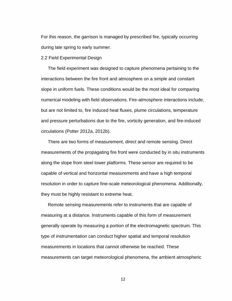
were averaged to 1 minute. The mobile meteorological tower was described in

more detail by Clements and Oliphant (2014).

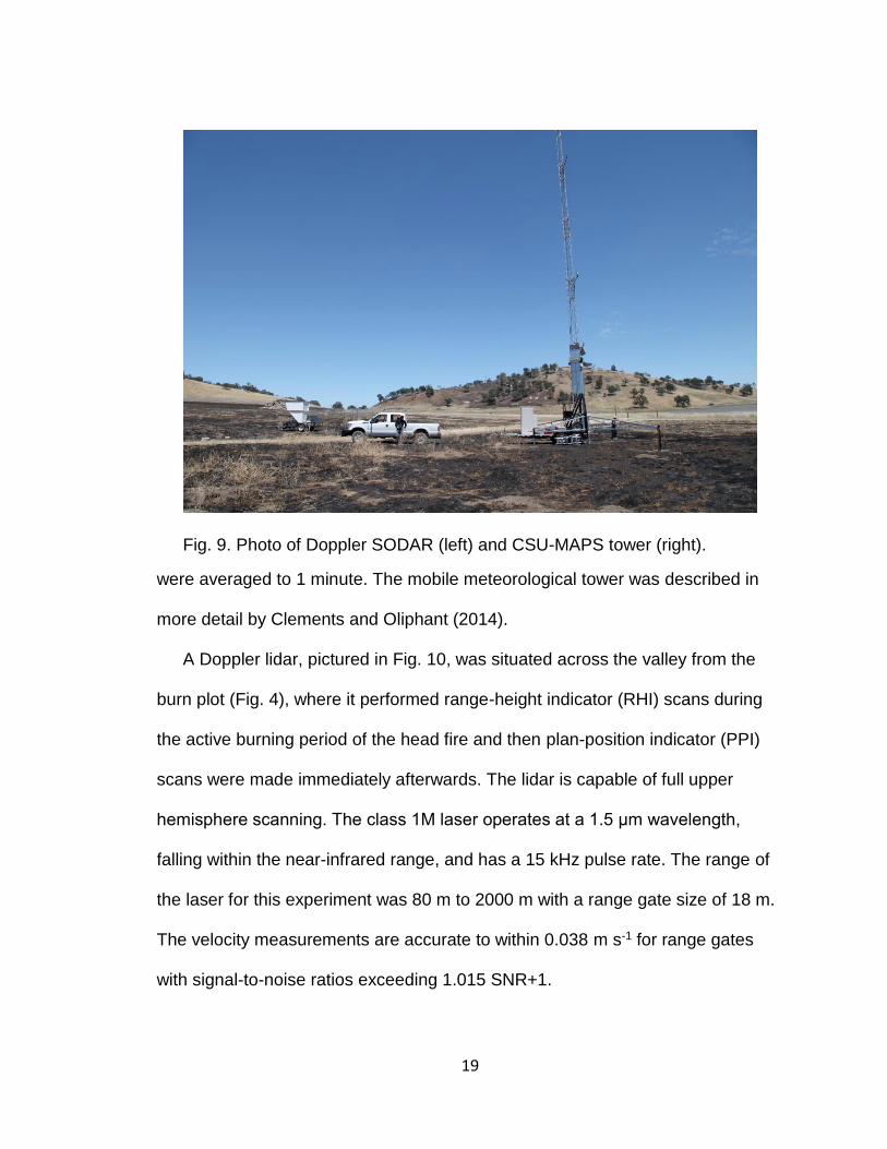
A Doppler lidar, pictured in Fig. 10, was situated across the valley from the

burn plot (Fig. 4), where it performed range-height indicator (RHI) scans during

the active burning period of the head fire and then plan-position indicator (PPI)

scans were made immediately afterwards. The lidar is capable of full upper

hemisphere scanning. The class 1M laser operates at a 1.5 μm wavelength,

falling within the near-infrared range, and has a 15 kHz pulse rate. The range of

the laser for this experiment was 80 m to 2000 m with a range gate size of 18 m.

The velocity measurements are accurate to within 0.038 m s-1 for range gates

with signal-to-noise ratios exceeding 1.015 SNR+1.

Fig. 9. Photo of Doppler SODAR (left) and CSU-MAPS tower (right).

20

An upper-air sounding was made prior to ignition at 8:48 PDT near the site of

the lidar. A Vaisala Inc. DigiCora III MW31 sounding system and a RS92GPS

radiosonde was used. The sounding collected data at 1 Hz intervals and

measured temperature, humidity, barometric pressure, and position obtained

from an onboard GPS. Wind speed and direction are calculated from position of

the sonde and other variables are calculated in real-time from the sensor

measurements.

Fig. 10. Photo of Doppler LIDAR.

21

2.5 Synoptic Overview

The climatological synoptic setup in the western continental United States for

the month of June has been described by Davis and Walker (1992) to be in a

state of transition. During the month of May, at 500 hPa, it is common for the axis

of a ridge of high pressure to be located near the west coast of the United States.

Through June, this ridge shifted eastward over the Great Basin, and allowed a

more monsoonal regime to begin in July. The presence of the ridge on the west

coast is usually associated with light winds at all levels of the atmosphere.

The experiment was conducted on 20 June 2012. On that day at 500 hPa, the

axis of the ridge was located near the west coast of the United States (Fig. 11).

This upper level ridge supported weak winds throughout all levels of the

atmosphere over California. Although the 850 hPa map (Fig. 12) shows northerly

Fig. 11. The 12Z 500 hPa analysis from 20 June 2012. (Source: NOAA)

22

winds, the velocity of this wind was diminished by a weak pressure gradient. The

12Z surface map (Fig. 13) showed calm winds in central California. For these

reasons, terrain driven winds were expected to prevail at the experimentation

site.

Chapter 3 – Surface Temperature Pressure Perturbations

3.1 Introduction

3.1.1 Thermocouple Measurements

The heat released during the combustion cycle drives many

micrometeorological phenomena surrounding wildland fires, including strong

buoyancy-driven circulations. Therefore, temperature observations are critical for

analysis of fire-atmosphere interactions.

Measuring extreme heat is challenging, but a few methods have been

Fig. 12. The 12Z 850 hPa analysis from 20 June 2012. (Source: NOAA)

23

developed. One technique utilized satellites to estimate wildfire temperatures

(Dennison et al. 2006). By measuring total spectral radiance of the surface of the

earth and applying Planck’s equation, temperatures ranging from 225 to 1225 °C

have been observed.

Thermocouples have been the most feasible method of directly measuring the

air temperature surrounding a fire. Thermocouples are durable, portable, and

relatively inexpensive. Clements (2010) directly observed the thermodynamic

structure of a fire plume in a grass fire using fine-wire thermocouples. He

observed a maximum temperature of 292.5 °C at 4.5 m AGL.

Several issues must be considered when using a thermocouple in the vicinity

of fire. Walker and Stalks (1968) showed that errors in the maximum temperature

are produced which are dependent on the gauge of the thermocouple. Bova and

Fig. 13. The 12Z surface analysis from 20 June 2012. (Source: NOAA)

24

Dickenson (2008) concluded that, if calibrated, data from thermocouples can be

useful for estimating fireline characteristics, though comparing thermocouple data

between wildfire studies is difficult as device type and deployment style are rarely

consistent. In a review of wildfire measurement, Kremens et al. (2010) point out

that temperatures observed within the radiation field by thermocouples are

dependent on both the characteristics of the measuring device and the fire. Even

with these issues, the thermocouple is an inexpensive method of broadly

measuring air temperature spatially and temporally in the fire environment.

3.1.2. Hypothesis

Due to the negative pressure tendency and the extreme heat at the fire front,

a negative covariance between pressure and temperature was expected. It was

hypothesized that the strength of a fire-atmosphere interaction could be analyzed

from the covariance of temperature and pressure.

3.2 Methods and Data Processing

The grid of FSPs was arranged as shown in Fig. 6. The layout was designed

to capture the temperature and pressure associated with a spreading fire front by

allocating enough points in the lines parallel and perpendicular to the hillside.

While a rectangular design would have been preferable, the limited number of

FSPs prevented a desirable resolution in both planar directions. The FSPs were

placed at a ten-foot grid spacing.

Data were stored on a micro SD card within each FSP. The hard drive was

capable of storing up to eight hours of data. The sensors sampled at a

25

rate of 1 Hz.

Calibration of the sensors was performed during the post processing of the

data. A mean of the ambient conditions was found using data from all of the

sensors. The mean temperature and pressure were found to be 32.25 °C and

959.7 hPa. Means were also calculated for each individual sensor. The

difference between the individual and composite means was then added to all

data points. Table 2 shows the adjustments that were made to the data from

each sensor.

Next, the temperature and pressure data were separated into the mean and

deviations from the mean:

T = T̅ + T′

P = P̅ + P′

T̅ is the representation of the temperature of the ambient atmosphere, or the

mean temperature with no influence from the fire. The mean temperature would

Table 2. FSP IDs and offsets made to each dataset

Sensor ID Number Temperature Calibration (°C)

Pressure Calibration (hPa)

04 -0.3603 -0.0256 08 0.2358 0.3763 09 0.2599 -0.7178 10 0.2795 0.0290 11 0.2592 -0.0926 12 -0.1839 -0.4016 13 0.3548 -0.1187 14 0.3194 -0.1585 15 -0.4948 0.2902 16 -0.0978 0.3383 17 0.2578 0.2185 18 -0.0128 0.0749 19 -0.8168 0.1877

26

ideally be calculated from a collocated sensor not exposed to the fire. But for this

experiment, no such sensor was in place. Therefore, the mean temperature was

calculated from a composite of all temperature observations in the grid for the

hour prior to the experiment. Next, by subtracting the mean temperature from the

observed, the temperature perturbations were found.

Because pressure was sampled at a rate of 1 Hz, and pressure data are

affected by changes in voltage input, consecutive samples could change by as

much as 0.2 hPa. To deal with this issue, the data were processed with a simple

averaging scheme, in which data were smoothed by averaging the five data

points before and after each point in the time series.

To determine the pressure deviations, a linear de-trending method was

utilized following Burba and Anderson (2010). First, a portion of each time series

must be selected containing the data associated with the FFP. The FFP lasted

no longer than 1 minute at each FSP. Therefore, for each FSP, a data window

associated with the FFP was defined as the 30 seconds before and after the

maximum temperature in the time series. At the beginning and end of each 1

minute data window, a 1 minute average pressure was computed. A trend line

was fit between these two averaged points, and used to define P̅ during the time

of FFP. The pressure perturbation, P’, was then calculated as the difference

between the trend line and actual pressure measured during FFP.

The covariance between temperature and pressure, T′P′̅̅ ̅̅ ̅, was found by

calculating the product of the deviations and averaging over time. For this

27

purpose, a three second Reynold’s averaging period was used on the product of

the deviations.

Calculating the covariance between temperature and pressure has an

additional analytical benefit. Within the pressure data, there are increases and

decreases not associated with the fire. To distinguish between the fire induced

and non-fire induced changes in pressure, the covariance uses the temperature

deviation from the mean, T’. In ambient conditions, T’ is approximately zero. This

reduces the product of T’ and P’ to a negligible value, thus eliminating the non-

fire induced changes in pressure.

3.3 Results and Discussion

3.3.1 Rate of Spread

The timing of maximum temperature during FFP at each FSP provides an

estimate of the fire rate of spread across the grid area. Rate of spread is the

amount of time it takes for a fire to propagate across an area. FFP occurred at

each of the thirteen grid FSPs during a 6 minute period lasting from 11:22:00

PDT through 11:28:00 PDT, which was determined by the observed temperature

maxima.

Fig. 14 shows a time series of temperature from each FSP. It can be seen

that as the fire front progressed across the grid, the observed maximum

temperatures increased. A peak in maximum temperatures was reached just as

the fire front passed the last two FSPs. This suggests that the development of

the fire front was completed by this time. Since the direction of fire spread was

28

south-southwest to north-northeast across the sensor grid, estimates could only

be made from sensors along the same alignment. Fig. 15 shows estimates made

from the sensors following this orientation.

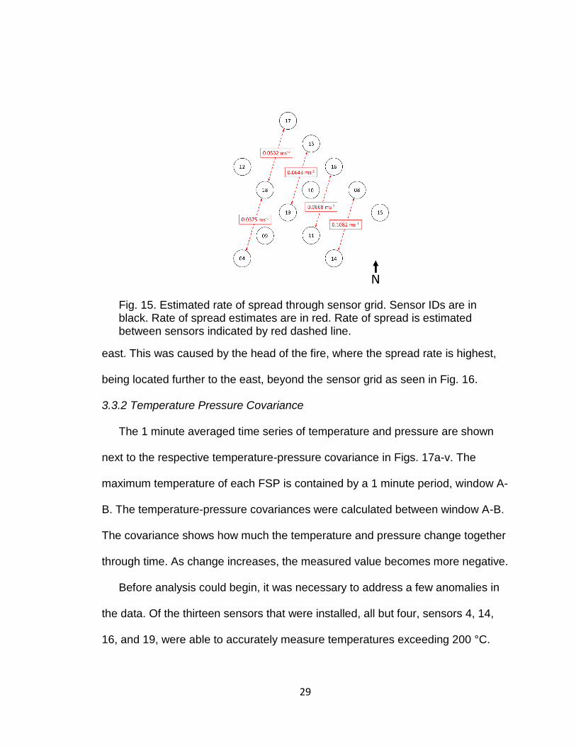
These estimates show that the rate of spread increased as the fire front

progressed across the west end of the burn plot. From sensor 04, near the

ignition line, to sensor 18, the rate of spread was 0.04 m s-1. From sensor 18 to

sensor 17, near the back of the grid, the rate of spread was 0.05 m s-1. This was

an increase in the spread rate of 0.01 m s-1.

It was also observed that the spread rate increases from west to east. The

spread was slowest on the western end of the grid where the rate of spread was

0.05 m s-1 between sensors 18 and 17. The rate of spread from sensor 14 to 8,

on the eastern end, was 0.10 m s-1. This is a difference of 0.05 m s-1 from west to

Fig. 14. Temperature time series from each of the FSPs in the grid.

29

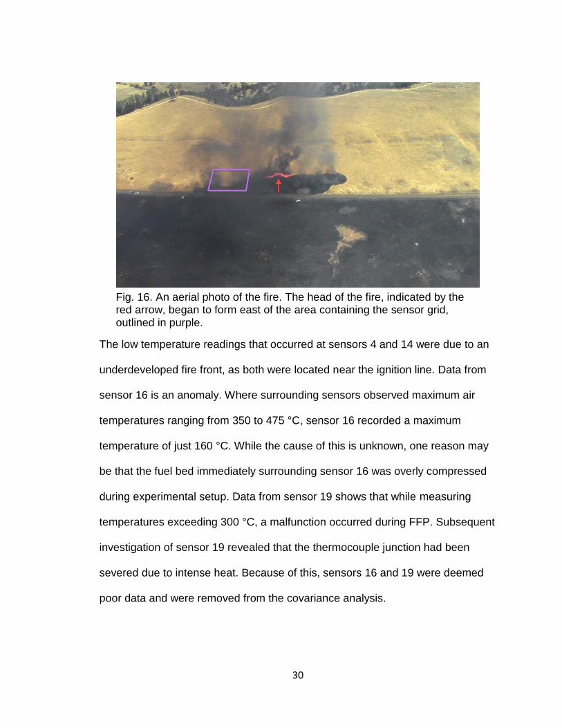
east. This was caused by the head of the fire, where the spread rate is highest,

being located further to the east, beyond the sensor grid as seen in Fig. 16.

3.3.2 Temperature Pressure Covariance

The 1 minute averaged time series of temperature and pressure are shown

next to the respective temperature-pressure covariance in Figs. 17a-v. The

maximum temperature of each FSP is contained by a 1 minute period, window A-

B. The temperature-pressure covariances were calculated between window A-B.

The covariance shows how much the temperature and pressure change together

through time. As change increases, the measured value becomes more negative.

Before analysis could begin, it was necessary to address a few anomalies in

the data. Of the thirteen sensors that were installed, all but four, sensors 4, 14,

16, and 19, were able to accurately measure temperatures exceeding 200 °C.

Fig. 15. Estimated rate of spread through sensor grid. Sensor IDs are in black. Rate of spread estimates are in red. Rate of spread is estimated between sensors indicated by red dashed line.

30

The low temperature readings that occurred at sensors 4 and 14 were due to an

underdeveloped fire front, as both were located near the ignition line. Data from

sensor 16 is an anomaly. Where surrounding sensors observed maximum air

temperatures ranging from 350 to 475 °C, sensor 16 recorded a maximum

temperature of just 160 °C. While the cause of this is unknown, one reason may

be that the fuel bed immediately surrounding sensor 16 was overly compressed

during experimental setup. Data from sensor 19 shows that while measuring

temperatures exceeding 300 °C, a malfunction occurred during FFP. Subsequent

investigation of sensor 19 revealed that the thermocouple junction had been

severed due to intense heat. Because of this, sensors 16 and 19 were deemed

poor data and were removed from the covariance analysis.

Fig. 16. An aerial photo of the fire. The head of the fire, indicated by the red arrow, began to form east of the area containing the sensor grid, outlined in purple.

31

The covariance between temperature and pressure was expected to have a

negative correlation during FFP. The sign of the covariance is dependent on the

pressure deviation. The reason for this is because the temperature deviation will

always be positive during FFP.

Sensors nearest the ignition line, 4, 9, and 14, observed the weakest

covariance during the FFP, -3.6, -3.2, and -0.1 °C hPa respectively. At sensor 4,

where the maximum temperature only reached 112.9 °C (Fig. 17a), the negative

covariance was strongly dependent on the negative pressure deviation. Sensor 9

Fig. 17a-f. Temperature and pressure time series with covariance plots for the duration of the fire front passage for sensors 04, 08, and 09 respectively.

(a) (b)

(d) (c)

(e) (f)

32

Fig. 17g-n. Temperature and pressure time series with covariance plots for the duration of the fire front passage for sensors 10, 11, 12, and 13 respectively.

(m)

(k)

(i)

(g)

(n)

(l)

(j)

(h)

33

Fig. 17o-v. Temperature and pressure time series with covariance plots for the duration of the fire front passage for sensors 14, 15, 17, and 18 respectively.

(t)

(o)

(u)

(q)

(s)

(v)

(r)

(p)

34

had a maximum temperature of 272.3 °C (Fig. 17e). Although this temperature

was well above what was observed at sensor 4, a weak pressure deviation

resulted in similar covariance values. Sensor 14 had the smallest temperature

maximum, which was a result of being near the ignition line. The pressure did

drop during the FFP, but the mean pressure during the FFP was much lower

than the drop in pressure. This resulted in a very weak covariance during FFP at

sensor 14.

The strongest covariance values were observed at sensors 12 (Fig. 17l) and

15 (Fig. 17r), -17.4 and -16.4 °C hPa, respectively. Maximum temperatures at

these two sensors were 427.6 and 312.0 °C, respectively. The pressure

deviations at each of these two stations contrast one another. Sensor 12 shows

the greatest pressure deviation, while having a lower temperature measurement.

This would suggest that, while there is a link between these two variables during

FFP, the intensity of the heat has no correlation with drop in pressure.

The remaining sensors, 08, 10, 11, 13, 17, and 18, observed covariance

strengths ranging from -6.1 to -11.2 °C hPa. Maximum temperatures at these

sensors varied due to the dynamic fire front. While each sensor shows a strong

negative temperature-pressure covariance during FFP, the results of this

experiment remain unclear.

The covariances show how much temperature and pressure change with one

another. While each sensor observed strong negative covariances, the strength

of the covariance during FFP at each sensor varied throughout the grid. This

35

indicates, for this data set, that there is no clear relationship between

temperature and pressure at the fire front.

There are a few reasons why the results are unclear. First, wind is a primary

cause of fire front type. A backing fire and head fire would impinge on the

sensors differently. For light winds particularly, without knowing the wind direction

at each sensor, it cannot be known how the fire impinged on each sensor. This

could be resolved by equipping each FSP with a sonic anemometer.

Second, as seen with sensor 16, fuel uniformity can greatly affect the

measurement. One observation that can be made is that, with the exception of

sensor 14, the strongest covariances were observed at the sensors on the edge

of the grid. The fuels surrounding these sensors were the least affected by the

installation. For future experiments, it would be ideal to install sensing equipment

before vegetative growth begins. This would allow for greater fuel uniformity

during an experiment.

3.4 Conclusion

In summary, a negative covariance between temperature and pressure was

expected at the fire front due to intense heating from the fire and a negative

pressure tendency caused by rising air at the fire front. Because of the location of

the grid in relation to the ignition line, the fire had not fully intensified before

reaching the sensors, as observed in Fig. 14. Additionally, the magnitude of the

covariances varied greatly across the grid, showing no clear relation between

temperature and pressure at the fire front.

36

While the data does show that the technique and hypothesis have promise,

further testing is needed. Future experiments will need to be well planned and

feature additional sensors on the FSPs. Data from FSPs on a consistent and

completely developed fire front would be a good comparison for the covariances

from this experiment. Another option would be to make observation in a wind

tunnel, where wind speed and direction, as well as fuel uniformity, can be

controlled.

Chapter 4 – Micrometeorology

4.1 Introduction

The interactions between a fire, the atmosphere, and surrounding topography

display a wide range of complexity. Therefore, it can be difficult to provide timely,

reliable information to firefighting crews. Computer models operating using the

Rothermel fire behavior model (Rothermel 1972), such as Farsite (Finney 1998)

and BehavePlus (Andrews 1986), forgo many of the complex physical

interactions that occur in the wildfire environment. Instead, they opt for

computational efficiency, using only crucial variables to empirically estimate fire

behavior. The problem with this technique is that it ignores many meteorological

processes affecting fire behavior.

With the introduction of coupled fire-atmosphere models, fully three-

dimensional fluid dynamical processes have been applied to fire behavior

prediction. Kochanski et al. (2013) used WRF-SFIRE to simulate and compare

the fire behavior to the observations collected during the FireFlux experiment

37

(Clements et al. 2007). The results of the study were encouraging, as

comparisons between the model rate of spread, thermodynamic profiles, and

three-dimensional winds were close to observed. These studies were conducted

on flat terrain, which removed many of the complications that occur with the

addition of slope.

There have been many modeling studies that have simulated fire behavior in

complex terrain, but few observational datasets currently exist that can evaluate

the simulated results. Linn et al. (2007) explored the extent to which the fire and

atmosphere were coupled in various complex terrain scenarios. This study used

several terrain types with varying ambient wind speeds. Results showed that the

effect of the mean wind on the fire spread distance on flat terrain was

approximately equal to that of fire spread on a canyon sidewall where the mean

wind was obstructed by the opposite canyon sidewall. Simpson et al. (2013)

investigated the fire spread on a leeward mountain slope using four different

WRF-Fire simulations. The simulations used two fuel types were used and were

conducted with both coupling and non-coupling of the fire and atmosphere.

Results showed that for each case, the fire spread was initially predominantly

upslope, but when the fire reached the ridge top, the fire spread was halted by

the cross-ridge winds, and forced to spread laterally across the slope. Simpson

et al. (2014) called this fire spread phenomenon vorticity-driven lateral fire spread

(VLS) and hypothesized that it was caused as a result of vorticity that formed in

the lee of the ridge line.

38

In this chapter, the results of the micrometeorological observations will be

described. Analysis of in situ sonic anemometer data will be conducted and

compared to video imagery and Doppler lidar observations made during the

experiment. First, data obtained during the FFP at each of the three towers will

be explored followed by other observations of unique events that occurred.

4.2 Data Processing

To determine the influence of terrain-induced winds on the fire as it spreads

up the hillside, data from each sonic anemometer were rotated into a slope-valley

coordinate system (Fig. 18). The valley component of the wind is represented by

u, where +u is directed up valley and –u is down valley. The v-component is

aligned along the slope, where +v is towards the slope and –v is away from the

Fig. 18. Slope-valley wind coordinate system

39

slope. The vertical velocities are the w-component of the wind. All vertical

velocities were tilt-corrected following Wilczak et al. (2001) to eliminate any

imprecise leveling of the sonic anemometer. All sonic data were run through a

despiking routine to remove any spurious data associated with noise (Lee et al

2004.). Despiking removed data points that exceeded four standard deviations

from the mean within a 2-minute moving data window. Any data points that were

removed were replaced with linearly interpolated values. Unrealistic spikes

during FFP were visually inspected as the turbulent nature of the atmosphere

during FFP often causes rapid fluctuations and spikes in wind velocities.

From the despiked and tilt-corrected 10 Hz data, each variable was then

separated into mean and perturbation parts as follows:

u = u̅ + u′ v = v̅ + v′

w = w̅ + w′ T = T̅ + T′

where the overbar denotes the mean and the prime denotes the perturbation.

The mean was calculated from a 10 minute moving window and subtracted from

the instantaneous values to obtain the perturbations.

For temperature perturbations, values collected during the FFP at each tower

were removed from the time series. Had temperature data collected during FFP

been left in, the temperature mean would have increased by approximately 3 °C.

This would have lowered values of temperature perturbations and flux estimates.

Sensible heat flux and turbulent kinetic energy (TKE) were calculated from

each time series data set. Sensible heat flux (Hs) can be represented by

40

Hs = ρCpw′T′̅̅ ̅̅ ̅̅

where ρ is air density, Cp is heat capacity of dry air at constant pressure, and

w′T′̅̅ ̅̅ ̅̅ is the covariance between the vertical velocity and sonic temperature

perturbations.

TKE is a measure of the total kinetic energy per unit mass contained within

turbulent eddies in the atmosphere. It is equal to one half the sum of the three

velocity variances.

TKE

m=

1

2[u′2̅̅ ̅̅ + v′2̅̅ ̅̅ + w′2̅̅ ̅̅̅]

An analysis of turbulence spectra was also performed on the wind velocities

for each of the three towers before, during, and after FFP. The analysis used a

Morlet wavelet function to determine the spectral density of the turbulence across

frequencies (Torrence and Compo 1998).

4.3 Fire Front Passage

4.3.1 3D Wind and Sonic Temperature

Individual components of the wind velocity were plotted (Fig. 19) to show the

magnitude of each over the hour that the experiment was conducted. Before

ignition, between 11:00:00 to 11:18:00 PDT, both u and v values can be seen

trending between -3 and 4 m s-1 at the middle and top towers. The bottom tower

observed a sharp reversal of the u and v values at 11:16:00 PDT, and then

calmed to near 1 m s-1. The vertical velocity values at each tower were near

41

0 m s-1 and showed no trend. The average ambient temperature for this time

period was 30 °C.

Fire-induced winds began with the arrival of the fire front at the bottom tower

at 11:27:00 PDT. The maximum sonic temperature during this FFP was 287 °C.

The temperature then decreased to ambient levels as the fire passed the bottom

tower. Four minutes after the fire had passed, periods of high temperature were

again observed, which will be discussed later. Within the plume, vertical velocity

reached a maximum of 11.1 m s-1 at the bottom tower during the FFP.

Wind velocities during FFP at the middle tower were substantially weaker in

magnitude than those that occurred at the bottom tower. The FFP at the middle

tower occurred at 11:34:00 PDT. The maximum sonic temperature at this tower

was 95.2 °C. Negative vertical velocity values during FFP indicate that strong

downdrafts occurred at a time when rising motion was expected.

Fig. 19a-d. Time series of u, v, and w velocities, as well as sonic temperature for the bottom tower (blue), middle tower (red), and top tower (magenta).

(a)

(b)

(c)

(d)

42

The FFP at the top tower occurred at 11:46:00 PDT, and at this time the fire

had become a weak backing fire. The temperature of this FFP was the lowest of

the three towers, reaching only 58.2 °C. The maximum vertical velocity during

FFP at the top tower was 4.17 m s-1.

The ambient winds from two RAWS, set up on the perimeter of the burn plot,

were analyzed to understand FFP variability at each tower. One RAWS was

placed on the ridge above the burn plot and the other in the valley near the

ignition line. The mean wind was light and variable during the course of the

experiment as shown by the wind speed and direction (Fig. 20). From 11:15:00

PDT to 12:00:00 PDT, the wind speeds at both RAWS did not exceed 3 m s-1.

The wind directions, while mostly easterly, tended to oscillate between north and

south from 11:00:00 PDT through 11:30:00 PDT at both sites. These winds were

the cause of the irregular fire behavior that occurred during the first half of the

Fig. 20. Five minute averaged two meter wind speed at RAWS located in the valley (red) and ridge (black).

43

experiment. From 11:30:00 PDT onward, the wind direction became more

easterly at both RAWS, indicating that wind was coming over the ridge. This

caused the backing fire behavior that was observed during the second half of the

burn.

4.3.2 Turbulence and Sensible Heat Flux

Using the radiative heat flux plotted in Fig. 21, the period of FFP can be

determined for the bottom and middle towers. For the bottom tower, FFP began

at 11:27:00 PDT. The residence time of the fire was approximately 1 minute and

the FFP ended at 11:28:00 PDT. Elevated values of radiative heat flux continued

until 11:32:00 PDT.

The ambient micrometeorological conditions were vastly different than those

during FFP. For example, ambient levels of TKE ranged from 1 to 3 m2 s-2, but

during the FFP, when the fire passed the tower, TKE reached a maximum value

Fig. 21. Radiative heat flux measured at the bottom (blue) and middle (red) towers.

44

of 23 m2 s-2 (Fig. 22a). This increase was the result of fire-induced winds being

driven by the convective buoyancy above the fire front. Similarly, Hs reached a

maximum of 330 kW m-2 as the fire front passed, whereas ambient Hs before the

FFP was observed to be between -3 and 3 kW m-2.

To better understand which variance component dominated the TKE, a time

series of variance for each velocity component, Fig. 22b, is presented. From this

figure, it can be seen that the magnitude of vertical velocity variance during the

FFP was roughly 1.5 times greater than either u or v components. It can also be

seen that during the initial 20 seconds of FFP, the v and w velocities increased

much sooner than the u velocities. This was most likely the result of horizontal

Fig. 22. (a) shows the TKE and Hs observed at the bottom tower during FFP. (b) shows the velocity variances at the bottom tower during the same time frame.

(a)

(b)

45

shear generated near the boundary of the convectively buoyant plume. Because

the fire front was nearly parallel to the ridge top during the FFP at the bottom

tower, the u- component of the wind remained weaker as the fire approached.

The u- component of the wind increased only as the fire passed the tower, which

was the result of turbulence within the plume and fire-induced circulations that

resulted from instabilities in the plume.

Lidar measurements of backscatter and radial velocity during the FFP at the

first tower are shown in Fig. 23a. The data were processed following the

techniques outlined by Charland and Clements (2012). Black contour lines of

backscatter show the boundaries of the smoke column. These agree well with

the aerial video imagery captured at the same time (Fig. 23b). Figure 23b

indicates that the the smoke column became more vertical as the fire passed the

bottom tower. The radial velocities measured by the lidar may help explain the

cause of the upright plume. Southwesterly winds, areas colored yellow through

red, were observed on the valley side of the plume, whereas northeasterly winds

were observed on the ridge side. These two winds converged and the winds near

the plume weakened causing the plume to become more upright, rather than

being tilted over in the wind.

After the FFP had occurred at the bottom tower, several instances of negative

Hs were observed. The first negative value, approximately -45 kW m-2, occurred

directly after the maximum Hs was reached during FFP. The interpretation of the

negative heat flux is that warmer air was transported downward to the surface

46

from aloft. Following the FFP, three weaker instances of negative Hs occurred,

ranging from -10 to -20 kW m-2. Then at 11:31:30 PDT a second period of

negative Hs occurred which had a value of -50 kW m-2. The negative value of Hs

Z (m

M

SL)

Fig. 23. (a) RHI scan performed by the Doppler lidar during the FFP at the bottom tower. Warmer colors represent southwesterly wind, cooler colors are northeasterly. (b) corresponding aerial photograph.

(a)

(b)

47

indicates that heated air was sinking at this time. An associated increase in TKE

at this time was composed of elevated values in the v and w velocity variances.

Since FFP had already occurred at the bottom tower, these observations would

suggest a downslope wind was present and was transferring heat downslope

through the array of instruments on the bottom tower.

At the middle tower, the FFP began at 11:34:00 PDT and lasted for

approximately 1.33 minutes (Fig. 24). At this time in the experiment, downslope

winds had caused the fire to become a low intensity backing fire. As a result, the

spread rate decreased, leading to an extended period of FFP at the middle

tower.

Fig. 24. (a) shows the TKE and Hs observed at the middle tower during FFP. (b) shows the velocity variances at the middle tower during the same time frame.

(a)

(b)

48

No increase in Hs was observed during the FFP at the middle tower, rather a

value of -35 kWs-2 was observed. This would suggest that heat was being

transported downslope.

The magnitude of the TKE and Hs at the middle tower was substantially less

than that of the bottom tower. During FFP, the maximum TKE was measured to

be 5.7 m2 s-2, a value of 17.3 m2 s-2 less compared to the bottom tower. The

velocity variances during the FFP show roughly equal values, indicating that the

TKE was not driven by any specific component of the wind.

Lidar and aerial imagery during the FFP at the middle tower, Figs. 25a and

25b, provide better detail to the changes in the wind that occurred on the slope. It

can be seen in the lidar velocities that the wind over the plot had changed to a

northeasterly wind, replacing the southwesterly winds that existed during FFP at

the bottom tower. This caused dramatic decrease in the fire behavior, marked by

the significant decrease in Hs from the bottom tower to the middle tower. These

strong northeasterly winds forced air down the slope and tilted the smoke column

over the valley, as shown in both lidar data and aerial imagery.

In Fig. 24, several additional peaks in TKE were observed where no increase

in Hs was found. These TKE peaks occured during changes in the wind direction

on the hillside. The elevated values of TKE, beginning at 11:31:30 PDT, were

associated with a change in v-component velocities, as can be seen in the high

level of v’. Two higher TKE values were observed post FFP at 11:37:40 and

11:38:30 PDT. At each of these times, v’ contributed a large portion to the TKE.

49

The TKE at 11:37:40 PDT also contained a large portion of w’, which indicates

that the wind was following the terrain. The TKE at 11:38:40 PDT had higher

Fig. 25. (a) RHI scan from the Doppler lidar taken during FFP at the middle tower. Warmer colors represent southwesterly wind, cooler colors are northeasterly. (b) corresponding aerial photograph.

(a)

(b)

50

values of u’, signaling a cross-slope wind, not necessarilly following the terrain.

At the tower nearest the top of the hillside, the low intensity backing fire

continued. FFP at the top tower began at 11:46:30 PDT. The maximum Hs

observed during the FFP was 24.9 kW m-2 (Fig. 26a). The TKE observed during

the same time was not substantial enough to be distinguishable from ambient

conditions without comparing it with Hs.

During the FFP, maximum observed TKE was 3.9 m2 s-2. The velocity

variances at the top tower (Fig. 26b) show that, at the time of FFP, the primary

wind components contributing to TKE were the u and w wind velocities.

Fig. 26. (a) shows the TKE and Hs observed at the top tower during FFP. (b) shows the velocity variances at the top tower during the same time frame.

(a)

(b)

51

Several additional peaks in TKE are also seen in Fig. 26a. At 11:50:30 PDT,

TKE measured 5.7 m2 s-2 and Hs measured 13.6 kW m-2. By this time, the fire had

passed the tower and was located at a slightly higher position on the slope. The

cause of these elevated values of TKE and Hs can be seen in Fig. 19b. During

the time period from 11:50:00 to 11:51:00 PDT, a sharp decrease in the v wind

component was observed, indicating that a strong northeasterly gust had

occurred. This corresponds with the maximum in the v velocity variance, seen in

Fig. 26b.

Video imagery from the 11:49:00 to 11:52:00 PDT time period, shown in Fig.

27, indicates that smoke was being advected downslope at 11:51:00 PDT. Since

air is shown to be sinking downslope, and the sensible heat flux during the period

shows positive values, cool air sinking downslope was also considered a

possibility. This combination would also yield a positive heat flux. For this reason,

Fig 27. Four photos taken in 1 minute intervals depicting the downslope wind dispersing the smoke down the slope.

52

time series plots of T’ and w’ are shown in Fig. 28. From these figures, it can be

seen that elevated values of T’ correspond to positive values of w’ in the period

just prior to the downslope wind at 11:51:00 PDT. This agrees with the positive

values of sensible heat flux seen in Fig. 26a during the same period.

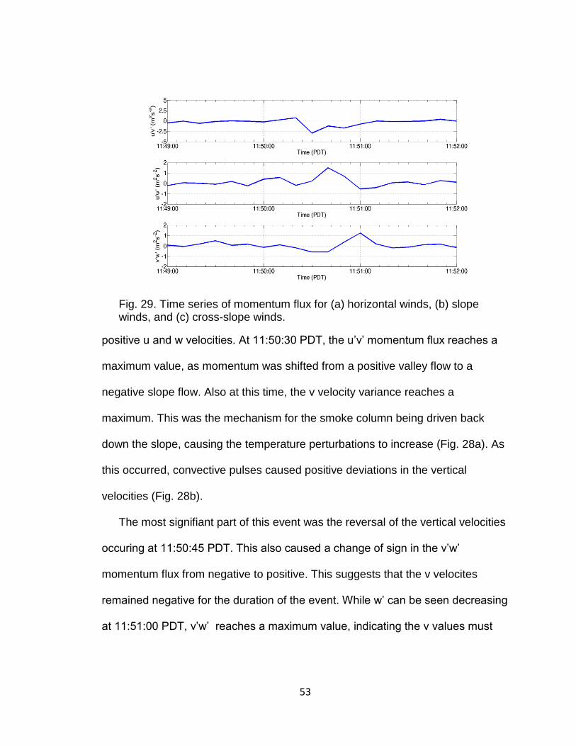
Momentum fluxes (Fig. 29) during the downslope wind period show how

momentum shifted through the three wind velocity components. One issue with

momentum fluxes presented in time series is that positive values can occur when

both momentum diviations are positive or both negative. Negative momentum

fluxes can occur when one variable is positive and the other negative, or vice

versa. For this reason, vertical velocity deviations seen in Fig. 28b can be used

to interpret the positive and negative values of the momentum fluxes. It can be

seen that until 11:50:00 PDT, no significant momentum fluxes occur (Fig. 29).

Just after 11:50:00 PDT, a slight transfer of momentum occurred between the

Fig. 28. Perturbation time series of sonic temperature (a) and vertical velocity (b) from the top tower during a downslope wind.

53

positive u and w velocities. At 11:50:30 PDT, the u’v’ momentum flux reaches a

maximum value, as momentum was shifted from a positive valley flow to a

negative slope flow. Also at this time, the v velocity variance reaches a

maximum. This was the mechanism for the smoke column being driven back

down the slope, causing the temperature perturbations to increase (Fig. 28a). As

this occurred, convective pulses caused positive deviations in the vertical

velocities (Fig. 28b).

The most signifiant part of this event was the reversal of the vertical velocities

occuring at 11:50:45 PDT. This also caused a change of sign in the v’w’

momentum flux from negative to positive. This suggests that the v velocites

remained negative for the duration of the event. While w’ can be seen decreasing

at 11:51:00 PDT, v’w’ reaches a maximum value, indicating the v values must

Fig. 29. Time series of momentum flux for (a) horizontal winds, (b) slope winds, and (c) cross-slope winds.

54

have become more negative. This result indicates that the downslope wind

transported smoke from the top of the ridge down into the valley (Fig. 27c).

4.3.3 Turbulence Spectra

Energy contained within turbulence is transported from larger eddies to

smaller eddies where it is dissipated (Šavli 2012). Šavli went on to show that

large eddies tend to be more intense than smaller eddies. And because the

larger eddies are more intense, they are capable of generating shear, thus

creating smaller eddies. An in depth analysis of turbulence spectra associated

with fire was performed on datasets from four field campaigns by Seto et al.

(2013). Their analysis of the horizontal velocity spectra showed that increases at

mid to high frequencies was most likely attributable to eddies shedding off of the

fire rather than ambient wind shear. The vertical velocity spectra increased

across all frequencies during FFP and the observed temperature spectra was

described as “white noise”, as it failed to follow the -2/3 inertial subrange slope

(Kolmogorov, 1941) in the higher frequencies.

The turbulence spectra for this campaign was separated into u, v, and w wind

velocities, as well as temperature (Figs. 30a-d). The velocity spectra were

normalized using friction velocity. The spectra are compiled from data

encompassing 9 minutes prior to and after the time of maximum temperature,

which represents the time of FFP. The 9 minute period was used because of the

extended duration of the FFP at the middle and top towers where the rate of

spread had decreased.

55

The u spectra are shown in Fig. 30a. The most notable features of these

spectra are the low frequencies, where the spectra at the bottom tower is

significantly lower than the other towers. Because the two upper towers were

exposed to the northeasterly wind above the ridge, they experienced a higher

level of wind shear, which elevated the lower frequency spectra.

The v spectra is shown in Fig. 30b. The v spectra of each tower at FFP were

fairly uniform with one another. Like the u spectra, much higher values were

obtained in the lower frequencies, indicating that larger eddies and wind shear

Fig. 30. Normalized power spectra during fire front passage at each tower for (a) u, (b) v, and (c) w wind velocities, as well as (d) sonic temperature. The bottom tower is in blue, middle in red, top in magenta.

(a)

(c)

(b)

(d)

56

were more dominant than the smaller eddies associated with the fire. A

significant increase in v velocity spectra was observed near 0.3 Hz at the bottom

tower during FFP, which was also found in the u spectra (Fig. 30a).

The vertical velocity spectra (Fig. 30c) displays the best example of the

difference between high and low intensity fire induced turbulence generation.

Higher intensity fire was observed at the bottom tower, while lower intensity was

observed at the middle and top towers. The turbulence spectra at the bottom

tower reached the highest values in the frequencies greater than 0.3 Hz. For

frequencies greater than 1 Hz, the energy associated with turbulence generated

by the fire front was a whole order of magnitude larger than that observed during

the lower intensity FFP.

4.4 Summary

The evolution of the fire spread can be better understood from the analysis of

the micrometeorological observations made at different location along the slope.

The maximum observed intensity occurred as the fire passed the bottom tower

where the slope was nearly flat with little inclination. Lidar data at this time

showed light southwesterly upslope winds and a nearly vertical smoke plume. As

the fire progressed upslope and passed the middle tower, lidar observations

revealed a strong reversal of the wind to a northeasterly downslope wind. This

slowed the forward spread of the fire and substantially weakened its intensity. At

this time, negative values of sensible heat flux were observed. This indicates that

heat and plume air were being transported downslope by the northeasterly winds

57

above the ridge. The low intensity backing fire continued slowly spreading up the

slope as it passed the top tower where the lowest heat fluxes and minimal fire-

atmosphere coupling were observed.

Chapter 5 – Vorticity Estimation and Fire Whirls

5.1 Introduction

Vorticity is described as the spin of air in the atmosphere about some axis,

vertically or horizontally. It is typically generated baroclinically, by shear stress, or

by body forces. Each of these three types of vorticity generation can be observed

in the atmosphere surrounding a wildfire (Forthofer and Goodrick, 2011).

Baroclinic vorticity is generated when the extreme temperature gradient between

the plume of the fire and the ambient air creates an imbalance with the vertical

static pressure gradient. The vorticity that is generated by this imbalance acts to

mix cool and warm air in an attempt to return the atmosphere to a static state.

Shear vorticity is generated by varying wind speeds. At the surface, this occurs

primarily due to frictional drag.

Vorticity can be modified via transport, axial tilt, or stretching. Fire whirls

provide the best example for each of these modifications. For a whirl to form,

either vertical vorticity needs to be stretched or horizontal vorticity needs to be

tilted vertically and stretched. Stretching occurs as a result of vorticity advection

across the fireline. The intense vertical momentum provided by the buoyant air

stretches the vorticity and increases the rotational momentum.

58

Unique fireline geometry has also been found to be beneficial to fire whirl

development. Numerical modeling has revealed that an L-shaped pattern in the

fireline can be associated with fire whirls and rapid fire spread (Forthofer et al.

2007). The results from the model run corresponded well with the observations

made when this L-shaped pattern was recreated in a wind tunnel (Kuwana et al.

2013). Kuwana et al. showed that fire whirls forming in the bend of the L-shape

require a critical wind velocity that is dependent on the heat release rate and

dimensions of the fire.

A vorticity budget for fire-atmosphere interactions could prove useful in

understanding vorticity dynamics in and around the fireline. With this study,

vorticity was estimated from two sonic anemometers to examine a period in

which fire spread rapidly intensified.

5.2 Data Processing

Vorticity was estimated from the sonic anemometers located on each of the

towers. Vorticity measurements utilizing sonic anemometers have been

performed previously by Ohtou et al. (1983), who studied vertical transport of

vorticity at the surface. Traditionally, calculating horizontal vorticity requires four

points in space. But with only two sonic anemometers, an estimation could be

made using the equation

ω =Δw

Δy−

Δv

Δz

where Δw is the change in vertical velocity, Δy is the horizontal distance between

the two towers, Δv is the change in the v-component of the wind, and Δz is the

59

change in height between the two towers. Since the towers were georeferenced,

the difference in their elevation and the distance between them was known. By

differencing the change in vertical velocity over the change in distance and the

change in slope velocity over the change in elevation, the horizontal vorticity

parallel to the slope was estimated.

5.3 Description of event

10 minute averaged data from a sodar (Fig. 31) shows that weak southerly

winds were present below 50 m for at least an hour, leading up to the formation

of the L-shape in the fireline. The L-shape began to materialize at approximately

11:27 PDT.

Fig. 31. 10 minute averaged sodar wind profile observed near the valley center.

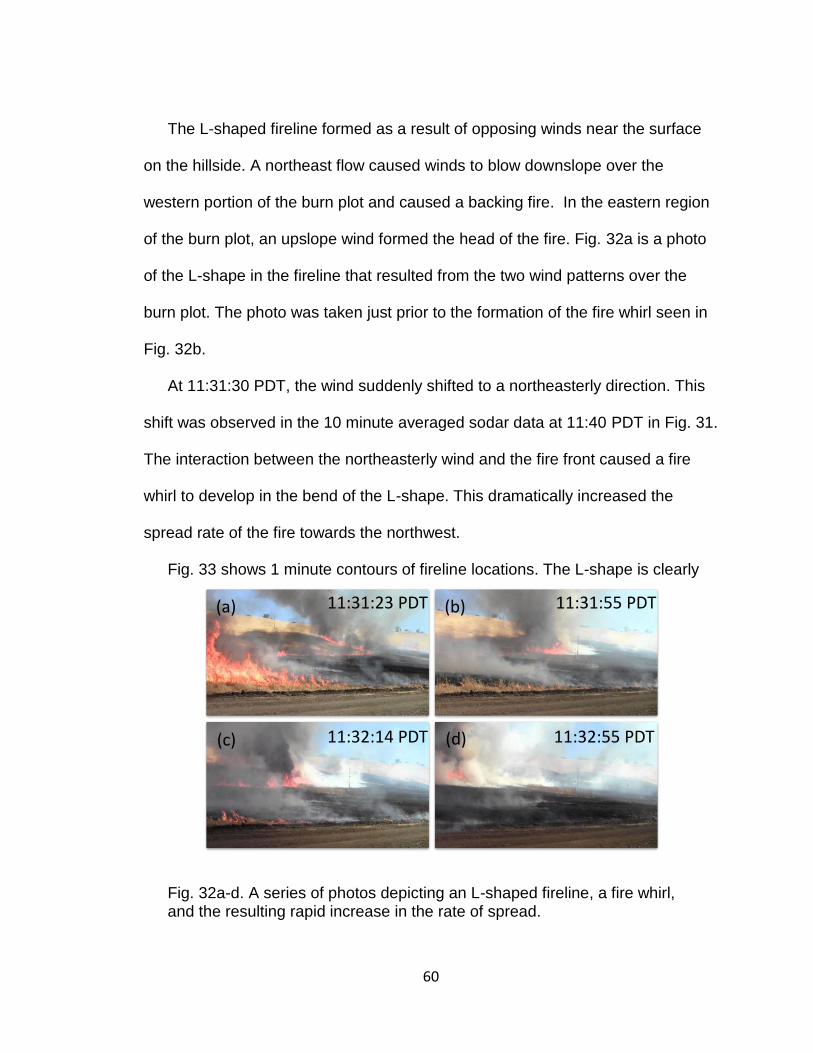
60

The L-shaped fireline formed as a result of opposing winds near the surface

on the hillside. A northeast flow caused winds to blow downslope over the

western portion of the burn plot and caused a backing fire. In the eastern region

of the burn plot, an upslope wind formed the head of the fire. Fig. 32a is a photo

of the L-shape in the fireline that resulted from the two wind patterns over the

burn plot. The photo was taken just prior to the formation of the fire whirl seen in

Fig. 32b.

At 11:31:30 PDT, the wind suddenly shifted to a northeasterly direction. This

shift was observed in the 10 minute averaged sodar data at 11:40 PDT in Fig. 31.

The interaction between the northeasterly wind and the fire front caused a fire

whirl to develop in the bend of the L-shape. This dramatically increased the

spread rate of the fire towards the northwest.

Fig. 33 shows 1 minute contours of fireline locations. The L-shape is clearly

11:32:55 PDT 11:32:14 PDT

11:31:55 PDT 11:31:23 PDT

Fig. 32a-d. A series of photos depicting an L-shaped fireline, a fire whirl, and the resulting rapid increase in the rate of spread.

(d)

(b) (a)

(c)

61

defined in the 14 minute contour. This was followed by a large gap between the

contours indicating the increased spread of the fire.

A diagnosis of this event was made difficult because of sparse data points.

But two hypotheses were developed from the data available based on horizontal

and vertical vorticity.

5.4 Results

5.4.1 Horizontal Vorticity

Between 11:30 and 11:40 PDT, sodar data indicated the development of a

strong northeasterly wind. As this northeasterly wind aloft moved over the

southerly wind within the valley, shear vorticity was generated over the fireline. A

lidar RHI scan from this time (Fig. 34) shows the inbound northeasterly wind

Fig. 33. A map of 1 minute interval fireline locations georeferenced from aerial photography. Figure produced by Dianne Hall and used with permission.

62

above the outbound southeasterly surface wind. This event corresponded well

with the observed timing of the fire whirl and rapid intensification of the fire

spread captured in Figs. 32a-d.

Fig. 35 shows a time series of the estimated horizontal vorticity from the

bottom two towers during the time frame of the event. The maximum estimated

horizontal vorticity of -0.2 s-1 occurred at approximately 11:31:35 PDT. The

heated buoyant air tilted the vorticity vertically over the fireline and the rotation

intensified as the whirl was stretched within the bend of the L-shaped fire front.

Fig. 34 Lidar RHI scan taken during the northeasterly wind. Outbound winds in warmer colors near the surface show the valley winds. The cooler colors aloft represent the northeasterly wind.

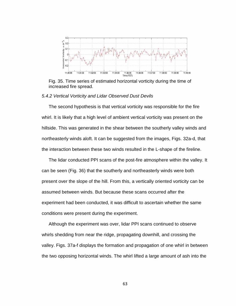
63

5.4.2 Vertical Vorticity and Lidar Observed Dust Devils

The second hypothesis is that vertical vorticity was responsible for the fire

whirl. It is likely that a high level of ambient vertical vorticity was present on the

hillside. This was generated in the shear between the southerly valley winds and

northeasterly winds aloft. It can be suggested from the images, Figs. 32a-d, that

the interaction between these two winds resulted in the L-shape of the fireline.

The lidar conducted PPI scans of the post-fire atmosphere within the valley. It

can be seen (Fig. 36) that the southerly and northeasterly winds were both

present over the slope of the hill. From this, a vertically oriented vorticity can be

assumed between winds. But because these scans occurred after the

experiment had been conducted, it was difficult to ascertain whether the same

conditions were present during the experiment.

Although the experiment was over, lidar PPI scans continued to observe

whirls shedding from near the ridge, propagating downhill, and crossing the

valley. Figs. 37a-f displays the formation and propagation of one whirl in between

the two opposing horizontal winds. The whirl lifted a large amount of ash into the

Fig. 35. Time series of estimated horizontal vorticity during the time of increased fire spread.

64

air, allowing elevated levels of backscatter to be measured in the vicinity of the

whirl. Several photos were also captured of the whirls (Fig. 38).

5.4.3 Discussion

Some numerical modeling has been performed in the area of lee side fire

spread on a slope. Simpson et al. (2013) used the WRF-Fire model to perform

2D and 3D simulations of lee side fire spread in varying atmospheric stabilities. It

was found that strong positive vorticity is typically generated near the top of the

leeward slope and extended roughly 1 km downwind of the ridge. Additionally,

Fig. 36. A lidar PPI scan of alternating inbound and outbound winds over the valley. Cooler colors represent inbound winds; warmer colors are outbound winds. The laser collided with the hillside at ~1km, resulting in the elevated backscatter and a high level of noise in the leeward section.

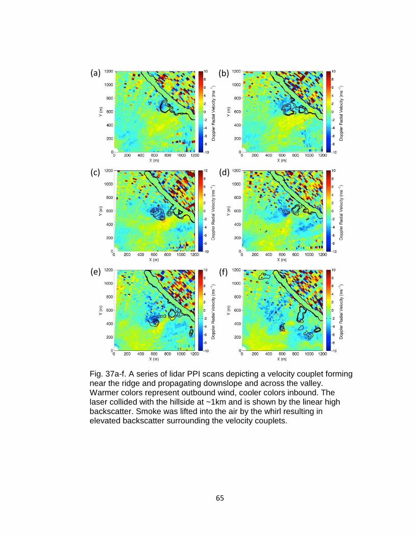
65

Fig. 37a-f. A series of lidar PPI scans depicting a velocity couplet forming near the ridge and propagating downslope and across the valley. Warmer colors represent outbound wind, cooler colors inbound. The laser collided with the hillside at ~1km and is shown by the linear high backscatter. Smoke was lifted into the air by the whirl resulting in elevated backscatter surrounding the velocity couplets.

(a) (b)

(c) (d)

(f) (e)

66

it was shown that leeside winds were dominated by small-scale turbulence rather

than a leeside rotor. A high degree of spatial variability was also found in the

average horizontal winds for the 3D model runs, which agrees well with the

Doppler lidar PPI scans. These model simulations fit well with the vertical vorticity

hypothesis. The propagating vorticity, generated near the ridge between the

Fig. 38. A photo of a whirl lifting ash into the air in the wake of the fire.

67

southerly wind within the valley and the northeasterly wind above, was tilted

vertically over the fire.

Simpson et al. went on to discuss the vertical velocity over the slope after the

fire. He showed that areas of updraft and downdraft occurred on opposing sides

of the fireline. This caused an area of counterclockwise rotating flow. This fits

exceptionally well with the “L-shaped” fireline and what was observed. They also

found that the updraft-downdraft interfaced led to a doubling of the lateral fire

spread, which agrees exceptionally well with our observations.

In a separate paper, Simpson et al. (2014) explored vorticity driven lateral fire

spread using the WRF-fire model. They identified three distinct stages of spread.

First, fire spreads upslope towards the ridge. Second, the fire spreads laterally at

a higher rate than the base spread. Third, lateral spread becomes intermittent

and at a high rate near the ridge. Using a fire-atmosphere coupled WRF-FIRE

model, Simpson et al. linked fire whirls occurring near the fireline to rapid lateral

fire spread on a slope. The simulations were repeated with a non-coupled fire-

atmosphere. It was shown that fire whirls did not occur near the fireline and the

fire spread very little laterally as a result. This indicated that vorticity generated

fire whirls were the result of interactions between the fire, atmosphere, and

terrain.

The observations from our experiment support the coupled models results. An

elevated level of vorticity was observed during the development of the fire whirl

within the L-shape bend in an asymmetrical fireline. This caused a rapid increase

68

in the lateral fire spread on the slope as seen in the photos and map of fireline

contours.

5.5 Summary and Conclusion

During an experiment in complex terrain, a unique event occurred in which a

fire whirl caused a sudden and rapid increase in fire spread. Based on previous

literature, it was postulated that the cause of this event was related to fireline

geometry and either horizontal or vertical vorticity. The opposing southeasterly

and northeasterly winds made determining the axis of the vorticity difficult. A

strengthening northeasterly wind was observed by Doppler lidar just prior to the

event causing strong horizontal vorticity to develop. The lidar also observed the

two winds on a horizontal plane during a period after the fire. It was suggested

that areas of vertical vorticity could be present above the burn area between the

two winds. As a result, fire whirls were a common occurrence at this time.

Chapter 6 - Summary and Conclusion

An experiment was conducted on a hillside in which a prescribed head fire

was ignited. The purpose was to collect data and observe the atmosphere

surrounding a fire on a hillside under ideal conditions. The data set could then be

used to compare numerical simulations.

An array of meteorological instrumentation was deployed within a valley in

central California. Sensors measuring temperature, pressure, three-dimensional

winds, and radiation were attached to three towers that spanned the burn plot.

Among them were thermocouples, barometers, sonic anemometers, and

69

radiometers. Remote sensing measurements were made using a Doppler lidar, a

microwave profiler, and a Doppler sodar.

Data from the experiments were presented in three chapters. Among the data

presented were pressure-temperature perturbations, micrometeorology, and

vorticity observations. Negative covariances were observed between pressure

and temperature. It was found that the magnitude of each covariance was

determined by the intensity of the fire. The negative values were primarily caused

by negative pressure tendencies resulting from surface convergence into the

plume. The increased amplitude of the covariances was a result of the extreme

temperature perturbations. Due to an underdeveloped fire front at the time of

FFP, several of the covariances were substantially weaker. Further

experimentation should be conducted on a more idealized fire to determine the

utility of pressure-temperature covariances for fire behavior analysis.

Observations of TKE and sensible heat flux were made as the fire propagated

upslope. Measurements at the bottom tower showed the highest values. This

FFP occurred during a time period in which the fire was mostly a head fire. The

FFP at the second tower showed a much lower value of TKE. Here the fire had

become a backing fire. Downslope winds at this time resulted in a negative heat

flux. At the top tower, the low intensity backing fire continued. The stronger

northerly winds near the ridge top pushed the plume through the sonic

anemometer several times, resulting in sporadic increases of TKE.

70

The turbulence spectra during FFP at each tower were also compared. The

most significant observation was the elevated values in the mid to high

frequencies of vertical velocity at the bottom tower. This was the result of the

elevated fire intensity during FFP at the bottom tower. The middle and top towers

did not observe an increase in vertical velocity spectra. This was caused by a

transition in fire behavior from a heading fire to a backing fire, resulting in much

lower intensity during the two FFPs.

A case can be made for the presence of both horizontal and vertical vorticity

presence on the slope during the experiment. It was determined from previous

numerical modeling studies that horizontal vorticity was most likely the driver of

the rapid lateral spread. RHI scans performed by the Doppler lidar revealed an

area of strong shear where horizontal vorticity could occur. Estimates from the

sonic anemometers showed increased horizontal vorticity during a fire whirl and

subsequent rapid fire spread.

Vertical vorticity was supported by PPI scans from the lidar taken during the

post experiment. Areas of outbound and inbound winds were observed on a

horizontal plane over the slope. Additionally, rotational couplets were observed

occurring between these areas of opposing winds. Dust devils were

photographed occurring at these times and could be a catalyst for the fire whirl

that occurred.

71

REFERENCES

Albini, F. A., R. G. Baughman, 1979: Estimating windspeeds for predicting wildland fire behavior. USDA Forest Service Research Paper INT (USA), .

Andrews, P. L., 1986: BEHAVE: fire behavior prediction and fuel modeling system-BURN subsystem, Part 1.

Beals, E. A., 1914: value of weather forecasts in the problem of protecting forests from fire.

Bowman, D. M., J. K. Balch, P. Artaxo, W. J. Bond, J. M. Carlson, M. A. Cochrane, C. M. D'Antonio, R. S. Defries, J. C. Doyle, S. P. Harrison, F. H. Johnston, J. E. Keeley, M. A. Krawchuk, C. A. Kull, J. B. Marston, M. A. Moritz, I. C. Prentice, C. I. Roos, A. C. Scott, T. W. Swetnam, G. R. van der Werf, and S. J. Pyne, 2009: Fire in the Earth system. Science, 324, 481-484, doi:10.1126/science.1163886 [doi].

Clements, C. B., 2010: Thermodynamic structure of a grass fire plume. Int.J.Wildland Fire, 19, 895-902.

Clements, C. B., R. Perna, M. Jang, D. Lee, M. Patel, S. Street, S. Zhong, S. Goodrick, J. Li, and B. E. Potter, 2007: Observing the dynamics of wildland grass fires: FireFlux-a field validation experiment. Bull.Am.Meteorol.Soc., 88, 1369-1382.

Clements, C. B., S. Zhong, X. Bian, W. E. Heilman, and D. W. Byun, 2008: First observations of turbulence generated by grass fires. Journal of Geophysical Research: Atmospheres (1984–2012), 113.

Clements, C. B. and A. J. Oliphant, 2014: The California State University Mobile Atmospheric Profiling System: A Facility for Research and Education in Boundary Layer Meteorology. Bull. Amer. Meteor. Soc., 95, 1713–1724.

Cunningham, P., R. R. Linn, 2007: Numerical simulations of grass fires using a coupled atmosphere‐fire model: Dynamics of fire spread. Journal of Geophysical Research: Atmospheres (1984–2012), 112.

Dennison, P. E., K. Charoensiri, D. A. Roberts, S. H. Peterson, and R. O. Green, 2006: Wildfire temperature and land cover modeling using hyperspectral data. Remote Sens.Environ., 100, 212-222.

72

Filippi, J., X. Pialat, and C. B. Clements, 2013: Assessment of ForeFire/Meso-NH for wildland fire/atmosphere coupled simulation of the FireFlux experiment. Proceedings of the Combustion Institute, 34, 2633-2640.

Finney, M. A., 1998: FARSITE users guide and technical documentation. USDA Forest Service Research Paper RMRS-RP-4, .

Huang, C., Y. Lin, M. Kaplan, and J. Charney, 2009: Synoptic-scale and mesoscale environments conducive to forest fires during the October 2003 extreme fire event in southern California. Journal of Applied Meteorology and Climatology, 48, 553-579.

Kitzberger, T., P. M. Brown, E. K. Heyerdahl, T. W. Swetnam, and T. T. Veblen, 2007: Contingent Pacific-Atlantic Ocean influence on multicentury wildfire synchrony over western North America. Proc.Natl.Acad.Sci.U.S.A., 104, 543- 548, doi:0606078104 [pii].

Kochanski, A. K., M. A. Jenkins, J. Mandel, J. Beezley, and S. Krueger, 2013: Real time simulation of 2007 Santa Ana fires. For.Ecol.Manage., 294, 136- 149.

Linn, R. R., J. L. Winterkamp, D. R. Weise, and C. Edminster, 2010: A numerical study of slope and fuel structure effects on coupled wildfire behaviour. Int.J.Wildland Fire, 19, 179-201.

Linn, R., J. Winterkamp, C. Edminster, J. J. Colman, and W. S. Smith, 2007: Coupled influences of topography and wind on wildland fire behaviour. Int.J.Wildland Fire, 16, 183-195.

Mell, W. E., K. B. McGrattan, and H. R. Baum, 1996: Numerical simulation of combustion in fire plumes. Proc. Symposium (International) on Combustion, Elsevier, 1523-1530.

Rehm, R. G., H. R. Baum, 1978: The Equations of Motion for Thermally Driven, Buoyant Flows. Journal of Research of the National Bureau of Standards, 83, 297-308.

Rothermel, R. C., 1972: A mathematical model for predicting fire spread in wildland fuels.

Rothermel, R. C., 1983: How to predict the spread and intensity of forest and range fires.

73

Šavli, M., 2012: Turbulence kinetic energy–TKE. Proc. University of Ljubljana, Faculty of Mathematics and Physics, Department of Meteorology. Seminar: 4th Class. May, .

Schroeder, M. J., M. Glovinsky, V. F. Henricks, F. C. Hood, and M. K. Hull, 1964: Synoptic weather types associated with critical fire weather, .

Simpson, C. C., J. J. Sharples, J. P. Evans, and M. F. McCabe, 2013: Large eddy simulation of atypical wildland fire spread on leeward slopes. Int.J.Wildland Fire, 22, 599-614.

Simpson, C. C., J.J. Sharples, and J.P. Evans, 2014: Resolving vorticity-driven lateral fire spread using the WRF-Fire coupled atmosphere–fire numerical model, Nat. Hazards Earth Syst. Sci., 14, 2359-2371.

Viegas, D. X., 2004: Slope and wind effects on fire propagation. Int.J.Wildland Fire, 13, 143-156.

Walker, J., B. Stocks, 1968: Thermocouple errors in forest fire research. Fire Technol., 4, 59-62.

Westerling, A. L., H. G. Hidalgo, D. R. Cayan, and T. W. Swetnam, 2006: Warming and earlier spring increase western U.S. forest wildfire activity. Science, 313, 940-943, doi:1128834 [pii].